Embed Size (px)
Citation preview
Available online at www.sciencedirect.com
Computers & Operations Research 31 (2004) 157–180www.elsevier.com/locate/dsw
A new heuristic for m-machine &owshop scheduling problemwith bicriteria of makespan and maximum tardiness
Ali Allahverdi∗
Department of Industrial and Management Systems Engineering, College of Engineering and Petroleum,Kuwait University, P.O. Box 5969, Safat 13060, Kuwait
Received 1 July 2001; received in revised form 1 March 2002
Abstract
This paper addresses the m-machine &owshop problem with the objective of minimizing a weighted sum ofmakespan and maximum tardiness. Two types of the problem are addressed. The 2rst type is to minimize theobjective function subject to the constraint that the maximum tardiness should be less than a given value. Thesecond type is to minimize the objective without the constraint. A new heuristic is proposed and compared totwo existing heuristics. Computational experiments indicate that the proposed heuristic is much better than theexisting ones. Moreover, a dominance relation and a lower bound are developed for a three-machine problem.The dominance relation is shown to be quite e5cient.
Scope and purpose
The majority of research on scheduling problems addresses only a single criterion while the majority ofreal-life problems require the decision maker to consider more than a single criterion before arriving ata decision. The scheduling literature reveals that the research on multi-criteria is mainly focused on thesingle-machine problem as a result of the di5culty of the multiple machines problem. This paper addressesan m-machine &owshop scheduling problem with a multi-criteria objective function.? 2003 Elsevier Ltd. All rights reserved.
Keywords: Flowshop; Bicriteria; Makespan; Tardiness; Heuristic; Dominance relation
1. Introduction
Makespan and maximum tardiness are among the most commonly used criteria in the &owshopscheduling research. Makespan is a measure of system utilization while maximum tardiness is a
∗ Tel.: +965-484-1188; fax: +965-481-6137.E-mail address: [email protected] (A. Allahverdi).
0305-0548/04/$ - see front matter ? 2003 Elsevier Ltd. All rights reserved.PII: S0305-0548(02)00143-0
158 A. Allahverdi / Computers & Operations Research 31 (2004) 157–180
measure of performance in meeting customer due dates. The makespan criterion for m-machine&owshop has been addressed in the literature by many researchers including Nawaz et al. [1], Chuet al. [2], Zegordi et al. [3], and Riane et al. [4]. The tardiness criterion has also been addressed inthe literature by many researchers, e.g., Townsend [5], Kim [6,7], Srinivasaraghavan and Rajendran[8], and Armentano and Ronconi [9].
The research mentioned so far addressed only a single criterion while the majority of real lifeproblems require the decision maker to consider more than a single criterion before arriving at adecision. The research on multiple criteria is mainly focused on the single machine scheduling prob-lem, see Nagar et al. [10]. The reason for this is that the scheduling problem with multiple-machineis di5cult even with a single criterion. Therefore, considering more than a single criterion makesthe multiple-machine problem even more di5cult to solve.
This paper considers both makespan and maximum tardiness as the performance measures wherethe objective is to minimize a weighted sum of makespan and maximum tardiness. A survey of theliterature has revealed that the m-machine problem with this objective function is addressed onlyby Daniels and Chambers [11] and Chakravarthy and Rajendran [12]. Both papers addressed theproblem in order to minimize the objective function value subject to the constraint that maximumtardiness is not greater than a given value. Daniels and Chambers [11] provided two dominancerelations and developed a lower bound for the two-machine problem, and presented two heuristicalgorithms; one for the two-machine and the other for the m-machine problem. Chakravarthy andRajendran [12] presented a simulated annealing algorithm for the m-machine problem and comparedtheir algorithm with that of Daniels and Chambers [11].
This paper considers the same problem addressed by Daniels and Chambers [11] and Chakravarthyand Rajendran [12]. The paper also considers the problem without the constraint on the maximumtardiness. A new heuristic is proposed and shown by extensive computational experiments that theproposed heuristic perform much better than those of Daniels and Chambers [11] and Chakravarthyand Rajendran [12]. Furthermore, an e5cient dominance relation and a lower bound are establishedfor the three-machine problem.
2. Problem formulation
Let n be the number of jobs, m the number of machines, Cmax the makespan, Tmax the maximumtardiness, ti; j the processing time of job i on machine j, t[i; j] the processing time of the job inposition i on machine j; di the due date of job i; d[i] the due date of the job in position i; T[i] thetardiness of the job in position i and C[i; j] the completion time of the job in position i on machine j.Then, Cmax = C[n;m] and Tmax = max{max(C[i;m] − d[i]; 0) for i = 1; 2; : : : ; n}.The objective function value (OFV) is de2ned by �Cmax+(1−�)Tmax where 06 �6 1. � denotes
the weight (or relative importance) given to Cmax and Tmax. Given this objective function, two typesof the problem can be de2ned:
Problem 1 (P1).Minimize �Cmax + (1− �)Tmax
Subject to Tmax6K;
where K is a value speci2ed by the scheduler.
A. Allahverdi / Computers & Operations Research 31 (2004) 157–180 159
Problem 2 (P2).
Minimize �Cmax + (1− �)Tmax:
In this paper both problems P1 and P2 are addressed. Notice that Daniels and Chambers [11]and Chakravarthy and Rajendran [12] only considered P1. In this paper, as well as in the papersby Daniels and Chambers [11] and Chakravarthy and Rajendran [12], permutation schedules areconsidered.
3. A dominance relation and a lower bound
Dominance relations are known to improve the e5ciency of implicit enumeration techniques suchas branch-and-bound or dynamic programming. Daniels and Chambers [11] established two domi-nance relations and a lower bound for a two-machine &owshop. In this section, a dominance relationand a lower bound are developed for a three-machine &owshop. The e5ciency of the dominancerelation is shown in Section 5.
Let TPj; k represent the total processing time of the jobs in positions 1; 2; : : : ; j on machine k,i.e., TPj; k = t[1; k] + · · · + t[j; k]. Also let �j;k be the total idle time on the kth machine up to thecompletion time of the job in position j. Let �j;2 =TPj;1−TPj−1;2 where TP0;2 =0. It is known that�j;2 =max{�1;2; �2;2; : : : ; �j;2}. If �j;3 =�j;2 + TPj;2 − TPj−1;3 where P0;3 = 0, it can be shown that�j;3 = max{�1;3; �2;3; : : : ; �j;3}. Thus, Cj;3 = TPj;3 +�j;3. From the above de2nitions, the makespanfor a three-machine &owshop is given by Cmax = TPn;3 + �n;3. Since the value of the term TPn;3 isconstant regardless of the sequence, minimizing Cmax is equivalent to minimizing �n;3.
Let Li denote the lateness of the job in position i, i.e., Li =C[i;3] − d[i] and let Lmax represent themaximum lateness.
Consider exchanging the positions of two adjacent jobs on a three-machine &owshop in an optimalsequence �1 that has job i in position � and job j in position �+1. Call the sequence obtained from�1 as �2, i.e., �1 = : : : ; i; j; : : : and �2 = : : : ; j; i; : : : :
Lemma 1. For both sequences �1 and �2; �r;2(�1)=�r;2(�2) for r=1; 2; : : : ; �−1; �+2; �+3; : : : ; n.
Proof. Since both sequences have the same jobs in positions 1; 2; : : : ; � − 1; �r;2(�1) = �r;2(�2) forr=1; 2; : : : ; �−1. Furthermore, �r;2(�1)=�r;2(�2) for r=�+2; �+3; : : : ; n since again both sequenceshave the same jobs in these positions, and both include the jobs in positions � and �+ 1.
Lemma 2. �r;3(�1)=�r;3(�2) for r=1; 2; : : : ; �−1, and �r;3(�2)6�r;3(�1) for r= �+2; �+3; : : : ; nif max{��;2(�2); ��+1;2(�2)}6max{��;2(�1); ��+1;2(�1)}.
Proof. It is clear that �r;3(�1) = �r;3(�2) for r = 1; 2; : : : ; �− 1 since both sequences have the samejobs in these positions. Now, it follows by de2nition of �r;3 that for r = �+ 2; �+ 3; : : : ; n
�r;3(�2)− �r;3(�1) =max{�1;2(�2); : : : ; ��;2(�2); ��+1;2(�2); : : : ; �r;2(�2)}−max{�1;2(�1); : : : ; ��;2(�1); ��+1;2(�1); : : : ; �r;2(�1)}:
If max{��;2(�2); ��+1;2(�2)}6max{��;2(�1); ��+1;2(�1)}, then by Lemma 1, �r;3(�2)6�r;3(�1).
160 A. Allahverdi / Computers & Operations Research 31 (2004) 157–180
Lemma 3. Lr(�2) = Lr(�1) for r = 1; 2; : : : ; � − 1. Moreover, if max{��;3(�2); ��+1;3(�2)}6max{��;3(�1); ��+1;3(�1)} and max{��;2(�2); ��+1;2(�2)}6max{��;2(�1); ��+1;2(�1)}, then Lr(�2)6Lr(�1) for r = �+ 2; �+ 3; : : : ; n.
Proof. Since both sequences have the same job in positions 1; 2; : : : ; � − 1; Lr(�2) = Lr(�1) forr = 1; 2; : : : ; �− 1. For r = �+ 2; �+ 3; : : : ; n, taking the diMerence between Lr(�2) and Lr(�1) yields
Lr(�2)− Lr(�1) =max{�1;3(�2); : : : ; ��;3(�2); ��+1;3(�2); : : : ; �r;3(�2)}−max{�1;3(�1); : : : ; ��;3(�1); ��+1;3(�1); : : : ; �r;3(�1)}:
If max{��;2(�2); ��+1;2(�2)}6max{��;2(�1); ��+1;2(�1)} and max{��;3(�2); ��+1;3(�2)}6max{��;3(�1); ��+1;3(�1)} then by Lemmas 1 and 2, Lr(�2)6Lr(�1).
Theorem. Consider a three-machine 9owshop and suppose that two adjacent jobs i and j satisfy
(i) dj6di and either(iia) tj;26 ti;2 and tj;16 ti;1 or(iib) ti;36 ti;2 and either tj;16 ti;1 or ti;26 ti;1 and either(iiia) ti;26 tj;3 and ti;16 tj;2 or(iiib) tj;26 tj;3 and either ti;16 tj;2 or tj;16 tj;2 or(iiic) ti;36 tj;3 and either ti;16 tj;2 or tj;16 tj;2.
Then, there exists an optimal solution with respect to minimizing both Cmax and Lmax in which jobj precedes job i.
Proof. See Appendix A.Note that in the Theorem, the values of Cmax and Lmax are minimized simultaneously if job j
precedes job i. Therefore, the function �Cmax + (1− �)Lmax is also minimized for any �. Moreover,this also minimizes our objective function of �Cmax+(1−�)Tmax for any � value since it is a knownfact that a sequence that minimizes Lmax also minimizes Tmax.The dominance relation given in the above theorem can be used either in an implicit enumeration
technique or in a heuristic. The developed relation is used in the proposed heuristic (next section)for the case of three-machine problem. Dominance relations are very useful particularly when used inimplicit enumeration techniques. In order to check the developed relation’s e5ciency, a lower boundis established in Appendix B and it is used in a Branch-and-Bound algorithm, which is applied inthe regular way by using the depth-2rst strategy. The e5ciencies of the dominance relation and thebranch-and-bound (the lower bound) algorithm are brie&y investigated in Section 5.
4. Heuristics
A survey of literature has revealed that the problem considered in this paper has been addressedby Daniels and Chambers [11] and Chakravarthy and Rajendran [12], each providing a heuristicalgorithm. In this section, their heuristics are brie&y de2ned and a new heuristic is proposed.
A. Allahverdi / Computers & Operations Research 31 (2004) 157–180 161
4.1. Existing heuristics
4.1.1. Daniels and chambers heuristic (DCH)The 2rst heuristic for our problem was established by Daniels and Chambers [11]. For each
position, a set of eligible jobs is determined and one of these eligible jobs is chosen based on itsposition in Nawaz et al. [1] sequence, also known as NEH. The NEH sequence is used since it isknown that this sequence performs well for minimizing Cmax. For a given K value as an upper boundfor Tmax, the DCH determines a subset of jobs that may occupy the last position of the sequence.Job i is eligible for the last position if
∑nj=1 tj;1 +
∑mr=2 ti; r − di6K . The job with the largest
completion time in NEH sequence, among the ones that are eligible to occupy the last position, ischosen for the last position of DCH sequence. Then, the eligible jobs among the remaining n−1 jobsfor the second last position of DCH sequence are determined. The job for the second last positionof DCH is chosen to be the one, among those eligible ones, with the largest completion time inNEH sequence. This process continues until all the positions of DCH are occupied, i.e., until all thejobs are assigned. In the case this sequence violates the upper limit of K , the procedure backtracksto the last job in the sequence with excess tardiness and replaces it with a diMerent eligible job forthe corresponding position. The criterion for selecting a diMerent job for the corresponding positionis to choose the untested eligible job with the largest completion time in the NEH sequence. If thisalso violates the upper limit K , then this process is repeated until a feasible sequence in obtained.This feasible value of maximum tardiness is then decremented to get the tardiness constraint for thenext iteration of the procedure. The process is repeated until no feasible sequence can be generated.
4.1.2. Simulated annealing heuristic (SAH)Chakravarthy and Rajendran [12] were the second to address our problem and they developed
another heuristic by using the simulated annealing technique. They use three methods to generatethree sequences and choose the best one as an initial sequence. This sequence is given as an inputto the simulated annealing algorithm.
These three methods are the earliest due date (EDD), least static slack (LSS), and the heuris-tic by Nawaz et al. [1] (NEH). The EDD and LSS sequences seek to minimize Tmax while theNEH sequence seeks to minimize Cmax. The EDD sequence is obtained from ordering the jobs bynon-decreasing order of their due dates. The slack value of a job is obtained by subtracting the sumof the processing times of all operations of the job on each machine from the job’s due date. Then,the LSS sequence is obtained by ordering the jobs in non-decreasing order of their slack values.
They have obtained the appropriate parameters for the algorithm after some pilot runs. Based onthese pilot runs, they have chosen an initial temperature of 475 and the temperature reduction factorof 0.9, and hence, allowing the algorithm to run for 30 temperature stages. A terminating conditionis needed for each temperature. Therefore, a counter to keep track of the number of accepted movesand a counter to keep track of the total number of moves at a particular temperature are needed. Theminimum number of accepted moves needed for the termination of iterations at a given temperatureis selected to be n with an upper limit of 4n. The counter used for ending is chosen to be 5.
They have used the adjacent interchange scheme in searching for the neighborhood. A job isselected at random from the current solution. Then, a random number, uniform between 0 and 1, isgenerated. If the random number is less than or equal to 0.5, the chosen job in the current sequence
162 A. Allahverdi / Computers & Operations Research 31 (2004) 157–180
is interchanged with the adjacent job to its left, otherwise with the adjacent job to its right. If thesequence obtained after the interchange does not satisfy the condition on the Tmax, the process ofrandomly choosing a job and interchanging it with the one to its left or right continues until thenew sequence satis2es the condition.
SAH was run with the parameters speci2ed above. It has been found that it consumes less timethan the proposed heuristics. Therefore, in order to have a fair comparison, the reduction factor hasbeen changed to 0.995 which gives more computational time to SAH. This has improved the errorperformance of SAH and made it possible to have a fair comparison.
4.1.3. Modi>ed NEH (MNEH)The NEH was originally developed for the objective of makespan. It can be modi2ed for the
objective considered in this paper, which is called modi2ed NEH or MNEH in this paper. Solutionsobtained from MNEH are compared with the 2nal solutions of the existing heuristics of DCH andSAH, and with that of the proposed heuristic explained next.
4.2. Proposed heuristic (PH)
An input parameter, called L, is needed for the proposed heuristic. This parameter denotes thenumber of times certain steps of the heuristic (steps 5–7) are repeated. Two values of 5 and 10 arechosen for L based on some pilot runs. PH(L = 5) and PH(L = 10) denote the proposed heuristicwith these L values.
Step 1: Find the EDD sequence (�1).Step 2: Find the LSS sequence (�2).Step 3: Find the MNEH sequence (�3).(if m=2, then obtain the sequence �3 by the Johnson’s algorithm since it is known to be optimal
with respect to Cmax).Step 4: Find min{OFV(�1);OFV(�2);OFV(�3)} and let the sequence yielding the minimum OFV
be called �. Let �1 = �; y = 0; h= 1, and r = 1.Step 5: Set p=1. Pick the 2rst 2 jobs from �r and schedule them in order to minimize the OFV
as if there were only 2 jobs. Select the best sequence as a current solution.Step 6: Set p=p+ 1. Generate candidate sequences by selecting the next two jobs from �r and
inserting this pth block of two jobs into each slot of the current solution, and interchanging theorder of the two jobs within the block. Among these candidates, select the best one with the leastpartial OFV. Set the best one as a current solution.Step 7: Repeat Step 6 until all the jobs in �r are assigned. Note that if the last assignment is a
single job, then treat that job as a block. Call the resulting sequence as �r+1.Step 8: If OFV(�r+1)¡OFV(�), then let �= �r+1.Step 9: Set r = r + 1. If r6L, go to Step 5.Step 10: If Tmax(�)6K , go to Step 16.Step 11: If y¿ 100n, go to Step 15.Step 12: Find job j such that Tj = Tmax(�) (i.e., Tj ¿K), assume job j is in position i. If i = 1
go to Step 15. Otherwise set g= i − 1 and y = y + 1.
A. Allahverdi / Computers & Operations Research 31 (2004) 157–180 163
Step 13: Switch the jobs in positions i and g of the sequence � if dj ¡d[g] and go to Step 10.Otherwise go to Step 14.Step 14: g= g− 1. Go to Step 13 if g �= 0.Step 15: Set K = Tmax(�).Step 16: Switch the jobs in position h and h+1 of the sequence � if Tmax(after switch) 6K and
OFV of the sequence after the switch is less than that of �, then update � by switching the twojobs.Step 17: Let h= h+ 1, go to Step 16 if h¡n.Step 18: The last updated sequence � is the heuristic sequence.
If the problem is three-machine problem, then in Step 16 of the algorithm, there is no need toswitch the jobs in position h and h+1 if the jobs in these two positions satisfy the conditions statedin the Theorem.
The PH heuristic can be summarized as follows:
Step 1: Set the parameters L and K .Step 2: Get an initial solution.Step 3: Apply the proposed insertion technique L times.Step 4: Repair if K is violated (for Problem 1).Step 5: Apply the proposed local search technique.
4.3. K value
Daniels and Chambers [11] de2ned the value of K to be Tmax of the NEH sequence meaning thatthere is at least one sequence that is feasible with respect to this K value. Then, the feasible value ofK is incrementally reduced, yielding a new K value for the next iteration. The process is continueduntil no feasible schedule can be generated. Therefore, there exists no situation where the conditionTmax6K cannot be satis2ed. This feasibility condition is satis2ed by the backtracking process ofDCH.
Chakravarthy and Rajendran [12] de2ned a K value to be
K = !maxr
maxi
m∑j=1
ti; j + (n− 1)
/n
n∑g=1
tg;m
− dr
;
where != 1. This K value also ensures the feasibility condition. They use the adjacent interchangescheme for the neighborhood search in the Simulated Annealing algorithm. If the neighborhoodsequence does not satisfy the feasibility, then the adjacent interchange scheme is repeated until afeasible sequence is obtained.
If this K value with !=1 is used, then Steps 11 and 15 of the proposed heuristic can be deletedsince the feasibility is guaranteed. Steps 12–14 of the algorithm ensure the feasibility.
In addition to the case when ! = 1, in this paper, the performance of the two existing and theproposed heuristics is investigated for the cases when ! = 0:8 and 0.9. Observe that for the casewhen !¡ 1 (depending on how much it is less than one), it may not be possible to 2nd a feasibleschedule. Therefore, a limit of n× 100 is imposed for the number of searches for feasibility. This is
164 A. Allahverdi / Computers & Operations Research 31 (2004) 157–180
the maximum number for backtracking steps for DCH, the number of adjacent interchange schemesfor SAH (note this is not the number of neighborhood searches but rather the number for feasibilitysearches), and y value in the proposed heuristic. For all heuristics when this limit is reached, thesearch for feasibility is stopped and the last sequence is taken to be the solution. It should be notedthat when this limit is reached it does not necessarily mean that the problem is infeasible. Thenumber n× 100 is chosen based on computational experience. In fact, for the feasible cases, it hasbeen observed that the number of times for searching the feasibility for all heuristics is much lowerthan this number. It should be also noted that Chakravarthy and Rajendran [12] did not put anylimit since they experimented with smaller number of jobs and only considered the K value when!= 1.
5. Comparison of DCH, SAH, MNEH and PH
An extensive evaluation of the existing heuristics DCH, SAH, MNEH and the proposed heuristicwith two levels of L (PH(L=5) and PH(L=10)) is conducted. The existing and proposed heuristicswere coded in FORTRAN language and run on a SUN SPARC Station 20. The processing times oneach machine were randomly generated from a discrete uniform distribution in the range [1, 100].This is a common range used in the literature, e.g., Chakravarthy and Rajendran [12], Rajendranand Ziegler [13] and Woo and Yim [14].Three performance measures are used for comparison: average percentage error (Avg.), standard
deviation (Std.), and the number of times the best solution is obtained (NB) in 30 replicates. Theheuristic percentage error is de2ned as 100(Heuristic− Best Solution)=Best Solution.
Problem 1 (P1). The job due dates have been randomly set in the range {∑mj=1 ti; j ;
∑mj=1 ti; j +
0:5(n − 1)n∑n
g=1 tg;m}. Chakravarthy and Rajendran [12] used these due dates to compare theirheuristic with DCH. Therefore, the same job due dates are used to compare the proposed heuristicwith the SAH of Chakravarthy and Rajendran and the DCH of Daniels and Chambers.
Chakravarthy and Rajendran used the following K value for ! = 1. In addition to this K value,two other K values are used when ! = 0:8 and 0.9. Three values of 0.25, 0.5, and 0.75 are usedfor the weight given to makespan, �. Chakravarthy and Rajendran also used these three values.
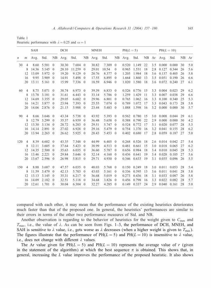
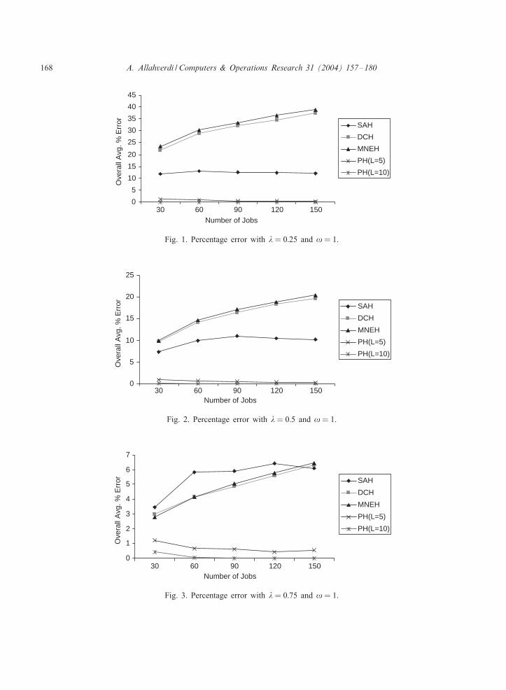
Tables 1–3 provide the performance measures of all heuristics for the K value used byChakravarthy and Rajendran (i.e., when ! = 1) for � = 0:25, 0.5, and 0.75, respectively. It canbe seen from the tables that the proposed heuristic with both levels PH(L = 5) and PH(L = 10)perform signi2cantly better than the existing heuristics DCH, SAH, MNEH in terms of all the threeperformance measures Avg., Std., and NB. Figs. 1–3 summarises average errors of all the heuristicswith respect to the number of jobs for �= 0:25, 0.5, and 0.75, respectively. For a given number ofjobs, the overall Avg. % error in the 2gures represents the average error of the 2ve average errorsfor the number of machines 4, 8, 12, 16, and 20. The superiority of the proposed heuristic over theexisting ones can also be easily seen from these 2gures. The errors for DCH and MNEH increaseby the number of jobs for all values of �. The SAH error remains unchanged for �= 0:25 and 0.5while there is a slight increase for � = 0:75 as the number of jobs increases. The errors, however,for PH(L = 5) and PH(L = 10) decrease as the number of jobs increases for all � values. This isanother advantage of the proposed heuristic over the existing ones. Notice that since heuristics are
A. Allahverdi / Computers & Operations Research 31 (2004) 157–180 165
Table 1Heuristic performance with � = 0:25 and != 1
SAH DCH MNEH PH(L= 5) PH(L= 10)
n m Avg. Std. NB Avg. Std. NB Avg. Std. NB Avg. Std. NB Ar Avg. Std. NB Ar
30 4 8.60 5.581 0 30.30 7.684 0 30.82 7.309 0 0.520 1.149 22 3.5 0.000 0.000 30 5.08 14.36 5.145 0 28.10 11.259 0 29.01 10.54 0 0.965 1.531 18 2.8 0.127 0.344 26 5.612 13.09 5.972 0 19.20 9.129 0 20.76 8.377 0 1.205 1.984 18 3.6 0.137 0.405 26 5.816 9.95 3.909 0 14.91 5.498 0 17.55 6.895 0 1.664 1.860 13 3.5 0.051 0.190 26 6.620 13.11 5.161 0 15.99 7.336 0 18.59 6.946 0 1.020 1.580 18 3.6 0.072 0.240 27 6.1
60 4 8.75 5.071 0 38.74 6.973 0 39.39 6.833 0 0.526 0.776 15 3.3 0.004 0.023 29 6.28 13.78 3.181 0 31.61 6.443 0 33.14 5.786 0 1.259 1.429 11 3.3 0.007 0.038 29 6.612 14.69 3.355 0 29.05 6.682 0 29.96 6.801 0 0.765 1.062 16 3.3 0.100 0.340 25 5.316 14.21 3.877 0 23.94 7.393 0 25.55 7.074 0 0.789 1.072 17 3.3 0.043 0.173 28 5.820 14.06 2.876 0 21.15 5.988 0 23.44 5.483 0 1.088 1.598 16 3.2 0.000 0.000 30 5.7
90 4 8.66 3.646 0 43.34 5.738 0 43.92 5.393 0 0.562 0.780 15 3.0 0.008 0.044 29 6.18 12.79 3.299 0 35.37 6.939 0 36.48 5.658 0 0.388 0.790 22 2.9 0.000 0.000 30 4.212 13.30 3.134 0 28.72 6.283 0 29.51 5.747 0 0.524 0.772 17 3.1 0.020 0.077 28 5.316 14.14 2.891 0 27.02 6.928 0 29.16 5.479 0 0.754 1.370 16 3.2 0.041 0.155 28 6.220 13.94 2.263 0 26.62 5.925 0 28.43 5.453 0 0.402 0.680 17 2.8 0.059 0.187 27 5.0
120 4 8.39 4.602 0 43.35 7.348 0 44.99 6.405 0 0.268 0.526 18 2.6 0.014 0.042 27 5.48 12.11 3.605 0 37.64 5.423 0 38.99 4.513 0 0.481 0.661 15 3.0 0.018 0.065 27 6.212 14.35 2.500 0 35.63 6.035 0 36.60 5.787 0 0.656 0.984 18 3.4 0.010 0.045 28 5.316 13.46 2.221 0 29.84 5.646 0 32.14 4.160 0 0.436 0.641 19 3.4 0.028 0.105 27 5.620 13.67 2.596 0 26.98 5.815 0 29.71 4.930 0 0.346 0.633 19 3.1 0.035 0.096 26 5.5
150 4 8.88 3.687 0 47.57 6.035 0 48.03 5.768 0 0.150 0.249 18 3.0 0.011 0.053 28 5.48 11.59 3.479 0 42.13 5.703 0 43.03 5.161 0 0.336 0.395 13 3.6 0.011 0.041 28 5.812 13.13 3.145 0 35.31 6.217 0 36.68 5.019 0 0.273 0.436 18 3.1 0.033 0.087 26 5.816 14.09 2.182 0 32.51 5.118 0 34.68 3.826 0 0.456 0.798 16 3.3 0.022 0.082 28 5.720 12.61 1.701 0 30.04 6.304 0 32.27 4.285 0 0.149 0.337 24 2.9 0.040 0.161 28 5.0
compared with each other, it may mean that the performance of the existing heuristics deterioratesmuch faster than that of the proposed one. In general, the heuristics’ performances are similar totheir errors in terms of the other two performance measures of Std. and NB.
Another observation is regarding to the behavior of heuristics for the weight given to Cmax andTmax, i.e., the value of �. As can be seen from Figs. 1–3, the performance of DCH, MNEH, andSAH is sensitive to � value, i.e., gets worse as � decreases (when a higher weight is given to Tmax).The 2gures illustrate that the performance of PH(L = 5) and PH(L = 10) is insensitive to � value,i.e., does not change with diMerent � values.
The Ar value given for PH(L = 5) and PH(L = 10) represents the average value of r (givenin the statement of the algorithm) at which the best sequence � is obtained. This shows that, ingeneral, increasing the L value improves the performance of the proposed heuristic. It also shows
166 A. Allahverdi / Computers & Operations Research 31 (2004) 157–180
Table 2Heuristic performance with � = 0:5 and != 1
SAH DCH MNEH PH(L= 5) PH(L= 10)
n m Avg. Std. NB Avg. Std. NB Avg. Std. NB Avg. Std. NB Ar Avg. Std. NB Ar
30 4 7.96 2.937 0 15.50 5.412 0 15.83 5.420 0 0.504 0.939 19 3.1 0.025 0.130 28 5.78 8.17 2.583 0 10.36 3.557 0 10.46 4.002 0 0.939 1.386 16 3.7 0.046 0.202 28 6.412 7.69 3.577 1 9.24 4.983 1 9.41 5.040 1 0.880 1.178 16 3.6 0.034 0.093 26 6.216 6.50 4.471 3 7.21 4.653 2 7.72 5.015 3 1.184 1.618 15 3.4 0.246 0.651 25 6.420 6.33 4.599 3 5.84 3.827 3 6.38 3.847 2 1.259 1.692 14 3.4 0.271 0.841 23 6.5
60 4 7.77 3.728 0 20.64 5.375 0 21.26 5.227 0 0.413 0.816 14 3.4 0.024 0.125 28 6.08 10.84 3.297 0 17.58 4.532 0 17.74 4.637 0 0.413 0.713 16 3.5 0.031 0.119 27 6.012 11.03 2.354 0 11.53 2.930 0 12.13 3.087 0 0.795 0.969 11 3.6 0.043 0.131 26 6.716 10.37 2.615 0 11.25 3.536 0 11.97 3.546 0 0.776 1.003 15 2.7 0.077 0.207 25 6.420 9.93 2.865 0 9.63 3.867 0 10.32 3.678 0 0.579 0.862 18 3.8 0.033 0.124 27 6.0
90 4 8.62 3.655 0 24.32 4.295 0 24.81 3.579 0 0.280 0.423 17 3.3 0.010 0.053 29 6.28 12.44 2.815 0 19.70 4.072 0 20.29 3.704 0 0.573 0.767 14 3.0 0.031 0.114 27 6.412 11.26 2.283 0 14.23 3.663 0 15.56 3.389 0 0.489 1.148 19 3.0 0.075 0.200 25 5.916 11.45 2.214 0 12.51 2.886 0 13.29 2.929 0 0.722 0.956 15 3.5 0.033 0.109 27 6.820 11.06 2.072 0 10.86 2.431 0 11.50 2.369 0 0.810 1.023 12 3.3 0.013 0.060 27 6.8
120 4 6.19 3.315 0 23.72 3.761 0 24.07 3.686 0 0.219 0.470 18 2.5 0.000 0.002 29 4.68 10.90 2.667 0 21.47 3.007 0 21.86 2.924 0 0.370 0.716 18 2.7 0.009 0.046 28 4.912 11.96 2.165 0 17.90 3.148 0 18.12 3.132 0 0.410 0.578 17 3.2 0.026 0.068 26 5.816 12.02 2.137 0 15.93 3.648 0 16.56 3.289 0 0.646 0.978 17 3.1 0.001 0.005 29 4.920 11.27 1.654 0 12.89 2.708 0 13.90 2.617 0 0.302 0.441 16 3.2 0.000 0.000 30 5.4
150 4 6.57 2.621 0 26.11 3.722 0 26.71 2.950 0 0.123 0.244 19 3.4 0.006 0.019 27 5.58 10.75 3.240 0 21.94 3.232 0 22.65 2.526 0 0.232 0.477 22 2.9 0.000 0.000 30 4.312 11.77 2.816 0 19.34 2.782 0 20.11 2.273 0 0.220 0.408 21 2.7 0.006 0.026 28 4.916 11.26 2.501 0 16.27 3.114 0 17.05 3.023 0 0.299 0.670 22 2.9 0.027 0.124 28 4.620 10.85 1.631 0 14.60 3.084 0 15.56 2.533 0 0.348 0.571 16 3.2 0.011 0.059 29 5.3
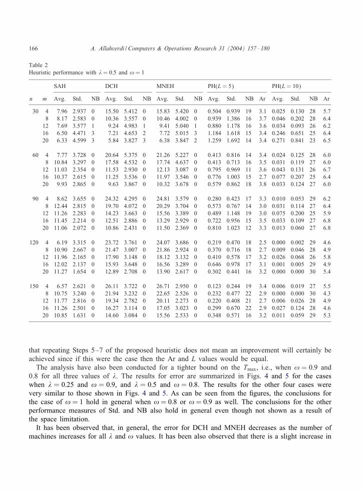
that repeating Steps 5–7 of the proposed heuristic does not mean an improvement will certainly beachieved since if this were the case then the Ar and L values would be equal.The analysis have also been conducted for a tighter bound on the Tmax, i.e., when ! = 0:9 and
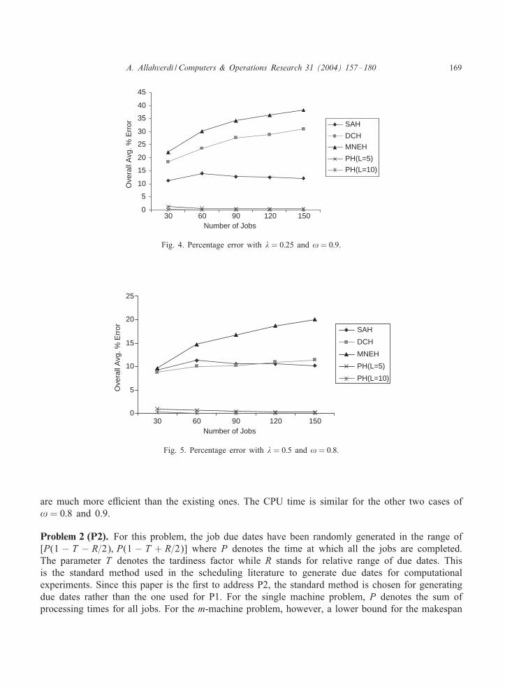
0.8 for all three values of �. The results for error are summarized in Figs. 4 and 5 for the caseswhen � = 0:25 and ! = 0:9, and � = 0:5 and ! = 0:8. The results for the other four cases werevery similar to those shown in Figs. 4 and 5. As can be seen from the 2gures, the conclusions forthe case of ! = 1 hold in general when ! = 0:8 or ! = 0:9 as well. The conclusions for the otherperformance measures of Std. and NB also hold in general even though not shown as a result ofthe space limitation.
It has been observed that, in general, the error for DCH and MNEH decreases as the number ofmachines increases for all � and ! values. It has been also observed that there is a slight increase in
A. Allahverdi / Computers & Operations Research 31 (2004) 157–180 167
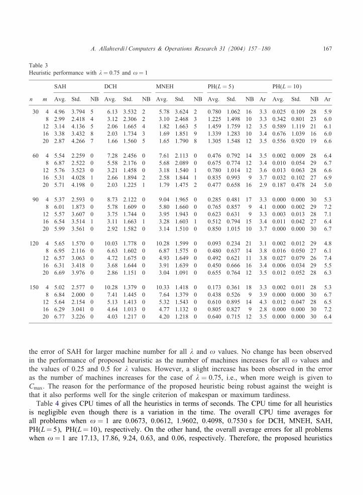
Table 3Heuristic performance with � = 0:75 and != 1
SAH DCH MNEH PH(L= 5) PH(L= 10)
n m Avg. Std. NB Avg. Std. NB Avg. Std. NB Avg. Std. NB Ar Avg. Std. NB Ar
30 4 4.96 3.794 5 6.13 3.532 2 5.78 3.624 2 0.780 1.062 16 3.3 0.025 0.109 28 5.98 2.99 2.418 4 3.12 2.306 2 3.10 2.468 3 1.225 1.498 10 3.3 0.342 0.801 23 6.012 3.14 4.136 5 2.06 1.665 4 1.82 1.663 5 1.459 1.759 12 3.5 0.589 1.119 21 6.116 3.38 3.432 8 2.03 1.734 3 1.69 1.851 9 1.339 1.283 10 3.4 0.676 1.039 16 6.020 2.87 4.266 7 1.66 1.560 5 1.65 1.790 8 1.305 1.548 12 3.5 0.556 0.920 19 6.6
60 4 5.54 2.259 0 7.28 2.456 0 7.61 2.113 0 0.476 0.792 14 3.5 0.002 0.009 28 6.48 6.87 2.522 0 5.58 2.176 0 5.68 2.089 0 0.675 0.774 12 3.4 0.010 0.054 29 6.712 5.76 3.523 0 3.21 1.458 0 3.18 1.540 1 0.780 1.014 12 3.6 0.013 0.063 28 6.616 5.31 4.028 1 2.66 1.894 2 2.58 1.844 1 0.835 0.993 9 3.7 0.032 0.102 27 6.920 5.71 4.198 0 2.03 1.225 1 1.79 1.475 2 0.477 0.658 16 2.9 0.187 0.478 24 5.0
90 4 5.37 2.593 0 8.73 2.122 0 9.04 1.965 0 0.285 0.481 17 3.3 0.000 0.000 30 5.38 6.01 1.873 0 5.78 1.609 0 5.80 1.660 0 0.765 0.857 9 4.1 0.000 0.002 29 7.212 5.57 3.607 0 3.75 1.744 0 3.95 1.943 0 0.623 0.631 9 3.3 0.003 0.013 28 7.116 6.54 3.514 1 3.11 1.663 1 3.28 1.603 1 0.512 0.794 15 3.4 0.011 0.042 27 6.420 5.99 3.561 0 2.92 1.582 0 3.14 1.510 0 0.850 1.015 10 3.7 0.000 0.000 30 6.7
120 4 5.65 1.570 0 10.03 1.778 0 10.28 1.599 0 0.093 0.234 21 3.1 0.002 0.012 29 4.88 6.95 2.116 0 6.63 1.602 0 6.87 1.575 0 0.480 0.637 14 3.8 0.016 0.050 27 6.112 6.57 3.063 0 4.72 1.675 0 4.93 1.649 0 0.492 0.621 11 3.8 0.027 0.079 26 7.416 6.31 3.418 0 3.68 1.644 0 3.91 1.639 0 0.450 0.666 16 3.4 0.006 0.034 29 5.520 6.69 3.976 0 2.86 1.151 0 3.04 1.091 0 0.655 0.764 12 3.5 0.012 0.052 28 6.3
150 4 5.02 2.577 0 10.28 1.379 0 10.33 1.418 0 0.173 0.361 18 3.3 0.002 0.011 28 5.38 6.84 2.000 0 7.41 1.445 0 7.64 1.379 0 0.438 0.526 9 3.9 0.000 0.000 30 6.712 5.64 2.154 0 5.13 1.413 0 5.32 1.543 0 0.610 0.895 14 4.3 0.012 0.047 28 6.516 6.29 3.041 0 4.64 1.013 0 4.77 1.132 0 0.805 0.827 9 2.8 0.000 0.000 30 7.220 6.77 3.226 0 4.03 1.217 0 4.20 1.218 0 0.640 0.715 12 3.5 0.000 0.000 30 6.4
the error of SAH for larger machine number for all � and ! values. No change has been observedin the performance of proposed heuristic as the number of machines increases for all ! values andthe values of 0.25 and 0.5 for � values. However, a slight increase has been observed in the erroras the number of machines increases for the case of � = 0:75, i.e., when more weigh is given toCmax. The reason for the performance of the proposed heuristic being robust against the weight isthat it also performs well for the single criterion of makespan or maximum tardiness.
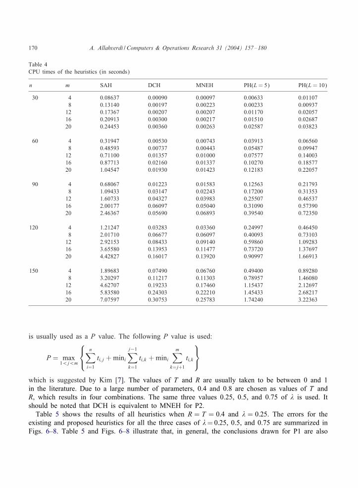
Table 4 gives CPU times of all the heuristics in terms of seconds. The CPU time for all heuristicsis negligible even though there is a variation in the time. The overall CPU time averages forall problems when ! = 1 are 0.0673, 0.0612, 1.9602, 0.4098, 0:7530 s for DCH, MNEH, SAH,PH(L=5); PH(L=10), respectively. On the other hand, the overall average errors for all problemswhen != 1 are 17.13, 17.86, 9.24, 0.63, and 0.06, respectively. Therefore, the proposed heuristics
168 A. Allahverdi / Computers & Operations Research 31 (2004) 157–180
0
5
10
15
20
25
30
35
40
45
30 60 90 120 150Number of Jobs
Ove
rall
Avg
. % E
rror SAH
DCH
MNEH
PH(L=5)
PH(L=10)
Fig. 1. Percentage error with � = 0:25 and != 1.
0
5
10
15
20
25
30 60 90 120 150Number of Jobs
Ove
rall
Avg
. % E
rror SAH
DCH
MNEH
PH(L=5)
PH(L=10)
Fig. 2. Percentage error with � = 0:5 and != 1.
0
1
2
3
4
5
6
7
30 60 90 120 150Number of Jobs
Ove
rall
Avg
. % E
rror SAH
DCH
MNEH
PH(L=5)
PH(L=10)
Fig. 3. Percentage error with � = 0:75 and != 1.
A. Allahverdi / Computers & Operations Research 31 (2004) 157–180 169
0
5
10
15
20
25
30
35
40
45
30 60 90 120 150Number of Jobs
Ove
rall
Avg
. % E
rror SAH
DCH
MNEH
PH(L=5)
PH(L=10)
Fig. 4. Percentage error with � = 0:25 and != 0:9.
0
5
10
15
20
25
30 60 90 120 150Number of Jobs
Ove
rall
Avg
. % E
rror SAH
DCH
MNEH
PH(L=5)
PH(L=10)
Fig. 5. Percentage error with � = 0:5 and != 0:8.
are much more e5cient than the existing ones. The CPU time is similar for the other two cases of!= 0:8 and 0.9.
Problem 2 (P2). For this problem, the job due dates have been randomly generated in the range of[P(1 − T − R=2); P(1 − T + R=2)] where P denotes the time at which all the jobs are completed.The parameter T denotes the tardiness factor while R stands for relative range of due dates. Thisis the standard method used in the scheduling literature to generate due dates for computationalexperiments. Since this paper is the 2rst to address P2, the standard method is chosen for generatingdue dates rather than the one used for P1. For the single machine problem, P denotes the sum ofprocessing times for all jobs. For the m-machine problem, however, a lower bound for the makespan
170 A. Allahverdi / Computers & Operations Research 31 (2004) 157–180
Table 4CPU times of the heuristics (in seconds)
n m SAH DCH MNEH PH(L= 5) PH(L= 10)
30 4 0.08637 0.00090 0.00097 0.00633 0.011078 0.13140 0.00197 0.00223 0.00233 0.0093712 0.17367 0.00207 0.00207 0.01170 0.0205716 0.20913 0.00300 0.00217 0.01510 0.0268720 0.24453 0.00360 0.00263 0.02587 0.03823
60 4 0.31947 0.00530 0.00743 0.03913 0.065608 0.48593 0.00737 0.00443 0.05487 0.0994712 0.71100 0.01357 0.01000 0.07577 0.1400316 0.87713 0.02160 0.01337 0.10270 0.1857720 1.04547 0.01930 0.01423 0.12183 0.22057
90 4 0.68067 0.01223 0.01583 0.12563 0.217938 1.09433 0.03147 0.02243 0.17200 0.3135312 1.60733 0.04327 0.03983 0.25507 0.4653716 2.00177 0.06097 0.05040 0.31090 0.5739020 2.46367 0.05690 0.06893 0.39540 0.72350
120 4 1.21247 0.03283 0.03360 0.24997 0.464508 2.01710 0.06677 0.06097 0.40093 0.7310312 2.92153 0.08433 0.09140 0.59860 1.0928316 3.65580 0.13953 0.11477 0.73720 1.3769720 4.42827 0.16017 0.13920 0.90997 1.66913
150 4 1.89683 0.07490 0.06760 0.49400 0.892808 3.20297 0.11217 0.11303 0.78957 1.4608012 4.62707 0.19233 0.17460 1.15437 2.1269716 5.83580 0.24303 0.22210 1.45433 2.6821720 7.07597 0.30753 0.25783 1.74240 3.22363
is usually used as a P value. The following P value is used:
P = max1¡j¡m
n∑i=1
ti; j +mini
j−1∑k=1
ti; k +minim∑
k=j+1
ti; k
which is suggested by Kim [7]. The values of T and R are usually taken to be between 0 and 1in the literature. Due to a large number of parameters, 0.4 and 0.8 are chosen as values of T andR, which results in four combinations. The same three values 0.25, 0.5, and 0.75 of � is used. Itshould be noted that DCH is equivalent to MNEH for P2.
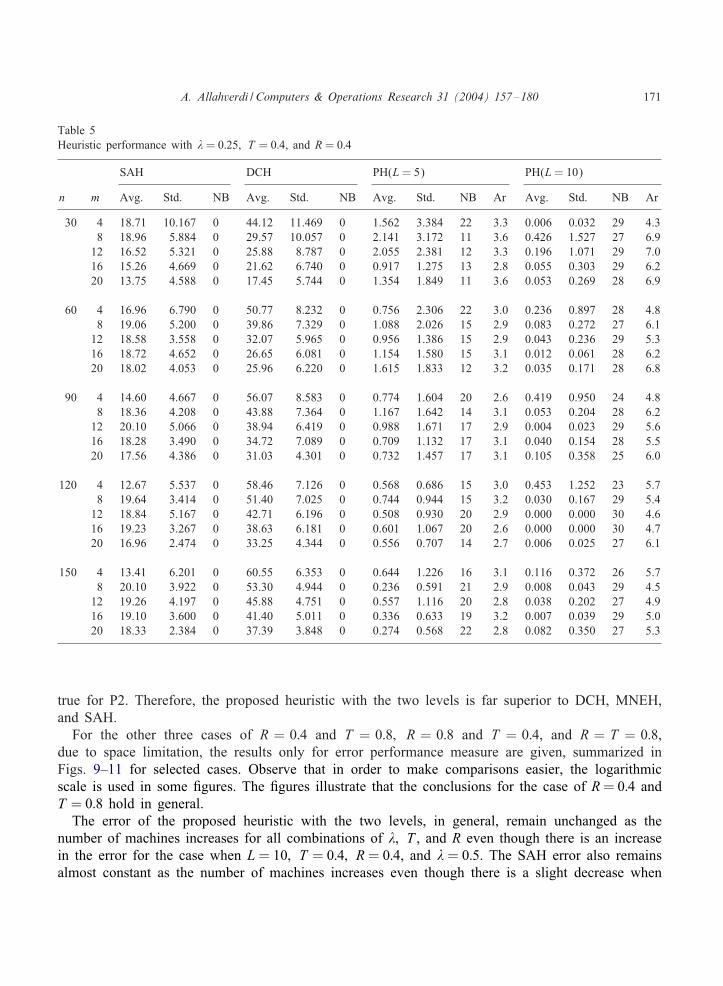
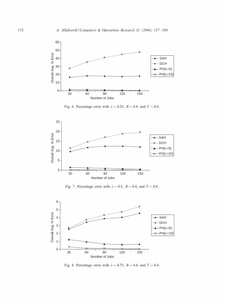
Table 5 shows the results of all heuristics when R = T = 0:4 and � = 0:25. The errors for theexisting and proposed heuristics for all the three cases of �=0:25, 0.5, and 0.75 are summarized inFigs. 6–8. Table 5 and Figs. 6–8 illustrate that, in general, the conclusions drawn for P1 are also
A. Allahverdi / Computers & Operations Research 31 (2004) 157–180 171
Table 5Heuristic performance with � = 0:25; T = 0:4, and R= 0:4
SAH DCH PH(L= 5) PH(L= 10)
n m Avg. Std. NB Avg. Std. NB Avg. Std. NB Ar Avg. Std. NB Ar
30 4 18.71 10.167 0 44.12 11.469 0 1.562 3.384 22 3.3 0.006 0.032 29 4.38 18.96 5.884 0 29.57 10.057 0 2.141 3.172 11 3.6 0.426 1.527 27 6.912 16.52 5.321 0 25.88 8.787 0 2.055 2.381 12 3.3 0.196 1.071 29 7.016 15.26 4.669 0 21.62 6.740 0 0.917 1.275 13 2.8 0.055 0.303 29 6.220 13.75 4.588 0 17.45 5.744 0 1.354 1.849 11 3.6 0.053 0.269 28 6.9
60 4 16.96 6.790 0 50.77 8.232 0 0.756 2.306 22 3.0 0.236 0.897 28 4.88 19.06 5.200 0 39.86 7.329 0 1.088 2.026 15 2.9 0.083 0.272 27 6.112 18.58 3.558 0 32.07 5.965 0 0.956 1.386 15 2.9 0.043 0.236 29 5.316 18.72 4.652 0 26.65 6.081 0 1.154 1.580 15 3.1 0.012 0.061 28 6.220 18.02 4.053 0 25.96 6.220 0 1.615 1.833 12 3.2 0.035 0.171 28 6.8
90 4 14.60 4.667 0 56.07 8.583 0 0.774 1.604 20 2.6 0.419 0.950 24 4.88 18.36 4.208 0 43.88 7.364 0 1.167 1.642 14 3.1 0.053 0.204 28 6.212 20.10 5.066 0 38.94 6.419 0 0.988 1.671 17 2.9 0.004 0.023 29 5.616 18.28 3.490 0 34.72 7.089 0 0.709 1.132 17 3.1 0.040 0.154 28 5.520 17.56 4.386 0 31.03 4.301 0 0.732 1.457 17 3.1 0.105 0.358 25 6.0
120 4 12.67 5.537 0 58.46 7.126 0 0.568 0.686 15 3.0 0.453 1.252 23 5.78 19.64 3.414 0 51.40 7.025 0 0.744 0.944 15 3.2 0.030 0.167 29 5.412 18.84 5.167 0 42.71 6.196 0 0.508 0.930 20 2.9 0.000 0.000 30 4.616 19.23 3.267 0 38.63 6.181 0 0.601 1.067 20 2.6 0.000 0.000 30 4.720 16.96 2.474 0 33.25 4.344 0 0.556 0.707 14 2.7 0.006 0.025 27 6.1
150 4 13.41 6.201 0 60.55 6.353 0 0.644 1.226 16 3.1 0.116 0.372 26 5.78 20.10 3.922 0 53.30 4.944 0 0.236 0.591 21 2.9 0.008 0.043 29 4.512 19.26 4.197 0 45.88 4.751 0 0.557 1.116 20 2.8 0.038 0.202 27 4.916 19.10 3.600 0 41.40 5.011 0 0.336 0.633 19 3.2 0.007 0.039 29 5.020 18.33 2.384 0 37.39 3.848 0 0.274 0.568 22 2.8 0.082 0.350 27 5.3
true for P2. Therefore, the proposed heuristic with the two levels is far superior to DCH, MNEH,and SAH.
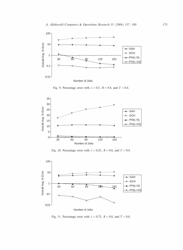
For the other three cases of R = 0:4 and T = 0:8; R = 0:8 and T = 0:4, and R = T = 0:8,due to space limitation, the results only for error performance measure are given, summarized inFigs. 9–11 for selected cases. Observe that in order to make comparisons easier, the logarithmicscale is used in some 2gures. The 2gures illustrate that the conclusions for the case of R= 0:4 andT = 0:8 hold in general.The error of the proposed heuristic with the two levels, in general, remain unchanged as the
number of machines increases for all combinations of �; T , and R even though there is an increasein the error for the case when L= 10; T = 0:4; R= 0:4, and � = 0:5. The SAH error also remainsalmost constant as the number of machines increases even though there is a slight decrease when
172 A. Allahverdi / Computers & Operations Research 31 (2004) 157–180
0
10
20
30
40
50
60
30 60 90 120 150Number of Jobs
Ove
rall
Avg
. % E
rror
SAH
DCH
PH(L=5)
PH(L=10)
Fig. 6. Percentage error with � = 0:25; R= 0:4, and T = 0:4.
0
5
10
15
20
25
30 60 90 120 150Number of Jobs
Ove
rall
Avg
. % E
rror
SAH
DCH
PH(L=5)
PH(L=10)
Fig. 7. Percentage error with � = 0:5; R= 0:4, and T = 0:4.
0
1
2
3
4
5
6
30 60 90 120 150Number of Jobs
Ove
rall
Avg
. % E
rror
SAH
DCH
PH(L=5)
PH(L=10)
Fig. 8. Percentage error with � = 0:75; R= 0:4, and T = 0:4.
A. Allahverdi / Computers & Operations Research 31 (2004) 157–180 173
0.01
0.1
1
10
100
30 60 90 120 150
Number of Jobs
Ove
rall
Avg
. % E
rror
SAH
DCH
PH(L=5)
PH(L=10)
Fig. 9. Percentage error with � = 0:5; R= 0:8, and T = 0:4.
0
5
10
15
20
25
30
35
30 60 90 120 150Number of Jobs
Ove
rall
Avg
. % E
rror
SAH
DCH
PH(L=5)
PH(L=10)
Fig. 10. Percentage error with � = 0:25; R= 0:8, and T = 0:4.
0.01
0.1
1
10
100
30 60 90 120 150
Number of Jobs
Ove
rall
Avg
. % E
rror
SAH
DCH
PH(L=5)
PH(L=10)
Fig. 11. Percentage error with � = 0:75; R= 0:8, and T = 0:8.
174 A. Allahverdi / Computers & Operations Research 31 (2004) 157–180
Table 6Evaluation of the dominance relation for the three-machine problem
n T = 0:4 T = 0:8 T = 0:4 T = 0:8R= 0:4 R= 0:4 R= 0:8 R= 0:8
5 37.13 41.01 41.92 38.416 50.82 52.87 54.95 55.627 57.28 59.98 62.10 58.238 59.25 65.05 74.87 68.879 66.21 67.87 71.37 72.0910 78.32 78.12 84.92 82.4211 79.74 78.99 90.12 90.3212 85.78 82.77 92.66 93.45
�= 0:75 for the two combinations of T = 0:4 and R= 0:4, and T = 0:4 and R= 0:8. The errors forDCH and MNEH decrease as the number of machines increases for all �; T , and R combinations.
The CPU time for all the heuristics is again negligible, which is similar to the one for P1.
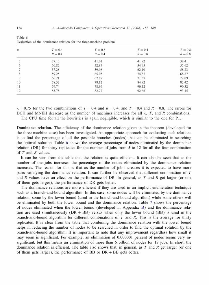
Dominance relation. The e5ciency of the dominance relation given in the theorem (developed forthe three-machine case) has been investigated. An appropriate approach for evaluating such relationsis to 2nd the percentage of all the possible branches (nodes) that can be eliminated in searchingthe optimal solution. Table 6 shows the average percentage of nodes eliminated by the dominancerelation (DR) for thirty replicates for the number of jobs from 5 to 12 for all the four combinationof T and R values.It can be seen from the table that the relation is quite e5cient. It can also be seen that as the
number of the jobs increases the percentage of the nodes eliminated by the dominance relationincreases. The reason for this is that as the number of job increases it is expected to have morepairs satisfying the dominance relation. It can further be observed that diMerent combination of Tand R values have an eMect on the performance of DR. In general, as T and R get larger (or oneof them gets larger), the performance of DR gets better.
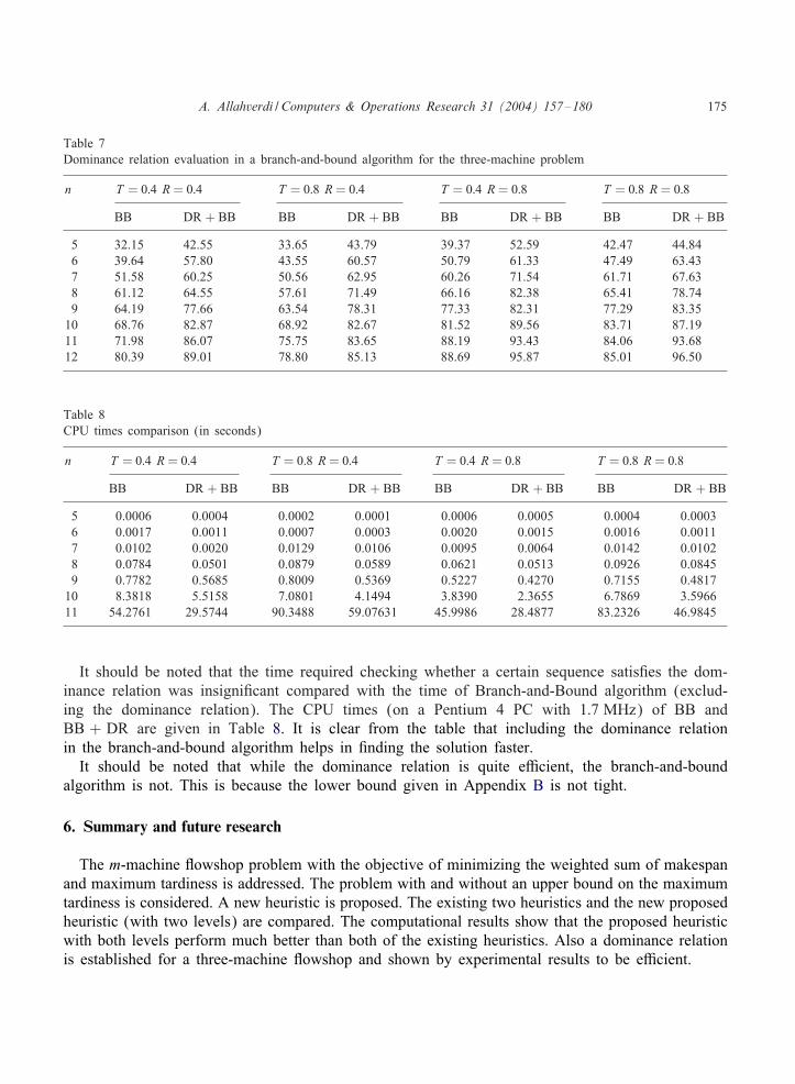
The dominance relations are more e5cient if they are used in an implicit enumeration techniquesuch as a branch-and-bound algorithm. In this case, some nodes will be eliminated by the dominancerelation, some by the lower bound (used in the branch-and-bound algorithm) while some others willbe eliminated by both the lower bound and the dominance relation. Table 7 shows the percentageof nodes eliminated when the lower bound (developed in Appendix B) and the dominance rela-tion are used simultaneously (DR + BB) versus when only the lower bound (BB) is used in thebranch-and-bound algorithm for diMerent combinations of T and R. This is the average for thirtyreplicates. It is clear from the table that combining the dominance relation with the lower boundhelps in reducing the number of nodes to be searched in order to 2nd the optimal solution by thebranch-and-bound algorithm. It is important to note that any improvement regardless how small itmay seem is signi2cant. For example, an elimination of 0.000001 percent of nodes seems very in-signi2cant, but this means an elimination of more than 6 billion of nodes for 18 jobs. In short, thedominance relation is e5cient. The table also shows that, in general, as T and R get larger (or oneof them gets larger), the performance of BB or DR + BB gets better.
A. Allahverdi / Computers & Operations Research 31 (2004) 157–180 175
Table 7Dominance relation evaluation in a branch-and-bound algorithm for the three-machine problem
n T = 0:4 R= 0:4 T = 0:8 R= 0:4 T = 0:4 R= 0:8 T = 0:8 R= 0:8
BB DR + BB BB DR + BB BB DR + BB BB DR + BB
5 32.15 42.55 33.65 43.79 39.37 52.59 42.47 44.846 39.64 57.80 43.55 60.57 50.79 61.33 47.49 63.437 51.58 60.25 50.56 62.95 60.26 71.54 61.71 67.638 61.12 64.55 57.61 71.49 66.16 82.38 65.41 78.749 64.19 77.66 63.54 78.31 77.33 82.31 77.29 83.3510 68.76 82.87 68.92 82.67 81.52 89.56 83.71 87.1911 71.98 86.07 75.75 83.65 88.19 93.43 84.06 93.6812 80.39 89.01 78.80 85.13 88.69 95.87 85.01 96.50
Table 8CPU times comparison (in seconds)
n T = 0:4 R= 0:4 T = 0:8 R= 0:4 T = 0:4 R= 0:8 T = 0:8 R= 0:8
BB DR + BB BB DR + BB BB DR + BB BB DR + BB
5 0.0006 0.0004 0.0002 0.0001 0.0006 0.0005 0.0004 0.00036 0.0017 0.0011 0.0007 0.0003 0.0020 0.0015 0.0016 0.00117 0.0102 0.0020 0.0129 0.0106 0.0095 0.0064 0.0142 0.01028 0.0784 0.0501 0.0879 0.0589 0.0621 0.0513 0.0926 0.08459 0.7782 0.5685 0.8009 0.5369 0.5227 0.4270 0.7155 0.481710 8.3818 5.5158 7.0801 4.1494 3.8390 2.3655 6.7869 3.596611 54.2761 29.5744 90.3488 59.07631 45.9986 28.4877 83.2326 46.9845
It should be noted that the time required checking whether a certain sequence satis2es the dom-inance relation was insigni2cant compared with the time of Branch-and-Bound algorithm (exclud-ing the dominance relation). The CPU times (on a Pentium 4 PC with 1:7 MHz) of BB andBB + DR are given in Table 8. It is clear from the table that including the dominance relationin the branch-and-bound algorithm helps in 2nding the solution faster.
It should be noted that while the dominance relation is quite e5cient, the branch-and-boundalgorithm is not. This is because the lower bound given in Appendix B is not tight.
6. Summary and future research
The m-machine &owshop problem with the objective of minimizing the weighted sum of makespanand maximum tardiness is addressed. The problem with and without an upper bound on the maximumtardiness is considered. A new heuristic is proposed. The existing two heuristics and the new proposedheuristic (with two levels) are compared. The computational results show that the proposed heuristicwith both levels perform much better than both of the existing heuristics. Also a dominance relationis established for a three-machine &owshop and shown by experimental results to be e5cient.
176 A. Allahverdi / Computers & Operations Research 31 (2004) 157–180
The given lower bound is not e5cient, and hence, a possible extension to this paper is to searchfor a better lower bound and use this lower bound along with the dominance relation given in thispaper in a branch-and-bound algorithm.
The existing heuristics DCH and SAH and the proposed heuristic are developed for the environ-ments where setup times are neglected or included in the processing times. While this assumptionmight be valid for some environments there are some other environments in which the assumption isnot valid. An important implication of separate setup times is that the setup on a subsequent machinemay be performed while the job is still in process on the immediately preceding machine. This willimprove machine utilization and may reduce completion time. Allahverdi et al. [15] provide a recentsurvey paper on scheduling problems with separate setup times. The problem with separate setuptimes has been addressed in the literature for the individual criterion of makespan (e.g., Yoshida andHitomi [16], and Allahverdi [17]) or maximum lateness [18] for the two-machine case. A possibleand natural extension for this paper is to consider a two-machine (or m-machine) &owshop problemof minimizing a weighted sum of makespan and maximum tardiness (lateness) where setup timesare treated as separate.
Acknowledgements
I would like to thank unanimous referees for their valuable suggestions and comments, whichconsiderably improved the paper.
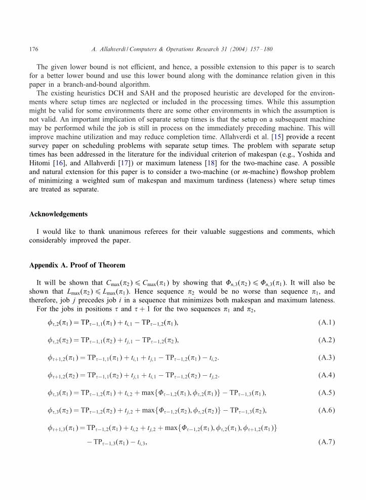
Appendix A. Proof of Theorem
It will be shown that Cmax(�2)6Cmax(�1) by showing that �n;3(�2)6�n;3(�1). It will also beshown that Lmax(�2)6Lmax(�1). Hence sequence �2 would be no worse than sequence �1, andtherefore, job j precedes job i in a sequence that minimizes both makespan and maximum lateness.For the jobs in positions � and �+ 1 for the two sequences �1 and �2,
��;2(�1) = TP�−1;1(�1) + ti;1 − TP�−1;2(�1); (A.1)
��;2(�2) = TP�−1;1(�2) + tj;1 − TP�−1;2(�2); (A.2)
��+1;2(�1) = TP�−1;1(�1) + ti;1 + tj;1 − TP�−1;2(�1)− ti;2: (A.3)
��+1;2(�2) = TP�−1;1(�2) + tj;1 + ti;1 − TP�−1;2(�2)− tj;2: (A.4)
��;3(�1) = TP�−1;2(�1) + ti;2 + max{��−1;2(�1); ��;2(�1)} − TP�−1;3(�1); (A.5)
��;3(�2) = TP�−1;2(�2) + tj;2 + max{��−1;2(�2); ��;2(�2)} − TP�−1;3(�2); (A.6)
��+1;3(�1) = TP�−1;2(�1) + ti;2 + tj;2 + max{��−1;2(�1); ��;2(�1); ��+1;2(�1)}−TP�−1;3(�1)− ti;3; (A.7)
A. Allahverdi / Computers & Operations Research 31 (2004) 157–180 177
��+1;3(�2) = TP�−1;2(�2) + tj;2 + ti;2 + max{��−1;2(�2); ��;2(�2); ��+1;2(�2)}−TP�−1;3(�2)− tj;3: (A.8)
Observe that in Eqs. (A.1)–(A.8), TP�−1; k(�1) = TP�−1; k(�2) for k = 1; 2; 3 since both sequenceshave the same jobs in all positions prior to �.
It follows from Eqs. (A.1), (A.2), (A.5), and (A.6) and condition (iia) of the Theorem that
��;3(�2)6��;3(�1) and ��;2(�2)6��;2(�1): (A.9)
From Eqs. (A.1)–(A.3), (A.6) and (A.7) and condition (iib) of the Theorem,
��;3(�2)6��+1;3(�1) and either ��;2(�2)6��;2(�1) or ��;2(�2)6��+1;2(�1): (A.10)
If condition (iiia) of the Theorem holds, then from Eqs. (A.2), (A.4), (A.6), and (A.8),
��+1;3(�2)6��;3(�2) and ��+1;2(�2)6��;2(�2): (A.11)
On the other hand, if condition (iiib) of the Theorem holds, then from Eqs. (A.1), (A.2), (A.4),(A.5) and (A.8),
��+1;3(�2)6��;3(�1) and either ��+1;2(�2)6��;2(�2) or ��+1;2(�2)6��;2(�1): (A.12)
Finally, if condition (iiic) of the Theorem holds, then from Eqs. (A.1), (A.2), (A.4), (A.7) and(A.8),
��+1;3(�2)6��+1;3(�1) and either ��+1;2(�2)6��;2(�2) or
��+1;2(�2)6��;2(�1): (A.13)
Now if one of Eqs. (A.9) or (A.10) and any one of Eqs. (A.11), (A.12), or (A.13) hold then
max{��;2(�2); ��+1;2(�2)}6max{��;2(�1); ��+1;2(�1)}; (A.14)
max{��;3(�2); ��+1;3(�2)}6max{��;3(�1); ��+1;3(�1)}: (A.15)
Therefore, by Lemma 2 and Eqs. (A.14) and (A.15)
�n;3(�2)6�n;3(�1) or equivalently Cmax(�2)6Cmax(�1):
For sequences �1 and �2, the lateness of the jobs in positions � and �+ 1 are given as
L�(�2) = TP�−1;3(�2) + tj;3 + max{��−1;3(�2); ��;3(�2)} − dj;
L�+1(�1) = TP�−1;3(�1) + ti;3 + tj;3 + max{��−1;3(�1); ��;3(�1); ��+1;3(�1)} − dj
and
L�+1(�2) = TP�−1;3(�2) + tj;3 + ti;3 + max{��−1;3(�2); ��;3(�2); ��+1;3(�2)} − di:
From the last three equations and the condition (i) of the Theorem, and if one of Eq. (A.9) or(A.10) holds,
L�(�2)6L�+1(�1) and L�+1(�2)6L�+1(�1): (A.16)
Lmax(�2)6Lmax(�1) follows from Eqs. (A.14)–(A.16), and Lemma 3.This concludes the proof.
178 A. Allahverdi / Computers & Operations Research 31 (2004) 157–180
Appendix B. A lower bound
Let ! represent the set of jobs already assigned (assume ‘ jobs are assigned) and # represent theset of jobs to be assigned (n − ‘). Order the jobs in the set # in non-decreasing order of ti; j, andlet t[i; j] denote the ith smallest ti; j. It is not hard to see that for j¿‘,
C[j;3]¿‘∑i=1
t[i;1] +j−‘∑i=1i∈#
t[i;1] + mini∈#
(ti;2) + mini∈#
(ti;3);
C[j;3]¿C[‘;2] +j−‘∑i=1i∈#
t[i;2] + mini∈#
(ti;3);
and
C[j;3]¿C[‘;3] +j−‘∑i=1i∈#
t[i;3] where0∑r=1
(:) = 0:
Thus, from the above three inequalities
C[j;3]¿max
‘∑i=1
t[i;1] +j−‘∑i=1i∈#
t[i;1] + mini∈#
(ti;2) + mini∈#
(ti;3);
C[‘;2] +j−‘∑i=1i∈#
t[i;2] + mini∈#
(ti;3); C[‘;3] +j−‘∑i=1i∈#
t[i;3]
:
Given a lower bound on the completion time of the job in position j, then a lower bound on themakespan can be established by
LB(Cmax) = max{C[1;3]; C[2;3]; : : : ; C[n;3]}:A lower bound on the tardiness of the job in position j (j¿‘) is obtained by
T[j]¿max
max
‘∑i=1
t[i;1] +j−‘∑i=1i∈#
t[i;1] + mini∈#
(ti;2) + mini∈#
(ti;3);
A. Allahverdi / Computers & Operations Research 31 (2004) 157–180 179
C[‘;2] +j−‘∑i=1i∈#
t[i;2] + mini∈#
(ti;3); C[‘;3] +j−‘∑i=1i∈#
t[i;3]
−maxi∈#
(di); 0
:
Therefore, a lower bound on Tmax is given as
LB(Tmax) = max{T[1]; T[2]; : : : ; T[n]}:Now, a lower bound on the objective function value (OFV) can be constructed by the followingequation:
LB(OFV) = �LB(Cmax) + (1− �) LB(Tmax):
References
[1] Nawaz M, Enscore E, Ham I. A heuristic algorithm for the m-machine, n-job &owshop sequencing problem. OMEGAThe International Journal of Management Sciences 1983;11:91–5.
[2] Chu C, Proth JM, Sethi S. Heuristic procedures for minimizing makespan and the number of required pallets.European Journal of Operational Research 1995;86:491–502.
[3] Zegordi SH, Itoh K, Enkawa T. Minimizing makespan for &ow shop scheduling by combining simulated annealingwith sequencing knowledge. European Journal of Operational Research 1995;85:515–31.
[4] Riane F, Artiba A, Elmaghraby SE. A hybrid three-stage &owshop problem: e5cient heuristics to minimize makespan.European Journal of Operational Research 1998;109:321–9.
[5] Townsend W. Sequencing n jobs on m machines to minimize maximum tardiness: a branch-and-bound solution.Management Science 1977;23:1016–9.
[6] Kim YD. Heuristics for &owshop scheduling problems minimizing mean tardiness. Journal of the OperationalResearch Society 1993;44:19–28.
[7] Kim YD. Minimizing total tardiness in permutation &owshops. European Journal of Operational Research 1995;85:541–55.
[8] Srinivasaraghavan P, Rajendran C. Scheduling to minimize mean tardiness and weighted mean tardiness in &owshopand &owline-based manufacturing cell. Computers and Industrial Engineering 1998;34:531–46.
[9] Armentano VA, Ronconi DP. Tabu search for total tardiness minimization in &owshop scheduling problems.Computers and Operations Research 1999;26:219–35.
[10] Nagar A, Haddock J, Heragu S. Multiple and bicriteria scheduling: a literature review. European Journal ofOperational Research 1995;81:88–104.
[11] Daniels RL, Chambers RJ. Multiobjective &ow-shop scheduling. Naval Research Logistics 1990;37:981–95.[12] Chakravarthy K, Rajendran C. A heuristic for scheduling in a &owshop with the bicriteria of makespan and maximum
tardiness minimization. Production Planning and Control 1999;10:707–14.[13] Rajendran C, Ziegler H. An e5cient heuristic for scheduling in a &owshop to minimize total weighted &owtime of
jobs. European Journal of Operational Research 1997;103:129–38.[14] Woo HS, Yim DS. A heuristic algorithm for mean &owtime objective in &owshop scheduling. Computers and
Operations Research 1998;25:175–82.[15] Allahverdi A, Gupta JND, Aldowiasan TA. A review of scheduling research involving setup considerations. OMEGA
The International Journal of Management Sciences 1999;27:219–39.[16] Yoshida T, Hitomi K. Optimal two-stage production scheduling with setup times separated. AIIE Transactions
1979;11:261–3.
180 A. Allahverdi / Computers & Operations Research 31 (2004) 157–180
[17] Allahverdi A. Two-stage production scheduling with separated setup times and stochastic breakdowns. Journal of theOperational Research Society 1995;46:896–904.
[18] Dileepan P, Sen T. Job lateness in a two-machine &owshop with setup times separated. Computers and OperationsResearch 1991;18:549–56.
Ali Allahverdi is an Associate Professor in the Department of Industrial and Management Systems Engineering of KuwaitUniversity. He received his B.S. in Petroleum Engineering from Istanbul Technical University and his M.Sc. and Ph.D. inIndustrial Engineering, from Rensselaer Polytechnic Institute, New York. His current research interests include schedulingand modular production. He has published numerous articles in Computers and Operations Research, European Journal ofOperational Research, Journal of the Operational Research Society, International Transactions in Operational Research,International Journal of Industrial Engineering, and Computers and Industrial Engineering. He has also published articlesin Naval Research Logistics, OMEGA The International Journal of Management Science, International Journal ofProduction Economics, Mathematical and Computer Modeling, Journal of Intelligent Manufacturing, InternationalJournal of Parallel and Distributed Systems, and Communications in Statistics: Simulation and Computation.