Embed Size (px)
Citation preview
Alma Mater Studiorum – Università di Bologna
DOTTORATO DI RICERCA
MODELLISTICA FISICA PER LA PROTEZIONE
dell’AMBIENTE
Ciclo XX
Settore scientifico disciplinari di afferenza: FIS/06
A NEW SNOWFALL DETECTION ALGORITHM FOR
HIGH LATITUDE REGIONS BASED
ON A COMBINATION OF ACTIVE AND PASSIVE
SENSORS
Presentata da:
Dott. Ing. Giulio Todini
Coordinatore Dottorato: Relatore:
Professor Ezio Todini Professor Rolando Rizzi
Esame finale anno 2008
2
ABSTRACT
Precipitation retrieval over high latitudes, particularly snowfall retrieval over ice and snow, using
satellite-based passive microwave spectrometers, is currently an unsolved problem. The challenge
results from the large variability of microwave emissivity spectra for snow and ice surfaces, which
can mimic, to some degree, the spectral characteristics of snowfall.
This work focuses on the investigation of a new snowfall detection algorithm specific for high
latitude regions, based on a combination of active and passive sensors able to discriminate between
snowing and non snowing areas.
The space-borne Cloud Profiling Radar (on CloudSat), the Advanced Microwave Sensor units A
and B (on NOAA-16) and the infrared spectrometer MODIS (on AQUA) have been co-located for
365 days, from October 1st 2006 to September 30
th, 2007.
CloudSat products have been used as truth to calibrate and validate all the proposed algorithms.
The methodological approach followed can be summarised into two different steps.
In a first step, an empirical search for a threshold, aimed at discriminating the case of no snow, was
performed, following Kongoli et al. [2003]. This single-channel approach has not produced
appropriate results, a more statistically sound approach was attempted.
Two different techniques, which allow to compute the probability above and below a Brightness
Temperature (BT) threshold, have been used on the available data. The first technique is based upon
a Logistic Distribution to represent the probability of Snow given the predictors. The second
technique, defined Bayesian Multivariate Binary Predictor (BMBP), is a fully Bayesian technique
not requiring any hypothesis on the shape of the probabilistic model (such as for instance the
Logistic), which only requires the estimation of the BT thresholds.
The results obtained show that both methods proposed are able to discriminate snowing and non
snowing condition over the Polar regions with a probability of correct detection larger than 0.5,
highlighting the importance of a multispectral approach.
3
INDEX:
1 INTRODUCTION ................................................................................................................. 6
2 EXTENSION OF LBLMS TO THE MICROWAVE REGION ............................................... 8
2.1 LBLMS ............................................................................................................................. 8
2.1.1 GENPROF ............................................................................................................... 9
2.1.2 SPECTRO & HARTCODE .................................................................................... 10
2.1.3 MIESCAT .............................................................................................................. 12
2.1.4 RTX-3-input ........................................................................................................... 15
2.1.5 RTX-3 .................................................................................................................... 16
2.2 MICROWAVE REMOTE SENSING ............................................................................... 18
2.2.1 Gaseous line by line optical properties .................................................................... 18
2.2.2 Water Vapour Absorption and continuum ................................................................ 19
2.2.3 Oxygen absorption ................................................................................................. 20
2.2.4 Nitrogen absorption ................................................................................................ 21
2.2.5 Particles Optical Properties ..................................................................................... 21
2.3 TBARRAY AND TBSCAT .............................................................................................. 22
2.3.1 Water vapour absorption ......................................................................................... 22
2.3.2 Scattering ............................................................................................................... 23
2.4 LBLMS IMPLEMENTATIONS ...................................................................................... 25
2.4.1 Gaseous line by line optical properties .................................................................... 25
2.4.2 Scattering ............................................................................................................... 29
2.5 DISCUSSION ................................................................................................................. 30
3 APPLICATION OF THE NEW LBLMS TO THE CASE STUDIES .................................... 31
3.1 DATA SET PRESENTATION ......................................................................................... 31
3.1.1 GROUND BASED SENSORS ............................................................................... 32
3.1.2 SPACE-BORN INSTRUMENTS ........................................................................... 35
3.2 GROUND BASED SENSORS SIMULATIONS ............................................................. 37
3.2.1 Case study 1: Clear sky conditions ......................................................................... 37
3.2.2 Case study 2: Cloudy conditions ............................................................................. 47
3.3 SPACE BORN SENSORS SIMULATIONS .................................................................... 55
3.3.1 SURFACE MODEL ............................................................................................... 55
3.4 DISCUSSION ................................................................................................................. 62
4 A FIRST TENTATIVE: IMPROVING THE SSA ALGORITHM ......................................... 63
4.1 SSA ................................................................................................................................. 64
4
4.1.2 A METHOD TO DETECT FALSE ALARMS ........................................................ 64
4.1.3 DISCUSSION ........................................................................................................ 66
5 DEFINING AN ALTERNATIVE APPROACH: MATERIALS AND METHODS ................ 67
5.1 THE DATA USED TO IMPLEMENT THE APPROACH ................................................ 67
5.2 THE METHODOLOGICAL APPROACH ......................................................... 67
5.3 THE USED VERIFICATION CRITERIA ......................................................... 68
6 THE USED DATA AND THE CASE STUDIES .................................................................. 70
6.1 THE CLOUD PROFILING RADAR ............................................................................... 70
6.1.1 2B-CLDCLASS-Lidar ............................................................................................ 71
6.1.2 MODIS-AUX ......................................................................................................... 74
6.2 AMSU- CPR CO-LOCATION METHODOLOGY ......................................................... 75
6.2.3 DATA PRESENTATION ........................................................................................ 77
6.2.4 AMSU-B FOV ANALYSIS .................................................................................... 79
7 THE NEW APPROACH AND ITS APPLICATION ............................................................. 81
7.1 EMPIRICAL ANALYSIS ................................................................................................ 81
7.1.1 South Pole Winter over Land (SWL) ...................................................................... 84
7.1.2 South Pole Winter over Ocean (SWO) .................................................................... 86
7.1.3 South Pole Summer over Land(SSL) ...................................................................... 86
7.1.4 South Pole Summer over Ocean (SSO) ................................................................... 87
7.1.5 North Pole Winter over Land (NWL)...................................................................... 87
7.1.6 North Pole Winter over Ocean (NOW) ................................................................... 87
7.1.7 North Pole summer Over Land (NSL) .................................................................... 88
7.1.8 North Pole summer over ocean (NSO) .................................................................... 89
7.1.9 DISCUSSION ........................................................................................................ 89
7.2 COMBINING DIFFERENT MEASUREMENTS AND MODELS IN ORDER TO
IMPROVE PREDICTABILITY ............................................................................................... 90
7.2.1 Continuous Probability Problems: the Bayesian Model Averaging .......................... 91
7.2.2 Discrete Probability Problems: the Binary Response Models .................................. 93
7.3 A PURELY PROBABILISTIC APPROACH ................................................................... 95
7.3.1 The single predictor case: Bayesian Univariate Binary Predictor (BUBP) ............... 96
7.3.2 The multi-predictor case: Bayesian Multivariate Binary Predictor (BMBP) .......... 101
7.4 EXAMPLES OF APPLICATION .................................................................................. 104
7.4.1 South Pole Winter over Land ................................................................................ 106
7.4.2 South Pole Winter over Ocean .............................................................................. 107
7.4.3 South Pole Summer over Land ............................................................................. 108
5
7.4.4 North Pole Winter over Land ................................................................................ 109
7.4.5 North Pole Winter over Ocean .............................................................................. 110
7.4.6 North Pole Summer over Land .............................................................................. 111
7.4.7 North Pole Summer over Ocean ........................................................................... 112
7.5 DISCUSSION ............................................................................................................... 113
8 CONCLUSIONS ............................................................................................................... 115
References .................................................................................................................................. 117
Appendix A ................................................................................................................................. 125
AKNOWLEDGEMENTS ........................................................................................................... 127
6
1 INTRODUCTION
In high latitudes, a substantial portion of precipitation falls in the form of snow. Measuring snow
precipitation has many applications such as forecasting hazardous weather, understanding
hydrological water budget, and thus accurate estimates of precipitation on a global scale. As
reported by Mugnai et al. [2007], the yearly precipitation average over the Earth is about 690 mm,
about 5 % of which in the form of snowfall. Since snowfall is a significant portion of the total
precipitation amount, in Asia, northern regions of Europe, and North America, it becomes the main
driver of the regional and global water cycle process.
Although falling snow is such an important component of global precipitation at high latitude an
accurate estimation of the snowfall is not yet available. In fact ground-based snowfall
measurements are difficult to make due to strong wind effects on snow gauges and
melting/evaporating before measuring, and observation sites are very sparse in remote regions.
Therefore polar orbiting satellite measurements are a fundamental tool for snowfall observation on
high latitude regions, observing both polar regions every 90 minutes, and giving the opportunity to
have an accurate mapping of those areas.
Although satellite data have been extensively used in many cloud and rainfall studies, existing
satellite remote sensing techniques are not able to provide accurate snowfall retrievals, in particular
on ice and snow covered surfaces. Observation of snowfall from satellite is in fact hampered by the
lack of contrast between the snowfall spectral signature and the surface one for most of the remote
sensors used in current satellites. Because of this snowfall retrievals over land or sea-ice represent
an enormous challenge.
Numerous recent studies [Katsumata et al., 2000; Liu and Katsumata, 2002; Bennartz and Petty,
2001; Liu and Curry, 1997; Ferraro et al., 2000; Ferraro and Grody, 2001;Wang et al., 2001; Staelin
and Chen, 2000] have demonstrated the potential for more accurate precipitation retrievals
including snowfall utilizing higher frequency channels. Higher frequency channels are less
susceptible to the high variability in land surface emissivity, and still respond to the scattering
signatures due to precipitation [e.g., Skofronick-Jackson et al., 2002]. However all the methods
proposed have not be validated on Polar regions because of the lack of radar or rain gauges
observations. This has hampered, up to now, a positive evolution of algorithms specific for those
areas.
The launch in 2006 of a Cloud Profiling Radar, as part of the constellation A-Train, has been
identified as a possible answer to this need. The CPR provides new useful information, also in
region as the Poles, supplying daily cloud classification and presence of precipitation not available
7
previously.
This thesis proposes a new snowfall detection algorithm to discriminate between snowing and non
snowing condition on Polar regions .
To implement the new approach, the AMSU-A and B microwave observations from NOAA-16,
have been complemented by infrared data collected by MODIS on board of AQUA.
Two methods are proposed. The first method is based on a Logistic Distribution to represent the
probability of snow given the predictors while the second technique is a fully Bayesian technique
not requiring the hypothesis on the shape of the probabilistic model (such as for instance the
Logistic), which only requires the estimation of Brightness Temperature thresholds. Both the
techniques combine microwave and infrared channels, and they have been calibrated and validated
using CPR observations.
8
2 EXTENSION OF LBLMS TO THE MICROWAVE REGION
The Atmospheric Dynamic Group Bologna, in the last few years, has been working on a unique
suite of codes able to simulate energy fluxes and radiances in the spectral range from the visible to
the microwave. The goal of the group lead by Professor Rizzi, is to extend its expertise in the
infrared region to the short-wave and to the millimeter and sub-millimeter wavelengths in order to
use a same forward model for a retrieval methodology.
Satellite constellations, as the A-train, are an example of the new data set available with active and
passive observations from microwave to visible spectrum with a very short time lag produced for
the same area. A new accurate methodology for retrieving cloud optical and microphysical
properties using the full wave-number spectrum seems to be a fundamental tool.
The first part of this PhD work has been focused on the extension of the ADGB infrared model,
LBLMS, to the microwave region.
In this chapter the LBLMS model will be briefly presented. Next a review of the current state and
recent developments in the modeling of microwave absorption by atmospheric gases has introduced
to focus on the main theoretical differences between microwave and infrared modeling.
TBARRAY and TBSCAT, two microwave radiative transfer models proposed by P. W. Rosenkranz
[2002], will be used as touchstone to test the new model version in standard conditions.
Finally the new capabilities of LBLMS are described.
2.1 LBLMS
LBLMS is a suite of programs that allows state-of-the-art computation of radiances and irradiances
using a line-by-line approach in presence of multiple scattering in a plane parallel geometry, from
the ultraviolet spectral range to far infrared.
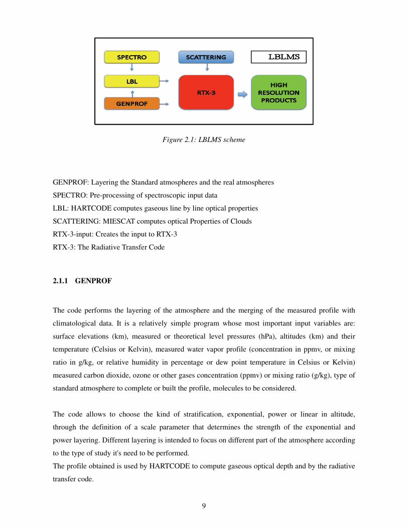
Figure 2.1 shows a simple scheme of the codes chain.
9
Figure 2.1: LBLMS scheme
GENPROF: Layering the Standard atmospheres and the real atmospheres
SPECTRO: Pre-processing of spectroscopic input data
LBL: HARTCODE computes gaseous line by line optical properties
SCATTERING: MIESCAT computes optical Properties of Clouds
RTX-3-input: Creates the input to RTX-3
RTX-3: The Radiative Transfer Code
2.1.1 GENPROF
The code performs the layering of the atmosphere and the merging of the measured profile with
climatological data. It is a relatively simple program whose most important input variables are:
surface elevations (km), measured or theoretical level pressures (hPa), altitudes (km) and their
temperature (Celsius or Kelvin), measured water vapor profile (concentration in ppmv, or mixing
ratio in g/kg, or relative humidity in percentage or dew point temperature in Celsius or Kelvin)
measured carbon dioxide, ozone or other gases concentration (ppmv) or mixing ratio (g/kg), type of
standard atmosphere to complete or built the profile, molecules to be considered.
The code allows to choose the kind of stratification, exponential, power or linear in altitude,
through the definition of a scale parameter that determines the strength of the exponential and
power layering. Different layering is intended to focus on different part of the atmosphere according
to the type of study it's need to be performed.
The profile obtained is used by HARTCODE to compute gaseous optical depth and by the radiative
transfer code.

10
2.1.2 SPECTRO & HARTCODE
HITRAN spectroscopic data need to be pre-processed to be used in the computation of the
atmospheric optical depths. A first version of the pre-processing software package SPECTRO, was
set up in 1997 [Miskolczi and Rizzi, 1997]. A new version has been recently developed (2002) by F.
Miskolczi , at that time affiliated with NASA, Langley, VA, USA. Database pre-processed is the
HITRAN 2000.
The SPECTRO tasks, in this chain of codes, is to filter out some transitions, select the required lines
depending on the specified molecules and slant path from the HITRAN database and pre-process
the spectroscopic data with line mixing. Line mixing is a term to describe the effect of the pressure
on the closely packed absorption lines belonging to the same vibrational band. Whenever the line
spacing is comparable to the pressure broadened half-width, the lines begin to overlap and
collisions will broaden and mix the lines creating interference terms in the band shape and the band
shape will narrow with the increasing pressure. According to results of the validations of the LbL
codes, ignoring the CO2 Q-band line mixing could be responsible for errors of about 20% in the
computed outgoing long-wave spectral radiance [Miskolczi and Rizzi, 1997].
The pre-processed spectroscopy data is the input to the HARTCODE code.
The High-resolution Atmospheric Radiance Transmittance CODE (HARTCODE) was developed
under the support of the International Centre for Theoretical Physics, Trieste, Italy [Miskolczi et al.,
1988a], [Miskolczi et al., 1988b], [Miskolczi et al.,1990]. Within the LBLMS suite HARTCODE
has been used to generate the high resolution optical depths from the observer's altitude (generally
the top of the atmosphere) to the various levels. This product is later used by another code (RTX3-
Input) to compute layers' optical depths.
In HARTCODE the wave number domain is divided into steps. The computation passes throughout
the wave-number domain from a starting wave number to an ending wave number in previously
defined steps. The length of a step is optional, and usually limited by the computer's capability.
Typically, in infrared region steps can have values of 0.5, 1.0 and 2 cm-1 and output blocks of the
required spectral quantity will be generated at each step.
The steps are further divided into smaller sub-intervals, (SI), which represent the resolution of the
computation. The output blocks of each step will contain the integrated (or averaged) spectral
optical depth, transmittance and radiance over each SI. The length of a sub-interval is limited only
by a parameter statement of the code, and typical length settings for 1 cm-1 steps normally range
from 0.001 to 1.0 cm-1. Depending on the positions of all the lines falling within SI, a fine mesh
11
structure is created. In this fine mesh structure, each line center is represented with one point, and
starting from each line center several additional points are added. The positions of the additional
points are depending on the minimal Voigt half-width along the whole trajectory, and on an input
scaling factor (IANT). The scaling factor controls the number of mesh points to be added within
one half-width from the line center. Getting farther from the line center this number will decrease
according to a power function. The above mesh structure defines the sub-sub-intervals (SSI) over
which variable order Gaussian quadrature is applied to perform the wave number integration. The
accuracy of the wave number integration over SI will depend on the number of SSI and on the order
of Gaussian quadrature used in each SSI.
The lines between the end-points of a step and the beginning of the two side intervals are treated
similarly to the lines within the step. They are always contributing to the monochromatic optical
depth using the proper Voigt line shape.
In the recent version of HARTCODE the contribution from the lines being further than the extent of
the outer side-intervals are not considered. This contribution is generally referred as far-wing
absorption. Accurate far-wing absorption can only be computed from accurate line shape functions.
Far from the line centers the shapes of the absorption lines are, however, not sufficiently well
known, and significant error may be introduced into the related absorption term. Whenever
experimental results prove with sufficient accuracy that a particular molecule has continuum type
absorption, then the best strategy is to consider this absorption by a parameterized wave-number
dependent database.
The water vapor continuum adopted is the CKD version 2.4 [Clough et al., 1980], [Clough et al.,
1989]. Finally the pressure-broadened band of N2 at 2350 cm-1 [Menoux et al., 1993] and that of
O2 at 1550 cm-1 [Timofeyev and Tonkov, 1978], [Rinsland et al., 1989] are also included as
broadband continuum contributions to the absorption.
The integrated quantities over the SI intervals (optical depth or trasmittance) can be computed from
the monochromatic optical depth and transmittance values.
The best method would be to compute average transmittances (to be used in RTX-3) from a
reference level (say top of the atmosphere=TOA) to each level in the atmosphere. The ratio of these
average transmittances in two successive levels is in fact the most accurate value for the layer
average transmittance that can be obtained, but only for the down-looking geometry. The problem
with this procedure is that it is easy to reach a value of zero for the average transmittance and from
that point down (or up) it is not possible to reconstruct the layer optical depth.
An alternate method is to integrate the optical depths in each sub-interval to obtain the average
optical depth. The difference of optical depth in two successive levels is another estimate of the
layer optical depth. The problem with this procedure is that the average layer optical depth is a
12
poor representation, because it generates layers which are too opaque, of the average transmittance
for the layer when there are large variations in optical depth within the sub-interval SI.
A third method relies on the computation of the average transmittance in each layer, not the one
integrated from a reference level (say TOA) to each level down. The problem is that, although the
total monochromatic transmittance from TOA to a certain level can be accurately computed by
multiplying the layer monochromatic transmittances, this is not true for the average layer
transmittances. In principle therefore the third method is inferior to the first method, but does not
have the problem of the latter if the atmospheric layers are thin enough so that none has zero
average transmittance. Therefore all three methods have some drawbacks. Although RTX is used to
compute radiance in all directions at all levels, different sets of transmittances or optical depths (for
example, one computed from TOA to each level and the other from surface to each level) can't be
used defining the appropriate effective layer average transmittance separately for upwelling and
downwelling radiances. Instead it has been decided to compute one set of transmittances (or optical
depths) that is most appropriate for the experiment at hand and compute the layer average spectral
optical depth as a property of the layer.
2.1.3 MIESCAT
MIESCAT is used to compute the optical properties of distributions of particles. The code is a
modified version of MIESCAT code by Frank Evans. The only databases requested are the
refractive index of water, ice and eventually aerosols and their weight densities.
Pure liquid water refractive indexes database consist of the laboratories data taken by Segelstein
[1991] in the range 10-3
– 103
cm-1
(10 µm to 10 m)a correction can be applied to account for
temperature dependance based on the Ray's model [1972].
Ice refractive index values are taken from Warren's Tables [1984], that cover the range from 0.045
µm to 8.6 m. The temperature dependence is included for temperatures between 213 and 272 K and
for wavelengths above 167 µm (60 cm-1
).
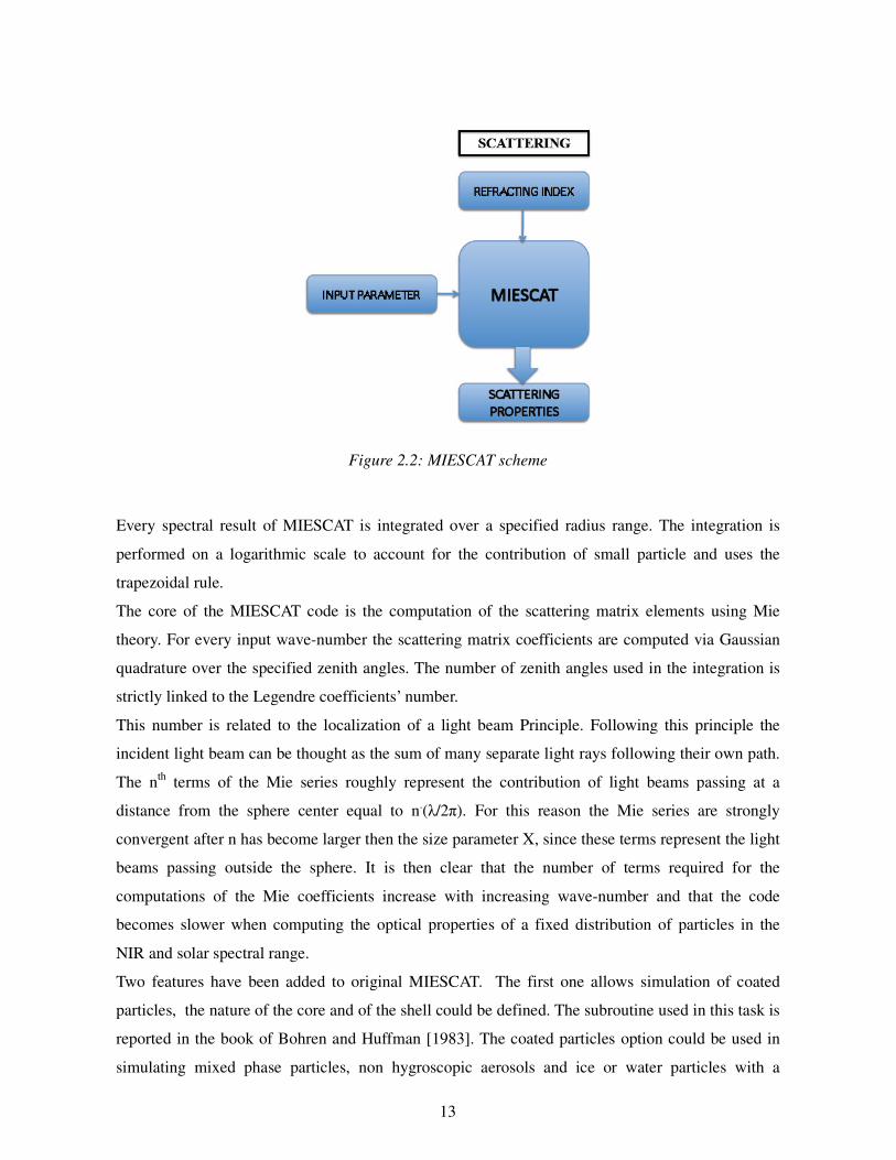
The code, whose simplified input/output structure is shown in Figure 2.2, is very flexible and
adapted to compute the following spectral optical properties over a large spectral interval:
• volume extinction and scattering coefficients [1/km] of a 1 km thick layer of spherical
particles and the single scattering albedo.
• Legendre coefficients for the four independent scattering matrix elements. These coefficients
are in terms of the Stokes vector and are normalized.
13
Figure 2.2: MIESCAT scheme
Every spectral result of MIESCAT is integrated over a specified radius range. The integration is
performed on a logarithmic scale to account for the contribution of small particle and uses the
trapezoidal rule.
The core of the MIESCAT code is the computation of the scattering matrix elements using Mie
theory. For every input wave-number the scattering matrix coefficients are computed via Gaussian
quadrature over the specified zenith angles. The number of zenith angles used in the integration is
strictly linked to the Legendre coefficients’ number.
This number is related to the localization of a light beam Principle. Following this principle the
incident light beam can be thought as the sum of many separate light rays following their own path.
The nth
terms of the Mie series roughly represent the contribution of light beams passing at a
distance from the sphere center equal to n.(λ/2π). For this reason the Mie series are strongly
convergent after n has become larger then the size parameter X, since these terms represent the light
beams passing outside the sphere. It is then clear that the number of terms required for the
computations of the Mie coefficients increase with increasing wave-number and that the code
becomes slower when computing the optical properties of a fixed distribution of particles in the
NIR and solar spectral range.
Two features have been added to original MIESCAT. The first one allows simulation of coated
particles, the nature of the core and of the shell could be defined. The subroutine used in this task is
reported in the book of Bohren and Huffman [1983]. The coated particles option could be used in
simulating mixed phase particles, non hygroscopic aerosols and ice or water particles with a
14
radiatively important cloud condensation nuclei.
The second upgrade concerns the possibility to compute the optical properties of single aerosols
components. This upgrade can be considered as a completion of the previous one when non
hygroscopic aerosols are taken into account and coated particles are formed in the atmosphere.
Particular attention has been given to hygroscopic aerosols since the relative humidity affects the
variables defining the particles size distribution, the value of the particles’ densities and index of
refraction. The mass increase coefficients defined and measured by Hänel [1976] and Hänel and
Lehmann [1981] are used. However present knowledge about the increasing coefficients is very
poor and data for different components are required if an exhaustive study concerning hygroscopic
aerosols has to be performed.
2.1.3.1 PARTICLE SIZE DISTRIBUTIONS
It is common use to indicate with n(r)dr the number of particles in a unit volume with radius r
assuming values between r and r+dr. Analytic functions used to describe the size distribution
generally use four parameters to characterize a size distribution: the radius value of the smaller and
larger particle, defining the radius spectrum over which the distribution is taken, and two additional
parameters related to the peak and spread of the distribution: usually the effective radius and
effective variance.
The MIESCAT code has been adapted to use two different types of size distributions: the Standard
Hansen H71 [Hansen, 1971] and the Lognormal. Even if a climatology of the particles’ size
distributions present in different types of clouds is not yet satisfactory, the H71 seems to yield very
good results when simulating both high and low clouds.
For a very large value of Veff, the maximum number concentration is found at the lower limit of the
distribution. Such characteristic of numerical density distribution is not uncommon and for example
is reported by D. Mitchell [2002] as a typical example of size distribution sampled in anvil cirrus
during CEPEX.
The use of gamma type distributions in simulating ice and water clouds is widely accepted by the
scientific community. Among various examples, in the recent work by A.J. Heymsfield [2003a;
2003b] and A.J. Heymsfield et al. [2003] gamma type distributions are used to fit measured ones
when studying radiative and microphysical properties of Tropical and Mid Latitude ice cloud
ensembles.
The Lognormal distribution is sometimes applied in the representation of cloud droplets size
distributions. In fact, among many other authors, Frisch et al. [2002] noted its computationally
15
convenience, with respect to the modified gamma, and its good approximation of water clouds
distributions when applied to retrieval methods using cloud radars.
2.1.4 RTX-3-input
HARTCODE was intended, since its creation, a ‘stand-alone’ code to compute spectral radiances,
fluxes and cooling rates in clear sky conditions, with the possibility to account for diverse viewing
geometries including limb trajectories, that is it wasn’t thought as to be part of a sequence of codes.
Nowadays, HARTCODE is used for computing the gaseous optical depth from the top of the
atmosphere to the various levels’ altitudes,as explained before.
Some operations have to be performed in order to interface HARTCODE to RTX-3 input structure
and insert some additional and necessary information. This role is played by the code RTX-Input.
First of all RTX-Input converts HARTCODE’s output optical depths from the TOA to each level to
optical depths of each layer (defined by two adjacent levels). Moreover it writes the top of the
atmosphere solar irradiances, interpolated at the same spectral resolution defined for the gas optical
depths computation. The solar irradiance database consists of “solar constant” values in the interval
from 0 to 50000 cm-1
[Kurucz, 1997] tabulated every 1 cm-1
.
The inter-annual variability is computed following orbital data accounting for the elliptical shape of
the earth’s orbit. The corrections applied can reach the 3% of the sun irradiance value at the mean
distance.
A very important point in the execution of RTX-Input is the evaluation of the surface spectral
reflectivity (r). The surface is assumed as non-transmittive (t = 0), so that for every wave-number
holds the following relation:
1 = r + e ,
where e is the spectral emissivity.
At the moment, an emissivity database for different types of land surfaces is not available, so when
simulating the radiative transfer over land surfaces a standard value of 1 is set for e.
Ocean surface emissivity is computed using a program called COMP_EMISSIVITY, developed by
Matricardi in 1999 and later modified by various members of the ADGB group. The computation
follows the methods explained in Masuda et al. [1988] and takes into account wind speed and
viewing angle. The number of points for the Masuda integration is 100 for angles below 60° and
16
200 for angles equal or greater than 60°. The index of refraction of ocean water used in the
COMP_EMISSIVITY model, is obtained from:
Wieliczka et al. [1989], corrected for sea water by Friedman [1969] for wave-numbers between 500
and 8117 cm-1
(to note that correction for salted water are very small with respect to pure water),
Segelstein [1981] without marine correction for wave-numbers between 0.001 and 500 cm-1
and
between 8117 and 106 cm
-1.
A wide database for different viewing angles and wind speeds has been created and made accessible
to RTX-Input. Since the spectral emissivity has been computed for specified wave-numbers an
interpolation is required in RTX-Input.
2.1.5 RTX-3
The code RTX-3 is used to solve the radiative transfer equation in a multiple scattering
environment.
RTX-3 solves the plane parallel case of polarized monochromatic radiative transfer for isotropic
media by the use of the adding and doubling method, due to Van de Hulst and described by various
authors among which Goody and Yung [1989] and Liou [1992]. The original version of the model
(RT3) was developed by Evans and Stephens [1991]. The same authors modified the original
algorithm to allow the output of radiances at any level in the input layer file and added an option to
perform a Delta-M scaling (1995-96). The code has been adapted to allow sequential computation
at different wave-numbers.
The layers are assumed uniform and infinite in horizontal extent and may be of any thickness. The
geometrical properties of the layers are given by the GENPROF output.
The radiation field may have full angular dependence (zenith and azimuth angles). The angular
variation of radiance is expressed as a Fourier series in azimuth and by discretization in a number of
zenith angles. For every wave-number the calculations are performed sequentially for each azimuth
mode.
The key concept behind the doubling and adding method is the Interaction Principle, which
expresses the linear interaction of radiation with a medium: radiation emerging from a layer is
related to radiation incident upon the layer and to radiation generated within the layer. For each
layer, computing the reflection matrix R, the transmission matrix T, and the source vector S,
amounts to solve the radiative transfer equation. The transformation of the single scattering
information (coefficients of the Legendre series in the scattering angle) into a form suitable for the
17
radiative transfer model is performed first: that means to perform a polarization transformation from
the phase matrix P to the scattering matrix M. A clear explanation of the methodology used can be
found in the reference text of Evans and Stephens [1991]. From the initial infinitesimal sub-layer,
the doubling method builds up the radiative properties of the finite homogeneous layer performing a
number of steps depending on the sub-layers thickness. An extension of the doubling method,
developed by Wiscombe [1976], to incorporate sources that vary exponentially with optical depth is
considered. Within each layer, in fact, the source function is linear in optical depth for the thermal
case and exponential in optical depth for the solar case.
If the layer doesn't scatter the reflection and transmission matrices and source vector are calculated
rather than using initialization and doubling.
For each output level an adding method is introduced to combine the layers above and below the
output level. Then the radiance at the output level from the reflection and transmission matrices and
source vectors for the medium above and below and the radiance incident from the boundaries are
evaluated. The sources of radiation are the solar direct beam and thermal emission. There is
assumed to be thermal and/or reflected direct solar radiance from the lower surface. The ground
surface can be Lambertian (isotropic emissivity) or follows the Fresnel’s reflection formulae. Until
now only the Lambertian surface may be used with a solar source.
The number of Gaussian quadrature points and Legendre coefficients are related. A limit on the
maximum number of Legendre terms is enforced by truncating the series at the appropriate degree.
An analysis of the effects of truncation of the Legendre series on simulated brightness temperature
at the top of the atmosphere is given in Loffredo [2000].
18
2.2 MICROWAVE REMOTE SENSING
2.2.1 Gaseous line by line optical properties
The principal sources of atmospheric microwave emission and absorption are water vapor, oxygen,
and cloud liquid. In the frequency region from 20 to 200 GHz, water-vapor absorption arises from
the weak electric dipole rotational transition at 22.235 GHz and the much stronger transition at
183.31 GHz. In addition, the so-called continuum absorption of water vapor arises from the far
wing contributions from higher-frequency resonances that extend into the infrared region. Again, in
the frequency band from 20 to 200 GHz, oxygen absorbs due to a series of magnetic dipole
transitions centered around 60 GHz and the isolated line at 118.75 GHz. Because of pressure
broadening, i.e., the effect of molecular collisions on radiative transitions, both water vapor and
oxygen absorption extend outside of the immediate frequency region of their resonant lines. There
are also resonances by ozone that are important for stratospheric sounding [Gasiewski, 1993]. In
addition to gaseous absorption, scattering, absorption, and emission also originate from
hydrometeors in the atmosphere.
In general, the absorption coefficient ka at frequency f due to a particular gas can be written in the
form
( ) ( ) _a i ik f = N S F f +continuum terms∑ (2.1)
Where Si is the intensity (dependent of temperature) of line i, Fi(f) is the shape factor for line i and
N is the abundance of the gas, corresponding to the definition of line intensity. In the HITRAN and
GEISA databases, for example, the definition of line intensity requires N to be the molecule number
density of the absorption gas (i.e. relative isotopic abundance is contained in Si); but this definition
is not universally followed in the literature. The selection of lines to be included in the summation
of Eqn. (2.1) may require the exercise of some educated judgment on the part of the user who
wishes to compare calculations with a particular set of measurements. The total absorption by a
mixture of gases is the sum of absorption coefficients from the individual species under the
conditions of pressure, temperature and abundances existing in the mixture. One may combine
absorption model for different gases from different sources; hence, the number of possible
combination is large [Mätzler, 2006].
19
2.2.2 Water Vapour Absorption and continuum
Hill [1986] devised a test criterion that responds to line shape while being insensitive to width or
continuum level. He applied this test to the water vapour absorption data of Becker and Autler
[1946] near 22 GHz and found that the Van Vleck-Weisskopf line shape was an acceptable fit to that
line, while the Gross and full Lorentz line shapes where rejected.
The line shape factor of Van Vleck and Weisskopf is
( )( )( ) ( )( )
2
2 22 2
1 i ii
i i i i i i i
w wfF f
f f f w f f wπ δ δ
= + − − + + + +
(2.2)
In the above, fi is the line frequency, δi is the line shift and wi is the half-line width; wi and δi depend
on temperature.
The expression
( )( )( )
2
2 2
1 ii
i i i i
wfF f
f f f wπ δ
= − − +
(2.3)
is the Lorentz shape of structure-factor commonly given in the literature, and is a good
approximation when wi and |f - fi - δi | are both small in magnitude compared with f. These
conditions are well fulfilled when one deals with the absorption of visible or infra-red light. In
studying the absorption at low microwaves frequencies, which fall outside sharp resonances, these
conditions may not be respected and it's necessary to use the more exact formula, Eqn. (2.2).
As shown in Eqn. (2.1) models for atmospheric water vapor transmittance include an empirical
component which is called the "continuum", in addition to line contributions.
The water vapor continuum contributes most of the opacity of a clear midlatitude or tropical
atmosphere at window frequencies of 30 GHz or higher.
Several possible causes of the H2O continuum have been proposed, among them (1) the inadequacy
of analytic line shapes at frequency displacements of hundreds of GHz from the centers of the
extremely strong far-infrared lines, (2) a possible spectral contribution from water dimers, clusters
of molecules or weakly bound complexes, (3) collision-induced absorption and (4) co-operative
absorption pairs of molecules.
Practically hypothesis n. 1) above is considered the most probable and the continuum is empirically
20
modeled as the difference between observed absorption and what can be described by conventional
line profiles, such as the Van Vleck-Weisskopf's.
Laboratory measurements of water vapor's microwave-window absorption have been made by
Frenkel and Woods [1966], Liebe [1984], Liebe and Layton [1987], Godon et al. [1992], and Bauer
et al. [1993, 1995, 1996]. There is a consensus that the continuum has two components: one
proportional to the square of water vapor partial pressure, the other proportional to the product of
water vapor and foreign gas partial pressures. The first component has a much stronger dependence
on temperature than the second. These characteristics indicate that the first component originates in
interactions between two water molecules, at distances close enough that the deep potential well
formed by these polar molecules is important, while the second component is due to binary
interactions involving a water molecule and a foreign-gas molecule.
A large body of experimental work and associated modelling has been recently produced;
Rosenkranz [1998] has reviewed most of these models suggesting a resolution of some of the
discrepancies, and recommending a model for atmospheric radiance transfer calculation. The
Rosenkranz model will be briefly presented in Paragraph 2.3.
2.2.3 Oxygen absorption
Oxygen is unusual in that it absorbs microwaves by means of a magnetic dipole moment than an
electric dipole moment. Consequently, the molecules exhibit both resonant and non-resonant
absorption in the gas phase. For O2, pressure line shift appears to be negligible, but calculation of
the absorption requires the addition to equation (2.2) of first order line mixing (sometimes called
line-coupling) parameters Yi, which are also dependent on temperature and proportional to pressure:
( )( )( )
( )( )( )( )
( )( )
2
2 22 2
1 i i i i i i
i
i i i i i
w f f Y w f f YfF f
f f f w f f wπ
+ − − − = + − + + +
(2.7)
Because the Yi in Eqn. (2.7) arise through the mixing of lines due to correlation of the molecular
state before and after collisions, they have physical meaning only in a summation over lines, such
as in Eqn. (2.1). Correct calculation of the line-mixing effect requires the summation to include all
of the terms considered in derivation of the mixing coefficients, including the non-resonant term. It
is also necessary to realize that the mixing parameters and widths are associated; thus they should
not be obtained from different sources. On the wings of the O2 band, the net effect of line mixing is
21
to reduce absorption, as though molecular collisions were less effective at broadening the lines.
2.2.4 Nitrogen absorption
Nitrogen has no microwave lines, but it does exhibit a weak continuum absorption due to collision-
induced dipole moments, as do other molecules, including oxygen.
2.2.5 Particles Optical Properties
For spherical particles, the classical method to calculate scattering and absorption coefficients is
through the Lorenz-Mie Equations [Mattioli et al., 2005; Van de Hulst, 1981; Deirmendjian ,1969];
for sufficiently small particles, the Rayleigh approximation can be used. For a given wavelength
and single particle, the particle contribution is calculated; the total coefficients are then obtained by
integration over the size distribution of particles. An important physical property for the
calculations is the complex dielectric constant of the particle. This dielectric constant of liquid
water is described by the dielectric relaxation spectra of Debye [1929]. The strong temperature
dependence of the relaxation frequency is linked to the temperature-dependent viscosity of liquid
water; therefore the cloud-absorption coefficient also shows significant temperature sensitivity.
22
2.3 TBARRAY AND TBSCAT
TBARRAY is a code which computes microwave emission and transmission for an atmospheric
profile at multiple angles at the top of atmosphere or at surface in the range between 0 to 1000 Ghz.
It evaluates absorption by the atmospheric gases oxygen, water vapor and nitrogen as well as by the
cloud liquid water, considering scattering negligible.
TBSCAT computes top-of-atmosphere microwave brightness temperatures for a multiple scattering
atmosphere defined by profiles of temperature, water-vapor density, (non-precipitating) cloud liquid
water density and density profiles of up to four types of precipitation (rain, snow, graupel, and ice),
all specified as functions of pressure.
Planar stratification of the atmosphere is assumed, which implies azimuthal symmetry of emitted
brightness temperature.
TBSCAT includes absorption by oxygen, water vapor and nitrogen and by cloud liquid water and
computes Mie scattering and extinction for spherical particles. The equation of radiative transfer is
solved by the method of Rosenkranz [2002,2007].
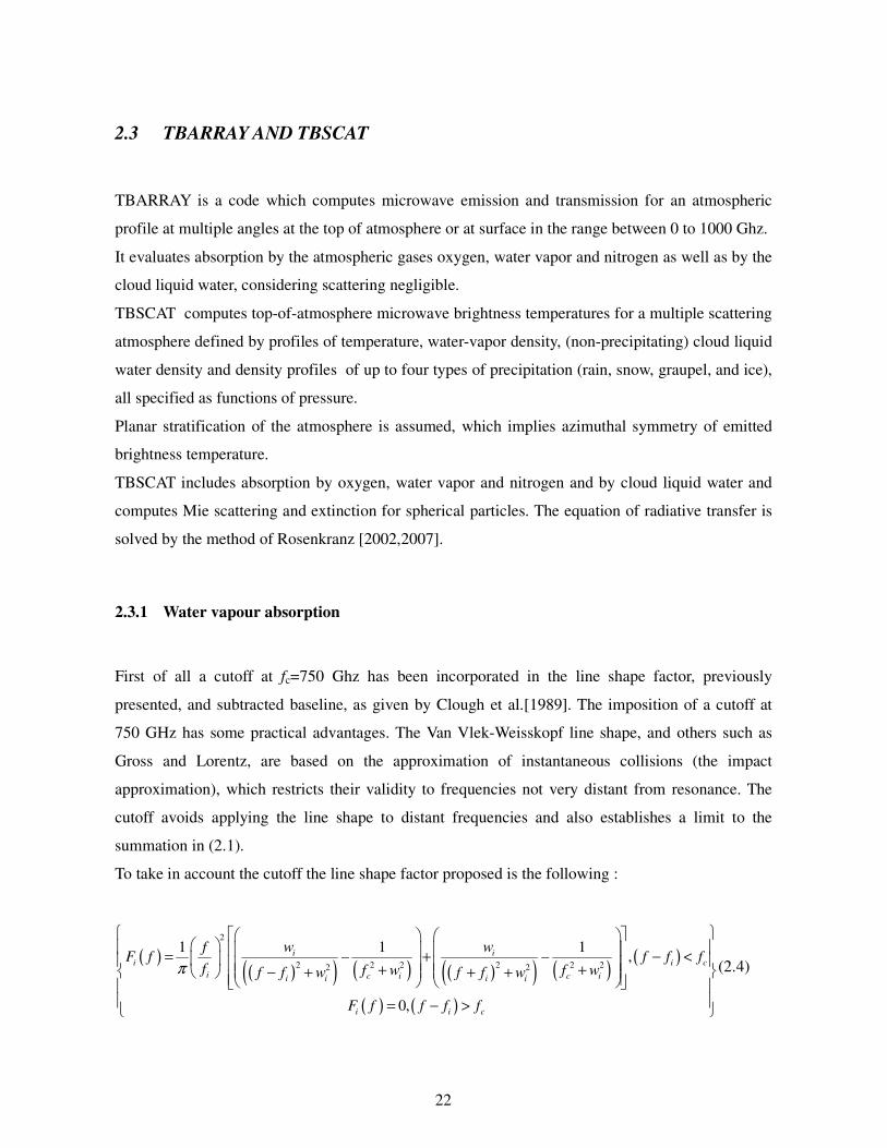
2.3.1 Water vapour absorption
First of all a cutoff at fc=750 Ghz has been incorporated in the line shape factor, previously
presented, and subtracted baseline, as given by Clough et al.[1989]. The imposition of a cutoff at
750 GHz has some practical advantages. The Van Vlek-Weisskopf line shape, and others such as
Gross and Lorentz, are based on the approximation of instantaneous collisions (the impact
approximation), which restricts their validity to frequencies not very distant from resonance. The
cutoff avoids applying the line shape to distant frequencies and also establishes a limit to the
summation in (2.1).
To take in account the cutoff the line shape factor proposed is the following :
( )( )( ) ( ) ( )( ) ( )
( )
( ) ( )
2
2 22 2 2 22 2
1 1 1– – ,
0,
i ii i c
i c i c ii i i i
i i c
w wfF f f f f
f f w f wf f w f f w
F f f f f
π
= + − < + +− + + +
= − >
(2.4)
23
The half width wi is calculated as
( )( ) ( )
2
xx fsi s f f
Hw = w P θ + w P θ
O (2.5)
where ws , xs , wf and xf are constant coefficient, θ is 300/T with T in Kelvins accounting for the
effect of the departure of temperature from the 300-K value, PH2O is the partial pressure of water
vapour, and Pf is the partial pressure of dry air.
The equation proposed for the continuum is due to a combination of the foreign-broadening
continuum from MPM87 (Millimeter-wave Propagation Model) [Liebe et Layton, 1987] and the
self-broadened continuum from MPM93 [Liebe et al, 1993] with the necessary adjustments to be
compatible with the use of a cutoff line shape, and is
( ) ( )3
2 2
22
f f sH H
CONTINUUM = f θ C P P +C PO O
(2.6)
where Cf and Cs are coefficients that depend on temperature and frequency and include the
adjustment to compensate for the use of Eqn. (2.4) instead of a pure VanVleck-Weisskopf line shape
[Rosenkranz, 1998].
2.3.2 Scattering
In TBSCAT, the Mie theory is applied using the parameterization proposed by Diermendjian [1969]
with a Rayleigh limit applied following Wiscombe [1976].
Water and pure Ice complex dielectric constant are evaluated, as in the cloud liquid water case, with
the formulas proposed by Liebe and Hufford [1991]. An interesting feature of the model is the
opportunity to reproduce an approximate electromagnetic description of snow, groupel or pure ice
introducing the concept of the ice-factor F(λ), which is a fractional volume of ice in an air matrix,
based on Sihvola's [Sihvola, 1989; Karkainen et al.,2001] dielectric mixing theories.
Snow and graupel are in fact heterogeneous materials composed of ice and air. Since the density of
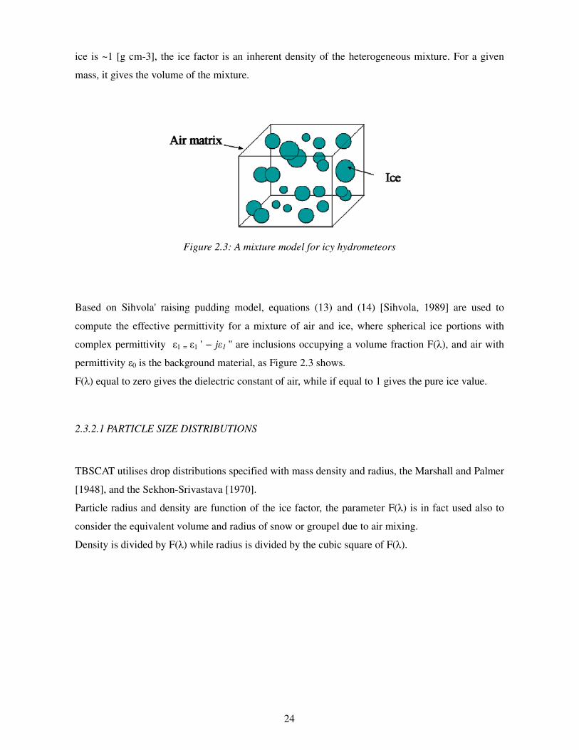
24
ice is ~1 [g cm-3], the ice factor is an inherent density of the heterogeneous mixture. For a given
mass, it gives the volume of the mixture.
Figure 2.3: A mixture model for icy hydrometeors
Based on Sihvola' raising pudding model, equations (13) and (14) [Sihvola, 1989] are used to
compute the effective permittivity for a mixture of air and ice, where spherical ice portions with
complex permittivity ε1 = ε1 ' − jε1 '' are inclusions occupying a volume fraction F(λ), and air with
permittivity ε0 is the background material, as Figure 2.3 shows.
F(λ) equal to zero gives the dielectric constant of air, while if equal to 1 gives the pure ice value.
2.3.2.1 PARTICLE SIZE DISTRIBUTIONS
TBSCAT utilises drop distributions specified with mass density and radius, the Marshall and Palmer
[1948], and the Sekhon-Srivastava [1970].
Particle radius and density are function of the ice factor, the parameter F(λ) is in fact used also to
consider the equivalent volume and radius of snow or groupel due to air mixing.
Density is divided by F(λ) while radius is divided by the cubic square of F(λ).
25
2.4 LBLMS IMPLEMENTATIONS
Rosenkranz's models analyses and the theory presented have been used as test beds to implement
the extension of the ADGB model to the microwave region.
The first analysis proposed is about the gaseous optical properties.
2.4.1 Gaseous line by line optical properties
The codes SPECTRO and HARTCODE, and TBARRAY have been used to simulate the optical
properties of two of the six standard atmospheres [Anderson, 1986], and a first comparison has been
proposed between the two models.
The tropical standard atmosphere (TRO) has the highest tropospheric thermal gradient and a
particularly thin Tropopause (set at about 16 km). On the opposite, the Sub Arctic Winter
atmosphere (SAW) has the Tropopause starting at only 9 km and it maintains an almost isothermal
or very slowly decreasing temperature profile till 25 km. The latter atmosphere is also very
interesting for its thermal inversion from the ground to 1.125 km, a consequence of the extremely
low surface temperatures reached at high latitudes in the winter season. The two mentioned
atmospheric profiles correspond to extreme situations.
To better understand the differences due to gaseous contribution a simplified surface with a constant
unit emissivity has been used.
Upwelling brightness temperatures obtained with the two models are proposed in Figure 2.4 and
2.5.
26
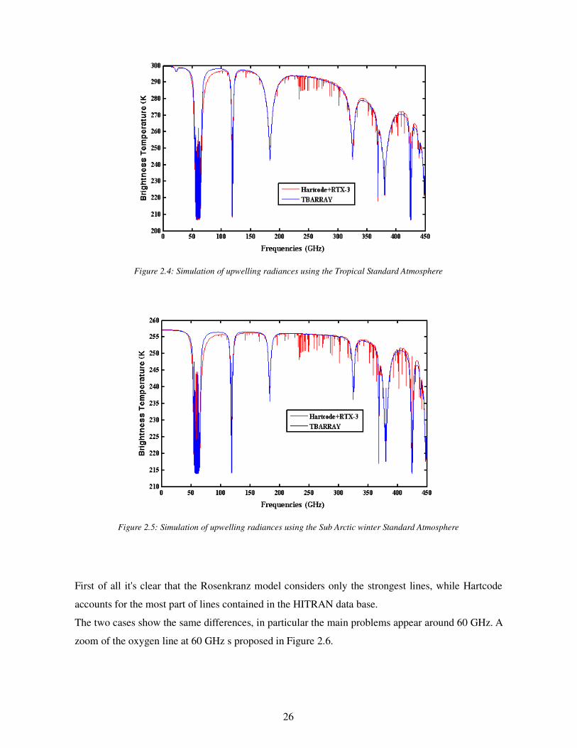
Figure 2.4: Simulation of upwelling radiances using the Tropical Standard Atmosphere
Figure 2.5: Simulation of upwelling radiances using the Sub Arctic winter Standard Atmosphere
First of all it's clear that the Rosenkranz model considers only the strongest lines, while Hartcode
accounts for the most part of lines contained in the HITRAN data base.
The two cases show the same differences, in particular the main problems appear around 60 GHz. A
zoom of the oxygen line at 60 GHz s proposed in Figure 2.6.
27
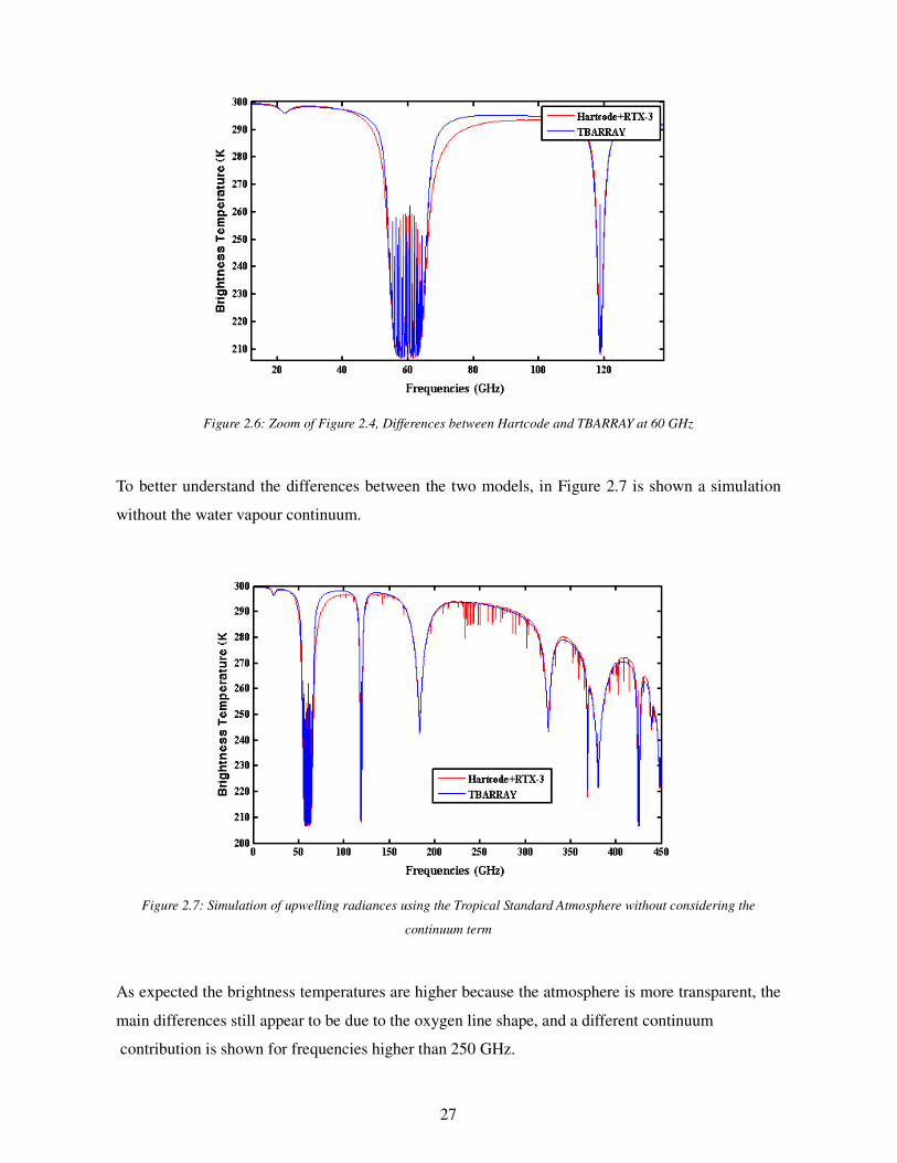
Figure 2.6: Zoom of Figure 2.4, Differences between Hartcode and TBARRAY at 60 GHz
To better understand the differences between the two models, in Figure 2.7 is shown a simulation
without the water vapour continuum.
Figure 2.7: Simulation of upwelling radiances using the Tropical Standard Atmosphere without considering the
continuum term
As expected the brightness temperatures are higher because the atmosphere is more transparent, the
main differences still appear to be due to the oxygen line shape, and a different continuum
contribution is shown for frequencies higher than 250 GHz.
28
The former approach consisted in introducing the oxygen line coupling and the corrections for the
continuum in HARTCODE, but in order to implement a unique code from microwave to visible
region the best option appeared to substitute the SPECTRO – HARTCODE code with a different
model: LBLRTM.
LBLRTM is an accurate line-by-line radiative transfer code developed at the Atmospheric and
Environmental Inc. (AER). It can solve the clear sky radiative transfer equation or it can be used to
obtain layers monochromatic optical depths. A schematic description of the main features of the
code can be found at http://rtweb.aer.com/lblrtm_frame.html.
A series of codes have been written to create LbLRTM files (Tapes).
LbLRTM spectroscopic input parameters are obtained by running the LNFL program
[http://rtweb.aer.com/main.html] with a line file database for the spectral lines and cross sections for
the heavy molecules. The spectroscopic database used is HITRAN 2004. Absorption lines from 38
gases are accounted for from 0.000001 to 25232.0041 cm-1.
Five different continua absorption are also considered in LbLRTM: H2O (MT-CKD 1.3), CO2, N2,
O2 (Herzberg absorption included), O3 (Chappuis/Wulf and Hartley Huggins absorption).
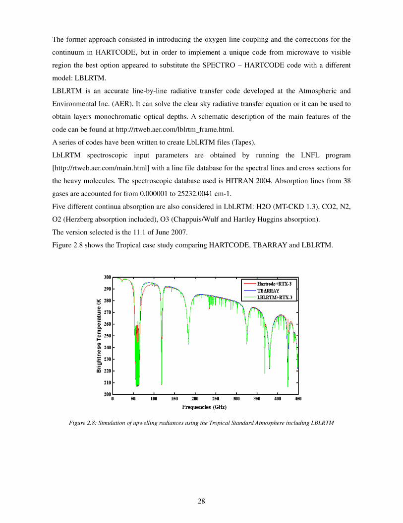
The version selected is the 11.1 of June 2007.
Figure 2.8 shows the Tropical case study comparing HARTCODE, TBARRAY and LBLRTM.
Figure 2.8: Simulation of upwelling radiances using the Tropical Standard Atmosphere including LBLRTM
29
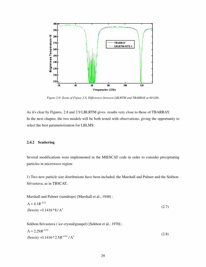
Figure 2.9: Zoom of Figure 2.8, Differences between LBLRTM and TBARRAY at 60 GHz
As it's clear by Figures. 2.8 and 2.9 LBLRTM gives results very close to those of TBARRAY.
In the next chapter, the two models will be both tested with observations, giving the opportunity to
select the best parameterization for LBLMS.
2.4.2 Scattering
Several modifications were implemented in the MIESCAT code in order to consider precipitating
particles in microwave region:
1) Two new particle size distributions have been included, the Marshall and Palmer and the Sekhon-
Srivastava, as in TBSCAT:.
Marshall and Palmer (raindrops) [Marshall et al., 1948] :
0.21
4
4.1
3.1416*8 /
R
Density
−Λ =
= Λ (2.7)
Sekhon-Srivastava ( ice crystal/graupel) [Sekhon et al., 1970].:
0.45
0.94 4
2.29
3.1416*2.5 /
R
Density R
−
−
Λ =
= Λ (2.8)
30
2) Water and pure Ice complex dielectric constant are evaluated, as in TBSCAT, with the formulas
proposed by Liebe and Hufford [1991] in the range between 0 and 1000 GHz, introducing the ice
factor previously presented in Paragraph 2.3.2.
As presented in Paragraph 2.1.3, a model to evaluate water and ice refracting index in microwave
regions was already implemented in MIESCAT, and the new method has been introduced as an
option of the code since both models are frequently used in the literature.
3)-The raising-pudding model of Sihvola has been implemented in MIESCAT to better model snow
and graupel behavior.
2.5 DISCUSSION
The infrared radiative transfer model of the Atmospheric Dynamic Group Bologna has been
modified to work also in microwave region.
To guarantee a correct gaseous optical properties calculation from microwave to the visible region,
LbLRTM has been introduced in place of the SPECTRO&HARTCODE code.
MIESCAT has been modified to evaluate the single scattering properties of precipitating particles,
introducing a new method to evaluate pure water and ice refractive indexes.
Graupel and snowflakes are also modeled introducing the raising-pudding model, and an ice factor
to properly consider the air-ice mixing.
The last part of the code hasn't be changed, the adding-dubbing method is used and gives correct
results in comparison with well known microwave RTM.
The next chapter will present case studies to test the efficiency of the new code.
31
3 APPLICATION OF THE NEW LBLMS TO THE CASE
STUDIES
A data set composed by ground based observations at the North Slope of Alaska site, and space-
borne observations will be simulated with the new version of LBLMS (Chapter2), in order to test
the model performance in clear and cloudy condition, and to evaluate the role of surface and
atmospheric contribution in the Arctic region.
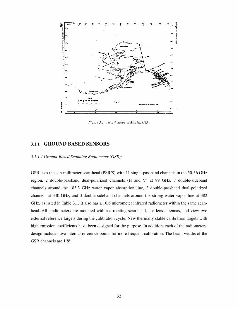
3.1 DATA SET PRESENTATION
An Intensive Operating Period (IOP) was conducted at the U.S. Department of Energy's
Atmospheric Radiation Measurement (ARM) Program's field site near Barrow (North slope of
Alaska, Figure 3.1), Alaska, from March 9th to April 9th 2004. The North Slope of Alaska (NSA) is
the region of the U.S. state of Alaska located on the northern slope of the Brooks Range along the
coast of two marginal seas of the Arctic Ocean, the Chukchi Sea being on the western side of Point
Barrow, and the Beaufort Sea on the eastern. The NSA site has become a focal point for
atmospheric and ecological research activity in the Artcic region, providing measurements in very
dry conditions. several instruments are displayed at this site, the present work will focus on the
Ground-based Scanning Radiometer (GSR), of NOAA's Environmental Technology Laboratory,
and the Microwave Radiometer Profiler (MWRP) of the Atmospheric Radiation Measurement
(ARM) Program that were operational during the IOP.
Three different humidity sensors were deployed from three separate locations near Barrow: ARM
Operational Balloon Borne Sounding System (BBSS) radiosondes were launched daily at 2300
UTC [2 P.M. Alaska standard time (AKST)] at the Great White ARM site (GW). In addition, at the
ARM Duplex (DPLX) in Barrow, 2.4 km to the west of GW, BBSS radiosondes were launched 4
times daily (0500, 1100, 1700, and 2300 UTC). Data from synoptic radiosondes from the National
Weather Service (NWS) (1100 and 2300 UTC) were also archived. The NWS site is in Barrow, 4.9
km to the southwest of GW.
32
Figure 3.1: : North Slope of Alaska, USA.
3.1.1 GROUND BASED SENSORS
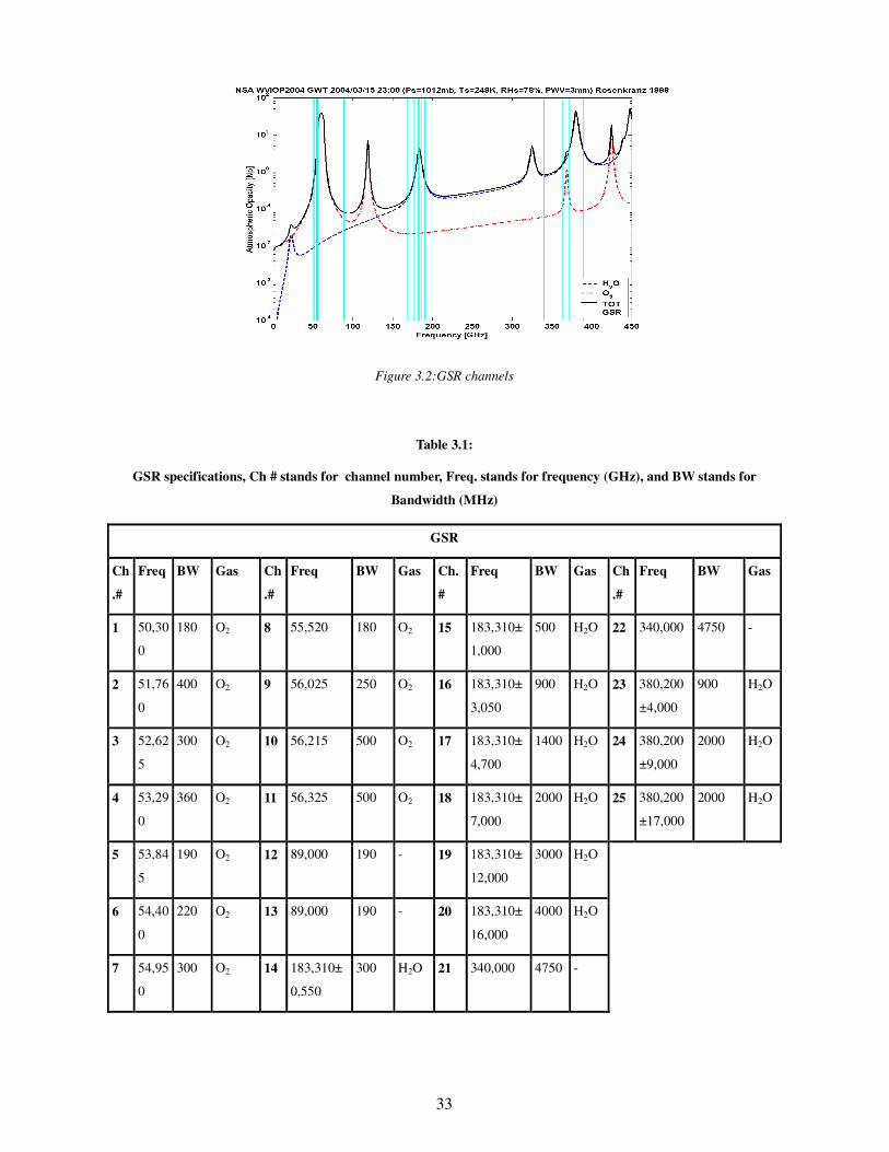
3.1.1.1 Ground-Based Scanning Radiometer (GSR):
GSR uses the sub-millimeter scan-head (PSR/S) with 11 single-passband channels in the 50-56 GHz
region, 2 double-passband dual-polarized channels (H and V) at 89 GHz, 7 double-sideband
channels around the 183.3 GHz water vapor absorption line, 2 double-passband dual-polarized
channels at 340 GHz, and 3 double-sideband channels around the strong water vapor line at 382
GHz, as listed in Table 3.1. It also has a 10.6 micrometer infrared radiometer within the same scan-
head. All radiometers are mounted within a rotating scan-head, use lens antennas, and view two
external reference targets during the calibration cycle. New thermally stable calibration targets with
high emission coefficients have been designed for the purpose. In addition, each of the radiometers'
design includes two internal reference points for more frequent calibration. The beam widths of the
GSR channels are 1.8°.
33
Figure 3.2:GSR channels
Table 3.1:
GSR specifications, Ch # stands for channel number, Freq. stands for frequency (GHz), and BW stands for
Bandwidth (MHz)
GSR
Ch
.#
Freq BW Gas Ch
.#
Freq BW Gas Ch.
#
Freq BW Gas Ch
.#
Freq BW Gas
1 50,30
0
180 O2 8 55,520 180 O2 15 183,310±
1,000
500 H2O 22 340,000 4750 -
2 51,76
0
400 O2 9 56,025 250 O2 16 183,310±
3,050
900 H2O 23 380,200
±4,000
900 H2O
3 52,62
5
300 O2 10 56,215 500 O2 17 183,310±
4,700
1400 H2O 24 380,200
±9,000
2000 H2O
4 53,29
0
360 O2 11 56,325 500 O2 18 183,310±
7,000
2000 H2O 25 380,200
±17,000
2000 H2O
5 53,84
5
190 O2 12 89,000 190 - 19 183,310±
12,000
3000 H2O
6 54,40
0
220 O2 13 89,000 190 - 20 183,310±
16,000
4000 H2O
7 54,95
0
300 O2 14 183,310±
0,550
300 H2O 21 340,000 4750 -
34
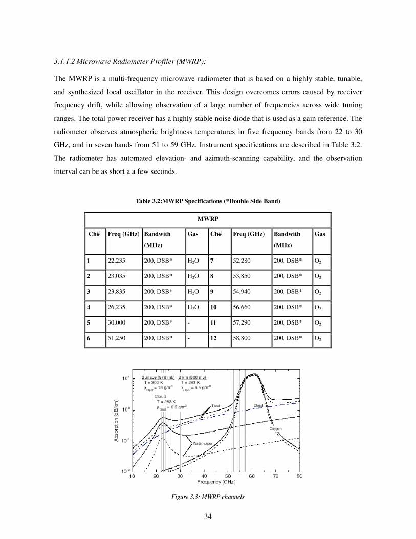
3.1.1.2 Microwave Radiometer Profiler (MWRP):
The MWRP is a multi-frequency microwave radiometer that is based on a highly stable, tunable,
and synthesized local oscillator in the receiver. This design overcomes errors caused by receiver
frequency drift, while allowing observation of a large number of frequencies across wide tuning
ranges. The total power receiver has a highly stable noise diode that is used as a gain reference. The
radiometer observes atmospheric brightness temperatures in five frequency bands from 22 to 30
GHz, and in seven bands from 51 to 59 GHz. Instrument specifications are described in Table 3.2.
The radiometer has automated elevation- and azimuth-scanning capability, and the observation
interval can be as short a a few seconds.
Table 3.2:MWRP Specifications (*Double Side Band)
MWRP
Ch# Freq (GHz) Bandwith
(MHz)
Gas Ch#
Freq (GHz) Bandwith
(MHz)
Gas
1 22,235 200, DSB* H2O 7 52,280 200, DSB* O2
2 23,035 200, DSB* H2O 8 53,850 200, DSB* O2
3 23,835 200, DSB* H2O 9 54,940 200, DSB* O2
4 26,235 200, DSB* H2O 10 56,660 200, DSB* O2
5 30,000 200, DSB* - 11 57,290 200, DSB* O2
6 51,250 200, DSB* - 12 58,800 200, DSB* O2
Figure 3.3: MWRP channels
35
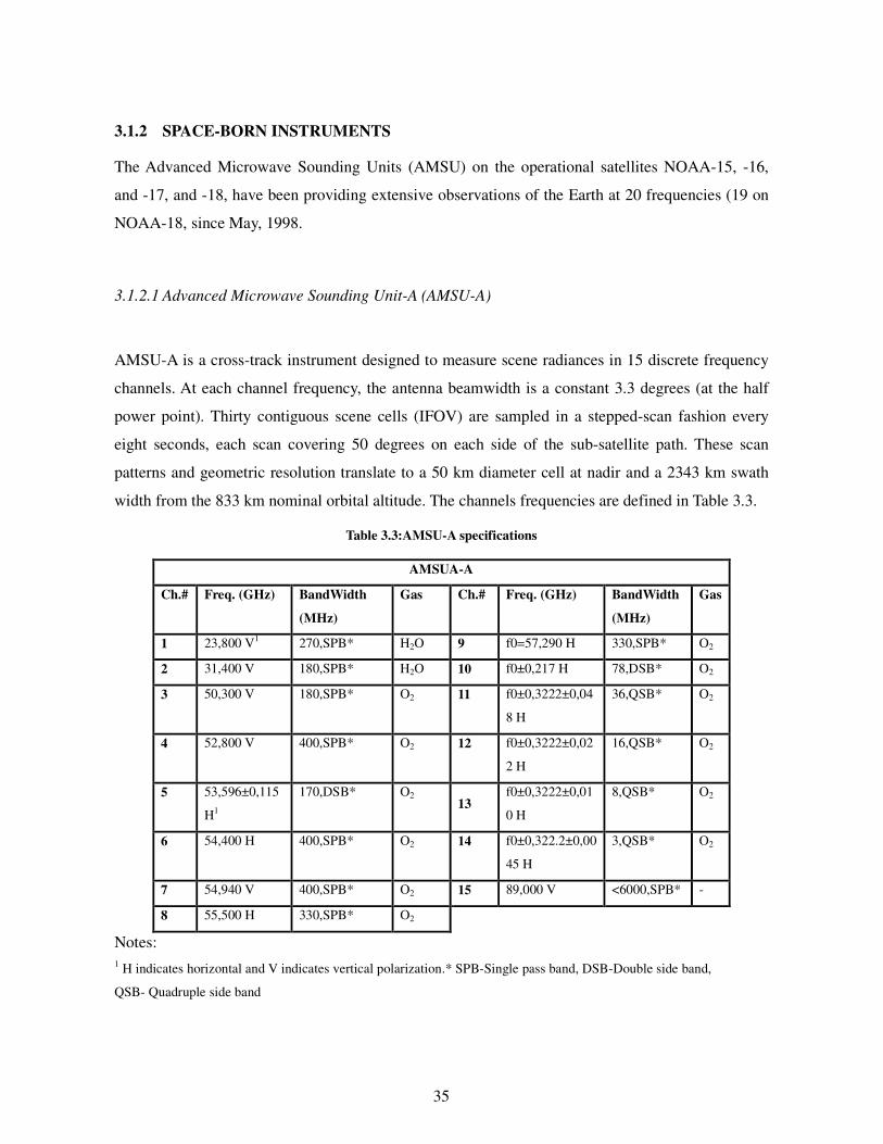
3.1.2 SPACE-BORN INSTRUMENTS
The Advanced Microwave Sounding Units (AMSU) on the operational satellites NOAA-15, -16,
and -17, and -18, have been providing extensive observations of the Earth at 20 frequencies (19 on
NOAA-18, since May, 1998.
3.1.2.1 Advanced Microwave Sounding Unit-A (AMSU-A)
AMSU-A is a cross-track instrument designed to measure scene radiances in 15 discrete frequency
channels. At each channel frequency, the antenna beamwidth is a constant 3.3 degrees (at the half
power point). Thirty contiguous scene cells (IFOV) are sampled in a stepped-scan fashion every
eight seconds, each scan covering 50 degrees on each side of the sub-satellite path. These scan
patterns and geometric resolution translate to a 50 km diameter cell at nadir and a 2343 km swath
width from the 833 km nominal orbital altitude. The channels frequencies are defined in Table 3.3.
Table 3.3:AMSU-A specifications
AMSUA-A
Ch.# Freq. (GHz) BandWidth
(MHz)
Gas Ch.# Freq. (GHz) BandWidth
(MHz)
Gas
1 23,800 V1
270,SPB* H2O 9 f0=57,290 H 330,SPB* O2
2 31,400 V 180,SPB* H2O 10 f0±0,217 H 78,DSB* O2
3 50,300 V 180,SPB* O2 11 f0±0,3222±0,04
8 H
36,QSB* O2
4 52,800 V 400,SPB* O2 12 f0±0,3222±0,02
2 H
16,QSB* O2
5 53,596±0,115
H1
170,DSB* O2
13 f0±0,3222±0,01
0 H
8,QSB* O2
6 54,400 H 400,SPB* O2 14 f0±0,322.2±0,00
45 H
3,QSB* O2
7 54,940 V 400,SPB* O2 15 89,000 V <6000,SPB* -
8 55,500 H 330,SPB* O2
Notes:
1 H indicates horizontal and V indicates vertical polarization.* SPB-Single pass band, DSB-Double side band,
QSB- Quadruple side band
36
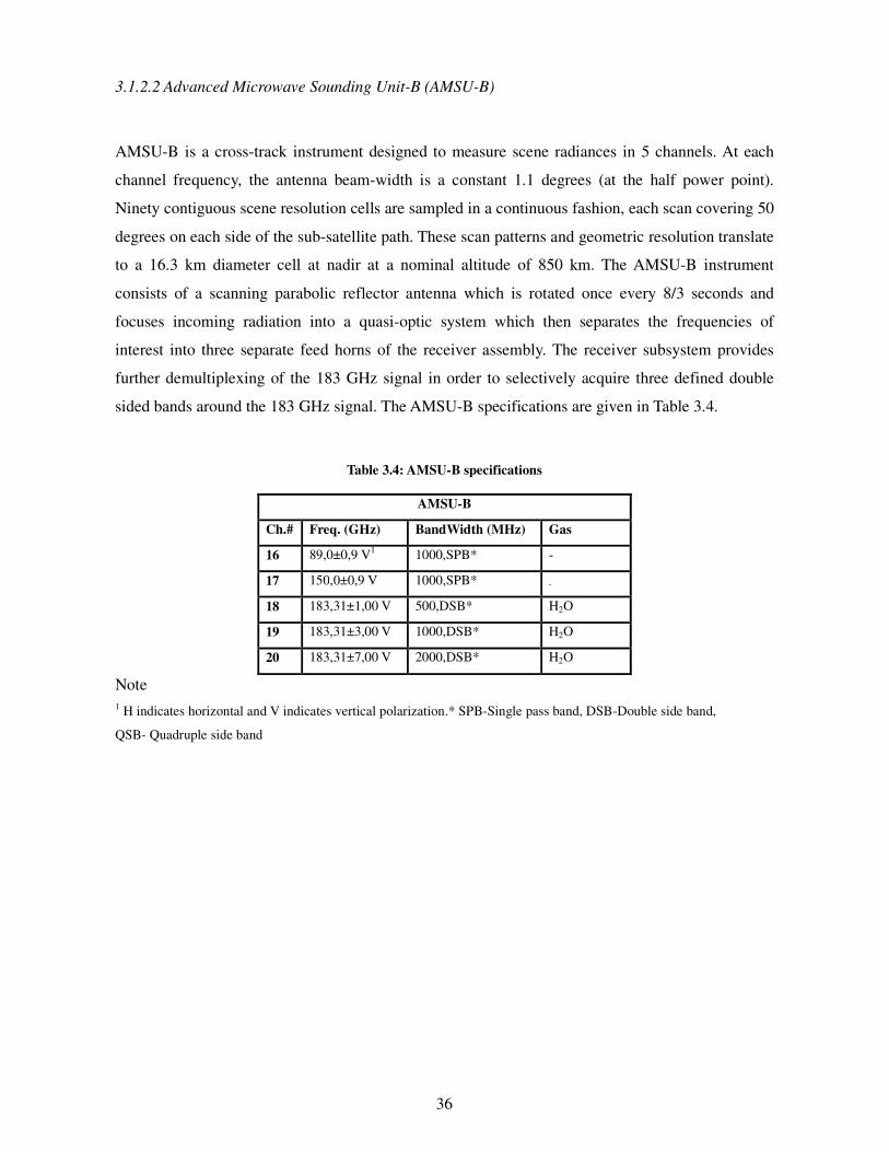
3.1.2.2 Advanced Microwave Sounding Unit-B (AMSU-B)
AMSU-B is a cross-track instrument designed to measure scene radiances in 5 channels. At each
channel frequency, the antenna beam-width is a constant 1.1 degrees (at the half power point).
Ninety contiguous scene resolution cells are sampled in a continuous fashion, each scan covering 50
degrees on each side of the sub-satellite path. These scan patterns and geometric resolution translate
to a 16.3 km diameter cell at nadir at a nominal altitude of 850 km. The AMSU-B instrument
consists of a scanning parabolic reflector antenna which is rotated once every 8/3 seconds and
focuses incoming radiation into a quasi-optic system which then separates the frequencies of
interest into three separate feed horns of the receiver assembly. The receiver subsystem provides
further demultiplexing of the 183 GHz signal in order to selectively acquire three defined double
sided bands around the 183 GHz signal. The AMSU-B specifications are given in Table 3.4.
Table 3.4: AMSU-B specifications
AMSU-B
Ch.# Freq. (GHz) BandWidth (MHz) Gas
16 89,0±0,9 V1
1000,SPB* -
17 150,0±0,9 V 1000,SPB* -
18 183,31±1,00 V 500,DSB* H2O
19 183,31±3,00 V 1000,DSB* H2O
20 183,31±7,00 V 2000,DSB* H2O
Note
1 H indicates horizontal and V indicates vertical polarization.* SPB-Single pass band, DSB-Double side band,
QSB- Quadruple side band
37
3.2 GROUND BASED SENSORS SIMULATIONS
From the data-set collected in WVIOP2004 experiment, a subset of 2 cases of study have been
selected:
1)Clear sky (2004/03/15 23 UTC)
2)Dual-layer cloud (2004/04/04 17 UTC)
For each case the radiative transfer model LBLMS will be used to firstly simulate the measurements
taken from the ground and then those taken from satellites. Simulations of downwelling radiance
permit, in fact, to neglect surface contribution, reducing the uncertainties and focusing on the
atmospheric contribution. Once the model has been tested in up-looking geometry, the up-welling
radiances will be simulate highlighting the importance of a good surface modeling in particular in
presence of ice or snow.
3.2.1 Case study 1: Clear sky conditions
During the 15th of March 2004, four radiosondes have been launched at 23 UTC. For this study the
one that was launched at the “Great White” where the ground radiometers were deployed, has been
selected, defined by Mattioli et al [2007] as the GW-RS90.
The RS90-A is a “PTU-only” system, that is the primary measurements are pressure (P),
temperature (T), and relative humidity (RH). Altitude and dew-point temperature are derived
quantities in the data. The sensor for the temperature measurement is the Vaisala F-Thermocap,
which consists of a capacitive wire. The sensor for the relative humidity is the Vaisala Heated H-
Humicap, a thin film capacitor with a heated twin-sensor design; two humidity sensors work in
phase so that while one sensor is measuring, the other is heated to prevent ice formation (see online
at www.vaisala.com). Samples were taken every 2 s. Details of the sensors’ accuracies are given in
Paukkunen et al. [2001].
38
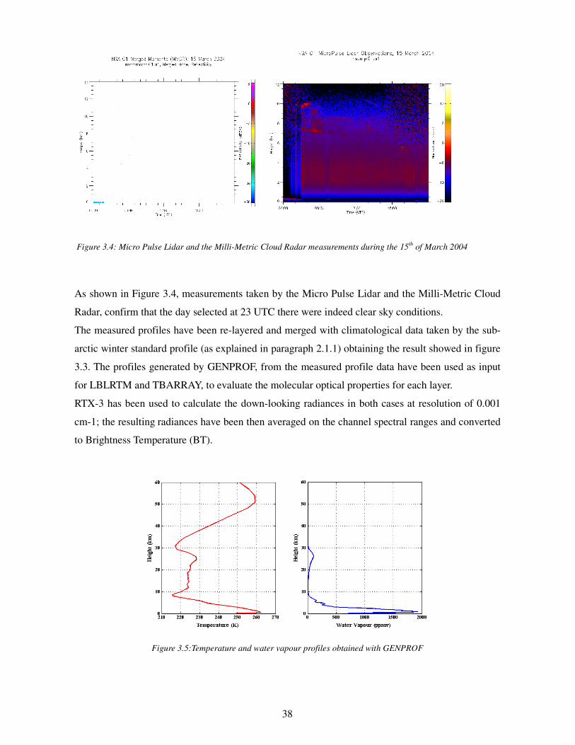
As shown in Figure 3.4, measurements taken by the Micro Pulse Lidar and the Milli-Metric Cloud
Radar, confirm that the day selected at 23 UTC there were indeed clear sky conditions.
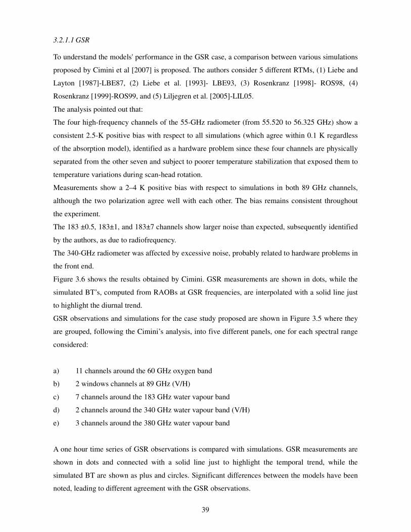
The measured profiles have been re-layered and merged with climatological data taken by the sub-
arctic winter standard profile (as explained in paragraph 2.1.1) obtaining the result showed in figure
3.3. The profiles generated by GENPROF, from the measured profile data have been used as input
for LBLRTM and TBARRAY, to evaluate the molecular optical properties for each layer.
RTX-3 has been used to calculate the down-looking radiances in both cases at resolution of 0.001
cm-1; the resulting radiances have been then averaged on the channel spectral ranges and converted
to Brightness Temperature (BT).
Figure 3.5:Temperature and water vapour profiles obtained with GENPROF
Figure 3.4: Micro Pulse Lidar and the Milli-Metric Cloud Radar measurements during the 15th
of March 2004
39
3.2.1.1 GSR
To understand the models' performance in the GSR case, a comparison between various simulations
proposed by Cimini et al [2007] is proposed. The authors consider 5 different RTMs, (1) Liebe and
Layton [1987]-LBE87, (2) Liebe et al. [1993]- LBE93, (3) Rosenkranz [1998]- ROS98, (4)
Rosenkranz [1999]-ROS99, and (5) Liljegren et al. [2005]-LIL05.
The analysis pointed out that:
The four high-frequency channels of the 55-GHz radiometer (from 55.520 to 56.325 GHz) show a
consistent 2.5-K positive bias with respect to all simulations (which agree within 0.1 K regardless
of the absorption model), identified as a hardware problem since these four channels are physically
separated from the other seven and subject to poorer temperature stabilization that exposed them to
temperature variations during scan-head rotation.
Measurements show a 2–4 K positive bias with respect to simulations in both 89 GHz channels,
although the two polarization agree well with each other. The bias remains consistent throughout
the experiment.
The 183 ±0.5, 183±1, and 183±7 channels show larger noise than expected, subsequently identified
by the authors, as due to radiofrequency.
The 340-GHz radiometer was affected by excessive noise, probably related to hardware problems in
the front end.
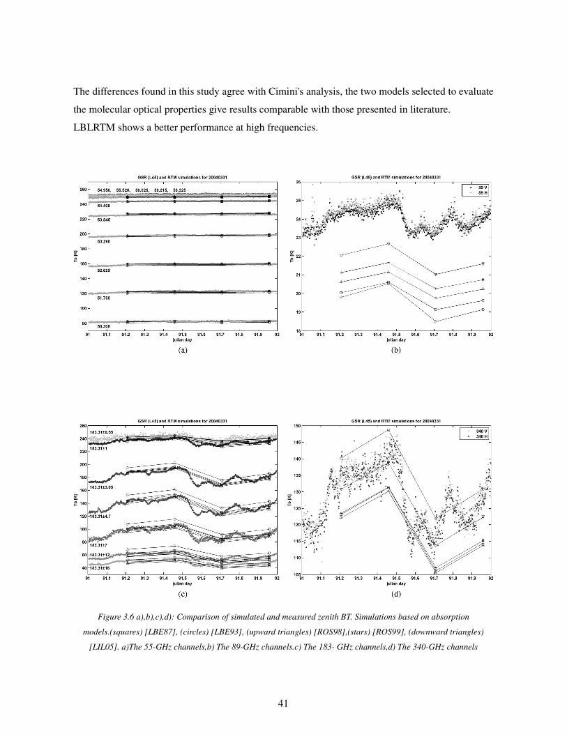
Figure 3.6 shows the results obtained by Cimini. GSR measurements are shown in dots, while the
simulated BT’s, computed from RAOBs at GSR frequencies, are interpolated with a solid line just
to highlight the diurnal trend.
GSR observations and simulations for the case study proposed are shown in Figure 3.5 where they
are grouped, following the Cimini’s analysis, into five different panels, one for each spectral range
considered:
a) 11 channels around the 60 GHz oxygen band
b) 2 windows channels at 89 GHz (V/H)
c) 7 channels around the 183 GHz water vapour band
d) 2 channels around the 340 GHz water vapour band (V/H)
e) 3 channels around the 380 GHz water vapour band
A one hour time series of GSR observations is compared with simulations. GSR measurements are
shown in dots and connected with a solid line just to highlight the temporal trend, while the
simulated BT are shown as plus and circles. Significant differences between the models have been
noted, leading to different agreement with the GSR observations.
40
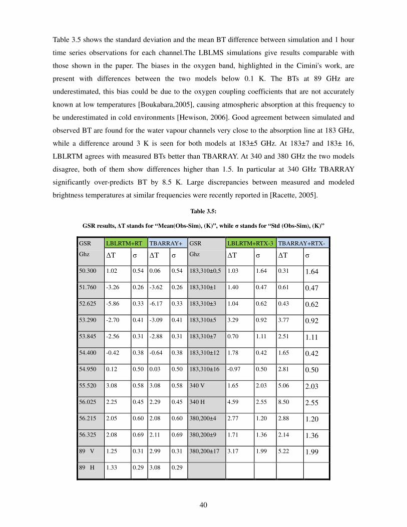
Table 3.5 shows the standard deviation and the mean BT difference between simulation and 1 hour
time series observations for each channel.The LBLMS simulations give results comparable with
those shown in the paper. The biases in the oxygen band, highlighted in the Cimini's work, are
present with differences between the two models below 0.1 K. The BTs at 89 GHz are
underestimated, this bias could be due to the oxygen coupling coefficients that are not accurately
known at low temperatures [Boukabara,2005], causing atmospheric absorption at this frequency to
be underestimated in cold environments [Hewison, 2006]. Good agreement between simulated and
observed BT are found for the water vapour channels very close to the absorption line at 183 GHz,
while a difference around 3 K is seen for both models at 183±5 GHz. At 183±7 and 183± 16,
LBLRTM agrees with measured BTs better than TBARRAY. At 340 and 380 GHz the two models
disagree, both of them show differences higher than 1.5. In particular at 340 GHz TBARRAY
significantly over-predicts BT by 8.5 K. Large discrepancies between measured and modeled
brightness temperatures at similar frequencies were recently reported in [Racette, 2005].
Table 3.5:
GSR results, ∆T stands for “Mean(Obs-Sim), (K)”, while σ stands for “Std (Obs-Sim), (K)”
GSR
Ghz
LBLRTM+RT TBARRAY+ GSR
Ghz
LBLRTM+RTX-3 TBARRAY+RTX-
∆T σ ∆T σ ∆T σ ∆T σ
50.300 1.02 0.54 0.06 0.54 183,310±0,5 1.03 1.64 0.31 1.64
51.760 -3.26 0.26 -3.62 0.26 183,310±1 1.40 0.47 0.61 0.47
52.625 -5.86 0.33 -6.17 0.33 183,310±3 1.04 0.62 0.43 0.62
53.290 -2.70 0.41 -3.09 0.41 183,310±5 3.29 0.92 3.77 0.92
53.845 -2.56 0.31 -2.88 0.31 183,310±7 0.70 1.11 2.51 1.11
54.400 -0.42 0.38 -0.64 0.38 183,310±12 1.78 0.42 1.65 0.42
54.950 0.12 0.50 0.03 0.50 183,310±16 -0.97 0.50 2.81 0.50
55.520 3.08 0.58 3.08 0.58 340 V 1.65 2.03 5.06 2.03
56.025 2.25 0.45 2.29 0.45 340 H 4.59 2.55 8.50 2.55
56.215 2.05 0.60 2.08 0.60 380,200±4 2.77 1.20 2.88 1.20
56.325 2.08 0.69 2.11 0.69 380,200±9 1.71 1.36 2.14 1.36
89 V 1.25 0.31 2.99 0.31 380,200±17 3.17 1.99 5.22 1.99
89 H 1.33 0.29 3.08 0.29
41
The differences found in this study agree with Cimini's analysis, the two models selected to evaluate
the molecular optical properties give results comparable with those presented in literature.
LBLRTM shows a better performance at high frequencies.
Figure 3.6 a),b),c),d): Comparison of simulated and measured zenith BT. Simulations based on absorption
models.(squares) [LBE87], (circles) [LBE93], (upward triangles) [ROS98],(stars) [ROS99], (downward triangles)
[LIL05]. a)The 55-GHz channels,b) The 89-GHz channels.c) The 183- GHz channels,d) The 340-GHz channels
42
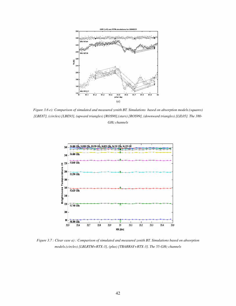
Figure 3.6 e): Comparison of simulated and measured zenith BT. Simulations based on absorption models.(squares)
[LBE87], (circles) [LBE93], (upward triangles) [ROS98],(stars) [ROS99], (downward triangles) [LIL05]. The 380-
GHz channels
Figure 3.7 : Clear case a) : Comparison of simulated and measured zenith BT. Simulations based on absorption
models.(circles) [LBLRTM+RTX-3], (plus) [TBARRAY+RTX-3]. The 55-GHz channels
43
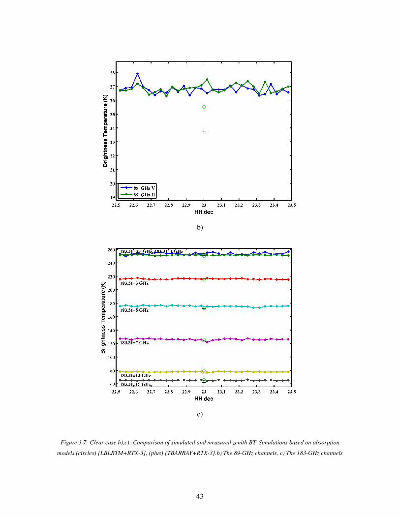
b)
c)
Figure 3.7: Clear case b),c): Comparison of simulated and measured zenith BT. Simulations based on absorption
models.(circles) [LBLRTM+RTX-3], (plus) [TBARRAY+RTX-3].b) The 89-GHz channels, c) The 183-GHz channels
44
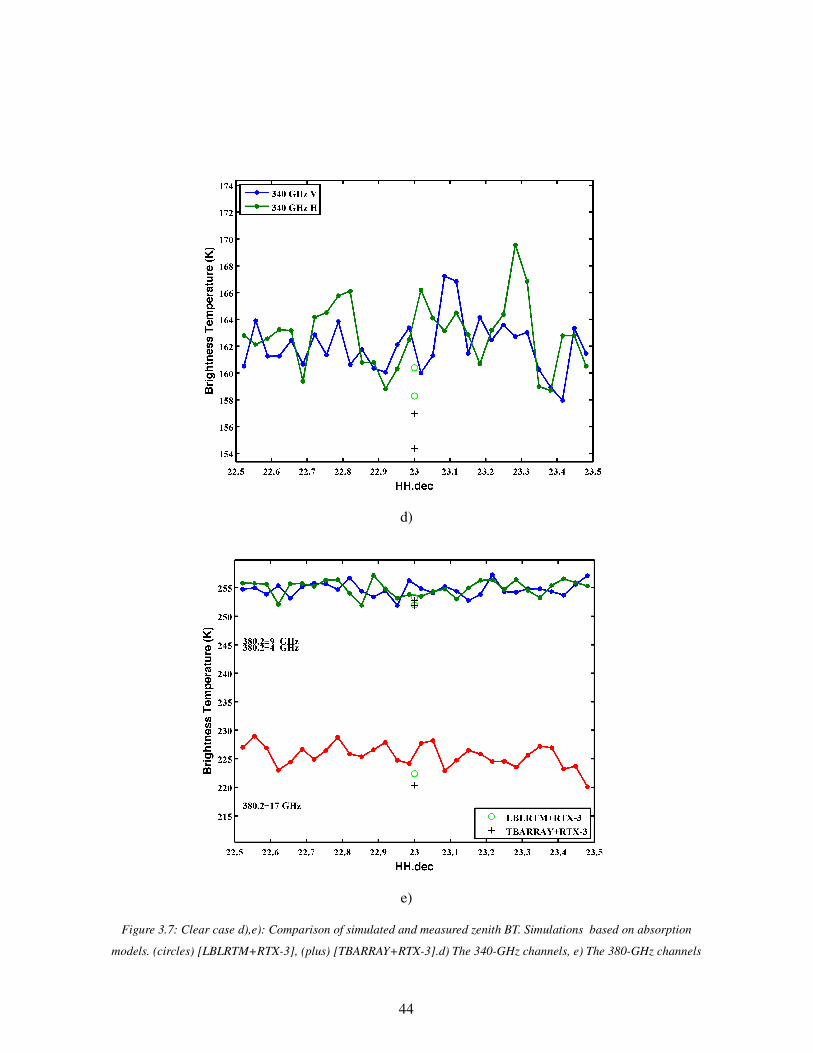
d)
e)
Figure 3.7: Clear case d),e): Comparison of simulated and measured zenith BT. Simulations based on absorption
models. (circles) [LBLRTM+RTX-3], (plus) [TBARRAY+RTX-3].d) The 340-GHz channels, e) The 380-GHz channels
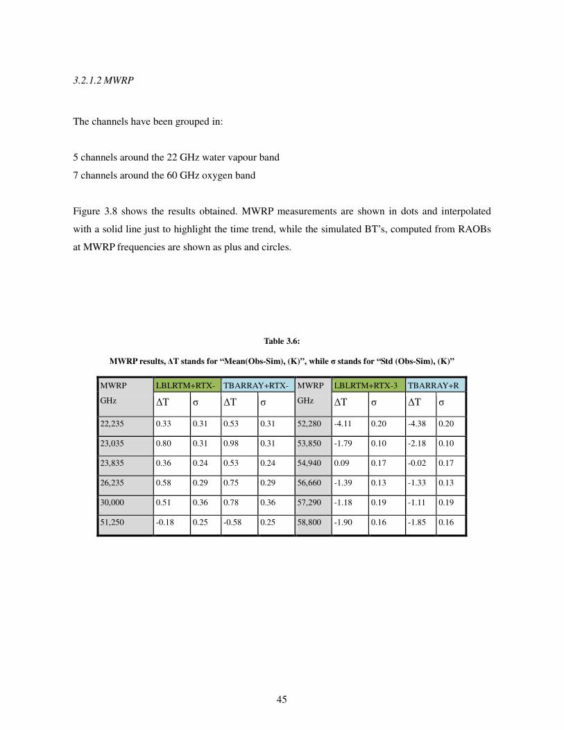
45
3.2.1.2 MWRP
The channels have been grouped in:
5 channels around the 22 GHz water vapour band
7 channels around the 60 GHz oxygen band
Figure 3.8 shows the results obtained. MWRP measurements are shown in dots and interpolated
with a solid line just to highlight the time trend, while the simulated BT’s, computed from RAOBs
at MWRP frequencies are shown as plus and circles.
Table 3.6:
MWRP results, ∆T stands for “Mean(Obs-Sim), (K)”, while σ stands for “Std (Obs-Sim), (K)”
MWRP
GHz
LBLRTM+RTX- TBARRAY+RTX- MWRP
GHz
LBLRTM+RTX-3 TBARRAY+R
∆T σ ∆T σ ∆T σ ∆T σ
22,235 0.33 0.31 0.53 0.31 52,280 -4.11 0.20 -4.38 0.20
23,035 0.80 0.31 0.98 0.31 53,850 -1.79 0.10 -2.18 0.10
23,835 0.36 0.24 0.53 0.24 54,940 0.09 0.17 -0.02 0.17
26,235 0.58 0.29 0.75 0.29 56,660 -1.39 0.13 -1.33 0.13
30,000 0.51 0.36 0.78 0.36 57,290 -1.18 0.19 -1.11 0.19
51,250 -0.18 0.25 -0.58 0.25 58,800 -1.90 0.16 -1.85 0.16
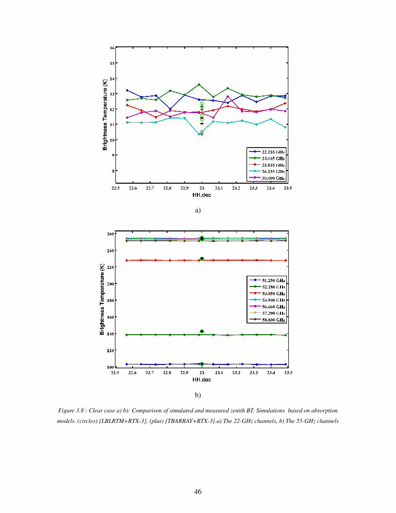
46
a)
b)
Figure 3.8 : Clear case a) b): Comparison of simulated and measured zenith BT. Simulations based on absorption
models. (circles) [LBLRTM+RTX-3], (plus) [TBARRAY+RTX-3].a) The 22-GHz channels, b) The 55-GHz channels
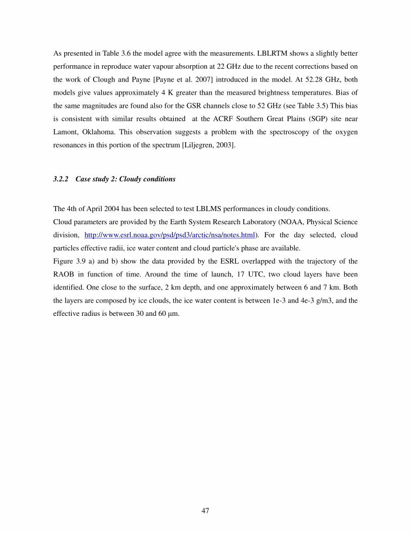
47
As presented in Table 3.6 the model agree with the measurements. LBLRTM shows a slightly better
performance in reproduce water vapour absorption at 22 GHz due to the recent corrections based on
the work of Clough and Payne [Payne et al. 2007] introduced in the model. At 52.28 GHz, both
models give values approximately 4 K greater than the measured brightness temperatures. Bias of
the same magnitudes are found also for the GSR channels close to 52 GHz (see Table 3.5) This bias
is consistent with similar results obtained at the ACRF Southern Great Plains (SGP) site near
Lamont, Oklahoma. This observation suggests a problem with the spectroscopy of the oxygen
resonances in this portion of the spectrum [Liljegren, 2003].
3.2.2 Case study 2: Cloudy conditions
The 4th of April 2004 has been selected to test LBLMS performances in cloudy conditions.
Cloud parameters are provided by the Earth System Research Laboratory (NOAA, Physical Science
division, http://www.esrl.noaa.gov/psd/psd3/arctic/nsa/notes.html). For the day selected, cloud
particles effective radii, ice water content and cloud particle's phase are available.
Figure 3.9 a) and b) show the data provided by the ESRL overlapped with the trajectory of the
RAOB in function of time. Around the time of launch, 17 UTC, two cloud layers have been
identified. One close to the surface, 2 km depth, and one approximately between 6 and 7 km. Both
the layers are composed by ice clouds, the ice water content is between 1e-3 and 4e-3 g/m3, and the
effective radius is between 30 and 60 µm.
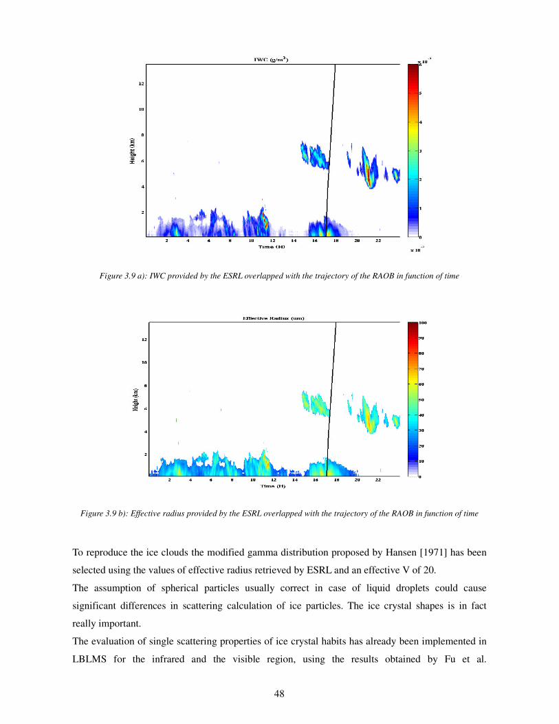
48
Figure 3.9 a): IWC provided by the ESRL overlapped with the trajectory of the RAOB in function of time
Figure 3.9 b): Effective radius provided by the ESRL overlapped with the trajectory of the RAOB in function of time
To reproduce the ice clouds the modified gamma distribution proposed by Hansen [1971] has been
selected using the values of effective radius retrieved by ESRL and an effective V of 20.
The assumption of spherical particles usually correct in case of liquid droplets could cause
significant differences in scattering calculation of ice particles. The ice crystal shapes is in fact
really important.
The evaluation of single scattering properties of ice crystal habits has already been implemented in
LBLMS for the infrared and the visible region, using the results obtained by Fu et al.
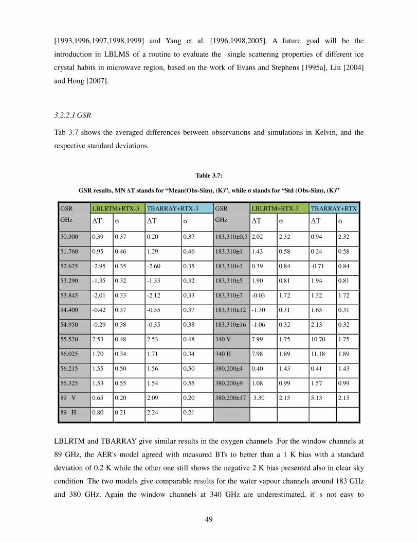
49
[1993,1996,1997,1998,1999] and Yang et al. [1996,1998,2005]. A future goal will be the
introduction in LBLMS of a routine to evaluate the single scattering properties of different ice
crystal habits in microwave region, based on the work of Evans and Stephens [1995a], Liu [2004]
and Hong [2007].
3.2.2.1 GSR
Tab 3.7 shows the averaged differences between observations and simulations in Kelvin, and the
respective standard deviations.
Table 3.7:
GSR results, MN ∆T stands for “Mean(Obs-Sim), (K)”, while σ stands for “Std (Obs-Sim), (K)”
GSR
GHz
LBLRTM+RTX-3 TBARRAY+RTX-3 GSR
GHz
LBLRTM+RTX-3 TBARRAY+RTX
∆T σ ∆T σ ∆T σ ∆T σ
50.300 0.39 0.37 0.20 0.37 183,310±0,5 2.02 2.32 0.94 2.32
51.760 0.95 0.46 1.29 0.46 183,310±1 1.43 0.58 0.24 0.58
52.625 -2.95 0.35 -2.60 0.35 183,310±3 0.39 0.84 -0.71 0.84
53.290 -1.35 0.32 -1.33 0.32 183,310±5 1.90 0.81 1.94 0.81
53.845 -2.01 0.33 -2.12 0.33 183,310±7 -0.03 1.72 1.32 1.72
54.400 -0.42 0.37 -0.55 0.37 183,310±12 -1.30 0.31 1.65 0.31
54.950 -0.29 0.38 -0.35 0.38 183,310±16 -1.06 0.32 2.13 0.32
55.520 2.53 0.48 2.53 0.48 340 V 7.99 1.75 10.70 1.75
56.025 1.70 0.34 1.71 0.34 340 H 7.98 1.89 11.18 1.89
56.215 1.55 0.50 1.56 0.50 380,200±4 0.40 1.43 0.41 1.43
56.325 1.53 0.55 1.54 0.55 380,200±9 1.08 0.99 1.57 0.99
89 V 0.65 0.20 2.09 0.20 380,200±17 3.30 2.15 5.13 2.15
89 H 0.80 0.21 2.24 0.21
LBLRTM and TBARRAY give similar results in the oxygen channels .For the window channels at
89 GHz, the AER's model agreed with measured BTs to better than a 1 K bias with a standard
deviation of 0.2 K while the other one still shows the negative 2 K bias presented also in clear sky
condition. The two models give comparable results for the water vapour channels around 183 GHz
and 380 GHz. Again the window channels at 340 GHz are underestimated, it' s not easy to
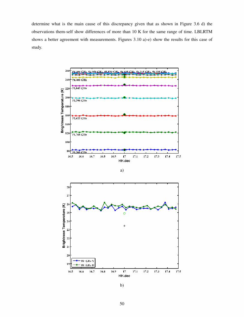
50
determine what is the main cause of this discrepancy given that as shown in Figure 3.6 d) the
observations them-self show differences of more than 10 K for the same range of time. LBLRTM
shows a better agreement with measurements. Figures 3.10 a)-e) show the results for this case of
study.
a)
b)
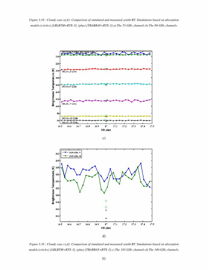
51
Figure 3.10 : Cloudy case a),b): Comparison of simulated and measured zenith BT. Simulations based on absorption
models.(circles) [LBLRTM+RTX-3], (plus) [TBARRAY+RTX-3].a) The 55-GHz channels b) The 89-GHz channels.
c)
d)
Figure 3.10 : Cloudy case c),d): Comparison of simulated and measured zenith BT. Simulations based on absorption
models.(circles) [LBLRTM+RTX-3], (plus) [TBARRAY+RTX-3].c) The 183-GHz channels d) The 340-GHz channels.
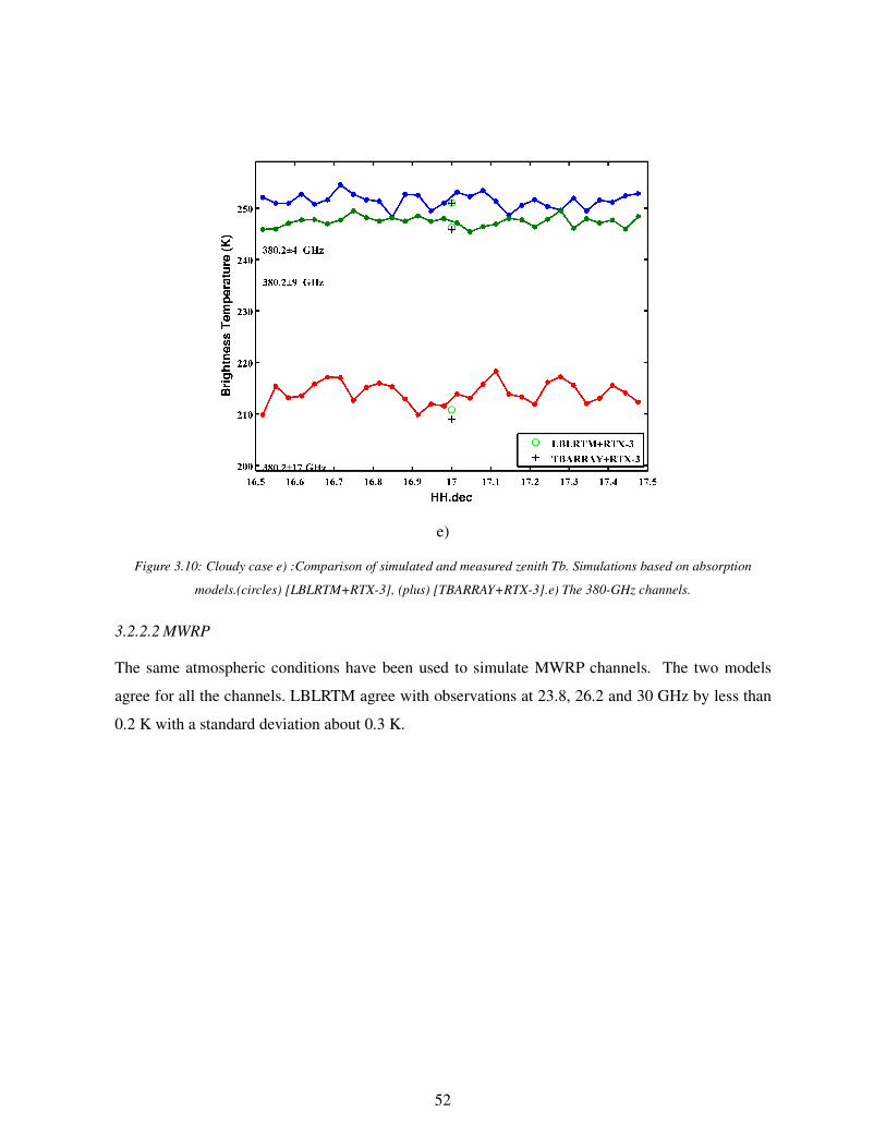
52
e)
Figure 3.10: Cloudy case e) :Comparison of simulated and measured zenith Tb. Simulations based on absorption
models.(circles) [LBLRTM+RTX-3], (plus) [TBARRAY+RTX-3].e) The 380-GHz channels.
3.2.2.2 MWRP
The same atmospheric conditions have been used to simulate MWRP channels. The two models
agree for all the channels. LBLRTM agree with observations at 23.8, 26.2 and 30 GHz by less than
0.2 K with a standard deviation about 0.3 K.
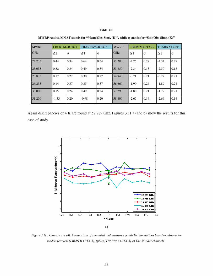
53
Table 3.8:
MWRP results, MN ∆T stands for “Mean(Obs-Sim), (K)”, while σ stands for “Std (Obs-Sim), (K)”
MWRP
GHz
LBLRTM+RTX-3 TBARRAY+RTX-3 MWRP
GHz
LBLRTM+RTX-3 TBARRAY+RT
∆T σ ∆T σ ∆T σ ∆T σ
22,235 0.44 0.34 0.64 0.34 52,280 -4.75 0.29 -4.34 0.29
23,035 0.32 0.34 0.49 0.34 53,850 -2.34 0.18 -2.50 0.18
23,835 0.12 0.22 0.30 0.22 54,940 -0.21 0.21 -0.27 0.21
26,235 0.14 0.37 0.35 0.37 56,660 -1.90 0.24 -1.89 0.24
30,000 0.15 0.24 0.49 0.24 57,290 -1.80 0.21 -1.79 0.21
51,250 -1.33 0.20 -0.98 0.20 58,800 -2.67 0.14 -2.66 0.14
Again discrepancies of 4 K are found at 52.289 Ghz. Figures 3.11 a) and b) show the results for this
case of study.
a)
Figure 3.11 : Cloudy case a)): Comparison of simulated and measured zenith Tb. Simulations based on absorption
models.(circles) [LBLRTM+RTX-3], (plus) [TBARRAY+RTX-3].a) The 55-GHz channels .
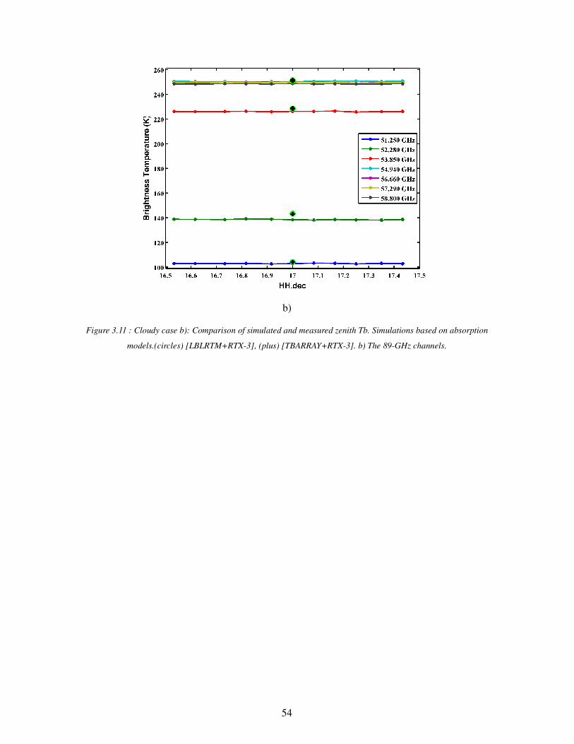
54
b)
Figure 3.11 : Cloudy case b): Comparison of simulated and measured zenith Tb. Simulations based on absorption
models.(circles) [LBLRTM+RTX-3], (plus) [TBARRAY+RTX-3]. b) The 89-GHz channels.
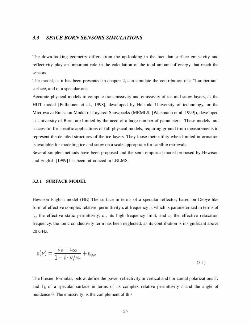
55
3.3 SPACE BORN SENSORS SIMULATIONS
The down-looking geometry differs from the up-looking in the fact that surface emissivity and
reflectivity play an important role in the calculation of the total amount of energy that reach the
sensors.
The model, as it has been presented in chapter 2, can simulate the contribution of a “Lambertian”
surface, and of a specular one.
Accurate physical models to compute transmissivity and emissivity of ice and snow layers, as the
HUT model [Pulliainen et al., 1998], developed by Helsinki University of technology, or the
Microwave Emission Model of Layered Snowpacks (MEMLS, [Weismann et al.,1999]), developed
at University of Bern, are limited by the need of a large number of parameters. These models are
successful for specific applications of full physical models, requiring ground truth measurements to
represent the detailed structures of the ice layers. They loose their utility when limited information
is available for modeling ice and snow on a scale appropriate for satellite retrievals.
Several simpler methods have been proposed and the semi-empirical model proposed by Hewison
and English [1999] has been introduced in LBLMS.
3.3.1 SURFACE MODEL
Hewison-English model (HE) The surface in terms of a specular reflector, based on Debye-like
form of effective complex relative permittivity ε at frequency υ, which is parameterized in terms of
εs, the effective static permittivity, ε∞, its high frequency limit, and υr the effective relaxation
frequency. the ionic conductivity term has been neglected, as its contribution is insignificant above
20 GHz.
(3.1)
The Fresnel formulas, below, define the power reflectivity in vertical and horizontal polarizations Γv
and Γh of a specular surface in terms of its complex relative permittivity ε and the angle of
incidence θ. The emissivity is the complement of this
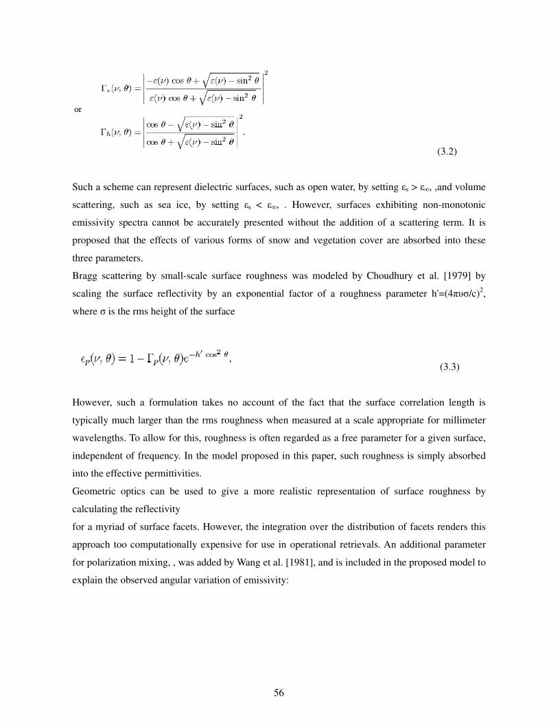
56
(3.2)
Such a scheme can represent dielectric surfaces, such as open water, by setting εs > ε∞, ,and volume
scattering, such as sea ice, by setting εs < ε∞, . However, surfaces exhibiting non-monotonic
emissivity spectra cannot be accurately presented without the addition of a scattering term. It is
proposed that the effects of various forms of snow and vegetation cover are absorbed into these
three parameters.
Bragg scattering by small-scale surface roughness was modeled by Choudhury et al. [1979] by
scaling the surface reflectivity by an exponential factor of a roughness parameter h'=(4πυσ/c)2,
where σ is the rms height of the surface
(3.3)
However, such a formulation takes no account of the fact that the surface correlation length is
typically much larger than the rms roughness when measured at a scale appropriate for millimeter
wavelengths. To allow for this, roughness is often regarded as a free parameter for a given surface,
independent of frequency. In the model proposed in this paper, such roughness is simply absorbed
into the effective permittivities.
Geometric optics can be used to give a more realistic representation of surface roughness by
calculating the reflectivity
for a myriad of surface facets. However, the integration over the distribution of facets renders this
approach too computationally expensive for use in operational retrievals. An additional parameter
for polarization mixing, , was added by Wang et al. [1981], and is included in the proposed model to
explain the observed angular variation of emissivity:
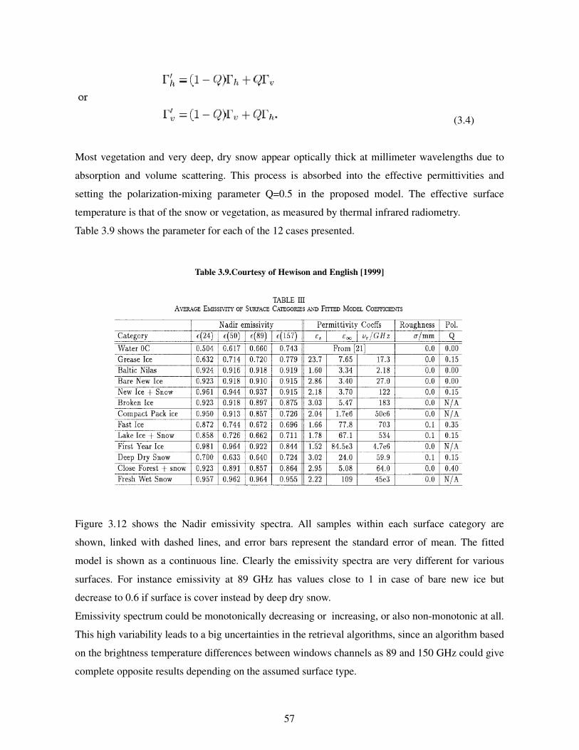
57
(3.4)
Most vegetation and very deep, dry snow appear optically thick at millimeter wavelengths due to
absorption and volume scattering. This process is absorbed into the effective permittivities and
setting the polarization-mixing parameter Q=0.5 in the proposed model. The effective surface
temperature is that of the snow or vegetation, as measured by thermal infrared radiometry.
Table 3.9 shows the parameter for each of the 12 cases presented.
Table 3.9.Courtesy of Hewison and English [1999]
Figure 3.12 shows the Nadir emissivity spectra. All samples within each surface category are
shown, linked with dashed lines, and error bars represent the standard error of mean. The fitted
model is shown as a continuous line. Clearly the emissivity spectra are very different for various
surfaces. For instance emissivity at 89 GHz has values close to 1 in case of bare new ice but
decrease to 0.6 if surface is cover instead by deep dry snow.
Emissivity spectrum could be monotonically decreasing or increasing, or also non-monotonic at all.
This high variability leads to a big uncertainties in the retrieval algorithms, since an algorithm based
on the brightness temperature differences between windows channels as 89 and 150 GHz could give
complete opposite results depending on the assumed surface type.
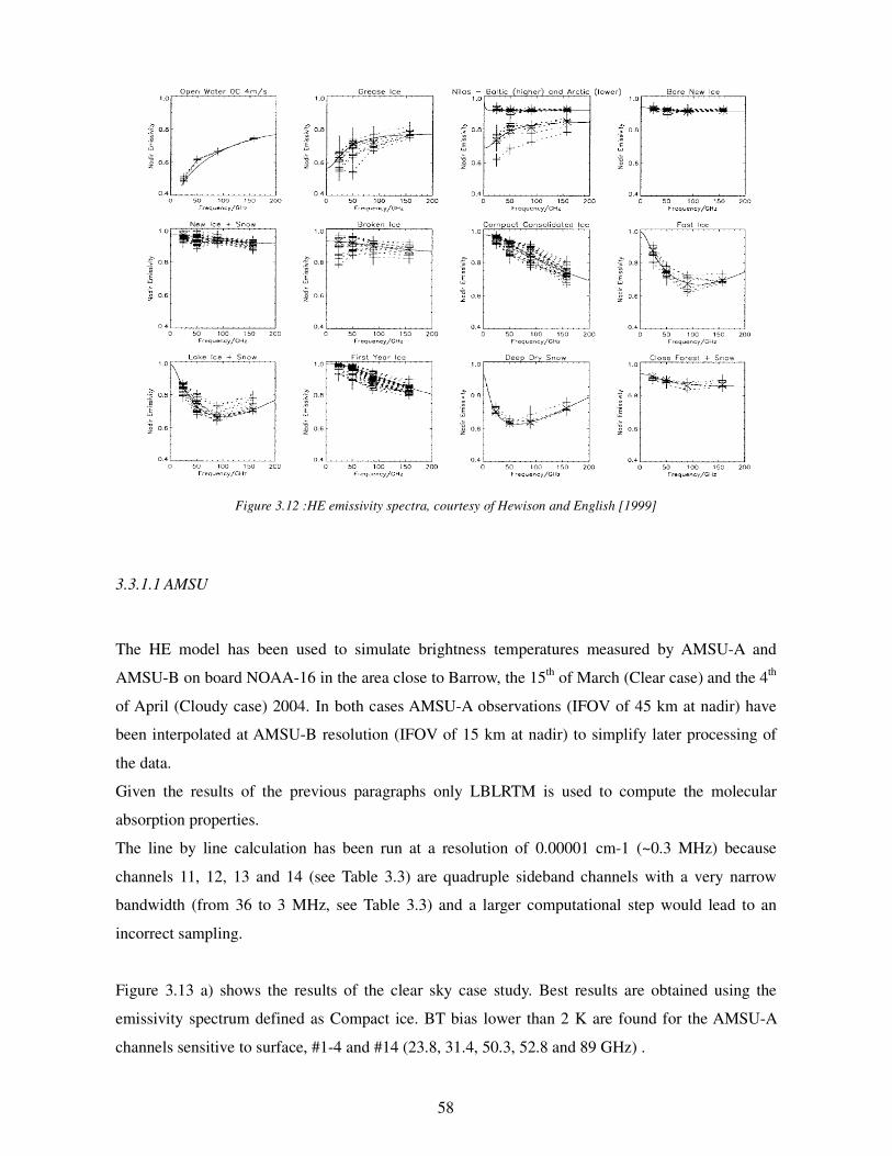
58
Figure 3.12 :HE emissivity spectra, courtesy of Hewison and English [1999]
3.3.1.1 AMSU
The HE model has been used to simulate brightness temperatures measured by AMSU-A and
AMSU-B on board NOAA-16 in the area close to Barrow, the 15th
of March (Clear case) and the 4th
of April (Cloudy case) 2004. In both cases AMSU-A observations (IFOV of 45 km at nadir) have
been interpolated at AMSU-B resolution (IFOV of 15 km at nadir) to simplify later processing of
the data.
Given the results of the previous paragraphs only LBLRTM is used to compute the molecular
absorption properties.
The line by line calculation has been run at a resolution of 0.00001 cm-1 (~0.3 MHz) because
channels 11, 12, 13 and 14 (see Table 3.3) are quadruple sideband channels with a very narrow
bandwidth (from 36 to 3 MHz, see Table 3.3) and a larger computational step would lead to an
incorrect sampling.
Figure 3.13 a) shows the results of the clear sky case study. Best results are obtained using the
emissivity spectrum defined as Compact ice. BT bias lower than 2 K are found for the AMSU-A
channels sensitive to surface, #1-4 and #14 (23.8, 31.4, 50.3, 52.8 and 89 GHz) .
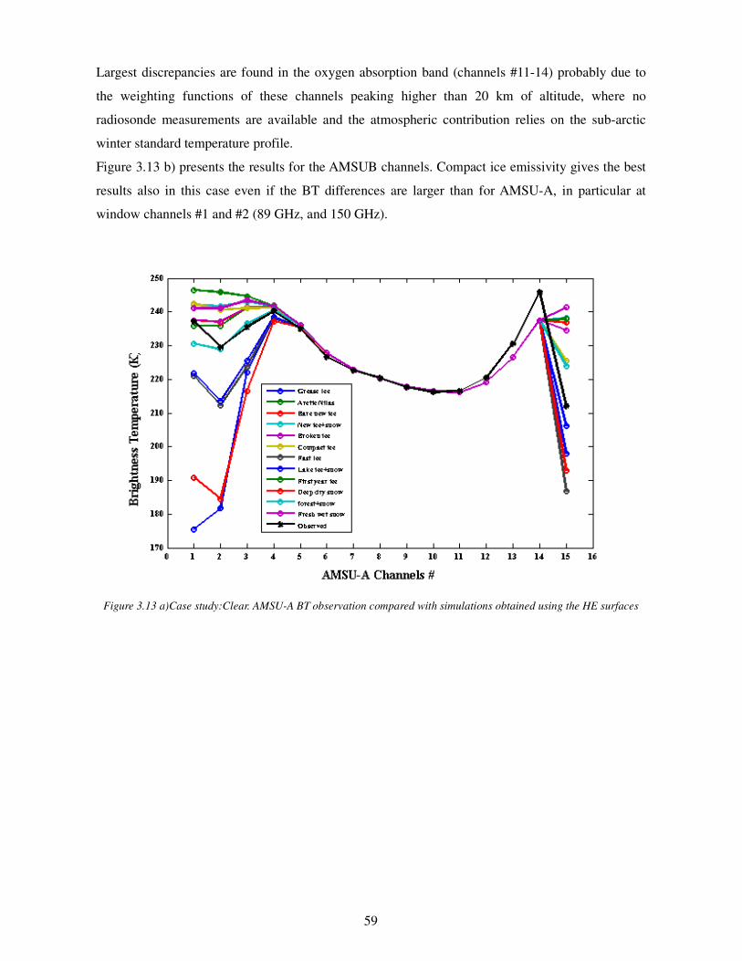
59
Largest discrepancies are found in the oxygen absorption band (channels #11-14) probably due to
the weighting functions of these channels peaking higher than 20 km of altitude, where no
radiosonde measurements are available and the atmospheric contribution relies on the sub-arctic
winter standard temperature profile.
Figure 3.13 b) presents the results for the AMSUB channels. Compact ice emissivity gives the best
results also in this case even if the BT differences are larger than for AMSU-A, in particular at
window channels #1 and #2 (89 GHz, and 150 GHz).
Figure 3.13 a)Case study:Clear. AMSU-A BT observation compared with simulations obtained using the HE surfaces
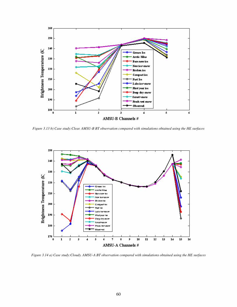
60
Figure 3.13 b) Case study:Clear. AMSU-B BT observation compared with simulations obtained using the HE surfaces
Figure 3.14 a) Case study:Cloudy. AMSU-A BT observation compared with simulations obtained using the HE surfaces
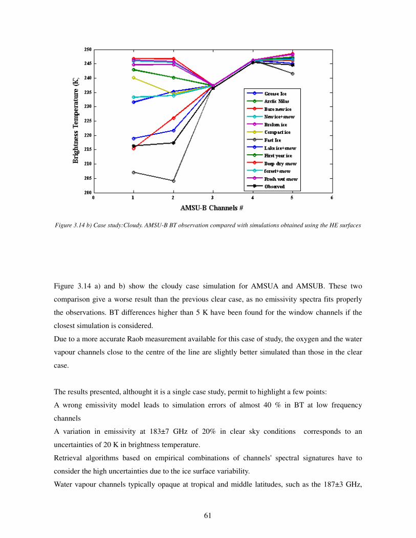
61
Figure 3.14 b) Case study:Cloudy. AMSU-B BT observation compared with simulations obtained using the HE surfaces
Figure 3.14 a) and b) show the cloudy case simulation for AMSUA and AMSUB. These two
comparison give a worse result than the previous clear case, as no emissivity spectra fits properly
the observations. BT differences higher than 5 K have been found for the window channels if the
closest simulation is considered.
Due to a more accurate Raob measurement available for this case of study, the oxygen and the water
vapour channels close to the centre of the line are slightly better simulated than those in the clear
case.
The results presented, althought it is a single case study, permit to highlight a few points:
A wrong emissivity model leads to simulation errors of almost 40 % in BT at low frequency
channels
A variation in emissivity at 183±7 GHz of 20% in clear sky conditions corresponds to an
uncertainties of 20 K in brightness temperature.
Retrieval algorithms based on empirical combinations of channels' spectral signatures have to
consider the high uncertainties due to the ice surface variability.
Water vapour channels typically opaque at tropical and middle latitudes, such as the 187±3 GHz,

62
show a weak sensitivity to surface emissivity
All this points have to be considered in order to understand the difficulty to discriminate a snowing(
or raining) area and a clear area at very high latitudes since signals of the same type could be due to
a snowfall or to a particular surface emissivity spectrum leading to a completely wrong
interpretation.
3.4 DISCUSSION
The new LBLMS has been used to simulate down-welling and up-welling microwave radiances in
Arctic region with results comparable with specific RTMs present in literature. Also if a more
realistic representation of ice cloud particles and precipitating ice crystal is still necessary as well as
a more complete surface model the results are encouraging.
The up-welling simulations have given the opportunity to present few unsolved issues of the remote
sensing of arctic region introducing the high uncertainties due to surface ice or snow covered,.
63
4 A FIRST TENTATIVE: IMPROVING THE SSA ALGORITHM
Although the obtained results obtained in Chapter 3 only relate to a limited number of case studies,
they allow to introduce the difficult problem of the interpretation of space borne measurements over
the poles, and, in particular, of the detection of precipitating areas. Most of the research works
proposed in the literature identify the problem of snowfall detection on polar region as an unsolved
problem. The lack of radar or rain gauge observations has prevented, up to the present, the
evolution of models or algorithms specific for those areas.
Chen et al. [2003] proved the sensitivity of high frequency microwave channels to precipitation,
highlighting their efficiency also in the Arctic region but underlining the risk of wrong detection
when using the water vapour channels in very dry atmospheric conditions. Liu et al. [2002]
identified the scattering signal at 150 GHz channel as the most sensitive to snowfall over ocean at
high latitude. A model of radiation at millimeter-wave frequencies presented by Skofronick-Jackson
et al. [2002] seeks to infer snowfall rates over land, by taking advantage of water vapor screening in
order to obscure the underlying snow-covered surface.
Kongoli and Ferraro[2003] showed that the linear combinations, BT176 (BT at 183.31±7GHz) –
BT180 ( BT at 183.31±3 GHz) and BT150 – BT180, are useful to remove new snow cover
signatures misidentified as snowfall on North America. Unfortunately their method, calibrated on
the North America area, defines thresholds that may lead to large errors at higher latitudes.
Surussavadee and Staelin [Surussavadee and Staelin, 2006, 2007, 2008; Staelin and Surussavadee,
2007] presented a global precipitation retrieval algorithm (defined hereafter SSA) based on AMSU
to estimate surface precipitation rate, peak vertical wind, and water-paths for rainwater, snow,
graupel, cloud water, cloud ice over non-icy land and ocean. The authors show that the algorithm is
able to detect polar storms but also highlight the fact that precipitation retrievals over sea ice or
snow-covered land are difficult because those channels penetrating to the surface have difficulty
distinguishing snow or ice on the ground from icy hydrometeors aloft. Moreover, they found that
even the normally opaque channels near 183,31 GHz can sense the surface when the air is
sufficiently dry, leading to a high percentage of false alarms (estimation of precipitation in clear and
dry conditions).
As previously discussed, the above mentioned approaches are not particularly applicable to the
higher latitudes and, in addition, tend to produce a large number of false alarms. The work proposed
in the following chapter takes its motivation from the relatively large false alarm rate produced by
the SSA in the polar regions with the aim of extending to the difficult cases, namely the detection of
64
the rainy events as a pre-condition to the estimation of the rain rate over snow and ice surfaces.
4.1 SSA
SSA utilizes NOAA AMSU channels 23-191 GHz to estimate the rain rate at global scale.
The MM5/TBSCAT/F(λ) model composed by:
� MM5: a NWP mesoscale cloud-resolving model [Dudhia, 2005], run at 15-km resolution
with NCEP initialization;
� TBSCAT:the Rosenkranz two-stream radiative transfer model (see Chapter 2)
� F(λ):an electromagnetic model for icy hydrometeors (see Chapter 2) .
is used as global precipitation ground truth to train and to validate the algorithm.
Given the nonlinear and imperfectly known relationship between precipitation and satellite
brightness temperatures, SSA employs a neural networks (NN) to retrieve it.
The estimates of surface precipitation rates and hydrometeor water-paths are trained using NCEP-
initialized MM5 simulations of 106 representative storms and their corresponding brightness
temperatures simulated using TBSCAT and the F(λ) approximation at AMSU frequencies. Only
storms with simulated morphologies that match simultaneous AMSU observations near 183±7 GHz
are used for the training.
As it is usually done in Artificial Neural Network approaches, training is followed by verification.
Verification shows that the algorithm, when evaluated against MM5 precipitation forecasts,
performs reasonably well at low and mid-latitudes for all types of precipitation, but, unfortunately,
not at higher latitudes, particularly over snow and ice.
4.1.2 A METHOD TO DETECT FALSE ALARMS
Under the supervision of Professor Staelin and Dr. Rosenkranz of the Remote Sensing and
Estimation Group of the Massachusetts Institute of Technology, a method was developed to detect
those conditions that could lead to an erroneous estimation at higher latitudes. The method is based
on the hypothesis that if high latitude conditions made the channel at 183±7 GHz (far-wing of the
water vapour absorption line) sufficiently opaque for surface effects to be negligible, the SSA
retrievals of surface precipitation rates should retain most of their validity.
To test this hypothesis an algorithm that estimates atmospheric optical depth using NCEP analyses
was written to identify the most transparent areas where unreliable retrievals were expected
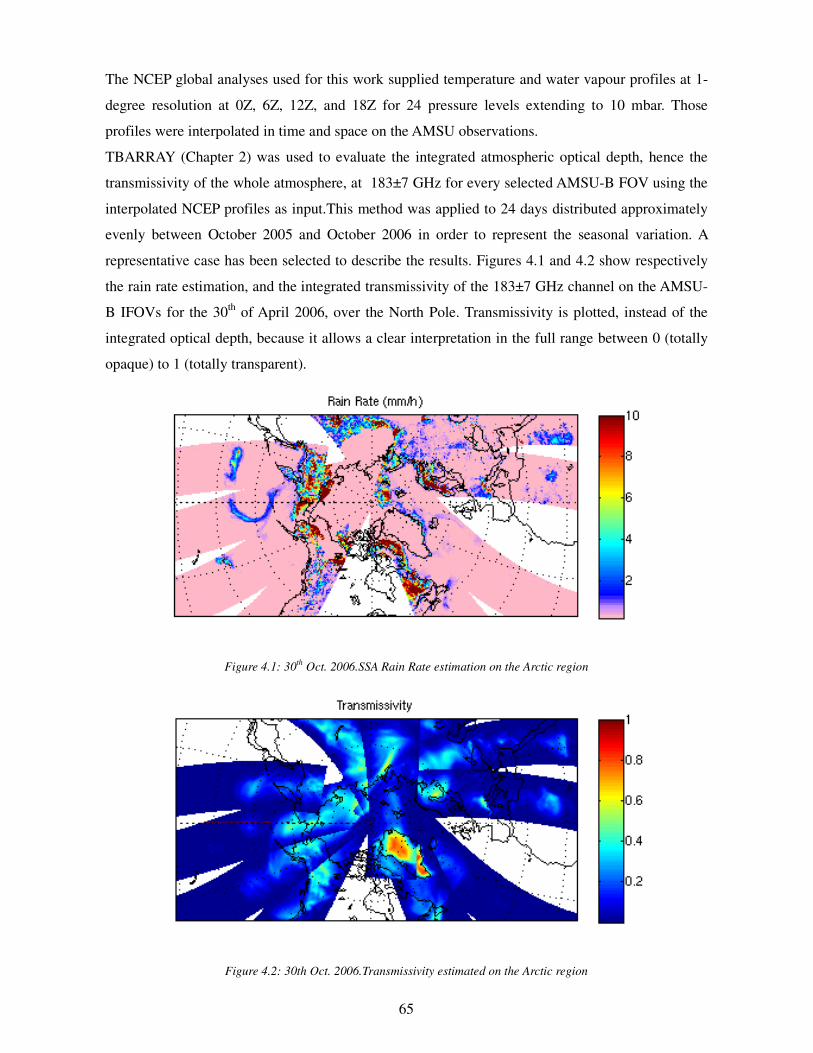
65
The NCEP global analyses used for this work supplied temperature and water vapour profiles at 1-
degree resolution at 0Z, 6Z, 12Z, and 18Z for 24 pressure levels extending to 10 mbar. Those
profiles were interpolated in time and space on the AMSU observations.
TBARRAY (Chapter 2) was used to evaluate the integrated atmospheric optical depth, hence the
transmissivity of the whole atmosphere, at 183±7 GHz for every selected AMSU-B FOV using the
interpolated NCEP profiles as input.This method was applied to 24 days distributed approximately
evenly between October 2005 and October 2006 in order to represent the seasonal variation. A
representative case has been selected to describe the results. Figures 4.1 and 4.2 show respectively
the rain rate estimation, and the integrated transmissivity of the 183±7 GHz channel on the AMSU-
B IFOVs for the 30th
of April 2006, over the North Pole. Transmissivity is plotted, instead of the
integrated optical depth, because it allows a clear interpretation in the full range between 0 (totally
opaque) to 1 (totally transparent).
Figure 4.1: 30th
Oct. 2006.SSA Rain Rate estimation on the Arctic region
Figure 4.2: 30th Oct. 2006.Transmissivity estimated on the Arctic region
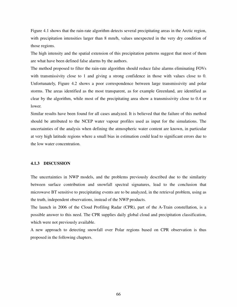
66
Figure 4.1 shows that the rain-rate algorithm detects several precipitating areas in the Arctic region,
with precipitation intensities larger than 8 mm/h, values unexpected in the very dry condition of
those regions.
The high intensity and the spatial extension of this precipitation patterns suggest that most of them
are what have been defined false alarms by the authors.
The method proposed to filter the rain-rate algorithm should reduce false alarms eliminating FOVs
with transmissivity close to 1 and giving a strong confidence in those with values close to 0.
Unfortunately, Figure 4.2 shows a poor correspondence between large transmissivity and polar
storms. The areas identified as the most transparent, as for example Greenland, are identified as
clear by the algorithm, while most of the precipitating area show a transmissivity close to 0.4 or
lower.
Similar results have been found for all cases analyzed. It is believed that the failure of this method
should be attributed to the NCEP water vapour profiles used as input for the simulations. The
uncertainties of the analysis when defining the atmospheric water content are known, in particular
at very high latitude regions where a small bias in estimation could lead to significant errors due to
the low water concentration.
4.1.3 DISCUSSION
The uncertainties in NWP models, and the problems previously described due to the similarity
between surface contribution and snowfall spectral signatures, lead to the conclusion that
microwave BT sensitive to precipitating events are to be analyzed, in the retrieval problem, using as
the truth, independent observations, instead of the NWP products.
The launch in 2006 of the Cloud Profiling Radar (CPR), part of the A-Train constellation, is a
possible answer to this need. The CPR supplies daily global cloud and precipitation classification,
which were not previously available.
A new approach to detecting snowfall over Polar regions based on CPR observation is thus
proposed in the following chapters.
67
5 DEFINING AN ALTERNATIVE APPROACH: MATERIALS AND
METHODS
Given the failure of all the approaches described in Chapter 4, an alternative approach is here
proposed which aims at using passive microwave and infrared measurements as the predictands
which can allow to discriminate between snowing/no-snowing areas. In addition, it is here proposed
to use the observations of the new CPR aboard the platform CloudSat, as the truth to be used for
calibrating and validating the new detection scheme.
5.1 THE DATA USED TO IMPLEMENT THE APPROACH
To implement the new approach, the AMSU-A and B observations from NOAA-16, already
described in Chapter 3, have been complemented by the data collected by MODIS on board of
AQUA.
The decision of introducing additional 11 infrared channels is justified by their reduced sensitivity
to the surface structure. The rationale for this combination is that channels in infrared regions might
complement those in the microwave region with an expected enhancement in the ability of detecting
clear sky conditions.
5.2 THE METHODOLOGICAL APPROACH
The methodological approach can be divided into two different steps. In a first step, following
Kongoli et al. [2003], an empirical search for a threshold aimed at discriminating the case of no
snow was performed. The results of this first approach, although coherent with the ones obtained by
Kongoli et al. [2003], were not fully satisfactorily. As defined in the sequel, only one of the four
possible cases (see Figure 5.1) could be clearly classified (namely the correct negatives).
The problem of defining the presence or not of snow, as it will be explained more deeply in Chapter
6, can be fully represented by a 2x2 contingency table of yes/no events, such as snow/no snow, as
the one presented in Figure 5.1. The elements in the table (hits, misses, false alarms, correct
negatives) are proportional to the joint distribution of events, while the elements below (estimates
yes, estimated no) and to the right (observed yes, observed no) are called the marginal distribution.
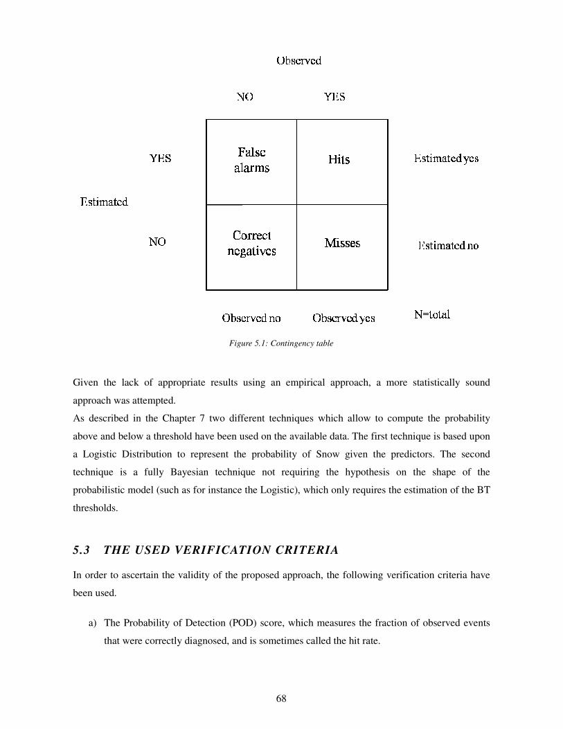
68
Figure 5.1: Contingency table
Given the lack of appropriate results using an empirical approach, a more statistically sound
approach was attempted.
As described in the Chapter 7 two different techniques which allow to compute the probability
above and below a threshold have been used on the available data. The first technique is based upon
a Logistic Distribution to represent the probability of Snow given the predictors. The second
technique is a fully Bayesian technique not requiring the hypothesis on the shape of the
probabilistic model (such as for instance the Logistic), which only requires the estimation of the BT
thresholds.
5.3 THE USED VERIFICATION CRITERIA
In order to ascertain the validity of the proposed approach, the following verification criteria have
been used.
a) The Probability of Detection (POD) score, which measures the fraction of observed events
that were correctly diagnosed, and is sometimes called the hit rate.

69
Hits
POD =Hits Misses+
(5.1)
� The False Alarm Ratio (FAR) score gives the fraction of diagnosed events the were actually
non-events.
False alarms
FAR =Hits False alarms+
(5.1)
Perfect values for this scores are POD=1, and FAR=0. The POD and FAR should always be used in
conjunction.
These validation indexes have been extended to encompass both cases of hits and correct negatives
as it will be described in chapter 7. The proposed approaches were also compared to the SSA results
and found positively performing in terms of the same validation indexes.
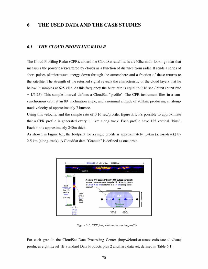
70
6 THE USED DATA AND THE CASE STUDIES
6.1 THE CLOUD PROFILING RADAR
The Cloud Profiling Radar (CPR), aboard the CloudSat satellite, is a 94Ghz nadir looking radar that
measures the power backscattered by clouds as a function of distance from radar. It sends a series of
short pulses of microwave energy down through the atmosphere and a fraction of these returns to
the satellite. The strength of the returned signal reveals the characteristic of the cloud layers that lie
below. It samples at 625 kHz. At this frequency the burst rate is equal to 0.16 sec / burst (burst rate
= 1/6.25). This sample interval defines a CloudSat "profile". The CPR instrument flies in a sun-
synchronous orbit at an 89° inclination angle, and a nominal altitude of 705km, producing an along-
track velocity of approximately 7 km/sec.
Using this velocity, and the sample rate of 0.16 sec/profile, figure 5.1, it's possible to approximate
that a CPR profile is generated every 1.1 km along track. Each profile have 125 vertical "bins".
Each bin is approximately 240m thick.
As shown in Figure 6.1, the footprint for a single profile is approximately 1.4km (across-track) by
2.5 km (along-track). A CloudSat data "Granule" is defined as one orbit.
For each granule the CloudSat Data Processing Center (http://cloudsat.atmos.colostate.edu/data)
produces eight Level 1B Standard Data Products plus 2 ancillary data set, defined in Table 6.1:
Figure 6.1: CPR footprint and scanning profile
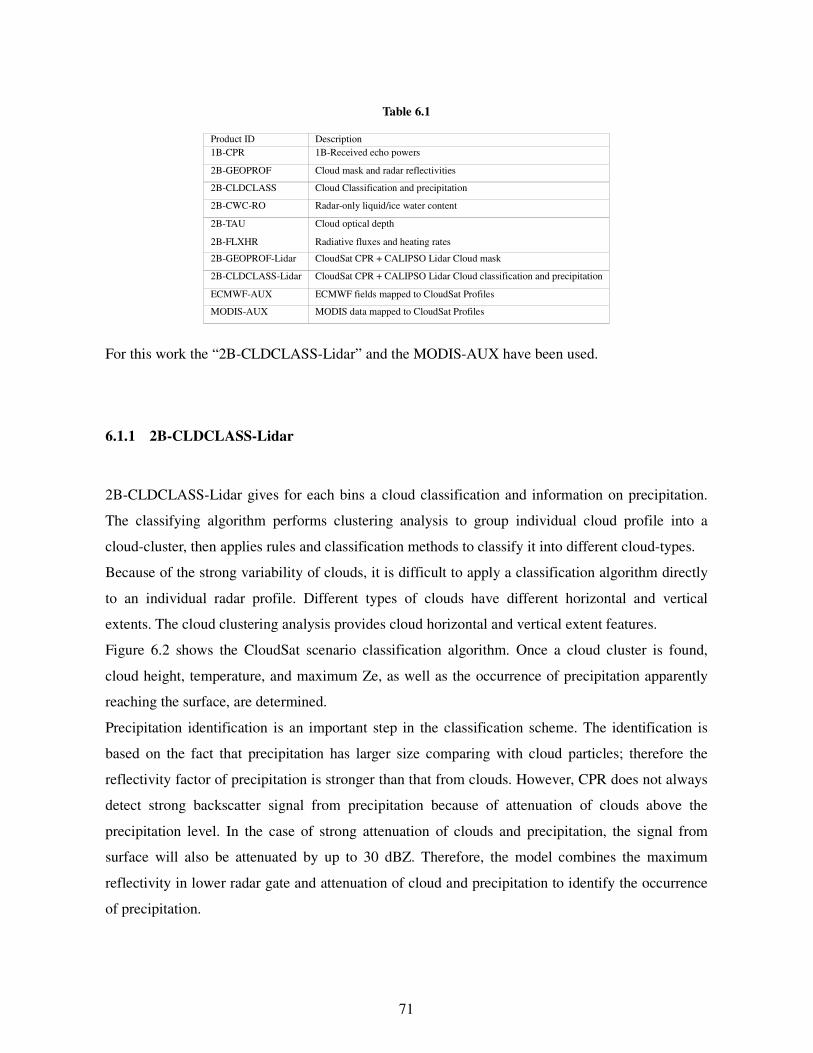
71
Table 6.1
Product ID Description
1B-CPR 1B-Received echo powers
2B-GEOPROF Cloud mask and radar reflectivities
2B-CLDCLASS Cloud Classification and precipitation
2B-CWC-RO Radar-only liquid/ice water content
2B-TAU Cloud optical depth
2B-FLXHR Radiative fluxes and heating rates
2B-GEOPROF-Lidar CloudSat CPR + CALIPSO Lidar Cloud mask
2B-CLDCLASS-Lidar CloudSat CPR + CALIPSO Lidar Cloud classification and precipitation
ECMWF-AUX ECMWF fields mapped to CloudSat Profiles
MODIS-AUX MODIS data mapped to CloudSat Profiles
For this work the “2B-CLDCLASS-Lidar” and the MODIS-AUX have been used.
6.1.1 2B-CLDCLASS-Lidar
2B-CLDCLASS-Lidar gives for each bins a cloud classification and information on precipitation.
The classifying algorithm performs clustering analysis to group individual cloud profile into a
cloud-cluster, then applies rules and classification methods to classify it into different cloud-types.
Because of the strong variability of clouds, it is difficult to apply a classification algorithm directly
to an individual radar profile. Different types of clouds have different horizontal and vertical
extents. The cloud clustering analysis provides cloud horizontal and vertical extent features.
Figure 6.2 shows the CloudSat scenario classification algorithm. Once a cloud cluster is found,
cloud height, temperature, and maximum Ze, as well as the occurrence of precipitation apparently
reaching the surface, are determined.
Precipitation identification is an important step in the classification scheme. The identification is
based on the fact that precipitation has larger size comparing with cloud particles; therefore the
reflectivity factor of precipitation is stronger than that from clouds. However, CPR does not always
detect strong backscatter signal from precipitation because of attenuation of clouds above the
precipitation level. In the case of strong attenuation of clouds and precipitation, the signal from
surface will also be attenuated by up to 30 dBZ. Therefore, the model combines the maximum
reflectivity in lower radar gate and attenuation of cloud and precipitation to identify the occurrence
of precipitation.
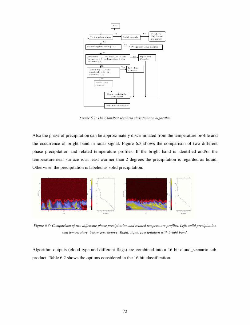
72
Figure 6.2: The CloudSat scenario classification algorithm
Also the phase of precipitation can be approximately discriminated from the temperature profile and
the occurrence of bright band in radar signal. Figure 6.3 shows the comparison of two different
phase precipitation and related temperature profiles. If the bright band is identified and/or the
temperature near surface is at least warmer than 2 degrees the precipitation is regarded as liquid.
Otherwise, the precipitation is labeled as solid precipitation.
Figure 6.3: Comparison of two differente phase precipitation and related temperature profiles. Left: solid precipitation
and temperature below zero degree; Right: liquid precipitation with bright band.
Algorithm outputs (cloud type and different flags) are combined into a 16 bit cloud_scenario sub-
product. Table 6.2 shows the options considered in the 16 bit classification.
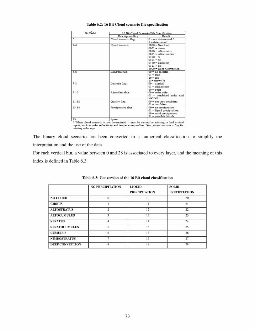
73
Table 6.2: 16 Bit Cloud scenario file specification
The binary cloud scenario has been converted in a numerical classification to simplify the
interpretation and the use of the data.
For each vertical bin, a value between 0 and 28 is associated to every layer, and the meaning of this
index is defined in Table 6.3.
Table 6.3: Conversion of the 16 Bit cloud classification
NO PRECIPITATION LIQUID
PRECIPITATION
SOLID
PRECIPITATION
NO CLOUD 0 10 20
CIRRUS 1 11 21
ALTOSTRATUS 2 12 22
ALTOCUMULUS 3 13 23
STRATUS 4 14 24
STRATOCUMULUS 5 15 25
CUMULUS 6 16 26
NIMBOSTRATUS 7 17 27
DEEP CONVECTION 8 18 28
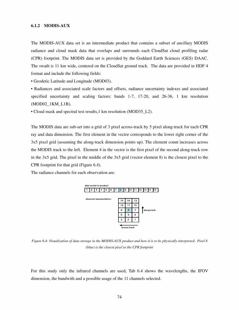
74
6.1.2 MODIS-AUX
The MODIS-AUX data set is an intermediate product that contains a subset of ancillary MODIS
radiance and cloud mask data that overlaps and surrounds each CloudSat cloud profiling radar
(CPR) footprint. The MODIS data set is provided by the Goddard Earth Sciences (GES) DAAC.
The swath is 11 km wide, centered on the CloudSat ground track. The data are provided in HDF 4
format and include the following fields:
• Geodetic Latitude and Longitude (MOD03).
• Radiances and associated scale factors and offsets, radiance uncertainty indexes and associated
specified uncertainty and scaling factors: bands 1-7, 17-20, and 26-36, 1 km resolution
(MOD02_1KM_L1B).
• Cloud mask and spectral test results,1 km resolution (MOD35_L2).
The MODIS data are sub-set into a grid of 3 pixel across-track by 5 pixel along-track for each CPR
ray and data dimension. The first element in the vector corresponds to the lower right corner of the
3x5 pixel grid (assuming the along-track dimension points up). The element count increases across
the MODIS track to the left. Element 4 in the vector is the first pixel of the second along-track row
in the 3x5 grid. The pixel in the middle of the 3x5 grid (vector element 8) is the closest pixel to the
CPR footprint for that grid (Figure 6.4).
The radiance channels for each observation are:
Figure 6.4: Visualization of data storage in the MODIS-AUX product and how it is to be physically interpreted. Pixel 8
(blue) is the closest pixel to the CPR footprint
For this study only the infrared channels are used, Tab 6.4 shows the wavelengths, the IFOV
dimension, the bandwith and a possible usage of the 11 channels selected.
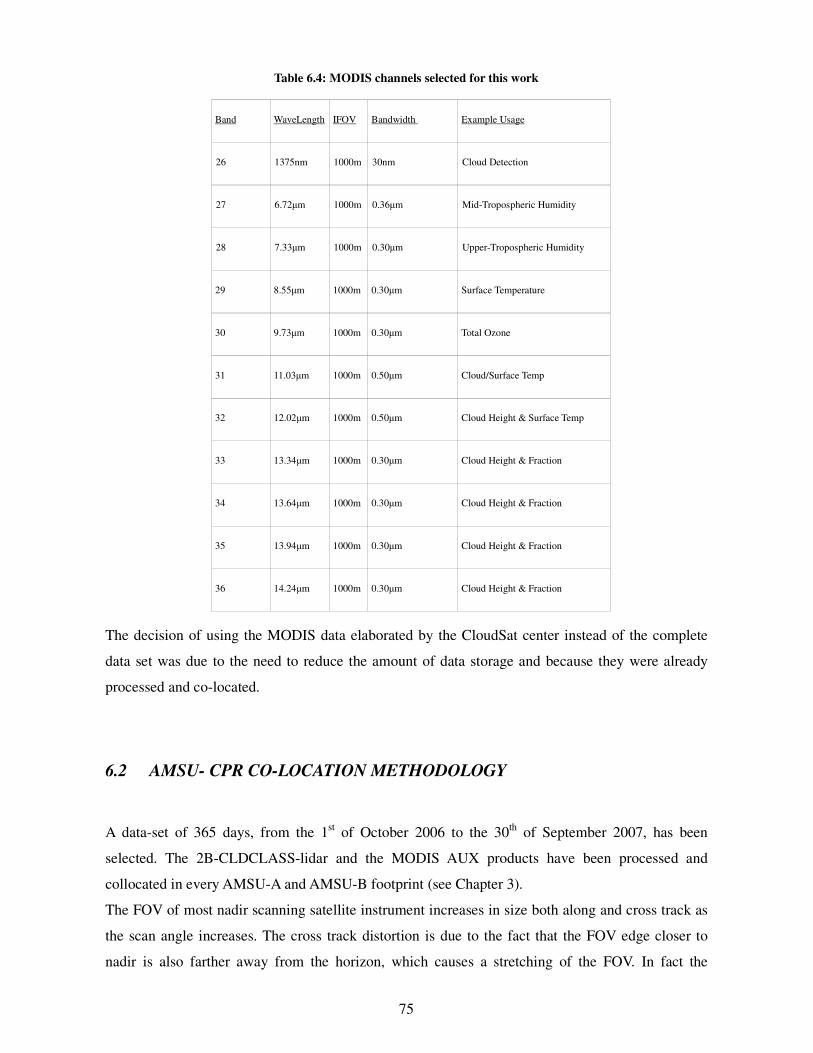
75
Table 6.4: MODIS channels selected for this work
Band WaveLength IFOV Bandwidth Example Usage
26 1375nm 1000m 30nm Cloud Detection
27 6.72µm 1000m 0.36µm Mid-Tropospheric Humidity
28 7.33µm 1000m 0.30µm Upper-Tropospheric Humidity
29 8.55µm 1000m 0.30µm Surface Temperature
30 9.73µm 1000m 0.30µm Total Ozone
31 11.03µm 1000m 0.50µm Cloud/Surface Temp
32 12.02µm 1000m 0.50µm Cloud Height & Surface Temp
33 13.34µm 1000m 0.30µm Cloud Height & Fraction
34 13.64µm 1000m 0.30µm Cloud Height & Fraction
35 13.94µm 1000m 0.30µm Cloud Height & Fraction
36 14.24µm 1000m 0.30µm Cloud Height & Fraction
The decision of using the MODIS data elaborated by the CloudSat center instead of the complete
data set was due to the need to reduce the amount of data storage and because they were already
processed and co-located.
6.2 AMSU- CPR CO-LOCATION METHODOLOGY
A data-set of 365 days, from the 1st of October 2006 to the 30
th of September 2007, has been
selected. The 2B-CLDCLASS-lidar and the MODIS AUX products have been processed and
collocated in every AMSU-A and AMSU-B footprint (see Chapter 3).
The FOV of most nadir scanning satellite instrument increases in size both along and cross track as
the scan angle increases. The cross track distortion is due to the fact that the FOV edge closer to
nadir is also farther away from the horizon, which causes a stretching of the FOV. In fact the
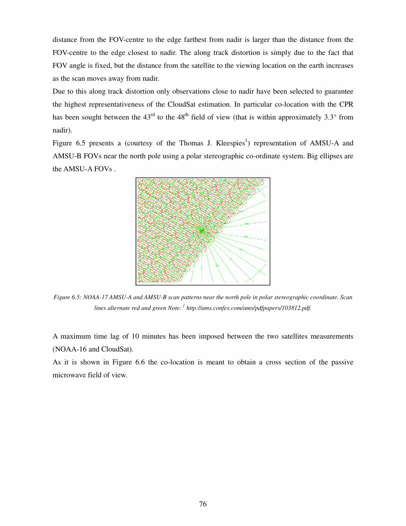
76
distance from the FOV-centre to the edge farthest from nadir is larger than the distance from the
FOV-centre to the edge closest to nadir. The along track distortion is simply due to the fact that
FOV angle is fixed, but the distance from the satellite to the viewing location on the earth increases
as the scan moves away from nadir.
Due to this along track distortion only observations close to nadir have been selected to guarantee
the highest representativeness of the CloudSat estimation. In particular co-location with the CPR
has been sought between the 43rd
to the 48th
field of view (that is within approximately 3.3° from
nadir).
Figure 6.5 presents a (courtesy of the Thomas J. Kleespies1) representation of AMSU-A and
AMSU-B FOVs near the north pole using a polar stereographic co-ordinate system. Big ellipses are
the AMSU-A FOVs .
Figure 6.5: NOAA-17 AMSU-A and AMSU-B scan patterns near the north pole in polar stereographic coordinate. Scan
lines alternate red and green Note: 1
http://ams.confex.com/ams/pdfpapers/103812.pdf.
A maximum time lag of 10 minutes has been imposed between the two satellites measurements
(NOAA-16 and CloudSat).
As it is shown in Figure 6.6 the co-location is meant to obtain a cross section of the passive
microwave field of view.
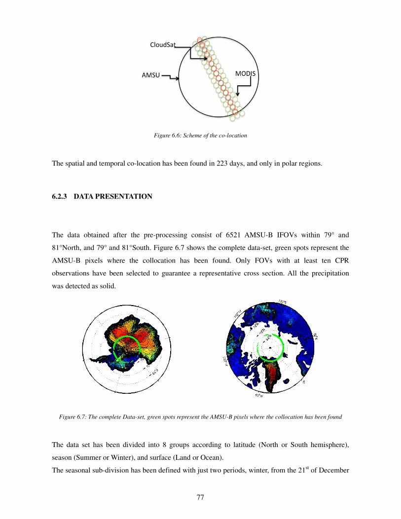
77
Figure 6.6: Scheme of the co-location
The spatial and temporal co-location has been found in 223 days, and only in polar regions.
6.2.3 DATA PRESENTATION
The data obtained after the pre-processing consist of 6521 AMSU-B IFOVs within 79° and
81°North, and 79° and 81°South. Figure 6.7 shows the complete data-set, green spots represent the
AMSU-B pixels where the collocation has been found. Only FOVs with at least ten CPR
observations have been selected to guarantee a representative cross section. All the precipitation
was detected as solid.
Figure 6.7: The complete Data-set, green spots represent the AMSU-B pixels where the collocation has been found
The data set has been divided into 8 groups according to latitude (North or South hemisphere),
season (Summer or Winter), and surface (Land or Ocean).
The seasonal sub-division has been defined with just two periods, winter, from the 21st of December
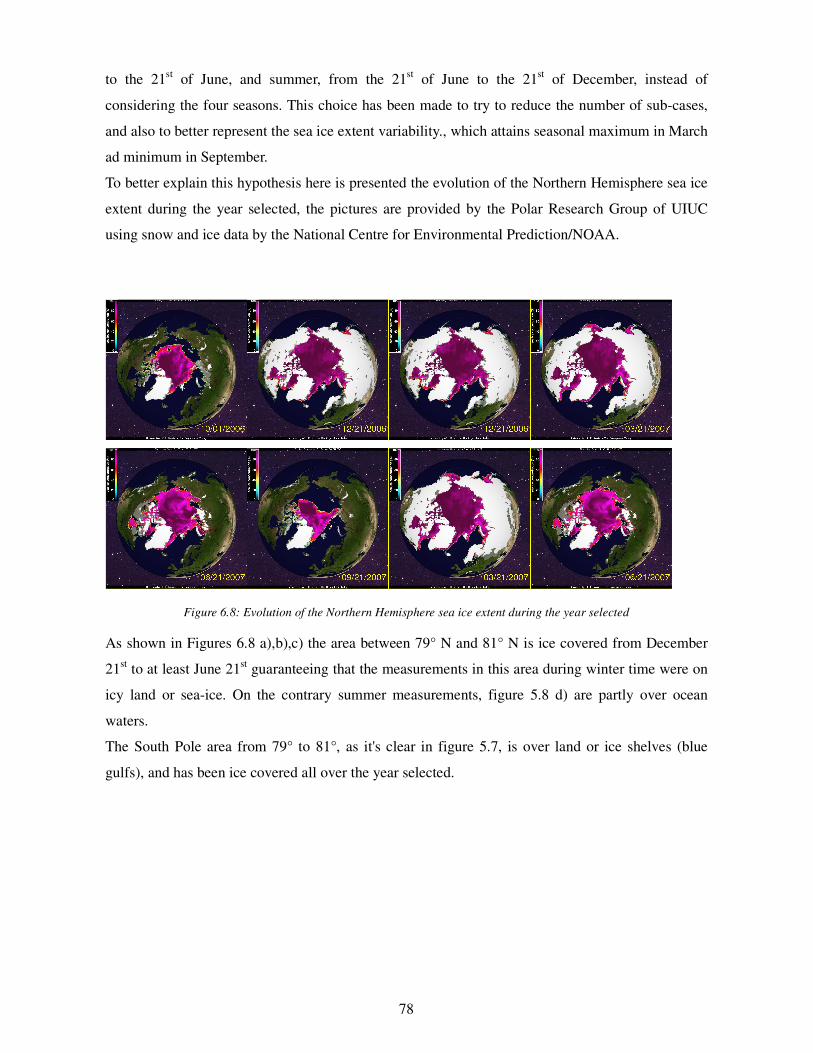
78
to the 21st of June, and summer, from the 21
st of June to the 21
st of December, instead of
considering the four seasons. This choice has been made to try to reduce the number of sub-cases,
and also to better represent the sea ice extent variability., which attains seasonal maximum in March
ad minimum in September.
To better explain this hypothesis here is presented the evolution of the Northern Hemisphere sea ice
extent during the year selected, the pictures are provided by the Polar Research Group of UIUC
using snow and ice data by the National Centre for Environmental Prediction/NOAA.
Figure 6.8: Evolution of the Northern Hemisphere sea ice extent during the year selected
As shown in Figures 6.8 a),b),c) the area between 79° N and 81° N is ice covered from December
21st to at least June 21
st guaranteeing that the measurements in this area during winter time were on
icy land or sea-ice. On the contrary summer measurements, figure 5.8 d) are partly over ocean
waters.
The South Pole area from 79° to 81°, as it's clear in figure 5.7, is over land or ice shelves (blue
gulfs), and has been ice covered all over the year selected.
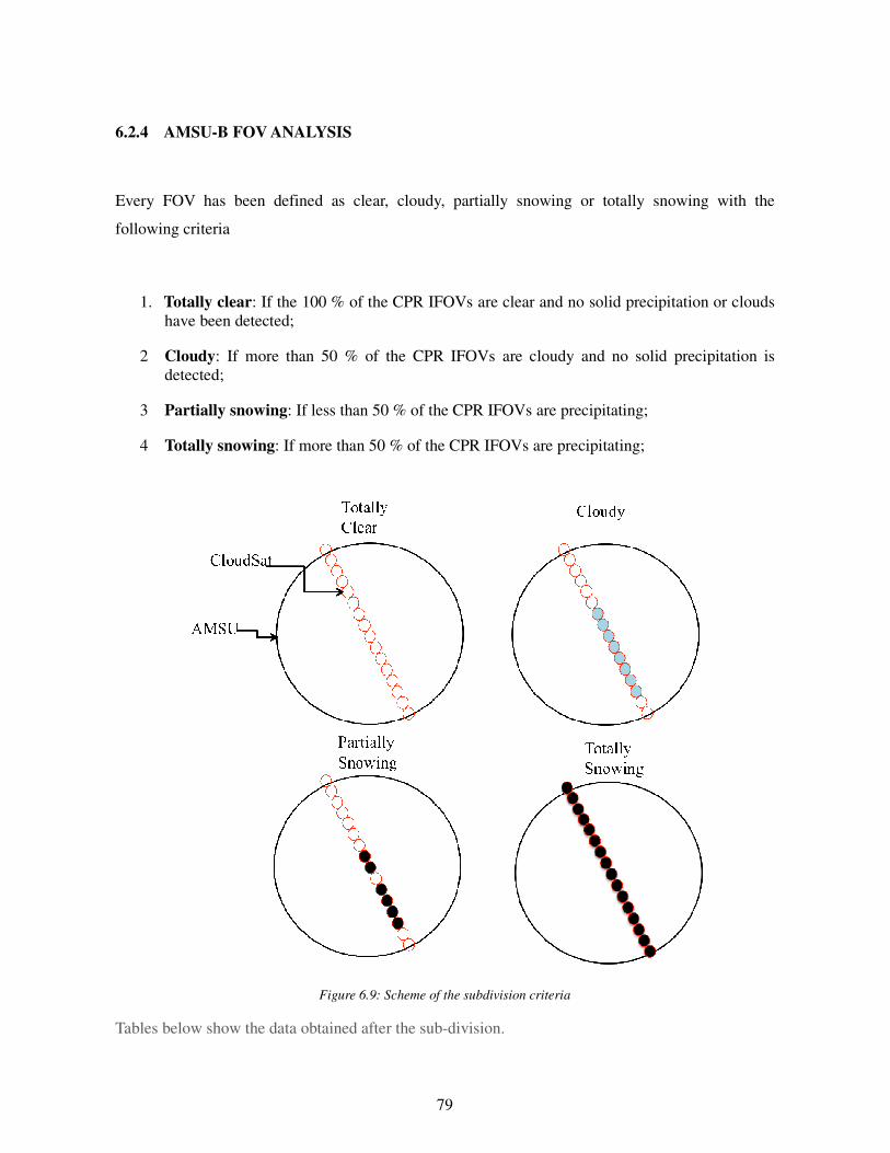
79
6.2.4 AMSU-B FOV ANALYSIS
Every FOV has been defined as clear, cloudy, partially snowing or totally snowing with the
following criteria
1. Totally clear: If the 100 % of the CPR IFOVs are clear and no solid precipitation or clouds
have been detected;
2 Cloudy: If more than 50 % of the CPR IFOVs are cloudy and no solid precipitation is
detected;
3 Partially snowing: If less than 50 % of the CPR IFOVs are precipitating;
4 Totally snowing: If more than 50 % of the CPR IFOVs are precipitating;
Figure 6.9: Scheme of the subdivision criteria
Tables below show the data obtained after the sub-division.
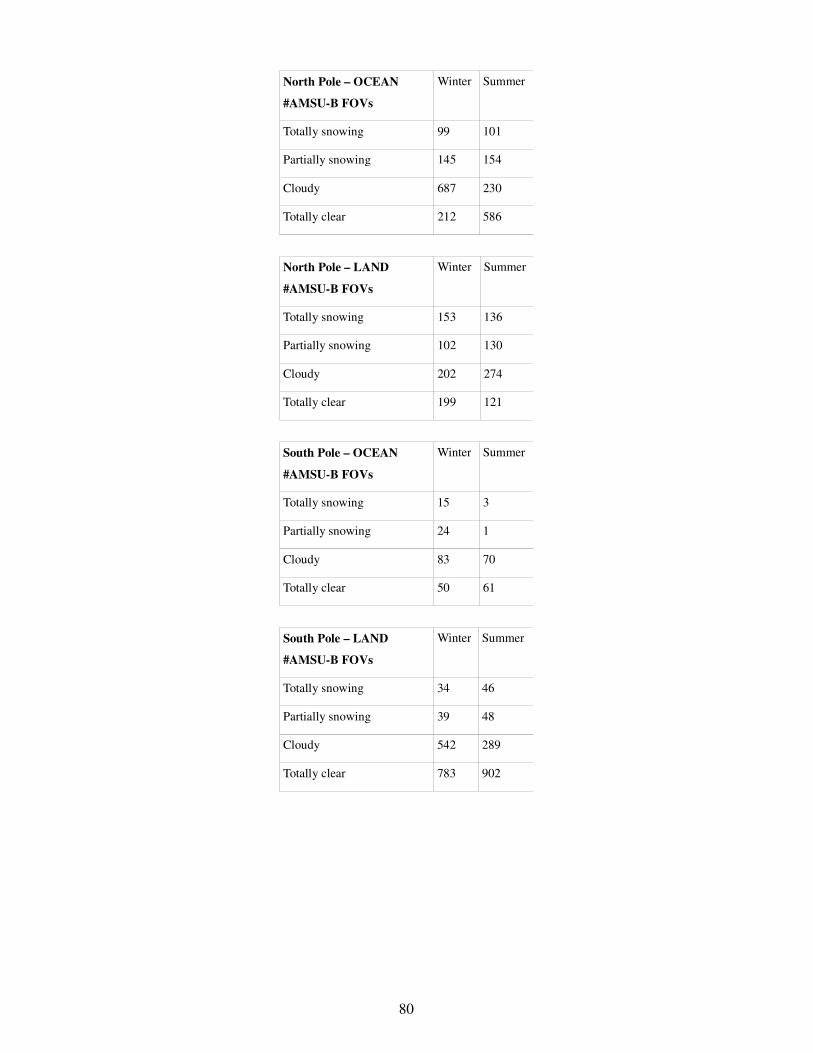
80
North Pole – OCEAN
#AMSU-B FOVs
Winter Summer
Totally snowing 99 101
Partially snowing 145 154
Cloudy 687 230
Totally clear 212 586
North Pole – LAND
#AMSU-B FOVs
Winter Summer
Totally snowing 153 136
Partially snowing 102 130
Cloudy 202 274
Totally clear 199 121
South Pole – OCEAN
#AMSU-B FOVs
Winter Summer
Totally snowing 15 3
Partially snowing 24 1
Cloudy 83 70
Totally clear 50 61
South Pole – LAND
#AMSU-B FOVs
Winter Summer
Totally snowing 34 46
Partially snowing 39 48
Cloudy 542 289
Totally clear 783 902
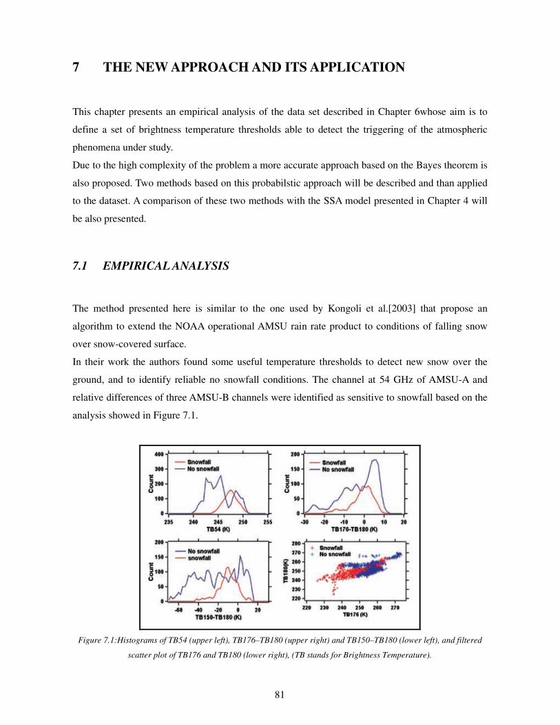
81
7 THE NEW APPROACH AND ITS APPLICATION
This chapter presents an empirical analysis of the data set described in Chapter 6whose aim is to
define a set of brightness temperature thresholds able to detect the triggering of the atmospheric
phenomena under study.
Due to the high complexity of the problem a more accurate approach based on the Bayes theorem is
also proposed. Two methods based on this probabilstic approach will be described and than applied
to the dataset. A comparison of these two methods with the SSA model presented in Chapter 4 will
be also presented.
7.1 EMPIRICAL ANALYSIS
The method presented here is similar to the one used by Kongoli et al.[2003] that propose an
algorithm to extend the NOAA operational AMSU rain rate product to conditions of falling snow
over snow-covered surface.
In their work the authors found some useful temperature thresholds to detect new snow over the
ground, and to identify reliable no snowfall conditions. The channel at 54 GHz of AMSU-A and
relative differences of three AMSU-B channels were identified as sensitive to snowfall based on the
analysis showed in Figure 7.1.
Figure 7.1:Histograms of TB54 (upper left), TB176–TB180 (upper right) and TB150–TB180 (lower left), and filtered
scatter plot of TB176 and TB180 (lower right), (TB stands for Brightness Temperature).
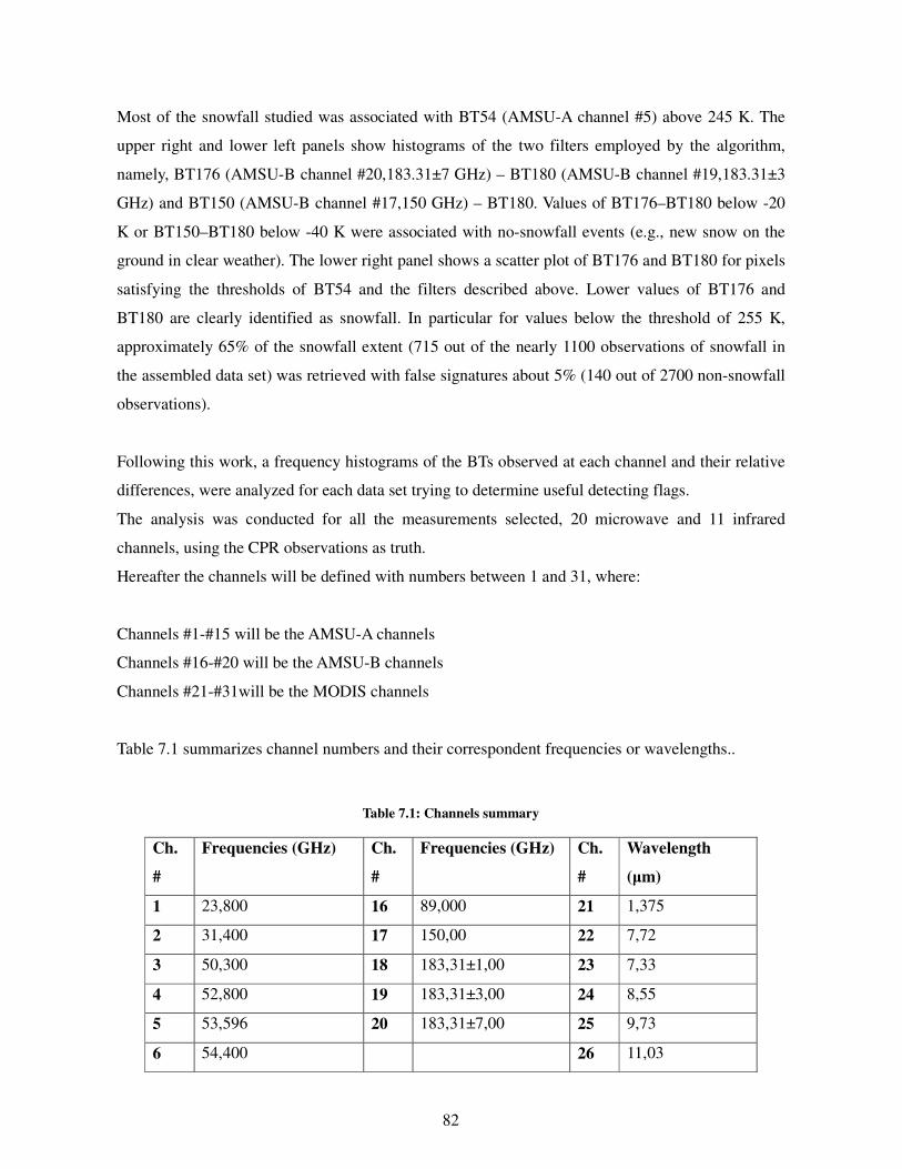
82
Most of the snowfall studied was associated with BT54 (AMSU-A channel #5) above 245 K. The
upper right and lower left panels show histograms of the two filters employed by the algorithm,
namely, BT176 (AMSU-B channel #20,183.31±7 GHz) – BT180 (AMSU-B channel #19,183.31±3
GHz) and BT150 (AMSU-B channel #17,150 GHz) – BT180. Values of BT176–BT180 below -20
K or BT150–BT180 below -40 K were associated with no-snowfall events (e.g., new snow on the
ground in clear weather). The lower right panel shows a scatter plot of BT176 and BT180 for pixels
satisfying the thresholds of BT54 and the filters described above. Lower values of BT176 and
BT180 are clearly identified as snowfall. In particular for values below the threshold of 255 K,
approximately 65% of the snowfall extent (715 out of the nearly 1100 observations of snowfall in
the assembled data set) was retrieved with false signatures about 5% (140 out of 2700 non-snowfall
observations).
Following this work, a frequency histograms of the BTs observed at each channel and their relative
differences, were analyzed for each data set trying to determine useful detecting flags.
The analysis was conducted for all the measurements selected, 20 microwave and 11 infrared
channels, using the CPR observations as truth.
Hereafter the channels will be defined with numbers between 1 and 31, where:
Channels #1-#15 will be the AMSU-A channels
Channels #16-#20 will be the AMSU-B channels
Channels #21-#31will be the MODIS channels
Table 7.1 summarizes channel numbers and their correspondent frequencies or wavelengths..
Table 7.1: Channels summary
Ch.
#
Frequencies (GHz) Ch.
#
Frequencies (GHz) Ch.
#
Wavelength
(µm)
1 23,800 16 89,000 21 1,375
2 31,400 17 150,00 22 7,72
3 50,300 18 183,31±1,00 23 7,33
4 52,800 19 183,31±3,00 24 8,55
5 53,596 20 183,31±7,00 25 9,73
6 54,400 26 11,03

83
7 54,940 27 12,02
8 55,500 28 13,34
9 f0=57,290 29 13,64
10 f0±0,217 30 13,94
11 f0±0,3222±0,048 31 14,24
12 f0±0,3222±0,022
13 f0±0,3222±0,010
14 f0±0,322.2±0,0045
15 89,000
To find the best flag an algorithm that evaluates the percentages of totally clear, cloudy, partially
and totally snowing was applied to each channel and to their relative differences.
For every single case selected, an optimum value, which maximises the sum of the clear and cloudy
percentage minus the sum of the partially and the totally snowing, was found.
The best results are here presented for each sub-set:
1. South Pole Winter over Land (SWL)
2. South Pole Winter over Ocean (SWO)
3. South Pole Summer over Land (SSL)
4. South Pole Summer over Ocean (SSO)
5. North Pole Winter over Land (NWL)
6. North Pole Winter over Ocean (NWO)
7. North Pole Summer over Land (NSL)
8. North Pole Summer over Ocean (NSO)
For each case a table sets in evidence the most sensitive channels, showing the percentage of
detection and the brightness temperature threshold. All the percentage presented are evaluated
computing for each of the four classified group, the number of FOVS below the threshold divided
by their total number.
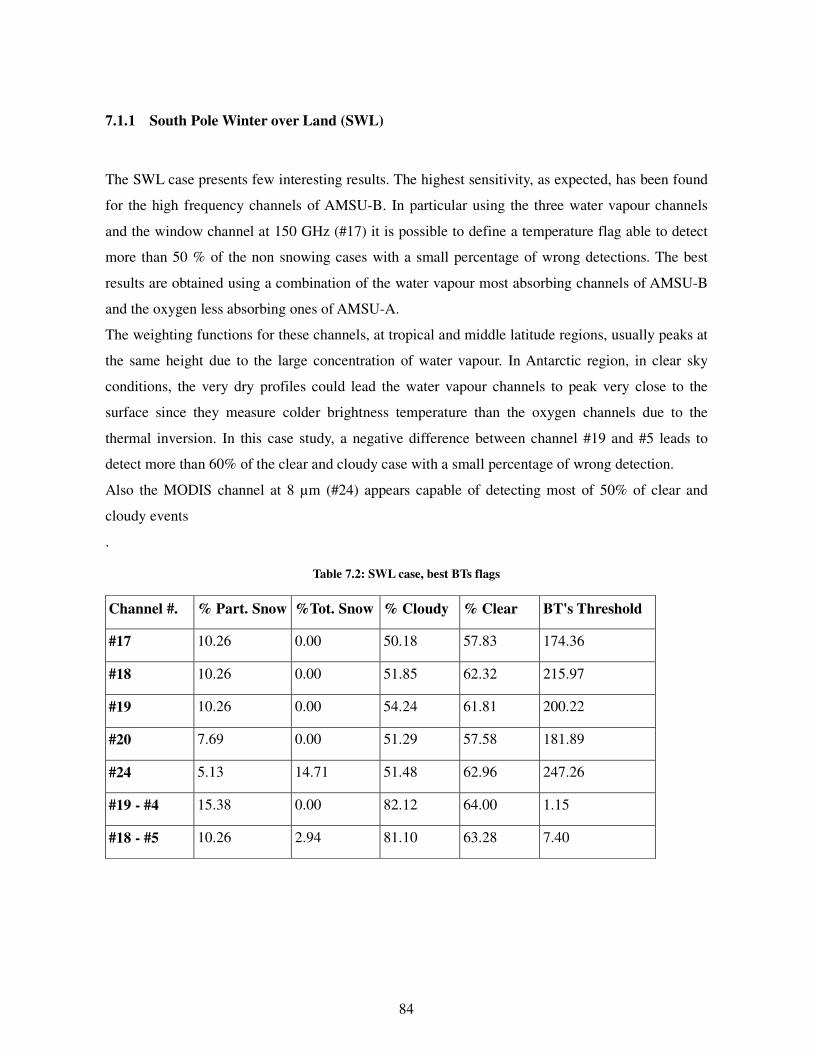
84
7.1.1 South Pole Winter over Land (SWL)
The SWL case presents few interesting results. The highest sensitivity, as expected, has been found
for the high frequency channels of AMSU-B. In particular using the three water vapour channels
and the window channel at 150 GHz (#17) it is possible to define a temperature flag able to detect
more than 50 % of the non snowing cases with a small percentage of wrong detections. The best
results are obtained using a combination of the water vapour most absorbing channels of AMSU-B
and the oxygen less absorbing ones of AMSU-A.
The weighting functions for these channels, at tropical and middle latitude regions, usually peaks at
the same height due to the large concentration of water vapour. In Antarctic region, in clear sky
conditions, the very dry profiles could lead the water vapour channels to peak very close to the
surface since they measure colder brightness temperature than the oxygen channels due to the
thermal inversion. In this case study, a negative difference between channel #19 and #5 leads to
detect more than 60% of the clear and cloudy case with a small percentage of wrong detection.
Also the MODIS channel at 8 µm (#24) appears capable of detecting most of 50% of clear and
cloudy events
.
Table 7.2: SWL case, best BTs flags
Channel #. % Part. Snow %Tot. Snow % Cloudy % Clear BT's Threshold
#17 10.26 0.00 50.18 57.83 174.36
#18 10.26 0.00 51.85 62.32 215.97
#19 10.26 0.00 54.24 61.81 200.22
#20 7.69 0.00 51.29 57.58 181.89
#24 5.13 14.71 51.48 62.96 247.26
#19 - #4 15.38 0.00 82.12 64.00 1.15
#18 - #5 10.26 2.94 81.10 63.28 7.40
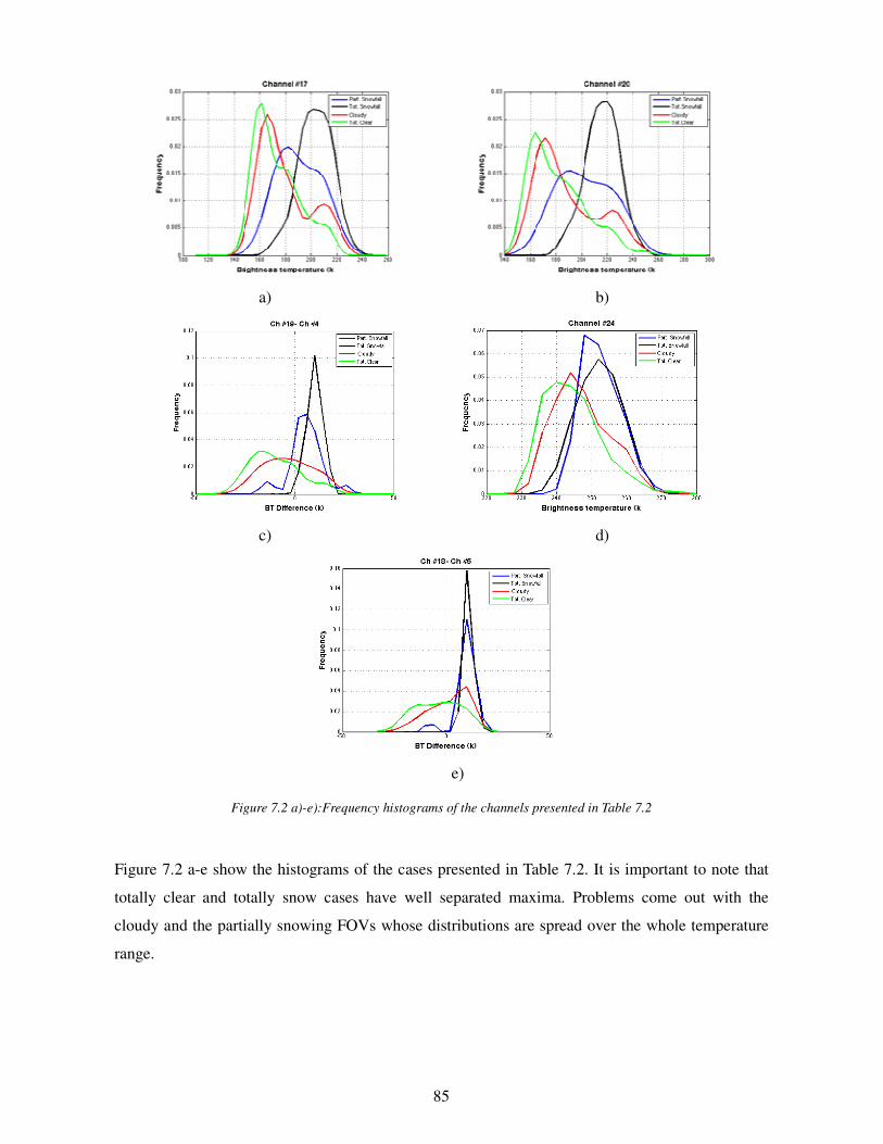
85
a) b)
c) d)
e)
Figure 7.2 a)-e):Frequency histograms of the channels presented in Table 7.2
Figure 7.2 a-e show the histograms of the cases presented in Table 7.2. It is important to note that
totally clear and totally snow cases have well separated maxima. Problems come out with the
cloudy and the partially snowing FOVs whose distributions are spread over the whole temperature
range.
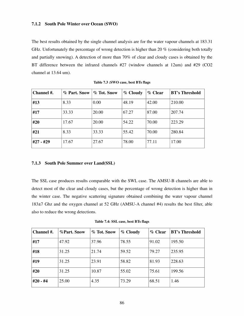
86
7.1.2 South Pole Winter over Ocean (SWO)
The best results obtained by the single channel analysis are for the water vapour channels at 183.31
GHz. Unfortunately the percentage of wrong detection is higher than 20 % (considering both totally
and partially snowing). A detection of more than 70% of clear and cloudy cases is obtained by the
BT difference between the infrared channels #27 (window channels at 12um) and #29 (CO2
channel at 13.64 um).
Table 7.3 :SWO case, best BTs flags
Channel #. % Part. Snow % Tot. Snow % Cloudy % Clear BT's Threshold
#13 8.33 0.00 48.19 42.00 210.00
#17 33.33 20.00 67.27 87.00 207.74
#20 17.67 20.00 54.22 70.00 223.29
#21 8.33 33.33 55.42 70.00 280.84
#27 - #29 17.67 27.67 78.00 77.11 17.00
7.1.3 South Pole Summer over Land(SSL)
The SSL case produces results comparable with the SWL case. The AMSU-B channels are able to
detect most of the clear and cloudy cases, but the percentage of wrong detection is higher than in
the winter case. The negative scattering signature obtained combining the water vapour channel
183±7 Ghz and the oxygen channel at 52 GHz (AMSU-A channel #4) results the best filter, able
also to reduce the wrong detections.
Table 7.4: SSL case, best BTs flags
Channel #. %Part. Snow % Tot. Snow % Cloudy % Clear BT's Threshold
#17 47.92 37.96 78.55 91.02 195.50
#18 31.25 21.74 59.52 79.27 235.95
#19 31.25 23.91 58.82 81.93 228.63
#20 31.25 10.87 55.02 75.61 199.56
#20 - #4 25.00 4.35 73.29 68.51 1.46
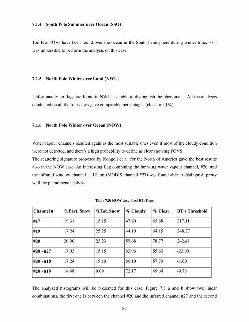
87
7.1.4 South Pole Summer over Ocean (SSO)
Too few FOVs have been found over the ocean in the South hemisphere during winter time, so it
was impossible to perform the analysis on this case.
7.1.5 North Pole Winter over Land (NWL)
Unfortunately no flags are found in NWL case able to distinguish the phenomena. All the analyses
conducted on all the four cases gave comparable percentages (close to 50 %).
7.1.6 North Pole Winter over Ocean (NOW)
Water vapour channels resulted again as the most suitable ones even if most of the cloudy condition
were not detected, and there's a high probability to define as clear snowing FOVS.
The scattering signature proposed by Kongoli et al. for the North of America gave the best results
also in the NOW case. An interesting flag combining the far wing water vapour channel, #20, and
the infrared window channel at 12 µm (MODIS channel #27) was found able to distinguish pretty
well the phenomena analyzed.
Table 7.5: NOW case, best BTs flags
Channel #. %Part. Snow %Tot. Snow % Cloudy % Clear BT's Threshold
#17 19.31 15.15 47.60 63.68 217.11
#19 17.24 25.25 44.10 64.15 248.27
#20 20.00 23.23 59.68 78.77 242.41
#20 - #27 17.93 15.15 83.96 55.60 -23.99
#20 - #18 17.24 19.19 80.19 57.79 -1.00
#20 - #19 14.48 9.09 72.17 49.64 -9.78
The analyzed histograms will be presented for this case. Figure 7.3 a and b show two linear
combinations, the first one is between the channel #20 and the infrared channel #27 and the second
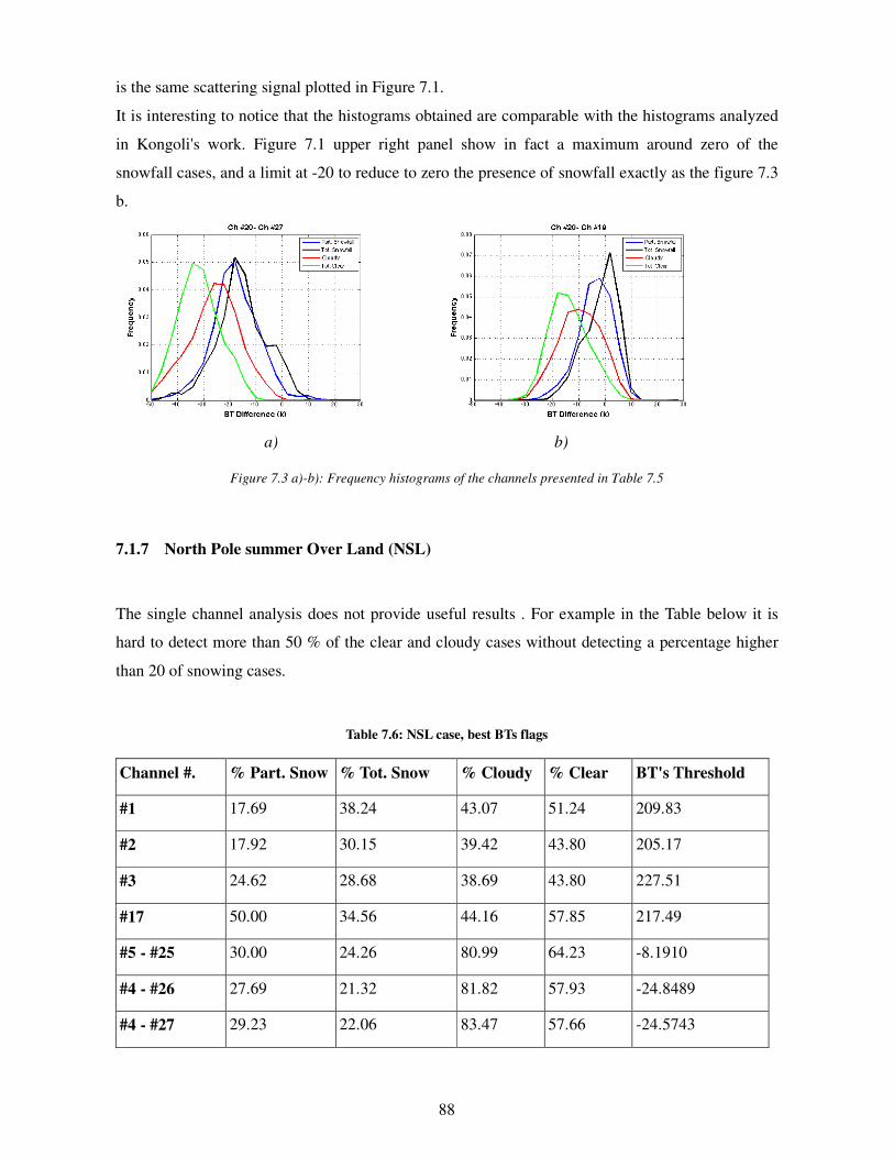
88
is the same scattering signal plotted in Figure 7.1.
It is interesting to notice that the histograms obtained are comparable with the histograms analyzed
in Kongoli's work. Figure 7.1 upper right panel show in fact a maximum around zero of the
snowfall cases, and a limit at -20 to reduce to zero the presence of snowfall exactly as the figure 7.3
b.
a) b)
Figure 7.3 a)-b): Frequency histograms of the channels presented in Table 7.5
7.1.7 North Pole summer Over Land (NSL)
The single channel analysis does not provide useful results . For example in the Table below it is
hard to detect more than 50 % of the clear and cloudy cases without detecting a percentage higher
than 20 of snowing cases.
Table 7.6: NSL case, best BTs flags
Channel #. % Part. Snow % Tot. Snow % Cloudy % Clear BT's Threshold
#1 17.69 38.24 43.07 51.24 209.83
#2 17.92 30.15 39.42 43.80 205.17
#3 24.62 28.68 38.69 43.80 227.51
#17 50.00 34.56 44.16 57.85 217.49
#5 - #25 30.00 24.26 80.99 64.23 -8.1910
#4 - #26 27.69 21.32 81.82 57.93 -24.8489
#4 - #27 29.23 22.06 83.47 57.66 -24.5743
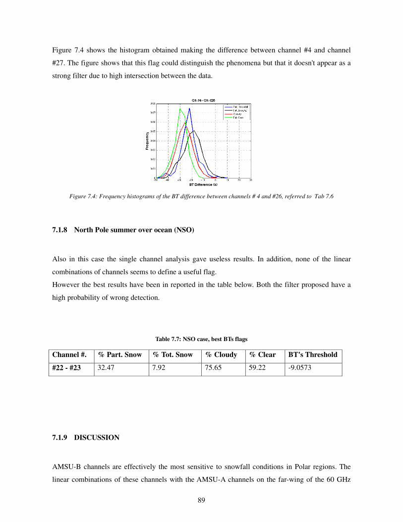
89
Figure 7.4 shows the histogram obtained making the difference between channel #4 and channel
#27. The figure shows that this flag could distinguish the phenomena but that it doesn't appear as a
strong filter due to high intersection between the data.
Figure 7.4: Frequency histograms of the BT difference between channels # 4 and #26, referred to Tab 7.6
7.1.8 North Pole summer over ocean (NSO)
Also in this case the single channel analysis gave useless results. In addition, none of the linear
combinations of channels seems to define a useful flag.
However the best results have been in reported in the table below. Both the filter proposed have a
high probability of wrong detection.
Table 7.7: NSO case, best BTs flags
Channel #. % Part. Snow % Tot. Snow % Cloudy % Clear BT's Threshold
#22 - #23 32.47 7.92 75.65 59.22 -9.0573
7.1.9 DISCUSSION
AMSU-B channels are effectively the most sensitive to snowfall conditions in Polar regions. The
linear combinations of these channels with the AMSU-A channels on the far-wing of the 60 GHz
90
line, allow to detect snowfall over Antarctic with a percentage of wrong detection smaller than 30%.
Few channel linear combinations are found efficient for the Arctic region over the ocean, where the
best results are obtained using the brightness temperature differences between the water vapour
channels around 183 GHz.
In the North hemisphere cases, in particular in summer, the linear combinations of infrared window
and microwave oxygen channels appear capable to distinguish more than 70% of the clear and
cloudy cases, with a percentage of wrong detection close to 30%.
The results obtained, even if encouraging, are still far from the definition of a unique method to
combine the observations in order to evaluate a probability of detection.
The empirical analysis gives the opportunity to identify possible flags but it is not an efficient
method to find the most significative channel combination.
In order to solve this problem a statistical approach based on the Bayes theorem will be proposed in
the next paragraphs.
7.2 COMBINING DIFFERENT MEASUREMENTS AND MODELS IN
ORDER TO IMPROVE PREDICTABILITY
Prior to discussing predictability, it is necessary to clarify the distinction between
“prediction”, which is the action which allows to estimate an unknown quantity at time t, the
“predictand”, knowing other quantities up to time t, the “predictors”, from the “forecast”, which is
the action which allows to estimate an unknown quantity, that can still be called “predictand”, at
time t+k∆t into the future knowing other quantities, the “predictors”, up to time t.
In any case, the scope of prediction or of forecast is the reduction of the uncertainty on the
estimation of an unknown quantity.
In order to assess this uncertainty, generally referred to as the “predictive uncertainty”, or as
“forecasting uncertainty” one generally starts from his prior knowledge. For instance, one may use
the climatological distribution of snow occurrence to describe his prior belief on the possibility of
snow. In general, this a-priori probability density function is very flat and is not sufficiently dense
around some specific value to allow for a safe decision, as for instance on whether it will snow or
not.
Therefore it is necessary to gather additional information, such as additional measurements or
results from one or more models. There is no substantial difference between a measurement or a
modelled quantity apart from the type of errors affecting them.
91
Measurements can be quite accurate and are affected by measurement errors, but if these
measurements are not direct measures of the “predictand”, thus similar to “model predictions”, they
become “predictors” of the “predictand”, which implies the addition of a modelling error; modelled
quantities do in fact incorporate both measurement errors and model errors, which can be large if
the model is not very accurate. Nonetheless models become essential when dealing with
“forecasting”, because at any future time no measurement are available, and one can only use
modelled quantities in order to increase insight into the future.
Given that, apart from the time of issue, there is no substantial difference between “prediction” or
“forecast” when the measurements and/or the modelled quantities are available, because the
problem is always to assess the uncertainty of a predictand given one or more predictors, only the
term “prediction” will be used in the sequel for the sake of clarity.
The prediction problem can be tackled with two different approaches, depending on the nature of
the decision problem to be solved. The first approach relates to continuous processes, which require
the estimation of the entire predictive probability function: for instance when dealing with flood
damages, which vary with the water level reached, the expected value of these damages can only be
estimated if the full probability density of water levels is available. There are other cases where
only the integral above or below a threshold of the predictive density is needed. This is the case for
instance when one has to decide whether it snows or it doesn’t on the basis of one or more sensors
or models. All these cases, characterised by a threshold type of problem can be described in discrete
probability terms as will be discussed in the sequel.
7.2.1 Continuous Probability Problems: the Bayesian Model Averaging
Introduced by Raftery et al. [1993] Bayesian Model Averaging (BMA) has gained a certain
popularity in the latest years.
BMA aims at assessing the unconditional mean and variance of any value of the predictand on the
basis of several model predictions. Please note that the same concept can be extended to
measurements, with error descending from the measurement itself and the fact that the measured
quantity is not necessarily the one to be predicted.
Raftery et al. [2003] developed the approach on the assumption that the predictand as well as the
model predictions were approximately Normally distributed, while Vrugt and Robinson [2007]
relaxed this hypothesis and showed how to apply the BMA on Log-normal and Gamma distributed
variables.
92
In practice the Bayesian Inference problem, namely the need to estimate a posterior density for the
parameters) is overcome in the BMA by estimating a number of weights via a constrained
optimization problem:
( )1 1 1
1
ˆlog log
. . 1
j
S T K
w j j st jst
s= t= j=
K
j
j=
Max L = w p y | y
s t w =
∑∑ ∑
∑ (7.1)
where wj are the weights to be estimated, ( )jststj yyp ˆ is the conditional probability of sty , the
predictand at site s and time t , given jsty , model j unbiased prediction for sty , with S the
total number of observation sites, T the total number of observation time intervals and K the
number of used models.
It is worthwhile pointing out that the notation used by Raftery [2003], and Vrugt and Robinson
[2007], may lead to misunderstanding the real scope of BMA.
As previously stated, following the definition of predictive probability, BMA searches for an
“unconditional” predictive probability, by marginalising the effect of the different models using
their posterior probability.
Therefore, the following expression
( ) ( )∑=
=K
j
jjjK yypwyyyyp1
21ˆˆ,...,ˆ,ˆ
(7.2)
given as Eqn. (7.2) in Raftery et al [2003] and more or less identically reported in Eqn. 7 by Vrugt
and Robinson [2007], may be misleading, since it might appear that BMA aims at finding the
“conditional” predictive probability, which is the probability of observing the predictand y , given
all the different model predictions Kyyy ˆ,...,ˆ,ˆ21 .
A more convenient representation is that of Draper [1995]:
( ) ( )∑=
=K
j
jjj yypwyp1
ˆ,MD
(7.3)
where D is the ensemble of historical observations and M represents the ensemble of models.
This indicates that although the predictive density given in Eqn. (7.3) represents the “model
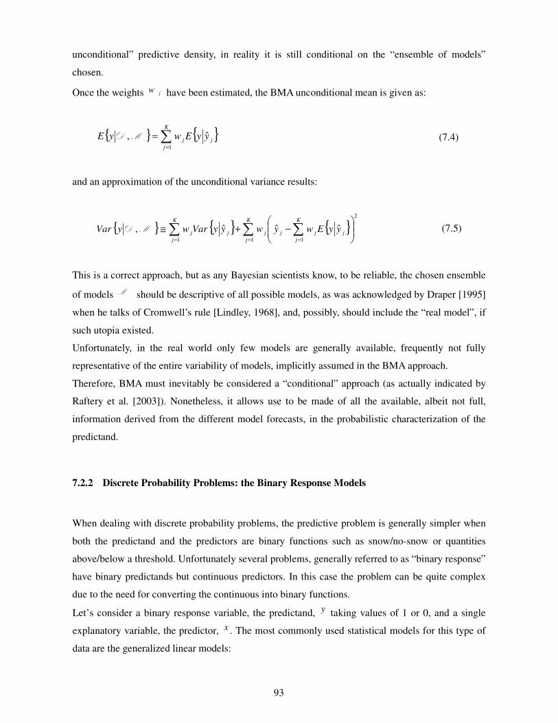
93
unconditional” predictive density, in reality it is still conditional on the “ensemble of models”
chosen.
Once the weights jw have been estimated, the BMA unconditional mean is given as:
{ } { }∑=
=K
j
jj yyEwyE1
ˆ,MD
(7.4)
and an approximation of the unconditional variance results:
{ } { } { }2
1 11
ˆˆˆ, ∑ ∑∑= ==
−+≅
K
j
K
j
jjjj
K
j
jj yyEwywyyVarwyVar MD
(7.5)
This is a correct approach, but as any Bayesian scientists know, to be reliable, the chosen ensemble
of models M should be descriptive of all possible models, as was acknowledged by Draper [1995]
when he talks of Cromwell’s rule [Lindley, 1968], and, possibly, should include the “real model”, if
such utopia existed.
Unfortunately, in the real world only few models are generally available, frequently not fully
representative of the entire variability of models, implicitly assumed in the BMA approach.
Therefore, BMA must inevitably be considered a “conditional” approach (as actually indicated by
Raftery et al. [2003]). Nonetheless, it allows use to be made of all the available, albeit not full,
information derived from the different model forecasts, in the probabilistic characterization of the
predictand.
7.2.2 Discrete Probability Problems: the Binary Response Models
When dealing with discrete probability problems, the predictive problem is generally simpler when
both the predictand and the predictors are binary functions such as snow/no-snow or quantities
above/below a threshold. Unfortunately several problems, generally referred to as “binary response”
have binary predictands but continuous predictors. In this case the problem can be quite complex
due to the need for converting the continuous into binary functions.
Let’s consider a binary response variable, the predictand, y taking values of 1 or 0, and a single
explanatory variable, the predictor, x . The most commonly used statistical models for this type of
data are the generalized linear models:
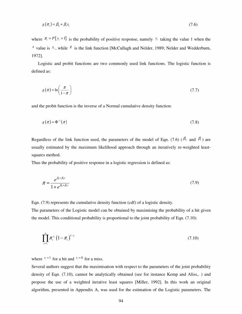
94
( ) 0 1π β β= +
i ig x
(7.6)
where { }1π = =i i
P y is the probability of positive response, namely iy taking the value 1 when the
x value is ix , while g is the link function [McCullagh and Nelder, 1989; Nelder and Wedderburn,
1972].
Logistic and probit functions are two commonly used link functions. The logistic function is
defined as:
( ) ln1
ππ
π
=
− g
(7.7)
and the probit function is the inverse of a Normal cumulative density function:
( ) ( )1π π−= Φg (7.8)
Regardless of the link function used, the parameters of the model of Eqn. (7.6) ( 0β and 1
β ) are
usually estimated by the maximum likelihood approach through an iteratively re-weighted least-
squares method.
Thus the probability of positive response in a logistic regression is defined as:
0 1
0 11
β β
β βπ
+
+=
+
x
x
e
e
(7.9)
Eqn. (7.9) represents the cumulative density function (cdf) of a logistic density.
The parameters of the Logistic model can be obtained by maximising the probability of a hit given
the model. This conditional probability is proportional to the joint probability of Eqn. (7.10):
( )1
1
1π π−
=
−∏ ii
nrr
i i
i
(7.10)
where 1=i
r for a hit and 0=i
r for a miss.
Several authors suggest that the maximisation with respect to the parameters of the joint probability
density of Eqn. (7.10), cannot be analytically obtained (see for instance Kemp and Aliss,. ) and
propose the use of a weighted iterative least squares [Miller, 1992]. In this work an original
algorithm, presented in Appendix A, was used for the estimation of the Logistic parameters. The
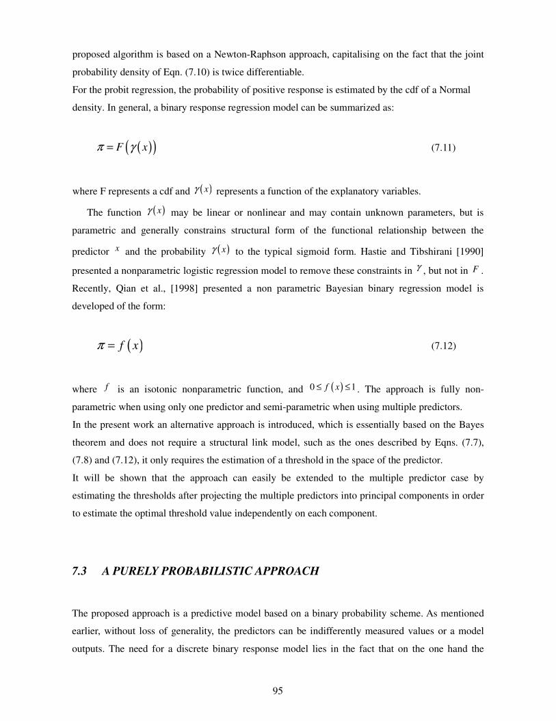
95
proposed algorithm is based on a Newton-Raphson approach, capitalising on the fact that the joint
probability density of Eqn. (7.10) is twice differentiable.
For the probit regression, the probability of positive response is estimated by the cdf of a Normal
density. In general, a binary response regression model can be summarized as:
( )( )π γ= F x
(7.11)
where F represents a cdf and ( )γ x represents a function of the explanatory variables.
The function ( )γ x may be linear or nonlinear and may contain unknown parameters, but is
parametric and generally constrains structural form of the functional relationship between the
predictor x and the probability ( )γ x to the typical sigmoid form. Hastie and Tibshirani [1990]
presented a nonparametric logistic regression model to remove these constraints in γ , but not in F .
Recently, Qian et al., [1998] presented a non parametric Bayesian binary regression model is
developed of the form:
( )π = f x
(7.12)
where f is an isotonic nonparametric function, and ( )0 1≤ ≤f x . The approach is fully non-
parametric when using only one predictor and semi-parametric when using multiple predictors.
In the present work an alternative approach is introduced, which is essentially based on the Bayes
theorem and does not require a structural link model, such as the ones described by Eqns. (7.7),
(7.8) and (7.12), it only requires the estimation of a threshold in the space of the predictor.
It will be shown that the approach can easily be extended to the multiple predictor case by
estimating the thresholds after projecting the multiple predictors into principal components in order
to estimate the optimal threshold value independently on each component.
7.3 A PURELY PROBABILISTIC APPROACH
The proposed approach is a predictive model based on a binary probability scheme. As mentioned
earlier, without loss of generality, the predictors can be indifferently measured values or a model
outputs. The need for a discrete binary response model lies in the fact that on the one hand the
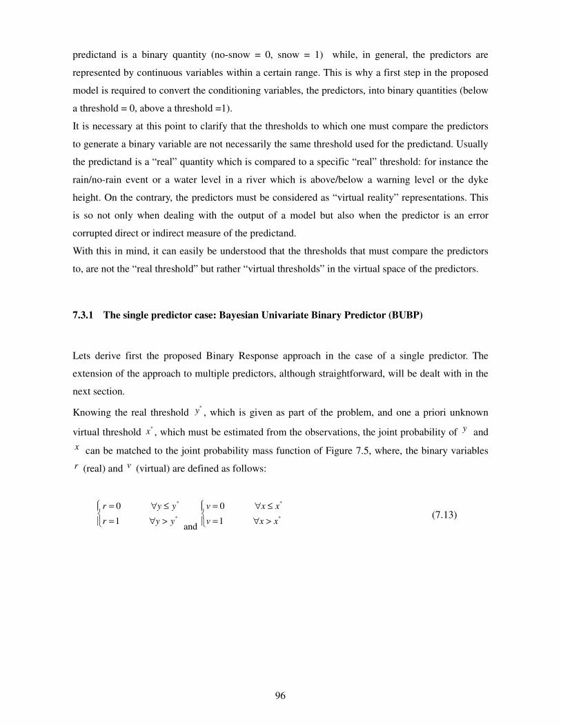
96
predictand is a binary quantity (no-snow = 0, snow = 1) while, in general, the predictors are
represented by continuous variables within a certain range. This is why a first step in the proposed
model is required to convert the conditioning variables, the predictors, into binary quantities (below
a threshold = 0, above a threshold =1).
It is necessary at this point to clarify that the thresholds to which one must compare the predictors
to generate a binary variable are not necessarily the same threshold used for the predictand. Usually
the predictand is a “real” quantity which is compared to a specific “real” threshold: for instance the
rain/no-rain event or a water level in a river which is above/below a warning level or the dyke
height. On the contrary, the predictors must be considered as “virtual reality” representations. This
is so not only when dealing with the output of a model but also when the predictor is an error
corrupted direct or indirect measure of the predictand.
With this in mind, it can easily be understood that the thresholds that must compare the predictors
to, are not the “real threshold” but rather “virtual thresholds” in the virtual space of the predictors.
7.3.1 The single predictor case: Bayesian Univariate Binary Predictor (BUBP)
Lets derive first the proposed Binary Response approach in the case of a single predictor. The
extension of the approach to multiple predictors, although straightforward, will be dealt with in the
next section.
Knowing the real threshold *y , which is given as part of the problem, and one a priori unknown
virtual threshold *x , which must be estimated from the observations, the joint probability of y and
x can be matched to the joint probability mass function of Figure 7.5, where, the binary variables
r (real) and v (virtual) are defined as follows:
*
*
0
1
= ∀ ≤
= ∀ >
r y y
r y y and
*
*
0
1
= ∀ ≤
= ∀ >
v x x
v x x
(7.13)
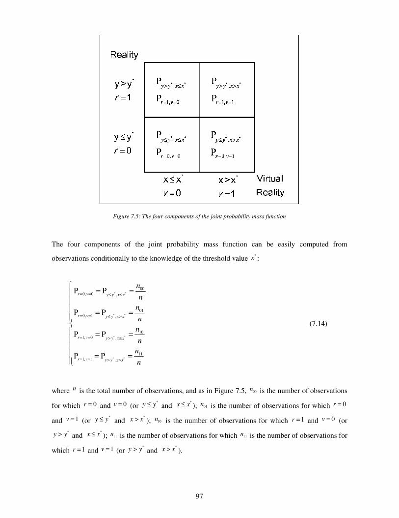
97
Figure 7.5: The four components of the joint probability mass function
The four components of the joint probability mass function can be easily computed from
observations conditionally to the knowledge of the threshold value *
x :
* *
* *
* *
* *
00
0, 0 ,
01
0, 1 ,
10
1, 0 ,
11
1, 1 ,
P P
P P
P P
P P
= = ≤ ≤
= = ≤ >
= = > ≤
= = > >
= =
= = = = = =
r v y y x x
r v y y x x
r v y y x x
r v y y x x
n
n
n
n
n
n
n
n
(7.14)
where n is the total number of observations, and as in Figure 7.5, 00n is the number of observations
for which 0=r and 0=v (or *≤y y and
*≤x x ); 01n is the number of observations for which 0=r
and 1=v (or *≤y y and
*>x x ); 10n is the number of observations for which 1=r and 0=v (or
*>y y and *≤x x ); 11n is the number of observations for which 11n is the number of observations for
which 1=r and 1=v (or *>y y and
*>x x ).
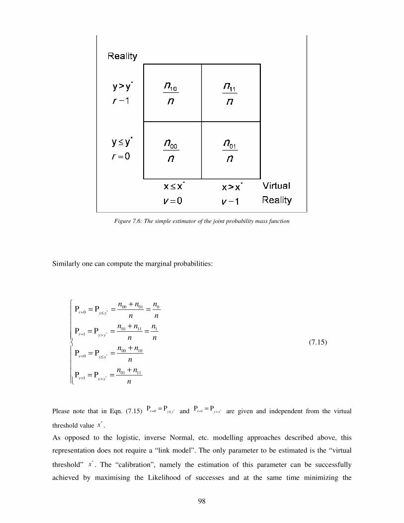
98
Figure 7.6: The simple estimator of the joint probability mass function
Similarly one can compute the marginal probabilities:
*
*
*
*
00 01 0
0
10 11 1
1
00 10
0
01 11
1
P P
P P
P P
P P
r y y
r y y
v x x
v x x
n n n
n n
n n n
n n
n n
n
n n
n
= ≤
= >
= ≤
= >
+= = =
+ = = =
+ = =
+ = =
(7.15)
Please note that in Eqn. (7.15) *0P P
r y y= ≤= and *1
P Pr y y= >
= are given and independent from the virtual
threshold value *x .
As opposed to the logistic, inverse Normal, etc. modelling approaches described above, this
representation does not require a “link model”. The only parameter to be estimated is the “virtual
threshold” *
x . The “calibration”, namely the estimation of this parameter can be successfully
achieved by maximising the Likelihood of successes and at the same time minimizing the
99
Likelihood of failures.
These Likelihoods can be easily defined on the basis of the probabilities of the predictor conditional
upon the observations, that can be derived by means of the Bayes theorem:
* *
* *
* * * *
* *
* *
* * * *
* *
* *
* * * *
00
, 00
0 000 10 00 10, ,
01
, 01
1 001 11 01 11, ,
1
,
0 1
, ,
PP P
P P
PP P
P P
PP P
P P
≤ ≤
= = ≤ ≤
≤ ≤ > ≤
≤ >
= = > ≤
≤ > > >
> ≤
= = ≤ >
≤ ≤ > ≤
= = = =+ +
+
= = = =+ +
+
= = =+
y y x x
v r x x y y
y y x x y y x x
y y x x
v r x x y y
y y x x y y x x
y y x x
v r x x y y
y y x x y y x x
n
nnn n n n
n n
n
nnn n n n
n n
n
* *
* *
* * * *
0
10
00 10 00 10
11
, 11
1 101 11 01 11, ,
PP P
P P
> >
= = > >
≤ > > >
= ++
= = = =+ + +
y y x x
v r x x y y
y y x x y y x x
nnn n n n
n n
n
nnn n n n
n n
(7.16)
When dealing with only one predictor the problem is easily solved by searching, in only one
dimension, the optimal threshold value which maximises the following Likelihood function, which
expresses the probability of successes given the threshold and the observations:
( )
( ) ( )
* * * *
* * * *
* *
*
0 0 1 1
, , * *
00 11
P P P P
P P
P P
s v r v r x x y y x x y y
y y x x y y x x
y y y y
L x
n x n x
= = = = ≤ ≤ > >
≤ ≤ > >
≤ >
= =
= ∝ (7.17)
while, at the same time, minimises the Likelihood function which expresses the probability of
failures given the threshold and the observations:
( )
( ) ( )
* * * *
* * * *
* *
*
1 0 0 1
, , * *
01 10
P P P P
P P
P P
f v r v r x x y y x x y y
y y x x y y x x
y y y y
L x
n x n x
= = = = > ≤ ≤ >
≤ > > ≤
≤ >
= =
= ∝ (7.18)
this can be formulated as follows:
100
( ) ( ){ } ( ) ( ) ( ) ( )*
* * * * * *
00 11 01 10L L− = −
s fxMax x x n x n x n x n x
(7.19)
The search of the threshold value can be in the positive direction if there is a positive correlation
between reality and virtual reality, namely when both predictand and predictor generally grow or
decrease at the same time, or it can be in the negative direction if the correlation is negative. A
simple solution to this problem is to compute the two thresholds in the opposed directions and then
select the one that produces the largest value of the objective function.
Once the threshold value *x is found, it is now easy to perform a prediction. The predictive scheme
is now:
* * *
*
* * *
* * *
*
* * *
P
PP
P
PP
≤ ≤ ∀ ≤
≤
≤ > ∀ >
> ≤ ∀ ≤
>
> > ∀ >
=
=
y y x x x x
y y x
y y x x x x
y y x x x x
y y x
y y x x x x
(7.20)
In this case, as opposed to what was done to “calibrate” the threshold (and generally what is also
done to validate the model in terms of POD or FAR) the conditionality is no more on the
observations, which being in a in “predictive” mode, are now assumed to be unknown. The
conditional probabilities to be used are then the probabilities of the real event conditional upon the
occurrence of the virtual one.
The probabilities appearing in Eqns. (7.19) can now be derived using the Bayes theorem as
follows:
101
* *
* *
* * * *
* *
* *
* * * *
* *
* *
* * * *
00
, 00
0 000 01 00 01, ,
01
, 01
0 100 01 00 01, ,
1
,
1 0
, ,
PP P
P P
PP P
P P
PP P
P P
≤ ≤
= = ≤ ≤
≤ ≤ ≤ >
≤ >
= = ≤ >
≤ ≤ ≤ >
> ≤
= = > ≤
> ≤ > >
= = = =+ +
+
= = = =+ +
+
= = =+
y y x x
r v y y x x
y y x x y y x x
y y x x
r v y y x x
y y x x y y x x
y y x x
r v y y x x
y y x x y y x x
n
nnn n n n
n n
n
nnn n n n
n n
n
* *
* *
* * * *
0
10
10 11 10 11
11
, 11
1 110 11 10 11, ,
PP P
P P
> >
= = > >
> ≤ > >
= ++
= = = =+ + +
y y x x
r v y y x x
y y x x y y x x
nnn n n n
n n
n
nnn n n n
n n
(7.21)
Using the predictive probability *P>y y x (only one of the two is needed since * *P 1 P
≤ >= −
y y x y y x ) one can
decide whether *>i
y y or *≤i
y y according to:
*
*
*
*
1P
2
1P
2
>
>
> ∀ >
≤ ∀ ≤
i i
i i
i y y x
i y y x
y y
y y
(7.22)
7.3.2 The multi-predictor case: Bayesian Multivariate Binary Predictor (BMBP)
When multiple predictors are used, the problem can still be easily solved after transforming the
ensemble of predictors into Empirical Orthogonal Functions also known as principal components,
by means of an ortho-normal transformation [Stephenson, 2000; Press et al., 1992].
Given a set of n observations of the predictand 1 2 � �n
y y yy and the simultaneous set of n
observations of m predictors
11 12 1
21 22 2
1 2
�
��� � � �
�
m
m
n n nm
x x x
x x x
x x x
X
(7.23)

102
the first step is the standardization of the predictors matrix and the computation of the predictors
correlation matrix.
This requires the estimation of:
1 2
1 2
µ µ µ
σ σ σ
� �
� �
m
m
µ
σ
(7.24)
where µj and σ
j are respectively the estimated mean and the estimated standard deviation for the
thj predictor, as well as of the correlation matrix:
12 1
21 2
1 2
1
1
1
1
ρ ρ
ρ ρ
ρ ρ
�
��� � �
�
m
m
m m
Σ
(7.25)
Once the correlation matrix is known, it is possible to decompose it into the eigenvalues matrix
1
2
0 0
0 0
0 0
λ
λ
λ
�
��� � � �
�m
Λ
(7.26)
and the corresponding eigenvectors matrix
11 12 1
21 22 2
1 2
�
��� � � �
�
m
m
m m mm
p p p
p p p
p p p
P
(27)
using one of the available techniques, such as for instance the modified Jacobi method (Press et al.,
1992). In general, the eigenvalues and the corresponding eigenvectors are arranged in descending
order of importance, to give:
= TΣ P ΛP (7.28)
The eigenvector matrix represents a rotation of coordinates in the predictors space in order to obtain
set of new predictors which are independent one from another.
Therefore the following new independent predictors are computed:
103
11 1 12 2 1
1 2
11 12 1
21 1 22 2 2
21 22 2
1 2
1 2
1 1 2 2
1 2
µ µ µ
σ σ σ
µ µ µ
σ σ σ
µ µ µ
σ σ σ
− − − − − − = − − −
�
�
� ��
� � � �� � � �
�
�
m m
m
m
m m
m
m
m m mm
n n nm m
m
x x x
p p px x x
p p p
p p px x x
X
(7.29)
Owing to this ortho-normal transformation one reaches two objectives. The first one is that all the
predictors are independent from one another, which allows to derive the relevant thresholds for each
component independently from the others using the single component technique. The second
objective is to possibly reduce the number of “effective” predictors when the original ones are
highly correlated among them. This can be done by looking at the sorted eigenvalues and retaining
only the dominant components (the columns of XXXX � corresponding to the highest values of their
relevant eigenvalues λ ).
Because all the components are independent, as mentioned earlier, the thresholds can now be
derived following the procedure described in the previous section.
Once all the thresholds have been derived, one must compute the overall conditional probabilities.
The interesting thing is that, because the predictors are independent, the conditional probability of
the 2m
possible 0 1− states of the m components can be obtained as follows as the product of the
individual conditional probabilities:
* *
* *
1
1
P P
P P
≤ ≤=
> >=
=
=
∏
∏
� �
� �
j
j
m
y y x y yj
m
y y x y yj
x
x
(7.30)
where:
* * *
*
* * *
* * *
*
* * *
P
PP
P
PP
≤ ≤ ∀ ≤
≤
> ≤ ∀ >
≤ > ∀ ≤
>
> > ∀ >
=
=
� � � �
�
� � � �
� � � �
�
� � � �
j j
j
j j
j j
j
j j
x x y y x x
x y y
x x y y x x
x x y y x x
x y y
x x y y x x
(7.31)
For example, in the case of three predictors, the following expression holds:
( ) ( ) ( ) ( ) ( ) ( ) ( ) ( ) ( ) ( ) ( ) ( )1 * 1 2 * 2 3 * 3 1 * 1 2 * 2 3 * 3* * * *, ,P P P P
≤ > > ≤ ≤ ≤ > ≤ > ≤=
x x x x x x y y x x y y x x y y x x y y (7.32)
104
Once the overall conditional probabilities have been obtained, using the Bayes theorem one can
estimate the required probabilities of a real event conditional upon the state of all predictors,
namely:
**
*
* ** *
**
*
* ** *
P PP
P P P P
P PP
P P P P
≤≤
≤
≤ >≤ >
>>
>
≤ >≤ >
=
+
=+
�
�
� �
�
�
� �
y yy y
y y
y y y yy y y y
y yy y
y y
y y y yy y y y
x
x
x x
x
x
x x
(7.33)
Finally, using the obtained predictive probability *P> �y y x (only one of the two is needed since
* *P 1 P≤ >
= −� �y y y yx x ) one can decide whether *>
iy y or *≤
iy y according to:
*
*
*
*
1P
2
1P
2
>
>
> ∀ >
≤ ∀ ≤
�
�
i i
i ii
i y y
i y y
y y
y y
x
x
(7.34)
7.4 EXAMPLES OF APPLICATION
The BMBP and a method based on the Logistic regression (LOG) were applied on the 7 datasets
presented in Paragraph 7.1 ( the sub case SSO has too few data to be processed, as already
explained in Paragraph 7.1.4), using half of the data for calibration while the other half was
reserved for validation.
Every AMSU-B FOV processed has been classified as snowing (r=1) or not-snowing (r=0)
considering the presence or not of precipitation without discriminating between cloudy and clear
condition.
For each subset the two models proposed and the SSA are compared evaluating the POD and the
FAR indexes, previously described in Chapter 5, defined as:
105
00
00 01
11
inf
10 11
10
10 00
01
01 11
nonsnowing
snow
nonsnowing
snowing
nPOD
n n
nPOD
n n
nFAR
n n
nFAR
n n
= +
=+
= + = +
(7.35)
where:
PODnonsnowing: is the probability of correct detection of non snowing cases
PODsnowing: is the probability of correct detection of snowing cases
FARnonsnowing: is the percentage of incorrect non snowing cases
FARsnowing: is the percentage of incorrect snowing cases
The SSA, evaluated on the same datasets used to validate the BMBP and the LOG models, was used
as a snowing/no snowing model in order to estimate as snowing the FOVS showing an estimated
rain-rate higher than zero.
Two figures are presented for each of the data sub-set. The first one, composed by four quadrants,
shows the BMBP calibration (upper left quadrant) and validation (upper right quadrant) results, and
LOG calibration (lower left quadrant) and validation (lower right quadrant) results.
The second figure shows the SSA results.
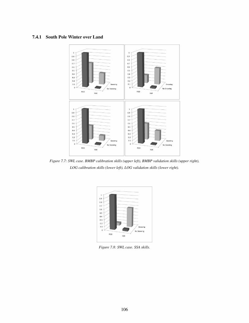
106
7.4.1 South Pole Winter over Land
Figure 7.7: SWL case. BMBP calibration skills (upper left), BMBP validation skills (upper right),
LOG calibration skills (lower left), LOG validation skills (lower right).
Figure 7.8: SWL case. SSA skills.
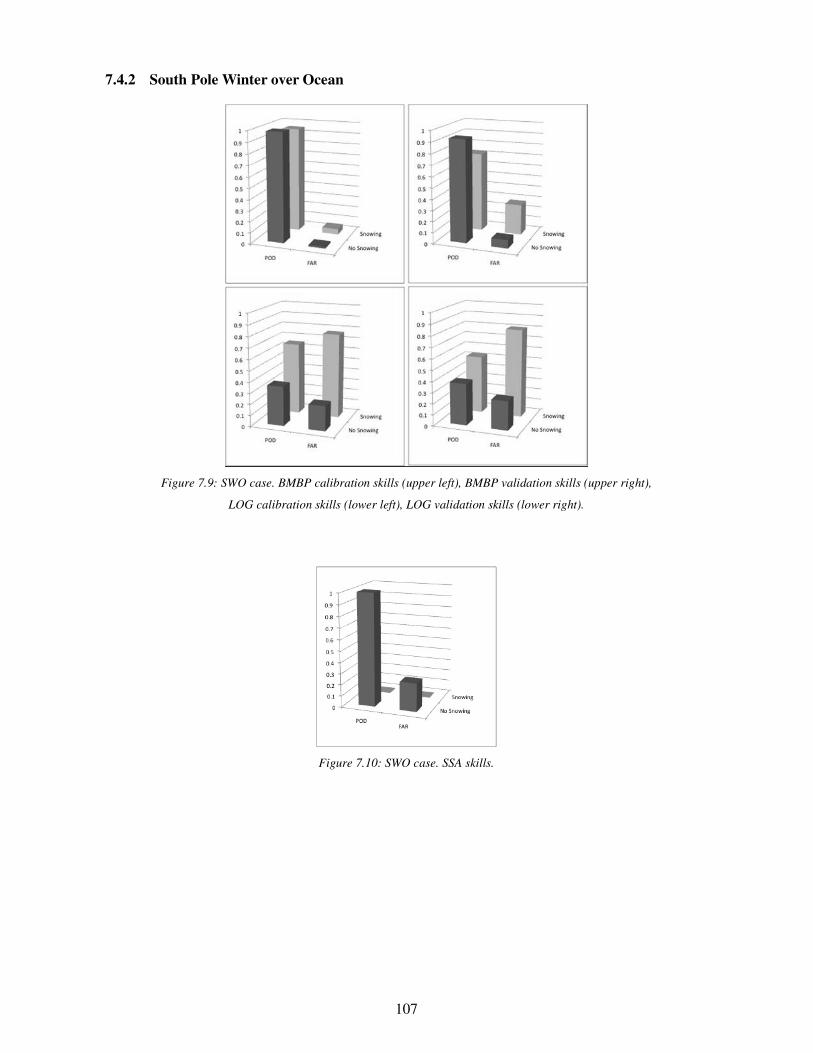
107
7.4.2 South Pole Winter over Ocean
Figure 7.9: SWO case. BMBP calibration skills (upper left), BMBP validation skills (upper right),
LOG calibration skills (lower left), LOG validation skills (lower right).
Figure 7.10: SWO case. SSA skills.
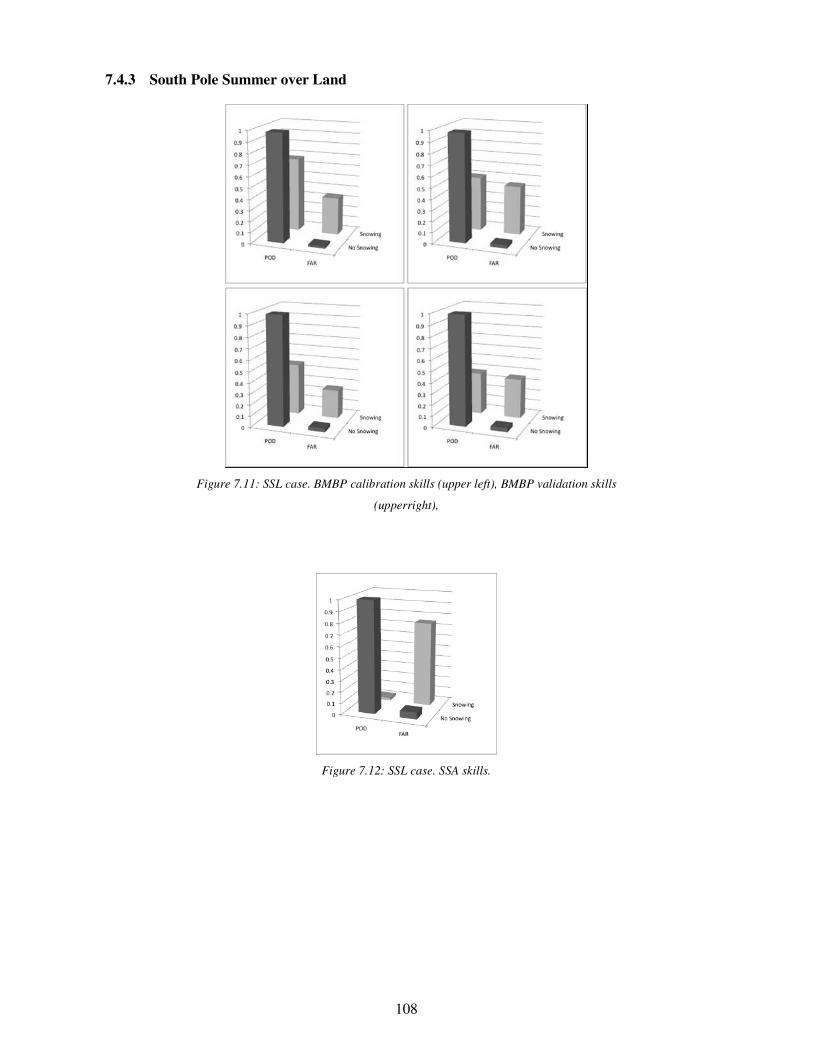
108
7.4.3 South Pole Summer over Land
Figure 7.12: SSL case. SSA skills.
Figure 7.11: SSL case. BMBP calibration skills (upper left), BMBP validation skills
(upperright),
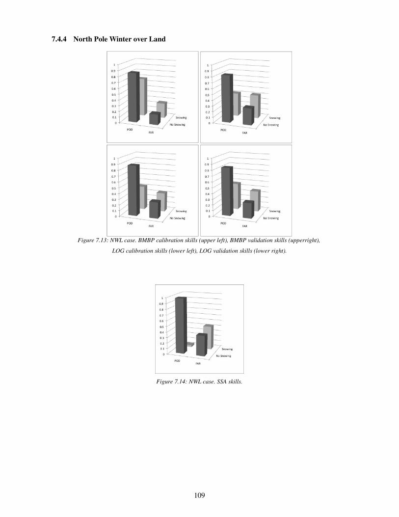
109
7.4.4 North Pole Winter over Land
Figure 7.14: NWL case. SSA skills.
Figure 7.13: NWL case. BMBP calibration skills (upper left), BMBP validation skills (upperright),
LOG calibration skills (lower left), LOG validation skills (lower right).
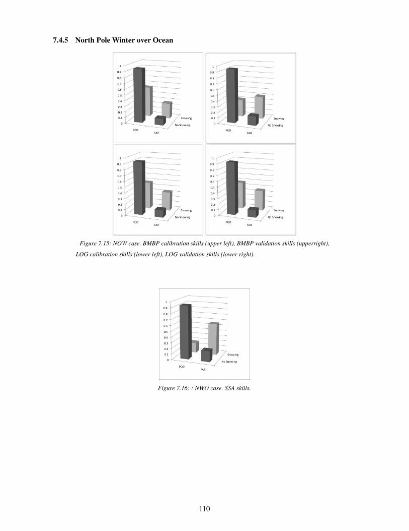
110
7.4.5 North Pole Winter over Ocean
Figure 7.16: : NWO case. SSA skills.
Figure 7.15: NOW case. BMBP calibration skills (upper left), BMBP validation skills (upperright),
LOG calibration skills (lower left), LOG validation skills (lower right).

111
7.4.6 North Pole Summer over Land
Figure 7.17: NSL case. BMBP calibration skills (upper left), BMBP validation skills (upperright),
LOG calibration skills (lower left), LOG validation skills (lower right).
Figure 7.18: NSL case. SSA skills.
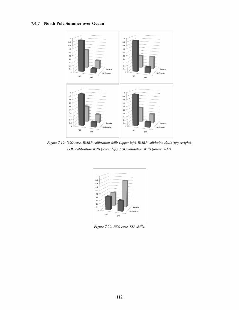
112
7.4.7 North Pole Summer over Ocean
Figure 7.19: NSO case. BMBP calibration skills (upper left), BMBP validation skills (upperright),
LOG calibration skills (lower left), LOG validation skills (lower right).
Figure 7.20: NSO case. SSA skills.
113
7.5 DISCUSSION
First of all it is important to compare the results obtained in calibrations with those obtained in
validation by BMBP and LOG to understand the robustness of the methods.
The method based on the Logistic regression shows a good agreement between calibrations and
validations in all the cases analyzed, giving always results coerent. The BMBP method, instead,
shows a good agreement between calibrations and validations only in five of the seven cases.
Nonetheless, even with a loss of performances, the verification results of the five cases outperform
those obtainable with the LOG approach. In addition the Logistic regression did not fully converge
in one of the cases (SWO).
In the BMBP validation for the SWL and the NWO cases (upper right quadrants of Figures. 7.7 and
7.15), the PODsnowing index is close to 0.3 and smaller than the FARsnowing index while in calibration
(upper left quadrant of Figures 7.7 and 7.15).the PODsnowing index results higher than 0.5 with a low
FARsnowing index.
These differences are probably due to the high sensitivity of the BMBP to the data selected. In fact
while the LOG method, filters the data though the assumption of a model (the logistic probability
distribution model, while the BMBP doesn’t.
One difficulty with the LOG method is that it may not reach convergence, as pointed out in the
SWO case (Figure 7.9). In fact the lower panels show results that are definitely not comparable with
the results obtained with the BMBP, which is due to the fact that the plotted results refer to the
highest iteration allowed.
Both models discriminate correctly more than 90% of the non snowing cases with a percentage of
wrong detection smaller than 10%. Only in the NWL and NSL cases, Figures 7.13 and 7.17, the
values of PODnonsnowing drop to 0.8 while the FAR nonsnowing index reach values close to 0.2.
The performances for the snowing cases, as expected, are not as good as those for the non snowing,
but almost in all the cases a probability of detection close to 0.5 is obtained by both models with a
percentage of wrong detections always below 50%. A paricular well predicted case is the SWO,
Figure 7.7, where BMBP is able to detect correctly 70% of the non snowing cases with a FARsnowing
index close to 0.2.
Figures 7.8, 7.10, 7.12, 7.14, 7.16, 7.18 and 7.10 show the performances of the SSA model in
detecting snowing and non snowing FOVs.
Except for the NSO case, Figure 7.20, where the PODnonsnowing drops below 0.5, in the remainng six
cases SSA is able to detect the non snowing events with a probability of detection comparable with
that showed for the two method proposed. The main differences appear when comparing the SSA
114
performance at detecting the snowing events. For the first 6 cases presented the values of the
PODsnowing index are close to 0.1 or lower with FARsnowing higher than 0.5.
The worst case examined is the NSO where the probability of correct detection is close to 0.4 but
the false alarm rate is 0.8.
The comparison allows to outline few points:
b) The BMBP and the LOG methods are able to discriminate with a relatively good
performance snowing and non snowing condition over the Polar regions.
c) The two proposed methods can be used as the basic pre-processing filter for improved
algorithms which aim at estimating the snow intensity, enhancing the percentage of
detections, and, more importantly, reducing the false alarm rate.
115
8 CONCLUSIONS
The work proposed in this thesis shows that a long way has still to be completed before an accurate
global operative precipitation estimation algorithm can become a candidate for an operational
status. The present work can only be considered as an important step forward, but in long walk.
As opposed to several existing approaches, the one proposed in this thesis outlines the importance
of treating the problem of rain rate estimations in two separate stages. First of all it is necessary to
estimate the probability of occurrence of precipitation and, conditional upon the fact that
precipitation will be non-null, it is then possible to estimate its intensity with appropriate
algorithms. The use of approaches where the same algorithm is used for both precipitating and non
precipitating clouds should be discouraged. As demonstrated in this research work, an accurate
snowing/non snowing preliminary analysis may consistently reduce the false alarm rate while
enhancing the probability of detection.
This thesis also highlights the importance of a multispectral approach. The implemented algorithms,
namely the Logistic Regression approach as well as the Bayesian Multivariate Binary Response,
allow to combine measurements from different types of sensors and models, thus increasing the
ability in discriminating the physical information. Moreover they extract the essential features of
the signals through an Empirical Orthogonal Function (Principal Components) approach, and can
therefore be applied to a wide variety of sensors thus avoiding the need for specific frequencies for
their application.
Another issue of the uttermost importance stemming from the thesis work is the need of
experimental data to be used as ground truths. The use of meteorological re-analyses should be
discouraged, since these inevitably produce biased and inefficient algorithms when used in
forecasting mode.
The availability of a new generation of satellites with Lidar and CloudRadar on-board represents an
essential tool for calibrating precipitating cloud detection algorithms. The future launch of ESA’s
EarthCARE, a single platform with a payload of two active sounders (lidar and radar) and two
complementary passive instruments (multi-spectral imager and a broadband radiometer), will
represents an important step forward also for the family of problems presented in this thesis.
Finally one must acknowledge that the methods presented in this thesis have been applied to the
challenging problem of detecting snowfall over snow and ice surface with encouraging results. The
application of the proposed techniques to more detailed case studies at mid-latitude is expected to
improve the rain-rate estimation and consequently to give an important contribution for improving
of the validation of NWP forecast and allowing the generation of a more robust precipitation

116
database for climate use.
117
References
Anderson G. P., S. A. Clough, F. X. Kneizys, J. H. Chetwood, and E. P. Shettle, AFGL atmospheric
constituent profiles (0–120 km), AFGL Tech. Rep., AFGL-TR-0110, 48 pp., Air Force Geophys.
Lab., Bedford, Mass., 1986.
Bauer A., M. Godon, J. Carlier, Q. Ma, andR .H. Tipping, Absorption by H20 and H20-N2 mixtures
at 153 GHz, J.Quant. SpectroscR. adiat. Transfer,50, 463-475, 1993.
Bauer A., M. Godon, J. Carlier, and Q. Ma., Water vapor absorption in the atmospheric window at
239 GHz, J. Quant.S pectroscR. adiat. Transfer,53, 411-423, 1995
Bauer A., M. Godon, J. Carlier, and R.R. Gamache, Absorption of a H20-CO2 mixture in the
atmospheric window at 239 GHz; H20-CO2 linewidths and continuum, J. Mol. Spectrosc. 176, 45-
57, 1996.
Becker G.E. , and Autler S.H., Water Vapor Absorption of Electromagnetic Radiation in the
Centimeter Wavelength Range, Phys. Rev. , Vol. 70, 300-307, 1946.
Bennartz, R., and G. W. Petty, The sensitivity of microwave remote sensing observations of
precipitation to ice particle size distributions, J. Appl. Meteorol., 40, 345–364, 2001.
Bohren C.F., and Huffman D.R., Absorption and Scattering of Light by Small Particles. Wiley and
Sons, 1983.
Boukabara S. A. , S. A. Clough, J.-L. Moncet, A. F. Krupnov,M. Tretyakov, and V. V. Parshin,
Uncertainties in the temperature dependence of the line coupling parameters of the microwave
Oxygen band: Impact study, IEEE Trans. Geosci. Remote Sens., vol. 43, no. 5, pp. 1109–1114, May
2005.
Chen F.W. , A.M. Leckman, and D.H. Staelin, Passive Microwave Signatures of Arctic Snowstorms
Observed from Satellites, IEEE International Geoscience and Remote Sensing Symposium,
Toulouse, France, 21-25 July 2003
Cimini D., Ed R. Westwater, Albin J. Gasiewski, Marian Klein, Vladimir Ye. Leuski, and Sally G.
Dowlatshahi, The Ground-Based Scanning Radiometer: A Powerful Tool for Study of the Arctic
Atmosphere, IEEE Transactions On Geoscience And Remote Sensing, Vol. 45, No. 9, September
2007.
Choudhury B. J. , T. J. Schmugge, A. Chang, and R. W. Newton, Effect of surface roughness on the
microwave emission from soils, J. Geophys. Res., vol. 84, no. C9, pp. 5699–5706, 1979
Clough S.A., F.X. Kneizys, R. Davies, R. Gamache and R. Tipping, Theoretical line shape for H2O
vapour; Application to the continuum. Atmospheric water vapour, A. Deepak, T.D. Wilkerson and
L.H. Ruhnke, eds. (Academic, New York,), pp. 25-46, 1980.
Clough S.A., F.X. Kneizys and R.W. Davis: Line shape and the water vapour continuum,
Atmospheric research 23, 229-241, 1989.
118
Draper, D., Assessment and Propagation of Model Uncertainty, Journal of the Royal Statistical
Society. Series B (Methodological), 57(1):45-97, 1995.
Debye D., Polar Molecules, New York, Dover, 1929.
Deirmendjian D. , Electromagnetic Scattering on Spherical Polydispersions, New York, American
Elsevier Publishing Company, Inc., 1969.
Dudhia J. , D. Gill, K. Manning, W. Wang, and C. Bruyere, PSU/NCAR Mesoscale Modeling System
Tutorial Class Notes and Users’ Guide (MM5 Modeling System Version 3), Jan. 2005.
[Online]. Available:http://www.mmm.ucar.edu/mm5/documents/tutorial-v3-notes.html
Evans, K.F. and Stephens, G.L.: A new polarized atmospheric transfer model. J. Quant. Spectros.
Radiat. Transfer, 46, 412-423, 1991.
Evans, K. F., and G. L. Stephens, Microwave radiative transfer through clouds composed of
realistically shaped ice crystals: Part I. Single scattering properties, J. Atmos. Sci., 52, 2041–
2057,1995.
Ferraro, R. R., F. Weng, N. C. Grody, and L. Zhao, Precipitation characteristics over land from
NOAA-15 AMSU Sensor, Geophys. Res. Lett., 27(17), 2669–2672, 2000.
Ferraro, R. R., and N. C. Grody (Contributing authors), Scientific Assessment of High-Frequency
Radiometer Channels on the GPM Core Satellite for Warm and Light Rain plus Snow
Measurements, GPM Report, NASA/Goddard Space Flight Center, MD, 2001.
Frenkel L., and D. Woods, The microwave absorption by H20 vapor and its mixtures with other
gases between 100 and 300 Gc/s, Proc. IEEE, 54(4), 498-505, 1966
Frisch S., Shupe M., Djalova I., Feingold G. and Pellot M., The retrieval of stratus cloud droplet
effective radius with cloud radars, Journal of Atmosp. and Ocean Technology. 19, 2002.
Fu Q., K.N. Liou, Parameterization of the radiative properties of cirrus clouds, Journal of
Atmosph. Sciences, 50, 13, 1993.
Fu Q., An accurate parameterization of the solar radiative properties of cirrus clouds for climate
models, Journal of Climate, 9, 2058 2082, 1996.
Fu Q., K. N. Liou, M. C. Cribb, T. P. Charlock, and A. Grossman, Multiple scattering
parameterization in thermal infrared radiative transfer, Journal of atmospheric Sciences., 54,
2799-2812, 1997.
Fu Q., Yang Ping, and W. B. Sun, An accurate parameterization of the infrared radiative properties
of cirrus clouds for climate models, Journal of Climate, 11, 2223 2237, 1998.
Fu Q. et al.: Modelling of scattering and absorption by non spherical cirrus ice particles at thermal
infrared wavelengths, Journal of Atmosph. Sciences, 56, 2937 2947, 1999.
Gasiewski A. J., Microwave Radiative Transfer in Hydrometeors, in Michael A. Janssen (ed.),
Atmospheric Remote Sensing by Microwave Radiometry, New York, J. Wiley & Sons, Inc., , pp.
91-144, 1993.
119
Godon M., J. Carlief, and A. Bauer, Laboratory studies of water vapor absorptionin the
atmospheric window at 213 GHz, J. Quant. Spectrosc. Radiat. Transfer, 47, 275-285,1992.
Goody, R.M., and Yung Y.L., Atomspheric Radiation. Theoretical Basis. Oxford University Press,
1989.
Hänel G., Advanced Geophysics, 19, 73, 1976.
Hänel G and Lehmann M.: Beitr. Physics Atmos., 54, 57, 1981.
Hansen, J.E.: Multiple scattering of polarized light in planetary atmosphere. Part I: The doubling
method. J. Atmos. Sci., 28, 120-125, 1971.
Hastie, T.J. and Tibshirani R.J., Generalized Additive Models, Chapman and Hall, London, 1990.
Heymsfield A.J.: Properties of Tropical and Mid Latitude ice cloud particles ensembles. Part I:
Median mass diameters and terminal velocities, Journal of Atmosph. Sciences, 2573-2591, 60,
2003a.
Heymsfield A.J.: Properties of Tropical and Mid Latitude ice cloud particles ensembles. Part II:
Application for mesoscale and climate model,. Journal of Atmosph. Sciences, 2592-2611, 60,
2003b.
Heymsfield A.J., Matrosov S. and Baum B: Ice Water Path-Optical depth relationships for cirrus
and deep startiform ice cloud layer,. Journal of Applied Meteorology, 1369-1390, 42, 2003.
Hewison T. J., S. J. English, Airborne Retrievals of Snow and Ice Surface Emissivity at Millimeter
Wavelengths,IEEE Transactions On Geoscience And Remote Sensing, Vol. 37, No. 4, July 1999.
Hewison T. J., Aircraft validation of clear air absorption models at millimeter wavelengths (89–183
GHz), J. Geophys. Res., vol. 111, no. D14, D14 303, 2006.
Hill R.J. , Water vapor-absorption line shape comparison using the 22-GHz line : The Van Vleck-
Weisskopf shape affirmed, Radio Science, Vol. 21, 447-451, May-June 1986.
Hong, G., Parameterization of scattering and absorption properties of nonspherical ice crystals at
microwave frequencies, J. Geophys. Res., 112, D11208, doi:10.1029/2006JD008364, 2007.
Katsumata, M., H. Uyeda, K. Iwanami, and G. Liu, The response of 36- and 89-GHz microwave
channels to convective snow clouds over ocean: Observations and modeling, J. Appl. Meteorol., 39,
2322–2335, 2000.
Kongoli, C., P. Pellegrino, R. R. Ferraro, C. Grody, and H. Meng, A new snowfall detection
algorithm over land using measurements from the Advanced Microwave Sounding Unit (AMSU),
Geophys. Res. Lett.,30(14), 1756, doi:10.1029/2003GL017177, 2003.
Kurucz, R. L. , 1997, The solar irradiance by computation, available from:
http://kurucz.harvard.edu/sun/IRRADIANCE/, 1997.
120
Liebe H.J., The atmospheric water vapor continuum below 300 GHz, lnt. J. Infrared Millimeter
Waves, 5(2), 207-227, 1984.
Liebe H.J. and Layton D.H., Millimeter-wave properties of the atmosphere: Laboratory studies and
propagation modeling, Nat. Telecom. and Inform.Admin., Boulder, CO, NIT Rep. 87-24, 1987
Liebe H.J., G.A. Hufford and T. Manabe, A model for the complex permittivity of water at
frequencies below 1 THz, Internat. J. Infrared and mm Waves, Vol. 12, pp. 659-675, 1991.
Liebe H.J., G.A. Hufford, and M.G. Cotton, Propagation modeling of moist air and suspended
water/ice particles at frequencies below 1000 GHz, AGARD Conf. Proc. 542, 3.1-3.10, 1993.
Liljegren, J. C., Improved retrievals of temperature and water vapor using a twelve channel
microwave radiometer. In Proceedings of the Thirteenth Atmospheric Radiation Measurement
(ARM) Science Team Meeting, ARM-CONF-2003. U.S. Department of Energy, Washington, D.C,
2003.
Liljegren J. C. , S. A. Boukabara, K. Cady-Pereiria, and S. A. Clough, The effect of the half-width of
the 22-GHz water vapor line on retrievals of temperature and water vapor profiles with a 12
channel microwave radiometer, IEEE Trans. Geosci. Remote Sens., vol. 43, no. 5, pp. 1102–1108,
May 2005.
Lindley, D. V., The choice of variables in multiple regression (with discussion), J. R. Statist. Soc. B,
30:31-67,1968..
Liou, K. N.: Radiation and Cloud Processes in the Atmosphere. Oxford University press, 1992.
Liu, G., and J. A. Curry, Precipitation characteristics in the GIN Seas determined using satellite
microwave data, J. Geophys. Res., 102(13), 987– 997, 1997.
Liu, G., and M. Katsumata, Studies on snowfall retrieval from satellite high frequency microwave
observations, Preprints, 6th Symposium on Integrated Observing Systems, Am. Meteorol. Soc.,
Orlando, FL, 2002.
Liu, G. , Approximation of single scattering properties of ice and snow particles for high microwave
frequencies, J. Atmos. Sci., 61, 2441– 2456,2004.
Loffredo G.: Processi di diffusione in atmosfera: confronto con dati sperimentali. Thesis work,
ADGB, Phys. Dept., University of Bologna, 2000.
Marshall J.S. and W. Palmer, The distribution of rain drops with size, J. Meteorology, 5,165-166,
1948.
Masuda K., Takashima T and Takayama Y.: Emissivity of pure and sea waters for the model sea
surface in the infrared window regions,. Remote Sensing of Environment, 24, 313-329, 1988.
McCullagh, P. and Nelder J.A., 1989. Generalized Linear Models (second edition). Chapman and
Hall, London.
121
Mugnai, A., S. Di Michele, E.A. Smith, F. Baordo, P. Bauer, B. Bizzarri , P. Joe, C. Kidd,
F.S.Marzano, A. Tassa, J. Testud, and G.J. Tripoli, Snowfall measurements by the proposed
European GPM mission. Measuring Precipitation from Space: EURAINSAT and the Future.
(V. Levizzani, P. Bauer, and F.J. Turk, Eds.),655-674, Springer 2007.
Mattioli V. , E. R. Westwater, S. I. Gutman, and V. R. Morris, Forward Model Studies of Water
Vapor using Scanning Microwave Radiometers, Global Positioning System, and Radiosondes
during the Cloudiness Inter-Comparison Experiment, IEEE Transactions on Geoscience and
Remote Sensing,. 43(5), pp. 1012-1021, 2005.
Mattioli V. , E. R. Westwater, D. Cimini, J. C. Liljegren, B. M. Lesht, S. I. Gutman, and F- J-
Schmidlin, Analysis of Radiosonde and Ground-Based Remotely Sensed PWV Data from the 2004
North Slope of Alaska Arctic Winter Radiometric Experiment, Journal of atmospheric and oceanic
technology, vol.24, pp 415-431, 2007.
Mätzler C., IET Electrmagnetic Wave Series 52,Thermal Microwave Radiation: Applications for
Remote sensing,Chapter 2, 255-99. 2006.
Menoux V., R. Le Doucen, C. Boulet, A. Roblin and A.M. Bouchardy, Collision induced absorption
in the fundamental Band of N2. Applied Optics 32. 263-268, 1993.
Miller, A. J., Algorithm AS 274, Least squares routines to supplement those of Gentleman. Appl.
Statist., 41, 458–478, 1992.
Miskolczi F., R. Rizzi, R. Guzzi e M.M. Bonzagni: A New High Resolution Atmospheric Transmittance
Code and its Application in the Field of Remote Sensing. Atti del IRS 88: Current Problems in
Atmospheric Radiation, Lille 18-24, 388-391, 1988a.
Miskolczi F., R. Guzzi ed R.Rizzi, A New High Resolution Atmospheric Transmittance Code and its
Application for the Calculation of the Weighting Functions under Tropical Conditions. Atti dello
International Satellite Land-Surface Climatology Project (ISLSCP), Niamey, Niger 25-29, 1988b.
Miskolczi F., M. Bonzagni, R. Guzzi, High Resolution Atmospheric Radiance-Transmittance Code
(HARTCODE). Meteorology and Environmental Sciences, World Scientific Pub. Co. 1990, pp.
743-790, 1990.
Miskolczi F. and Rizzi R., CO2 Q-Band Line Mixing in HARTCODE. Technical note DFUB 97-14,
October, 1997.
Mitchell D.L., Effective diameter in radiation transfer: general definition, applications and
limitations. Journal of the Atmosph. Sciences, 59, 2330-2346, 2002.
Nelder, J.A. and Wedderburn RW.M., 1972, Generalized linear models, Journal of the Royal Statistical
Society, A, 135:370-384.
Paukkunen, A., V. Antikainen, and H. Jauhiainen, Accuracy and performance of the new Vaisala
RS90 radiosonde in operational use. Preprints, 11th Symp. on Meteorological Observations and
Instrumentation, Albuquerque, NM, Amer. Meteor. Soc., CD-ROM, 4.5, 2001.
Payne V. H. , J. S. Delamere, K. E. Cady - Pereira, R. R. Gamache, J - L. Moncet, E. Mlawer, S. A.
Clough, Air - broadened half - widths of the 22 GHz and183 GHz water vapor lines, submitted to
122
IEEE Transactions in Geoscience and Remote Sensing, 2007.
Press, W.H., Teukolsky, S.A., Vetterling, W.T. and Flannery, B.P., Numerical Recipes in Fortran.
The Art of Scientific Computing (Second Edition). Cambridge University Press. Cambridge, UK
1992.
Pulliainen J. , K. Tigerstedt, W. Huining, M. Hallikainen, C. Mätzler, A. Wiesmann, and C.
Wegmüller, Retrieval of geophysical parameters with integrated modeling of land surfaces and
atmosphere (models/ inversion algorithms), European Space Agency, Final Report of the
ESTEC contract No. 11706/95/NL/NB(SC), Oct 1998.
Qian S.S., M. Lavine and C.A. Stow, Bayesian nonparametric binary response regression models
with application in environmental management, manuscript submitted.
http://citeseer.ist.psu.edu/qian98bayesian.html, 1998.
Racette, P. E., and Coauthors, Measurement of low amounts of precipitable water vapor using
ground-based millimeterwave radiometry. J. Atmos. Oceanic Technol., 22, 317– 337, 2005.
Raftery, A. E., Bayesian model selection in structural equation models. In K. A. Bollen and J. S.
Long (Eds.), Testing Structural Equation Models, pp. 163-180. Newbury Park, Calif. Sage, 1993..
Raftery, A. E., F. Balabdaoui, T. Gneiting, and M. Polakowski. Using Bayesian model averaging to
calibrate forecast ensembles, Tech. Rep. 440, Dep. of Stat., Univ. of Wash., Seattle, 2003.
Ray P.S, Appl. Opt., 11, 1836, 1972.
Rinsland C.P., J.S. Zander, J.S Namkung, C.B. Farmer and R.H. Norton: Stratospheric infrared
continuum absorption observed by the ATMOS instrument., J. Geophys. Res. 94, 16303-16322, 1989.
Rosenkranz P.W., Water vapor microwave continuum absorption: A comparison of measurements and
models, Radio ScienceV, olume 33, Number 4, Pages9 19-928, July-August,1998
Rosenkranz P. W., “Correction to ‘Water vapor microwave continuum absorption: A comparison of
measurements and models’,” Radio Sci., vol. 34, no. 4, p. 1025, 1999.
Rosenkranz P.W., Radiative Transfer Solution Using Initial Values in a Scattering and Absorbing
Atmosphere with Surface Reflection, IEEE Transactions On Geoscience And Remote Sensing, Vol.
40, NO. 8, AUGUST 2002
Rosenkranz P. W., personal communication, 2007.
Segelstein D., The complex refractive index of water. M.S. Thesis. University of Missouri, Kansas City.
1981.
Sekhon, R. S., and R. C. Srivastava, Snow size spectra and radar reflectivity, J. Atmos. Sci., 27, 299–
307, 1970.
Sihvola A. H. , Self-consistency aspects of dielectric mixing theories, IEEE Trans. Geosci. Remote
Sens., vol. 27, no. 4, pp. 403-415, Jul. 1989.
Skofronick-Jackson, G.M., J.A. Weinman, and D. Chang, Observation of Snowfall over Land by
Microwave Radiometry from Space, Proc. 2002 IEEE Int'l Geosci. Remote Sensing Symp., Toronto,
123
Canada, Vol. 3,1866-1868, June 2002.
Staelin,D.H., andF.W. Chen, Precipitation observations near 54and 183GHz using NOAA-15
Satellite, IEEE Trans., Geosci. Rem. Sens., 38(5), 2322– 2332, 2000.
Staelin D. H. and C. Surussavadee, Precipitation retrieval accuracies for geomicrowave
sounders, IEEE Transactions On Geoscience And Remote Sensing, VOL. 45, NO. 10, OCTOBER
2007
Stephenson, D. (2000), http://www.uib.no/people/ngbnk/kurs/notes/node87.html
Surussavadee C. and D. H. Staelin, Comparison of AMSU millimeter-wave satellite observations,
MM5/TBSCAT predicted radiances, and electromagnetic models for hydrometeors, IEEE Trans.
Geosci. Remote Sens., vol. 44, no. 10, pp. 2667-2678, Oct. 2006.
Surussavadee C.and David H. Staelin, Millimeter-Wave Precipitation Retrievals and Observed-versus-
Simulated Radiance Distributions: Sensitivity to Assumptions. Journal of the Atmospheric Sciences.
Vol. 64, Iss. 11, pp. 3808–3826, 2007.
Surussavadee C.; Staelin, David H.; Chadarong, Virat; McLaughlin, Dennis; Entekhabi, Dara,
Comparison of NOWRAD, AMSU, AMSR-E, TMI, and SSM/I surface precipitation rate Retrievals over
the united states great plains, Geoscience and Remote Sensing Symposium, 2007. IGARSS 2007.
IEEE International , vol., no., pp.3923-3926, 23-28 July 2007
Surussavadee, C.; Staelin, D.H., Global Millimeter-Wave Precipitation Retrievals Trained With a
Cloud-Resolving Numerical Weather Prediction Model, Part I: Retrieval Design, Geoscience and
Remote Sensing, IEEE Transactions on , vol.46, no.1, pp.99-108, Jan. 2008
Timofeyev Y.M. and M.V. Tonkov: Effect of the induced Oxygen absorption band on the
transformation of radiation in the 6th region of the Earth's atmosphere. Izvestiya, Atmospheric and
Ocean Physics 14, 437-441, 1978.
Van de Hulst H. C. , Light Scattering by Small Particles, New York, Dover Publications Inc.,1981.
Vrugt, J. A., and B. A. Robinson, Treatment of uncertainty using ensemble methods: Comparison of
sequential data assimilation and Bayesian model averaging, Water Resour. Res., 43, W01411,
doi:10.1029/2005WR004838, 2007.
Wang J. R. and B. J. Choudhury, Remote sensing of soil moisture content over bare field at 1.4 GHz
frequency, J. Geophys. Res., vol. 86, pp. 5277–5282, 1981.
Wang, J. R., P. E. Racette, and M. E. Triesky, Retrieval of precipitable water vapor by the
Millimeter-wave Imaging Radiometer in the Arctic region during FIRE-ACE, IEEE Trans., Geosci.
Rem. Sens., 39(3), 595– 605, 2001.
Warren S. G, Optical constants of ice from the ultraviolet to microwave, Applied Optics,Vol.23, N.8,
1984.
Weismann A., Mätzler C., Microwave emission model of layered snowpacks, Remote Sens.
Environ.,70, 307-16, 1999.
Wieliczka D. M., Weng S. and Querry M.R.: Wedge shaped cell for highly absorbent liquids:
124
infrared optical constants of water, Applied Optics, 28, 9, 1989.
Wiscombe W.J., JQSRT,16,637,1976.
Yang, P and K. N. Liou, Geometric optics integral equation method for light scattering
by nonspherical ice crystals. Applied Optics, 35, 33, 6568 6584, 1996.
Yang, P., and K. N. Liou, Single scattering properties of complex ice crystals in terrestrial
atmosphere. Contr. Atmos. Phys.., 71, 223 248.
Yang, P., H. Wei, H. L. Huang, B. A. Baum, Y. X. Hu, G. W. Kattawar, M. I. Mishchenko, and Q.
Fu, Scattering and absorption property database for nonspherical ice particles in the near
through far infrared database. Appl. Opt., 44, 26, 2005, 1998.
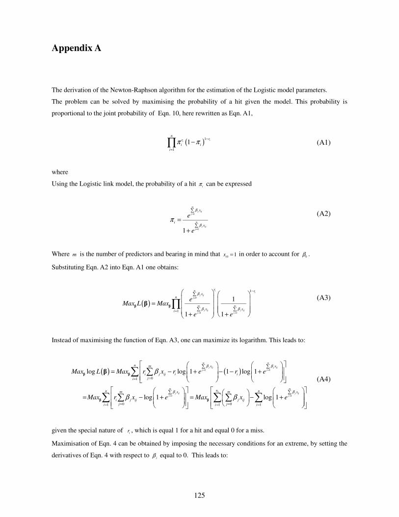
125
Appendix A
The derivation of the Newton-Raphson algorithm for the estimation of the Logistic model parameters.
The problem can be solved by maximising the probability of a hit given the model. This probability is
proportional to the joint probability of Eqn. 10, here rewritten as Eqn. A1,
( )1
1
1π π−
=
−∏ ii
nrr
i i
i
(A1)
where
Using the Logistic link model, the probability of a hit πi can be expressed
0
01
β
βπ
=
=
∑
∑=
+
m
j ijj
m
j ijj
x
ix
e
e
(A2)
Where m is the number of predictors and bearing in mind that 0
1=i
x in order to account for 0
β .
Substituting Eqn. A2 into Eqn. A1 one obtains:
( )0
0 0
1
1
1
1 1
β
β β
=
= =
−
=
∑
∑ ∑
= + +
∏
m ii
j ijj
m m
j ij j ijj j
r rx
n
x xi
eMax L Max
e e
β ββ
(A3)
Instead of maximising the function of Eqn. A3, one can maximize its logarithm. This leads to:
( ) ( )0 0
1
0 0
01
0 01 1
log log 1 1 log 1
log 1 log 1
β β
β β
β
β β
= =
= =
==
= == =
∑ ∑
∑ ∑
= − + − − +
= − + = − +
∑
∑ ∑
∑
∑ ∑
m m
j ij j ijj j
m m
j ij j ijj j
n m x x
i j ij i iji
nn m mx x
i j ij j ijj ji i
Max L Max r x r e r e
Max r x e Max x e
β β
β β
β
1=
∑
n
i
(A4)
given the special nature of i
r , which is equal 1 for a hit and equal 0 for a miss.
Maximisation of Eqn. 4 can be obtained by imposing the necessary conditions for an extreme, by setting the
derivatives of Eqn. 4 with respect to βj equal to 0. This leads to:
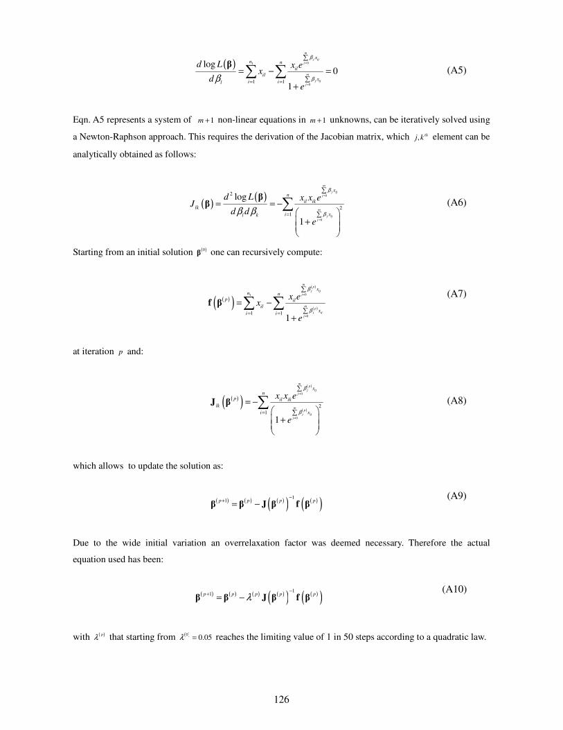
126
( ) 01
01 1
log0
1
β
ββ
=
== =
∑
∑= − =
+
∑ ∑
m
j ijj
m
j ijj
xn n
il
ilx
i il
d L x ex
de
β (A5)
Eqn. A5 represents a system of 1+m non-linear equations in 1+m unknowns, can be iteratively solved using
a Newton-Raphson approach. This requires the derivation of the Jacobian matrix, which , thj k element can be
analytically obtained as follows:
( )( ) 0
0
2
2
1
log
1
β
ββ β
=
=
=
∑
∑
= = −
+
∑
m
j ijj
m
j ijj
xn
il ik
lk
xil k
d L x x eJ
d de
ββ (A6)
Starting from an initial solution ( )0β one can recursively compute:
( )( )( )
( )
01
01 1
1
β
β
=
== =
∑
∑= −
+
∑ ∑
mp
j ijj
mp
j ijj
xn n
p il
ilx
i i
x ex
e
f β (A7)
at iteration p and:
( )( )( )
( )
0
0
2
1
1
β
β
=
=
=
∑
∑
= −
+
∑
mp
j ijj
mp
j ijj
xn
p il ik
lk
xi
x x e
e
J β (A8)
which allows to update the solution as:
( ) ( ) ( )( ) ( )( )1
1−
+= −
p p p pβ β J β f β
(A9)
Due to the wide initial variation an overrelaxation factor was deemed necessary. Therefore the actual
equation used has been:
( ) ( ) ( ) ( )( ) ( )( )1
1 λ−
+= −
p p p p pβ β J β f β
(A10)
with ( )λ p that starting from ( )00.05λ = reaches the limiting value of 1 in 50 steps according to a quadratic law.
127
AKNOWLEDGEMENTS
This work has been supported by a grant from IMAA, Istituto di Metodologie per l’Analisi
Ambientale.
First of all, I am very grateful to my research supervisor, Professor Rolando Rizzi, for his guidance,
support and patience.
I would like to thank Doctor Vincenzo Levizzani for his help and suggestions, Dr. Filomena
Romano and Dr. Domenico Cimini.
I would like to thank all the Atmospheric Dynamic Group colleagues of Bologna: Doctor Alessio
Bozzo, Doctor Tiziano Maestri, Doctor Valerio Lucarini and Doctor Ennio Tosi for their helps and
suggestions.
I would like to thank Professor Staelin and Doctor Phil Rosenkranz for giving me the opportunity to
work as a visiting student in the Remote Sensing and Estimation Group at the M.I.T., and for their
guidance.
I also would like to thank Professor Stalein and Dr Chinnawat “POP” Surussavadee for giving me
the opportunity to work with their rain-rate algorithm.
I would like to thank my family for its support and in particular my father that helped me more than
I thought.
I would like to thank Giorgia and CASADUSE for their support and their unbelievable patience.