Applied Mathematical Modelling 34 (2010) 294–300

Contents lists available at ScienceDirect

Applied Mathematical Modelling

journal homepage: www.elsevier .com/locate /apm

A note on single-machine scheduling with decreasing time-dependentjob processing times

Ji-Bo WangOperations Research and Cybernetics Institute, School of Science, Shenyang Institute of Aeronautical Engineering, Shenyang 110136, China

a r t i c l e i n f o

Article history:Received 27 November 2007Received in revised form 13 April 2009Accepted 29 April 2009Available online 9 May 2009

Keywords:SchedulingSingle-machineTime-dependent processing timesResource allocation

0307-904X/$ - see front matter � 2009 Elsevier Incdoi:10.1016/j.apm.2009.04.018

E-mail address: wangjibo75@yahoo.com.cn

a b s t r a c t

In this note we consider some single-machine scheduling problems with decreasing time-dependent job processing times. Decreasing time-dependent job processing times meansthat its processing time is a non-increasing function of its execution start time. We presentpolynomial solutions for the sum of squared completion times minimization problem, andthe sum of earliness penalties minimization problem subject to no tardy jobs, respectively.We also study two resource constrained scheduling problems under the same decreasingtime-dependent job processing times model and present algorithms to find their optimalsolutions.

� 2009 Elsevier Inc. All rights reserved.

1. Introduction

Machine scheduling problems with start time dependent processing times have received increasing attention in recentyears. Researchers have formulated this phenomenon into different models and solved different versions of the problemfor various criteria. Extensive surveys of different scheduling models and problems involving start time dependent process-ing times can be found in Alidaee and Womer [1], and Cheng et al. [2]. More recently, Wang and Xia [3] considered varioussingle-machine and flow-shop scheduling problems with decreasing linear deterioration of job processing times. Wang andXia [4,5] considered flow-shop problems involving job deterioration and dominating machines. Gawiejnowicz et al. [6] con-sidered two single-machine bicriterion scheduling problems with time-dependent job processing times. Wang et al. [7] con-sidered two-machine flow-shop scheduling with simple linear job deterioration. Janiak and Kovalyov [8] considered theproblem of scheduling n jobs executed by a human in a contaminated area. Wang [9] considered the general, no-wait andno-idle flow-shop scheduling problems with deteriorating jobs. These studies assumed that the processing time of a jobis a decreasing function of its starting time. Gawiejnowicz [10] considered two single-machine makespan minimizationscheduling problems with proportionally deteriorating jobs. In the first problem, the machine is not continuously availablefor processing but the number of non-availability periods, and the start time and the end time of each period are known inadvance. In the second problem, the machine is available all the time but for each job a ready time and a deadline are de-fined. He showed that both problems are NP-hard. Wang et al. [11] considered single-machine scheduling with deterioratingjobs in which the jobs are constrained by a series-parallel graph constraint. They proved that the problem can be solved inpolynomial time. Leung et al. [12] considered the scheduling problem on parallel and identical machines where the jobs areprocessed in batches and the processing time of each job is a step function of its waiting time. They showed that the problemis NP-hard in the strong sense. Lee and Wu [13] considered multi-machine scheduling with deteriorating jobs and scheduled

. All rights reserved.

J.-B. Wang / Applied Mathematical Modelling 34 (2010) 294–300 295

maintenance. Tang and Liu [14] considered two-machine flowshop scheduling problems involving a batching machine withtransportation or deterioration consideration.

Generally, there are two types of models describing this kind of processes. The first type is devoted to the problems inwhich the job processing time is characterized by a non-decreasing function, and the second type concerns problems inwhich the job processing time is given by a non-increasing function. In this note we study the latter group of problems,i.e., single-machine scheduling problems with decreasing time-dependent job processing times. This model was proposedby Ho et al. [15]. The remaining part of this paper is organized as follows. In Section 2 we describe and formulate the prob-lem. In Sections 3 and 4 we consider the sum of squared completion times minimization problem and sum of earliness pen-alties minimization problem, respectively. In Section 5 we consider two resource constrained scheduling problems under thesame decreasing time-dependent job processing times model and present algorithms to solve them. The last section is theconclusion.

2. Model description

There are given a single machine and a set N ¼ fJ1; J2; . . . ; Jng of n independent and non-preemptive jobs, which are avail-able for processing at some time t0 P 0. Each job Jj has a normal processing time aj. Following Ho et al. [15] and Wang andXia [3], we assume that the actual processing time pj of job Jj is a non-increasing linear function of the job’s starting time, i.e.,

pj ¼ ajð1� ktÞ; ð1Þ

where aj P 0 and t P t0 is the job’s starting time. It is assumed that the decreasing rates satisfy the following condition:

k t0 þXn

j¼1

aj � amin

!< 1; ð2Þ

where amin ¼ mini¼1;2;...;nfaig. The condition ensures that all job processing times are positive in a feasible schedule (see also[15,3] for detailed explanations).

For a given schedule p ¼ ð½1�; ½2�; . . . ; ½n�Þ, Cj ¼ CjðpÞ represents the completion time of job Jj. In the remaining part of thepaper, all the problems considered will be denoted using the three-field notation scheme ajbjc introduced by Graham et al.[16].

3. Minimizing the sum of squared completion times

Townsend [17] considered a single machine scheduling problem with a quadratic cost function of completion times, i.e.,the sum of the quadratic job completion times. He showed that the problem 1jj

PC2

j can be solved optimally by the shortestprocessing time (SPT) rule. By using the job interchanging technique, we can show that the solution of Townsend’s still holdsfor the problem 1jpj ¼ ajð1� ktÞj

PC2

j .

Lemma 1. (Wang and Xia [3])For a given schedule p ¼ ð½1�; ½2�; . . . ; ½n�Þ with job processing times in the form of pj ¼ ajð1� ktÞ, ifjob J½1� starts at time 0 6 t0 <

1k �

Pnj¼1aj þ amin, then the makespan is equal to

Cmax ¼ t0 �1k

� �Yn

i¼1

ð1� ka½i�Þ þ1k; ð3Þ

if the makespan is C, then the starting time of the first job is

t0 ¼ C � 1k

� ��Yn

i¼1

ð1� ka½i�Þ þ1k:

Theorem 1. For the problem 1jpj ¼ ajð1� ktÞjP

C2j , an optimal schedule can be obtained by sequencing the jobs in non-decreas-

ing order of aj (i.e., the smallest normal processing time (SPT) rule).

Proof. Let p and p0 be two job schedules where the difference between p and p0 is a pair-wise interchange of two adjacentjobs Ji and Jj, i.e., p ¼ ðS1; Ji; Jj; S2Þ and p0 ¼ ðS1; Jj; Ji; S2Þ, where S1 and S2 are partial sequences, such that ai 6 aj. Let t denotethe completion time of the last job in S1. To show p dominates p0, it suffices to show that CjðpÞ 6 Ciðp0Þ andC2

i ðpÞ þ C2j ðpÞ 6 C2

j ðp0Þ þ C2i ðp0Þ. It is easy to derive the completion times of jobs Ji and Jj in p as

CiðpÞ ¼ t þ aið1� ktÞ ¼ t � 1k

� �ð1� kaiÞ þ

1k; ð4Þ

and

CjðpÞ ¼ t � 1k

� �ð1� kaiÞð1� kajÞ þ

1k: ð5Þ

296 J.-B. Wang / Applied Mathematical Modelling 34 (2010) 294–300

Similarly, the completion times of jobs Jj and Ji in p0 are

Cjðp0Þ ¼ t � 1k

� �ð1� kajÞ þ

1k; ð6Þ

and

Ciðp0Þ ¼ t � 1k

� �ð1� kajÞð1� kaiÞ þ

1k: ð7Þ

Based on Eqs. (5) and (7), we have CjðpÞ ¼ Ciðp0Þ. In addition, from (4) and (6), and ai 6 aj, we have CiðpÞ 6 Cjðp0Þ. HenceC2

i ðpÞ þ C2j ðpÞ 6 C2

j ðp0Þ þ C2i ðp0Þ; thus p dominates p0. This completes the proof. h

Corollary 1. For the problem 1jpj ¼ ajð1� ktÞjP

Chj , where h > 0; an optimal schedule can be obtained by sequencing the jobs in

non-decreasing order of aj (i.e., the SPT rule).

4. Minimizing the sum of earliness penalties

In this section we consider the problem of minimization of the sum of earliness penalties subject to no tardy jobs underthe assumption that the actual processing times of the jobs follow the model given in (1). For the classical problem, there aresome results in Chang and Schneeberger [18], and Qi and Tu [19]. We assume that all the jobs have a common due date d andthe release time is 0. Let Ej ¼ d� Cj be the earliness of job Jj. The objective is to minimize

PgðEjÞ, where gðxÞ is a strictly

increasing function. The problem is denoted as 1jpj ¼ ajð1� ktÞjP

gðEjÞ. A schedule is feasible if and only if there is no tardyjob in the schedule. For any optimal schedule, it is obvious that (i) the completion time of the last job is d, and (ii) there is noidle time between the jobs, and idle time can only exist before the first job, i.e., the t0 is a decision variable.

Theorem 2. For the problem 1jpj ¼ ajð1� ktÞjP

gðEjÞ, an optimal schedule can be obtained by sequencing the jobs in non-increasing order of aj (i.e., the largest normal processing time (LPT) rule), where the starting time of the first job ist0 ¼ d� 1

k

� ��Qni¼1ð1� kaiÞ þ 1

k :

Proof. Consider an optimal schedule p. Suppose there are two adjacent jobs Ji and Jj in p with job Ji being followed by job Jj

and ai < aj. Let the completion time of job Jj be Cj. Performing an adjacent pair-wise interchange of jobs Ji and Jj to get a newschedule p0, we have,

Ci ¼ Cj �1k

� ��ð1� kajÞ þ

1k; Ej ¼ d� Cj; Ei ¼ d� Cj �

1k

� ��ð1� kajÞ �

1k;

C 0i ¼ Cj;C0j ¼ Cj �

1k

� ��ð1� kaiÞ þ

1k; E0i ¼ d� Cj; E

0j ¼ d� Cj �

1k

� ��ð1� kaiÞ �

1k:

From (2) and ai < aj, we have Cj � 1k < 0, E0j < Ei; and E0i ¼ Ej: Hence gðE0iÞ þ gðE0jÞ < gðEjÞ þ gðEiÞ.

The completion times of the jobs processed after jobs Ji and Jj are not affected by the interchange, and the completiontimes of the jobs processed before jobs Ji and Jj are also not affected by the interchange either (from Lemma 1). Hence thevalue of the objective function under p0 is strictly less than that under p. This contradicts the optimality of p and proves thetheorem. h

When gðxÞ ¼ x, and the objective function isP

wjEj, we have the following result:

Corollary 2. For the problem 1jpj ¼ ajð1� ktÞjP

wjEj, an optimal schedule can be obtained by sequencing the jobs in non-increasing order of aj=½wjð1� kajÞ�, where the starting time of the first job is t0 ¼ ðd� 1

k�Qn

i¼1ð1� kaiÞ þ 1k.

Remark: When gðxÞ ¼ x,Pn

j¼1wjgðEjÞ ¼ dPn

j¼1wj �Pn

j¼1wjCj. Since dPn

j¼1wj is a constant, the weighted sum of completiontimes maximization problem can be solved by sequencing the jobs in non-increasing order of aj=½wjð1� kajÞ�, while theweighted sum of completion times minimization problem can be solved by sequencing the jobs in non-decreasing orderof aj=½wjð1� kajÞ� (Bachman et al. [20]).

5. Resource constrained problems

Bachman and Janiak [21] first considered single-machine scheduling with job processing times dependent on the startingmoments of job execution and on the amounts of resource allocation to the jobs. They proved that the makespan minimi-zation problem is NP-hard. They also gave some properties of the optimal resource allocation. Zhao et al. [22] consideredsingle-machine scheduling with deteriorating jobs where the release times of the jobs depend on the amounts of resourceallocation. For two resource constrained scheduling problems, they gave optimal algorithms to find the optimal resourceallocations. In this section we consider the following model:

J.-B. Wang / Applied Mathematical Modelling 34 (2010) 294–300 297

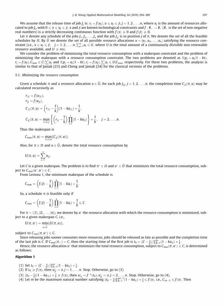
We assume that the release time of job Jj is: rj ¼ f ðujÞ;a 6 uj 6 b, j ¼ 1;2; . . . ;n, where uj is the amount of resources allo-cated to job Jj, with 0 6 a 6 uj 6 b; a and b are known technological constraints and f : Rþ ! Rþ (Rþ is the set of non-negativereal numbers) is a strictly decreasing continuous function with f ðaÞP 0 and f ðbÞP 0.

Let p denote any schedule of the jobs J1; J2; . . . ; Jn and the job J½j� is in position j of p. We denote the set of all the feasibleschedules by P. By eU we denote the set of all possible resource allocations u ¼ ½u1;u2; . . . ;un� satisfying the resource con-straint (i.e., a 6 uj 6 b; j ¼ 1;2; . . . ;n;

Pnj¼1uj 6 U; where U is the total amount of a continuously divisible non-renewable

resource available, and U P naÞ.We consider the problem of minimizing the total resource consumption with a makespan constraint and the problem of

minimizing the makespan with a resource consumption constraint. The two problems are denoted as 1jpj ¼ ajð1� ktÞ;rj ¼ f ðujÞ;Cmax 6 Cj

Puj and 1jpj ¼ ajð1� ktÞ; rj ¼ f ðujÞ;

Puj 6 UjCmax, respectively. For these two problems, the analysis is

similar to that of Janiak [23] and Cheng and Janiak [24] for the classical versions of the problems.

5.1. Minimizing the resource consumption

Given a schedule p and a resource allocation u 2 eU , for each job J½j�, j ¼ 1;2; . . . ;n, the completion time C½j�ðp;uÞ may becalculated recursively as

r½1� ¼ f ðu½1�Þ;r½j� ¼ f ðu½j�Þ;

C ½1�ðp;uÞ ¼ r½1� �1k

� �ð1� ka½1�Þ þ

1k;

C ½j�ðp;uÞ ¼max16i6j

r½i� �1k

� �Yj

l¼i

ð1� ka½l�Þ( )

þ 1k; j ¼ 2; . . . ;n:

Thus the makespan is

Cmaxðp;uÞ ¼max16i6nfC ½j�ðp;uÞg:

Also, for p 2 P and u 2 eU , denote the total resource consumption by

Uðp;uÞ ¼Xn

j¼1

u½j�:

Let C is a given makespan. The problem is to find p� 2 P and u� 2 eU that minimizes the total resource consumption, sub-ject to Cmaxðu�;u�Þ 6 C.

From Lemma 1, the minimum makespan of the schedule is

Cmax ¼ f ðbÞ � 1k

� �Yn

i¼1

ð1� kaiÞ þ1k:

So, a schedule p is feasible only if

Cmax ¼ f ðbÞ � 1k

� �Yn

i¼1

ð1� kaiÞ þ1k6 C:

For p ¼ ð½1�; ½2�; . . . ; ½n�Þ, we denote by u� the resource allocation with which the resource consumption is minimized, sub-ject to a given makespan C, i.e.,

Uðp;u�Þ ¼minu2eU fUðp; uÞg;

subject to Cmaxðp;u�Þ 6 C.Since releasing jobs sooner consumes more resources, jobs should be released as late as possible and the completion time

of the last job is C. If Cmaxðp; �Þ ¼ C, then the starting time of the first job is t0 ¼ C � 1k

� ��Qni¼1ð1� ka½i�Þ þ 1

k :

Hence, the resource allocation u� that minimizes the total resource consumption, subject to Cmaxðp;u�Þ 6 C, is determinedas follows:

Algorithm 1

(1) Set t0 ¼ C � 1k

� ��Qni¼1ð1� ka½i�Þ þ 1

k :

(2) If t0 P f ðaÞ, then u�½j� ¼ a; j ¼ 1; . . . ;n: Stop. Otherwise, go to (3).

(3) t0 � 1k

� �ð1� ka½1�Þ þ 1

k P f ðaÞ, then u�½1� ¼ f�1ðt0Þ;u�½j� ¼ a; j ¼ 2; . . . ;n: Stop. Otherwise, go to (4).(4) Let m be the maximum natural number satisfying t0 � 1

k

� �Qm�1i¼1 ð1� ka½i�Þ þ 1

k 6 f ðaÞ; i.e., C½m�1� 6 f ðaÞ: Then

298 J.-B. Wang / Applied Mathematical Modelling 34 (2010) 294–300

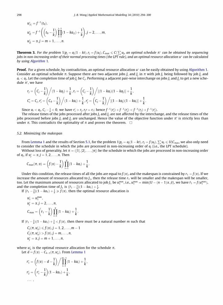
u�½1� ¼ f�1ðt0Þ;

u�½j� ¼ f�1 t0 �1k

� �Yj�1

i¼1

ð1� ka½i�Þ þ1k

!; j ¼ 2; . . . ;m;

u�½j� ¼ a; j ¼ mþ 1; . . . ;n:

Theorem 3. For the problem 1jpj ¼ ajð1� ktÞ; rj ¼ f ðujÞ;Cmax 6 CjP

uj, an optimal schedule p� can be obtained by sequencingjobs in non-increasing order of their normal processing times (the LPT rule), and an optimal resource allocation u� can be calculatedby using Algorithm 1.

Proof. For a given schedule, by contradiction, an optimal resource allocation u� can be easily obtained by using Algorithm 1.Consider an optimal schedule p. Suppose there are two adjacent jobs Ji and Jj in p with job Ji being followed by job Jj andai < aj. Let the completion time of job Jj be Cj. Performing a adjacent pair-wise interchange on jobs Ji and Jj to get a new sche-dule p0, we have

rj ¼ Cj �1k

� ��ð1� kajÞ þ

1k; ri ¼ Cj �

1k

� ��½ð1� kaiÞð1� kajÞ� þ

1k;

C 0i ¼ Cj; r0i ¼ C0 �1k

� ��ð1� kaiÞ þ

1k; r0j ¼ Cj �

1k

� ��½ð1� kajÞð1� kaiÞ� þ

1k:

Since ai < aj, Cj � 1k < 0; we have r0i > rj; rj0 ¼ ri; hence f�1ðr0iÞ þ f�1ðr0jÞ < f�1ðrjÞ þ f�1ðr0iÞ.

The release times of the jobs processed after jobs Ji and Jj are not affected by the interchange, and the release times of thejobs processed before jobs Ji and Jj are unchanged. Hence the value of the objective function under p0 is strictly less thanunder p. This contradicts the optimality of p and proves the theorem. h

5.2. Minimizing the makespan

From Lemma 1 and the results of Section 5.1, for the problem 1jpj ¼ ajð1� ktÞ; rj ¼ f ðujÞ;P

uj 6 UjCmax, we also only needto consider the schedule in which the jobs are processed in non-increasing order of aj (i.e., the LPT schedule).

Without loss of generality, let p ¼ ð½1�; ½2�; . . . ; ½n�Þ be the schedule in which the jobs are processed in non-increasing orderof aj, if u�j ¼ a; j ¼ 1;2; . . . ;n. Then

Cmaxðp;aÞ ¼ f ðaÞ � 1k

� �Yn

i¼1

ð1� kaiÞ þ1k:

Under this condition, the release times of all the jobs are equal to f ðaÞ, and the makespan is constrained by r1 ¼ f ðaÞ. If weincrease the amount of resources allocated to J1, then the release time r1 will be smaller and the makespan will be smaller,too. Let the maximum amount of resources allocated to job J1 be umax

1 , i.e., umax1 ¼minfU � ðn� 1Þa; bg, we have �r1 ¼ f ðumax

1 Þ,and the completion time of J1 is �r1 � 1

k

� �ð1� ka1Þ þ 1

k.If �r1 � 1

k

� �ð1� ka1Þ þ 1

k P f ðaÞ; then the optimal resource allocation is

u�1 ¼ umax1 ;

u�j ¼ a; j ¼ 2; . . . ; n;

Cmax ¼ �r1 �1k

� �Yn

i¼1

ð1� kaiÞ þ1k:

If ð�r1 � 1kÞð1� ka1Þ þ 1

k < f ðaÞ; then there must be a natural number m such that

Cjðp;u�pÞ 6 f ðaÞ; j ¼ 1;2; . . . ;m� 1Cjðp;u�pÞ > f ðaÞ; j ¼ m; . . . ; n;

u�j ¼ a; j ¼ mþ 1; . . . ; n;

where u�p is the optimal resource allocation for the schedule p.Let d ¼ f ðaÞ � Ck�1ðp;u�pÞ. From Lemma 1

r�1 ¼ f ðaÞ � d� 1k

� ��Ym�1

i¼1

ð1� kaiÞ þ1k;

r�2 ¼ r�1 �1k

� �ð1� ka1Þ þ

1k;

. . . ;

J.-B. Wang / Applied Mathematical Modelling 34 (2010) 294–300 299

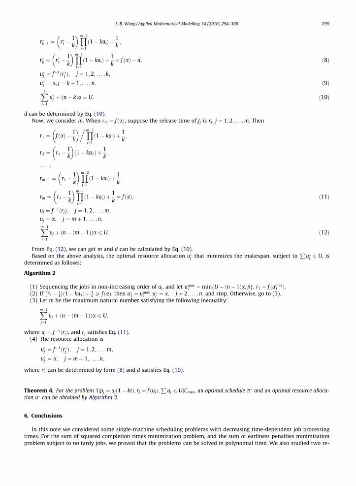
r�k�1 ¼ r�1 �1k

� �Ym�2

i¼1

ð1� kaiÞ þ1k;

r�k ¼ r�1 �1k

� �Ym�1

i¼1

ð1� kaiÞ þ1k¼ f ðaÞ � d; ð8Þ

u�j ¼ f�1ðr�j Þ; j ¼ 1;2; . . . ; k;

u�j ¼ a; j ¼ kþ 1; . . . ; n: ð9ÞXk

j¼1

u�j þ ðn� kÞa ¼ U: ð10Þ

d can be determined by Eq. (10).Now, we consider m. When rm ¼ f ðaÞ, suppose the release time of Jj is rj, j ¼ 1;2; . . . ;m. Then

r1 ¼ f ðaÞ � 1k

� ��Ym�1

i¼1

ð1� kaiÞ þ1k;

r2 ¼ r1 �1k

� �ð1� ka1Þ þ

1k;

. . . ;

rm�1 ¼ r1 �1k

� �Ym�2

i¼1

ð1� kaiÞ þ1k;

rm ¼ r1 �1k

� �Ym�1

i¼1

ð1� kaiÞ þ1k¼ f ðaÞ; ð11Þ

uj ¼ f�1ðrjÞ; j ¼ 1;2; . . . ;m;

uj ¼ a; j ¼ mþ 1; . . . ;n;Xm�1

j¼1

uj þ ðn� ðm� 1ÞÞa 6 U: ð12Þ

From Eq. (12), we can get m and d can be calculated by Eq. (10).Based on the above analysis, the optimal resource allocation u�j that minimizes the makespan, subject to

Pu�j 6 U, is

determined as follows:

Algorithm 2

(1) Sequencing the jobs in non-increasing order of aj, and let umax1 ¼minfU � ðn� 1Þa; bg; �r1 ¼ f ðumax

1 Þ:(2) If �r1 � 1

k

� �ð1� ka1Þ þ 1

k P f ðaÞ, then u�1 ¼ umax1 ;u�j ¼ a; j ¼ 2; . . . ;n; and stop. Otherwise, go to (3).

(3) Let m be the maximum natural number satisfying the following inequality:

Xm�1

j¼1

uj þ ðn� ðm� 1ÞÞa 6 U;

where uj ¼ f�1ðrjÞ, and rj satisfies Eq. (11).(4) The resource allocation is

u�j ¼ f�1ðr�j Þ; j ¼ 1;2; . . . ;m;

u�j ¼ a; j ¼ mþ 1; . . . ;n;

where r�j can be determined by form (8) and d satisfies Eq. (10).

Theorem 4. For the problem 1jpj ¼ ajð1� ktÞ; rj ¼ f ðujÞ;P

uj 6 UjCmax, an optimal schedule p� and an optimal resource alloca-tion u� can be obtained by Algorithm 2.

6. Conclusions

In this note we considered some single-machine scheduling problems with decreasing time-dependent job processingtimes. For the sum of squared completion times minimization problem, and the sum of earliness penalties minimizationproblem subject to no tardy jobs, we proved that the problems can be solved in polynomial time. We also studied two re-

300 J.-B. Wang / Applied Mathematical Modelling 34 (2010) 294–300

source constrained problems under the same job deterioration model. We presented an algorithm which can obtain the opti-mal schedule and the optimal resource allocation, respectively. Future research may consider more general time-dependentjob processing times types, or study the other objective functions.

Acknowledgement

We are grateful to the editor and an anonymous referee, whose constructive comments have led to a substantial improve-ment in the presentation of the paper. This research was supported by the Science Research Foundation of the EducationalDepartment of Liaoning Province, China, under grant number 20060662.

References

[1] B. Alidaee, N.K. Womer, Scheduling with time dependent processing times: review and extensions, J. Oper. Res. Soc. 50 (1999) 711–720.[2] T.C.E. Cheng, Q. Ding, B.M.T. Lin, A concise survey of scheduling with time-dependent processing times, Eur. J. Oper. Res. 152 (2004) 1–13.[3] J.-B. Wang, Z.-Q. Xia, Scheduling jobs under decreasing linear deterioration, Inform. Process. Lett. 94 (2005) 63–69.[4] J.-B. Wang, Z.-Q. Xia, Flow shop scheduling with deteriorating jobs under dominating machines, Omega 34 (2006) 327–336.[5] J.-B. Wang, Z.-Q. Xia, Flow shop scheduling problems with deteriorating jobs under dominating machines, J. Oper. Res. Soc. 57 (2006) d220–226.[6] S. Gawiejnowicz, W. Kurc, L. Pankowska, Pareto and scalar bicriterion optimization in scheduling deteriorating jobs, Comput. Oper. Res. 33 (2006) 746–

767.[7] J.-B. Wang, C.T. Ng, T.C.E. Cheng, L.L. Liu, Minimizing total completion time in a two-machine flow shop with deteriorating jobs, Appl. Math. Comput.

180 (2006) 185–193.[8] A. Janiak, M.Y. Kovalyov, Scheduling in a contaminated area: a model and polynomial algorithms, Eur. J. Oper. Res. 173 (2006) 125–132.[9] J.-B. Wang, Flow shop scheduling problems with decreasing linear deterioration under dominating machines, Comput. Oper. Res. 34 (2007) 2043–

2058.[10] S. Gawiejnowicz, Scheduling deteriorating jobs subject to job or machine availability constraints, Eur. J. Oper. Res. 180 (2007) 472–478.[11] J.-B. Wang, C.T. Ng, T.C.E. Cheng, Single-machine scheduling with deteriorating jobs under a series-parallel graph constraint, Comput. Oper. Res. 35

(2008) 2684–2693.[12] J.Y.T. Leung, C.T. Ng, T.C.E. Cheng, Minimizing sum of completion times for batch scheduling of jobs with deteriorating processing times, Eur. J. Oper.

Res. 187 (2008) 1090–1099.[13] W.-C. Lee, C.-C. Wu, Multi-machine scheduling with deteriorating jobs and scheduled maintenance, Appl. Math. Model. 32 (2008) 362–373.[14] L. Tang, P. Liu, Two-machine flowshop scheduling problems involving a batching machine with transportation or deterioration consideration, Appl.

Math. Model. 33 (2009) 1187–1199.[15] K.I.-J. Ho, J.Y.T. Leung, W.-D. Wei, Complexity of scheduling tasks with time-dependent execution times, Inform. Process. Lett. 48 (1993) 315–320.[16] R.L. Graham, E.L. Lawler, J.K. Lenstra, A.H.G. Rinnooy Kan, Optimization and approximation in deterministic sequencing and scheduling: a survey,

Annals Discrete Math. 5 (1979) 287–326.[17] W. Townsend, The single machine problem with quadratic penalty function of completion times: a branch-and-bound solution, Manage. Sci. 24 (1978)

530–534.[18] S. Chang, H. Schneeberger, Single machine scheduling to minimize weighted earliness subject to no tardy jobs, Eur. J. Oper. Res. 34 (1988) 221–230.[19] X. Qi, F.-S. Tu, Scheduling a single machine to minimize earliness penalties subject to the SLK due-date determination method, Eur. J. Oper. Res. 105

(1998) 502–508.[20] A. Bachman, T.C.E. Cheng, A. Janiak, C.T. Ng, Scheduling start time dependent jobs to minimize the total weighted completion time, J. Oper. Res. Soc. 53

(2002) 688–693.[21] A. Bachman, A. Janiak, Scheduling deteriorating jobs dependent on resources for the makespan minimization, in: Operations Research Proceedings

2000: Selected Papers of the Symposium on Operations Research (OR 2000), Dresden, September 2000, pp. 29–34.[22] C.-L. Zhao, H.-Y. Tang, Single machine scheduling problems with deteriorating jobs, Appl. Math. Comput. 161 (2005) 865–874.[23] A. Janiak, Time-optimal control in a single machine problem with resource constraints, Automatica 22 (1986) 745–747.[24] T.C.E. Cheng, A. Janiak, Resource optimal control in some single machine scheduling problem, IEEE Trans. Automat. Control 39 (1994) 1243–1246.