Journal of Econometrics 4 (1976) 295-300. 0 North-Holland Publishing Company

A NOTE ON THE BAYESIAN ESTIMATION OF SOLOW’S DISTRIBUTED LAG MODEL

Robert S. GUTHRIE

University of New Mexico, Albuquerque, N.M. 87131, U.S.A.

Received July 1974, revised version received October 1975

This note develops the Bayesian estimation of the parameters of Solow’s distributed lag model with implicit autocorrelation of disturbances in its autoregressive form. The estimation tech- nique extends Chetty’s method for independent disturbances. The results of some Monte Carlo experiments are given comparing point estimates from the posterior distributions with the maximum likelihood estimates. The characteristics of the Bayesian and maximum likelihood estimates are very similar.

1. Introduction

Chetty (1971) has presented a useful application of Bayesian analysis to estimate the parameters of the Pascal distributed lag model developed by Solow (1960). The moving average form of the model is

where L is the lag operator and this is equivalent to the autoregressive form

(1 -AL)lY, = cr(1 -A)rXr+Vt, (2)

where u, = (1 -;lL)‘ul. If the disturbances in the moving average form, u, are assumed to be independently distributed then the disturbances in the auto- regressive form, V, must be correlated. It is the combination of lagged endogenous variables and autocorrelated disturbances which makes the autoregressive form of the Solow model difficult to estimate by classical estimation techniques. Chetty (1971, p. lOl), however, estimates eq. (2) assuming that the disturbances v are independently and normally distributed with zero mean and constant variance. The consequence of this assumption is to ignore the implicit auto- correlation of disturbances present in the autoregressive form of the Solow model and thus to estimate the parameters of a model which is not a model with lag coefficients generated by a Pascal distribution but a simpler model made up of

296 R.S. Guthrie, Solow’s disrributed lag model

lagged endogenous variables and independent disturbances. Furthermore, to assume that the disturbances in (2) are independent implicitly assumes a definite type of autocorrelation of disturbances in (1) since u, = u,/(l -JJ~)~. It seems unlikely that such a specific statement of autocorrelation would be dictated by the a priori knowledge and the economic theory used to formulate the model.

Zellner and Geisel (1970) have applied Bayesian methods to the geometric distributed lag model developed by Koyck while assuming that the disturbances in the autoregressive form are correlated. The geometric mode1 is a special case of the Pascal model where r = 1. The analysis which follows is therefore an extension of the work of Zellner and Geisel to the more genera1 Pascal mode1 and an extension of Chetty’s analysis to estimate the autoregressive form of the Solow mode1 under the assumption that the disturbances in the moving average form of the model, U, are independently and normally distributed with zero mean and constant variance, c.‘.

2. The likelihood function

The likelihood function is

L(r, 1, a, cr, data) a v exp { -& [(l -AL)IY,--cc(l -A)‘>‘x,]’

where

E[(l -AL)‘U,][(l -AL)‘U,J’ = aZV.

(3)

For example, if r = 2 then

dV=

r1+4A2+A4 -2A(l +A2) A2 0 . . . . . 0 - -2#ql +I2) 1 +4A2+A4 -2A.(l +A2) A2 .

.

o2 A2 -2A(l+A2) 1+4A2+A4 .

. 0 A2 .

.

b . . . . . . . . . . 12 -2A(l +A’) 1+4L64 -

3. The prior restrictions

The prior restrictions assumed are that a, A, and log 0 have independent uniform distributions with 0 < I < 1. It is convenient to derive the prior probability density function under two conditions. One is to assume that r is

R.S. Guthrie, Solow’s distributed lag model 297

specified in advance and the other is to assume that r is uniformally distributed so thatP(r) = l/m, m = 1, . . ., m. In the first case the prior PDF is

and in the second case it is

P(t,, a, f~, r) cc d .

In order to obtain (4b), the distribution of r is assumed to be independent of a, cr, and particularly 1.’ But the assumption of independence between r and A is open to question since these are the two parameters of the Pascal distribution and therefore the lag structure depends on both r and A.

The usual method for determining a non-informative prior PDF, i.e., Jeffreys’ rule that the prior is proportional to the square root of the determinant of the information matrix, is not available in this situation because the derivation of the information matrix requires differentiation with respect to r and r is assumed to take on only integer values. Therefore the information matrix cannot be found.’ However, the assumption hood function should dominate samples.

of independence is not crucial since the likeli- the prior distribution for sufficiently large

4. The posterior distributions

The derivation of the posterior distributions is the same for either (4a) or (4b). What is different is the interpretation of r. If (4a) is assumed then the value of r

is a given value; if (4b) is assumed then r is a variable. The posterior probability density function of the parameters is obtained by combining the likelihood and prior functions through the Bayes rule with the result:

IV+ P(a, A, (r, r 1 data) cc gT+l exp -2$ [(1 -ALyY,-a(1 -A)‘X,]’

x V-‘[(1 -AL)IY,--a(1 -AyX,] I

. (5)

‘(4b) is the same prior PDF as assumed by Chetty, but he did not state the prior PDF in this form, nor did he state the assumption of independence of 1 and r. But this assumption is implicit in his derivation of the posterior PDF [Chetty (1971, p. lOl)].

*However, if the model assumed is a gamma lag rather than a Pascal lag model, the distri- bution of r is continuous and the information matrix can be found. For further discussion on this point, see Schmidt (1973,1974).

298 R.S. Guthrie, Solow’s distributed lag model

To analyze the posterior distribution it is integrated analytically with respect to Q so that

P(or, A, r 1 data) cc 1 VI-*/([(l -IL)‘Y,-~(1 -n)‘X,]’

x V_‘[(l -nqY,-cc(l --L)‘xJ}r’Z ) (6)

which is the joint marginal posterior distribution for r, ~1, and 1. This distribution may be integrated over CI with the result :

where

P&r 1 data) cc {IV(-‘l[(l-n)r~,]V-‘[(l-~~~t]l-~)

/{[(l -X)‘Y,]‘V’[(1 -U)‘Y,]

-d’[(l -lb)lX,]‘V-‘[(l -;1)‘X,]&}(=-‘)‘2 (7)

d = {[(l -~)Vq’P[(l -J>‘X,)]}-‘(1 -n)rx;v-‘(1 -X)rY,,

which is a function of 2. If r is given, then this expression is the marginal posterior distribution of 1. If r is not given, it is the marginal distribution for r and 1. The individual marginal distributions of /z and r can be obtained from this expression by numerical integration. The marginal distribution of c( for a given r is obtained by the same method as for Chetty’s model, that is numerically integrating out 1 in (6), summing with respect to r, and then evaluating the probability of u at each point. If one objects to the assumption of independence of r and ;1 another method is available. The posterior distribution for r may be determined by the odds ratio method [Zellner (1971, pp. 3 12-317)]. The odds ratios are calculated for given values of r.

The difference between the application of these formulas and Chetty’s is that the matrix V must be inverted for each point evaluated. V is a TX T multi- diagonal ‘lambda’ matrix with 2r+ 1 diagonals. There does not seem to be a simple form for V-l for in general the inverse of a lambda-matrix is not a lambda-matrix except where the determinant is independent of lambda and not zero [Frazer (1938, pp. 58-59)]. The matrix I’ is clearly not this special case. Thus V must be inverted for each point evaluated.

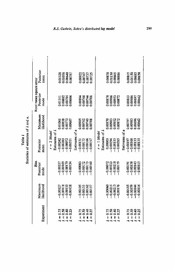
5. Some Monte Carlo results

Table 1 presents the results of some Monte Carlo experiments comparing the modes and means of the posterior distributions with the maximum likelihood estimates obtained from the procedure suggested by Maddala and Rao(1971). The experiments were conducted for various selected true values of 1 and the r = 2 and r = 1 models. a = 1.0 in all experiments. An experiment consisted

Tab

le

1

Sta

tist

ics

of e

stim

ates

of

A a

nd

a.

Exp

erim

ent

Max

imu

m

lik

elih

ood

Bia

s P

oste

rior

m

ode

L =

0.

75

A =

0.

50

I =

0.

40

1 =

0.

25

t =

0.

75

-0.0

0105

-0

.000

83

A =

0.

50

-0.0

0155

-0

.001

72

1. =

0.

40

-0.0

0162

-0

.001

73

A =

0.

25

-0.0

0157

-0

.001

60

-0.0

0127

-

0.00

337

-0.0

0118

-0

.001

69

-0.0

0153

-0

.001

79

-0.0

0128

-0

.001

34

Roo

t m

ean

squ

are

erro

r P

oste

rior

M

axim

um

P

oste

rior

P

oste

rior

m

ean

li

kel

ihoo

d m

ode

mea

n

r =

2

Mod

el

Est

imat

es

of 1

- 0.

0024

2 0.

0106

1 0.

0131

1 0.

0132

8 -

0.00

203

0.00

838

0.00

882

0.01

056

- 0.

0907

2 0.

0077

3 0.

0078

4 0.

0064

0 -0

.003

31

0.00

607

0.00

606

0.00

787

Est

imat

es

of a

-0.0

0131

0.

0090

5 0.

0089

4 0.

0092

2 -0

.001

73

0.00

762

0.00

768

0.00

767

-0.0

0166

0.

0074

0 0.

0074

4 0.

0073

7 -0

.001

97

0.00

708

0.00

708

0.00

725

1. =

0.

75

- 0.

0096

0 -

0.00

072

t =

0.

50

-0.0

0215

-

0.00

223

A =

0.

40

-0.0

0213

-0

.002

18

A 5

: 0.

25

-0.0

0176

-0

.001

79

,I =

0.

75

-0.0

0185

-0

.001

91

3. =

0.

50

-0.0

0159

-0

.001

58

A =

0.

40

-0.0

0144

-0

.001

43

A =

0.

25

-0.0

0116

-0

.001

15

r =

1

Mod

el

Est

imat

es

of 1

0.00

003

0.00

870

- 0.

0029

4 0.

0098

3 -0

.001

55

0.00

952

-0.0

0285

0.

0087

2

Est

imat

es

of a

-0.0

0197

0.

0079

7 -0

.001

68

0.00

983

-0.0

0133

0.

0069

6 -0

.001

35

0.00

662

0.00

878

0.00

878

0.00

986

0.01

150

0.00

953

0.00

805

0.00

872

0.00

886

0.00

813

0.00

815

0.00

986

0.01

150

0.00

697

0.00

685

0.00

662

0.00

658

300 R.S. Guihrie, Soiow’s distributed lag model

of 50 replications of samples of size 50. The data generated conformed with the assumptions of the model with X, a fixed sample of pseudorandom numbers rectangularly distributed over the interval from zero to 100. The disturbances were drawn from a normal distribution with zero mean and e,” = 4.0.

The bias statistics show that all three point estimators of 1 and a have very small biases. The root mean square error statistics are similar for the maximum likelihood and the two Bayesian point estimates. The RMSE values are very close for the maximum likelihood estimates and the modes of the posterior distributions.

References

Chetty, V.K., 1971, Estimation of Solow’s distributed lag models, Econometrica 39,99-l 17. Frazer, R.A., W.J. Duncan and A.R. Collar, 1938, Elementary matrices (Cambridge Univer-

sity Press, Cambridge, Mass.). Jeffreys, H., 1961, Theory of probability (Clarendon Press, Oxford). Maddala, G.S. and A.S. Rao, 1971, Solow’s and Jorgenson’s distributed lag models, The

Review of Economics and Statistics 53, 80-88. Schmidt, P., 1973, On the difference between conditional and unconditional asymptotic

distributions of estimates in distributed lag models with integer-valued parameters, Econo- metrica41,165-169.

Schmidt, P., 1974, An argument for the usefulness of the gamma distributed lag model, International Economic Review 15,246250.

Solow, R.M., 1960, On a family of lag distributions, Econometrica 28,393-406. Zcllner, A., 1971, An introduction to Bayesian inference in econometrics (Wiley, New York). Zellner, A. and M.S. Geisel, 1970, Analysis of distributed lag models with applications to

consumption function estimation, Econometrica 38,865-888.