CFD MODELING AND SIMULATION IN MATERIALS PROCESSING

A Parallel Cellular Automata Lattice Boltzmann Methodfor Convection-Driven Solidification

ANDREW KAO ,1,3 IVARS KRASTINS,1 MATTHAIOS ALEXANDRAKIS,1

NATALIA SHEVCHENKO,2 SVEN ECKERT,2 and KOULIS PERICLEOUS1

1.—Centre for Numerical Modelling and Process Analysis, University of Greenwich, Old RoyalNaval College, Park Row, London SE109LS, UK. 2.—Institute of Fluid Dynamics, Helmholtz-Zentrum Dresden-Rossendorf, Bautzner Landstrasse 400, 01328 Dresden, Germany. 3.—e-mail:a.kao@greenwich.ac.uk

This article presents a novel coupling of numerical techniques that enablethree-dimensional convection-driven microstructure simulations to be con-ducted on practical time scales appropriate for small-size components orexperiments. On the microstructure side, the cellular automata method isefficient for relatively large-scale simulations, while the lattice Boltzmannmethod provides one of the fastest transient computational fluid dynamicssolvers. Both of these methods have been parallelized and coupled in a singlecode, allowing resolution of large-scale convection-driven solidification prob-lems. The numerical model is validated against benchmark cases, extended tocapture solute plumes in directional solidification and finally used to modelalloy solidification of an entire differentially heated cavity capturing bothmicrostructural and meso-/macroscale phenomena.

INTRODUCTION

With increasing parallel computational power,microstructure modeling now has the capability toreach meso- or even macroscale dimensions. Inpractice, this means a single simulation cansimultaneously examine both micro- and macro-scale phenomena and their various interactions.In many cases, this removes the need for bound-ary condition approximations as the computationaldomain can encompass entire components orexperiments. To bridge the gap in scales, rangingfrom dendritic O(0.1 mm–1 mm) to componentO(1–10 cm), there are two key approaches. Thefirst is the operating length scale of the numericalmethods, which to achieve this goal should be thelargest for capturing microscopic phenomena. Thesecond is parallelization, which provided themethod scales well with increasing processersallows for increased domain sizes. On a practicallevel though, simulating a very large number ofcomputational cells is restricted to large high-performance computing clusters. The aim here isto combine these two approaches to allow timelysimulations of small-scale components orexperiments.

The phase field method is arguably the mostaccurate microstructural approach. Several investi-gators have parallelized this and modeled cases usingbillions of calculation cells. Takaki et al.1 used 64billion cells (40963) to simulate solidification withoutconvection in a 3:072 � 3:078 � 3:072-mm domain.Shimokawabe et al.2 developed a hybrid-parallelizedphase field method that uses the Message PassingInterface (MPI) and CUDATM. By using 16,000central processing unit (CPU) cores and 4000 graph-ical processing units (GPU), they achieved a compu-tational domain of 277 billion cells with a physicalsize of 3:072 � 4:875 � 7:8 mm3. Sakane et al.3 devel-oped a GPU parallelized lattice Boltzmann phasefield method and simulated 7 billion mesh points,with a real size of 61:5 � 61:5 � 123 lm3, using 512GPUs. Choudhury et al.4 compared a parallel cellularautomata method with a parallel phase field method,showing that the cellular automata method wasfaster in comparable 3D free undercooled growth.Similar success has been achieved with a 3D parallellattice Boltzmann cellular automata method5 simu-lating solute-driven multi-dendritic growth. By using6400 cores they simulated a domain of 36 billion cellswith a volume of 1 mm3.

JOM, Vol. 71, No. 1, 2019

https://doi.org/10.1007/s11837-018-3195-3� 2018 The Author(s)

48 (Published online November 12, 2018)

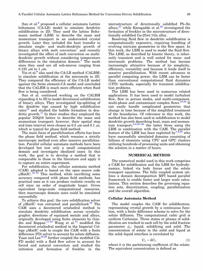
Sun et al.6 proposed a cellular automata Latticeboltzmann (CA-LB) model to simulate dendriticsolidification in 2D. They used the lattice Boltz-mann method (LBM) to describe the mass andmomentum transport in an undercooled crystalgrowth. Later they included the heat transfer tosimulate single- and multi-dendritic growth ofbinary alloys with melt convection7 and recentlyinvestigated the effect of melt convection on multi-dendritic growth without considering temperaturedifferences in the simulation domain.8 The meshsizes they used are all sub-micron ranging from0.125 lm to 1 lm.

Yin et al.9 also used the CA-LB method (CALBM)to simulate solidification at the microscale in 2D.They compared the efficiency of the CA-LB modelagainst the finite element-CA model and concludedthat the CALBM is much more efficient when fluidflow is being considered.

Sun et al. continued working on the CALBMexpanding it to 3D to model directional solidificationof binary alloys. They investigated tip-splitting ofthe dendrite tips caused by high solidificationrates10 and studied the bubble formation in den-dritic growth.11 In their studies they employed thepopular D3Q19 lattice to describe the mass andmomentum transport; however, their spatial stepand time interval were chosen as 0.5 lm and 0.1 ls,which is typical for phase field method.

The main focus of parallelization efforts has beenthe phase field method, which remains a strictlymicroscopic method even after massive paralleliza-tion. Parallel cellular automata methods have beendeveloped but test only a small computationaldomain and investigate idealized cases. In thiswork, the goal is to develop a method that iscomparable to those in the literature and apply itto capture an entire experiment.

For solidification, the cellular automata method(CAM) adopted is based on the open source codelMatIC.12–15 This method, while sacrificing someaccuracy compared with phase field methods, haspractical uses as it can produce realistic results oncell sizes an order of magnitude larger. Givenequivalent large-scale computational resources,then macroscopic domain sizes could be simulatedsuccessfully.

To achieve this goal, the core solidification solverof lMatIC was extracted and parallelized.16 TheCAM uses a decentered octahedral method tosimulate dendritic solidification across crystallo-graphic directions of equiaxed metals and alloys,originally developed using finite elements by Gan-din and Rappaz.17,18 Wang et al.14 modified thedecentered octahedral method in the Imperial Col-lege lMatIC code to couple the CAM with a finitedifference (FD) solver to account for solute diffusion.Yuan and Lee19,20 further coupled the modified CA-FD model with a fluid flow solver to account forforced and natural convection and studied theinitiation and formation of freckles in the

microstructure of directionally solidified Pb–Snalloys,21 while Karagadde et al.22 investigated theformation of freckles in the microstructure of direc-tionally solidified Ga-25wt.%In alloy.

Resolving fluid flow in dendritic solidification iscomputationally expensive, requiring handling ofevolving intricate geometries in the flow space. Inthis work, the LBM is used to model the fluid flow.The LBM, as described by kinetic theory, is inher-ently transient and is well suited for meso- andmicroscale problems. The method has becomeincreasingly attractive because of its simplicity,efficiency, versatility and because it lends itself tomassive parallelization. With recent advances inparallel computing power, the LBM can be fasterthan conventional computational fluid dynamics(CFD) methods, especially for transient solidifica-tion problems.

The LBM has been used in numerous relatedapplications. It has been used to model turbulentflow, flow in porous media, and multi-component,multi-phase and contaminant complex flows.23,24 Itcan easily handle complicated geometries thatchange in time because of the simplified treatmentof the boundaries. Of relevance to this work, themethod has also been used in solidification to modeldendritic growth describing heat, mass and momen-tum transport,5,9,25–28 the latter three using theLBM in combination with the CAM. The parallelfeature of the LBM has been exploited by1,3,28 whohave successfully simulated domains consisting ofbillions of elements using CPU and GPU clustersutilizing hundreds of processing units and obtainingthe solution in a matter of hours.

NUMERICAL METHOD

The numerical model used in this work comprisesa CAM for solidification and the LBM for hydrody-namics, linked via body forces and the solutetransport equations. The fully coupled system uti-lizes a domain decomposition MPI based parallelframework to enable faster and larger scale calcu-lations. This section describes the governing equa-tion sets, discretization, coupling, parallelizationand the overall algorithm.

Cellular Automata Method

The model couples the CAM for solidification,representing crystal growth by a continuous func-tion, with a finite difference scheme to solve for thesolute diffusion. The computational cubic grid isuniform Cartesian. Three states or phases of solid-ification are tracked in each cell by the solid fractionparameter /s: liquid, solidifying and solid. Theconcentration of solute in the solid and liquid atthe solid–liquid interface is correlated by

Cs ¼ kCl; ð1Þwhere k is the partitioning coefficient of the solute.The equivalent concentration is defined as

A Parallel Cellular Automata Lattice Boltzmann Method for Convection-Driven Solidification 49

Ce ¼ /lCl þ /sCs: ð2ÞThe convective transport of the solute is governedby

@Ce

@tCAMþ u � rCl ¼ r � DerClð Þ; ð3Þ

where u is the flow velocity in the liquid, and De ¼/lDl þ k/sDs is the equivalent diffusion coefficient.Equation 3 is discretized in an explicit form anduses a hybrid approach for the advection diffusionterms. At the interface, where u ¼ 0, the solidfraction rate of change is given by

Cl 1 � kð Þ @/s

@tCAM¼ �r � DerClð Þ

þ 1 � 1 � kð Þ/s½ � @Cl

@tCAM: ð4Þ

The solution procedure is essentially a loopbetween Eqs. 3 and 4. Convective transport iscalculated throughout the entire domain, and thenfrom local changes at the interface /s is updatedbased on transport and partitioning by Eq. 4. Equa-tions 3 and 4 determine the rate of solidification,but do not encapsulate any information on crystal-lographic orientation. This is handled by a decen-tered octahedral method, which essentiallyintroduces a bias for seeding neighboring cells tobegin solidifying. This bias corresponds to theunderlying crystallographic orientation, such thatcells along the direction of preferential growth willbe seeded first. This is calculated by considering thediagonal length of a rotated octahedron growing ineach cell. When this diagonal intersects a neighbor-ing cell, the neighbor is seeded with the sameunderlying orientation and begins to solidify. TheCAM used in this work is based on the lMatIC code,and through the parallelization and coupling pro-cess it was ensured that it gave the exact answerdown to machine precision. Due to the high Lewisnumber and low thermal Peclet number in the casesconsidered, a frozen thermal field approximation isused, where the temperature is explicitly knownboth spatially and temporally throughout thedomain. In this work the focus is on buoyancy-driven flow, which is applied in the liquid as

F ¼ qg 1 þ bT T � T0ð Þ þ bC C� C0ð Þð Þ ð5Þ

where q is the density, g is acceleration due togravity, bT and bC are the thermal and solutalexpansion coefficients, and T0 and C0 are a refer-ence temperature and concentration.

Lattice Boltzmann Method

The LBM is formulated using non-dimensionallattice Boltzmann units, where the lattice spacing,time stepping and equilibrium density are alldefined as unity. Therefore, all variables describedin this section are presented in a non-dimensionalform and for clarity those that have an equivalent

dimensioned form in the fully coupled method aredenoted with the superscript *. Scaling factors arederived from the real base SI units to scale betweenreal and dimensionless variables, for example, u� ¼u � DtLBM=DxLBM and the dimensionless forceF� ¼ FDt2LBM=qDxLBM. The LBM uses a discretizedfrom of the Boltzmann equation that describes theevolution of a particle distribution function (PDF),fi. The lattice Boltzmann equation is then given by

fi x� þ ciDt�LBM; t� þ Dt�LBM

� �� fi x�; t�ð Þ

¼ � 1

sfi � f eq

i

� �þ Dt�LBMF�

i ; ð6Þ

where the left-hand side represents the streamingprocesses, which govern the propagation of infor-mation to the neighboring cells. The right-hand sidedescribes collisions or the PDF relaxation towardsthe local equilibrium f eq

i in time s with an externalforce F�

i acting on the system. The equilibrium PDFf eqi is defined as

f eqi ¼ q�wi 1 þ ci � u�

c2s

þ ci � u�ð Þ2

2c4s

� u�2

2c2s

!

; ð7Þ

where q� is the fluid density, wi is the lattice weightcoefficient, ci is a discrete lattice velocity, cs is thespeed of sound, and u� is the fluid velocity. Todescribe the external forces such as thermo-solutalbuoyancy forces in this work, the HSD forcingscheme, named after the authors of Ref. 29 is usedand given by

F�i ¼ 1 � 1

2s

� �ci � u�ð Þ

c2s

� F�

mf eqi : ð8Þ

where m is the mass. A D3Q19 lattice is used in thecalculations with c2

s ¼ 13, the lattice weights wi are

given by

wi ¼1=3 i ¼ 01=18 i ¼ 1 . . . 61=36 i ¼ 7 . . . 18

8<

:ð9Þ

and the set of discrete lattice velocities for the modelcan be written as

ci ¼0; 0; 0ð Þ i ¼ 0�1; 0; 0ð Þ; 0;�1; 0ð Þ; 0; 0;�1ð Þ i ¼ 1 . . . 6�1;�1; 0ð Þ; 0;�1;�1ð Þ; �1; 0;�1ð Þ i ¼ 7 . . . 18

8<

:

ð10ÞFluid properties, such as density and fluid veloci-ties, can be calculated from the PDF by taking thevelocity moments as

q� ¼P

i

fi; q�u� ¼P

i

fici þ Dt�LBM

2F�: ð11Þ

The incompressible Navier–Stokes equations givenby

r � u� ¼ 0; ð12Þ

Kao, Krastins, Alexandrakis, Shevchenko, Eckert, and Pericleous50

@u�

@tþ u� � ru� ¼ � 1

q�rpþ m�r2u� þ F�; ð13Þ

can be recovered in the low Mach number limit atsmall velocities by following the Chapman–Enskogmultiscale analysis from (6), leading to the pressurep and the kinematic viscosity m� to be expressed as

p ¼ q�c2s ; ð14Þ

m� ¼ c2s s� 1

2

� �Dt�LBM: ð15Þ

For stability purposes, the two-relaxation-time(TRT) collision scheme is used. The TRT uses tworelaxation rates. One is directly linked to theviscosity of the physical system, while the other isa free parameter that can be fine-tuned for optimalaccuracy and stability.30–32

An extension of the 2D moment-based boundarymethod33–38 to 3D is used on the flat domainboundaries. The modified bounce-back rule, whichis second order accurate,39 is used for interiorboundaries.

Parallelization

Both the CAM and LBM are parallelized usingdomain decomposition with a boundary layer onecell wide for each process acting as a halo region toaccommodate MPI-based inter-processor communi-cation. Each process solves an equal-size sub-do-main. For processes that contain domainboundaries, the boundary layer is populated withthe physical boundary condition, while the haloregions contain the information from neighboringprocesses. The algorithm is designed so that thehalo regions are updated when values from neigh-boring cells are required and have changed onneighboring processes. Due to the explicit nature ofboth the CAM and LBM, this data exchange can bereduced to one update of the halo regions per timestep within each method. Updates to the physicaldomain boundary conditions also take place at thesame time. The MPI routine begins by updating thex direction boundaries using an odd and evenapproach; all the odd processors send and receivevalues from their even east neighbor, then the even

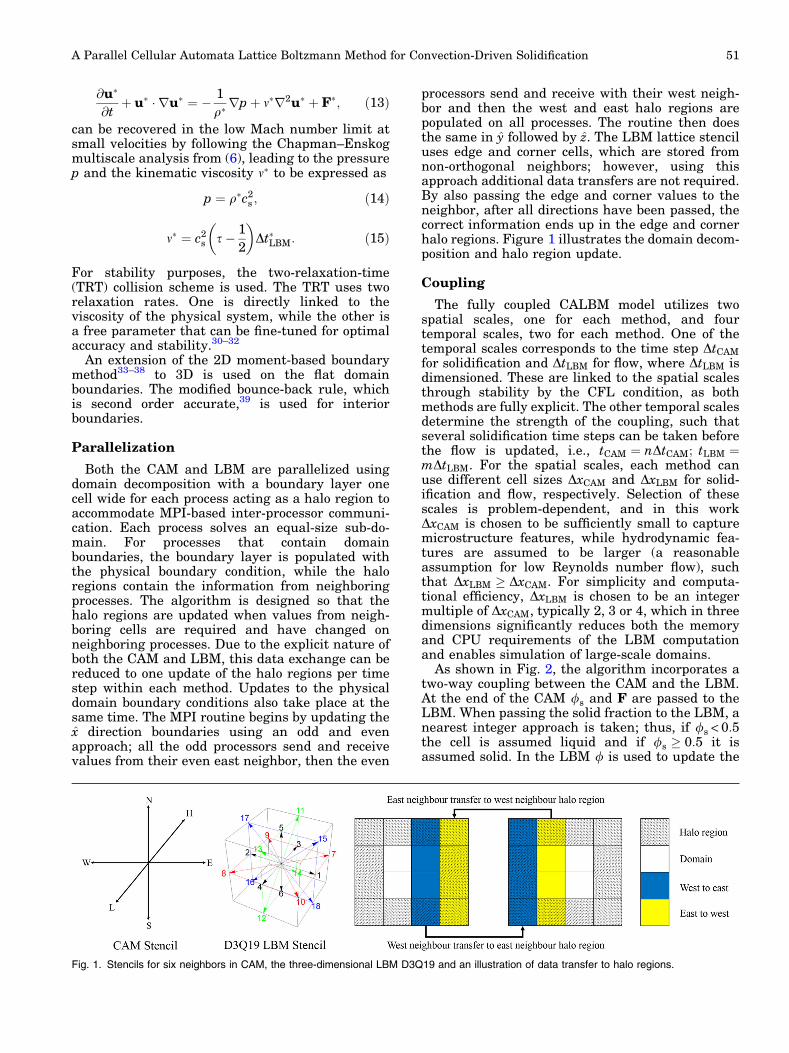
processors send and receive with their west neigh-bor and then the west and east halo regions arepopulated on all processes. The routine then doesthe same in y followed by z. The LBM lattice stenciluses edge and corner cells, which are stored fromnon-orthogonal neighbors; however, using thisapproach additional data transfers are not required.By also passing the edge and corner values to theneighbor, after all directions have been passed, thecorrect information ends up in the edge and cornerhalo regions. Figure 1 illustrates the domain decom-position and halo region update.

Coupling

The fully coupled CALBM model utilizes twospatial scales, one for each method, and fourtemporal scales, two for each method. One of thetemporal scales corresponds to the time step DtCAM

for solidification and DtLBM for flow, where DtLBM isdimensioned. These are linked to the spatial scalesthrough stability by the CFL condition, as bothmethods are fully explicit. The other temporal scalesdetermine the strength of the coupling, such thatseveral solidification time steps can be taken beforethe flow is updated, i.e., tCAM ¼ nDtCAM; tLBM ¼mDtLBM. For the spatial scales, each method canuse different cell sizes DxCAM and DxLBM for solid-ification and flow, respectively. Selection of thesescales is problem-dependent, and in this workDxCAM is chosen to be sufficiently small to capturemicrostructure features, while hydrodynamic fea-tures are assumed to be larger (a reasonableassumption for low Reynolds number flow), suchthat DxLBM � DxCAM. For simplicity and computa-tional efficiency, DxLBM is chosen to be an integermultiple of DxCAM, typically 2, 3 or 4, which in threedimensions significantly reduces both the memoryand CPU requirements of the LBM computationand enables simulation of large-scale domains.

As shown in Fig. 2, the algorithm incorporates atwo-way coupling between the CAM and the LBM.At the end of the CAM /s and F are passed to theLBM. When passing the solid fraction to the LBM, anearest integer approach is taken; thus, if /s < 0:5the cell is assumed liquid and if /s � 0:5 it isassumed solid. In the LBM / is used to update the

Fig. 1. Stencils for six neighbors in CAM, the three-dimensional LBM D3Q19 and an illustration of data transfer to halo regions.

A Parallel Cellular Automata Lattice Boltzmann Method for Convection-Driven Solidification 51

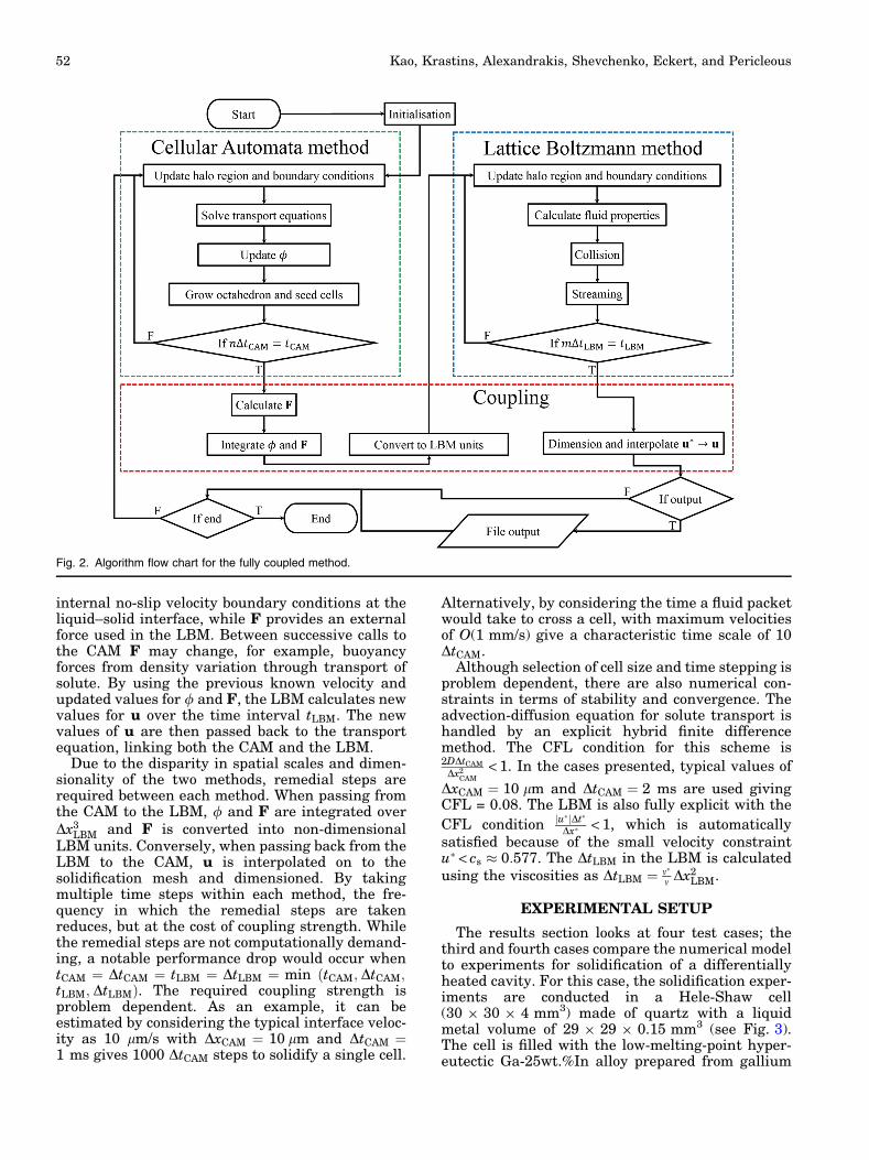
internal no-slip velocity boundary conditions at theliquid–solid interface, while F provides an externalforce used in the LBM. Between successive calls tothe CAM F may change, for example, buoyancyforces from density variation through transport ofsolute. By using the previous known velocity andupdated values for / and F, the LBM calculates newvalues for u over the time interval tLBM. The newvalues of u are then passed back to the transportequation, linking both the CAM and the LBM.

Due to the disparity in spatial scales and dimen-sionality of the two methods, remedial steps arerequired between each method. When passing fromthe CAM to the LBM, / and F are integrated overDx3

LBM and F is converted into non-dimensionalLBM units. Conversely, when passing back from theLBM to the CAM, u is interpolated on to thesolidification mesh and dimensioned. By takingmultiple time steps within each method, the fre-quency in which the remedial steps are takenreduces, but at the cost of coupling strength. Whilethe remedial steps are not computationally demand-ing, a notable performance drop would occur whentCAM ¼ DtCAM ¼ tLBM ¼ DtLBM ¼ min tCAM; DtCAM;ðtLBM; DtLBMÞ. The required coupling strength isproblem dependent. As an example, it can beestimated by considering the typical interface veloc-ity as 10 lm/s with DxCAM ¼ 10 lm and DtCAM ¼1 ms gives 1000 DtCAM steps to solidify a single cell.

Alternatively, by considering the time a fluid packetwould take to cross a cell, with maximum velocitiesof O(1 mm/s) give a characteristic time scale of 10DtCAM.

Although selection of cell size and time stepping isproblem dependent, there are also numerical con-straints in terms of stability and convergence. Theadvection-diffusion equation for solute transport ishandled by an explicit hybrid finite differencemethod. The CFL condition for this scheme is2DDtCAM

Dx2CAM

<1. In the cases presented, typical values of

DxCAM ¼ 10 lm and DtCAM ¼ 2 ms are used givingCFL = 0.08. The LBM is also fully explicit with the

CFL condition ju�jDt�Dx� <1, which is automatically

satisfied because of the small velocity constraintu� < cs 0:577. The DtLBM in the LBM is calculatedusing the viscosities as DtLBM ¼ m�

m Dx2LBM.

EXPERIMENTAL SETUP

The results section looks at four test cases; thethird and fourth cases compare the numerical modelto experiments for solidification of a differentiallyheated cavity. For this case, the solidification exper-iments are conducted in a Hele-Shaw cell(30 9 30 9 4 mm3) made of quartz with a liquidmetal volume of 29 9 29 9 0.15 mm3 (see Fig. 3).The cell is filled with the low-melting-point hyper-eutectic Ga-25wt.%In alloy prepared from gallium

Fig. 2. Algorithm flow chart for the fully coupled method.

Kao, Krastins, Alexandrakis, Shevchenko, Eckert, and Pericleous52

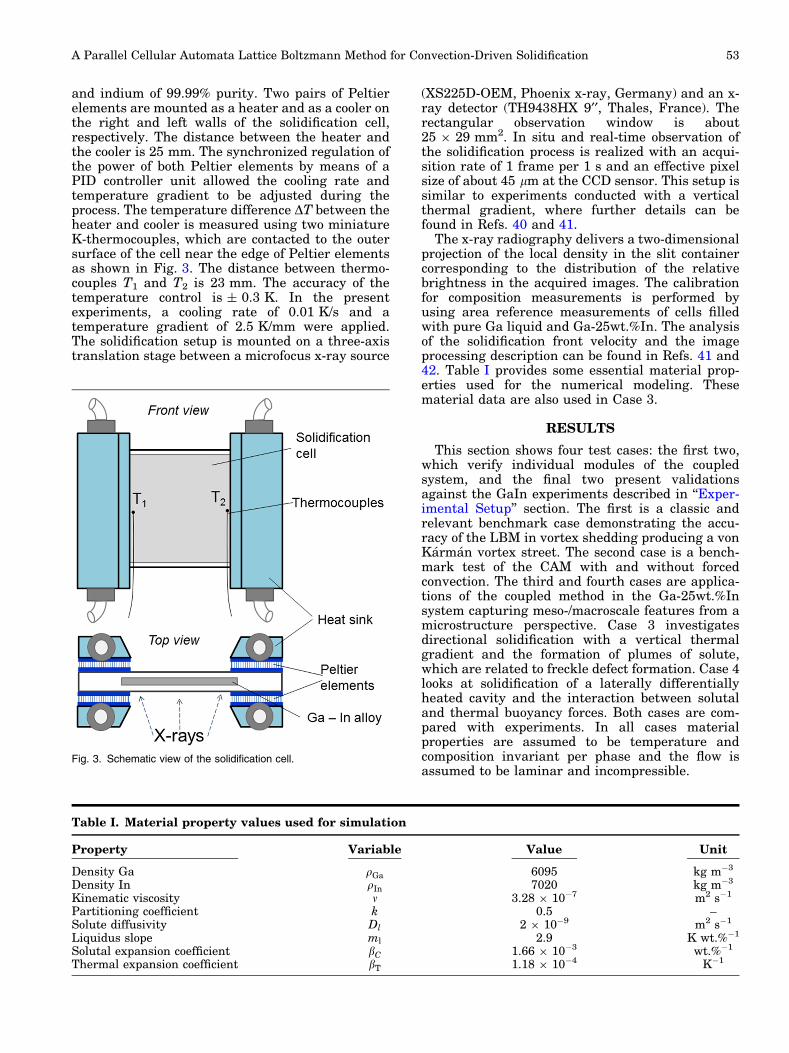
and indium of 99.99% purity. Two pairs of Peltierelements are mounted as a heater and as a cooler onthe right and left walls of the solidification cell,respectively. The distance between the heater andthe cooler is 25 mm. The synchronized regulation ofthe power of both Peltier elements by means of aPID controller unit allowed the cooling rate andtemperature gradient to be adjusted during theprocess. The temperature difference DT between theheater and cooler is measured using two miniatureK-thermocouples, which are contacted to the outersurface of the cell near the edge of Peltier elementsas shown in Fig. 3. The distance between thermo-couples T1 and T2 is 23 mm. The accuracy of thetemperature control is ± 0.3 K. In the presentexperiments, a cooling rate of 0.01 K/s and atemperature gradient of 2.5 K/mm were applied.The solidification setup is mounted on a three-axistranslation stage between a microfocus x-ray source

(XS225D-OEM, Phoenix x-ray, Germany) and an x-ray detector (TH9438HX 9¢¢, Thales, France). Therectangular observation window is about25 9 29 mm2. In situ and real-time observation ofthe solidification process is realized with an acqui-sition rate of 1 frame per 1 s and an effective pixelsize of about 45 lm at the CCD sensor. This setup issimilar to experiments conducted with a verticalthermal gradient, where further details can befound in Refs. 40 and 41.

The x-ray radiography delivers a two-dimensionalprojection of the local density in the slit containercorresponding to the distribution of the relativebrightness in the acquired images. The calibrationfor composition measurements is performed byusing area reference measurements of cells filledwith pure Ga liquid and Ga-25wt.%In. The analysisof the solidification front velocity and the imageprocessing description can be found in Refs. 41 and42. Table I provides some essential material prop-erties used for the numerical modeling. Thesematerial data are also used in Case 3.

RESULTS

This section shows four test cases: the first two,which verify individual modules of the coupledsystem, and the final two present validationsagainst the GaIn experiments described in ‘‘Exper-imental Setup’’ section. The first is a classic andrelevant benchmark case demonstrating the accu-racy of the LBM in vortex shedding producing a vonKarman vortex street. The second case is a bench-mark test of the CAM with and without forcedconvection. The third and fourth cases are applica-tions of the coupled method in the Ga-25wt.%Insystem capturing meso-/macroscale features from amicrostructure perspective. Case 3 investigatesdirectional solidification with a vertical thermalgradient and the formation of plumes of solute,which are related to freckle defect formation. Case 4looks at solidification of a laterally differentiallyheated cavity and the interaction between solutaland thermal buoyancy forces. Both cases are com-pared with experiments. In all cases materialproperties are assumed to be temperature andcomposition invariant per phase and the flow isassumed to be laminar and incompressible.

Fig. 3. Schematic view of the solidification cell.

Table I. Material property values used for simulation

Property Variable Value Unit

Density Ga qGa 6095 kg m�3

Density In qIn 7020 kg m�3

Kinematic viscosity m 3.28 9 10�7 m2 s�1

Partitioning coefficient k 0.5 –Solute diffusivity Dl 2 9 10�9 m2 s�1

Liquidus slope ml 2.9 K wt.%�1

Solutal expansion coefficient bC 1.66 9 10�3 wt.%�1

Thermal expansion coefficient bT 1.18 9 10�4 K�1

A Parallel Cellular Automata Lattice Boltzmann Method for Convection-Driven Solidification 53

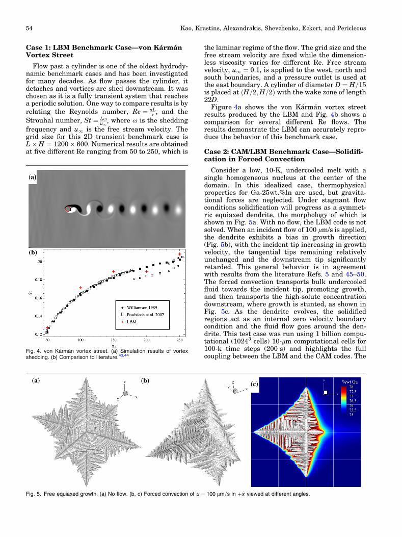
Case 1: LBM Benchmark Case—von KarmanVortex Street

Flow past a cylinder is one of the oldest hydrody-namic benchmark cases and has been investigatedfor many decades. As flow passes the cylinder, itdetaches and vortices are shed downstream. It waschosen as it is a fully transient system that reachesa periodic solution. One way to compare results is byrelating the Reynolds number, Re ¼ uL

m , and the

Strouhal number, St ¼ Lxu1

, where x is the shedding

frequency and u1 is the free stream velocity. Thegrid size for this 2D transient benchmark case isL�H ¼ 1200 � 600. Numerical results are obtainedat five different Re ranging from 50 to 250, which is

the laminar regime of the flow. The grid size and thefree stream velocity are fixed while the dimension-less viscosity varies for different Re. Free streamvelocity, u1 ¼ 0:1, is applied to the west, north andsouth boundaries, and a pressure outlet is used atthe east boundary. A cylinder of diameter D ¼ H=15is placed at H=2;H=2ð Þ with the wake zone of length22D.

Figure 4a shows the von Karman vortex streetresults produced by the LBM and Fig. 4b shows acomparison for several different Re flows. Theresults demonstrate the LBM can accurately repro-duce the behavior of this benchmark case.

Case 2: CAM/LBM Benchmark Case—Solidifi-cation in Forced Convection

Consider a low, 10-K, undercooled melt with asingle homogeneous nucleus at the center of thedomain. In this idealized case, thermophysicalproperties for Ga-25wt.%In are used, but gravita-tional forces are neglected. Under stagnant flowconditions solidification will progress as a symmet-ric equiaxed dendrite, the morphology of which isshown in Fig. 5a. With no flow, the LBM code is notsolved. When an incident flow of 100 lm/s is applied,the dendrite exhibits a bias in growth direction(Fig. 5b), with the incident tip increasing in growthvelocity, the tangential tips remaining relativelyunchanged and the downstream tip significantlyretarded. This general behavior is in agreementwith results from the literature Refs. 5 and 45–50.The forced convection transports bulk undercooledfluid towards the incident tip, promoting growth,and then transports the high-solute concentrationdownstream, where growth is stunted, as shown inFig. 5c. As the dendrite evolves, the solidifiedregions act as an internal zero velocity boundarycondition and the fluid flow goes around the den-drite. This test case was run using 1 billion compu-tational (10243 cells) 10-lm computational cells for100-k time steps (200 s) and highlights the fullcoupling between the LBM and the CAM codes. The

Fig. 4. von Karman vortex street. (a) Simulation results of vortexshedding. (b) Comparison to literature.43,44

Fig. 5. Free equiaxed growth. (a) No flow. (b, c) Forced convection of u ¼ 100 lm=s in þx viewed at different angles.

Kao, Krastins, Alexandrakis, Shevchenko, Eckert, and Pericleous54

boundary conditions for flow are a fixed velocity onthe west face, fixed pressure boundary for the eastface and zero Neumann conditions for the remain-ing faces.

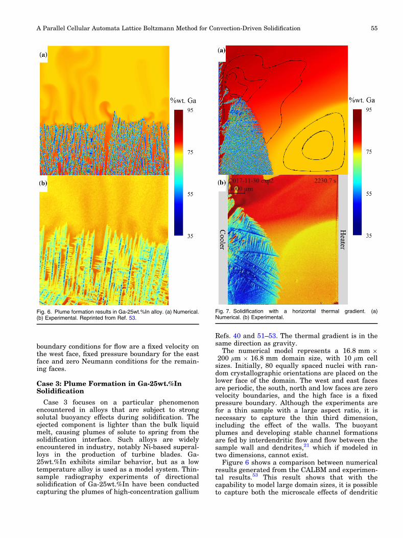
Case 3: Plume Formation in Ga-25wt.%InSolidification

Case 3 focuses on a particular phenomenonencountered in alloys that are subject to strongsolutal buoyancy effects during solidification. Theejected component is lighter than the bulk liquidmelt, causing plumes of solute to spring from thesolidification interface. Such alloys are widelyencountered in industry, notably Ni-based superal-loys in the production of turbine blades. Ga-25wt.%In exhibits similar behavior, but as a lowtemperature alloy is used as a model system. Thin-sample radiography experiments of directionalsolidification of Ga-25wt.%In have been conductedcapturing the plumes of high-concentration gallium

Refs. 40 and 51–53. The thermal gradient is in thesame direction as gravity.

The numerical model represents a 16.8 mm 9200 lm 9 16.8 mm domain size, with 10 lm cell

sizes. Initially, 80 equally spaced nuclei with ran-dom crystallographic orientations are placed on thelower face of the domain. The west and east facesare periodic, the south, north and low faces are zerovelocity boundaries, and the high face is a fixedpressure boundary. Although the experiments arefor a thin sample with a large aspect ratio, it isnecessary to capture the thin third dimension,including the effect of the walls. The buoyantplumes and developing stable channel formationsare fed by interdendritic flow and flow between thesample wall and dendrites,21 which if modeled intwo dimensions, cannot exist.

Figure 6 shows a comparison between numericalresults generated from the CALBM and experimen-tal results.53 This result shows that with thecapability to model large domain sizes, it is possibleto capture both the microscale effects of dendritic

Fig. 6. Plume formation results in Ga-25wt.%In alloy. (a) Numerical.(b) Experimental. Reprinted from Ref. 53.

Fig. 7. Solidification with a horizontal thermal gradient. (a)Numerical. (b) Experimental.

A Parallel Cellular Automata Lattice Boltzmann Method for Convection-Driven Solidification 55

growth and interdendritic flow with also themesoscale effects of interacting plumes and inter-acting grains in a single simulation from amicrostructure perspective. The numerical resultis taken after 1.8 million time steps (3600 s physicaltime). The domain tracks the interface such thatinformation is lost at the low face as solidificationprogresses and far field conditions are applied at thetop face. The simulation took 114 h on 120 cores.

Case 4: Ga-25wt.%In Solidification Subjectto a Horizontal Thermal Gradient

In this case, the domain is split into 3072 � 16 �3072 ¼ 151 million cells with Dx ¼ 9:375 lm. Thiscorresponds to a domain size of28:8 mm � 150 lm � 28:8 mm, closely representingthe full solidification experiment. In this case allboundaries are zero velocity representing the sam-ple walls. The domain is decomposed over 16 � 1 �8 ¼ 128 processors. Physical parameters includingthe thermal gradient and cooling rate are calibratedbased on experimental observations. Thirty-twonuclei with random crystallographic orientationsare equally distributed on the cold west wall of thedomain. Figure 7 shows a comparison between thenumerical model and the experimental results. Thenumerical result is taken at 2400 s (1.2 million timesteps) taking 72 h to compute, while the experimentis taken at 2230 s after the first dendrite isobserved. The slight disparity in time can beattributed to relatively large uncertainties in initialconditions. It is not possible to observe the nucle-ation events as they are covered by the cooler, and itis uncertain if there is any initial undercooling atnucleation. The results are in qualitatively goodagreement for both the interface shape and soluteconcentration profile.

With an initial homogeneous composition, fluidflow is dominated by thermal buoyancy forcesgenerating a counterclockwise rotating vortex witha direct analogy to a differentially heated cavity.However, as the system cools and solidificationprogresses, solute is ejected with increasing concen-tration. The strong but localized solute buoyancyforces overcome the thermal buoyancy force and asecondary vortex forms in the vicinity of the solid-ification front. Solute is transported to the top of thesample, stunting growth in this region. As moresolute is transported to the top surface of thesample, Ga-rich liquid extends across the top sur-face, forming a competing vortex and constrainingthe thermally driven vortex. As solidification pro-gresses further, a stable solute-rich channel forms,fed by interdendritic flow lower down the sample.This stable channel continues to feed the growingsolute-driven vortex. The solutal buoyancy-drivenvortex transports high-concentration Ga to theboundary of the two vortices, while the thermallydriven one drives the bulk concentration to theboundary. This leads to a stratification of

concentration, which is clearly visible in the exper-imental results. The overall mechanism is capturedby the numerical modeling; the location of thestable channel and the competing the vortices bothcompare favorably with the experimental observa-tions. This result demonstrates that the coupledCALBM has the capability to capture meso-macro-scale effects from a microstructural perspective; inthis case the entire experiment is modeled. Thisallows for direct modeling of constraints, for exam-ple, the sample end walls, where in many studiesonly sections of experiments can be captured andapproximate boundary conditions such as periodicor open boundaries are necessary, but may not berepresentative.

PERFORMANCE

In this section a summary of the performance ofthe various cases is given. In the cases presentedthe domain sizes vary from O(200 million to 1billion) cells. The parallel efficiency of the CALBMwas found to vary between 60% and 70%, asadditional computations are required for the inter-processor communication while updating the haloregions. The computational requirement of thesolvers scales with the cube of the domain length,while the communication scales as the square of thedomain length. Consequently, the higher efficiencycorresponds to the larger domain sizes. However,with increasing domain size per processor, the ratioof run time to simulated time increases. For exam-ple, case 4 took around 3 days to simulate 2400 s ofphysical time (1.2 million time steps). However, on asingle processor this would take an unfeasibleamount of time, around 270 days.

Case 2 provides a comparison of CAM and LBM.For free growth without flow the simulation took14 h to calculate 100-k CAM time steps, while withflow it took 19.5 h for the same number of steps.Approximately 2/3 of the simulation was resolvingsolidification; however, as DxLBM ¼ 4DxCAM thenumber of LBM cells was 64 times smaller. On aone-to-one scale, resolving the hydrodynamicswould take over 32 times longer than solidification,highlighting the necessity for variable length scalesbetween solidification and hydrodynamics. How-ever, as LBM has been shown to scale very wellwith GPUs, such approximations may be mitigatedin the future.

CONCLUSION

For simulating large-scale domains on amicrostructure scale that encompass small compo-nents or entire experimental setups, the coupledCALBM code has been shown to provide accurateresults at both the micro- and mesoscales. Each ofthe modules of the CALBM was validated againstclassic benchmark test cases. The LBM was shownto accurately predict the well-known relationshipbetween Re and St for low Re flow past a cylinder.

Kao, Krastins, Alexandrakis, Shevchenko, Eckert, and Pericleous56

The microstructure modeling was verified by simu-lation of a single free-growing equiaxed dendrite ina low-undercooled melt. Adding incident forcedconvection onto one of the dendrite arms, theCALBM was shown to give similar preferentialgrowth to results in the literature. The CALBM wasthen applied to two large-scale problems with bothmicro- and mesoscale features using the Ga-25wt.%In alloy. The first showed directional solid-ification with a vertical thermal gradient, where thegeneration of solute plumes due to solutal buoyancyled to the formation of solute channels in themicrostructure. The second investigated solidifica-tion of a differentially heated cavity with a horizon-tal thermal gradient, where a competition betweenthermal and solutal buoyancy forces led to twolarge-scale counter-rotating vortices. Ejected soluteis fed by the large solutal buoyancy force drivingflow in the interdendritic region. In both of thevalidation cases, favorable agreement at both themicro- and mesoscale was found between thenumerical and experimental results.

FUTURE WORK

The CAM and LBM were chosen for this work asthey represent potentially the largest microstruc-ture-length-scale computational tool and fastesttransient flow simulator respectively. They alsolend themselves to massive parallelization. In theexamples presented, parallelization was only con-ducted on a CPU over MPI basis. These methods,certainly LBM, can see huge speed increases whenutilizing GPUs. However, there will be an increasein communication overheads from transferring databetween the CPU and GPU of field data and to keepthe halo regions updated via MPI. Such GPUimplementations have been realized in other relatedmethods with a high degree of success, and as suchthey are worth pursuing for the CALBM. With theability to simulate O(1 billion) cells in a timelymanner, the entire microstructure of small compo-nents O(100 mm 9 100 mm 9 100 mm) could bereadily predicted. The results presented here pro-vide a qualitative agreement with the experimentalresults; however, with increasing cell size there willbe a loss of accuracy in capturing microstructuralfeatures, but this will allow for even larger domains.A future study is planned to quantify the behavior ofthis error. This will encompass a direct comparisonof solute concentration profiles between the numer-ical and experimental results.

ACKNOWLEDGEMENTS

Part of this study was funded by the UK Engi-neering and Physical Sciences Research Council(EPSRC) under Grant EP/K011413/1. M. Alexan-drakis and I. Krastins gratefully acknowledgefunding of their PhD studies under the University ofGreenwich Vice Chancellor postgraduate grantscheme.

OPEN ACCESS

This article is distributed under the terms of theCreative Commons Attribution 4.0 International Li-cense (http://creativecommons.org/licenses/by/4.0/),which permits unrestricted use, distribution, andreproduction in any medium, provided you give ap-propriate credit to the original author(s) and thesource, provide a link to the Creative Commons li-cense, and indicate if changes were made.

REFERENCES

1. T. Takaki, T. Shimokawabe, M. Ohno, A. Yamanaka, and T.Aoki, J. Cryst. Growth 382, 21 (2013).

2. T. Shimokawabe, T. Aoki, T. Takaki, T. Endo, A. Yamanaka,N. Maruyama, A. Nukada, and S. Matsuoka, Proceedings of2011 International Conference in High Performance Com-putation, p. 3 (2011).

3. S. Sakane, T. Takaki, R. Rojas, M. Ohno, Y. Shibuta, T.Shimokawabe, and T. Aoki, J. Cryst. Growth 474, 154(2017).

4. A. Choudhury, K. Reuther, E. Wesner, A. August, B. Nes-tler, and M. Rettenmayr, Comput. Mater. Sci. 55, 263 (2012).

5. M. Eshraghi, M. Hashemi, B. Jelinek, and S. Felicelli, Me-tals 7, 474 (2017).

6. D. Sun, M. Zhu, S. Pan, and D. Raabe, Acta Mater. 57, 1755(2009).

7. D. Sun, M. Zhu, S. Pan, C. Yang, and D. Raabe, Comput.Math. Appl. 61, 3585 (2011).

8. D. Sun, Y. Wang, H. Yu, and Q. Han, Int. J. Heat MassTransf. 123, 213 (2018).

9. H. Yin, S. Felicelli, and L. Wang, Acta Mater. 59, 3124(2011).

10. D. Sun, M. Zhu, J. Wang, and B. Sun, Int. J. Heat MassTransf. 94, 474 (2016).

11. D. Sun, S. Pan, Q. Han, and B. Sun, Int. J. Heat MassTransf. 103, 821 (2016).

12. P. Lee, R. Atwood, R. Dashwood, and H. Nagaumi, Mater.Sci. Eng. A 328, 213 (2002).

13. P. Lee, A. Chirazi, R. Atwood, and W. Wang, Mater. Sci.Eng. A 365, 57 (2004).

14. W. Wang, P. Lee, and M. Mclean, Acta Mater. 51, 2971(2003).

15. H. Dong and P. Lee, Acta Mater. 53, 659 (2005).16. M. Alexandrakis, Ph.D. Thesis, University of Greenwich

(2018).17. M. Rappaz and C. Gandin, Acta Metall. Mater. 41, 345

(1993).18. C. Gandin and M. Rappaz, Acta Mater. 45, 2187 (1997).19. L. Yuan, P. Lee, G. Djambazov, and K. Pericleous, Modeling

of Casting, Welding, and Advanced Solidification ProcessesXII, p. 451 (2010).

20. L. Yuan and P. Lee, Model. Simul. Mater. Sci. Eng. 18,55008 (2010).

21. L. Yuan and P. Lee, Acta Mater. 60, 4917 (2012).22. S. Karagadde, L. Yuan, N. Shevchenko, S. Eckert, and P.

Lee, Acta Mater. 79, 168 (2014).23. S. Chen and G. Doolen, Annu. Rev. Fluid Mech. 30, 329

(1998).24. C. Aidun and J. Clausen, Annu. Rev. Fluid Mech. 42, 439

(2010).25. W. Miller, S. Succi, and D. Mansutti, Phys. Rev. Lett. 86,

3578 (2001).26. D. Chatterjee and S. Chakraborty, Phys. Lett. A 351, 359

(2006).27. M. Eshraghi, S. Felicelli, and B. Jelinek, J. Cryst. Growth

354, 129 (2012).28. M. Eshraghi, B. Jelinek, and S. Felicelli, JOM 67, 1786

(2015).29. X. He, X. Shan, and G. Doolen, Phys. Rev. E 57, 13 (1998).30. I. Ginzburg, F. Verhaeghe, and D. d’Humieres, Commun.

Comput. Phys. 3, 427 (2008).

A Parallel Cellular Automata Lattice Boltzmann Method for Convection-Driven Solidification 57

31. I. Ginzburg, D. d’Humieres, and A. Kuzmin, J. Stat. Phys.139, 1090 (2010).

32. I. Ginzburg, Commun. Comput. Phys. 11, 1439 (2012).33. S. Bennett, P. Asinari, and P. Dellar, Int. J. Numer. Meth-

ods Fluids 69, 171 (2012).34. S. Bennett, Ph.D. Thesis, University of Cambridge (2010).35. T. Reis and P. Dellar, Phys. Fluids 24, 112001 (2012).36. A. Hantsch, T. Reis, and U. Gross, J. Comput. Multiph.

Flows 7, 1 (2015).37. R. Allen and T. Reis, Prog. Comput. Fluid Dyn. 16, 216

(2016).38. S. Mohammed and T. Reis, Arch. Mech. Eng. 64, 57 (2017).39. Z. Guo and C. Shu, Lattice Boltzmann Method and Its

Applications in Engineering, Vol. 3 (Singapore: World Sci-entific, 2013), p. 42.

40. N. Shevchenko, S. Boden, G. Gerbeth, and S. Eckert, Metall.Mater. Trans. A 44, 3797 (2013).

41. N. Shevchenko, O. Roshchupkina, O. Sokolova, and S.Eckert, J. Cryst. Growth 417, 1 (2015).

42. S. Boden, S. Eckert, B. Willers, and G. Gerbeth, Metall.Mater. Trans. A 39, 613 (2008).

43. C. Williamson, J. Fluid Mech. 206, 579 (1989).44. O. Posdziech and R. Grundmann, J. Fluids Struct. 23, 479

(2007).45. J. Jeong, N. Goldenfeld, and J. Dantzig, Phys. Rev. E 64,

41602 (2001).46. Y. Lu, C. Beckermann, and A. Karma, ASME’s International

Mechanical Engineering Congress and Exposition, p. 197(2002).

47. N. Al-Rawahi and G. Tryggvason, J. Comput. Phys. 194, 677(2004).

48. Y. Lu, C. Beckermann, and J. Ramirez, J. Cryst. Growth280, 320 (2005).

49. L. Tan and N. Zabaras, J. Comput. Phys. 211, 36 (2006).50. L. Tan and N. Zabaras, J. Comput. Phys. 221, 9 (2007).51. N. Shevchenko, S. Eckert, S. Boden, G. Gerbeth, and I.O.P.

Conf, Ser. Mater. Sci. Eng. 33, 12035 (2012).52. N. Shevchenko, S. Boden, S. Eckert, G. Gerbeth, and I.O.P.

Conf, Ser. Mater. Sci. Eng. 27, 12085 (2012).53. A. Kao, N. Shevchenko, O. Roshchupinka, S. Eckert, K.

Pericleous, and I.O.P. Conf, Ser. Mater. Sci. Eng. 84, 12018(2015).

Kao, Krastins, Alexandrakis, Shevchenko, Eckert, and Pericleous58