A Phillips Curve with Anchored Expectations and Short‐Term ...Keywords: inﬂation, Phillips curve. HOW DOES UNEMPLOYMENT AFFECT INFLATION?Thisquestionhas been a controversial topic

DOI: 10.1111/jmcb.12502

LAURENCE BALL

SANDEEP MAZUMDER

A Phillips Curve with Anchored Expectations and

Short-Term Unemployment

This paper examines the behavior of U.S. core inflation, as measured bythe weighted median of industry price changes. We find that core inflationsince 1985 is well-explained by an expectations-augmented Phillips curve inwhich expected inflation is measured with professional forecasts and labor-market slack is captured by the short-term unemployment rate. We alsofind that expected inflation was backward-looking until the late 1990s, butthen became strongly anchored at the Federal Reserve’s target. This shift inexpectations changed the relationship between inflation and unemploymentfrom an accelerationist Phillips curve to a level-level Phillips curve. Ourspecification explains why high unemployment during the Great Recessiondid not reduce inflation greatly: partly because inflation expectations wereanchored, and partly because short-term unemployment rose less sharplythan total unemployment.

JEL codes: E31Keywords: inflation, Phillips curve.

HOW DOES UNEMPLOYMENT AFFECT INFLATION? This question hasbeen a controversial topic in macroeconomics since Phillips (1958) and Samuelsonand Solow (1960). Since the Great Recession of 2008–9, economists have entered anew phase of research and debate about the unemployment-inflation relationship.

Recent research has been spurred by a puzzle: the “missing deflation” (Stock 2011).The accelerationist Phillips curve of textbooks says that a high level of unemploymentcauses inflation to fall over time. For common calibrations of this relationship, thehigh unemployment rates during the recession and subsequent weak recovery shouldhave pushed the inflation rate well below zero. Yet in recent years, the rate of core

We are grateful for research assistance from Emek Karaca and for suggestions from Robert Gordon,Kenneth West, David Romer, and an anonymous referee. We also thank Randall Verbrugge and ChristianGarciga for providing data.

LAURENCE BALL is at Department of Economics, Johns Hopkins University (E-mail: [email protected]).SANDEEP MAZUMDER is at Department of Economics, Wake Forest University (E-mail: [email protected]).

Received March 3, 2015; and accepted in revised form March 21, 2018.

Journal of Money, Credit and Banking, Vol. 00, No. 0 (xxxx 2018)C© 2018 The Ohio State University

2 : MONEY, CREDIT AND BANKING

inflation—inflation excluding the transitory effects of supply shocks—has been closeto its level before 2008. Many observers have concluded that “we don’t have a verygood story about inflation and unemployment these days” (Krugman 2014).

Many economists have proposed resolutions of the missing-deflation puzzle, andtwo basic ideas have become popular. The first idea, emphasized by Fed officials (e.g.,Bernanke 2010) and the IMF (2013), among others, is that inflation expectations havebecome anchored. According to this story, the Fed’s commitment to a 2% inflationtarget has kept expected inflation near 2%, which in turn has prevented actual inflationfrom falling very far below that level.

The second explanation, proposed by Stock and by Gordon (2013), is that inflationdepends not on the aggregate unemployment rate, as in textbook Phillips curves, butrather on the short-term unemployment rate. This variable is defined as the percentageof the labor force unemployed for 26 weeks or less. The story here is that the short-term unemployed put downward pressure on wages but the long-term unemployeddo not, because their attachment to the labor force is weak. This idea helps explainwhy inflation has not fallen by more, because short-term unemployment rose lesssharply than total unemployment over 2008–9, and then returned more quickly toprerecession levels.

Section 1 of this paper reviews the textbook Phillips curve and the puzzling behaviorof inflation since 2008. We also present informal evidence that this puzzle may beexplained by the behavior of expectations and of short-term unemployment.

In Section 2, we begin our econometric analysis of the behavior of core inflation.An important feature of our approach is that we measure core inflation with theweighted median of industry price changes, as constructed by the Federal ReserveBank of Cleveland. In our view, this core-inflation measure is preferable to moretraditional measures, such as inflation excluding food and energy prices, on boththeoretical and empirical grounds.

We seek to explain core-inflation behavior with a simple Phillips curve. FollowingFriedman (1968), we assume that core inflation depends on expected inflation and thelevel of unemployment, with the twist that only short-term unemployment matters.To estimate this equation, we measure expected inflation with long-term forecastsfrom the Survey of Professional Forecasters (SPF). Our Phillips curve fits the datawell from 1985 through 2015, with little evidence of instability during the GreatRecession or any other period.

Section 3 examines the behavior of inflation expectations as measured by the SPFforecasts. We assume that expected inflation is a weighted average of a backward-looking term—an average of past inflation rates—and a fixed inflation target. Here, wefind strong evidence of a regime shift in the late 1990s: the weight on the backward-looking term drops from approximately one to near zero. That is, expectations werefully backward-looking in the first part of our sample, but then became stronglyanchored.

Section 4 again considers an expectations-augmented Phillips curve, but insteadof measuring expected inflation directly we use our assumption that this variable isa mixture of a backward-looking term and a fixed target. Estimates of this equation

LAURENCE BALL AND SANDEEP MAZUMDER : 3

are consistent with our other results: the effect of short-term unemployment oninflation appears to be constant, but the effect of past inflation falls sharply in thelate 1990s. Overall, the data suggest a stable expectations-augmented Phillips curvewith short-term unemployment, but a shift in the reduced-form relationship betweenunemployment and inflation resulting from the anchoring of expectations.

Section 5 returns to the motivation for our research, the missing deflation since2008. We find that this anomaly disappears with our preferred specification of thePhillips curve.

Section 6 presents a caveat to our results: they weaken considerably if we changeour measure of core inflation from weighted median inflation to inflation excludingfood and energy prices. Section 7 concludes the paper and emphasizes another caveat:our success at explaining recent inflation behavior partly reflects the fact that ourPhillips curve is designed for that purpose. Going forward, new data will allow us tojudge how well our specification fits inflation behavior in general.

1. RECENT THINKING ABOUT THE PHILLIPS CURVE

Here we review the textbook Phillips curve, the puzzle of the missing deflation,and recent discussions of expectations anchoring and short-term unemployment.

1.1 The Phillips Curve and the Missing Deflation

In his Presidential Address to the American Economic Association, Friedman(1968) posited that the inflation rate depends on expected inflation and the deviationof unemployment from its natural rate. Friedman’s theory can be expressed as

πt = π et + α

(ut − u∗

t

) + εt , α < 0, (1)

where πt is inflation, π et is expected inflation, ut is unemployment, u∗

t is the naturalrate, and εt is an error term. This equation is commonly called the expectations-augmented Phillips curve.

Friedman went a step further by specifying the behavior of expectations. He saidthat “unanticipated inflation generally means a rising rate of inflation,” or in otherwords, that expected inflation is well-proxied by past inflation. With this assumption,equation (1) becomes

πt = πt−1 + α(ut − u∗

t

) + εt , (2)

where πt−1 is past inflation. This equation is the accelerationist Phillips curve, astaple of undergraduate textbooks. It is often written with past inflation moved to left:

πt − πt−1 = α(ut − u∗

t

) + εt . (3)


As we see here, the textbook Phillips curve is a negative relationship between thelevel of unemployment and the change in inflation.

Equation (2) has guided much empirical research on U.S. inflation, including thework of Gordon (1982, 2013), Stock and Watson (1999, 2009), Ball and Mazumder(2011), and many others. Typically these researchers seek to explain quarterly dataon core inflation, capturing past core inflation with four or more lags. Their equationsoften include lags of unemployment as well, and allow the natural rate u∗

t to varyover time.

As Stock and Watson (2010) discuss, the accelerationist Phillips curve has hadenduring appeal because it captures “a broad historical regularity”: since 1960, U.S.recessions have led to decreases in the inflation rate. The most salient example is therecession of the early 1980s, which pushed the unemployment rate above 10%. Inthis episode, core inflation fell by about 6 percentage points.

This history explains why recent inflation behavior has puzzled economists. Duringthe Great Recession of 2008–9, the unemployment rate again exceeded 10%, and itreturned to prerecession levels only at the end of 2015. Therefore, as shown formallybelow, an accelerationist Phillips curve that once fit the data predicts that inflationfalls below zero in late 2010 and then continues to fall. In reality, from 2007Q4to 2015Q4, the four-quarter rate of core inflation fell only from 2.3% to 2.0% ifmeasured by the CPI excluding food and energy, and from 3.0% to 2.3% for medianCPI. The disinflationary effect of recessions—“the essential empirical content of thePhillips curve,” according to Stock and Watson—seems to have disappeared.1

1.2 Anchored Expectations

Why has inflation not fallen by more? Many policymakers and economists cite theanchoring of inflation expectations. For example, according to Janet Yellen (2013):

Well-anchored inflation expectations have proven to be an immense asset in conductingmonetary policy. They’ve helped keep inflation low and stable while monetary policyhas been used to help promote a healthy economy. After the onset of the financial crisis,these stable expectations also helped the United States avoid excessive disinflation oreven deflation.

According to this story, the expectations-augmented Phillips curve, equation (1),still holds, but the behavior of expectations has changed. In the past, expected inflationπ e

t may have depended on lagged inflation, but today it is close to a constant—specifically, the Fed’s 2% inflation target. With a constant π e

t , the Phillips curvebecomes a relationship between unemployment and the level of inflation, not thechange in inflation.

1. As the reader probably knows, much academic research has analyzed the “New Keynesian” Phillipscurve (NKPC), in which inflation depends on expected future inflation and real marginal cost (e.g., Galı́2008). The empirical validity of the NKPC is disputed, and we are on the side that believes it does not fitinflation behavior in general or recent U.S. inflation in particular. We discuss this issue in our 2011 paper(Section 5), and have nothing to add here.


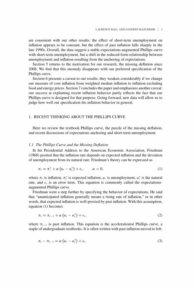
FIG. 1. Long-Term SPF Inflation Expectations versus Four-Quarter Moving Average of Median Inflation, 1985–2015.

This idea goes in the right direction for explaining the missing deflation. Accordingto the accelerationist Phillips curve, a recession causes inflation to fall lower and loweras long as unemployment exceeds the natural rate. With anchored expectations, aperiod of high unemployment implies a low level of inflation but not an ever-fallinglevel.

The idea of anchored expectations predates the Great Recession. The Fed an-nounced a formal inflation goal of 2% only in 2012, but research as far back as Taylor(1993) finds that the Fed was implicitly targeting 2%. In the 2000s, Fed officialsbegan to suggest that their commitment to stable inflation “in both words and ac-tions” had produced “a strong anchoring of long-run inflation expectations” (Mishkin2007).

An important detail: The Fed’s target of 2% applies to inflation as measured bythe PCE (personal consumption expenditure) deflator excluding food and energy.Since 1980, this measure of core PCE inflation has averaged about 0.5% less thancore CPI inflation (for both the weighted-median and ex-food-and-energy measuresof core CPI). We should expect, therefore, that expectations of core CPI inflation areanchored at a level near 2.5%.

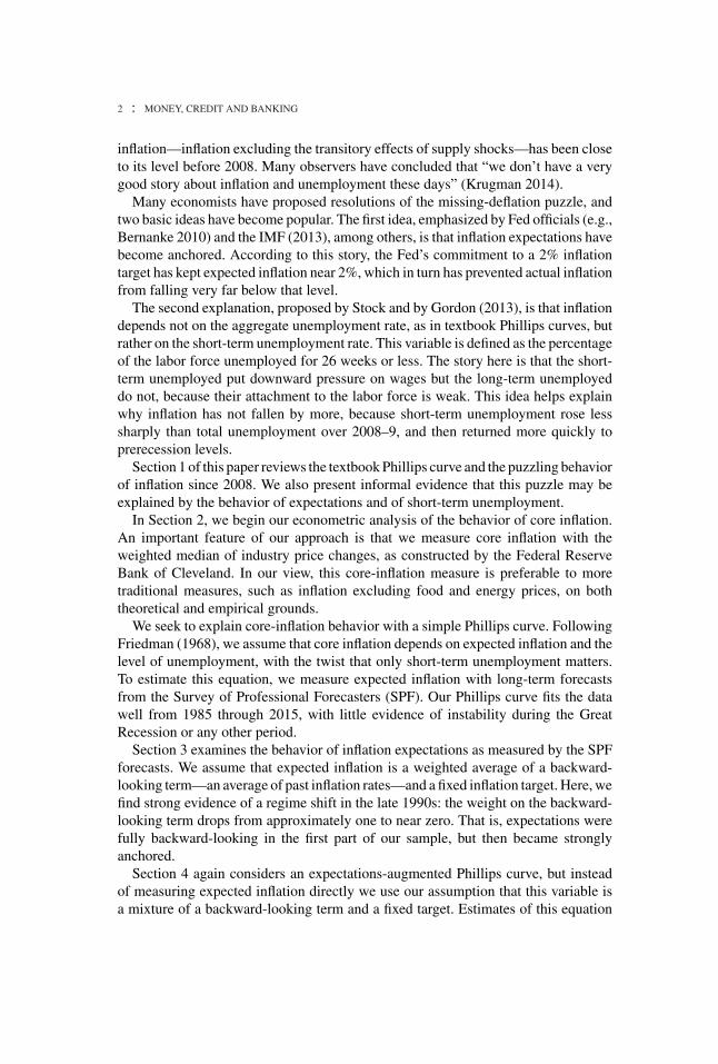
As many researchers have pointed out, the idea of anchored expectations receivesstriking support from long-term inflation forecasts in the SPF. For the period from1985 through 2015, Figure 1 shows the mean SPF forecast of CPI inflation overthe next 10 years, along with a four-quarter moving average of weighted medianinflation. From 1985 until the late 1990s, SPF forecasts drift down along with the


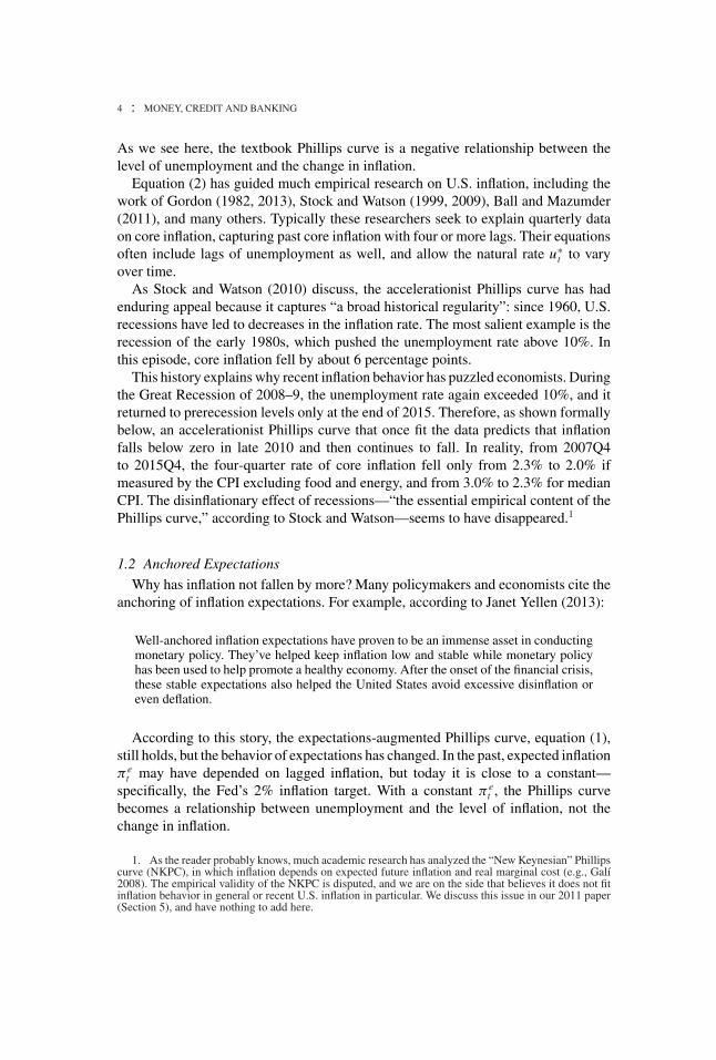
FIG. 2. Short-Term Unemployment versus Total Unemployment, 1985–2015.

realized levels of median inflation. Since the late 1990s, by contrast, SPF forecastsare almost constant at 2.5%, despite significant fluctuations in median inflation.

1.3 Short-Term Unemployment

The traditional Phillips curve includes the aggregate unemployment rate. A grow-ing number of researchers replace this variable with the short-term unemploymentrate—usually defined as the percentage of the labor force unemployed for less than27 weeks—and argue that this modification helps explain the missing deflation.

The rationale for this specification is that the long-term unemployed “are on themargins of the labor force” (Krueger, Cramer, and Cho 2014). These workers areunlikely to find jobs because they are unattractive to employers and because theydo not search intensively for work. As a result, only the short-term unemployedcreate an excess supply of labor and put downward pressure on wage growth andinflation.

Figure 2 shows how this reasoning helps explain the missing deflation. Long-termunemployment rose sharply over 2008–9, so the rise in total unemployment wasunusually large compared to the rise in short-term unemployment. Long-term unem-ployment has continued to be unusually high relative to short-term unemploymenteven as total unemployment has returned to prerecession levels. Overall, labor-marketslack since 2008 is less severe if it is measured by short-term rather than total unem-ployment, so the Phillips curve predicts a smaller fall in inflation in this case.


Phillips curves with short-term unemployment were introduced in the 1980s toexplain experiences in Europe, where inflation rates were stable despite high long-term unemployment (e.g., Nickell 1987). Llaudes (2005) shows that this Phillips-curve specification fits the data for a number of countries.

Before the Great Recession, students of the U.S. Phillips curve rarely consideredspecifications with short-term unemployment. The reason is that short-term and totalunemployment were highly collinear in U.S. data, making it difficult to separatetheir effects (as shown formally below). This collinearity problem has diminishedsubstantially since 2008 because of the disproportionate rise in total unemployment.

2. AN EXPECTATIONS-AUGMENTED PHILLIPS CURVE

In our econometric work, we seek to explain the behavior of core inflation from1985 through 2015. During this period, the level and volatility of inflation were fairlylow, making it plausible that a stable Phillips curve fits the data. We do not examine the1970s or early 1980s, when high and volatile inflation produced a different Phillipscurve. (In particular, both theory and evidence suggest that changes in unemploymenthad larger effects on inflation before 1985; see Ball and Mazumder 2011).

In this section, we examine a Phillips curve in which core inflation is measuredby the weighted median inflation rate; expected inflation is measured with forecastsfrom the SPF; and economic slack is measured with short-term unemployment. Thisequation fits the data well throughout the 1985–2015 period.

2.1 Measuring Core Inflation

The most common measure of core inflation is the growth rate of the price level(either the CPI or the PCE deflator) excluding food and energy prices. We choose,however, to use the weighted median of industry inflation rates, as constructed bythe Federal Reserve Bank of Cleveland.2 We will see that our results are not ro-bust to measuring core inflation in the traditional way, but that finding does nottrouble us greatly because we believe the weighted median is a better core-inflationmeasure.

As we discuss in Ball and Mazumder (2011), the weighted median is a good core-inflation measure because it filters out movements in headline inflation caused bylarge relative-price changes in any industry, not just food and energy. Our earlierpaper finds that, since 2000, quarterly innovations in median inflation have beenalmost entirely permanent, whereas inflation in the CPI excluding food and energy(CPIX) has a substantial transitory component. Median inflation does a better job ofcapturing the underlying trend in inflation.

2. As in Ball and Mazumder (2011), we compute a quarterly series for weighted median inflation fromthe monthly series reported by the Cleveland Fed. We first cumulate the monthly median inflation rates toconstruct a monthly series for price levels, then average 3 months to get quarterly price levels. Quarterlymedian inflation is the annualized percentage change in the quarterly price level.


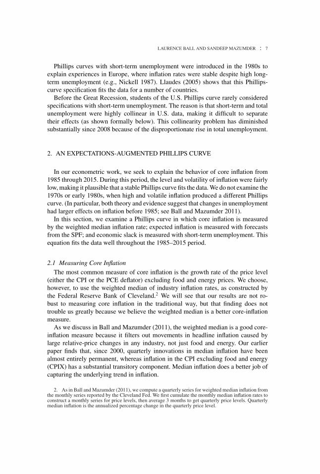
FIG. 3. Median CPI and CPIX Quarterly Inflation, 2000–15.

Figure 3 illustrates the appeal of the weighted median by plotting this variable andCPIX inflation over 2000–15. We can see that CPIX inflation is more volatile at thequarterly frequency. The standard deviation of the change in inflation is 0.44 for themedian and 0.64 for CPIX.

2.2 Specification

We consider a version of Friedman’s expectations-augmented Phillips curve,equation (1), in which labor-market slack is measured by the deviation of short-termunemployment from its natural rate. Following Staiger, Stock, and Watson (1997)and Gordon (2013), we specify an equation for quarterly data with four lags of theunemployment term:

πt = π et +

4∑

j=1

α j(us

t− j − us∗t− j

) + εt , (4)

where πt is the annualized rate of core inflation, π et is expected inflation, us

is the short-term unemployment rate, and us∗ is the natural rate of short-termunemployment.

For parsimony, we assume that the coefficients on the four unemployment lags areequal, that is, that inflation depends on average short-term unemployment over theprevious four quarters. When we test this restriction, it is not rejected (p-value forWald test = 0.53). We can now write equation (4) as

πt = π et + α

(us

t−1 − us∗t−1

) + εt , (5)


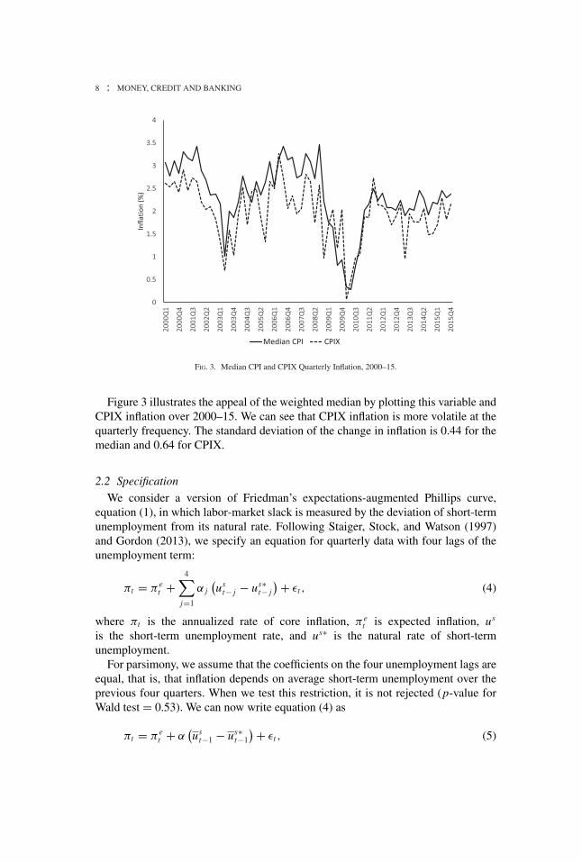
FIG. 4. Short-Term Unemployment and Estimates of Its Natural Rate.

where ust−1 and us∗

t−1 are the averages of us and us∗ from t − 4 through t − 1.In our empirical work, we measure core inflation with weighted median inflation,

as discussed above. We measure the other variables in equation (5) as follows:Expected Inflation: In this section, we do not model the behavior of expectations;

instead, we measure expectations directly with survey data. Specifically, followingpast work such as Fuhrer, Olivei, and Tootell (2009), we measure expected inflationwith the long-term SPF forecasts of CPI inflation shown in Figure 1.3

Short-term Unemployment: As in Figure 2, we define the short-term unemploymentrate as the fraction of the labor force unemployed for 26 weeks or less.

The Natural Rate of Short-term Unemployment: When we estimate Phillips curvesthat include total unemployment, we measure the natural rate u∗ with estimates fromthe Congressional Budget Office (CBO). The CBO does not, however, produce aseries for the natural rate of short-term unemployment, so we must create a proxyfor this variable. We assume this natural rate is proportional to the CBO’s naturalrate for total unemployment: us∗ = gu∗. We estimate the constant g with the ratio ofshort-term to total unemployment at times when total unemployment is close to u∗.This procedure yields g = 0.852.

Figure 4 shows the series for us∗ that we construct. An online Appendix to thispaper describes our procedure for estimating us∗, and the rationale for our approach,in more detail.

3. The SPF forecasts are 10-year predictions of headline inflation, not median inflation. We assume,however, that expected median inflation is the same as expected headline inflation for a 10-year horizon. Inour data, the levels of headline and median inflation over 10-year periods are usually close to each other,and it appears difficult to forecast the difference between the two.


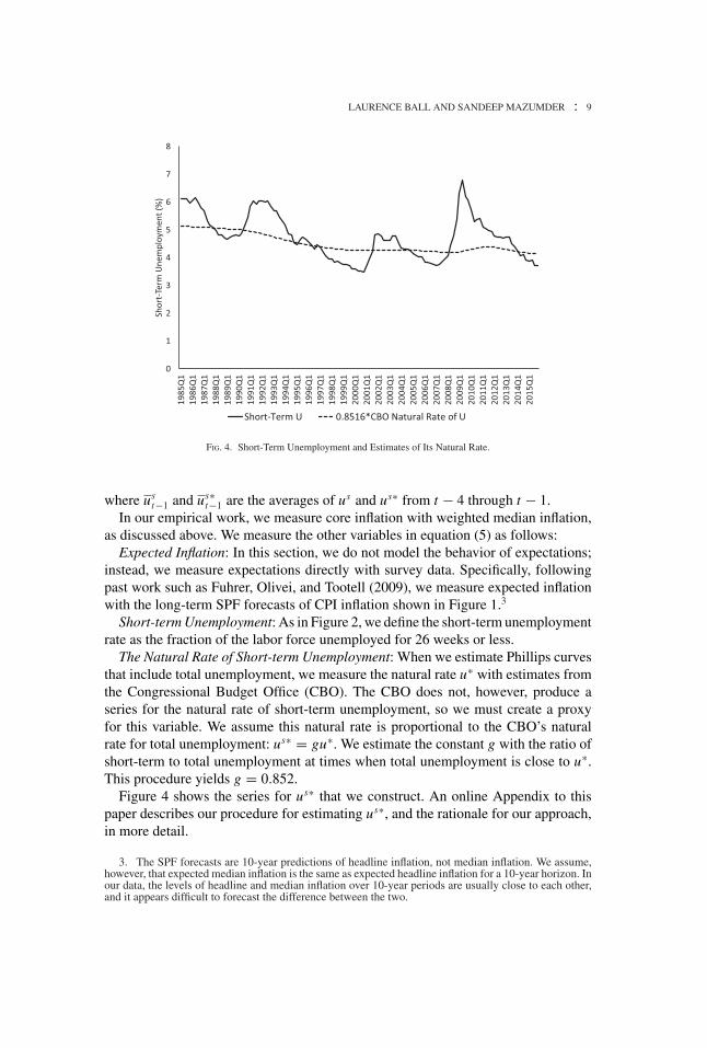
TABLE 1

AN EXPECTATIONS-AUGMENTED PHILLIPS CURVE, 1985–2015

πt = πet + α(us

t−1 − us,∗t−1) + εt

α −0.756(0.077)

DW 1.259SE of Reg. 0.383R

20.824

NOTE: OLS with Newey–West (1987) standard errors in parentheses. πt is median CPI inflation, πet is the average forecast of long-term CPI

inflation from the Survey of Professional Forecasters, ust−1 is the average of the short-term unemployment rate from t − 1 to t − 4, and us∗

t−1is the average of the natural rate of short-term unemployment from t − 1 to t − 4.

2.3 Results

Table 1 presents estimates of the Phillips curve in equation (5) for our 1985–2015sample. The estimated coefficient on short-term unemployment is −0.76, whichmeans that a 1 percentage point rise in average short-term unemployment over theprevious four quarters reduces core inflation by about three quarters of a percentagepoint.4

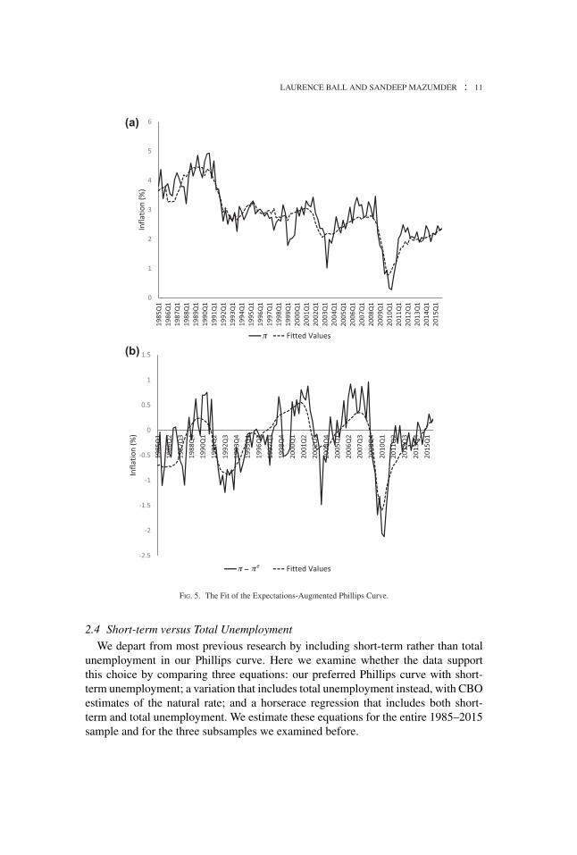
Our Phillips curve explains a large fraction of the variation in core inflation: the

R2

is 0.82. The top panel of Figure 5 illustrates this good fit by plotting the actualand fitted values of core inflation.

This fit partly reflects the fact that actual inflation follows the trend in SPF expectedinflation, which falls from 1985 to the late 1990s and then stabilizes. However, short-term unemployment also explains a substantial part of inflation behavior. To see this

point, we move π et to the left side of (5) and compute the R

2for this version of

the equation. This statistic—the fraction of the variation in πt − π et explained by

short-term unemployment—is 0.61. The bottom panel of Figure 5 plots the actualand fitted values of πt − π e

t .Notice that core inflation falls significantly during three parts of our sample: the

early 1990s, the early 2000s, and 2008–10. These periods align with the last three U.S.recessions, when short-term unemployment was elevated. As a result, our Phillipscurve mostly explains the inflation declines.

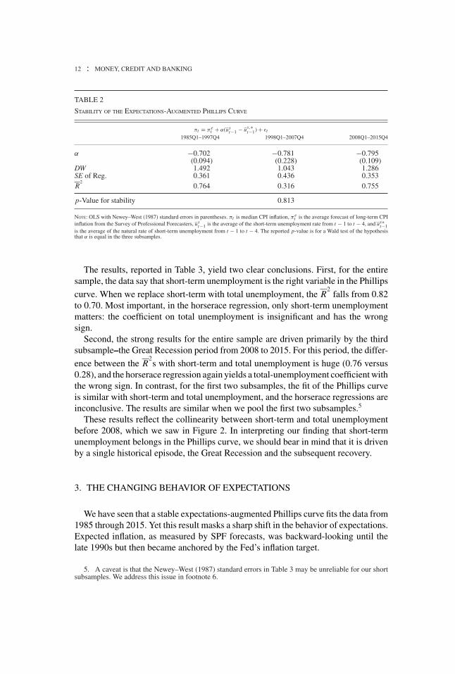
In Table 2, we examine the stability of the Phillips curve by splitting the 1985–2015 sample into three parts. The break dates are 1998, when the reduced-formPhillips curve changed (as shown below); and 2008, the onset of the Great Recession.There is no evidence of instability: the coefficient α is close to the full-sampleestimate of −0.76 in all three subsamples, and a Wald test fails to reject a constant α

(p = 0.81).

4. We have also estimated equation (4), our Phillips curve without the restriction of equal coefficientson the four lags of us − us∗. The estimated coefficients on lags one through four, with standard errors inparentheses, are −0.193 (0.144), −0.219 (0.209), 0.089 (0.275), and −0.444 (0.173). The sum of thesecoefficients is −0.767, which is close to the estimated coefficient on us

t−1 − us∗t−1 in Table 3.


(a)

(b)

− eπ

π

π

FIG. 5. The Fit of the Expectations-Augmented Phillips Curve.

2.4 Short-term versus Total Unemployment

We depart from most previous research by including short-term rather than totalunemployment in our Phillips curve. Here we examine whether the data supportthis choice by comparing three equations: our preferred Phillips curve with short-term unemployment; a variation that includes total unemployment instead, with CBOestimates of the natural rate; and a horserace regression that includes both short-term and total unemployment. We estimate these equations for the entire 1985–2015sample and for the three subsamples we examined before.


TABLE 2

STABILITY OF THE EXPECTATIONS-AUGMENTED PHILLIPS CURVE

πt = πet + α(us

t−1 − us,∗t−1) + εt

1985Q1–1997Q4 1998Q1–2007Q4 2008Q1–2015Q4

α −0.702 −0.781 −0.795(0.094) (0.228) (0.109)

DW 1.492 1.043 1.286SE of Reg. 0.361 0.436 0.353R

20.764 0.316 0.755

p-Value for stability 0.813


inflation from the Survey of Professional Forecasters, ust−1 is the average of the short-term unemployment rate from t − 1 to t − 4, and us∗

t−1is the average of the natural rate of short-term unemployment from t − 1 to t − 4. The reported p-value is for a Wald test of the hypothesisthat α is equal in the three subsamples.

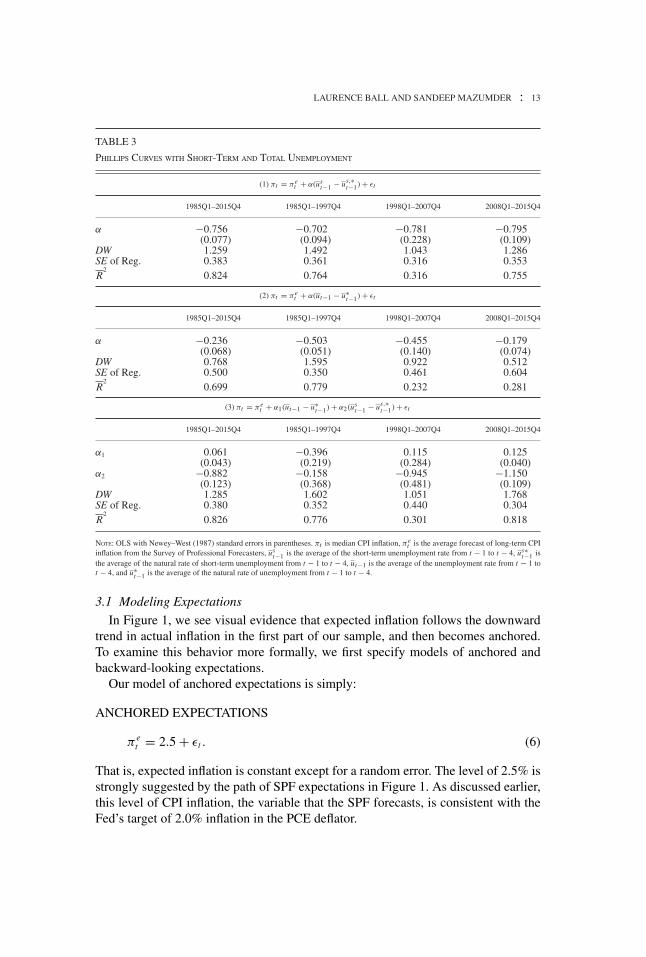
The results, reported in Table 3, yield two clear conclusions. First, for the entiresample, the data say that short-term unemployment is the right variable in the Phillips

curve. When we replace short-term with total unemployment, the R2

falls from 0.82to 0.70. Most important, in the horserace regression, only short-term unemploymentmatters: the coefficient on total unemployment is insignificant and has the wrongsign.

Second, the strong results for the entire sample are driven primarily by the thirdsubsample–the Great Recession period from 2008 to 2015. For this period, the differ-

ence between the R2s with short-term and total unemployment is huge (0.76 versus

0.28), and the horserace regression again yields a total-unemployment coefficient withthe wrong sign. In contrast, for the first two subsamples, the fit of the Phillips curveis similar with short-term and total unemployment, and the horserace regressions areinconclusive. The results are similar when we pool the first two subsamples.5

These results reflect the collinearity between short-term and total unemploymentbefore 2008, which we saw in Figure 2. In interpreting our finding that short-termunemployment belongs in the Phillips curve, we should bear in mind that it is drivenby a single historical episode, the Great Recession and the subsequent recovery.

3. THE CHANGING BEHAVIOR OF EXPECTATIONS

We have seen that a stable expectations-augmented Phillips curve fits the data from1985 through 2015. Yet this result masks a sharp shift in the behavior of expectations.Expected inflation, as measured by SPF forecasts, was backward-looking until thelate 1990s but then became anchored by the Fed’s inflation target.

5. A caveat is that the Newey–West (1987) standard errors in Table 3 may be unreliable for our shortsubsamples. We address this issue in footnote 6.


TABLE 3

PHILLIPS CURVES WITH SHORT-TERM AND TOTAL UNEMPLOYMENT

(1) πt = πet + α(us

t−1 − us,∗t−1) + εt

1985Q1–2015Q4 1985Q1–1997Q4 1998Q1–2007Q4 2008Q1–2015Q4

α −0.756 −0.702 −0.781 −0.795(0.077) (0.094) (0.228) (0.109)

DW 1.259 1.492 1.043 1.286SE of Reg. 0.383 0.361 0.316 0.353R

20.824 0.764 0.316 0.755

(2) πt = πet + α(ut−1 − u∗

t−1) + εt

1985Q1–2015Q4 1985Q1–1997Q4 1998Q1–2007Q4 2008Q1–2015Q4

α −0.236 −0.503 −0.455 −0.179(0.068) (0.051) (0.140) (0.074)

DW 0.768 1.595 0.922 0.512SE of Reg. 0.500 0.350 0.461 0.604R

20.699 0.779 0.232 0.281

(3) πt = πet + α1(ut−1 − u∗

t−1) + α2(ust−1 − us,∗

t−1) + εt

1985Q1–2015Q4 1985Q1–1997Q4 1998Q1–2007Q4 2008Q1–2015Q4

α1 0.061 −0.396 0.115 0.125(0.043) (0.219) (0.284) (0.040)

α2 −0.882 −0.158 −0.945 −1.150(0.123) (0.368) (0.481) (0.109)

DW 1.285 1.602 1.051 1.768SE of Reg. 0.380 0.352 0.440 0.304R

20.826 0.776 0.301 0.818


inflation from the Survey of Professional Forecasters, ust−1 is the average of the short-term unemployment rate from t − 1 to t − 4, us∗

t−1 isthe average of the natural rate of short-term unemployment from t − 1 to t − 4, ut−1 is the average of the unemployment rate from t − 1 tot − 4, and u∗

t−1 is the average of the natural rate of unemployment from t − 1 to t − 4.

3.1 Modeling Expectations

In Figure 1, we see visual evidence that expected inflation follows the downwardtrend in actual inflation in the first part of our sample, and then becomes anchored.To examine this behavior more formally, we first specify models of anchored andbackward-looking expectations.

Our model of anchored expectations is simply:

ANCHORED EXPECTATIONS

π et = 2.5 + εt . (6)

That is, expected inflation is constant except for a random error. The level of 2.5% isstrongly suggested by the path of SPF expectations in Figure 1. As discussed earlier,this level of CPI inflation, the variable that the SPF forecasts, is consistent with theFed’s target of 2.0% inflation in the PCE deflator.


In our backward-looking model, we assume that expected inflation depends onpast levels of core inflation. Following Gordon (2013), we include a large number oflags, which allows expectations to adjust slowly to changes in actual inflation. Wemake the accelerationist assumption that the coefficients on the lags sum to one.

For parsimony, we also assume that the coefficients decline exponentially as the laglength rises. This assumption yields a single parameter to be estimated, and we findthat it fits the data well. In principle, the exponential specification includes infinitelags, but we truncate them at 40 quarters. Our equation is

BACKWARD-LOOKING EXPECTATIONS

π et = 1

1 − γ 40

[(1 − γ )πt−1 + γ (1 − γ )πt−2 + . . . + γ 39(1 − γ )πt−40

] + εt , (7)

where γ determines the rate of decay of the lag coefficients. (The term outside thebrackets makes the coefficients sum to one.)

We hypothesize that expectations shifted from backward-looking to anchored dur-ing our sample period. To test this idea, we examine a specification that nests the twomodels:

π et = λ2.5 + (1 − λ)

1

1 − γ 40

[(1 − γ )πt−1 + γ (1 − γ )πt−2 + · · ·

+ γ 39(1 − γ )πt−40] + εt . (8)

Here, expected inflation from the SPF is a weighted average of two terms, the 2.5%anchor and our backward-looking specification. We ask whether the coefficients λ

and 1 − λ have changed over time.Specifically, we test for a change in λ at an unknown break date using the Andrews

(1993) sup-Wald test. We then examine estimates of equation (8) before and afterthe date that yields the highest Wald statistic. In this exercise, we assume that theparameter γ in the backward-looking model is constant over time.

3.2 Results

The Andrews test rejects stability of λ and 1 − λ, the weights on backward-lookingand anchored expectations. The sup-Wald statistic is 68.3, which greatly exceeds the1% critical value of 12.4 (for 15% trimming of the data).

The break date that produces the highest Wald statistic is 1998Q1. The first columnof Table 4 presents estimates of equation (8) with that break, and reveals a largechange in λ. For 1985–97, the estimated λ is 0.07, and it is statistically insignificant;for 1998–2015, the estimate is 0.77. These results mean that expectations werebackward-looking before 1998, but then became strongly (although not completely)anchored.

The second column of Table 4 presents estimates of (8) with the restrictions thatλ = 0 before 1998Q1 and λ = 1 after 1998Q1, meaning that expectations shift from


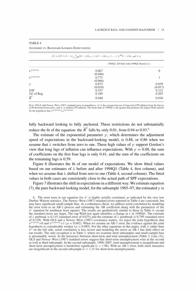
TABLE 4

ANCHORED VS. BACKWARD-LOOKING EXPECTATIONS

πet = λ2.5 + (1 − λ) 1

1−γ 40 [(1 − γ )πt−1 + γ (1 − γ )πt−2 + . . . + γ 39(1 − γ )πt−40] + εt

1985Q1–2015Q4 (with 1998Q1 Break in λ)

λprebreak 0.067 0(0.046)

λpostbreak 0.773 1(0.066)

γ 0.875 0.859(0.018) (0.017)

DW 0.357 0.312SE of Reg. 0.189 0.203R

20.940 0.930

NOTE: NLLS with Newey–West (1987) standard errors in parentheses. πet is the average forecast of long-term CPI inflation from the Survey

of Professional Forecasters, and πt is median CPI inflation. The break date of 1998Q1 is the quarter that produces the largest Wald statisticfor the hypothesis that λprebreak=λpostbreak .

fully backward looking to fully anchored. These restrictions do not substantially

reduce the fit of the equation: the R2

falls by only 0.01, from 0.94 to 0.93.6

The estimate of the exponential parameter γ , which determines the adjustmentspeed of expectations in the backward-looking model, is 0.88, or 0.86 when weassume that λ switches from zero to one. These high values of γ support Gordon’sview that long lags of inflation can influence expectations. With γ = 0.88, the sumof coefficients on the first four lags is only 0.41, and the sum of the coefficients onthe remaining lags is 0.59.

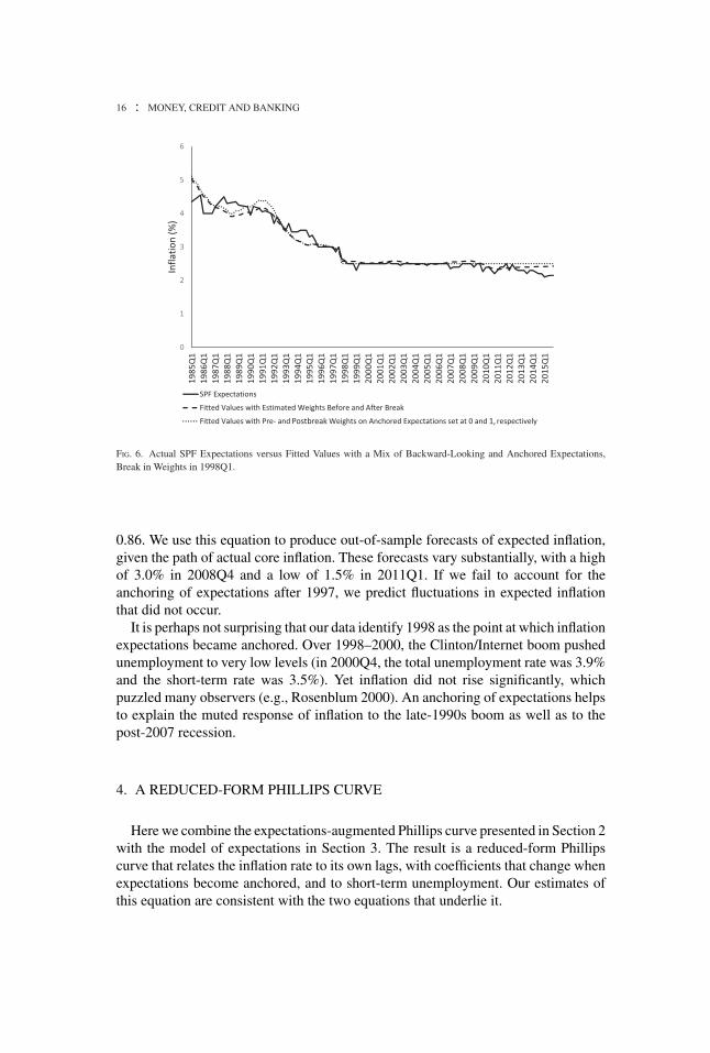
Figure 6 illustrates the fit of our model of expectations. We show fitted valuesbased on our estimates of λ before and after 1998Q1 (Table 4, first column), andwhen we assume that λ shifted from zero to one (Table 4, second column). The fittedvalues in both cases are consistently close to the actual path of SPF expectations.

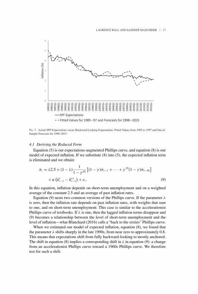
Figure 7 illustrates the shift in expectations in a different way. We estimate equation(7), the pure backward-looking model, for the subsample 1985–97; the estimated γ is

6. The error term in our equation for π e is highly serially correlated, as indicated by the very lowDurbin–Watson statistics. The Newey–West (1987) standard errors reported in Table 4 are consistent, butmay have significant small-sample bias. As a robustness check, we address serial correlation by modelingthe error term as an AR-1 process and estimating the AR coefficient along with the parameters of theπ e equation by nonlinear least squares. The results are qualitatively similar to those in Table 4, exceptthe standard errors are larger. The sup-Wald test again identifies a change in λ in 1998Q1. The estimateof λ prebreak is 0.115 (standard error of 0.075) and the estimate of λ postbreak is 0.799 (standard errorof 0.129). With OLS and a Newey–West (1987) covariance matrix, we reject the joint hypothesis thatλprebreak=0 and λpostbreak=1 (p = 0.002). When we assume an AR-1 error, the evidence against the jointhypothesis is considerably weaker (p = 0.095). For the other equations in this paper, with π rather thanπ e on the left side, serial correlation is less severe and modeling the errors as AR-1 has little effect onour results. The only exception is in Table 3, where we examine short subsamples and small-sample biasis presumably worse. In the horserace between short-term and total unemployment (Table 3, Line (3)),OLS and Newey–West (1987) standard errors suggest that short-term unemployment wins in the secondas well as third subsample. In the second subsample, 1998–2007, total unemployment is insignificant andshort-term unemployment is borderline significant (t = 1.96). With an AR-1 error, both slack measuresare insignificant in the second subsample (t = 1.31 for short-term unemployment).


Postbreak 1,

FIG. 6. Actual SPF Expectations versus Fitted Values with a Mix of Backward-Looking and Anchored Expectations,Break in Weights in 1998Q1.

0.86. We use this equation to produce out-of-sample forecasts of expected inflation,given the path of actual core inflation. These forecasts vary substantially, with a highof 3.0% in 2008Q4 and a low of 1.5% in 2011Q1. If we fail to account for theanchoring of expectations after 1997, we predict fluctuations in expected inflationthat did not occur.

It is perhaps not surprising that our data identify 1998 as the point at which inflationexpectations became anchored. Over 1998–2000, the Clinton/Internet boom pushedunemployment to very low levels (in 2000Q4, the total unemployment rate was 3.9%and the short-term rate was 3.5%). Yet inflation did not rise significantly, whichpuzzled many observers (e.g., Rosenblum 2000). An anchoring of expectations helpsto explain the muted response of inflation to the late-1990s boom as well as to thepost-2007 recession.

4. A REDUCED-FORM PHILLIPS CURVE

Here we combine the expectations-augmented Phillips curve presented in Section 2with the model of expectations in Section 3. The result is a reduced-form Phillipscurve that relates the inflation rate to its own lags, with coefficients that change whenexpectations become anchored, and to short-term unemployment. Our estimates ofthis equation are consistent with the two equations that underlie it.


1985—97 1998—2015

FIG. 7. Actual SPF Expectations versus Backward-Looking Expectations: Fitted Values from 1985 to 1997 and Out-of-Sample Forecasts for 1998–2015.

4.1 Deriving the Reduced Form

Equation (5) is our expectations-augmented Phillips curve, and equation (8) is ourmodel of expected inflation. If we substitute (8) into (5), the expected inflation termis eliminated and we obtain:

πt = λ2.5 + (1 − λ)1

1 − γ 40

[(1 − γ )πt−1 + · · · + γ 39(1 − γ )πt−40

]

+α(us

t−1 − us∗t−1

) + εt . (9)

In this equation, inflation depends on short-term unemployment and on a weightedaverage of the constant 2.5 and an average of past inflation rates.

Equation (9) nests two common versions of the Phillips curve. If the parameter λ

is zero, then the inflation rate depends on past inflation rates, with weights that sumto one, and on short-term unemployment. This case is similar to the accelerationistPhillips curve of textbooks. If λ is one, then the lagged inflation terms disappear and(9) becomes a relationship between the level of short-term unemployment and thelevel of inflation—what Blanchard (2016) calls a “back to the sixties” Phillips curve.

When we estimated our model of expected inflation, equation (8), we found thatthe parameter λ shifts sharply in the late 1990s, from near zero to approximately 0.8.This means that expectations shift from fully backward-looking to mostly anchored.The shift in equation (8) implies a corresponding shift in λ in equation (9): a changefrom an accelerationist Phillips curve toward a 1960s Phillips curve. We thereforetest for such a shift.


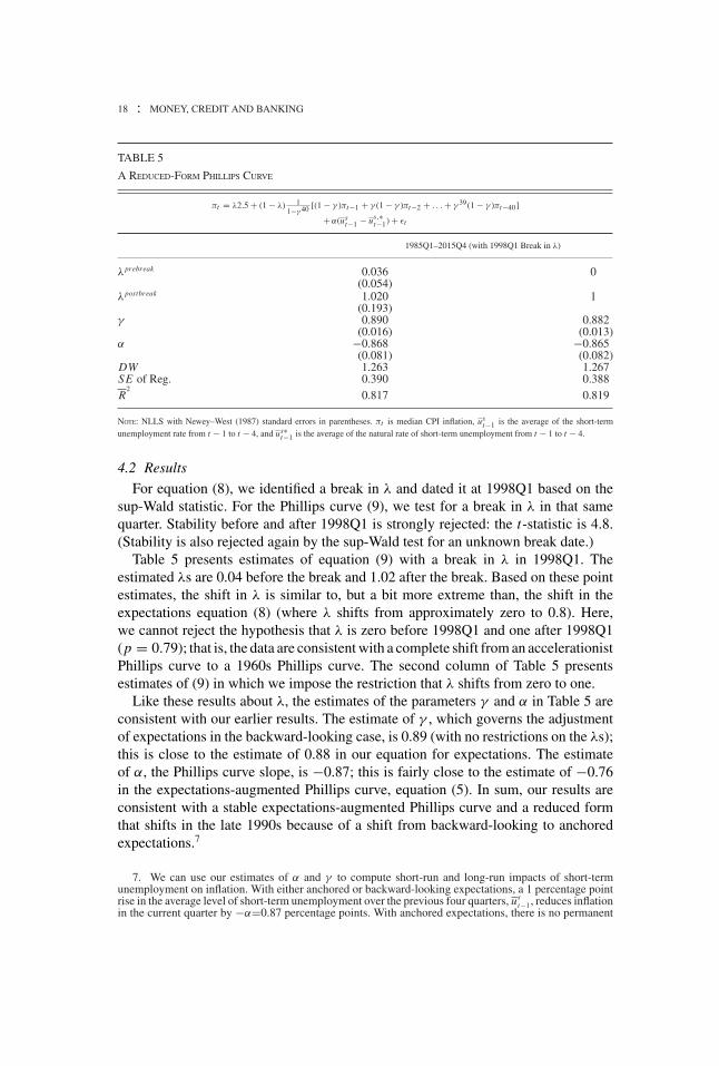
TABLE 5

A REDUCED-FORM PHILLIPS CURVE

πt = λ2.5 + (1 − λ) 11−γ 40 [(1 − γ )πt−1 + γ (1 − γ )πt−2 + . . . + γ 39(1 − γ )πt−40]

+ α(ust−1 − us,∗

t−1) + εt


λprebreak 0.036 0(0.054)

λpostbreak 1.020 1(0.193)

γ 0.890 0.882(0.016) (0.013)

α −0.868 −0.865(0.081) (0.082)

DW 1.263 1.267SE of Reg. 0.390 0.388R

20.817 0.819

NOTE: NLLS with Newey–West (1987) standard errors in parentheses. πt is median CPI inflation, ust−1 is the average of the short-term

unemployment rate from t − 1 to t − 4, and us∗t−1 is the average of the natural rate of short-term unemployment from t − 1 to t − 4.

4.2 Results

For equation (8), we identified a break in λ and dated it at 1998Q1 based on thesup-Wald statistic. For the Phillips curve (9), we test for a break in λ in that samequarter. Stability before and after 1998Q1 is strongly rejected: the t-statistic is 4.8.(Stability is also rejected again by the sup-Wald test for an unknown break date.)

Table 5 presents estimates of equation (9) with a break in λ in 1998Q1. Theestimated λs are 0.04 before the break and 1.02 after the break. Based on these pointestimates, the shift in λ is similar to, but a bit more extreme than, the shift in theexpectations equation (8) (where λ shifts from approximately zero to 0.8). Here,we cannot reject the hypothesis that λ is zero before 1998Q1 and one after 1998Q1(p = 0.79); that is, the data are consistent with a complete shift from an accelerationistPhillips curve to a 1960s Phillips curve. The second column of Table 5 presentsestimates of (9) in which we impose the restriction that λ shifts from zero to one.

Like these results about λ, the estimates of the parameters γ and α in Table 5 areconsistent with our earlier results. The estimate of γ , which governs the adjustmentof expectations in the backward-looking case, is 0.89 (with no restrictions on the λs);this is close to the estimate of 0.88 in our equation for expectations. The estimateof α, the Phillips curve slope, is −0.87; this is fairly close to the estimate of −0.76in the expectations-augmented Phillips curve, equation (5). In sum, our results areconsistent with a stable expectations-augmented Phillips curve and a reduced formthat shifts in the late 1990s because of a shift from backward-looking to anchoredexpectations.7

7. We can use our estimates of α and γ to compute short-run and long-run impacts of short-termunemployment on inflation. With either anchored or backward-looking expectations, a 1 percentage pointrise in the average level of short-term unemployment over the previous four quarters, us

t−1, reduces inflationin the current quarter by −α=0.87 percentage points. With anchored expectations, there is no permanent


Postbreak 1,

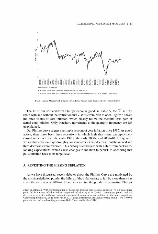
FIG. 8. Actual Median CPI Inflation versus Fitted Values from Reduced-Form Phillips Curve.

The fit of our reduced-form Phillips curve is good: in Table 5, the R2

is 0.82(both with and without the restriction that λ shifts from zero to one). Figure 8 showsthe fitted values of core inflation, which closely follow the medium-term path ofactual core inflation. Only transitory movements at the quarterly frequency are leftunexplained.

Our Phillips curve suggests a simple account of core inflation since 1985. As notedabove, there have been three recessions in which high short-term unemploymentcaused inflation to fall: the early 1990s, the early 2000s, and 2008–10. In Figure 8,we see that inflation stayed roughly constant after its first decrease, but the second andthird decreases were reversed. This history is consistent with a shift from backward-looking expectations, which cause changes in inflation to persist, to anchoring thatpulls inflation back to its target level.

5. REVISITING THE MISSING DEFLATION

As we have discussed, recent debates about the Phillips Curve are motivated bythe missing-deflation puzzle: the failure of the inflation rate to fall by more than it hassince the recession of 2008–9. Here, we examine the puzzle by estimating Phillips

effect on inflation. With our formulation of backward-looking expectations, equation (7), a 1 percentagepoint fall in current inflation reduces expected inflation by (1 − γ )=0.11 percentage points, and thedecrease in expected inflation causes a permanent decrease in actual inflation of the same magnitude.Combining these facts, a one-point rise in us

t−1 causes a permanent inflation decrease of α(1 − γ ) = 0.095points in the backward-looking case (see Ball, Chari, and Mishra 2016).


curves with pre-2008 data and then forecasting inflation over 2008–15. We see thata conventional Phillips curve predicts a deflation that did not occur, and that thisanomaly is resolved with the specification proposed in this paper.

For this exercise, we estimate Phillips curves over the period 1985–97. We assumebackward-looking inflation expectations, equation (7), because that assumption fitsthe data for 1985–97. We consider both short-term and total unemployment as mea-sures of economic slack. We saw that those variables were highly collinear before1998, so we expect the fit of the Phillips curve to be similar in the two cases. Ourspecifications are

πt = 1

1 − γ 40

[(1 − γ )πt−1 + . . . + γ 39(1 − γ )πt−40

]

+α(us

t−1 − us∗t−1

) + εt (10)

and

πt = 1

1 − γ 40

[(1 − γ )πt−1 + . . . + γ 39(1 − γ )πt−40

]

+α(ut−1 − u∗

t−1

) + εt , (11)

where us is short-term unemployment and u is total unemployment. Note that equation(10) is a special case of our reduced-form Phillips curve, equation (9), with noanchoring of expectations (λ = 0).

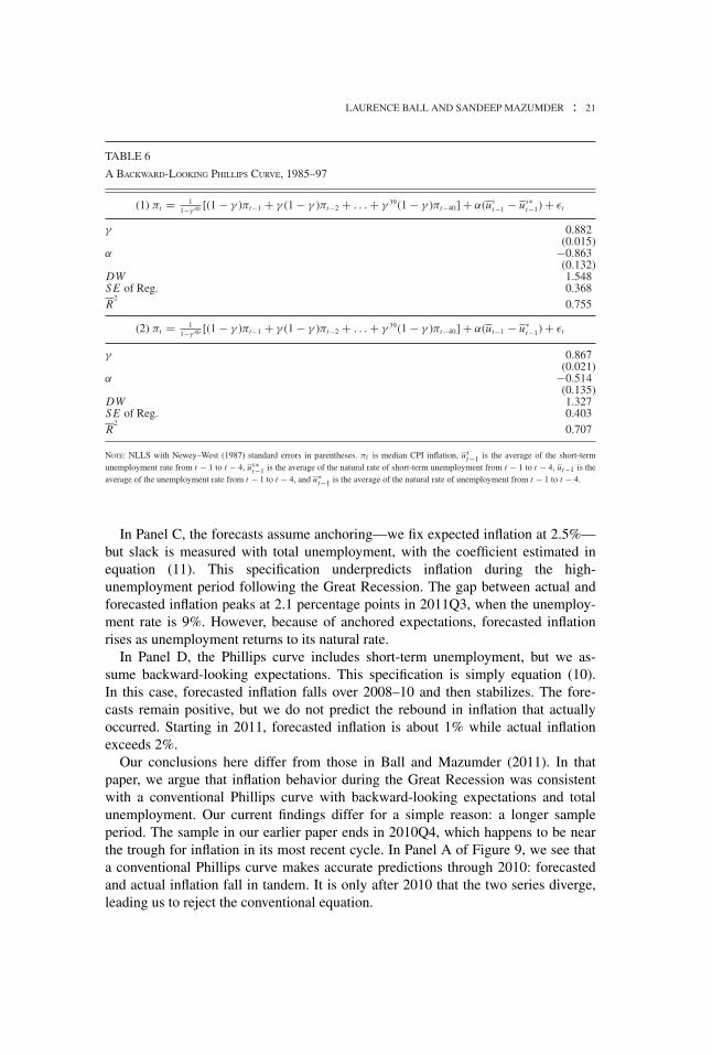
Table 6 presents our estimates of (10) and (11). The fit is good (R2>0.7) with either

short-term or total unemployment in the equation. The estimates of the parameter γ

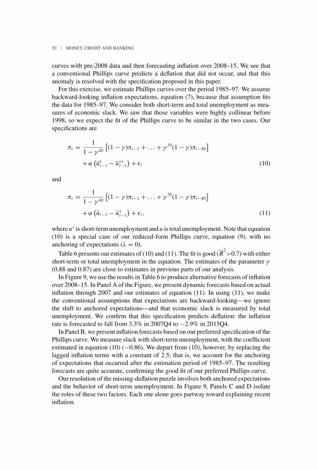
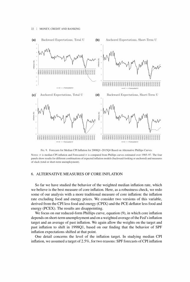
(0.88 and 0.87) are close to estimates in previous parts of our analysis.In Figure 9, we use the results in Table 6 to produce alternative forecasts of inflation

over 2008–15. In Panel A of the Figure, we present dynamic forecasts based on actualinflation through 2007 and our estimates of equation (11). In using (11), we makethe conventional assumptions that expectations are backward-looking—we ignorethe shift to anchored expectations—and that economic slack is measured by totalunemployment. We confirm that this specification predicts deflation: the inflationrate is forecasted to fall from 3.3% in 2007Q4 to −2.9% in 2015Q4.

In Panel B, we present inflation forecasts based on our preferred specification of thePhillips curve. We measure slack with short-term unemployment, with the coefficientestimated in equation (10) (−0.86). We depart from (10), however, by replacing thelagged inflation terms with a constant of 2.5; that is, we account for the anchoringof expectations that occurred after the estimation period of 1985–97. The resultingforecasts are quite accurate, confirming the good fit of our preferred Phillips curve.

Our resolution of the missing-deflation puzzle involves both anchored expectationsand the behavior of short-term unemployment. In Figure 9, Panels C and D isolatethe roles of these two factors. Each one alone goes partway toward explaining recentinflation.


TABLE 6

A BACKWARD-LOOKING PHILLIPS CURVE, 1985–97

(1) πt = 11−γ 40 [(1 − γ )πt−1 + γ (1 − γ )πt−2 + . . . + γ 39(1 − γ )πt−40] + α(us

t−1 − us∗t−1) + εt

γ 0.882(0.015)

α −0.863(0.132)


20.755

(2) πt = 11−γ 40 [(1 − γ )πt−1 + γ (1 − γ )πt−2 + . . . + γ 39(1 − γ )πt−40] + α(ut−1 − u∗

t−1) + εt

γ 0.867(0.021)

α −0.514(0.135)


20.707

NOTE: NLLS with Newey–West (1987) standard errors in parentheses. πt is median CPI inflation, ust−1 is the average of the short-term

unemployment rate from t − 1 to t − 4, us∗t−1 is the average of the natural rate of short-term unemployment from t − 1 to t − 4, ut−1 is the

average of the unemployment rate from t − 1 to t − 4, and u∗t−1 is the average of the natural rate of unemployment from t − 1 to t − 4.

In Panel C, the forecasts assume anchoring—we fix expected inflation at 2.5%—but slack is measured with total unemployment, with the coefficient estimated inequation (11). This specification underpredicts inflation during the high-unemployment period following the Great Recession. The gap between actual andforecasted inflation peaks at 2.1 percentage points in 2011Q3, when the unemploy-ment rate is 9%. However, because of anchored expectations, forecasted inflationrises as unemployment returns to its natural rate.

In Panel D, the Phillips curve includes short-term unemployment, but we as-sume backward-looking expectations. This specification is simply equation (10).In this case, forecasted inflation falls over 2008–10 and then stabilizes. The fore-casts remain positive, but we do not predict the rebound in inflation that actuallyoccurred. Starting in 2011, forecasted inflation is about 1% while actual inflationexceeds 2%.

Our conclusions here differ from those in Ball and Mazumder (2011). In thatpaper, we argue that inflation behavior during the Great Recession was consistentwith a conventional Phillips curve with backward-looking expectations and totalunemployment. Our current findings differ for a simple reason: a longer sampleperiod. The sample in our earlier paper ends in 2010Q4, which happens to be nearthe trough for inflation in its most recent cycle. In Panel A of Figure 9, we see thata conventional Phillips curve makes accurate predictions through 2010: forecastedand actual inflation fall in tandem. It is only after 2010 that the two series diverge,leading us to reject the conventional equation.


(a) (b)

(c) (d)

Backward Expectations, Total U Anchored Expectations, Short-Term U

Anchored Expectations, Total U Backward Expectations, Short-Term U

π π π π

π ππ π

FIG. 9. Forecasts for Median CPI Inflation for 2008Q1–2015Q4 Based on Alternative Phillips Curves.

NOTES: π is median CPI inflation and Forecasted π is computed from Phillips curves estimated over 1985–97. The fourpanels show results for different combinations of expected inflation models (backward-looking or anchored) and measuresof slack (total or short-term unemployment).

6. ALTERNATIVE MEASURES OF CORE INFLATION

So far we have studied the behavior of the weighted median inflation rate, whichwe believe is the best measure of core inflation. Here, as a robustness check, we redosome of our analysis with a more traditional measure of core inflation: the inflationrate excluding food and energy prices. We consider two versions of this variable,derived from the CPI less food and energy (CPIX) and the PCE deflator less food andenergy (PCEX). The results are disappointing.

We focus on our reduced-form Phillips curve, equation (9), in which core inflationdepends on short-term unemployment and on a weighted average of the Fed’s inflationtarget and an average of past inflation. We again allow the weights on the target andpast inflation to shift in 1998Q1, based on our finding that the behavior of SPFinflation expectations shifted at that point.

One detail concerns the level of the inflation target. In studying median CPIinflation, we assumed a target of 2.5%, for two reasons: SPF forecasts of CPI inflation


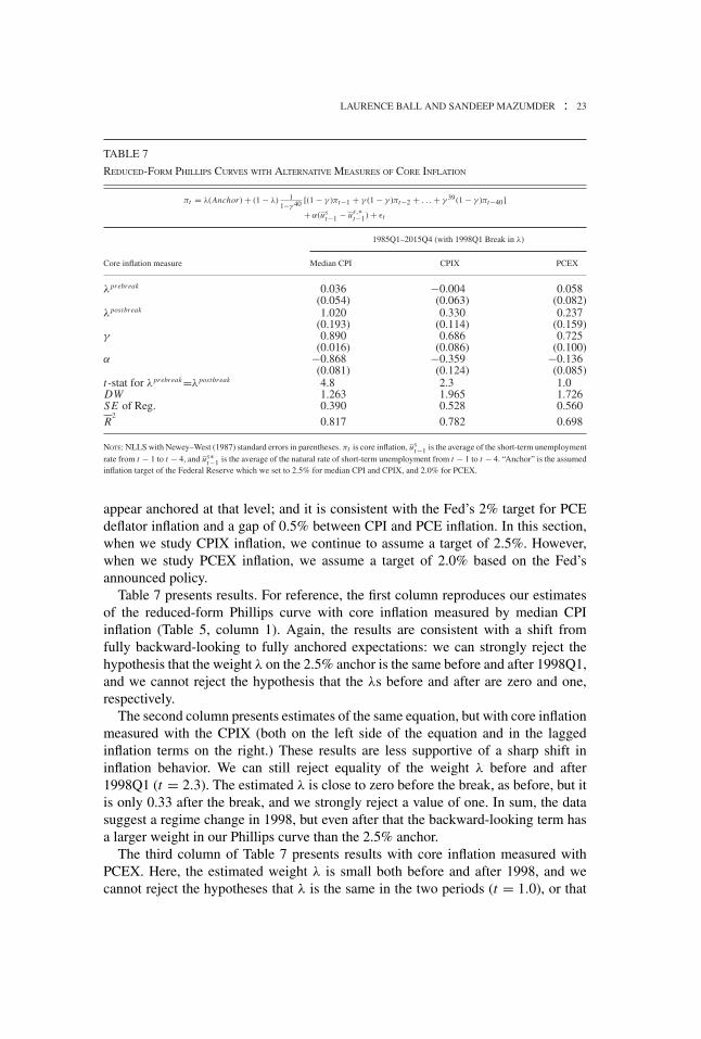
TABLE 7

REDUCED-FORM PHILLIPS CURVES WITH ALTERNATIVE MEASURES OF CORE INFLATION

πt = λ(Anchor ) + (1 − λ) 11−γ 40 [(1 − γ )πt−1 + γ (1 − γ )πt−2 + . . . + γ 39(1 − γ )πt−40]

+ α(ust−1 − us,∗

t−1) + εt


Core inflation measure Median CPI CPIX PCEX

λprebreak 0.036 −0.004 0.058(0.054) (0.063) (0.082)

λpostbreak 1.020 0.330 0.237(0.193) (0.114) (0.159)

γ 0.890 0.686 0.725(0.016) (0.086) (0.100)

α −0.868 −0.359 −0.136(0.081) (0.124) (0.085)

t-stat for λprebreak=λpostbreak 4.8 2.3 1.0DW 1.263 1.965 1.726SE of Reg. 0.390 0.528 0.560R

20.817 0.782 0.698

NOTE: NLLS with Newey–West (1987) standard errors in parentheses. πt is core inflation, ust−1 is the average of the short-term unemployment

rate from t − 1 to t − 4, and us∗t−1 is the average of the natural rate of short-term unemployment from t − 1 to t − 4. “Anchor” is the assumed

inflation target of the Federal Reserve which we set to 2.5% for median CPI and CPIX, and 2.0% for PCEX.

appear anchored at that level; and it is consistent with the Fed’s 2% target for PCEdeflator inflation and a gap of 0.5% between CPI and PCE inflation. In this section,when we study CPIX inflation, we continue to assume a target of 2.5%. However,when we study PCEX inflation, we assume a target of 2.0% based on the Fed’sannounced policy.

Table 7 presents results. For reference, the first column reproduces our estimatesof the reduced-form Phillips curve with core inflation measured by median CPIinflation (Table 5, column 1). Again, the results are consistent with a shift fromfully backward-looking to fully anchored expectations: we can strongly reject thehypothesis that the weight λ on the 2.5% anchor is the same before and after 1998Q1,and we cannot reject the hypothesis that the λs before and after are zero and one,respectively.

The second column presents estimates of the same equation, but with core inflationmeasured with the CPIX (both on the left side of the equation and in the laggedinflation terms on the right.) These results are less supportive of a sharp shift ininflation behavior. We can still reject equality of the weight λ before and after1998Q1 (t = 2.3). The estimated λ is close to zero before the break, as before, but itis only 0.33 after the break, and we strongly reject a value of one. In sum, the datasuggest a regime change in 1998, but even after that the backward-looking term hasa larger weight in our Phillips curve than the 2.5% anchor.

The third column of Table 7 presents results with core inflation measured withPCEX. Here, the estimated weight λ is small both before and after 1998, and wecannot reject the hypotheses that λ is the same in the two periods (t = 1.0), or that


it is zero in both periods (p-value = 0.17). Thus the data are consistent with fullybackward-looking expectations for the entire period from 1985 to 2015. Notice alsothat the coefficient on short-term unemployment is small, with borderline significance(t = 1.6): we lack strong evidence of an unemployment-inflation trade-off.

Our research has focused on the behavior of median CPI inflation because it is ourpreferred measure of core inflation. At this point, we have a poor understanding ofthe behavior of CPIX and PCEX inflation. The difficulty of explaining these variablesmay reflect their volatility at the quarterly frequency, illustrated above in Figure 3.For our sample period of 1985–2015, the standard deviation of the quarterly changein inflation is 0.65 percentage points for CPIX and 0.69 for PCEX, compared to 0.44for median inflation.

7. CONCLUSION

One of Mankiw’s (2014) 10 principles of economics is, “Society faces a short-runtrade-off between inflation and unemployment.” This trade-off, the Phillips curve,is critically important for monetary policy and for forecasting inflation. It would beextraordinarily useful to discover a specification of the Phillips curve that fits the datareliably.

Unfortunately, researchers have repeatedly needed to modify the Phillips curve tofit new data. Friedman added expected inflation to the specification in Samuelsonand Solow (1960). Subsequent authors have added supply shocks (Gordon 1982),time variation in the Phillips-curve slope (Ball, Mankiw, and Romer 1988), and timevariation in the natural rate of unemployment (Staiger, Stock, and Watson 1997). Eachmodification helped explain past data, but, as Stock and Watson (2010) observe, thehistory of the Phillips curve “is one of apparently stable relationships falling apartupon publication.” Ball and Mazumder (2011) is a poignant example.

Nonetheless, because of the practical importance of the Phillips curve, researchersmust continue to search for better specifications. This paper proposes a simple Phillipscurve that fits the recent behavior of core inflation, at least when core inflationis measured by median inflation. Our key assumptions are that labor-market slackis measured by short-term unemployment, and that expected inflation has becomeanchored at a constant level.

Our two key assumptions have been proposed by a number of researchers, butothers have questioned them. For example, Abraham (2014) reports that the jobfinding rates of the short-term and long-term unemployed do not differ dramatically,making it unclear why only short-term unemployment affects inflation. The apparentanchoring of inflation expectations also lacks a full explanation. The data suggest asharp regime shift in the late 1990s, but it is not obvious why the Fed’s inflation targetbecame credible during that period.

Nonetheless, we believe that the Phillips curve proposed in this paper providesa plausible account of inflation behavior since 1985. Going forward, new data will


help us determine the robustness of our conclusions. One risk is that expectationswill become unmoored because the Fed changes its inflation target, or actual inflationdeviates greatly from the target. If that happens, future Phillips curves will need toincorporate the new behavior of expectations.

While our Phillips-curve specification draws on recent research, we have ignoredone idea that is prominent in recent work on inflation: downward nominal wage rigid-ity. We neglect downward rigidity primarily because our Phillips curve fits the datawithout it. Research will surely continue on the roles of short-term unemployment,anchored expectations, and downward wage rigidity in explaining recent inflationbehavior.8

LITERATURE CITED

Abraham, Katharine. (2014) “Discussion of Krueger, Cramer, and Cho, ‘Are the Long-TermUnemployed on the Margins of the Labor Market?’” Brookings Papers on Economic Activity,45, 281–87.

Andrews, Donald. (1993) “Tests for Parameter Instability and Structural Change with UnknownChange Point.” Econometrica, 61, 821–56.

Ball, Laurence, Anuscha Chari, and Prachi Mishra. (2016) “Understanding Inflation in India.”NBER Working Paper 22948.

Ball, Laurence, N. Gregory Mankiw, and David Romer. (1988) “The New Keynsesian Eco-nomics and the Output-Inflation Trade-Off.” Brookings Papers on Economic Activity, 19,1–82.

Ball, Laurence and Sandeep Mazumder. (2011) “Inflation Dynamics and the Great Recession.”Brookings Papers on Economic Activity, 42, 337–405.

Bernanke, Ben S. (2010) “The Economic Outlook and Monetary Policy.” Speech at the FederalReserve Bank of Kansas City Economic Symposium, Jackson Hole, Wyoming.

Blanchard, Oliver. (2016) “The Phillips Curve: Back to the ’60s?” American Economic Review,106, 31–4.

Coibion, Oliver, and Yuriy Gorodnichenko. (2015) “Is the Phillips Curve Alive and Well afterAll? Inflation Expectations and the Missing Disinflation.” American Economic Journal:Macroeconomics, 7, 197–232.

Daly, Mary, and Bart Hobijn. (2014) “Downward Nominal Wage Rigidities Bend the PhillipsCurve.” Journal of Money, Credit and Banking, 46, 51–93.

Dickens, William. (2010) “Has the Recession Increased the NAIRU?” Mimeo, BrookingsInstitution.

Friedman, Milton. (1968) “The Role of Monetary Policy.” American Economic Review, 58,1–17.

Fuhrer, Jeffrey, Giovanni Olivei, and Geoffrey Tootell. (2009) “Empirical Estimates of Chang-ing Inflation Dynamics.” Working Papers 09–4, Federal Reserve Bank of Boston.

8. Recent analyses of downward wage rigidity include Dickens (2010), Schmitt-Grohe and Uribe(2017), Daly and Hobijn (2014), and numerous blog posts by Paul Krugman. Recent research on inflationhas also explored the roles of oil prices and consumer expectations (Coibion and Gorodnichenko 2015);weak balance sheets of firms (Gilchrist et al. 2017); and uncertainty about regional economic conditions(Murphy 2014).


Galı́, Jordi. (2008). Monetary Policy, Inflation, and the Business Cycle: An Introduction to theNew Keynesian Framework. Princeton, NJ: Princeton University Press.

Gilchrist, Simon, Raphael Schoenle, Jae Sim, and Egon Zakrajsek. (2017) “Inflation Dynamicsduring the Financial Crisis.” American Economic Review, 107, 785–823.

Gordon, Robert. (1982) “Inflation, Flexible Exchange Rates, and the Natural Rate of Unem-ployment.” In Workers, Jobs, and Inflation, edited by M. Baily, pp. 89–158. Washington,DC: The Brookings Institution.

Gordon, Robert. (2013) “The Phillips Curve is Alive and Well: Inflation and the NAIRU duringthe Slow Recovery.” Working Paper 19390, National Bureau of Economic Research.

IMF. (2013) “The Dog That Didn’t Bark: Has Inflation Been Muzzled or Was It Just Sleeping?”World Economic Outlook, International Monetary Fund.

Krueger, Alan, Judd Cramer, and David Cho. (2014) “Are the Long-Term Unemployed on theMargins of the Labor Market?” Brookings Papers on Economic Activity, 45, 229–80.

Krugman, Paul. (2014) “Inflation, Unemployment, Ignorance.” New York Times Blog.

Llaudes, Ricardo. (2005) “The Phillips Curve and Long-Term Unemployment.” Working PaperSeries 441, European Central Bank.

Mankiw, N. Gregory. (2014) Principles of Economics, 7th ed. Victoria, Australia: CengageLearning.

Mishkin, Frederic. (2007) “Inflation Dynamics.” International Finance, 10, 317–34.

Murphy, Robert. (2014) “Explaining Inflation in the Aftermath of the Great Recession.”Journal of Macroeconomics, 40, 228–44.

Newey, Whitney, and Kenneth West. (1987) “A Simple, Positive Semi-Definite, Heteroskedas-ticity and Autocorrelation Consistent Covariance Matrix.” Econometrica, 55, 703–08.

Nickell, Stephen. (1987) “Why is Wage Inflation in Britain So High?” Oxford Bulletin ofEconomics and Statistics, 49, 103–28.

Phillips, Alban William. (1958) “The Relation between Unemployment and the Rate of Changeof Money Wage Rates in the United Kingdom, 1861–1957.” Economica, 25, 283–99.

Rosenblum, Harvey. (2000) “The 1990s Inflation Puzzle.” Southwest Economy, Federal Re-serve Bank of Dallas, 9–14.

Samuelson, Paul, and Robert Solow. (1960) “Analytical Aspects of Anti-Inflation Policy.”American Economic Review, 50, 177–94.

Schmitt-Grohe, Stephanie, and Martı́n Uribe. (2017) “Liquidity Traps and Jobless Recoveries.”American Economic Journal: Macroeconomics, 9, 165–204.

Staiger, Douglas, James Stock, and Mark Watson. (1997) “How Precise are Estimates of theNatural Rate of Unemployment?” In Reducing Inflation: Motivation and Strategy, edited byChristina Romer and David Romer, pp. 195–246. Chicago, IL: University of Chicago Press.

Stock, James. (2011) “Discussion of Ball and Mazumder, ‘Inflation Dynamics and the GreatRecession’.” Brookings Papers on Economic Activity, 42, 387–402.

Stock, James, and Mark Watson. (1999) “Forecasting Inflation.” Journal of Monetary Eco-nomics, 44, 293–335.

Stock, James, and Mark Watson. (2009) “Phillips Curve Inflation Forecasts.” In UnderstandingInflation and the Implications for Monetary Policy, edited by J. Fuhrer, Y. Kodrzycki, J. Little,and G. Olivei, pp. 99–202. Cambridge, MA: MIT Press.


Stock, James, and Mark Watson. (2010) “Modeling Inflation After the Crisis.” Proceedings -Economic Policy Symposium - Jackson Hole, pp. 173–220.

Taylor, John. (1993) “Discretion versus Policy Rules in Practice.” Carnegie-Rochester Con-ference Series on Public Policy, 39, 195–214.

Yellen, Janet. (2013) “Panel Discussion on Monetary Policy: Many Targets, Many Instruments.Where Do We Stand?” Remarks at “Rethinking Macro Policy II” IMF Conference.

SUPPORTING INFORMATION

Additional Supporting Information may be found in the online version of thisarticle at the publisher’s website.

Documents

A Phillips Curve with Anchored Expectations and Short‐Term ...Keywords: inﬂation, Phillips curve. HOW DOES UNEMPLOYMENT AFFECT INFLATION?Thisquestionhas been a controversial topic