Embed Size (px)
Citation preview

A PROBABILISTIC METHODOLOGY TO IDENTIFY TOP CAUSAL FACTORS
FOR HIGH COMPLEXITY EVENTS FROM DATA
by
Firdu Bati
A Dissertation
Submitted to the
Graduate Faculty
of
George Mason University
in Partial Fulfillment of
The Requirements for the Degree
of
Doctor of Philosophy
Computational Sciences and Informatics
A Probabilistic Methodology to Identify Top Causal Factors for High Complexity Events
from Data
A Dissertation submitted in partial fulfillment of the requirements for the degree of
Doctor of Philosophy at George Mason University
by
Firdu Bati
Master of Science
George Mason University, 2009
Director: Lance Sherry, Associate Professor
Department of Systems Engineering and Operational Research
Spring Semester 2014
George Mason University
Fairfax, VA

ii
This work is licensed under a creative commons
attribution-noderivs 3.0 unported license.

iii
DEDICATION
I dedicate this dissertation work to my loving and encouraging wife, Bina, and to my
adorable kids, Nathan and Caleb. I owe my personal and professional success to their
unreserved love and support.
I also dedicate this dissertation to my father, Bati Wahelo, who instilled in me the value
of education since I was a little boy.

iv
ACKNOWLEDGEMENTS
Many people have helped me in different ways on this quite challenging endeavor. As
this dissertation spanned two large and complex subject matters, Machine Learning and
Aviation Safety, I needed the advice and guidance of experts from both worlds. I am so
grateful to Dr. Lance Sherry who not only was willing to be my dissertation director, but
also for the guidance and advice he has extended me throughout this effort. He has given
me various tips in defining the research objectives and shaping the format of this
dissertation work. I also give many thanks to Dr. James Gentle, who is my dissertation
chair, for helping me in many ways, from making sure that I followed the proper
procedures to providing feedback on the substance and format of my dissertation. I would
like to thank my committee members, Dr. Kirk Borne, Dr. Igor Griva, and Dr. Paulo
Costa for their time and the comments they provided me to improve my thesis. I am
grateful to Ron Whipple for his knowledge and passion in aviation safety; he helped me
grasp a lot of air traffic control concepts. I would like to thank Beth Mack and Steve
Hansen from the FAA for giving me the permission to use the safety action program
dataset for my research. I also thank Greg Won for providing me positive feedback and
giving me the avenue to present my research at the colloquium of the FAA’s analysis
team. I thank Goran Mrkoci for giving me many suggestions that helped make the output
of this research something that can be applied in the real world. I thank Scott Stoltzfus for
his trust in me and giving me the responsibility to lead the development effort of a vital
project which provided me enormous challenges and opportunities in contributing to the
safety of aviation and learning its complexities, I have also learned quite a bit from his
style of leadership. I thank Mary McMillan for her encouragement and positive feedback
for my contributions on the air traffic safety action project which enhanced my interest to
pursue a research in this area.
Finally, I am so grateful to my entire family for putting up with years of my late nights.
v
TABLE OF CONTENTS
Page
List of Tables ..................................................................................................................... ix
List of Figures ..................................................................................................................... x
List of Abbreviations ........................................................................................................ xii
Abstract ............................................................................................................................ xiv
1. INTRODUCTION ....................................................................................................... 1
1.1. Background of the Problem...................................................................................... 1
1.2. Air Traffic Safety Action Program (ATSAP) Data .................................................. 3
1.3. Research Scope ........................................................................................................ 5
1.3.1. Research Components ....................................................................................... 5
1.3.2. Hierarchical Abstraction of Causal Factors ....................................................... 7
1.3.3. Top Causal Factors of Events ............................................................................ 7
1.3.4. Common/Generic Safety Factors....................................................................... 8
1.3.5. Relationships of Causal Factors ........................................................................ 8
1.3.6. Decision Analysis .............................................................................................. 9
1.3.7. Summary of Research ...................................................................................... 10
1.4. Why Probabilistic Reasoning? ............................................................................... 11
1.4.1. Role of Uncertainty ......................................................................................... 12
1.4.2. Compact Representation of Complex Structure .............................................. 12
1.4.3. Extension to Decision Networks ..................................................................... 13
1.5. Application in Other Domains ............................................................................... 13
2. LITERATURE REVIEW .......................................................................................... 16
2.1. Common Models and Tools in Aviation Risk Analysis ......................................... 16
2.1.1. Heinrich Pyramid ............................................................................................. 17
2.1.2. Reason Swiss Cheese Model ........................................................................... 18
2.1.3. Event Sequence Diagram (ESD) ..................................................................... 19
2.1.4. Fault Trees ....................................................................................................... 19
vi
2.1.5. Bow-Tie ........................................................................................................... 20
2.1.6. Risk Matrix ...................................................................................................... 21
2.2. Data-Driven Researches ......................................................................................... 22
2.2.1. Causal Model for Air Transport Safety ........................................................... 22
2.2.2. Modeling Aviation Risk (ASRM) ................................................................... 27
2.2.3. Relationships between Aircraft Accidents and Incidents ................................ 30
2.2.4. Other Data-Driven Researches in Aviation Safety .......................................... 34
2.3. Theoretical Background ......................................................................................... 35
2.3.1. Basics of Probabilistic Models ........................................................................ 36
2.3.2. Random Variables and Probability Calculus ................................................... 37
2.3.3. Parameterization of Independent Variables in DAG ....................................... 38
2.3.4. Parameterization of Conditional Variables...................................................... 39
2.3.5. Conditional Independence Test ....................................................................... 41
2.3.6. I-Equivalence ................................................................................................... 44
2.3.7. Learning Bayesian Networks........................................................................... 45
2.3.8. Inference and Reasoning ................................................................................. 53
2.3.9. Decision Network ............................................................................................ 55
3. METHODOLOGY .................................................................................................... 57
3.1. Categories of Hierarchical Structures .................................................................... 57
3.2. Modeling Hierarchies through Categorical Variables ............................................ 58
3.3. Identification of Top Causal Factors of Events ...................................................... 62
3.3.1. Sensitivity Analysis of Bayesian Networks..................................................... 64
3.3.2. Factor Selection using Performance Measure ................................................. 65
3.3.3. Posterior Probability to Measure Impact of Factors ........................................ 66
3.3.4. Classification Accuracy/Error Measure ........................................................... 67
3.4. Partial Structure Learning ...................................................................................... 68
3.4.1. Unsupervised Structure Learning .................................................................... 69
3.4.2. Tree-Augmented Naïve (TAN) Bayesian Structure Learning ......................... 71
3.5. Ranking of Common Factors ................................................................................. 74
3.6. Relationships of Events and Top Causal Factors over Time ................................. 75
3.7. Top Causal to Causal Relationships ....................................................................... 79
3.8. Decision Analysis ................................................................................................... 80
vii
3.8.1. Causal Bayesian Networks .............................................................................. 82
3.8.2. Intervention in Causal Models ......................................................................... 83
3.8.3. Utilities in Decision Making............................................................................ 84
3.8.4. Utility Functions .............................................................................................. 85
3.8.5. The Effect of Risk on Utility Function ............................................................ 86
3.8.6. Expected Utility ............................................................................................... 89
3.8.7. Graphical Representation of Decision Analysis .............................................. 90
3.9. Automated Model Creation .................................................................................... 93
4. RESEARCH ANALYSES ........................................................................................ 94
4.1. Severity & Relative Frequency of Events .............................................................. 95
4.2. Significant Causal Factors ...................................................................................... 97
4.2.1. IFR to IFR ........................................................................................................ 98
4.2.2. Adjacent Airspace .......................................................................................... 101
4.2.3. Unsafe Situation ............................................................................................ 103
4.2.4. Altitude .......................................................................................................... 106
4.2.5. Course/Routing .............................................................................................. 108
4.2.6. Runway Incursion .......................................................................................... 110
4.2.7. TCAS-RA/Evasive Action ............................................................................ 113
4.2.8. VFR to IFR .................................................................................................... 115
4.2.9. Go Around ..................................................................................................... 118
4.2.10. Wake Turbulence ......................................................................................... 121
4.2.11. Terrain/Obstruction ..................................................................................... 123
4.2.12. Speed ........................................................................................................... 126
4.2.13. Equipment .................................................................................................... 128
4.2.14. Aircraft Emergency ..................................................................................... 131
4.2.15. NORDO ....................................................................................................... 133
4.3. Variations in Relationships of Factors ................................................................. 135
4.4. Common/Generic Factors .................................................................................... 138
4.5. Causal-to-Causal Associations ............................................................................. 143
5. CONCLUSIONS ..................................................................................................... 147
5.1. Two-Phased Factor Selection ............................................................................... 147
5.2. Significant Causal Factors .................................................................................... 148

viii
5.3. The Effect of System Changes on Causal Factors ............................................... 149
5.4. Common/Generic Factors in the NAS ................................................................. 150
5.5. Non-Actionable Factors ....................................................................................... 151
5.6. Intervening in the System ..................................................................................... 151
5.7. Summary of Result ............................................................................................... 152
5.8. Future work .......................................................................................................... 154
References ....................................................................................................................... 156
ix
LIST OF TABLES
Table Page
Table 1: Summary of Research ......................................................................................... 10 Table 2: List of Events by Relative Frequency & Severity .............................................. 95
Table 3: IFR to IFR Top Causal Factors ........................................................................... 99 Table 4: Adjacent Airspace Top Causal Factors ............................................................. 101
Table 5: Unsafe Situation Top Causal Factors ............................................................... 104 Table 6: Altitude Top Causal Factors ............................................................................. 106 Table 7: Course/Routing Top Causal Factors ................................................................. 109 Table 8: Runway Incursion Top Causal Factors ............................................................. 111
Table 9: TCAS-RA Top Causal Factors ......................................................................... 113 Table 10: VFR to IFR Top Causal Factors ..................................................................... 116
Table 11: Go Around Top Causal Factors ...................................................................... 119 Table 12: Wake Turbulence Top Causal Factors ............................................................ 121 Table 13: Terrain/Obstruction Top Causal Factors ........................................................ 124
Table 14: Speed Top Causal Factors .............................................................................. 126 Table 15: Equipment Top Causal Factors ....................................................................... 129
Table 16: Aircraft Emergency Top Causal Factors ........................................................ 131 Table 17: NORDO Top Causal Factors .......................................................................... 134
Table 18: Top Issues List ................................................................................................ 139 Table 19: 5 Correlated Factors to Duty Related Distractions ......................................... 144
Table 20: 5 Correlated Factors to Action or Plan Execution .......................................... 144 Table 21: 5 Correlated Factors to Information Flow ...................................................... 145
x
LIST OF FIGURES
Figure Page
Figure 1: Research Components ......................................................................................... 6 Figure 2: Heinrich Pyramid .............................................................................................. 17
Figure 3: Reason's Swiss Cheese Model [Adapted from Reason, 1990] .......................... 18 Figure 4: A Generic Event Sequence Diagram [source: CATS, 2006] ............................ 19
Figure 5: Fault Tree using Logic Gates [Adapted from Fenton & Neil, 2012] ................ 20 Figure 6: Bow-Tie Diagram .............................................................................................. 21 Figure 7: Risk Matrix [Adapted from FAA Order 8040.4A]............................................ 21 Figure 8: The Basic Components of the CATS Model [source: Dierikx, 2009] .............. 25
Figure 9: The CATS BBN Structure [source: Dierikx, 2009] .......................................... 26 Figure 10: Rates of Part-121 Accidents that meet this Study's Filtering Criteria ............. 31
Figure 11: DAG & CPD of Simple Bayesian Network for Runway Incursion ................ 36 Figure 12: Local Independence Logic of a DAG.............................................................. 40 Figure 13: Causal-to-effect DAGs .................................................................................... 42
Figure 14: Common Cause and Effect .............................................................................. 43 Figure 15: Prior and Posterior Plots .................................................................................. 50
Figure 16: Evidence of Timely Speed Adjustment ........................................................... 53 Figure 17: Decision Network with Control & Mitigation Variables ................................ 56
Figure 18: Hierarchies of Individual & Weather Causal Factors ..................................... 57 Figure 19: Flattened Causal Model Structure ................................................................... 59
Figure 20: Layered Categorical Model Structure ............................................................. 60 Figure 21: Hierarchies of Undesired Event Types in ATSAP .......................................... 61
Figure 22: Fully-Represented Categorical Probabilistic Causal Model ........................... 62 Figure 23: Runway Incursion Event with Six Top Causal Factors ................................... 63 Figure 24: Algorithm for Top Causal Factors Identification ............................................ 66 Figure 25: Intermediate Network to Measure Causal Impacts ......................................... 67 Figure 26: TAN Structure Learning for RI Model............................................................ 73
Figure 27: Time Series Plots of RI & Mean of Top Causal Factors ................................. 77
Figure 28: Scatterplot of RI vs. Aggregate of Top Causal Factors ................................... 78
Figure 29: Superimposed Causal-to-Causal Network for Landing Clearance .................. 80 Figure 30: Components of a Decision Model ................................................................... 81 Figure 31: Utility Curve with Risk Level ......................................................................... 88 Figure 32: Runway Incursion Decision Network ............................................................. 91 Figure 33: Utility Functions for Runway Incursion Model .............................................. 92
Figure 34: IFR to IFR Probabilistic Network ................................................................. 100 Figure 35: IFR to IFR & Top Causal Factors Correlation .............................................. 100
xi
Figure 36: Adjacent Airspace Probabilistic Networks .................................................... 102 Figure 37: Adjacent Airspace & Top Causal Factors Correlation .................................. 103 Figure 38: Unsafe Situation Probabilistic Network ........................................................ 105 Figure 39: Unsafe Situation & Top Causal Factors Correlation ..................................... 105
Figure 40: Altitude Probabilistic Network ...................................................................... 107 Figure 41: Altitude & Top Causal Factors Correlation .................................................. 108 Figure 42: Course/Routing Probabilistic Network ......................................................... 109 Figure 43: Course/Routing & Top Causal Factors Correlation ...................................... 110 Figure 44: Runway Incursion Probabilistic Network ..................................................... 112
Figure 45: Runway Incursion & Top Causal Factors Correlation .................................. 112 Figure 46: TCAS-RA Probabilistic Network .................................................................. 114
Figure 47: TCAS-RA & Top Causal Factors Correlation .............................................. 115 Figure 48: VFR to IFR Probabilistic Network ................................................................ 117 Figure 49: VFR to IFR & Top Causal Factors Correlation ............................................ 117 Figure 50: Go Around Probabilistic Network ................................................................. 120
Figure 51: Go Around & Top Causal Factors Correlation ............................................. 120 Figure 52: Wake Turbulence Probabilistic Network ...................................................... 122
Figure 53: Wake Turbulence & Top Causal Factors Correlation ................................... 123 Figure 54: Terrain/Obstruction Probabilistic Network ................................................... 125 Figure 55: Terrain/Obstruction & Top Causal Factors Correlation ................................ 125
Figure 56: Speed Probabilistic Network ......................................................................... 127 Figure 57: Speed & Top Causal Factors Correlation ...................................................... 128
Figure 58: Equipment Probabilistic Network ................................................................. 130 Figure 59: Equipment & Top Causal Factors Correlation .............................................. 130
Figure 60: Aircraft Emergency Probabilistic Network ................................................... 132 Figure 61: Aircraft Emergency & Top Causal Factors Correlation ................................ 133
Figure 62: NORDO Probabilistic Network..................................................................... 134 Figure 63: NORDO & Top Causal Factors Correlation ................................................. 135 Figure 64: Go Around Probabilistic Network for SFO Facility ..................................... 137
Figure 65: Go Around & Top Causal Factors Correlation for SFO Facility .................. 138 Figure 66: Duty Related Distractions Probabilistic Network ......................................... 144
Figure 67: Action or Plan Execution Probabilistic Network .......................................... 145 Figure 68: Information Flow Probabilistic Network ...................................................... 146
xii
LIST OF ABBREVIATIONS
Accident/Incident Data System.................................................................................... AIDS
Air Traffic Control Assigned Airspace .................................................................... ATCAA
Air Navigation Service Provider ................................................................................. ANSP
Air Traffic Control .........................................................................................................ATC
Air Traffic Organization of FAA .................................................................................. ATO
Application Programming Interface ............................................................................... API
Artificial Intelligence ........................................................................................................ AI
Aviation Safety Action Program ................................................................................. ASAP
Aviation Safety Reporting System...............................................................................ASRS
Aviation Traffic Safety Action Program................................................................... ATSAP
Bayesian Belief Network .............................................................................................. BBN
Brier Score, a probabilistic classification accuracy metric ............................................... BS
Causal Model for Air Transport Safety ...................................................................... CATS
Conditional Probability Distribution.............................................................................. CPD
Controller Alerting Aid for Tracked Aircraft ..................................................... LA/MSAW
Directed Acyclic Graph ................................................................................................ DAG
Event Sequence Diagram ............................................................................................... ESD
Expected Utility ............................................................................................................... EU
Extensible Markup Language ....................................................................................... XML
Fault Tree .......................................................................................................................... FT
Federal Aviation Administration of USA ......................................................................FAA
Human Factors Analysis and Classification System ................................................ HFACS
ICAOs Accident/Incident Data Reporting System .................................................. ADREP
Instrument Flight Rules................................................................................................... IFR
Instrument Meteorological Conditions .......................................................................... IMC
International Civil Aviation Organization ................................................................... ICAO
Likelihood Scoring............................................................................................................ LS
Line Operations Safety Audit ..................................................................................... LOSA
Low Probability-High Consequence .......................................................................... LP/HC
Maximum Likelihood Estimation ................................................................................. MLE
Minimum Description Language .................................................................................. MDL
Modeling Aviation Risk ............................................................................................. ASRM
National Aeronautics and Space Administration of USA........................................... NASA
National Airspace System of USA ................................................................................NAS
National Transportation Safety Board of USA ........................................................... NTSB
Near-Mid Air Collision ..............................................................................................NMAC
xiii
No Radio ................................................................................................................. NORDO
Operational Error & Deviation ..................................................................................... OED
Probabilistic Graphical Model ...................................................................................... PGM
Safety Management System ...........................................................................................SMS
Safety Risk Management .............................................................................................. SRM
Search and Testing for Understandable Consistent Contrasts ............................... STUCCO
Service Difficulty Reports ............................................................................................. SDR
Subject Matter Expert ................................................................................................... SME
Temporary Flight Restriction ......................................................................................... TFR
Traffic Collision Avoidance System – Resolution Advisory ............................... TCAS RA
Tree-Augmented Naïve ................................................................................................. TAN
Visual Flight Rules ........................................................................................................ VFR
Waikato Environment for Knowledge Analysis ........................................................WEKA
xiv
ABSTRACT
A PROBABILISTIC METHODOLOGY TO IDENTIFY TOP CAUSAL FACTORS
FOR HIGH COMPLEXITY EVENTS FROM DATA
Firdu Bati, Ph.D.
George Mason University, 2014
Dissertation Director: Dr. Lance Sherry
Complex systems are composed of subsystems and usually involve a large number of
observable and unobservable variables. They can be modeled by determining the
relationship between the observable factors (features) or their abstractions and the target
(class) variables in the domain. The relationship is defined by a hierarchy of factors,
categories, sub-categories, and the target variables. The factors, categories, and sub-
categories are groupings of all the variables, and are represented as artifacts in the model
which can be generated from real-world data. In safety risk modeling based on
incident/accident data, the target variables are the various events and the features
represent the causal factors.
The National Airspace System (NAS) is an example of a safety-critical domain.
The NAS is characterized by several datasets. One of the datasets, the Air Traffic Safety
Action Program (ATSAP), is designed to capture Air Traffic Control (ATC) related
xv
safety data about the NAS. The ATSAP defines ATC domain with more than 300
observable factors and 21 undesired events along with other miscellaneous variables.
There are more than 70,000 ATSAP incident reports between 2008 and 2013. Developing
a useful model of safety for the NAS using the ATSAP dataset is prohibitively complex
due to the large number of observable factors, the complex relationships between
observed variables and events, and the probabilistic nature of the events.
Probabilistic Graphical Models (PGMs) provide one approach to develop
practical models that can overcome these difficulties and be used for safety analysis and
decision-making. This dissertation describes an approach using a class of PGM called
Bayesian Networks to develop a safety model of the NAS using ATSAP data. The
modeling technique includes approaches to abstract hierarchical relationships from
observable variables and events in the domain data by: (1) creating categorical variables
from data dictionary to abstract sub-categories and lowest level observable variables in
the hierarchy, and by (2) calculating the probability distribution of the categories from
their low level categories or observable variables.
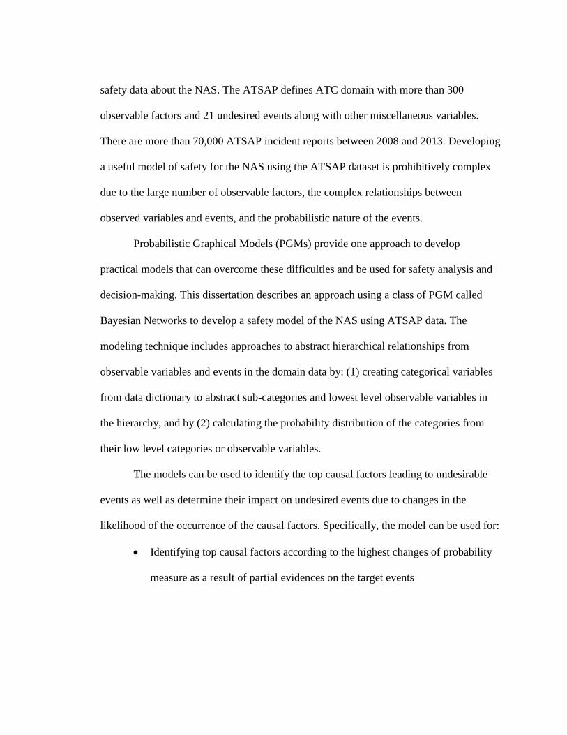
The models can be used to identify the top causal factors leading to undesirable
events as well as determine their impact on undesired events due to changes in the
likelihood of the occurrence of the causal factors. Specifically, the model can be used for:
Identifying top causal factors according to the highest changes of probability
measure as a result of partial evidences on the target events

xvi
Measuring the significance of the relationships of aggregated top causal
factors with the undesired event overtime using time series and regression
analysis
Determining correlations between top causal factors to identify sub-factors for
those factors that are difficult to act upon
Identifying top generic issues in the NAS by applying a ranking algorithm that
uses the frequency of each top causal factor and the severity index of events
This powerful tool can be used to supplement the existing decision-making
process which relies on expert judgments that are used by governments to determining
the initiatives to address safety concerns. Application of this methodology is used to
identify significant causal factors and top issues in the NAS using 41,000 records of data
from the ATSAP database from 2008 to 2013.
As demonstrated in one of the top causal factors models in this dissertation, the
probabilistic causal models can be extended into decision networks by formulating a
unified utility function using control and mitigation variables and by maximizing the
utility function. A decision network is used to help make optimum data-driven decisions
thereby reducing the likelihood of the undesired events and their consequences. This is
achieved by combining graphical, computational, and statistical software libraries and
packages.
The model outputs of the top causal factors for individual events show that 15 of
the 21undesired events can be explained with a small number of causal factors, typically
ranging from 5 to 8 sub-factors. This is in line with the yearly published report by the
xvii
“Top-5 Safety Hazard” provided by the Office of Safety at the Federal Aviation
Administration (FAA). The top issues identified in the analysis are ranked by weighting
the relative frequency of each factor and the severity of the events the factor is involved
in. The top five issues of this research’s output include individual factors (controller
actions), outside influences (distractions), clearance problems, aircraft performance, and
procedure deficiencies. Only procedural deficiencies (conflicting) and clearance
problems (heading) were reported in the Top-5 report for the year 2013. The other issues
either were not identified in the manual process or were considered non-actionable (e.g.
distractions). The analysis identified actionable sub-factors contributing to the non-
actionable causal factors (e.g. ambient noise is one of the highly correlated actionable
sub-factors identified for distractions). The analysis also identified the relationships
between top factors and relative frequencies of the undesired events and trends overtime
emphasizing the need for more careful analysis within the annual time frames as well as
year-over-year analysis.
1
1. INTRODUCTION
Probabilistic causal models, also called Bayesian networks, are used in a wide
variety of problem domains such as medicine, finance, forensic, computing, natural
sciences, engineering, and many more. The principle of Bayesian networks is based on
simple graph theory and rules of probability to represent random variables and
probability distributions. Bayesian networks provide a natural and compact representation
of probabilities by taking advantage of independencies that may exist in any problem
with uncertainty. The random variables are represented by the nodes in the graph and the
correlations and dependence of the variables are represented by the edges and local
distributions on each variable. Building Bayesian networks for problems involving
smaller number of variables is relatively simple and there are various commercial and
open source packages that are easy to use. However, problems with large number of
variables usually involve complex structures as well as large number of parameters.
1.1. Background of the Problem Safety is a vital component of aviation operation and the very survival of the
industry is entirely dependent on the safety of commercial aviation in transporting people
and goods. Few issues grab the attention of the general public and elected officials as
aviation accidents. The National Transportation Safety Board (NTSB) defines aviation
accident as an occurrence associated with the operation of an aircraft that takes place

2
between the time any person boards the aircraft with the intention of flight and the time
all such persons have disembarked, and in which any person suffers a fatal or serious
injury or the aircraft receives substantial damage.
Overall, the safety record of aviation has improved dramatically in the past many
decades, and as a result accidents occur very rarely. However, aviation operation is not
completely accident-free, and with the expected growth of flight operations in the coming
decades, the system will benefit from improved safety procedures. One of the ways of
improving aviation safety is learning from past mistakes, causes that led to accidents. But
with such small accident rates it is practically impossible to rely on the lessons learned
from past accidents to identify all possible causal factors in future potentially catastrophic
accidents. It is also not an optimal approach to wait for accidents to establish enough data
in order to prevent them in the future. Hence, since the 1970s, the aviation community
has resorted to study the causal factors of incidents and improve the system based on the
deficiencies discovered by incidents that could have become accidents with the existence
of additional factors. Most aviation operators have some kind of safety action program
through which they collect incidents from pilots, flight attendants, and maintenance
personnel for analyzing events that have the potential to lead to accidents. According to
International Civil Aviation Organization’s (ICAO) recommendation, safety reporting is
a critical component of Safety Management System (SMS). Most of these individual
safety action programs share information and have created a central data repository which
facilitate the environment to discover deficiencies in the system and make forecasts about
potentially serious accidents.
3
1.2. Air Traffic Safety Action Program (ATSAP) Data In late 2008 the FAA started ATSAP for air traffic controllers modeled after the
Aviation Safety Action Program (ASAP) run by many airlines for pilots, mechanics,
flight attendants, and dispatchers. The main objective of the program is to identify risks
in the National Airspace System (NAS) and mitigate those risks by addressing issues that
are relatively easier to fix in short time and collect historical data to be able to identify
systemic and serious issues that could result in catastrophic accidents in the long term.
ATSAP data is stored in a relational database and is comprised of structured data and
narratives. The narratives provide descriptions of events by reporters and the structured
data contain information about various categories, like event classifications, flight phases,
complexities etc. and factors that caused and/or contributed to the incident.
At the top layer of the ATSAP causal hierarchical structure there are fifteen
categories and each category is comprised of multiple level causal taxonomies. Each of
these causal entries is used to measure its causality or contribution to various undesired
events. The top causal factor categories are, 1) Individual Factors, 2) Supervisory and
Organizational Factors, 3) Fatigue, 4) ATC/Pilot Communication, 5) Coordination, 6)
Airspace and Procedures , 7) Aircraft Performance or Pilot Actions, 8) Weather, 9)
Sector, Position and Environment, 10) Equipment, 11) Training and Experience, 12)
Flight Data, Display Problems, and Aircraft Observation, 13) Airport and Surface, 14)
Emergency Situations and Special Events, and 15) Traffic Management.
Events that are captured as involving loss of separation or Traffic Proximity
issues are subdivided into, 1) Adjacent Airspace, 2) IFR to IFR (Instrument Flight Rules),
3) NMAC (Near-Mid Air Collision), 4) Runway Incursion, 5) TCAS RA (Traffic

4
Collision Avoidance System – Resolution Advisory), 6) Terrain/Obstruction, 7) VFR
(Visual Flight Rules) to IFR, 8) VFR to VFR, 9) Vehicle/Pedestrian, and 10) Wake
Turbulence. Events that occur as a result of unexpected conditions are subdivided into, 1)
Aircraft Emergency, 2) Aircraft Security, 3) Altitude, 4) Course/Routing, 5) Equipment
Issues, 6) Go Around, 7) NORDO (No Radio), 8) Speed, 9) Spillout/Whiskey Alert, and
10) Unsafe Situation. The severity, traffic complexity and other miscellaneous variables
capture various aspects of incidents. Most of the variables in ATSAP database are
categorical and hence they are more appropriate to classification algorithms such as
Bayesian networks.
There are primarily two types of problems reported by air traffic controllers,
systemic issues and safety events. Systemic issues are those that cause recurring
problems that affect the NAS such as procedures, rules, equipment, practices, conditions,
airspace design, etc. Incident reports on the other hand are filed for problems involving
one particular event or incident such as possible or actual Operational Error, Operational
Deviation, Pilot Deviation, etc. NTSB defines an incident as an occurrence, other than an
accident, associated with the operations of an aircraft which affects or could affect the
safety of operation. In loose definition, incidents are events as near-accidents and hence,
causal factors that lead to incidents lead to accidents as well. Consequently, analyzing
large number factors that lead to incidents helps to identify safety trends and proactively
take accident preventive measures.
When controllers file incident reports, analysts work on those reports to gather
additional relevant facts about the event either from the original submitter or external
5
sources for known reports. Once the analysis part is complete, issues that can be
addressed in shorter time period are resolved and the applicable causal factors are
selected for the report and archived in the database. A number of variables can be
selected as causal and/or contributing factors from multiple categories. For instance, an
incident can be caused by a combination of weather factors, communication problems,
and coordination problems; hence there exist relationships among various categories of
causal factors.
1.3. Research Scope There are various data-driven approaches to study causal factors for different
accident scenarios and their consequences which include event sequence diagrams, fault
trees, event trees, etc. This research focuses on the large number of potential causal
factors for various unwanted events in ATC operation. As there are highly interrelated
causal factors for various event types, there exists inherent uncertainty which can be
represented using probabilistic relationships among the variables.
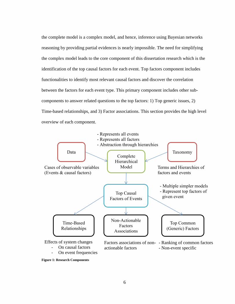
1.3.1. Research Components This research contains various independent and related components (figure-1).
The problem is defined based on the high number of factors causing and/or contributing
to various aviation events in the ATSAP dataset. The large number of factors is
abstracted using multiple levels of hierarchical structure using ATSAP taxonomy. In the
first step, a complete hierarchical probabilistic model represents all the causal factors and
events in the domain. The complete model answers two basic queries, the probability of
each event and the contribution of all factors and their high-level categories. However,
6
the complete model is a complex model, and hence, inference using Bayesian networks
reasoning by providing partial evidences is nearly impossible. The need for simplifying
the complex model leads to the core component of this dissertation research which is the
identification of the top causal factors for each event. Top factors component includes
functionalities to identify most relevant causal factors and discover the correlation
between the factors for each event type. This primary component includes other sub-
components to answer related questions to the top factors: 1) Top generic issues, 2)
Time-based relationships, and 3) Factor associations. This section provides the high level
overview of each component.
Figure 1: Research Components
Data Taxonomy Complete
Hierarchical
Model
Top Causal
Factors of Events
Time-Based
Relationships
Non-Actionable
Factors
Associations
Top Common
(Generic) Factors
Effects of system changes
- On causal factors
- On event frequencies
Factors associations of non-
actionable factors
- Ranking of common factors
- Non-event specific
Cases of observable variables
(Events & causal factors)
- Represents all events
- Represents all factors
- Abstraction through hierarchies
Terms and Hierarchies of
factors and events
- Multiple simpler models
- Represent top factors of
given event
Represents all factors
7
1.3.2. Hierarchical Abstraction of Causal Factors In many domains with large number of variables people often use categories and
hierarchies to study relationships by abstracting low level details. Similarly, to simplify
modeling safety risk in the NAS, we need categorical abstractions to analyze the large
volumes of causal factors of ATC-related aviation incidents. This research incorporates
the various level categories as defined in the data dictionary of the dataset to abstract
causal factors. The abstraction layers help study factors at higher levels which become
necessary often times when we don’t need to pay close attention to the details. For
instance, one may need to study the effect of aircraft performance in general in causing
wake turbulence events without going to the details of specific performance related issues
of different aircraft types.
1.3.3. Top Causal Factors of Events At the core of most aviation safety risk analysis is the identification of the causal
and/or contributing factors of incidents that could potentially lead to accidents. As a
complex system the NAS is exposed to various types of events that result in undesired
outcomes. This research focuses on events and causal factors that are strictly related to
ATC operation. Hence, a critical component of the research is to identify the top causal
and/or contributing factors of each ATC event from data. In ATSAP dataset there are
more than three hundred causal factors that play a significant role in causing ATC related
aviation events. However, for the purpose of safety assessment, it is nearly impossible to
focus on all these factors. So, the goal of this part of the research is to algorithmically
determine the causal factors that are responsible for the majority of individual events. By
isolating the factors that are primary contributors to safety issues, it becomes possible to
8
focus on smaller but critical issues that can be studied and addressed reasonably
efficiently with the limited resources available. The methodologies section will cover the
details of the algorithm as to how the top factors are selected.
1.3.4. Common/Generic Safety Factors Isolating the causal factors of individual events are important in a sense that
occasionally, we focus on specific aviation events such as loss of separation, runway
incursion, operation deviation etc. to study them in detail and understand why they occur.
However, the primary goal of safety management is to minimize the risk in the NAS from
any kind of potential aviation accident. So, the study of generic aviation issues, regardless
of what type of event they are likely to lead to, is a critical piece of safety assessment.
The Air Traffic Organization (ATO) office of safety at the FAA has a program called
Top-5 Hazard that is responsible to publish the five significant ATC related issues every
year. Although some of the methods followed in the identification process are not backed
by sound mathematical approaches, the fact that there is a responsible and dedicated party
to isolate those few issues is critical. This research introduces an algorithm that ranks the
top causal factors identified for all ATC events into generic ATC related factors based on
the relative frequency and the severity classification of every event that the factors are
associated with.
1.3.5. Relationships of Causal Factors At times, we need to deal with factors that are highly impactful in causing events
but are difficult or impossible to directly tackle. A real example of such issues is a duty
related distraction, which according to the result of this research is the fifth top issue in
9
causing various ATC related aviation events in the last two years. However, there is little
one can do to directly affect the impact of duty related distraction issues. So, the
approach introduced in this research is to treat such factors individually as target
variables and explore other causal factors that have significant correlation with them. The
intuition is by acting on other strongly correlated factors the effect of the target causal
factor can be reduced thereby minimizing the likelihood of those events that are caused
by non-actionable factors.
1.3.6. Decision Analysis Incorporating a decision optimization mechanism to a safety risk assessment is an
important component and adds another layer of analysis to the factor identification
process to make a better decision on the outcome of the probabilistic models. The
ultimate goal of identification of issues and causal factors is to intervene in the system by
taking actions to change the natural course of events, that is, to minimize the probability
of the occurrence of undesired outcomes in the NAS. However, the mere identification
process doesn’t give us the means by which we make the optimum decisions. It doesn’t
answer questions like which factors to resolve first, how many factors to deal with, and
which combinations of fixes give rise to the optimum result, both in terms of safety
impact and resource allocation. Decision analysis will enable us to efficiently pick the
right issues to work on with the amount of resources we have. In this research, I
demonstrate a decision network based on three top causal factors of a runway incursion
problem. There are some assumptions that I make since some of the data points required
for such analysis is not available in the dataset used for this research.

10
1.3.7. Summary of Research The list in table-1 below summarizes the existing challenges and the solutions
suggested in this research to each problem.
Table 1: Summary of Research
Item Problem Solution
1 As attributes of a complex system,
the causal factors of aviation events
are abstracted through hierarchies
and categories. How do you
represent such abstractions in
probabilistic models?
Represent the categories as regular
variables and encode them in the
models and calculate their
probabilities from their low level
counterparts which are directly
observable.
2 Of the large number of attributes in
the NAS, what are the top factors
that are causal and/or contributory
to various aviation events?
Identify small number of top causal
factors that are responsible for the
large majority of events using a
probabilistic approach.
3 The ultimate goal of aviation safety
is to make the NAS a safer system,
not studying individual events.
What are the top common issues in
the NAS regardless of their
association to various event types?
Using the top causal factors identified
for various events, apply a ranking
algorithm based on frequency and
severity in order to determine the
contribution of factors in causing
events.
4 The NAS is a dynamic
environment, hence, factors
affecting its operation change over
time. How do you determine the
change of the effect of some factors
on events over a period of time?
For factors and issues identified as
causal and/or contributory for various
events, calculate the relationship of
their aggregates with the frequency of
the target event and determine their
impact overtime.
3 Some factors are non-actionable,
that is, no direct resolution is
available. How do you approach
such issues?
Treat them as target variables and
identify other causal factors that have
strong correlations. By resolving
those factors it is more likely the
target factors are affected indirectly.
6 Probabilistic modeling for complex
system is difficult in general, even
with the help of software packages.
Can the process be fully automated?
Design an automation program that
represent various parameters and
build models with little manual
intervention by merging various
packages and custom code
11
1.4. Why Probabilistic Reasoning? Until recent decades, the Artificial Intelligence (AI) community had not embraced
probabilistic reasoning as a paradigm to deal with problems involving uncertain set of
evidences or incomplete information. The driving theme in the 1960s and 1970s in most
AI projects was that logic can fully represent knowledge and the reasoning within.
However, most expert systems needed a mechanism to deal with the inherent uncertainty
that results from ambiguous concepts and/or simple lack of complete evidence which
may not be represented fully with logic. With the advent of naïve Bayes in medical
diagnosis, it became possible to encode probability in AI programming although the
strong assumption of independence extremely limited the scope of applying naïve Bayes
in many complex problems. As computational power increased significantly it was
possible to represent uncertainty with probability without the constraints of strong
independence assumptions. Bayesian networks are one of such systems to encode
uncertainty in many problem domains, they are representations of the probabilistic
relationships among a set of variables, and they have gotten a wide acceptance in the
larger AI community.
The application of probabilistic reasoning as a classification and predictive
modeling tool may be dictated by various requirements and objectives in the domain. In
general probabilistic reasoning using graphical models provides the encoding of
uncertainties using probabilities and the compact representation of complex joint
distributions. This section summarizes the benefits of applying probabilistic reasoning for
modeling aviation risk and analyzing incidents data.
12
1.4.1. Role of Uncertainty In any given domain with some level of complexities, there are many sources of
uncertainties, the complex interaction of observable and unobservable variables,
ambiguous concepts, lack of knowledge in some areas, human subjectivity, and the
limitation of our models. So, most models representing a real world scenario have to deal
with uncertainties to various degrees. As this research project focuses on one of the most
complex systems available, it deals with uncertainty in a number of areas. Modeling the
ATC-related aspects of the NAS involves various level of uncertainties based the specific
area of application such as the interaction of causal factors, the severity of events, the
dynamic nature of the NAS etc. Therefore, probabilistic reasoning is the most appropriate
analytical approach to assess and represent those uncertain relationships among various
components.
1.4.2. Compact Representation of Complex Structure At the very basic level, a probabilistic model is about compact representation of
joint distributions. The complexity of modeling joint distribution increases exponentially
with the number of variables. Assumption of absolute independence among all variables
makes the space and time complexity easier to deal with, but such strong assumptions are
rarely satisfied for any real world problem and not suitable in most cases. The alternative
is a relative independence assumption by involving conditional probability. Applying
such weaker assumptions, probabilistic models can represent the full joint distribution of
most real world problems compactly with reasonable accuracy. Air traffic operation in
the NAS involves many variables, and without some level of independence assumptions,
it is extremely difficult to model the full joint distribution.
13
1.4.3. Extension to Decision Networks Probabilistic graphical tools are used to model either simple correlations or
causations and make probabilistic inference using the knowledge base in the model.
However, standard Bayesian networks cannot be used for decision analysis. A decision
network is a generalization of a Bayesian network by incorporating one or more expected
utility functions. By maximizing expected utility functions, a decision network becomes a
natural extension of Bayesian networks and can be used to help make optimum decisions.
Many of the challenges in ATC operations involve making decisions to make changes to
existing systems and introducing new technological solutions, procedural, and/or policy
changes with minimum disruption to the system as a whole. By extending the various
probabilistic causal model outputs in this research to decision networks in future work,
critical decision making processes can be enhanced following a data-driven approach.
1.5. Application in Other Domains The methodologies used and the approaches introduced in this dissertation are
applied on aviation incident data as a research case study. However, they can equally be
applied for problems in other domains that have similar characteristics. The core of this
research is the introduction of a feature selection algorithm using a Bayesian network
principle iteratively. Specifically, a smaller subset of features (causal factors) is selected
for each event type of ATC-related aviation incidents from a large set of factors. The
purpose of the feature selection algorithm in this research is simplifying the problem by
reducing the dimension and improving the prediction performance of the classification of
the target variables. Although the features selected in the case study for this research
involve only causal factors, the algorithm can equally work for non-causal predictors.

14
As described in section 3.3, the two-phased selection algorithm introduced in this
research include independent ranking of the factors followed by a selection process using
evidence propagation of Bayesian networks. The first step involves ranking all the
available features using a sensitivity analysis based on the difference of prior and
posterior probabilities. In the second phase, multiple Bayesian networks with increasing
number of features are created iteratively and the process stops when the gain in the
reduction of the Brier score, a probabilistic prediction metric, is smaller than the gain in
the previous iteration. The final probabilistic network will contain only the significant
features for classifying or predicting the target variable. In this approach, the ranking
phase is an independent preprocessing step for filtering the large number of features.
Hence, it is a step that ranks features according to their individual predictive power based
on conditional probability. Due to its individual treatment, this approach may be prone to
selecting redundant features.
For relevant feature Fi, other feature Ci, and target event Ei, the following
probability relation holds.
( | ) ( | )
One area in healthcare domain where this selection algorithm can be used is for
diagnosis of a disease. A set of test cases may be used to select features that can predict
the existence of a heart disease, for instance. The factors in such kind of feature selection
may or may not be causal factors as their type is irrelevant for the mere purpose of
predicting the disease. To select a subset of factors from a large set that can be used to
diagnose a heart disease, in the first step, all the causal factors are ranked independently

15
using the difference of the prior and posterior probabilities. In the second phase, multiple
Bayesian networks are learned incrementally by including factors to the probabilistic
network, one at a time, according to their rank until the gain in the reduction of the Brier
Score (BS), a probabilistic accuracy metric, starts decreasing. When the current BS
reduction gain is smaller than the one in the previous iteration, the probabilistic network
learning process is stopped and the factors that have become part of the structure in the
network are the relevant factors that can be used to diagnose the disease.
All the other algorithms that are part of this research are based on the core
selection algorithm, i.e. they are extensions of the identification of the significant factors.
The generic top factors, (section 3.5), are the re-ranking of all the selected factors based
on frequency and severity index. As a result, they can be used in other domains as well,
for instance, significant factor for cancer as opposed to a specific type of cancer (e.g.
prostate cancer). Similarly, the time-based relationships, (section 3.6), can be applied in
any problem with a dynamic environment in which there is a potential for relationship
changes as a function of other external factors.
16
2. LITERATURE REVIEW
Many data-driven research projects involve some level of modeling, usually based
on statistical principles. Similarly, safety risk analyses in general are mostly done with
the help of models. Graphical models have the added benefits of presenting the output
using visualization tools that can appeal to the human eye. Although there are various
graphical tools for the aviation safety professional, Bayesian networks for risk analysis
are becoming popular. However, most Bayesian modeling in aviation risk analysis are
done using expert judgment due to immaturity of model learning algorithms and data
availability. Some graphical tools in use today and few of the data-driven research works
that have some resemblance to this research project are explained in this section.
2.1. Common Models and Tools in Aviation Risk Analysis Aviation operation is realized by the complex interactions of technical and
organizational systems which also contribute to the failure of this operation at times.
Hence, models to represent such systems need to simulate the complexity of those
interactions. There are various visual or graphical models that are widely used in aviation
risk analysis. Each has strengths and weaknesses and is applied in different scenarios of
risk assessment and visualization of safety hazards. Below is a short survey of the models
and visual tools that are commonly used in aviation safety analysis.
17
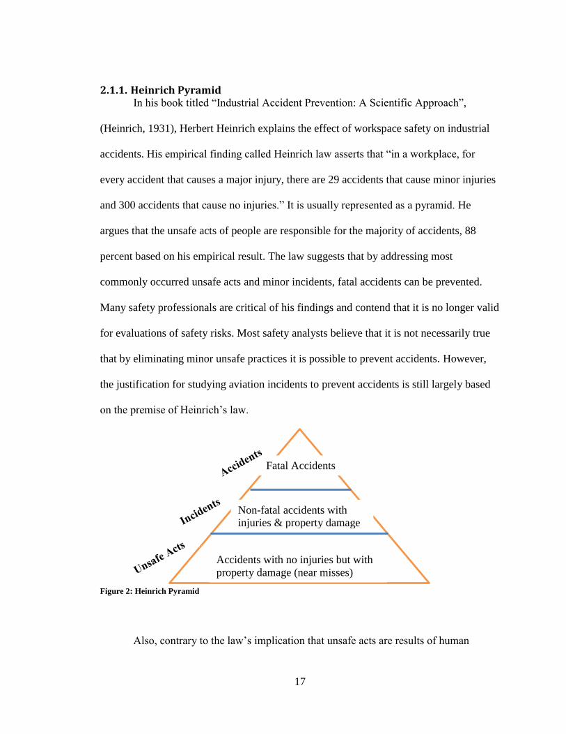
2.1.1. Heinrich Pyramid In his book titled “Industrial Accident Prevention: A Scientific Approach”,
(Heinrich, 1931), Herbert Heinrich explains the effect of workspace safety on industrial
accidents. His empirical finding called Heinrich law asserts that “in a workplace, for
every accident that causes a major injury, there are 29 accidents that cause minor injuries
and 300 accidents that cause no injuries.” It is usually represented as a pyramid. He
argues that the unsafe acts of people are responsible for the majority of accidents, 88
percent based on his empirical result. The law suggests that by addressing most
commonly occurred unsafe acts and minor incidents, fatal accidents can be prevented.
Many safety professionals are critical of his findings and contend that it is no longer valid
for evaluations of safety risks. Most safety analysts believe that it is not necessarily true
that by eliminating minor unsafe practices it is possible to prevent accidents. However,
the justification for studying aviation incidents to prevent accidents is still largely based
on the premise of Heinrich’s law.
Figure 2: Heinrich Pyramid
Also, contrary to the law’s implication that unsafe acts are results of human
Non-fatal accidents with
injuries & property damage
Accidents with no injuries but with
property damage (near misses)
Fatal Accidents
18
errors, it is widely accepted that system designs and other environmental variables are
more responsible for unsafe acts in the workplace.
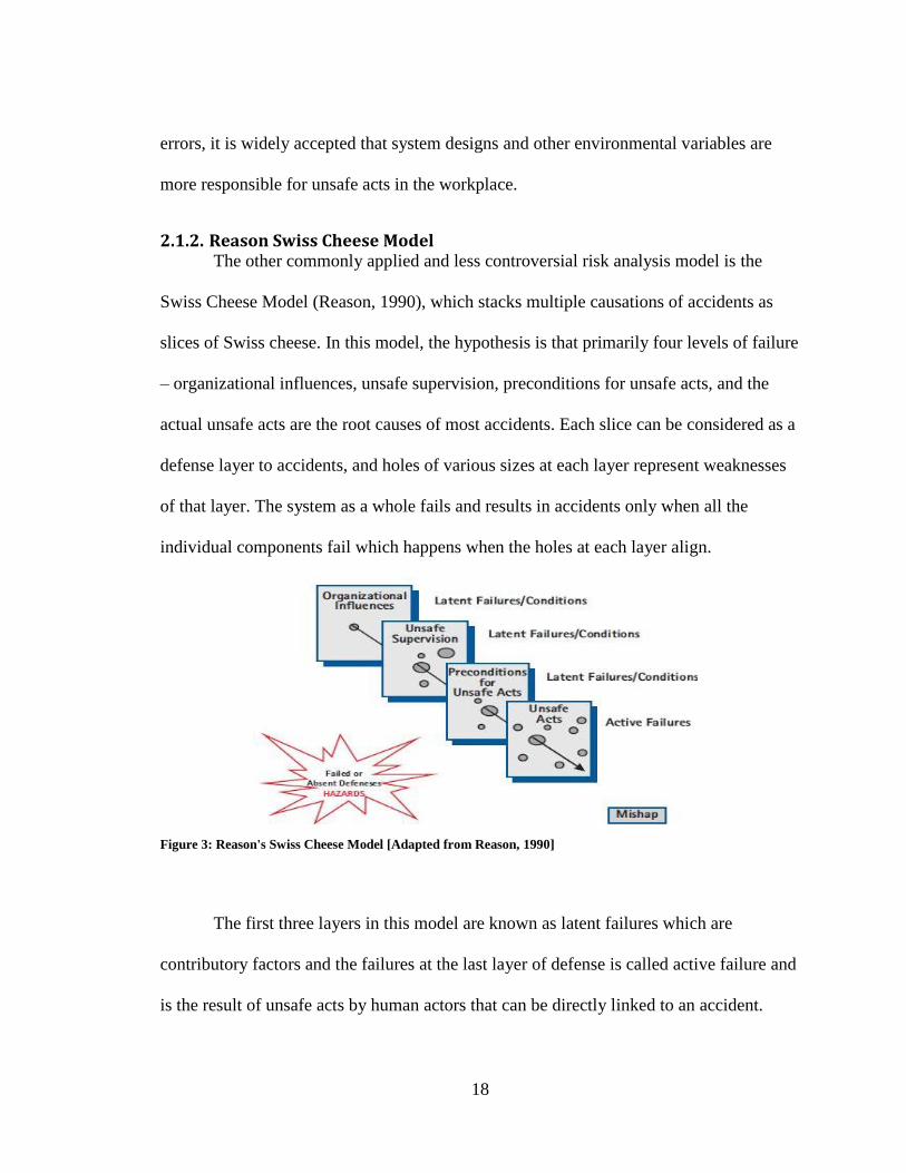
2.1.2. Reason Swiss Cheese Model The other commonly applied and less controversial risk analysis model is the
Swiss Cheese Model (Reason, 1990), which stacks multiple causations of accidents as
slices of Swiss cheese. In this model, the hypothesis is that primarily four levels of failure
– organizational influences, unsafe supervision, preconditions for unsafe acts, and the
actual unsafe acts are the root causes of most accidents. Each slice can be considered as a
defense layer to accidents, and holes of various sizes at each layer represent weaknesses
of that layer. The system as a whole fails and results in accidents only when all the
individual components fail which happens when the holes at each layer align.
Figure 3: Reason's Swiss Cheese Model [Adapted from Reason, 1990]
The first three layers in this model are known as latent failures which are
contributory factors and the failures at the last layer of defense is called active failure and
is the result of unsafe acts by human actors that can be directly linked to an accident.
19
One obvious limitations of this model is that it doesn’t look at the interactions among the
four levels; instead it models the barrier at each layer and their weaknesses without
regard to the possible effect of one layer on the other.
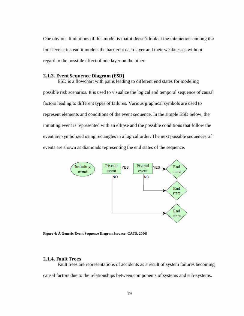
2.1.3. Event Sequence Diagram (ESD) ESD is a flowchart with paths leading to different end states for modeling
possible risk scenarios. It is used to visualize the logical and temporal sequence of causal
factors leading to different types of failures. Various graphical symbols are used to
represent elements and conditions of the event sequence. In the simple ESD below, the
initiating event is represented with an ellipse and the possible conditions that follow the
event are symbolized using rectangles in a logical order. The next possible sequences of
events are shown as diamonds representing the end states of the sequence.
Figure 4: A Generic Event Sequence Diagram [source: CATS, 2006]
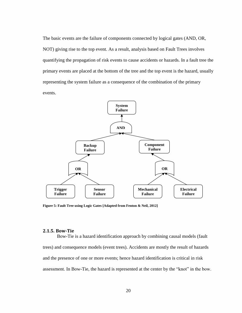
2.1.4. Fault Trees Fault trees are representations of accidents as a result of system failures becoming
causal factors due to the relationships between components of systems and sub-systems.
20
The basic events are the failure of components connected by logical gates (AND, OR,
NOT) giving rise to the top event. As a result, analysis based on Fault Trees involves
quantifying the propagation of risk events to cause accidents or hazards. In a fault tree the
primary events are placed at the bottom of the tree and the top event is the hazard, usually
representing the system failure as a consequence of the combination of the primary
events.
Figure 5: Fault Tree using Logic Gates [Adapted from Fenton & Neil, 2012]
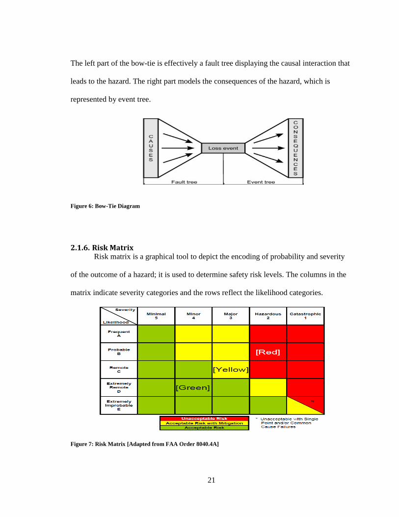
2.1.5. Bow-Tie Bow-Tie is a hazard identification approach by combining causal models (fault
trees) and consequence models (event trees). Accidents are mostly the result of hazards
and the presence of one or more events; hence hazard identification is critical in risk
assessment. In Bow-Tie, the hazard is represented at the center by the “knot” in the bow.
AND
OR
System
Failure
Backup
Failure
Component
Failure
Sensor
Failure
Trigger
Failure
Mechanical
Failure
Electrical
Failure
OR
21
The left part of the bow-tie is effectively a fault tree displaying the causal interaction that
leads to the hazard. The right part models the consequences of the hazard, which is
represented by event tree.
Figure 6: Bow-Tie Diagram
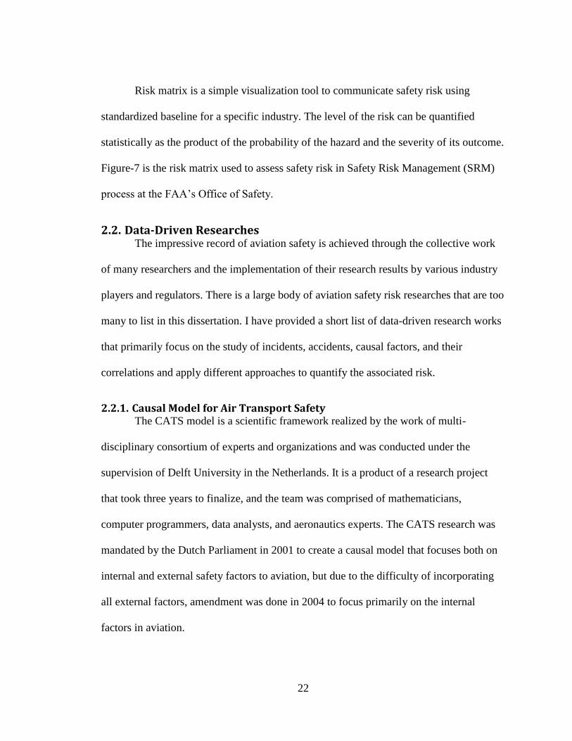
2.1.6. Risk Matrix Risk matrix is a graphical tool to depict the encoding of probability and severity
of the outcome of a hazard; it is used to determine safety risk levels. The columns in the
matrix indicate severity categories and the rows reflect the likelihood categories.
Figure 7: Risk Matrix [Adapted from FAA Order 8040.4A]
22
Risk matrix is a simple visualization tool to communicate safety risk using
standardized baseline for a specific industry. The level of the risk can be quantified
statistically as the product of the probability of the hazard and the severity of its outcome.
Figure-7 is the risk matrix used to assess safety risk in Safety Risk Management (SRM)
process at the FAA’s Office of Safety.
2.2. Data-Driven Researches The impressive record of aviation safety is achieved through the collective work
of many researchers and the implementation of their research results by various industry
players and regulators. There is a large body of aviation safety risk researches that are too
many to list in this dissertation. I have provided a short list of data-driven research works
that primarily focus on the study of incidents, accidents, causal factors, and their
correlations and apply different approaches to quantify the associated risk.
2.2.1. Causal Model for Air Transport Safety The CATS model is a scientific framework realized by the work of multi-
disciplinary consortium of experts and organizations and was conducted under the
supervision of Delft University in the Netherlands. It is a product of a research project
that took three years to finalize, and the team was comprised of mathematicians,
computer programmers, data analysts, and aeronautics experts. The CATS research was
mandated by the Dutch Parliament in 2001 to create a causal model that focuses both on
internal and external safety factors to aviation, but due to the difficulty of incorporating
all external factors, amendment was done in 2004 to focus primarily on the internal
factors in aviation.

23
One of the justifications for causal models, the researchers argue, is that
traditional analytical methods are no longer able to deal with systems whose degree of
complexity are at the level of aviation’s. The CATS model provides the capabilities to get
into the cause-effect relationships of incidents and accidents and enables risk assessment
quantitatively as well as the mechanism to measure mitigation of risk.
2.2.1.1. Overview Different categories of aviation accidents are direct consequences of the complex
interactions of various causal factors the severity of which depend on the specific phase
of flight in which they occur. The CATS project approaches this complexity based on the
accident categories in different flight phases by representing them in separate Event
Sequence Diagrams and Fault Trees and converting the individual models into one
integrated Bayesian Belief Network (BBN). As a result, the CATS model can deal with
causal factors as well as consequences of accidents, but the authors suggest giving
emphasis on the causal factors, hence the name. Unlike fault trees and event trees which
are inherently deterministic, the final output of CATS model, as a BBN-represented
mathematical tool, is the probability of an accident as calculated from the various
probabilistic relationships of the causal factors. The causal factors include interactions
between systems and people who operate and maintain the systems: controllers, pilots,
and maintenance personnel.
2.2.1.2. Data and Expert Judgment The researchers have used both data, when available, and expert judgment to
build the CATS model. They primarily used ICAO’s Accident/Incident Data Reporting

24
System (ADREP) database whose main sources are airlines and airports of member states
and Airclaims which is a data source of aviation claims. They also used Line Operations
Safety Audit (LOSA) data, which are data collected from a voluntary formal process that
uses trained observers to collect safety-related information on regular basis to establish
performance of cockpit crews.
2.2.1.3. Methodology The CATS model consists of a number of programs, UNINET, a Bayesian
software package to perform mathematical operations in the quantification process,
UNISENS, to perform statistical analyses, UNIGRAPH, to display the BBN, and
database management tools. The CATS research project was built upon a previous
research work done in the area of occupational safety, associating technological risks to
management influences. The product of this work is a model comprising of three
modeling techniques, Event Sequence Diagrams (ESD), Fault Trees (FT), and Bayesian
Belief Nets (BBN). The ESDs are used to model the various potential accident categories
along with their causal factors using the taxonomy adopted in ADREP. The ESDs are
divided according to flight phases such as Taxi, Take-Off, Climb, en route, and Approach
and Landing. In the final CATS model 33 ESDs are incorporated.
25
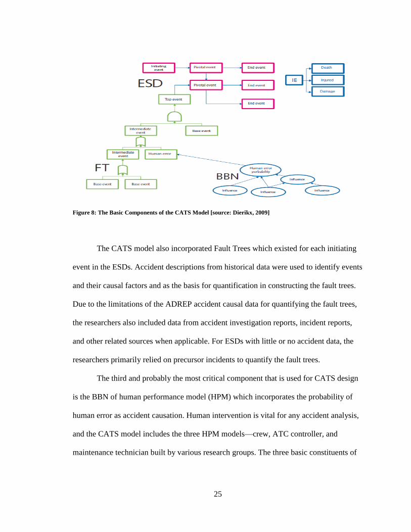
Figure 8: The Basic Components of the CATS Model [source: Dierikx, 2009]
The CATS model also incorporated Fault Trees which existed for each initiating
event in the ESDs. Accident descriptions from historical data were used to identify events
and their causal factors and as the basis for quantification in constructing the fault trees.
Due to the limitations of the ADREP accident causal data for quantifying the fault trees,
the researchers also included data from accident investigation reports, incident reports,
and other related sources when applicable. For ESDs with little or no accident data, the
researchers primarily relied on precursor incidents to quantify the fault trees.
The third and probably the most critical component that is used for CATS design
is the BBN of human performance model (HPM) which incorporates the probability of
human error as accident causation. Human intervention is vital for any accident analysis,
and the CATS model includes the three HPM models—crew, ATC controller, and
maintenance technician built by various research groups. The three basic constituents of
26
the CATS model are depicted in a single integrated model as shown in the figure-8
above.
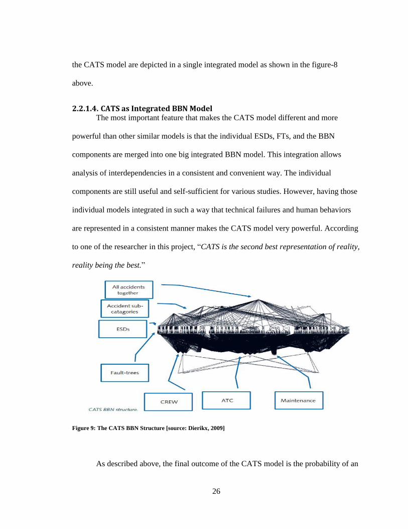
2.2.1.4. CATS as Integrated BBN Model The most important feature that makes the CATS model different and more
powerful than other similar models is that the individual ESDs, FTs, and the BBN
components are merged into one big integrated BBN model. This integration allows
analysis of interdependencies in a consistent and convenient way. The individual
components are still useful and self-sufficient for various studies. However, having those
individual models integrated in such a way that technical failures and human behaviors
are represented in a consistent manner makes the CATS model very powerful. According
to one of the researcher in this project, “CATS is the second best representation of reality,
reality being the best.”
Figure 9: The CATS BBN Structure [source: Dierikx, 2009]
As described above, the final outcome of the CATS model is the probability of an
27
accident as a result of the interaction between various components. The final model has
1400 nodes and 5000 arcs representing 33 accident scenarios and 1200 initial and
intermediate events associated with these accidents, the network is shown in figure-9.
The reader is referred to the CATS report to fully understand the principles of the
conversion process and the detail mathematical operations the research team followed to
quantify risk in various accident categories.
2.2.1.5. Observation The main strength of the CATS model is the integration of various dependencies
of causal and contributing factors to measure probability of accidents which makes it
closer to reality. The model makes it possible to investigate various scenarios by varying
parameters that maybe difficult in real life. The research team of the CATS model relied
heavily on expert judgment to quantify the human performance model, so one needs to
exercise caution when analyzing the human error aspect of safety risk using this model.
For instance, maintenance crew’s model is equally represented in the model as flight-
crews and air traffic controllers, but in reality the maintenance technician can, for the
most part, affect accidents indirectly. One important improvement that can be done in
CATS model, especially in areas where experiment judgment is heavily used, is to do
validation work by finding related data or simulated data or apply part of the model in
other industries where data can be found relatively easily.
2.2.2. Modeling Aviation Risk (ASRM) ASRM is a product as well as a process; it is developed with joint support from
the National Aeronautics and Space Administration (NASA) and the FAA and primarily
28
intended for “low probability-high consequence (LP/HC)” events. LP/HC events are
characterized by consequences of low likelihoods, high severity and they are ill-
structured and result from multi-layered causal and contributing factors. Due to the
limitations of common analytical risk methods, such as fault trees, event trees, event
sequence diagrams, the team designed Bayesian Network-based solution that enables to
analyze multiple causalities in an integrated and systematic fashion. Using this approach
the authors claim that precursors to aviation incidents can be identified.
2.2.2.1. Methodology As a Bayesian approach, the authors represent precursors as nodes and the arcs
represent the relationships between causal factors. Interventions in the form of
technology are represented by decision nodes. The authors used the Hugin Bayesian
networks inference algorithm and programming tool.
So as to measure aviation accident risk, ASRM aggregates ideas and concepts
regarding aircraft accident causal and contributing factors. As a process, ASRM lays out
procedures as to how multi-layered precursors can be studied together along with
interventions to assess their effects in causing accidents. As a product, multiple ASRM
models were developed based on cases of specific aviation accidents. In these models, the
probabilistic interdependencies of organizational, individual, task/environmental factors
are analyzed in relation to aircraft accidents in a structured approach and risk assessments
are performed by measuring the likelihood and severity of aviation accidents. A total of
twenty models have been developed at Rutgers University as part of this project for six
types of aircraft accidents, such as controlled flight into terrain, loss of control, runway
29
incursion, engine failure, maintenance, and general aviation. The models were generated
both using case studies and elicitation of expert opinions. Thirty subject matter experts
participated for training the models. Below are the systematic steps the researchers
followed to create the risk models for various accident types,
Selecting and analyzing a real accident case
Identifying the case-based causal factors
Constructing the diagram of the causal factor correlations
Building the Bayesian Believe Network (BBN)
Inserting technologies/interventions
Evaluating relative risk
ASRM researchers identified causal factors from accident reports and used the
Human Factors Analysis and Classification System (HFACS) as developed by Weigmann
and Shappell (2003). HFACS taxonomy follows the Reason (1995) accident causation
framework, and primarily focuses on human and organizational error modeling. In
addition, ASRM included operational and equipment factors when applicable for the
accident type in the model.
After the correlation of the causal factors have been established, the conditional
probability tables are populated from the “beliefs” of subject matter experts by
establishing boundary conditions such as a towered airport, moderate traffic density, time
period, etc. The Subject Matter Experts (SMEs) have also assessed the impact of one or
more newly introduced technologies on the causal factors in the form of conditional
probabilities.
30
2.2.2.2. Observation A significant contribution of this research and the ASRM process is the
assessment of relative safety risk. The software prototype from this research can be used
to evaluate various technological solutions in reducing risk by affecting causal factors for
any specific type of accident, which can serve as a decision making tool. One of the
limitations of the ASRM process is that it follows a reactive approach; it identifies causal
factors from actual accident. Also, similar to other Bayesian belief network solutions, it
relies heavily on expert judgment to identify causal factors.
2.2.3. Relationships between Aircraft Accidents and Incidents This is a research work done by Nazeri, Donohue, and Sherry in 2008 at George
Mason University. In this research the authors employed a data mining technique to
analyze factors (primary and contributory) that lead to incidents in relations to accidents.
Accidents are occurrences associated with aircraft operations in which people suffer
death or injury, and/or involved aircraft damage. Incidents are safety hazards which, with
the presence of one or more factors, could have resulted in accidents. Accidents are rare
events, and hence it is difficult to infer causal patterns from accidents alone. As a result
most data-driven aviation safety researches should involve some form of incident
analysis. Figure-8 shows annual rates of accidents which are filtered for this study based
on the authors selection criteria (source of data: NTSB).
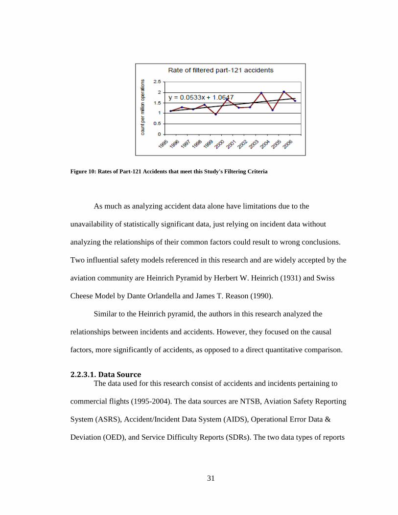
31
Figure 10: Rates of Part-121 Accidents that meet this Study's Filtering Criteria
As much as analyzing accident data alone have limitations due to the
unavailability of statistically significant data, just relying on incident data without
analyzing the relationships of their common factors could result to wrong conclusions.
Two influential safety models referenced in this research and are widely accepted by the
aviation community are Heinrich Pyramid by Herbert W. Heinrich (1931) and Swiss
Cheese Model by Dante Orlandella and James T. Reason (1990).
Similar to the Heinrich pyramid, the authors in this research analyzed the
relationships between incidents and accidents. However, they focused on the causal
factors, more significantly of accidents, as opposed to a direct quantitative comparison.
2.2.3.1. Data Source The data used for this research consist of accidents and incidents pertaining to
commercial flights (1995-2004). The data sources are NTSB, Aviation Safety Reporting
System (ASRS), Accident/Incident Data System (AIDS), Operational Error Data &
Deviation (OED), and Service Difficulty Reports (SDRs). The two data types of reports

32
are structured and event narratives. They filtered out events which are not direct results of
the operation such as medical and alcohol related events, terrorism, bird strikes, and
incidents during non-flight phases as well as incidents in the Alaska region. Some of the
limitations in such sources of data are the potential bias from self-reporting and the
underrepresentation caused by unreported events.
2.2.3.2. Methodology The authors followed a three step process to identify causal factors that are
common between accidents and incidents. First they followed a data-driven methodology
to identify common factors and sorted them into a hierarchy of factors and sub-factors
across the databases and represented them in vectors. The factors are Aircraft, Airport,
Air Traffic Control, Company, Maintenance, Pilot, Weather, and Other. Each of the
categories except “Other” has also multiple-sub categories.
Second they applied Search and Testing for Understandable Consistent Contrasts
(STUCCO) algorithm to analyze the vectors of the common factors in incident and
accident groups. STUCOO algorithm detects differences between contrasting groups
automatically from data by seeking conjunctions of attributes and values that have
different levels of support (frequency count) in multiple groups. The attributes-values
pairs are used to indicate the presence or absence of factors in each event group. The
support of the factor-set in each groups are used to calculate the deviation which in turn,
based on the minimum threshold value of 1%, is used to proceed to the next step for
further testing. Then the authors run Chi Square tests for significance of factor-set
distribution over the two groups, a p-value of 0.05 is used as a threshold.
33
Finally, they ranked the significant factor-sets based on the Factor Support Ratio
measure as follows.
( )
( )
While the deviation measures the difference between the support of the factor-set
in accident and incident groups, the support ratio measures the ratio of the probability of
a factor-set being involved in accident to its probability in incident. As a result, the
support ratio is used to compare the likelihood of a factor-set’s involvement in accident
and incident.
2.2.3.3. Results The research shows that when factors co-occur they tend to result more in
accidents based on the likelihood calculated from the support ratio. Company factors,
which include mistakes by airlines personnel, non-optimal company procedures, lack of
management etc., are identified as the highest ranked accident factors of all the factors
considered in this research. ATC factors are the next highest ranked factors,
communication issues, such as readback problem and exchange of traffic advisory and
weather information, being the most common sub-factors. Pilot factors, of which visual
lookout is the most frequent, are identified as most occurring both in accidents and
incidents which decreases their overall support ratio. Aircraft factors, which primarily
include the system of the aircraft and their performances, are identified as incident factors
unless combined with other factors. The authors conclude that based on additional study
of ten-year historical databases, pilot and aircraft factors are decreasing while ATC
factors are on the rise. Based on such trend, projections of younger ATC workforce

34
replacing exiting controllers, and the likelihood of ATC factors involvement in accidents
in this research, they argue that there is the potential of accident increase unless
additional measures are taken.
2.2.3.4. Observation The research is a data-driven approach and follows a sound method involving
statistical test. This study can serve as additional evidence as to the existence of
relationships between factors involving incidents and that of accidents. The conclusion of
this research is also similar to some other studies which investigated relationships
between aviation incidents and accidents. Some of the limitations of the research as
pointed out by the authors are, it didn’t include some large and popular databases. For
instance, ASAP is a program run by almost all commercial airlines and has a large data
repository. Including ASAP data will definitely provide more insights about causal factor
relationships. Also, due to the unavailability of data, this study is limited only to
commercial flights even though most accidents occur in general aviation. Another
limitation in this research is that causal factors are broadly categorized without regard to
the type of incident/accident involved and the severity of the event which are two
important parameters in order to use the relation of the causal factors to mitigate risk
events.
2.2.4. Other Data-Driven Researches in Aviation Safety Other researches that have some level of similarities in their objectives to this
research, which is the analysis of incidents and accidents data to identify causal factors in
35
order to determine the likelihood of the occurrence of future aviation accident, are as
follows.
Nazeri (2007) identified the relationship between incidents and aircraft accidents
through common causal factors based on cross-database analysis. Neil, Malcolm, & Shaw
(2003) showed the process of constructing Bayesian Belief Networks for ATC operations
ranging from airspace design to the operation of aircraft safety net features to a potential
accident. Motevalli & Sakata (2005) enumerated all the milestone accidents in aviation
safety from 1998 through 2020 which led to significant changes in technology, policy,
and regulations as reactive solutions as opposed to a proactive one. Marsh & Bearfield
(2007) demonstrated how to fully represent multiple quantitative risk models, such as
fault trees, using Bayesian networks by applying a case-based approach. Kardes &
Luxhøj applied hierarchical approach to Bayesian networks to model general aviation
system risk. In this research, the authors provide a meaningful hierarchical representation
of the Reason model, which contends that there exists interactions among individual
factors and latent factors, based on aircraft accident cases.
2.3. Theoretical Background This section briefly covers the principles and mathematical theories upon which
probabilistic graphical models are founded. Bayesian networks have become a major
discipline of study in the larger artificial intelligence domain and it is beyond the scope of
this research to cover the wide arrays of causal models and their exact and approximate
learning algorithms that have been discovered over the years.
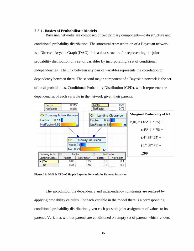
36
2.3.1. Basics of Probabilistic Models Bayesian networks are composed of two primary components—data structure and
conditional probability distribution. The structural representation of a Bayesian network
is a Directed Acyclic Graph (DAG). It is a data structure for representing the joint
probability distribution of a set of variables by incorporating a set of conditional
independencies. The link between any pair of variables represents the correlation or
dependency between them. The second major component of a Bayesian network is the set
of local probabilities, Conditional Probability Distribution (CPD), which represents the
dependencies of each variable in the network given their parents.
Figure 11: DAG & CPD of Simple Bayesian Network for Runway Incursion
The encoding of the dependency and independency constraints are realized by
applying probability calculus. For each variable in the model there is a corresponding
conditional probability distribution given each possible joint assignment of values to its
parents. Variables without parents are conditioned on empty set of parents which renders
Marginal Probability of RI
P(RI) = (.65*.11*.25) +
(.45*.11*.75) +
(.4*.88*.25) +
(.1*.88*.75) =
.209
37
unconditional probability distribution (marginal distribution). The formal definition of a
Bayesian network for variables is a pair of (G, ϴ), where
- G is a directed acyclic graph over (structure) and
- ϴ is the set of CPDs, one for each variable in (parameters)
2.3.2. Random Variables and Probability Calculus In DAG, the nodes represent random variables which can be discrete such as
severity = (Minor, Major, Hazardous) or continuous such as wind speed. In the majority
of cases Bayesian networks are used to model probability distribution on discrete random
variables. Even when they are used to model continues variables, they are usually applied
by discretization, for instance, wind speed can be grouped into ranges such as 0-5, 6-10,
11-15 knots etc. The nodes can also represent functional variables which are defined as a
function of their parent variables.
There are two contending interpretations in practical application of probability;
“Frequentist probability” and “Bayesian probability”. In the frequentist (objectivist)
interpretation, probability is a random process which denotes a relative frequency of the
outcome of an experiment while Bayesian (subjectivist) assigns a degree of belief to an
outcome as a probability. For learning the parameters in this dissertation I will use the
frequentist approach mainly because the analysis is largely a data-driven one, no
elicitation of opinion from domain experts will be incorporated for the purpose of
determining probabilities of random variables. Formal theory of probability definitions
satisfies the following properties.
For discrete probability distributions,
38
( ) [ ]
∑ ( ) Where,
- Ω is the sample space and
- f(x) is a probability mass function mapping a point in the sample space to a
probability value
For continuous probability distributions,
( )
∫ ( )
( ) ( ) ∫ ( )
Where,
- f(x) is probability density function and
- F(x) is cumulative distribution function
2.3.3. Parameterization of Independent Variables in DAG
The primary objective of Bayesian networks is to represent the joint distribution P
over a set of random variables
With large number of variables, computing the joint probabilities can become
expensive. It also gets increasingly difficult to elicit experts’ opinion for Bayesian
networks as the number of variables increases. For independent variables , the
joint distribution is given by,
( ) ( ) ( ) ( )
39
∏
Without any independence assumption, this representation requires 2n possible
values (parameters) and 2n – 1 number of probabilities for binary variables. The size of
the parameters in the joint distribution is exponential in the number of variables of
interest; for k states and variables it takes O( ). Similarly, computing a marginal such
as ( ) requires summing over ( ) states. For instance, in ATSAP dataset there are
more than 300 binominal causal variables hence, the number of parameters in the joint
distribution will become prohibitively large number to represent jointly without a
compact model.
2.3.4. Parameterization of Conditional Variables Bayesian networks use a data structure in the form of directed acyclic graph to
provide a general purpose modeling language to represent a set of random variables
compactly. Applying Markov property, there are no direct dependencies in the model
except those explicitly connected by arcs, this is called Independence-maps, or I-maps.
Hence, a compact representation of a joint distribution is achieved by using conditional
probabilities on only the variables that depict dependencies. As the number of variables
increases, assumptions of Markov independence property will significantly reduce the
number of probability computations required to solve the joint distribution. For every
variable X in the DAG G and its parents , there needs to exist a probability ( | ) for
every value x of variable X and every instantiation π of parents .
From chain rule of probability,
( ) ( ) ( | ) ( | )
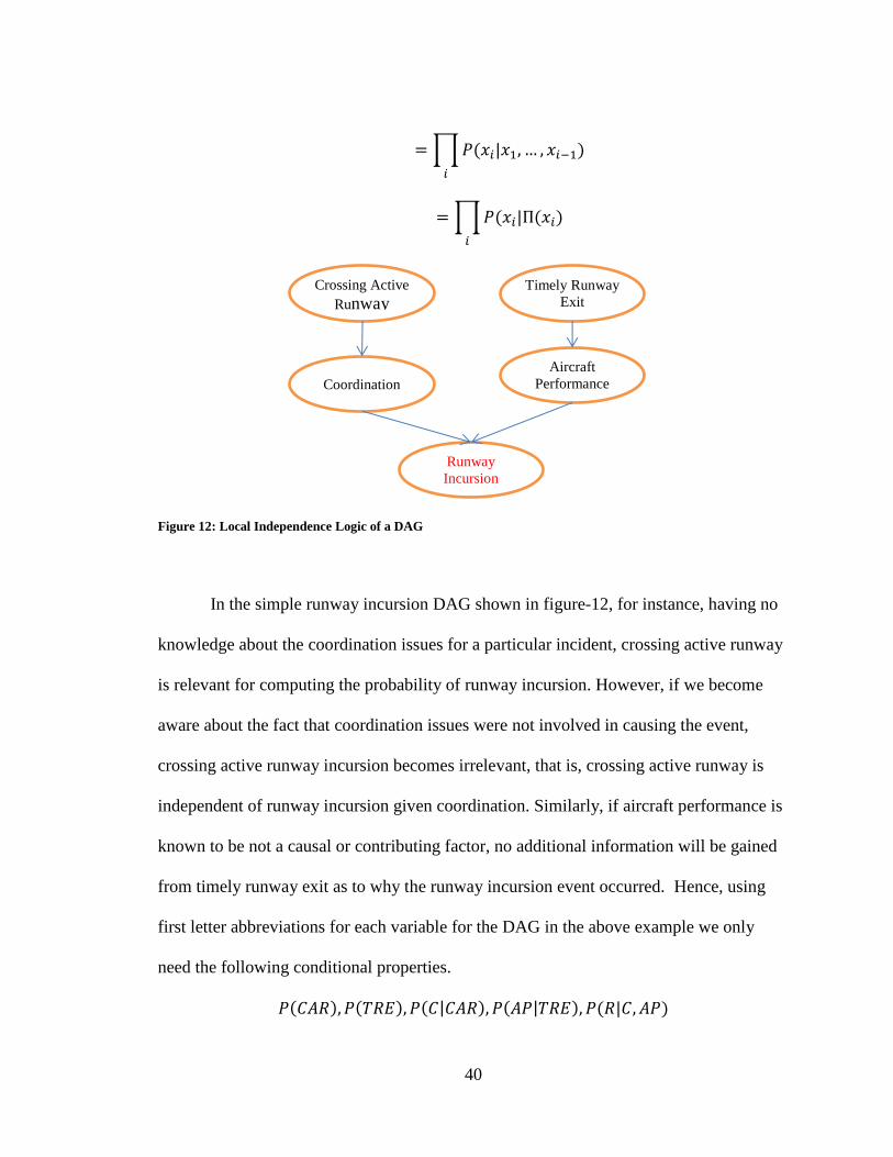
40
∏ ( | )
∏ ( | ( )
Figure 12: Local Independence Logic of a DAG
In the simple runway incursion DAG shown in figure-12, for instance, having no
knowledge about the coordination issues for a particular incident, crossing active runway
is relevant for computing the probability of runway incursion. However, if we become
aware about the fact that coordination issues were not involved in causing the event,
crossing active runway incursion becomes irrelevant, that is, crossing active runway is
independent of runway incursion given coordination. Similarly, if aircraft performance is
known to be not a causal or contributing factor, no additional information will be gained
from timely runway exit as to why the runway incursion event occurred. Hence, using
first letter abbreviations for each variable for the DAG in the above example we only
need the following conditional properties.
( ) ( ) ( | ) ( | ) ( | )
Crossing Active
Runway Timely Runway
Exit
Coordination Aircraft
Performance
Runway
Incursion
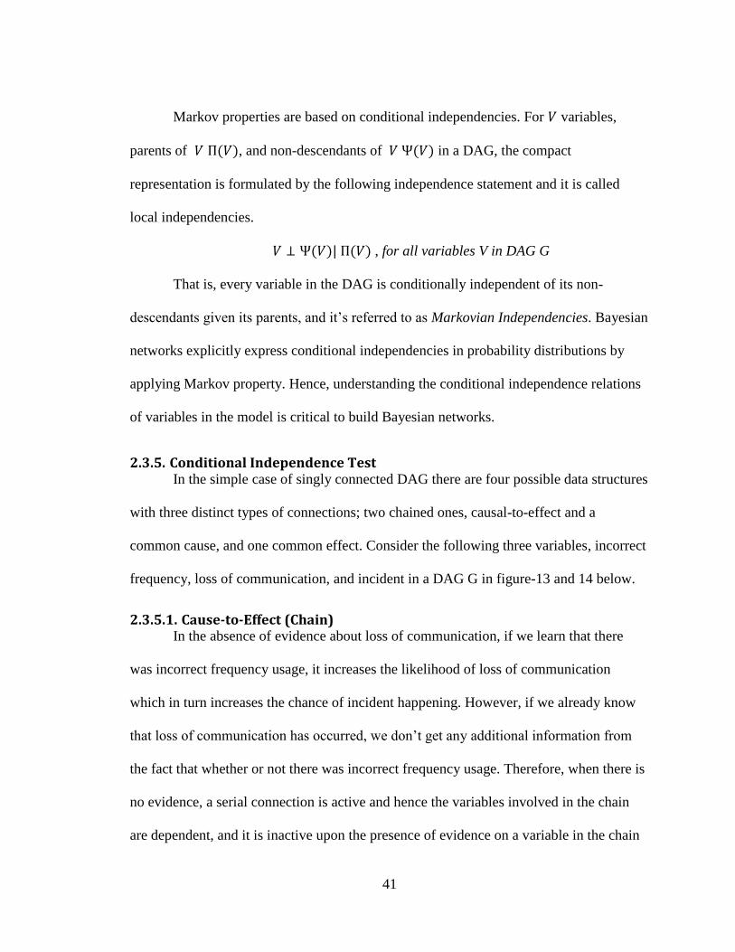
41
Markov properties are based on conditional independencies. For variables,
parents of ( ), and non-descendants of ( ) in a DAG, the compact
representation is formulated by the following independence statement and it is called
local independencies.
( )| ( ) , for all variables V in DAG G
That is, every variable in the DAG is conditionally independent of its non-
descendants given its parents, and it’s referred to as Markovian Independencies. Bayesian
networks explicitly express conditional independencies in probability distributions by
applying Markov property. Hence, understanding the conditional independence relations
of variables in the model is critical to build Bayesian networks.
2.3.5. Conditional Independence Test In the simple case of singly connected DAG there are four possible data structures
with three distinct types of connections; two chained ones, causal-to-effect and a
common cause, and one common effect. Consider the following three variables, incorrect
frequency, loss of communication, and incident in a DAG G in figure-13 and 14 below.
2.3.5.1. Cause-to-Effect (Chain) In the absence of evidence about loss of communication, if we learn that there
was incorrect frequency usage, it increases the likelihood of loss of communication
which in turn increases the chance of incident happening. However, if we already know
that loss of communication has occurred, we don’t get any additional information from
the fact that whether or not there was incorrect frequency usage. Therefore, when there is
no evidence, a serial connection is active and hence the variables involved in the chain
are dependent, and it is inactive upon the presence of evidence on a variable in the chain
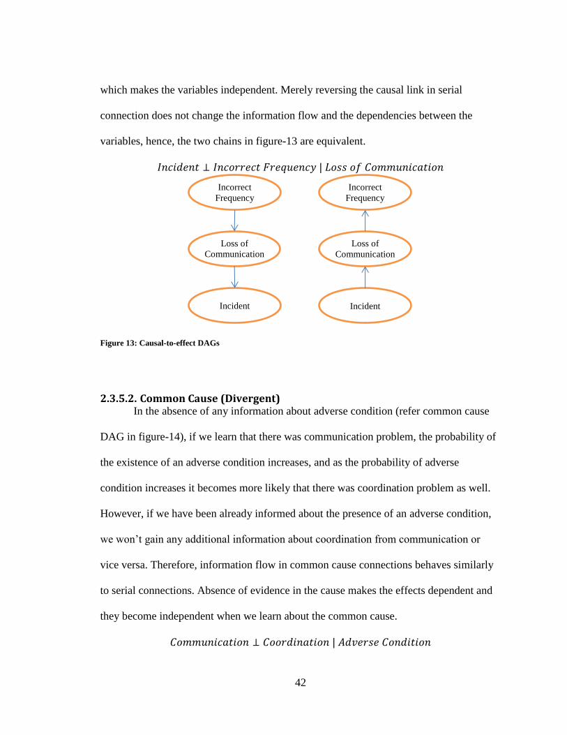
42
which makes the variables independent. Merely reversing the causal link in serial
connection does not change the information flow and the dependencies between the
variables, hence, the two chains in figure-13 are equivalent.
|
Figure 13: Causal-to-effect DAGs
2.3.5.2. Common Cause (Divergent) In the absence of any information about adverse condition (refer common cause
DAG in figure-14), if we learn that there was communication problem, the probability of
the existence of an adverse condition increases, and as the probability of adverse
condition increases it becomes more likely that there was coordination problem as well.
However, if we have been already informed about the presence of an adverse condition,
we won’t gain any additional information about coordination from communication or
vice versa. Therefore, information flow in common cause connections behaves similarly
to serial connections. Absence of evidence in the cause makes the effects dependent and
they become independent when we learn about the common cause.
|
Incorrect
Frequency
Loss of
Communication
Incident
Incorrect
Frequency
Loss of
Communication
Incident
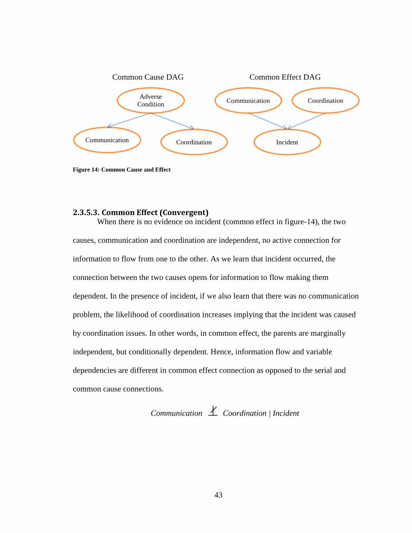
43
Figure 14: Common Cause and Effect
2.3.5.3. Common Effect (Convergent) When there is no evidence on incident (common effect in figure-14), the two
causes, communication and coordination are independent, no active connection for
information to flow from one to the other. As we learn that incident occurred, the
connection between the two causes opens for information to flow making them
dependent. In the presence of incident, if we also learn that there was no communication
problem, the likelihood of coordination increases implying that the incident was caused
by coordination issues. In other words, in common effect, the parents are marginally
independent, but conditionally dependent. Hence, information flow and variable
dependencies are different in common effect connection as opposed to the serial and
common cause connections.
Common Effect DAG
Adverse
Condition
Communication Coordination
Communication Coordination
Incident
Common Cause DAG
Communication Coordination | Incident
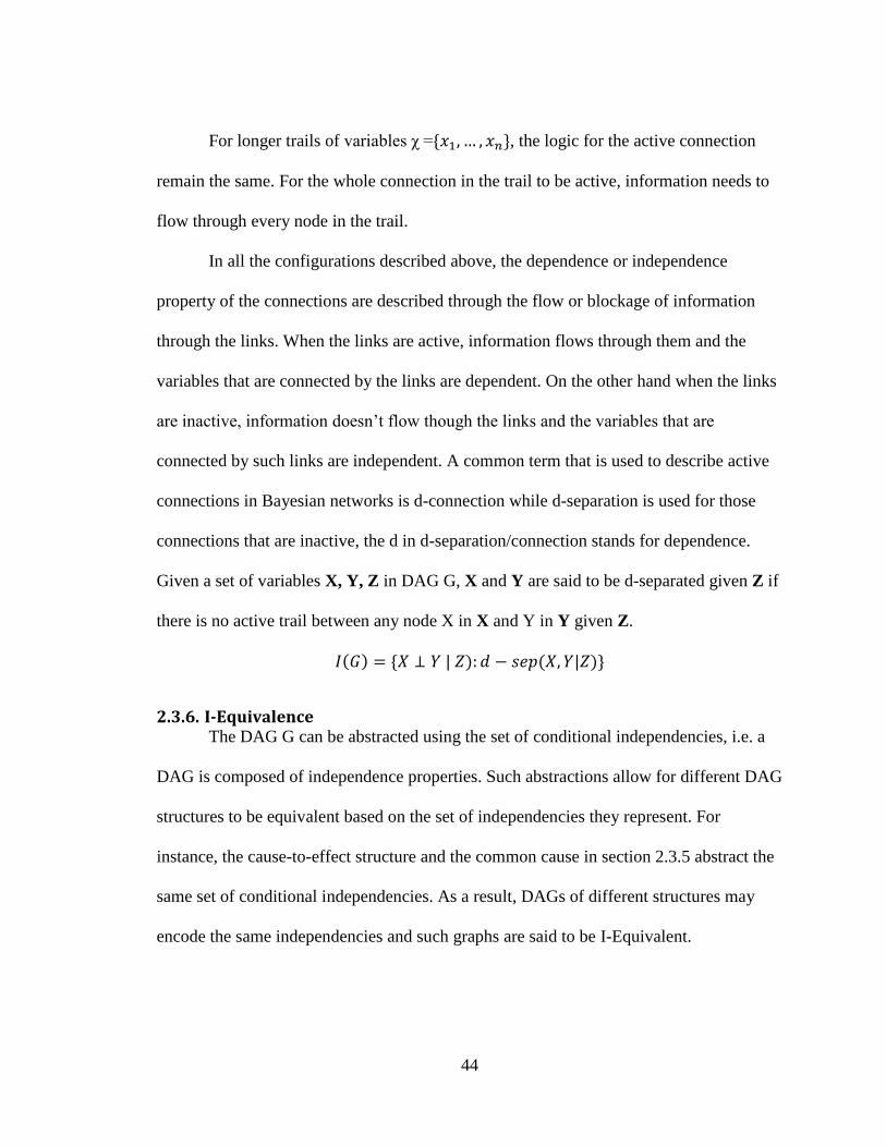
44
For longer trails of variables χ = , the logic for the active connection
remain the same. For the whole connection in the trail to be active, information needs to
flow through every node in the trail.
In all the configurations described above, the dependence or independence
property of the connections are described through the flow or blockage of information
through the links. When the links are active, information flows through them and the
variables that are connected by the links are dependent. On the other hand when the links
are inactive, information doesn’t flow though the links and the variables that are
connected by such links are independent. A common term that is used to describe active
connections in Bayesian networks is d-connection while d-separation is used for those
connections that are inactive, the d in d-separation/connection stands for dependence.
Given a set of variables X, Y, Z in DAG G, X and Y are said to be d-separated given Z if
there is no active trail between any node X in X and Y in Y given Z.
( ) | ) ( | )
2.3.6. I-Equivalence The DAG G can be abstracted using the set of conditional independencies, i.e. a
DAG is composed of independence properties. Such abstractions allow for different DAG
structures to be equivalent based on the set of independencies they represent. For
instance, the cause-to-effect structure and the common cause in section 2.3.5 abstract the
same set of conditional independencies. As a result, DAGs of different structures may
encode the same independencies and such graphs are said to be I-Equivalent.

45
2.3.7. Learning Bayesian Networks Bayesian networks that model real world problems usually involve a fairly large
number of variables and as a result without applying some level of automation it can be
very difficult to construct such models. In fact one of the main challenges to model
problems using Bayesian networks is the difficulty of eliciting knowledge from experts to
determine the structure and probability distributions of the network unique to the domain.
For years researchers have been working on algorithms to learn Bayesian networks from
data to assist the knowledge gathered from experts. In cases where it is difficult to elicit
knowledge from domain experts, data alone may be used for building reasoning models.
Primarily, learning Bayesian networks involve two components; the causal structure of
the network, the DAG, to discover the dependencies in the model, and learning the
parameters of the structure, the CPDs. There are various types of algorithms to do both
but it is beyond the scope of this research to cover them in detail. Once the DAG and
CPD of the networks are learned, the model can be used for purposes of classification,
diagnosis/causation, or prediction. Like many other machine learning algorithms,
learning Bayesian networks from data can be done from samples; a training set is used to
train the model and testing set is used for validating the learned model.
2.3.7.1. Parameter Learning (Estimation) After the structure (DAG) has been created, either by eliciting knowledge from
experts or using algorithms from data, a Bayesian network needs to be parameterized.
Parameterization involves specifying conditional probability distributions on each
variable in the network, which also can be done either through assistance from domain
experts or learning from data or a combination of the two. The two main approaches of

46
parameter learning from data are maximum likelihood estimation and Bayesian parameter
estimation. Below is a brief discussion of both approaches for complete data; the learning
algorithms for incomplete data are more involved—Expectation Maximization and
Gradient Descent are few of the popular algorithms for learning from data with missing
values.
2.3.7.2. Parameter Learning using ML Estimation Maximum likelihood estimation (MLE) is based on the likelihood principle which
favors estimators that maximize the probability of observing the dataset, which is
assumed to be independent and identically distributed (IID). Assume a binomial model of
a single variable, for instance, Aircraft Performance in one of this project’s networks,
which can take the binary states Factor (T) and Not-Factor (F). Also assume that the
probability of the Aircraft Performance being a Factor to an incident is controlled by a
constant but unknown parameter [ ], therefore, the probability that it is Not-Factor
is .
Now if we have a sample of cases of 5 incident reports in which 2 of the incidents
were caused by Aircraft Performance, then the probability of this set of sequences is
( ) ( )( )( ) ( )
The probability depends on the value of hence it is a function of . Therefore,
the likelihood function is
( ) ( ) ( )
For a binary variable if we have C1 number of cases from state 1 and C2 cases
from state 2 of a dataset D, the likelihood function is
47
( ) ( )
It is easier to work with the log-likelihood since the products are replaced with
summations and the two functions are monotonically related.
( ) ( ) ( )
Solving for and denoting by for estimate, by differentiating the log-likelihood
and setting the derivative to 0,
In our example above, the probability of Aircraft Performance being a factor is
( )
In general the likelihood function of a network DAG G and the set of all
parameter estimates for G and ( ) be the probability distribution induced by structure
G and estimates ,
( ) ∏ ( )
And the ML estimator is
( )
2.3.7.3. Parameter Learning using Bayesian Estimation Bayesian estimator is based on conditioning a prior distribution P on parameter
[ ] and using the given dataset as evidence to compute the posterior distribution to
estimate the parameter; note that is treated as a random variable in this setting. For the
48
binomial model we considered above for the MLE, the joint distribution of the dataset
and is,
( ) ( | ) ( )
= ( ) ( )
In general for incidents with evidence of only of them caused by Aircraft
Performance,
( | ) ( ) ( )
This is a product of the likelihood and the prior distribution. The posterior
distribution is,
( | ) ( | ) ( )
Where ( )⁄
The posterior is proportional to the product of the likelihood and the prior, and the
denominator is a normalizing factor to make the posterior a proper density function. The
above equation needs a prior distribution over although the specific type of the
distribution is less relevant. However, one of the commonly used families of distributions
for prior belief is beta distribution. A beta distribution is parameterized by two
hyperparameters , both of which are positive reals.
( )
( | ) ( )
( )
( ) ( ) ( ) ∫
49
In our binomial example may represent Aircraft Performance being a factor to
an incident and not a factor.
The expected value of the beta distribution is,
( ( )) ∫ ( | )
In our example of Aircraft Performance factors in incidents,
( | ) ( ) ( )
This is another beta distribution with different parameter values,
( )
Therefore, both the prior and the posterior are in the same family of beta
distribution and such distributions are known as conjugate family of distribution. The
convenience of conjugacy is one of the reasons for using beta distribution as a prior in
Bayesian parameter estimation.
If we assign a ( ) prior in our example (figure-15), and with the
observation of 2 Aircraft Performance factors in 5 observations,
( | ) ( ( ) ( )
The expectation,
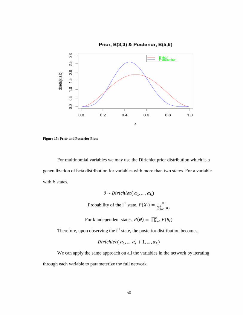
50
Figure 15: Prior and Posterior Plots
For multinomial variables we may use the Dirichlet prior distribution which is a
generalization of beta distribution for variables with more than two states. For a variable
with states,
( )
Probability of the ith
state, ( )
∑
For k independent states, ( ) ∏ ( )
Therefore, upon observing the ith
state, the posterior distribution becomes,
( )
We can apply the same approach on all the variables in the network by iterating
through each variable to parameterize the full network.

51
2.3.7.4. Structure Learning In the network parameterization discussion above, the assumption we made is that
the structure is given. However, in any real world problem the structure of the network
needs to be learned from data or elicited from domain experts. It is important to
remember that due to potential I-equivalence among various network structures for the
same domain, the DAG may not be unique. In general, learning network structure is
much harder than learning network parameters; it is problem, and as a result
sometimes heuristic methods are used along with algorithm-driven learning.
Primarily there are two approaches for learning Bayesian structure; constraint-
based learning and score-based learning. In addition, model averaging methods which
generate an ensemble of possible structures can be considered as a third approach.
Constraint-based learning is based on discovering independencies between variables in
the data and model the structure to reflect these independencies. Score-based methods on
the other hand are used by scoring all the potential structures in the domain and selecting
the model with the highest score. Similar to parameter learning, score-based structure
learning may be learnt by likelihood principle or Bayesian approach.
For the models learnt in this dissertation part of the structure is built based on the
information embedded in the dataset, that is, we know the causal factors are correlated to
the target events, hence we link them in the network. Also, since the hierarchical
abstraction is only for the purpose of simplifying the network structure, there is always a
link between the parent and its children in the hierarchy. However, the relationships
between causal factors are unknown, which requires “partial” structure learning. I use
Tree-Augmented Naïve (TAN) structure learning to discover associations between any

52
pair of causal factors given the structure learned using the top causal factors identified for
each event. The methodologies chapter provides the description about TAN structure
learning and the justification for applying it in this setting.
2.3.7.5. Likelihood Scoring The objective in likelihood scoring is to maximize the likelihood function, i.e. to
find a structure that makes the observed data as probable as possible. For k possible
structures , the likelihood score (LS) for the G is given by,
( ) ( )
Where ( ) is the log-likelihood function as defined above in the
parameter learning section and is the maximum likelihood parameter for .
ML ignores a conditional independence unless it holds exactly in the empirical
distribution, which is unlikely in most samples, and hence it tends to create fully
connected networks which causes over fitting by mirroring the training dataset.
2.3.7.6. Bayesian Scoring Similar to Bayesian parameter learning, we place a prior distribution over the
structure about which we have uncertainty and its parameters. For k possible
structures , the posterior probability of the G is given by,
( | ) ( | ) ( )
( ) ( )
The ( ) is a normalizing factor which doesn’t contribute in differentiating
structures and the prior ( ) is irrelevant compared to the marginal distribution ( | ).
Therefore, the Bayesian Score (BS) in log form to avoid numeric underflow for large
networks is given by,
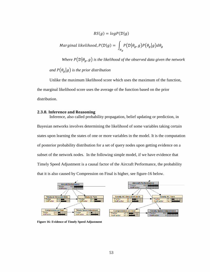
53
( ) ( | )
( | ) ∫ ( | ) ( | )
Where ( | ) is the likelihood of the observed data given the network
and ( | ) is the prior distribution
Unlike the maximum likelihood score which uses the maximum of the function,
the marginal likelihood score uses the average of the function based on the prior
distribution.
2.3.8. Inference and Reasoning Inference, also called probability propagation, belief updating or prediction, in
Bayesian networks involves determining the likelihood of some variables taking certain
states upon learning the states of one or more variables in the model. It is the computation
of posterior probability distribution for a set of query nodes upon getting evidence on a
subset of the network nodes. In the following simple model, if we have evidence that
Timely Speed Adjustment is a causal factor of the Aircraft Performance, the probability
that it is also caused by Compression on Final is higher, see figure-16 below.
Figure 16: Evidence of Timely Speed Adjustment
54
Bayesian inference is primarily based on Bayesian philosophy, which lies in the
interpretation of Bayes’ theorem to propagate flow of information through the network.
( | ) ( | ) ( )
( )
This is a simple theorem of probability that can easily be proved using definition
of conditional probability. It implies that the probability of event conditioned upon
evidence is the product of the likelihood ( | ) and the probability of before any
evidence ( ), which is called the prior, normalized by ( ) so that the total conditional
probabilities sum to 1. It is basically adjusting of one’s belief given new evidence, and it
is usually known as posterior probability. The evidence can come as hard evidence, with
100% certainty in the given state, or soft/likelihood evidence with probability of less than
100%.
There are two major inference algorithms—exact and approximate, and the type
of the network and the complexity of the model dictate the kind of inference algorithm
applied to the problem. Iterated application of Bayes' theorem may well suffice for a
simply chained network, while networks with multiple paths to nodes may require more
sophisticated algorithms. Similarly, exact inference algorithms may be available for
simpler networks, but such algorithms may involve expensive computations in which
case approximate algorithms can give sufficiently satisfactory solutions. In this research I
use Netica’s software Application Programming Interface (API), which uses junction tree
algorithm to propagate evidences by message passing. A message passing algorithm
(Pearl, 1988) is an efficient inference algorithm which exploits local independencies to
pass information between neighbors recursively.

55
2.3.9. Decision Network Standard Bayesian networks don’t provide any specific recommendations to alter,
minimize, or optimize the interrelationships among the causal and effect variables in the
model. Moreover, classical probabilistic queries don’t depend on the causality of the
network so long as they encode the correct distribution and hence it is not always
predictable how intervening influences the causality in the network. However,
intervening or taking actions on causal models can lead to a different outcome of the
distribution in the network thereby influencing the natural course of events. By assigning
a value or utility to different situations, we can rank each possible outcome and influence
the result according to the rank assigned.
In this research I will incorporate a simple cost-based utility function in the
runway incursion event causal model to demonstrate the value of converting ordinary
probabilistic model to a decision network. Such a model suggests specific actions to be
taken in order to maximize the utility, which is to minimize the occurrence of causal
factors according to their frequency in causing incidents and their severity. For instance,
by addressing the causal factors that lead to major incidents, we can lessen the effects of
the problems in causing potential accidents. Utility functions that are involved in most
models incorporate monetary values as taking any action usually incurs cost. However,
due to the scope of this research, I will limit the financial aspect of the cost associated
with taking a particular action such as fixing any specific problem in this domain.
In figure 17, the control variables are the actions that need to be taken in order to
reduce the likelihood of the causal factors that eventually lead to the underlying event. In
real world problems the actions we take are not usually perfect, they don’t entirely
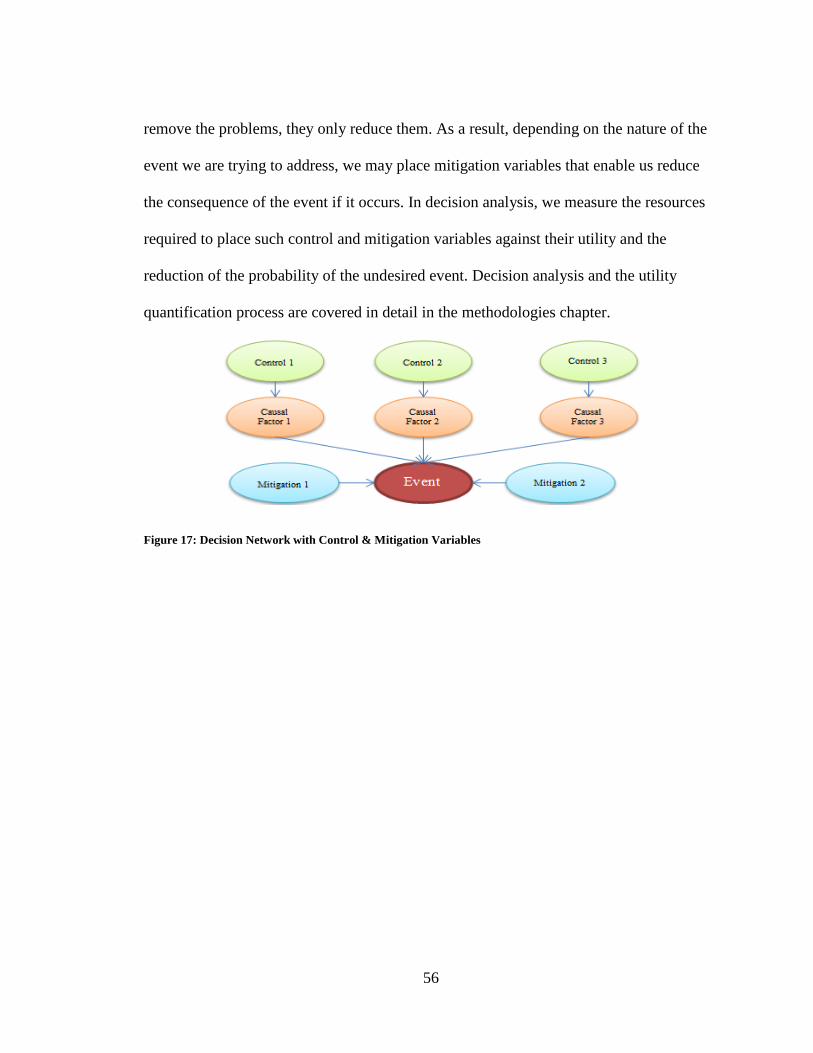
56
remove the problems, they only reduce them. As a result, depending on the nature of the
event we are trying to address, we may place mitigation variables that enable us reduce
the consequence of the event if it occurs. In decision analysis, we measure the resources
required to place such control and mitigation variables against their utility and the
reduction of the probability of the undesired event. Decision analysis and the utility
quantification process are covered in detail in the methodologies chapter.
Figure 17: Decision Network with Control & Mitigation Variables
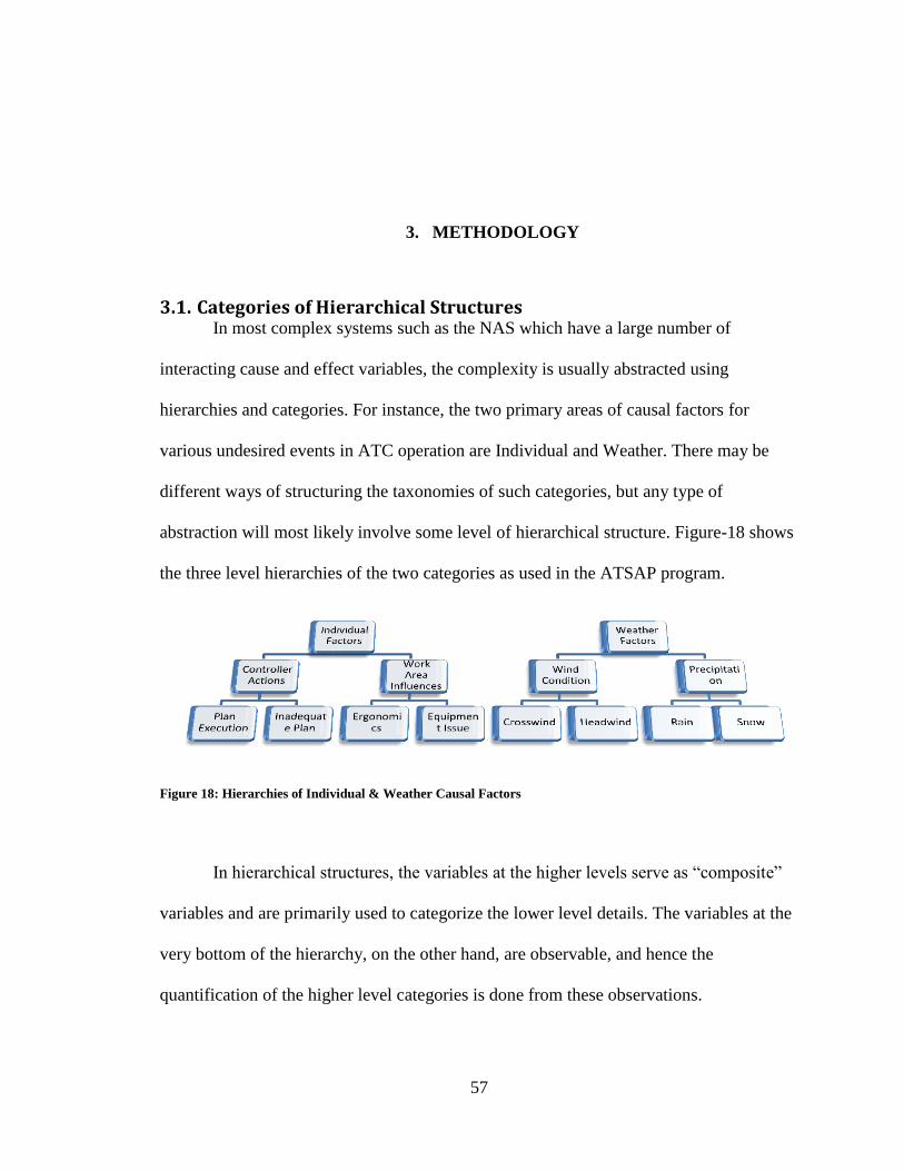
57
3. METHODOLOGY
3.1. Categories of Hierarchical Structures In most complex systems such as the NAS which have a large number of
interacting cause and effect variables, the complexity is usually abstracted using
hierarchies and categories. For instance, the two primary areas of causal factors for
various undesired events in ATC operation are Individual and Weather. There may be
different ways of structuring the taxonomies of such categories, but any type of
abstraction will most likely involve some level of hierarchical structure. Figure-18 shows
the three level hierarchies of the two categories as used in the ATSAP program.
Figure 18: Hierarchies of Individual & Weather Causal Factors
In hierarchical structures, the variables at the higher levels serve as “composite”
variables and are primarily used to categorize the lower level details. The variables at the
very bottom of the hierarchy, on the other hand, are observable, and hence the
quantification of the higher level categories is done from these observations.
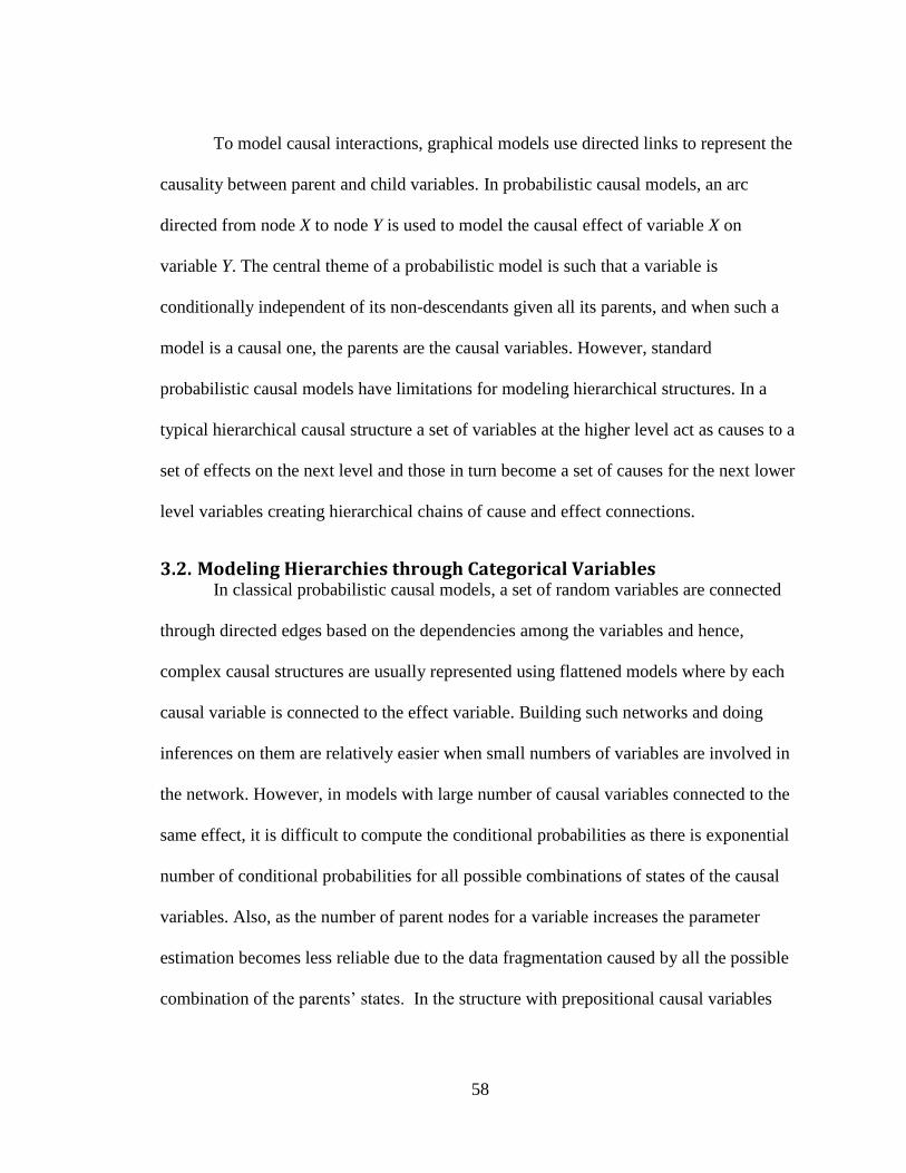
58
To model causal interactions, graphical models use directed links to represent the
causality between parent and child variables. In probabilistic causal models, an arc
directed from node X to node Y is used to model the causal effect of variable X on
variable Y. The central theme of a probabilistic model is such that a variable is
conditionally independent of its non-descendants given all its parents, and when such a
model is a causal one, the parents are the causal variables. However, standard
probabilistic causal models have limitations for modeling hierarchical structures. In a
typical hierarchical causal structure a set of variables at the higher level act as causes to a
set of effects on the next level and those in turn become a set of causes for the next lower
level variables creating hierarchical chains of cause and effect connections.
3.2. Modeling Hierarchies through Categorical Variables In classical probabilistic causal models, a set of random variables are connected
through directed edges based on the dependencies among the variables and hence,
complex causal structures are usually represented using flattened models where by each
causal variable is connected to the effect variable. Building such networks and doing
inferences on them are relatively easier when small numbers of variables are involved in
the network. However, in models with large number of causal variables connected to the
same effect, it is difficult to compute the conditional probabilities as there is exponential
number of conditional probabilities for all possible combinations of states of the causal
variables. Also, as the number of parent nodes for a variable increases the parameter
estimation becomes less reliable due to the data fragmentation caused by all the possible
combination of the parents’ states. In the structure with prepositional causal variables
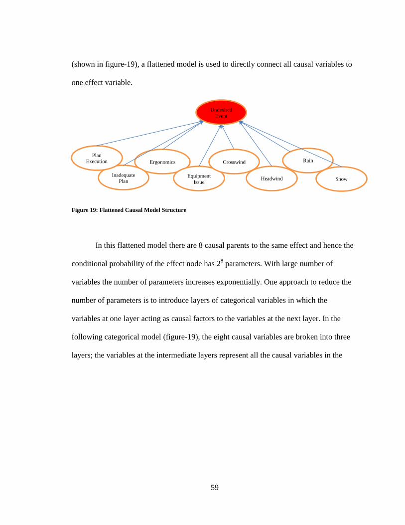
59
(shown in figure-19), a flattened model is used to directly connect all causal variables to
one effect variable.
Figure 19: Flattened Causal Model Structure
In this flattened model there are 8 causal parents to the same effect and hence the
conditional probability of the effect node has 28 parameters. With large number of
variables the number of parameters increases exponentially. One approach to reduce the
number of parameters is to introduce layers of categorical variables in which the
variables at one layer acting as causal factors to the variables at the next layer. In the
following categorical model (figure-19), the eight causal variables are broken into three
layers; the variables at the intermediate layers represent all the causal variables in the
Ergonomics
Inadequate Plan
Equipment
Issue
Plan Execution Rain Crosswind
Headwind Snow
Undesired
Event
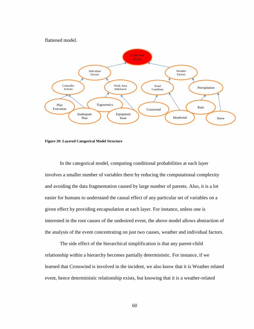
60
flattened model.
Figure 20: Layered Categorical Model Structure
In the categorical model, computing conditional probabilities at each layer
involves a smaller number of variables there by reducing the computational complexity
and avoiding the data fragmentation caused by large number of parents. Also, it is a lot
easier for humans to understand the causal effect of any particular set of variables on a
given effect by providing encapsulation at each layer. For instance, unless one is
interested in the root causes of the undesired event, the above model allows abstraction of
the analysis of the event concentrating on just two causes, weather and individual factors.
The side effect of the hierarchical simplification is that any parent-child
relationship within a hierarchy becomes partially deterministic. For instance, if we
learned that Crosswind is involved in the incident, we also know that it is Weather related
event, hence deterministic relationship exists, but knowing that it is a weather-related
Ergonomics
Inadequate
Plan Equipment
Issue
Plan
Execution Rain Crosswind
Headwind Snow
Undesired
Event
Controller
Actions
Work Area
Influences Wind
Condition Precipitation
Weather
Factors Individual
Factors
61
incident doesn’t necessarily mean Crosswind is the lower level causal factor, hence
probabilistic relationship exists. On the other hand, the partially deterministic behavior
can be beneficial to further simplify the reasoning process upon learning evidences. For
instance, in the hierarchical model above, if we learned that weather problem was not
involved in causing or contributing to the undesired event in any way, we can provide
negative evidence on the Weather variable alone and effectively remove all the nodes that
are sub categories of the Weather hierarchy making the inference a lot simpler.
In ATSAP ATC taxonomy, there are more than 300 causal factors contributing to
21 undesired event types. The event classification has three high level categories and
each category contains the specific undesired event.
Figure 21: Hierarchies of Undesired Event Types in ATSAP
Similarly, there are 15 high level categories of causal factors with sub categories
ranging from two to four levels. By directly representing the hierarchical structure of the
domain using categorical variables, a level of simplification is achieved in the
probabilistic causal model. The following structure is the output of an automation
program and represents the full hierarchical structure of the events and causal factors. All
the connections are done from one hierarchy to the next which significantly reduces the
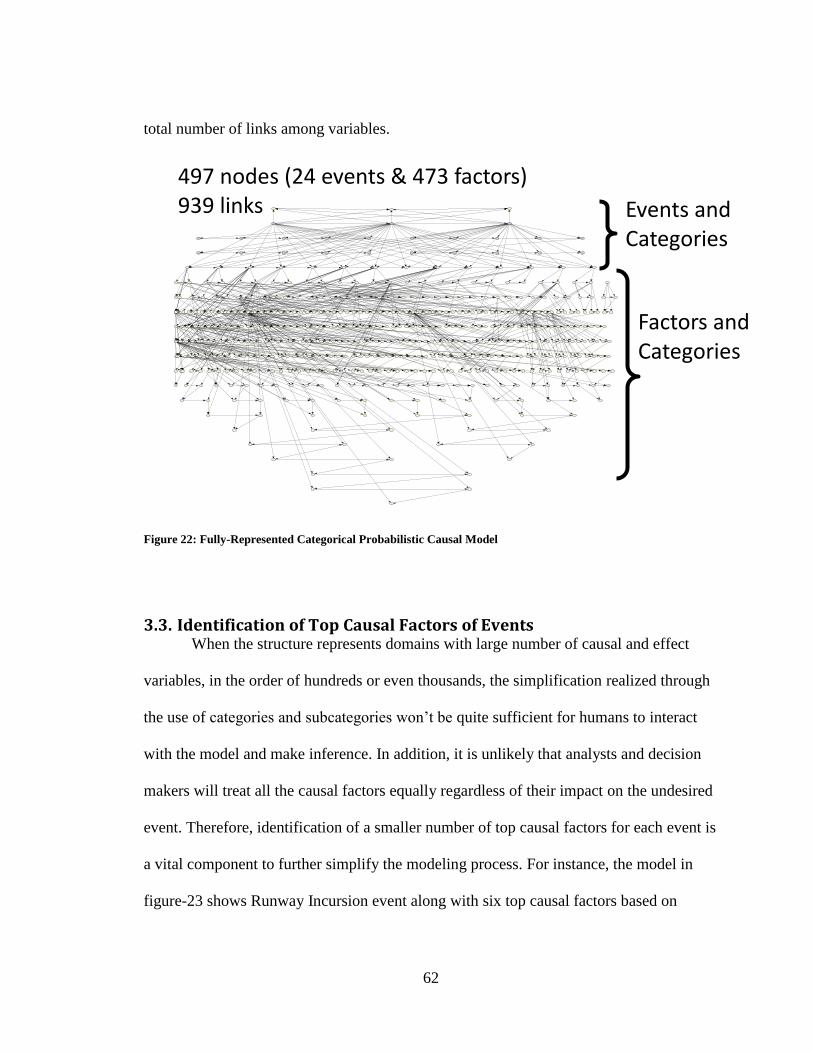
62
total number of links among variables.
Figure 22: Fully-Represented Categorical Probabilistic Causal Model
3.3. Identification of Top Causal Factors of Events When the structure represents domains with large number of causal and effect
variables, in the order of hundreds or even thousands, the simplification realized through
the use of categories and subcategories won’t be quite sufficient for humans to interact
with the model and make inference. In addition, it is unlikely that analysts and decision
makers will treat all the causal factors equally regardless of their impact on the undesired
event. Therefore, identification of a smaller number of top causal factors for each event is
a vital component to further simplify the modeling process. For instance, the model in
figure-23 shows Runway Incursion event along with six top causal factors based on
497 nodes (24 events & 473 factors)
939 links Events and Categories
Factors and Categories
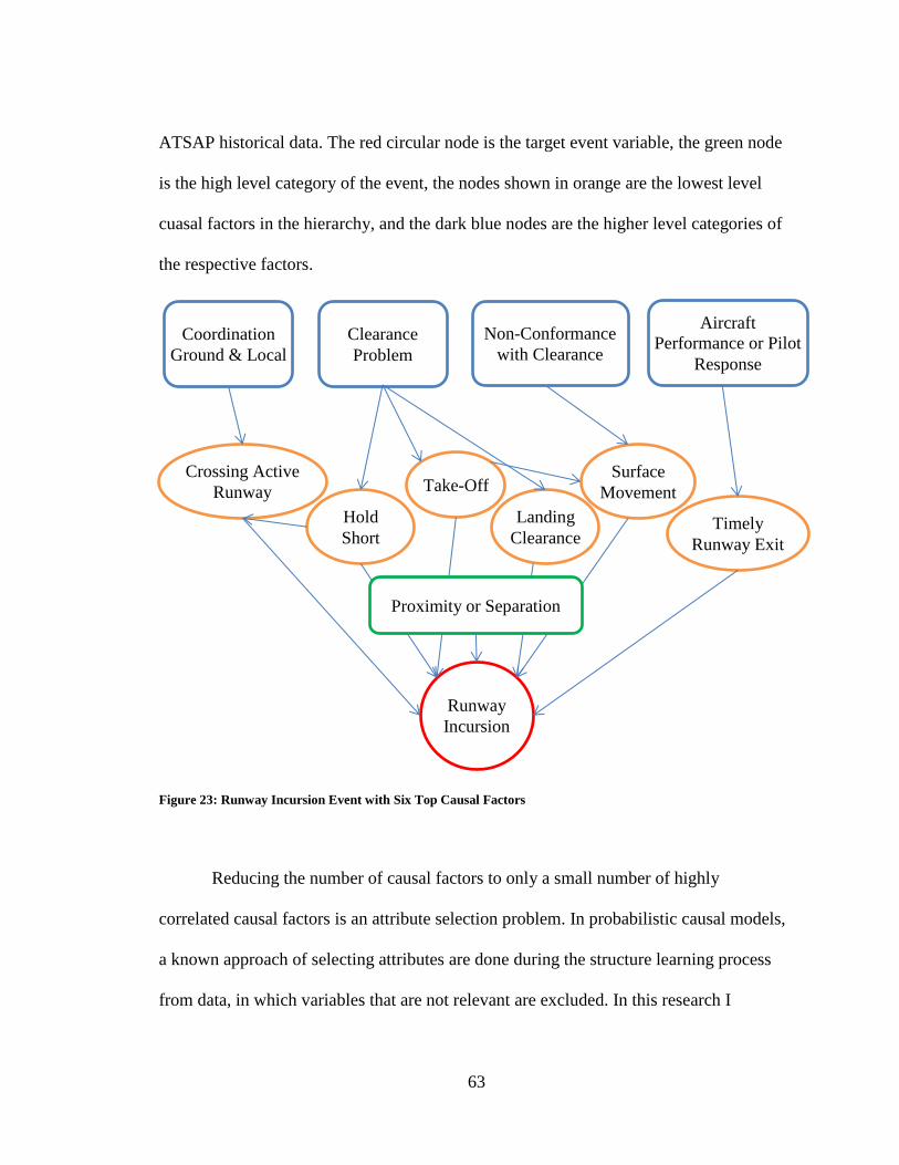
63
ATSAP historical data. The red circular node is the target event variable, the green node
is the high level category of the event, the nodes shown in orange are the lowest level
cuasal factors in the hierarchy, and the dark blue nodes are the higher level categories of
the respective factors.
Figure 23: Runway Incursion Event with Six Top Causal Factors
Reducing the number of causal factors to only a small number of highly
correlated causal factors is an attribute selection problem. In probabilistic causal models,
a known approach of selecting attributes are done during the structure learning process
from data, in which variables that are not relevant are excluded. In this research I
Runway
Incursion
Surface
Movement Take-Off Crossing Active
Runway
Landing
Clearance
Hold
Short Timely
Runway Exit
Clearance
Problem
Non-Conformance
with Clearance
Aircraft
Performance or Pilot
Response
Coordination
Ground & Local
Proximity or Separation
64
introduce an attribute selection approach based on sensitivity analysis and performance
measure of the probabilistic model.
3.3.1. Sensitivity Analysis of Bayesian Networks Sensitivity analysis is primarily used to test the robustness of a probabilistic
model. It is a mechanism to measure the impact of one or more variables on a target
variable in probabilistic graphical models. Sensitivity analysis is primarily used to check
the validity of probabilistic models that are built through the solicitation of expert
opinions. It serves as a tool to correct local probabilistic distributions when the impact of
a set of variables on the target variable is out of expected ranges, excessively high or low
that cannot be explained within the context of the given model. It can also be used to
measure changes on the query variables in order to enforce certain constraints, such as a
pre-specified level or bounds of posterior output on the target variable.
For instance, if one builds a probabilistic model for runway incursion along with
its top causal factors with the help of expert judgment, sensitivity analysis can be
performed to measure the change of the probability that occurs on the runway incursion
event when we provide evidence on some of the causal factors. If the change is deemed
excessive by the expert, then local probability distributions of the affected causal factors
may need to be modified to correct the discrepancy. On the other hand, if the parameter
changes on the causal factors are found to be inadequate, then the network structure may
need to change through the addition or removal of some causal factor nodes.
65
3.3.2. Factor Selection using Performance Measure The identification of top significant causal factors for a given event is a type of
feature selection problem. With a large number of causal factors the accuracy of
classifying events may increase at the expense of complexity. However, it may be
preferable to only include a smaller number of causal factors with an acceptable level of
accuracy thereby reducing the complexity of the model.
In this research I introduce a selection criterion that follows a two-step process. In
the first step, the impact of each causal factor is measured using a posterior calculation
and the relevant causal factors are ranked as described in the impact of factors section
below. In the second step, multiple networks are created iteratively by incorporating
causal factors according to their rank. The steps of the model simplification process are,
1. The impact of each causal factor for the target event is calculated as the difference
of prior and posterior probabilities for ranking
2. A network with the given event as a target and a causal factor with the highest
rank is created
3. The network parameters are learned using the training dataset
4. The performance of the network is measured using the test dataset and the
classification accuracy is calculated using Brier score (section 3.3.4)
The process continues, and more high-rank causal factors are added, the network
retrained, and the reduction of the Brier score of subsequent iterations is calculated. The
stopping criteria for not adding more causal factors is such that the reduction of the Brier
score on the test dataset is smaller than the immediate previous iteration. The final
network is comprised of the top causal factors linked to the target event variable along
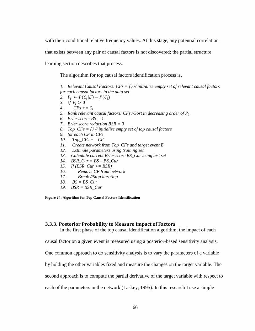
66
with their conditional relative frequency values. At this stage, any potential correlation
that exists between any pair of causal factors is not discovered; the partial structure
learning section describes that process.
The algorithm for top causal factors identification process is,
1. Relevant Causal Factors: CFs = {} // initialize empty set of relevant causal factors
for each causal factors in the data set
2. ( | ) ( )
3.
4. CFs +=
5. Rank relevant causal factors: CFs //Sort in decreasing order of
6. Brier score: BS = 1
7. Brier score reduction BSR = 0
8. Top_CFs = {} // initialize empty set of top causal factors
9. for each CF in CFs
10. Top_CFs += CF
11. Create network from Top_CFs and target event E
12. Estimate parameters using training set
13. Calculate current Brier score BS_Cur using test set
14. BSR_Cur = BS – BS_Cur
15. If (BSR_Cur <= BSR)
16. Remove CF from network
17. Break //Stop iterating
18. BS = BS_Cur
19. BSR = BSR_Cur
Figure 24: Algorithm for Top Causal Factors Identification
3.3.3. Posterior Probability to Measure Impact of Factors In the first phase of the top causal identification algorithm, the impact of each
causal factor on a given event is measured using a posterior-based sensitivity analysis.
One common approach to do sensitivity analysis is to vary the parameters of a variable
by holding the other variables fixed and measure the changes on the target variable. The
second approach is to compute the partial derivative of the target variable with respect to
each of the parameters in the network (Laskey, 1995). In this research I use a simple
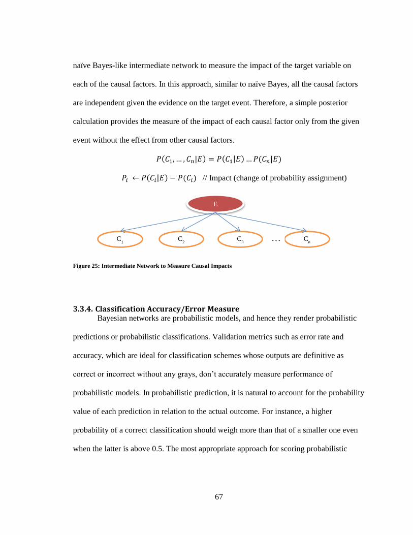
67
naïve Bayes-like intermediate network to measure the impact of the target variable on
each of the causal factors. In this approach, similar to naïve Bayes, all the causal factors
are independent given the evidence on the target event. Therefore, a simple posterior
calculation provides the measure of the impact of each causal factor only from the given
event without the effect from other causal factors.
( | ) ( | ) ( | )
( | ) ( ) // Impact (change of probability assignment)
Figure 25: Intermediate Network to Measure Causal Impacts
3.3.4. Classification Accuracy/Error Measure Bayesian networks are probabilistic models, and hence they render probabilistic
predictions or probabilistic classifications. Validation metrics such as error rate and
accuracy, which are ideal for classification schemes whose outputs are definitive as
correct or incorrect without any grays, don’t accurately measure performance of
probabilistic models. In probabilistic prediction, it is natural to account for the probability
value of each prediction in relation to the actual outcome. For instance, a higher
probability of a correct classification should weigh more than that of a smaller one even
when the latter is above 0.5. The most appropriate approach for scoring probabilistic
E
C1 C
2 C
3 C
n …
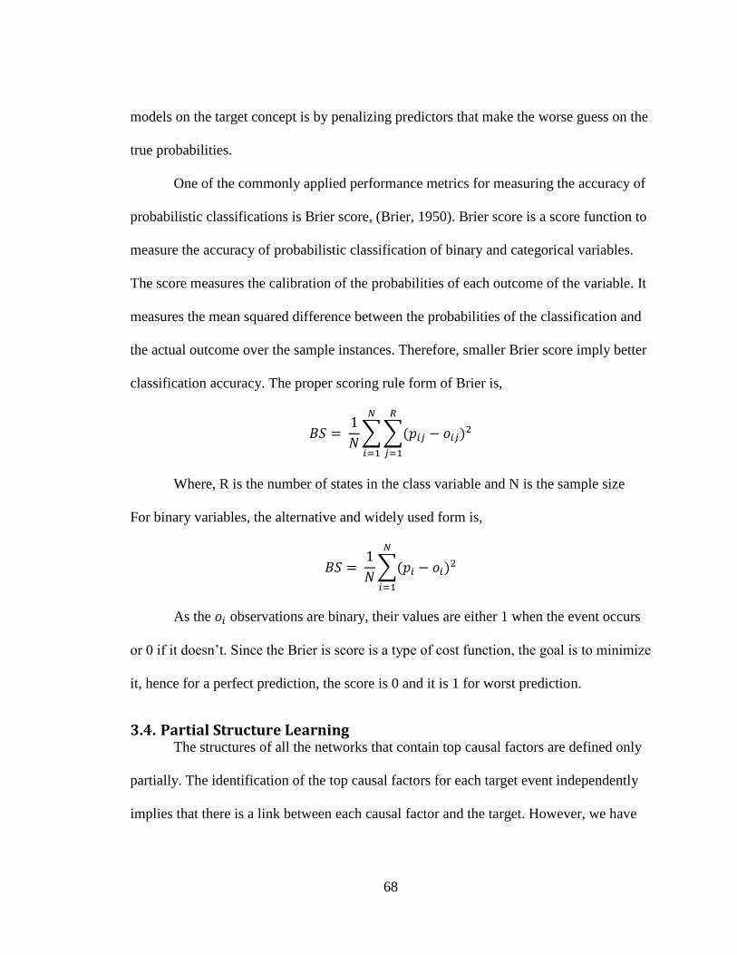
68
models on the target concept is by penalizing predictors that make the worse guess on the
true probabilities.
One of the commonly applied performance metrics for measuring the accuracy of
probabilistic classifications is Brier score, (Brier, 1950). Brier score is a score function to
measure the accuracy of probabilistic classification of binary and categorical variables.
The score measures the calibration of the probabilities of each outcome of the variable. It
measures the mean squared difference between the probabilities of the classification and
the actual outcome over the sample instances. Therefore, smaller Brier score imply better
classification accuracy. The proper scoring rule form of Brier is,
∑∑( )
Where, R is the number of states in the class variable and N is the sample size
For binary variables, the alternative and widely used form is,
∑( )
As the observations are binary, their values are either 1 when the event occurs
or 0 if it doesn’t. Since the Brier is score is a type of cost function, the goal is to minimize
it, hence for a perfect prediction, the score is 0 and it is 1 for worst prediction.
3.4. Partial Structure Learning The structures of all the networks that contain top causal factors are defined only
partially. The identification of the top causal factors for each target event independently
implies that there is a link between each causal factor and the target. However, we have

69
yet to determine the correlations between the top causal factors which can only be
achieved by applying a structure learning scheme. In general, structure learning is a more
challenging problem, particularly when a large number of variables are involved. The
following section describes the type of structure learning used for this problem and some
of the reasoning behind choosing the learning algorithm.
3.4.1. Unsupervised Structure Learning Most structure learning algorithms in use today are in the form of unsupervised
learning, they don’t separate the target variable from the attributes. They learn the
network by trying to identify a set of structures that represent the probability distribution
over the training dataset and take the best one using some kind of ranking (Friedman and
Goldszmidt, 1996). Hence, such algorithms follow a kind of optimization process by
incorporating search techniques, usually heuristic ones, over the space of available
structures and using various scoring function to determine the best structure with respect
to the training data. For most real world problems, the optimization process is intractable
due to the large space of available structures. As a result almost all search and score-
based algorithms apply restrictions to only cover certain classes of structures, for
instance, using sampling, and can learn the “best” structure in polynomial time. One such
heuristic-search algorithm is the K2 algorithm (Cooper and Herskovits, 1992), which
applies certain ordering of the domain variables and each variable can only have a given
maximum number of parents with respect to the ordering.
Search and score-based structure learning methods have theoretical justification in
terms of their asymptotical correctness. Given a large set of independent samples, the

70
learned structure is a close approximation for the probability distribution of the data
generating process. However, in reality they could present a classifier with poor
classification accuracy even though they may have relatively higher scores. Empirical
analyses suggest that score-based structure learning occasionally results in inconsistent
output, i.e. a network with a better score is not necessarily a better classifier (Friedman
and Goldszmidt, 1997). There are multiple factors for the inconsistency of such results,
such as the type of data, sample size, number of variables etc. However, the primary
reason is the type of score function used. In their experiment, Friedman and Goldszmidt
verified that a classifier based on the Minimum Description Language (MDL) score
function performed poorly on many datasets involving more than fifteen variables.
Almost all such learning methods involve feature selection by which they remove
irrelevant variables which is mostly a very useful component of the classification process.
However, occasionally, the feature selection process removes relevant variables which
can have serious consequences in the classification performance.
In this research, the feature selection algorithm is done independently using
algorithms described in previous sections. As a result, using the heuristic search and
score approaches for the purpose of learning the partial structures has negative
consequences. Based on experiments I have conducted using K2 and Hill Climbing to do
the structure learning, both rendered less than optimal results. K2 provided none to very
few correlations between the causal factors and Hill Combing resulted in excessively
complex network on the twenty one event models and a total of eighty top causal factors.
71
3.4.2. Tree-Augmented Naïve (TAN) Bayesian Structure Learning Despite its unrealistic strong independence assumption, naïve Bayes classifier has
shown surprisingly good results in various domains. Naïve Bayes classifier learns the
conditional probability of each attribute given the target variable, and the classification is
done by applying simple Bayes rule; all the attributes are assumed to be independent
given the target which makes it computationally very feasible. It considers all the
attributes as relevant so as to determine the class of the target variable. In the context of
probabilistic networks, attribute relevance is based on the notion of Markov blanket of a
given variable. Markov blanket of a variable includes parents of the variable, its children,
and the parents of its children (Pearl, 1988).
TAN is a structure learning algorithm which extends the naïve Bayes classifier,
and it approximates the interactions between attributes by using a tree structure imposed
on the naïve Bayes structure and is a polynomial time algorithm (Friedman and
Goldszmidt, 1997). Experiments show that TAN performs significantly better on many
dataset compared to C4.5 and naïve Bayes. The performance improvement of TAN in
classifying the target variable is attributed to the fact that it gives special emphasis to the
target variable by enforcing a link between the target variable and each attribute. For
instance, applying the TAN learning scheme in the Runway Incursion network, because
of the augmented edges, there exists a link between Crossing Active Runway and Hold
Short Clearance causal factors signifying that the impact of Crossing Active Runway on
Runway Incursion events is dependent on the influence of Hold Short clearance. Similar
to other unrestricted search algorithms, discovering the set of augmented edges of TAN
learning to determine the best structure is an intractable problem. As proposed by
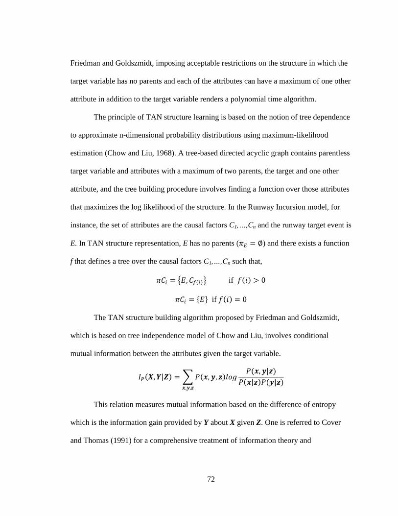
72
Friedman and Goldszmidt, imposing acceptable restrictions on the structure in which the
target variable has no parents and each of the attributes can have a maximum of one other
attribute in addition to the target variable renders a polynomial time algorithm.
The principle of TAN structure learning is based on the notion of tree dependence
to approximate n-dimensional probability distributions using maximum-likelihood
estimation (Chow and Liu, 1968). A tree-based directed acyclic graph contains parentless
target variable and attributes with a maximum of two parents, the target and one other
attribute, and the tree building procedure involves finding a function over those attributes
that maximizes the log likelihood of the structure. In the Runway Incursion model, for
instance, the set of attributes are the causal factors C1,…,Cn and the runway target event is
E. In TAN structure representation, E has no parents ( ) and there exists a function
f that defines a tree over the causal factors C1,…,Cn such that,
{ ( )} if ( )
if ( )
The TAN structure building algorithm proposed by Friedman and Goldszmidt,
which is based on tree independence model of Chow and Liu, involves conditional
mutual information between the attributes given the target variable.
( | ) ∑ ( ) ( | )
( | ) ( | )
This relation measures mutual information based on the difference of entropy
which is the information gain provided by Y about X given Z. One is referred to Cover
and Thomas (1991) for a comprehensive treatment of information theory and
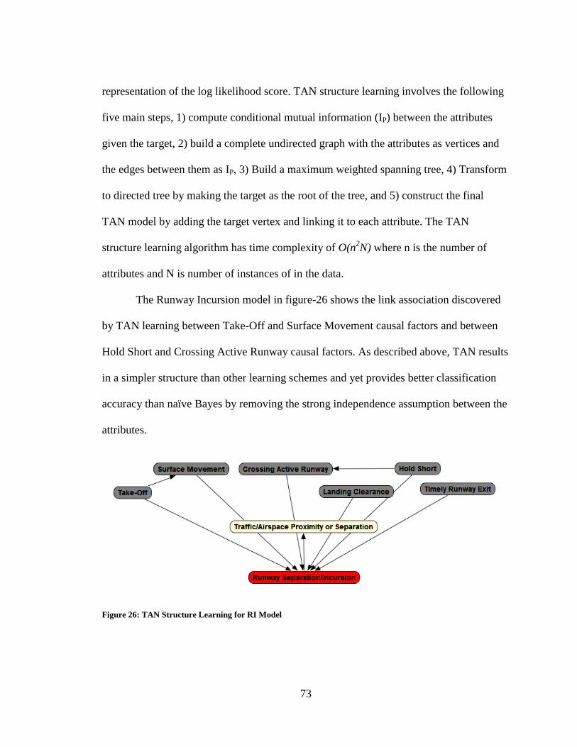
73
representation of the log likelihood score. TAN structure learning involves the following
five main steps, 1) compute conditional mutual information (IP) between the attributes
given the target, 2) build a complete undirected graph with the attributes as vertices and
the edges between them as IP, 3) Build a maximum weighted spanning tree, 4) Transform
to directed tree by making the target as the root of the tree, and 5) construct the final
TAN model by adding the target vertex and linking it to each attribute. The TAN
structure learning algorithm has time complexity of O(n2N) where n is the number of
attributes and N is number of instances of in the data.
The Runway Incursion model in figure-26 shows the link association discovered
by TAN learning between Take-Off and Surface Movement causal factors and between
Hold Short and Crossing Active Runway causal factors. As described above, TAN results
in a simpler structure than other learning schemes and yet provides better classification
accuracy than naïve Bayes by removing the strong independence assumption between the
attributes.
Figure 26: TAN Structure Learning for RI Model

74
3.5. Ranking of Common Factors As described in prior sections, the identification of top causal factors is in relation
to individual events, i.e. the algorithms rely on conditional probabilities of the causal
factors given the particular event. As a result, although they provide critical information
as to what factors contribute primarily to individual events, they don’t specify about the
generic issues in the NAS. Identifying common factors (generic issues) from data is so
important to communicate safety issues to the public and officials who are not
particularly concerned in the assessment of individual events but the overall risk in the
NAS for the flying public. This section describes how the common factors can be
identified from all the top causal factors that play a significant role in causing and
contributing to all event types.
Most quantitative risk management processes involve identifying individual
hazards and factoring the severity and occurrences or “likelihood” of those hazards. In
aviation risk management, severity is a measure of the effect of any particular hazard on
the safety of operation. It is measured by a numerical index to quantify the relative risk of
each hazard. For instance, for the purpose of determining accident risk in the NAS, the
FAA safety office uses a risk matrix based on five severity indices, 1- Catastrophic, 2-
Hazardous, 3-Major, 4-Minor, and 5-Minimal. Each of these indices is determined in
relation to its severity in different domains, such as the ATC services, flight operations,
and the flying public. Occurrences on the other hand deal with the “likelihood” of a
particular hazard in relation to some frequency measure. For instance, in aviation safety
risk management, occurrence is defined as the ratio of the number of a given hazard to
the number of operations or total flight hours for a specific time frame. The severity and

75
the occurrence together are used to quantify the risk in relation to some baseline
determined using domain knowledge. For the setting in this research, we can apply a
similar concept to rank the common or generic ATC-related factors in the NAS from the
top causal factors identified for individual events.
In this research, we deal with incidents instead of hazards, but each incident has
associated severity index assigned to it. As a result we can’t simply use number of
operations as a “likelihood” measure since not every incident is a hazard to aviation
safety. However, we can use the relative frequency of each causal factor given the
severity index as a similar measure. Using K severity indices, relative frequency of a top
causal factor, and the number of incidents from each category, the weight of each causal
factor can be determined by the following measure,
∑
⁄
In this expression, is the ith
factor, is the jth
severity index, and is the
number of events with jth
severity that the ith
causal factor is involved in. In this setting,
we are assuming that every event regardless of its type is weighted equally as long as it is
in the same severity class. That is, a Runway Incursion event has the same severity
weight as a Wake Turbulence event if the two have the same severity classification. This
assumption might not hold true in some cases as people tend to consider certain types of
events as more serious and consequential than others even with the same severity index.
3.6. Relationships of Events and Top Causal Factors over Time The sensitivity analysis and performance measure of each event model allow us to
identify the current top causal factors based on historical data, in a sense it is the snapshot
76
of the current causal factors for the given event. However, it doesn’t tell us how the
relationship between the top causal factors and the event behaved through time. In
dynamic systems such as the NAS, the characteristics of the data change overtime
reflecting the current state of the system. In standard Bayesian network learning we
consider every record in the training set with equal weight which comes from the
assumption that our observations have been produced by a stationary stochastic process.
For networks in dynamic problems we need to introduce a mechanism to adapt to the
changing system. One way of simulating a changing environment is using adapting
learning (Nielsen & Nielsen, 2008) by relaxing the assumption of stationary data to
piecewise stationary. Another simpler approach of adaptation which can be achieved at
the parameter estimation level is through the use of fading which involves assigning
different weight factors for training cases based on time. Using smaller weights for past
experiences and higher weights for recent observations we can make the model represent
more the current state of the system.
In this research I apply a different technique to gauge the extent to which the data
generating process has been changing for each undesired event. Using the top causal
factors identified from the full dataset, I export a weighted impact of each factor over
time. The data output used for this analysis maybe the monthly or quarterly distribution
of the top causal factors along with the impact, which is the change of probability as a
result of providing evidence on the undesired event, as a weight. For instance, for n top
causal factors { } and the impact of each as weights { }, the
weighted average of the top causal factors is given by,
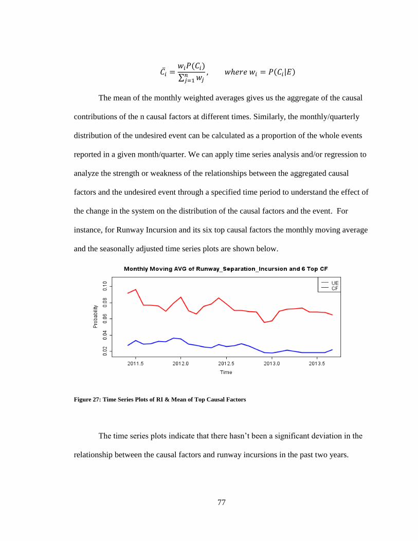
77
( )
∑
( | )
The mean of the monthly weighted averages gives us the aggregate of the causal
contributions of the n causal factors at different times. Similarly, the monthly/quarterly
distribution of the undesired event can be calculated as a proportion of the whole events
reported in a given month/quarter. We can apply time series analysis and/or regression to
analyze the strength or weakness of the relationships between the aggregated causal
factors and the undesired event through a specified time period to understand the effect of
the change in the system on the distribution of the causal factors and the event. For
instance, for Runway Incursion and its six top causal factors the monthly moving average
and the seasonally adjusted time series plots are shown below.
Figure 27: Time Series Plots of RI & Mean of Top Causal Factors
The time series plots indicate that there hasn’t been a significant deviation in the
relationship between the causal factors and runway incursions in the past two years.
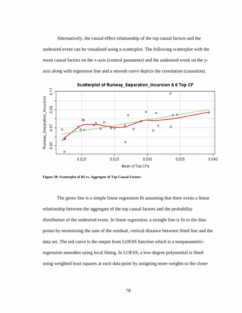
78
Alternatively, the causal-effect relationship of the top causal factors and the
undesired event can be visualized using a scatterplot. The following scatterplot with the
mean causal factors on the x-axis (control parameter) and the undesired event on the y-
axis along with regression line and a smooth curve depicts the correlation (causation).
Figure 28: Scatterplot of RI vs. Aggregate of Top Causal Factors
The green line is a simple linear regression fit assuming that there exists a linear
relationship between the aggregate of the top causal factors and the probability
distribution of the undesired event. In linear regression, a straight line is fit to the data
points by minimizing the sum of the residual, vertical distance between fitted line and the
data set. The red curve is the output from LOESS function which is a nonparametric-
regression smoother using local fitting. In LOESS, a low-degree polynomial is fitted
using weighted least squares at each data point by assigning more weights to the closer
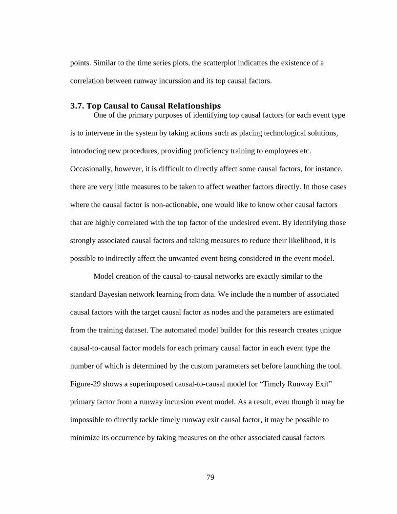
79
points. Similar to the time series plots, the scatterplot indicattes the existence of a
correlation between runway incurssion and its top causal factors.
3.7. Top Causal to Causal Relationships One of the primary purposes of identifying top causal factors for each event type
is to intervene in the system by taking actions such as placing technological solutions,
introducing new procedures, providing proficiency training to employees etc.
Occasionally, however, it is difficult to directly affect some causal factors, for instance,
there are very little measures to be taken to affect weather factors directly. In those cases
where the causal factor is non-actionable, one would like to know other causal factors
that are highly correlated with the top factor of the undesired event. By identifying those
strongly associated causal factors and taking measures to reduce their likelihood, it is
possible to indirectly affect the unwanted event being considered in the event model.
Model creation of the causal-to-causal networks are exactly similar to the
standard Bayesian network learning from data. We include the n number of associated
causal factors with the target causal factor as nodes and the parameters are estimated
from the training dataset. The automated model builder for this research creates unique
causal-to-causal factor models for each primary causal factor in each event type the
number of which is determined by the custom parameters set before launching the tool.
Figure-29 shows a superimposed causal-to-causal model for “Timely Runway Exit”
primary factor from a runway incursion event model. As a result, even though it may be
impossible to directly tackle timely runway exit causal factor, it may be possible to
minimize its occurrence by taking measures on the other associated causal factors
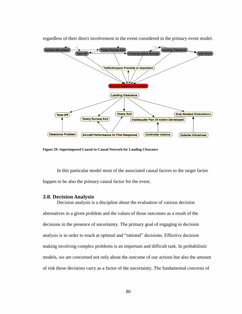
80
regardless of their direct involvement in the event considered in the primary event model.
Figure 29: Superimposed Causal-to-Causal Network for Landing Clearance
In this particular model most of the associated causal factors to the target factor
happen to be also the primary causal factor for the event.
3.8. Decision Analysis Decision analysis is a discipline about the evaluation of various decision
alternatives in a given problem and the values of those outcomes as a result of the
decisions in the presence of uncertainty. The primary goal of engaging in decision
analysis is in order to reach at optimal and “rational” decisions. Effective decision
making involving complex problems is an important and difficult task. In probabilistic
models, we are concerned not only about the outcome of our actions but also the amount
of risk those decisions carry as a factor of the uncertainty. The fundamental concerns of
81
decision analysis are weighing the probability of an event and the value of the
probabilistic outcome of our actions in relation to the event to determine the consequence
of our choices.
Various techniques and mathematical models are used in decision analysis to
maximize the value of the outcomes as a consequence of our decisions. Such models are
comprised of different components such as the events which are governed by nature, the
circumstances under which the decision are made, the set of actions, and the final
outcome or return of the interactions of those components. Each component has a source
of error which contributes to the uncertain outcome of the decision making process. Some
of the sources of errors are, partial understanding of the circumstances, incorrect
assumptions, the utility function used to measure the value of each outcome, and
forecasting errors.
Figure 30: Components of a Decision Model
Model
Actions
Events
Output
Assumptions

82
The domains of most mathematical decision models fall between two extreme
ends based on our level of knowledge in the problem domain and the circumstances that
govern it. On one end we have a pure uncertain model as a result of our complete
ignorance and on the other end we have a deterministic model due to our complete
knowledge. What lie in between are most models which are probabilistic due to our
partial knowledge.
3.8.1. Causal Bayesian Networks The only requirement in standard Bayesian networks is that the structure needs to
represent the underlying joint distribution correctly and answer probabilistic queries. The
direction of links between nodes in standard Bayesian networks don’t need to encode
causality, they may only represent correlations. When the directions of links are
significant, Bayesian networks can encode the causal relationship of one variable to
another and such networks are called causal models. In causal Bayesian networks, the
value of each variable is probabilistically governed by the values of its parents. For
instance, in our Runway Incursion model, take-off clearance is a causal factor to RI event
and such relationship is depicted by the fact that the direction of the link is towards the
effect variable.
Without some level of domain knowledge identifying causality is generally a
challenging problem. Given two correlated variables X and Y, it may be the case that X
causes Y, Y causes X or both may be correlated as a result of one or more external
observable or unobservable variables acting on them. For the purpose of answering
probabilistic queries, it is not necessary that we need to explicitly encode the
83
unobservable variables as long as the model captures the marginal distribution over the
observable variables. However, in causal model we need to identify the true source of the
cause for an effect in order to answer causal queries.
3.8.2. Intervention in Causal Models Causal models lend themselves to intervention which refers to an action taken to
force one or more causal variables to take a certain state. When we intervene and do
actions to force variables take certain values as opposed to observed values, the
intervention queries are explained using ‘do-calculus’ which is due to Judea Pearl, (Pearl,
1995). For instance, when we intervene in the RI causal model, we may take some
measures and fix take-off clearance problem and force its state to be “Not Factor”
signifying that it is no longer a cause for the target event. This results in a different
network from which the take-off causal factor is removed and the intervention query is
done as follows.
( | ( ( ) ) ( | )
In the above expression the assumption is that the causal relationship between
take-off clearance and RI event is entirely due to the correlation between the two
variables, i.e. there are no other hidden variables that are common to them and contribute
to their correlations. However, if we don’t assume that no hidden causes exist for the
causality, answering intervention query involves disentangling the effect of the hidden
variables which is generally a more difficult task. Pearls ‘do-calculus’ deals with actions
that result in a forced state with probability 1.0, perfect interventions. In reality, however,

84
fixing a take-off clearance may involve taking multiple actions and each of such actions
results in a certain level of reduction in the likelihood of the occurrence of the RI event.
3.8.3. Utilities in Decision Making In a decision making setting, there may be one or more possible actions with
different degrees of preferences by the decision maker and each action leads to a different
set of outcomes. In simple cases, each action results in one or more outputs with
certainty, and the appropriate action is selected in relation to the preferred outcome.
However, in real world problems, outcomes of an action or set of actions result in
complex set of outcomes distributed probabilistically. As a result, we need a numerical
measure to give a relative weighting of the different outcomes according to our
preferences, a higher weight to a preferred outcome and a lesser one to least preferred
outcome. In decision theory, the formal metric to measure such weighted outcomes is a
utility function.
The utility of an outcome is the numerical value of the outcome and a utility
function maps an action to a numerical value. In general, the higher the value of the
outcome, the preferred the action that leads to that outcome is. Numerical utilities allow
us to aggregate various probabilistic outcomes in order to reach the most preferred action.
In most practical decision making, the numerical utility values are significant and are
used to measure the relative strength of each outcome and such utilities are called
cardinal utilities. In ordinal utilities, we are not concerned about the relative numerical
values of each utility; we are merely interested in some kind preference ordering. The
85
probabilistic outcome of an action or set of actions are combined using expected utility
and the actions are ranked according to their expected utilities.
3.8.4. Utility Functions The use of utility in decision theory originated from economics, and it refers to
the perceived value of a good. In any utility-based decision making process, it is the
numerical value of the outcome of a decision. We need a mathematical function to map
the different outcomes as a result of our preferred decision choice to a numerical value.
Such functions are called utility functions and they are measurable functions on a
probability space. Although the use of utility function was suggested first by Bernoulli in
1738 to solve the St Petersburg Paradox1, the theory and the associated axioms of utility
function were further developed by von Neumann and Morgenstern in 1944. A utility
function is defined as,
Let X be a set of preferences, ≿ be preference relation, i.e. x ≿ y implies that x is the
preferred choice or the decision maker is indifferent between x and y,
For decision making in one variable,
≿ ( ) ( )
For decision making in multiple variables,
( ) ( )
( ) ≿ ( ) ( ) ( )
An important characteristic of a utility function is that it is an increasing function,
the higher the utility value the preferred the decision that leads to that output is.
1 A game of chance in which a fair coin is tossed repeatedly and a single player pays some fee doubling
every time a head appears. The game ends, and the player wins when a tail appears.
86
( )
However, after achieving certain level of utility values, the utility increase is
smaller making the utility curve concave, and such phenomenon is called decreasing
marginal utility.
( )
In minimizing the likelihood of decreasing an undesired event, for instance, the
actions we take on the various causal factors have higher effect (higher utility) towards
the initial stages of our actions than the final stages. Once we achieved a level of event
reduction, our actions in addressing more causal factors have lesser effects and it is
unlikely that we can completely eliminate the chance of event occurring due to other
external factors that are not directly attributable to factors we have direct control over.
3.8.5. The Effect of Risk on Utility Function Decision makers always need to take into consideration the risk involved when
arriving at a decision. A situation in which there are potential life loss and public safety
risks is taken much more seriously than a situation where only financial losses or gains
are in play. Also, evaluating the decision and determining the utility of each outcome in
high risk situations are much more difficult. Some of the models in this research involve
potentially high risk events such as serious runway incursions, loss of separations,
operational deviations etc. that could lead to potential accidents. However, for the
purpose of making decisions, the risks involved in this setting are not only related to the
severity of the event, they also involve the amount of scarce resources needed to be
allocated to minimize the likelihood of the undesired events. As a result, the utility
87
evaluation in this setting should weigh the risk of implementation of placing system or
procedural changes, mitigation strategies, and the risk of events occurring, severe and
less severe.
In the presence of risk, the selection of the utility function depends on the level of
risk aversion or risk seeking the decision makers would like to assume. As a result, there
is no single utility function that satisfies the preference of every decision maker even
under the same circumstances. However, in applying expected utility maximization, it is
assumed that every decision maker acts rationally in accordance with the four axioms of
utility theory.
The most common utility function in the presence of risk is exponential function
primarily due to its convenience in the computation.
( ) , α > 0
Computing the expected utility using an exponential utility function is equivalent
to calculating the moment generating function of a given variable. For instance, assume
that the allocated monitory resource to resolve one of the causal factors, R, as a random
variable and the decision maker uses exponential utility to measure the outcome in the
reduction of the event.
[ ( )] [ ] ( )
Assume that allocating increasingly more resources to resolve a causal factor will
reduce a given undesired event. As a result, the more resource we allocate, the higher the
utility becomes. However, after a certain level of reduction of the undesired event is
achieved, allocating more resources in addressing the same causal factor has increasingly
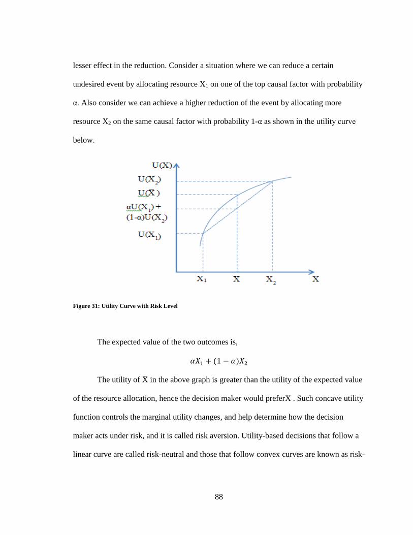
88
lesser effect in the reduction. Consider a situation where we can reduce a certain
undesired event by allocating resource X1 on one of the top causal factor with probability
α. Also consider we can achieve a higher reduction of the event by allocating more
resource X2 on the same causal factor with probability 1-α as shown in the utility curve
below.
Figure 31: Utility Curve with Risk Level
The expected value of the two outcomes is,
( )
The utility of X in the above graph is greater than the utility of the expected value
of the resource allocation, hence the decision maker would preferX . Such concave utility
function controls the marginal utility changes, and help determine how the decision
maker acts under risk, and it is called risk aversion. Utility-based decisions that follow a
linear curve are called risk-neutral and those that follow convex curves are known as risk-
89
seeking. However, most utility curves are linear locally and assume risk neutrality for
sufficiently small risk and benefits.
3.8.6. Expected Utility An action can have multiple consequences or outcomes based on the realization of
the target event. In “rational” decision making, the desired outcome can be achieved by
maximizing the expected utility in which the utility value of each outcome is measured
using utility function and the realization of the event is distributed probabilistically. The
theoretical justification for using the principle of expected utility as a definition of
“rational” behavior of the decision maker is rooted in the axioms of utility (von Neumann
& Morgenstern, 1944). According to utility theorem, for a decision maker who abides by
the axioms, there exists a utility function such that his or her decision is equivalent to the
maximum expected utility relative to the utility function. The four axioms of utility
theory are,
Completeness: for outcomes o1 and o2, the decision maker must be able to prefer one,
two or consider them equivalent.
| |
Transitivity: for outcomes o1, o2, and o3, if the decision maker prefers one to two and
two to three, he also prefers one to three.
Continuity: for outcomes o1, o2, o3 and probability α, if the decision maker prefers one to
two and two to three, then there is a possible combination of one and three with equal
preference with two.
90
[ ( )], α ϵ (0,1)
Independence: for outcomes o1, o2, o3 and probability α, if the decision maker has equal
preference for one and two, then the third can be combined with either without changing
the preferred outcome.
[ ( )] [ ( )]
The central theme of expected utility principle is that the highest expected utility
as opposed to expected value is used as the basis for the preferred outcome. Therefore,
for n possible outcomes O of an action A the expected utility EU is the sum of the product
of the utility function and the probability of each outcome.
∑ ( ( | ) ( | ))
It is expressed as a linear combination of the utilities of each outcome where the
weights are given by their respective probabilities. In the runway incursion model, for
instance, the possible alternative actions are, full control, partial control, or no control of
one of the causal factors, and the possible outcomes are reduction of runway incursion
and no reduction in the occurrence of runway incursions.
3.8.7. Graphical Representation of Decision Analysis Decision network, also known as influence diagram, is a structured representation
of a decision making process, it is an extension of a Bayesian network. It is a directed
acyclic graph consisting of three types of nodes—chance, decision, and utility nodes.
Like a Bayesian network, the chance nodes represent the random variables and their
values are governed by nature. The values of the decision nodes are directly controlled by
the decision maker reflecting his/her choice of preferences among the competing
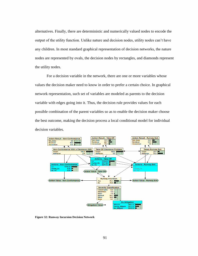
91
alternatives. Finally, there are deterministic and numerically valued nodes to encode the
output of the utility function. Unlike nature and decision nodes, utility nodes can’t have
any children. In most standard graphical representation of decision networks, the nature
nodes are represented by ovals, the decision nodes by rectangles, and diamonds represent
the utility nodes.
For a decision variable in the network, there are one or more variables whose
values the decision maker need to know in order to prefer a certain choice. In graphical
network representation, such set of variables are modeled as parents to the decision
variable with edges going into it. Thus, the decision rule provides values for each
possible combination of the parent variables so as to enable the decision maker choose
the best outcome, making the decision process a local conditional model for individual
decision variables.
Figure 32: Runway Incursion Decision Network
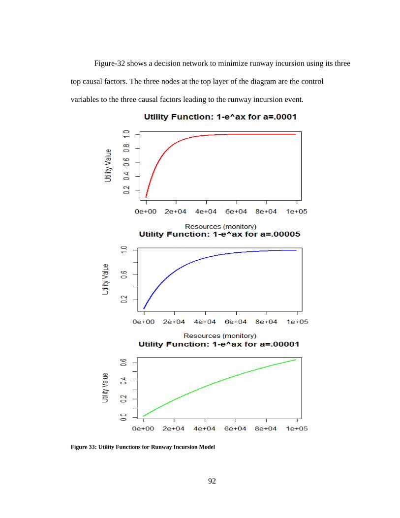
92
Figure-32 shows a decision network to minimize runway incursion using its three
top causal factors. The three nodes at the top layer of the diagram are the control
variables to the three causal factors leading to the runway incursion event.
Figure 33: Utility Functions for Runway Incursion Model
93
The control variables are functions of the result of the three serial actions, cyan
nodes, of the decision maker and distribution of the causal factors. The green diamond
nodes are the utility nodes to measure the probability of the Runway Incursion event and
the choice of the decision maker on the action nodes.
Similarly, we have a utility node and an action to the mitigation variable to affect
the consequence of the incident in the event it occurs. The functions to measure the utility
of each output as a result of our actions are shown in figure-33, they are meant to be
experimental values. In actual decision making those values are determined based on
additional factors that are available to the decision maker.
3.9. Automated Model Creation In large networks, creating the DAG and the local CPDs manually can be very
tedious. Although there are various packages with easier user interfaces for creating
nodes, connecting edges, and entering the local CPDs, building large networks manually
can still be very laborious task. For this project, I have compiled various software
packages such as, R, WEKA, NETICA, and connected them using a custom java program
that generates the network and the various components of the models explained
throughout this paper without the need to manual interventions. An XML-based
configuration file, which is exported from the database schema, contains information
such as the name of the variables, parent variables, relative location, and the hierarchal
structure entirely reflects those relationships. The CPDs for each variable are populated
from the training data file using frequency count, and the performance is validated
against the test dataset.
94
4. RESEARCH ANALYSES
This section describes the results of an analysis using the algorithms described in
chapter 3 (Methodology) on the ATSAP data. The analysis was conducted using ATSAP
data from May 2011 to October 2013. This period coincides with the ATSAP taxonomy
structure that includes 21 event types and more than 300 causal factors. The incidents are
classified under three categories: Proximity/Separation Issues, Unexpected Conditions,
and Aircraft Accident, and the factors are grouped into 15 high-level categories. The
various causal models were trained using 35,000 event records that comprise a total of
41,000 incident reports. Although the large majority of events are distinct events, there
are some overlaps between separation and unexpected condition events. That is, some
separation problems also involve unexpected conditions. Consequently, it is required that
we treat each event as a separate Bernoulli variable for the purpose of identifying its
causal factors and their correlations given the event.
This section is organized as follows: section 4.1 summarizes the list of events
with their relative frequency and severity. Section 4.2 summarizes the significant causal
factors for each event as identified by the probabilistic causal models. Section 4.3
explains some of the reasoning behind the high variations in correlation between
significant factors and few of the events over time in. Section 4.4 describes the top-n
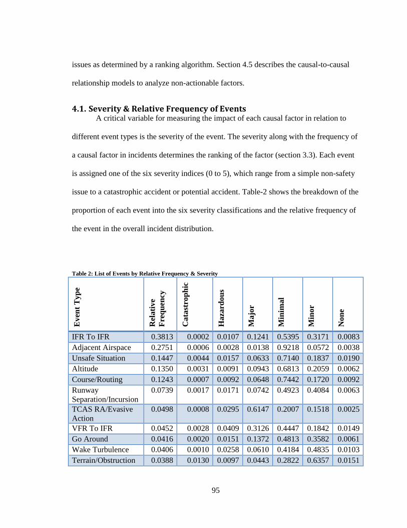
95
issues as determined by a ranking algorithm. Section 4.5 describes the causal-to-causal
relationship models to analyze non-actionable factors.
4.1. Severity & Relative Frequency of Events A critical variable for measuring the impact of each causal factor in relation to
different event types is the severity of the event. The severity along with the frequency of
a causal factor in incidents determines the ranking of the factor (section 3.3). Each event
is assigned one of the six severity indices (0 to 5), which range from a simple non-safety
issue to a catastrophic accident or potential accident. Table-2 shows the breakdown of the
proportion of each event into the six severity classifications and the relative frequency of
the event in the overall incident distribution.
Table 2: List of Events by Relative Frequency & Severity
Even
t T
yp
e
Rel
ati
ve
Fre
qu
ency
Cata
stro
ph
ic
Haza
rdou
s
Majo
r
Min
imal
Min
or
Non
e IFR To IFR 0.3813 0.0002 0.0107 0.1241 0.5395 0.3171 0.0083
Adjacent Airspace 0.2751 0.0006 0.0028 0.0138 0.9218 0.0572 0.0038
Unsafe Situation 0.1447 0.0044 0.0157 0.0633 0.7140 0.1837 0.0190
Altitude 0.1350 0.0031 0.0091 0.0943 0.6813 0.2059 0.0062
Course/Routing 0.1243 0.0007 0.0092 0.0648 0.7442 0.1720 0.0092
Runway
Separation/Incursion
0.0739 0.0017 0.0171 0.0742 0.4923 0.4084 0.0063
TCAS RA/Evasive
Action
0.0498 0.0008 0.0295 0.6147 0.2007 0.1518 0.0025
VFR To IFR 0.0452 0.0028 0.0409 0.3126 0.4447 0.1842 0.0149
Go Around 0.0416 0.0020 0.0151 0.1372 0.4813 0.3582 0.0061
Wake Turbulence 0.0406 0.0010 0.0258 0.0610 0.4184 0.4835 0.0103
Terrain/Obstruction 0.0388 0.0130 0.0097 0.0443 0.2822 0.6357 0.0151
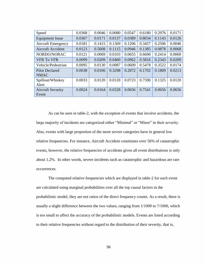
96
Speed 0.0368 0.0046 0.0080 0.0547 0.6180 0.2976 0.0171
Equipment Issue 0.0367 0.0171 0.0137 0.0389 0.8034 0.1143 0.0126
Aircraft Emergency 0.0181 0.1415 0.1369 0.1206 0.3457 0.2506 0.0046
Aircraft Accident 0.0123 0.5608 0.1115 0.0946 0.1385 0.0878 0.0068
NORDO/NORAC 0.0121 0.0069 0.0103 0.0655 0.6690 0.2414 0.0069
VFR To VFR 0.0099 0.0209 0.0460 0.0962 0.5816 0.2343 0.0209
Vehicle/Pedestrian 0.0095 0.0130 0.0087 0.0609 0.5478 0.3522 0.0174
Pilot Declared
NMAC
0.0038 0.0106 0.3298 0.2872 0.1702 0.1809 0.0213
Spillout/Whiskey
Alert
0.0033 0.0120 0.0120 0.0723 0.7590 0.1325 0.0120
Aircraft Security
Event
0.0024 0.0164 0.0328 0.0656 0.7541 0.0656 0.0656
As can be seen in table-2, with the exception of events that involve accidents, the
large majority of incidents are categorized either “Minimal” or “Minor” in their severity.
Also, events with large proportion of the more severe categories have in general low
relative frequencies. For instance, Aircraft Accident constitutes over 56% of catastrophic
events, however, the relative frequencies of accidents given all event distributions is only
about 1.2%. In other words, severe incidents such as catastrophic and hazardous are rare
occurrences.
The computed relative frequencies which are displayed in table-2 for each event
are calculated using marginal probabilities over all the top causal factors in the
probabilistic model, they are not ratios of the direct frequency counts. As a result, there is
usually a slight difference between the two values, ranging from 1/1000 to 7/1000, which
is too small to affect the accuracy of the probabilistic models. Events are listed according
to their relative frequencies without regard to the distribution of their severity, that is,
97
events with higher frequencies are listed first. Also, few of the events in the bottom list
have very small relative frequencies and hence the top causal factors identified for such
events are less reliable due to the number of incidents available to train the models. As a
result, events whose relative frequencies are less than 1% are excluded from the model
outputs in section 4.2. Accidents are also excluded from the result due to some of the
issues many raise as to whether or not the ATSAP program has the resources to analyze
accidents. FAA regulation requires that aviation accidents are investigated and analyzed
by the NTSB, and such investigation usually take longer time and much more resources.
4.2. Significant Causal Factors This section describes the outputs of the probabilistic causal models that are
generated to identify top causal factors for each event. The top causal factors are based on
individual events, i.e., they are factors which are significant in causing or contributing to
the individual safety events. As explained in sections above, the ranking of the causal
factors are based on the difference of prior probabilities and posterior probabilities of
each causal factor given a particular event. The larger the difference is the higher the
ranking of the factor. In addition, correlation between any pair of causal factors given the
learned structure of the network is indicated by a link between them with the direction of
the link signifying no causality between the pairs. The correlation between factors is a
result of the TAN structure learning described in partial structure learning section of
chapter 3. The output includes a list of the top causal factors, probabilistic networks, time
series plots, and scatterplots of the 15 events with computed relative frequency above
1%.
98
The tables show the listing of the significant causal factors for each event along
with the definition of the causal factor as adapted from the ATSAP data dictionary, the
prior probability which is the probability of the causal factor given all event types, and
the posterior probability which is the probability of the factor given the particular event
type. The posterior is calculated using message passing-based evidence propagation
algorithm of Bayesian networks (see section 2.3.8). The probabilistic networks are
represented in graphical models with incidents as target event variables, the factors
(features) as causal nodes, and the links that connect any pair of nodes with significant
correlation as determined by the structure learning algorithm. They also display the
probabilistic values of each causal factor to indicate the strength of the correlation. The
time series plots are used to assess the relationship of the aggregate of the top causal
factors and an event frequency over a two year period (2011 – 2013). The scatterplots
show visually the strength of the correlation of the aggregate top causal factors and event
frequencies. When there are relatively many diverging variations between the aggregate
factors and the event frequency, the relationship tends to be weaker which is shown on a
non-increasing curve on the scatterplot (see section 4.3 for explanation).
4.2.1. IFR to IFR IFR (Instrument Flight Rules) to IFR events are those that involve loss of standard
separation between two or more aircraft operating under IFR rules. In IFR rules, flying by
visual references are unsafe, and hence onboard instruments and electronic signals are
used for navigation. There are 6 significant causal or contributing factors for IFR to IFR
events as shown in table-3. The structure of the probabilistic model shows that there is a

99
relatively stronger correlation between “altitude clearance problem” and “action or plan
execution”. The time series plots between the aggregate of the top causal factors and the
event show that since mid-2012, the two are diverging suggesting that other factors, not
discovered in the model, were also playing role in causing or contributing to IFR to IFR
events. Similar to the time series plots, the scatterplot shows that there is a decreasing
correlation between the top causal factors identified and the event. If the trend continues,
a similarly built model will show a different set of top causal factors in the near future.
Table 3: IFR to IFR Top Causal Factors
Rank Causal Factor Description Prior Posterior
1 Clearance
Problem/Altitude
Issuing instruction other than
what was authorized or
intended 0.174 0.263
2 Controller Actions/Action
or Plan Execution
Execution of a particular action
and/or plan is poor/inadequate
for the situation 0.183 0.255
3 Controller
Actions/Inadequate Plan of
Action Developed
Risk was not recognized or
misjudged and the devised
action or plan by the individual
is inadequate for the situation 0.134 0.195
4 Clearance
Problem/Heading
Issuing a heading instruction
other than what was authorized
or intended 0.08 0.138
5 Aircraft Performance or
Pilot Response/Timely
Aircraft Descent or Climb
The combined performance of
the aircrew and the aircraft
capability results in an
untimely descent/climb 0.077 0.125
6 Aircraft Performance or
Pilot Response/Timely
Aircraft Turn
The combined performance of
the aircrew and the aircraft
capability results in an
untimely turn 0.059 0.099
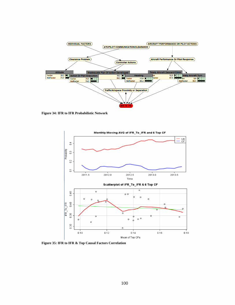
100
Figure 34: IFR to IFR Probabilistic Network
Figure 35: IFR to IFR & Top Causal Factors Correlation
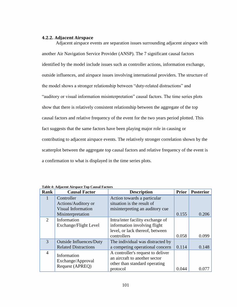
101
4.2.2. Adjacent Airspace Adjacent airspace events are separation issues surrounding adjacent airspace with
another Air Navigation Service Provider (ANSP). The 7 significant causal factors
identified by the model include issues such as controller actions, information exchange,
outside influences, and airspace issues involving international providers. The structure of
the model shows a stronger relationship between “duty-related distractions” and
“auditory or visual information misinterpretation” causal factors. The time series plots
show that there is relatively consistent relationship between the aggregate of the top
causal factors and relative frequency of the event for the two years period plotted. This
fact suggests that the same factors have been playing major role in causing or
contributing to adjacent airspace events. The relatively stronger correlation shown by the
scatterplot between the aggregate top causal factors and relative frequency of the event is
a confirmation to what is displayed in the time series plots.
Table 4: Adjacent Airspace Top Causal Factors
Rank Causal Factor Description Prior Posterior
1 Controller
Actions/Auditory or
Visual Information
Misinterpretation
Action towards a particular
situation is the result of
misinterpreting an auditory cue
0.155 0.206
2 Information
Exchange/Flight Level
Intra/inter facility exchange of
information involving flight
level, or lack thereof, between
controllers 0.058 0.099
3 Outside Influences/Duty
Related Distractions
The individual was distracted by
a competing operational concern 0.114 0.148
4 Information
Exchange/Approval
Request (APREQ)
A controller's request to deliver
an aircraft to another sector
other than standard operating
protocol 0.044 0.077
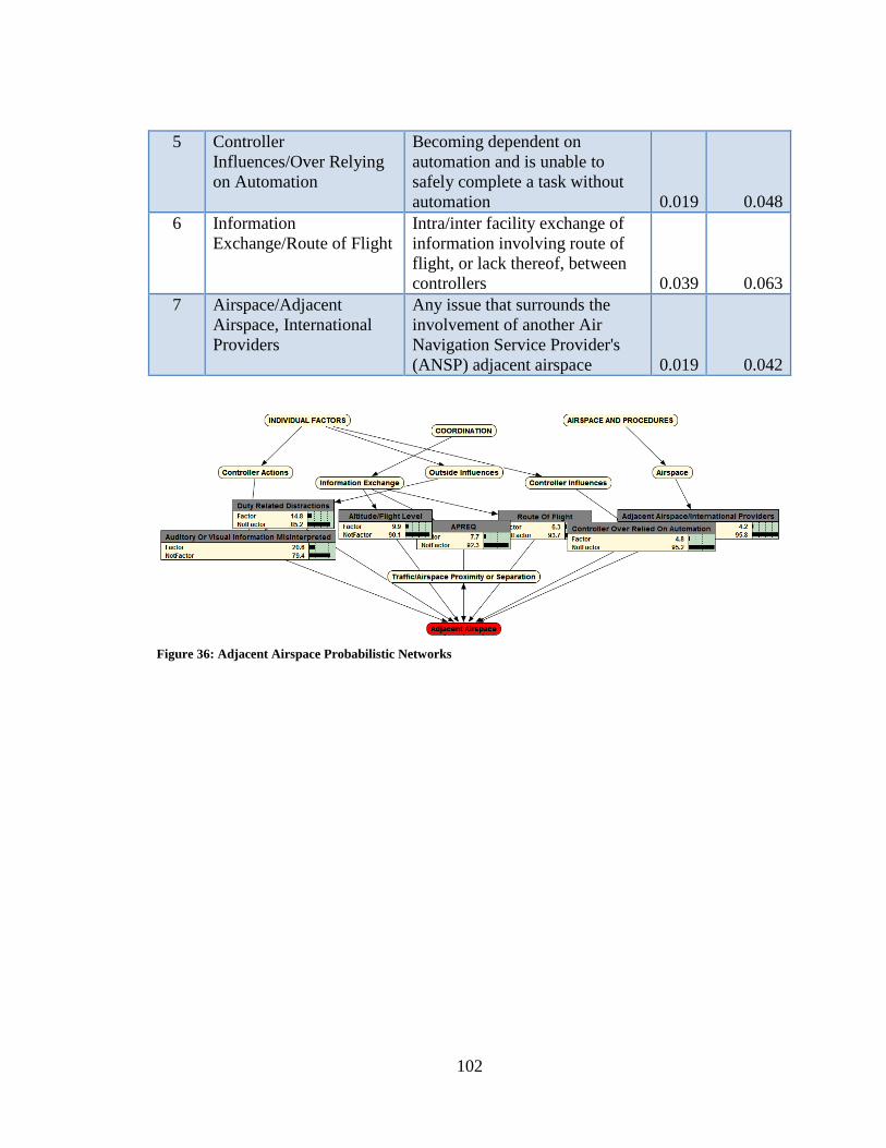
102
5 Controller
Influences/Over Relying
on Automation
Becoming dependent on
automation and is unable to
safely complete a task without
automation 0.019 0.048
6 Information
Exchange/Route of Flight
Intra/inter facility exchange of
information involving route of
flight, or lack thereof, between
controllers 0.039 0.063
7 Airspace/Adjacent
Airspace, International
Providers
Any issue that surrounds the
involvement of another Air
Navigation Service Provider's
(ANSP) adjacent airspace 0.019 0.042
Figure 36: Adjacent Airspace Probabilistic Networks
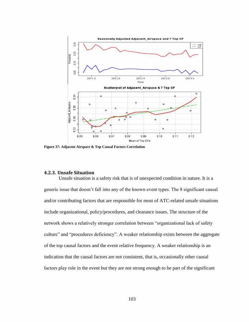
103
Figure 37: Adjacent Airspace & Top Causal Factors Correlation
4.2.3. Unsafe Situation Unsafe situation is a safety risk that is of unexpected condition in nature. It is a
generic issue that doesn’t fall into any of the known event types. The 8 significant causal
and/or contributing factors that are responsible for most of ATC-related unsafe situations
include organizational, policy/procedures, and clearance issues. The structure of the
network shows a relatively stronger correlation between “organizational lack of safety
culture” and “procedures deficiency”. A weaker relationship exists between the aggregate
of the top causal factors and the event relative frequency. A weaker relationship is an
indication that the causal factors are not consistent, that is, occasionally other causal
factors play role in the event but they are not strong enough to be part of the significant
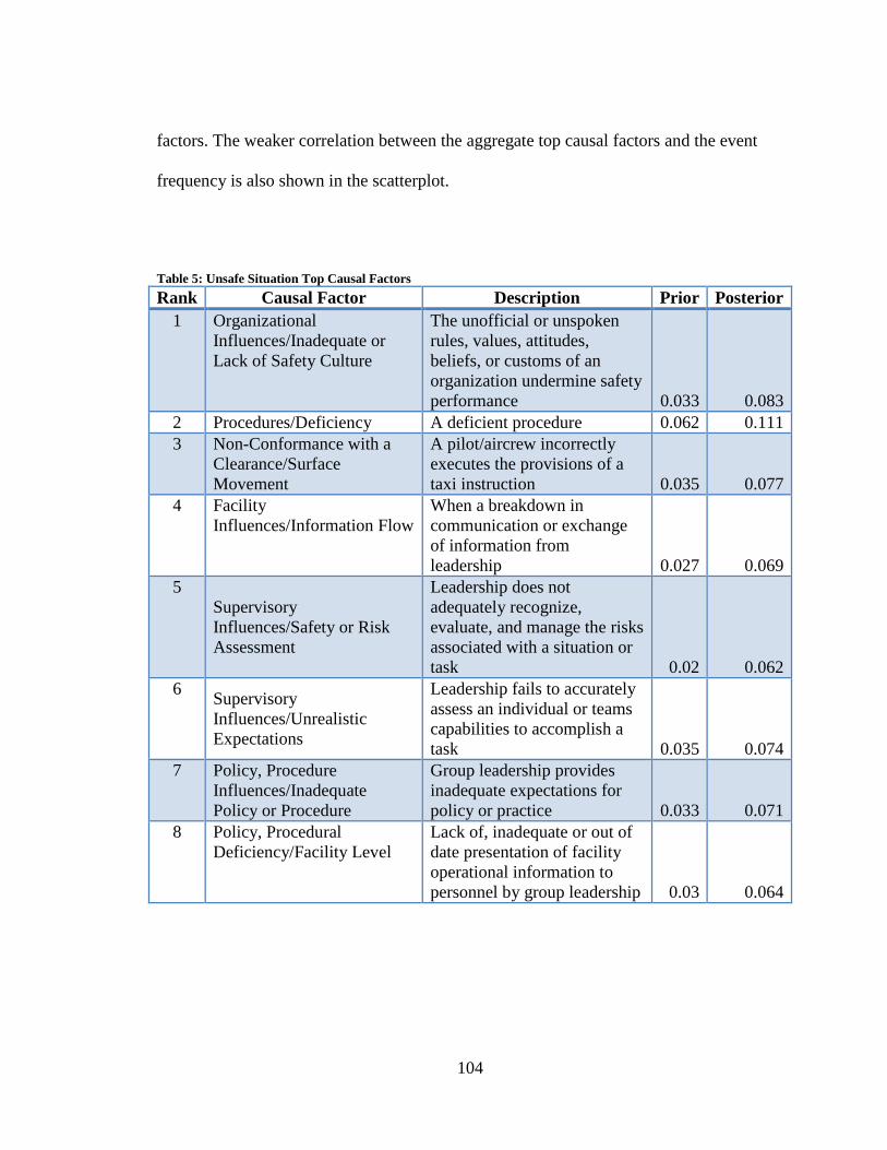
104
factors. The weaker correlation between the aggregate top causal factors and the event
frequency is also shown in the scatterplot.
Table 5: Unsafe Situation Top Causal Factors
Rank Causal Factor Description Prior Posterior
1 Organizational
Influences/Inadequate or
Lack of Safety Culture
The unofficial or unspoken
rules, values, attitudes,
beliefs, or customs of an
organization undermine safety
performance 0.033 0.083
2 Procedures/Deficiency A deficient procedure 0.062 0.111
3 Non-Conformance with a
Clearance/Surface
Movement
A pilot/aircrew incorrectly
executes the provisions of a
taxi instruction 0.035 0.077
4 Facility
Influences/Information Flow
When a breakdown in
communication or exchange
of information from
leadership 0.027 0.069
5
Supervisory
Influences/Safety or Risk
Assessment
Leadership does not
adequately recognize,
evaluate, and manage the risks
associated with a situation or
task 0.02 0.062
6 Supervisory
Influences/Unrealistic
Expectations
Leadership fails to accurately
assess an individual or teams
capabilities to accomplish a
task 0.035 0.074
7 Policy, Procedure
Influences/Inadequate
Policy or Procedure
Group leadership provides
inadequate expectations for
policy or practice 0.033 0.071
8 Policy, Procedural
Deficiency/Facility Level
Lack of, inadequate or out of
date presentation of facility
operational information to
personnel by group leadership 0.03 0.064
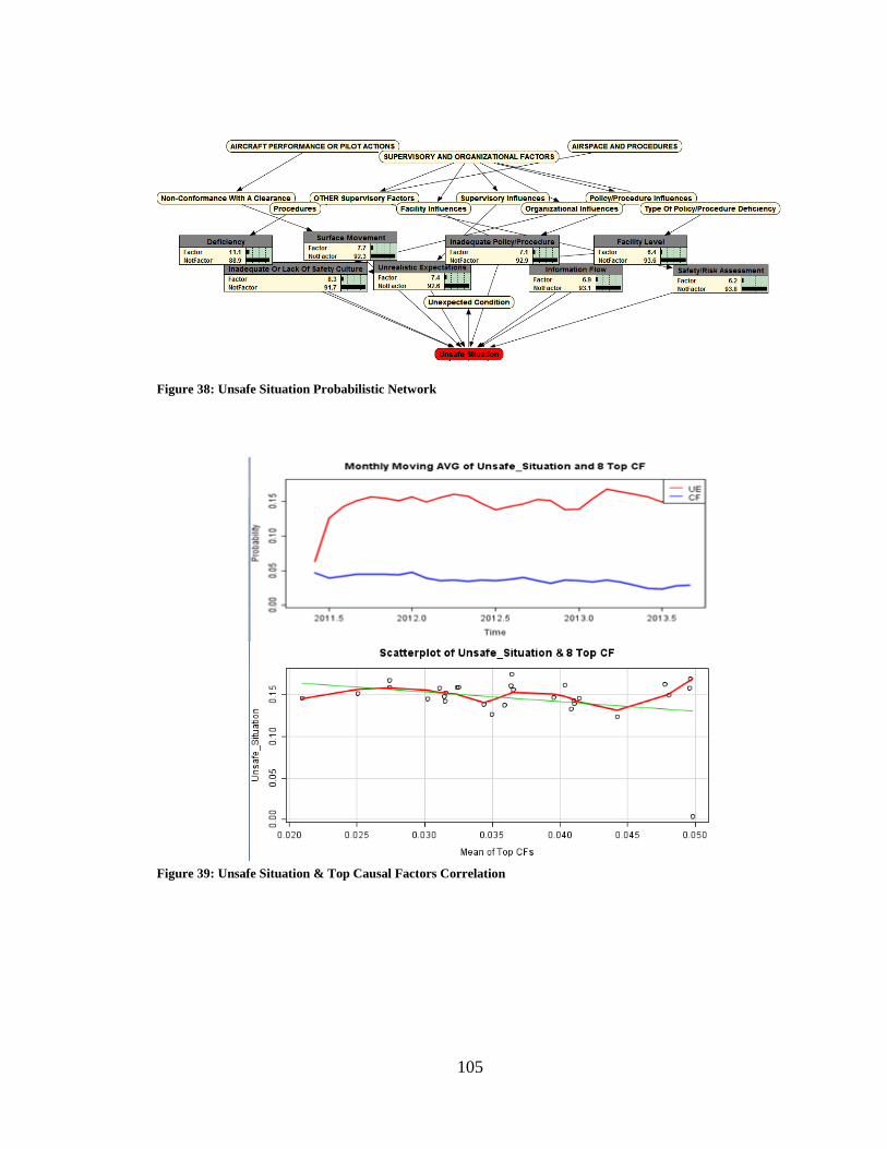
105
Figure 38: Unsafe Situation Probabilistic Network
Figure 39: Unsafe Situation & Top Causal Factors Correlation
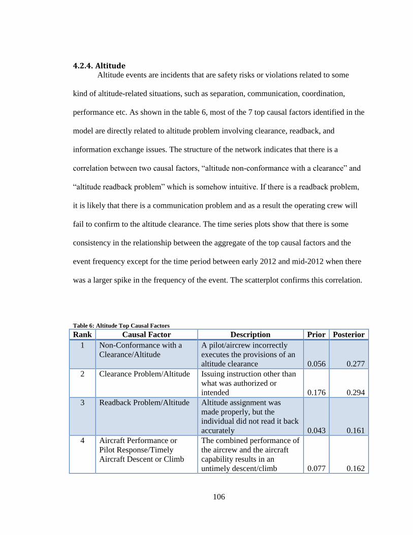
106
4.2.4. Altitude Altitude events are incidents that are safety risks or violations related to some
kind of altitude-related situations, such as separation, communication, coordination,
performance etc. As shown in the table 6, most of the 7 top causal factors identified in the
model are directly related to altitude problem involving clearance, readback, and
information exchange issues. The structure of the network indicates that there is a
correlation between two causal factors, “altitude non-conformance with a clearance” and
“altitude readback problem” which is somehow intuitive. If there is a readback problem,
it is likely that there is a communication problem and as a result the operating crew will
fail to confirm to the altitude clearance. The time series plots show that there is some
consistency in the relationship between the aggregate of the top causal factors and the
event frequency except for the time period between early 2012 and mid-2012 when there
was a larger spike in the frequency of the event. The scatterplot confirms this correlation.
Table 6: Altitude Top Causal Factors
Rank Causal Factor Description Prior Posterior
1 Non-Conformance with a
Clearance/Altitude
A pilot/aircrew incorrectly
executes the provisions of an
altitude clearance 0.056 0.277
2 Clearance Problem/Altitude Issuing instruction other than
what was authorized or
intended 0.176 0.294
3 Readback Problem/Altitude Altitude assignment was
made properly, but the
individual did not read it back
accurately 0.043 0.161
4 Aircraft Performance or
Pilot Response/Timely
Aircraft Descent or Climb
The combined performance of
the aircrew and the aircraft
capability results in an
untimely descent/climb 0.077 0.162
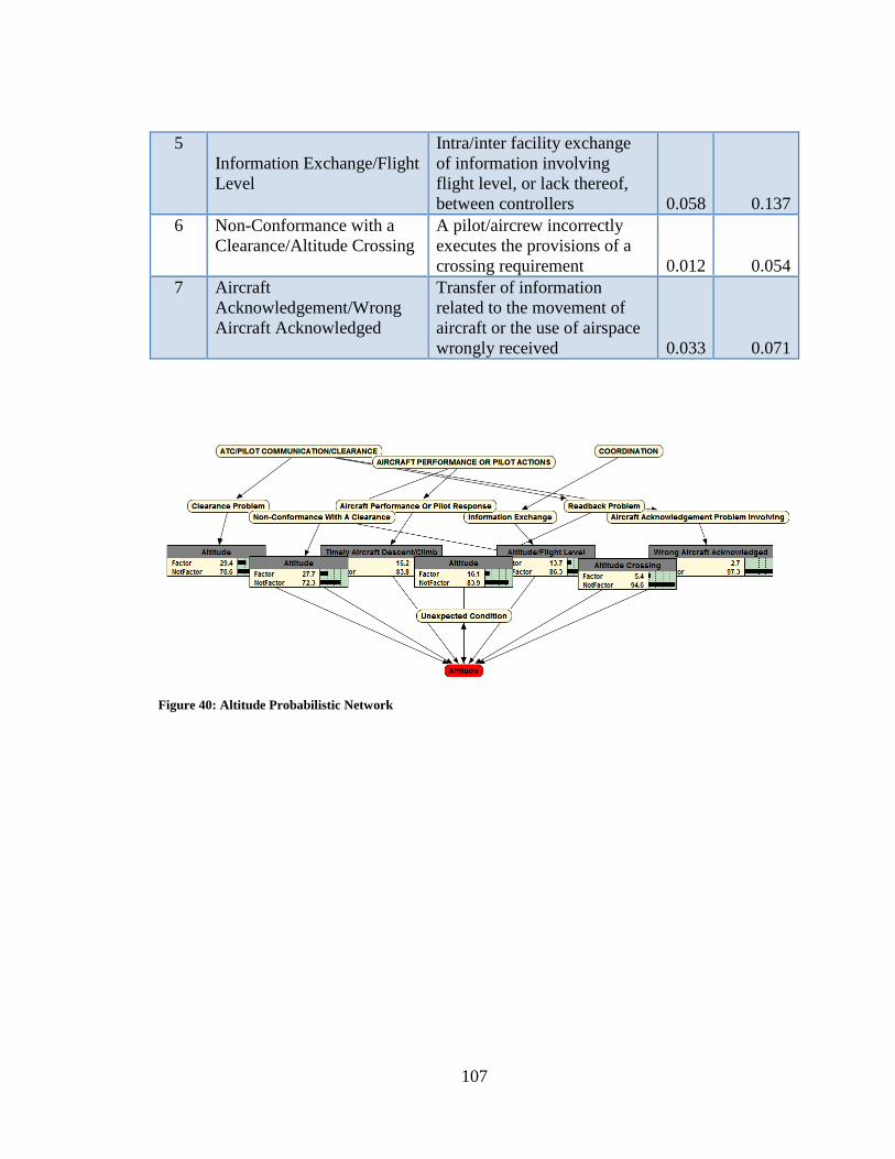
107
5
Information Exchange/Flight
Level
Intra/inter facility exchange
of information involving
flight level, or lack thereof,
between controllers 0.058 0.137
6 Non-Conformance with a
Clearance/Altitude Crossing
A pilot/aircrew incorrectly
executes the provisions of a
crossing requirement 0.012 0.054
7 Aircraft
Acknowledgement/Wrong
Aircraft Acknowledged
Transfer of information
related to the movement of
aircraft or the use of airspace
wrongly received 0.033 0.071
Figure 40: Altitude Probabilistic Network
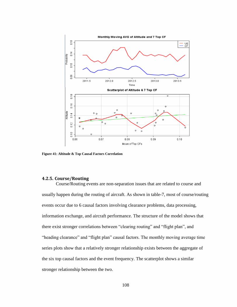
108
Figure 41: Altitude & Top Causal Factors Correlation
4.2.5. Course/Routing Course/Routing events are non-separation issues that are related to course and
usually happen during the routing of aircraft. As shown in table-7, most of course/routing
events occur due to 6 causal factors involving clearance problems, data processing,
information exchange, and aircraft performance. The structure of the model shows that
there exist stronger correlations between “clearing routing” and “flight plan”, and
“heading clearance” and “flight plan” causal factors. The monthly moving average time
series plots show that a relatively stronger relationship exists between the aggregate of
the six top causal factors and the event frequency. The scatterplot shows a similar
stronger relationship between the two.
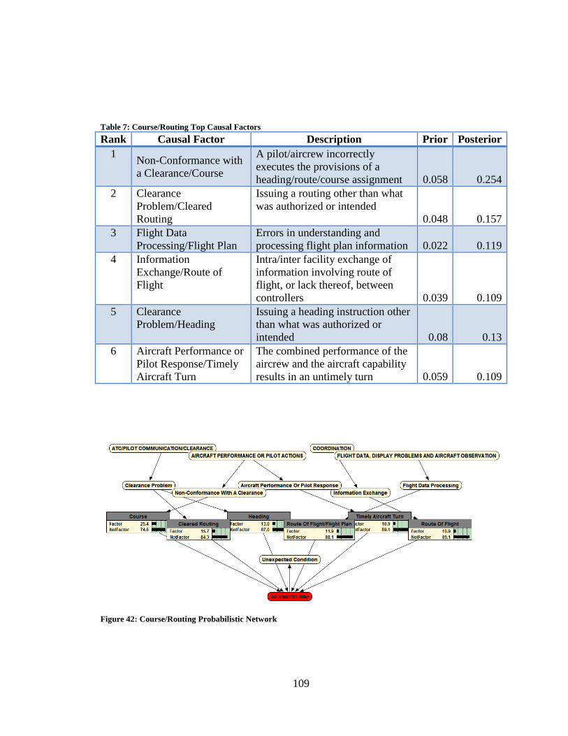
109
Table 7: Course/Routing Top Causal Factors
Rank Causal Factor Description Prior Posterior
1 Non-Conformance with
a Clearance/Course
A pilot/aircrew incorrectly
executes the provisions of a
heading/route/course assignment 0.058 0.254
2 Clearance
Problem/Cleared
Routing
Issuing a routing other than what
was authorized or intended
0.048 0.157
3 Flight Data
Processing/Flight Plan
Errors in understanding and
processing flight plan information 0.022 0.119
4 Information
Exchange/Route of
Flight
Intra/inter facility exchange of
information involving route of
flight, or lack thereof, between
controllers 0.039 0.109
5 Clearance
Problem/Heading
Issuing a heading instruction other
than what was authorized or
intended 0.08 0.13
6 Aircraft Performance or
Pilot Response/Timely
Aircraft Turn
The combined performance of the
aircrew and the aircraft capability
results in an untimely turn 0.059 0.109
Figure 42: Course/Routing Probabilistic Network
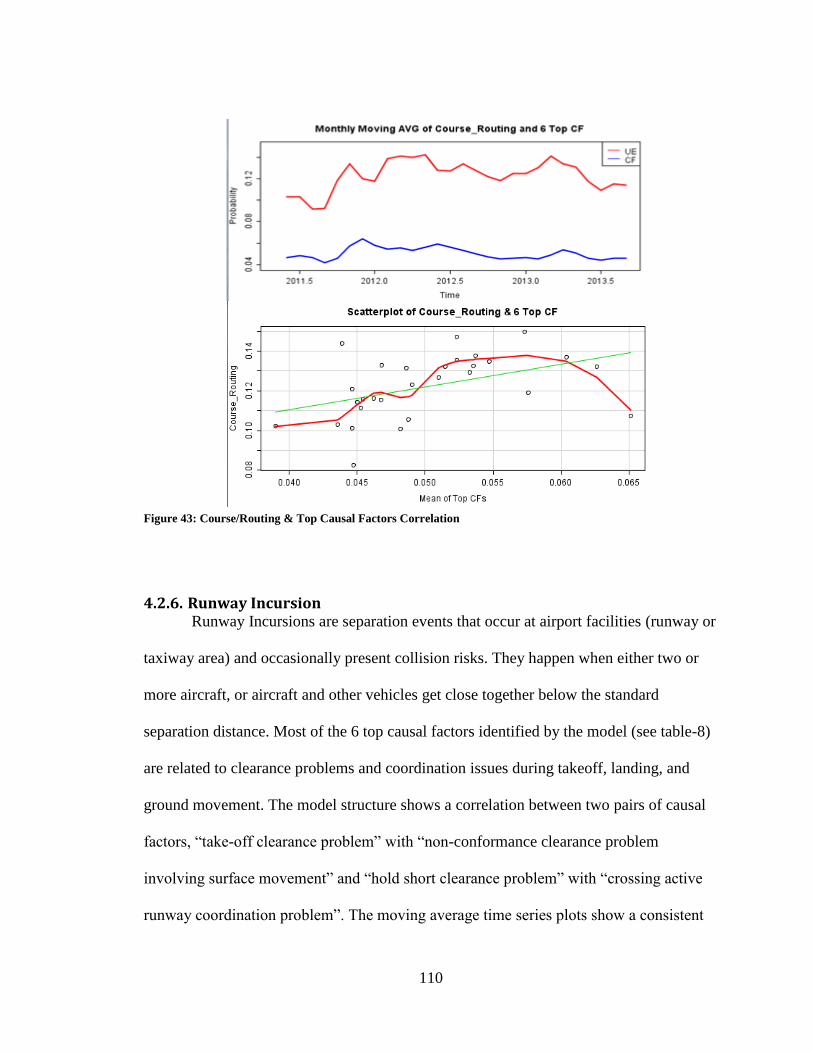
110
Figure 43: Course/Routing & Top Causal Factors Correlation
4.2.6. Runway Incursion Runway Incursions are separation events that occur at airport facilities (runway or
taxiway area) and occasionally present collision risks. They happen when either two or
more aircraft, or aircraft and other vehicles get close together below the standard
separation distance. Most of the 6 top causal factors identified by the model (see table-8)
are related to clearance problems and coordination issues during takeoff, landing, and
ground movement. The model structure shows a correlation between two pairs of causal
factors, “take-off clearance problem” with “non-conformance clearance problem
involving surface movement” and “hold short clearance problem” with “crossing active
runway coordination problem”. The moving average time series plots show a consistent
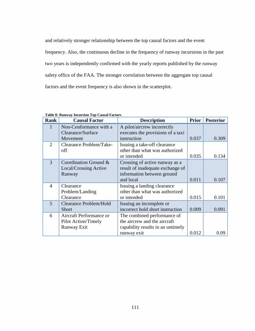
111
and relatively stronger relationship between the top causal factors and the event
frequency. Also, the continuous decline in the frequency of runway incursions in the past
two years is independently confirmed with the yearly reports published by the runway
safety office of the FAA. The stronger correlation between the aggregate top causal
factors and the event frequency is also shown in the scatterplot.
Table 8: Runway Incursion Top Causal Factors
Rank Causal Factor Description Prior Posterior
1 Non-Conformance with a
Clearance/Surface
Movement
A pilot/aircrew incorrectly
executes the provisions of a taxi
instruction 0.037 0.309
2 Clearance Problem/Take-
off
Issuing a take-off clearance
other than what was authorized
or intended 0.035 0.134
3 Coordination Ground &
Local/Crossing Active
Runway
Crossing of active runway as a
result of inadequate exchange of
information between ground
and local 0.011 0.107
4 Clearance
Problem/Landing
Clearance
Issuing a landing clearance
other than what was authorized
or intended 0.015 0.101
5 Clearance Problem/Hold
Short
Issuing an incomplete or
incorrect hold short instruction 0.009 0.091
6 Aircraft Performance or
Pilot Action/Timely
Runway Exit
The combined performance of
the aircrew and the aircraft
capability results in an untimely
runway exit 0.012 0.09
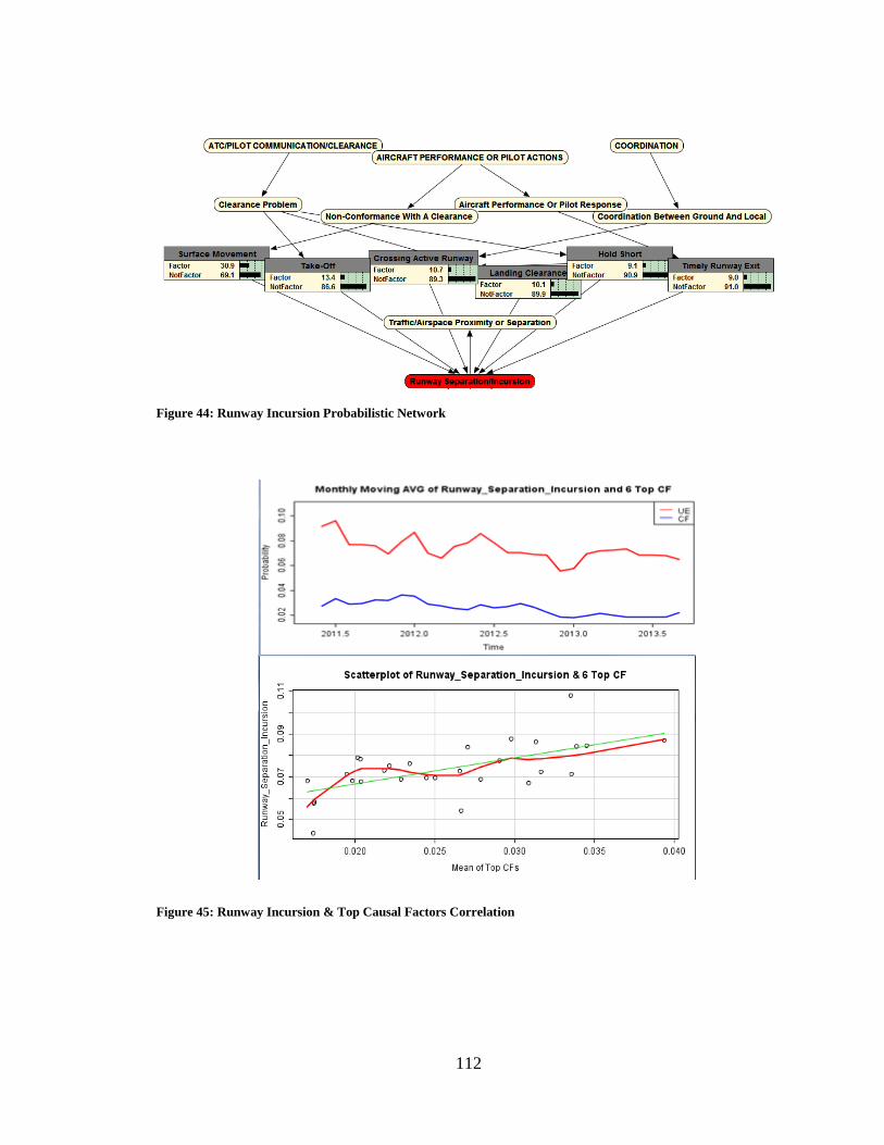
112
Figure 44: Runway Incursion Probabilistic Network
Figure 45: Runway Incursion & Top Causal Factors Correlation
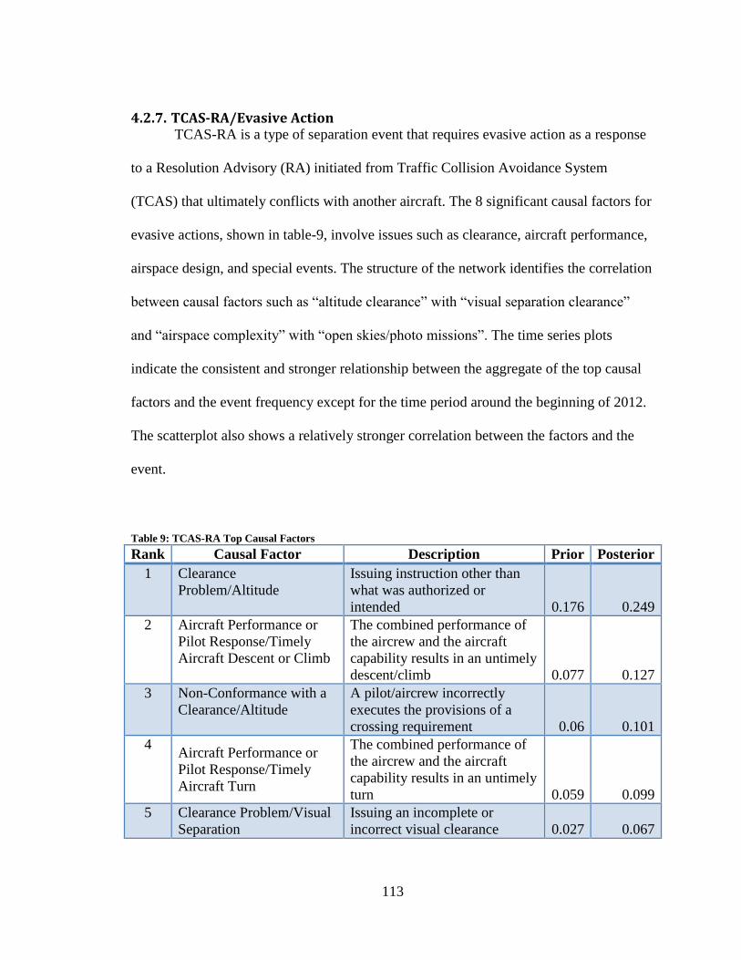
113
4.2.7. TCAS-RA/Evasive Action TCAS-RA is a type of separation event that requires evasive action as a response
to a Resolution Advisory (RA) initiated from Traffic Collision Avoidance System
(TCAS) that ultimately conflicts with another aircraft. The 8 significant causal factors for
evasive actions, shown in table-9, involve issues such as clearance, aircraft performance,
airspace design, and special events. The structure of the network identifies the correlation
between causal factors such as “altitude clearance” with “visual separation clearance”
and “airspace complexity” with “open skies/photo missions”. The time series plots
indicate the consistent and stronger relationship between the aggregate of the top causal
factors and the event frequency except for the time period around the beginning of 2012.
The scatterplot also shows a relatively stronger correlation between the factors and the
event.
Table 9: TCAS-RA Top Causal Factors
Rank Causal Factor Description Prior Posterior
1 Clearance
Problem/Altitude
Issuing instruction other than
what was authorized or
intended 0.176 0.249
2 Aircraft Performance or
Pilot Response/Timely
Aircraft Descent or Climb
The combined performance of
the aircrew and the aircraft
capability results in an untimely
descent/climb 0.077 0.127
3 Non-Conformance with a
Clearance/Altitude
A pilot/aircrew incorrectly
executes the provisions of a
crossing requirement 0.06 0.101
4 Aircraft Performance or
Pilot Response/Timely
Aircraft Turn
The combined performance of
the aircrew and the aircraft
capability results in an untimely
turn 0.059 0.099
5 Clearance Problem/Visual
Separation
Issuing an incomplete or
incorrect visual clearance 0.027 0.067
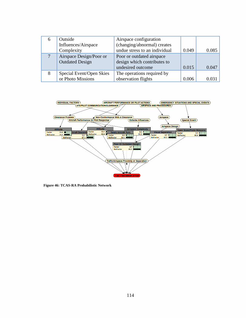
114
6 Outside
Influences/Airspace
Complexity
Airspace configuration
(changing/abnormal) creates
undue stress to an individual 0.049 0.085
7 Airspace Design/Poor or
Outdated Design
Poor or outdated airspace
design which contributes to
undesired outcome 0.015 0.047
8 Special Event/Open Skies
or Photo Missions
The operations required by
observation flights 0.006 0.031
Figure 46: TCAS-RA Probabilistic Network
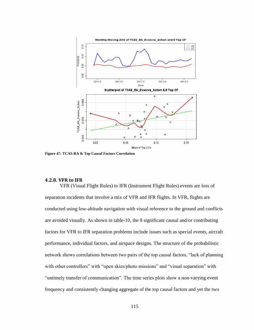
115
Figure 47: TCAS-RA & Top Causal Factors Correlation
4.2.8. VFR to IFR VFR (Visual Flight Rules) to IFR (Instrument Flight Rules) events are loss of
separation incidents that involve a mix of VFR and IFR flights. In VFR, flights are
conducted using low-altitude navigation with visual reference to the ground and conflicts
are avoided visually. As shown in table-10, the 8 significant causal and/or contributing
factors for VFR to IFR separation problems include issues such as special events, aircraft
performance, individual factors, and airspace designs. The structure of the probabilistic
network shows correlations between two pairs of the top causal factors, “lack of planning
with other controllers” with “open skies/photo missions” and “visual separation” with
“untimely transfer of communication”. The time series plots show a non-varying event
frequency and consistently changing aggregate of the top causal factors and yet the two
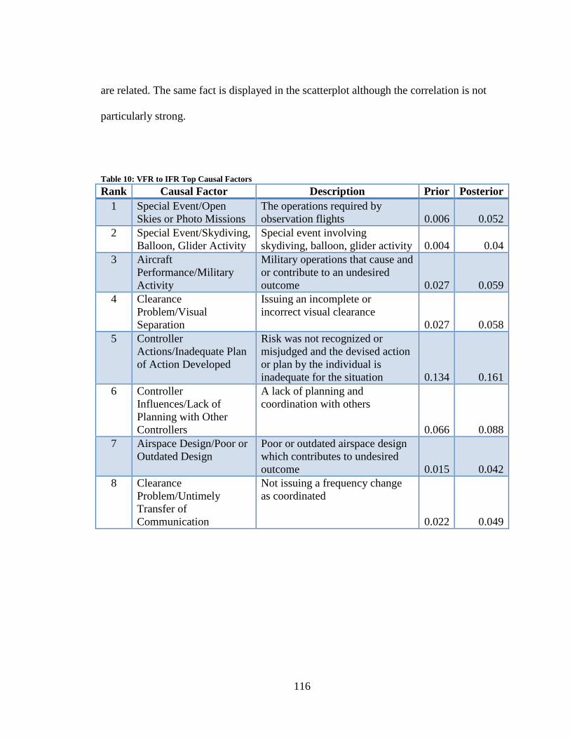
116
are related. The same fact is displayed in the scatterplot although the correlation is not
particularly strong.
Table 10: VFR to IFR Top Causal Factors
Rank Causal Factor Description Prior Posterior
1 Special Event/Open
Skies or Photo Missions
The operations required by
observation flights 0.006 0.052
2 Special Event/Skydiving,
Balloon, Glider Activity
Special event involving
skydiving, balloon, glider activity 0.004 0.04
3 Aircraft
Performance/Military
Activity
Military operations that cause and
or contribute to an undesired
outcome 0.027 0.059
4 Clearance
Problem/Visual
Separation
Issuing an incomplete or
incorrect visual clearance
0.027 0.058
5 Controller
Actions/Inadequate Plan
of Action Developed
Risk was not recognized or
misjudged and the devised action
or plan by the individual is
inadequate for the situation 0.134 0.161
6 Controller
Influences/Lack of
Planning with Other
Controllers
A lack of planning and
coordination with others
0.066 0.088
7 Airspace Design/Poor or
Outdated Design
Poor or outdated airspace design
which contributes to undesired
outcome 0.015 0.042
8 Clearance
Problem/Untimely
Transfer of
Communication
Not issuing a frequency change
as coordinated
0.022 0.049
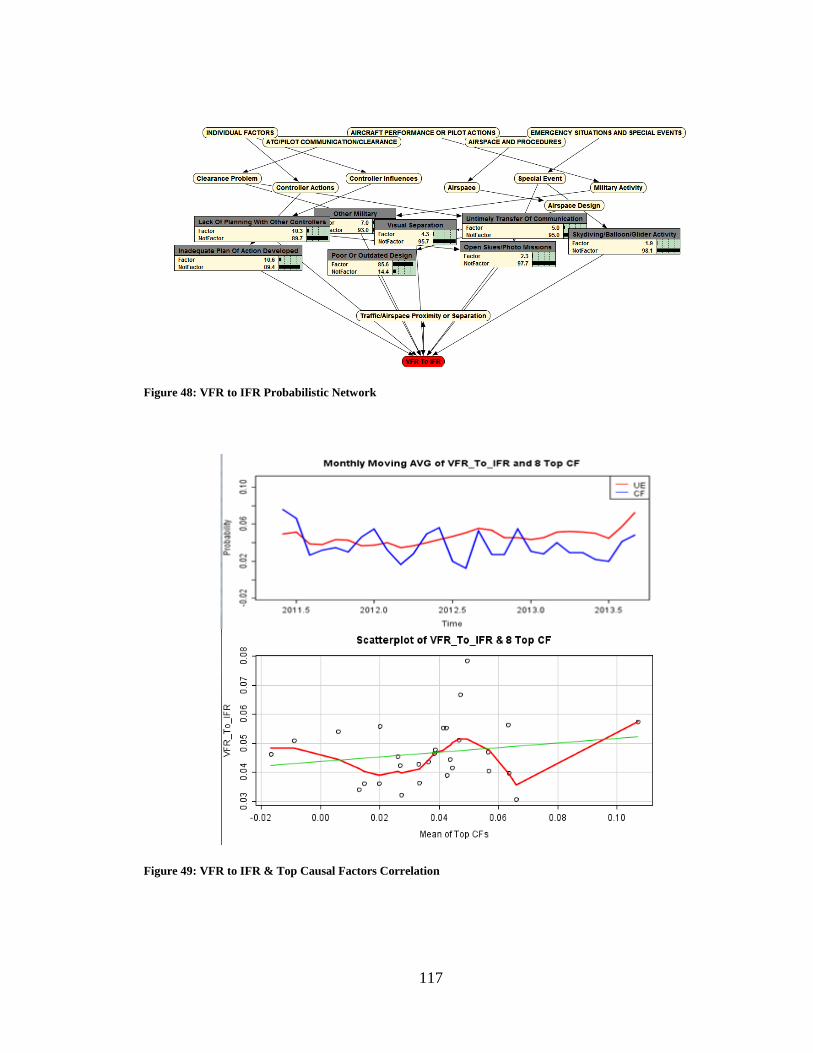
117
Figure 48: VFR to IFR Probabilistic Network
Figure 49: VFR to IFR & Top Causal Factors Correlation
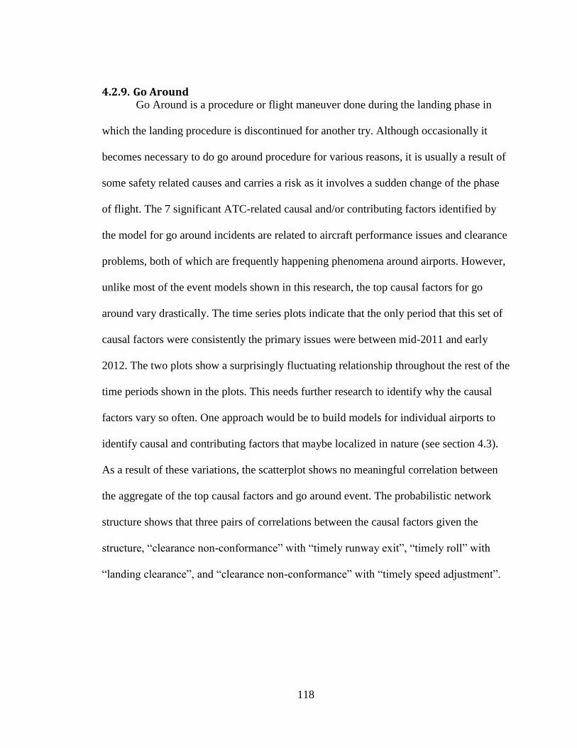
118
4.2.9. Go Around Go Around is a procedure or flight maneuver done during the landing phase in
which the landing procedure is discontinued for another try. Although occasionally it
becomes necessary to do go around procedure for various reasons, it is usually a result of
some safety related causes and carries a risk as it involves a sudden change of the phase
of flight. The 7 significant ATC-related causal and/or contributing factors identified by
the model for go around incidents are related to aircraft performance issues and clearance
problems, both of which are frequently happening phenomena around airports. However,
unlike most of the event models shown in this research, the top causal factors for go
around vary drastically. The time series plots indicate that the only period that this set of
causal factors were consistently the primary issues were between mid-2011 and early
2012. The two plots show a surprisingly fluctuating relationship throughout the rest of the
time periods shown in the plots. This needs further research to identify why the causal
factors vary so often. One approach would be to build models for individual airports to
identify causal and contributing factors that maybe localized in nature (see section 4.3).
As a result of these variations, the scatterplot shows no meaningful correlation between
the aggregate of the top causal factors and go around event. The probabilistic network
structure shows that three pairs of correlations between the causal factors given the
structure, “clearance non-conformance” with “timely runway exit”, “timely roll” with
“landing clearance”, and “clearance non-conformance” with “timely speed adjustment”.
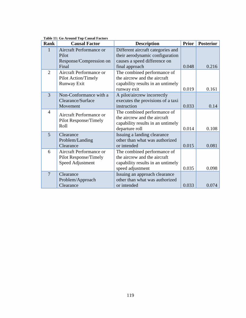
119
Table 11: Go Around Top Causal Factors
Rank Causal Factor Description Prior Posterior
1 Aircraft Performance or
Pilot
Response/Compression on
Final
Different aircraft categories and
their aerodynamic configuration
causes a speed difference on
final approach 0.048 0.216
2 Aircraft Performance or
Pilot Action/Timely
Runway Exit
The combined performance of
the aircrew and the aircraft
capability results in an untimely
runway exit 0.019 0.161
3 Non-Conformance with a
Clearance/Surface
Movement
A pilot/aircrew incorrectly
executes the provisions of a taxi
instruction 0.033 0.14
4 Aircraft Performance or
Pilot Response/Timely
Roll
The combined performance of
the aircrew and the aircraft
capability results in an untimely
departure roll 0.014 0.108
5 Clearance
Problem/Landing
Clearance
Issuing a landing clearance
other than what was authorized
or intended 0.015 0.081
6 Aircraft Performance or
Pilot Response/Timely
Speed Adjustment
The combined performance of
the aircrew and the aircraft
capability results in an untimely
speed adjustment 0.035 0.098
7 Clearance
Problem/Approach
Clearance
Issuing an approach clearance
other than what was authorized
or intended 0.033 0.074
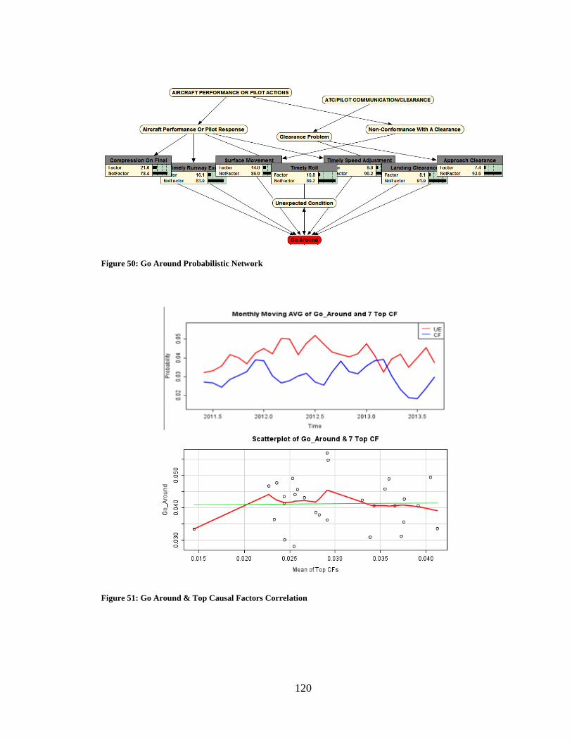
120
Figure 50: Go Around Probabilistic Network
Figure 51: Go Around & Top Causal Factors Correlation

121
4.2.10. Wake Turbulence Wake turbulence events are caused by the turbulence effects of one aircraft on
other aircraft nearby, usually behind, but also on those on parallel paths primarily during
landing and takeoff phases. The turbulence is created by the spillover of the air at the
wingtip due to the pressure differential between the lower and upper surface of the wing.
Depending on the strength of the turbulence, the separation distance, and size of the
affected aircraft, wake turbulence can lead to issues that range from minor instability to a
major aircraft roll. The 6 significant causal factors (see table-12) for turbulence incidents
identified in the model include issues like aircraft performance, pilot response, and
clearance problems. Pilot response is one of the top factors mainly because flight crews
are primarily responsible to operate aircraft in the optimal path for wake turbulence with
little assistance from ATC within the given clearance. The structure of the causal model
shows no correlation between any pair of the causal factors given the learned structure,
which implies that all the causal factors are independent of each other for wake
turbulence events. However, the time series plots and the scatterplot display a relatively
strong relationship between the aggregate of the top causal factors and wake turbulence
event frequency. Similarly, the strong correlation between the two parameters is shown in
the scatterplots.
Table 12: Wake Turbulence Top Causal Factors
Rank Causal Factor Description Prior Posterior
1 Aircraft Performance or
Pilot
Response/Compression
on Final
Different aircraft categories and
their aerodynamic configuration
causes a speed difference on
final approach 0.048 0.29
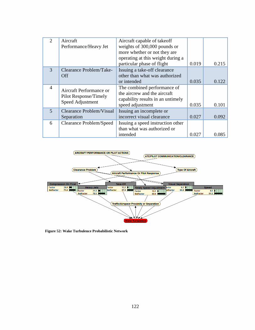
122
2 Aircraft
Performance/Heavy Jet
Aircraft capable of takeoff
weights of 300,000 pounds or
more whether or not they are
operating at this weight during a
particular phase of flight 0.019 0.215
3 Clearance Problem/Take-
Off
Issuing a take-off clearance
other than what was authorized
or intended 0.035 0.122
4 Aircraft Performance or
Pilot Response/Timely
Speed Adjustment
The combined performance of
the aircrew and the aircraft
capability results in an untimely
speed adjustment 0.035 0.101
5 Clearance Problem/Visual
Separation
Issuing an incomplete or
incorrect visual clearance 0.027 0.092
6 Clearance Problem/Speed Issuing a speed instruction other
than what was authorized or
intended 0.027 0.085
Figure 52: Wake Turbulence Probabilistic Network
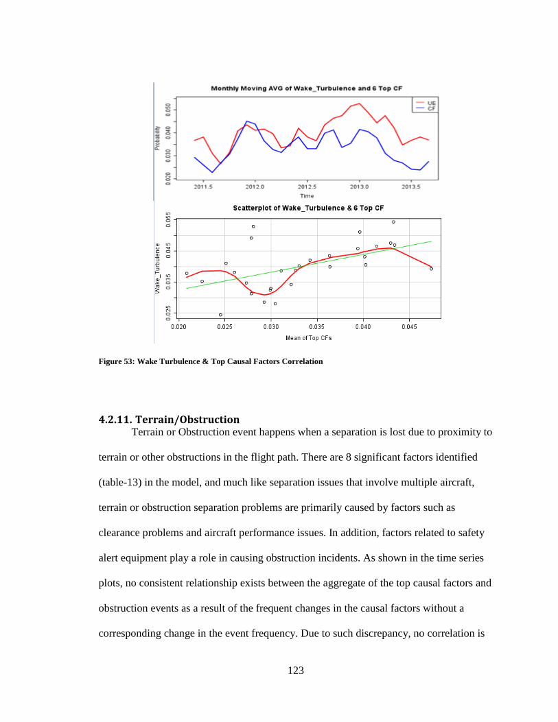
123
Figure 53: Wake Turbulence & Top Causal Factors Correlation
4.2.11. Terrain/Obstruction Terrain or Obstruction event happens when a separation is lost due to proximity to
terrain or other obstructions in the flight path. There are 8 significant factors identified
(table-13) in the model, and much like separation issues that involve multiple aircraft,
terrain or obstruction separation problems are primarily caused by factors such as
clearance problems and aircraft performance issues. In addition, factors related to safety
alert equipment play a role in causing obstruction incidents. As shown in the time series
plots, no consistent relationship exists between the aggregate of the top causal factors and
obstruction events as a result of the frequent changes in the causal factors without a
corresponding change in the event frequency. Due to such discrepancy, no correlation is
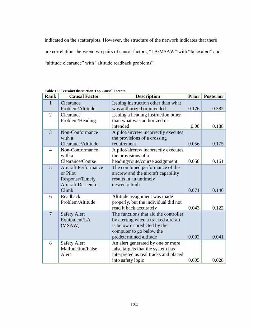
124
indicated on the scatterplots. However, the structure of the network indicates that there
are correlations between two pairs of causal factors, “LA/MSAW” with “false alert” and
“altitude clearance” with “altitude readback problems”.
Table 13: Terrain/Obstruction Top Causal Factors
Rank Causal Factor Description Prior Posterior
1 Clearance
Problem/Altitude
Issuing instruction other than what
was authorized or intended 0.176 0.382
2 Clearance
Problem/Heading
Issuing a heading instruction other
than what was authorized or
intended 0.08 0.188
3 Non-Conformance
with a
Clearance/Altitude
A pilot/aircrew incorrectly executes
the provisions of a crossing
requirement 0.056 0.175
4 Non-Conformance
with a
Clearance/Course
A pilot/aircrew incorrectly executes
the provisions of a
heading/route/course assignment 0.058 0.161
5 Aircraft Performance
or Pilot
Response/Timely
Aircraft Descent or
Climb
The combined performance of the
aircrew and the aircraft capability
results in an untimely
descent/climb
0.071 0.146
6 Readback
Problem/Altitude
Altitude assignment was made
properly, but the individual did not
read it back accurately 0.043 0.122
7 Safety Alert
Equipment/LA
(MSAW)
The functions that aid the controller
by alerting when a tracked aircraft
is below or predicted by the
computer to go below the
predetermined altitude 0.002 0.041
8 Safety Alert
Malfunction/False
Alert
An alert generated by one or more
false targets that the system has
interpreted as real tracks and placed
into safety logic 0.005 0.028
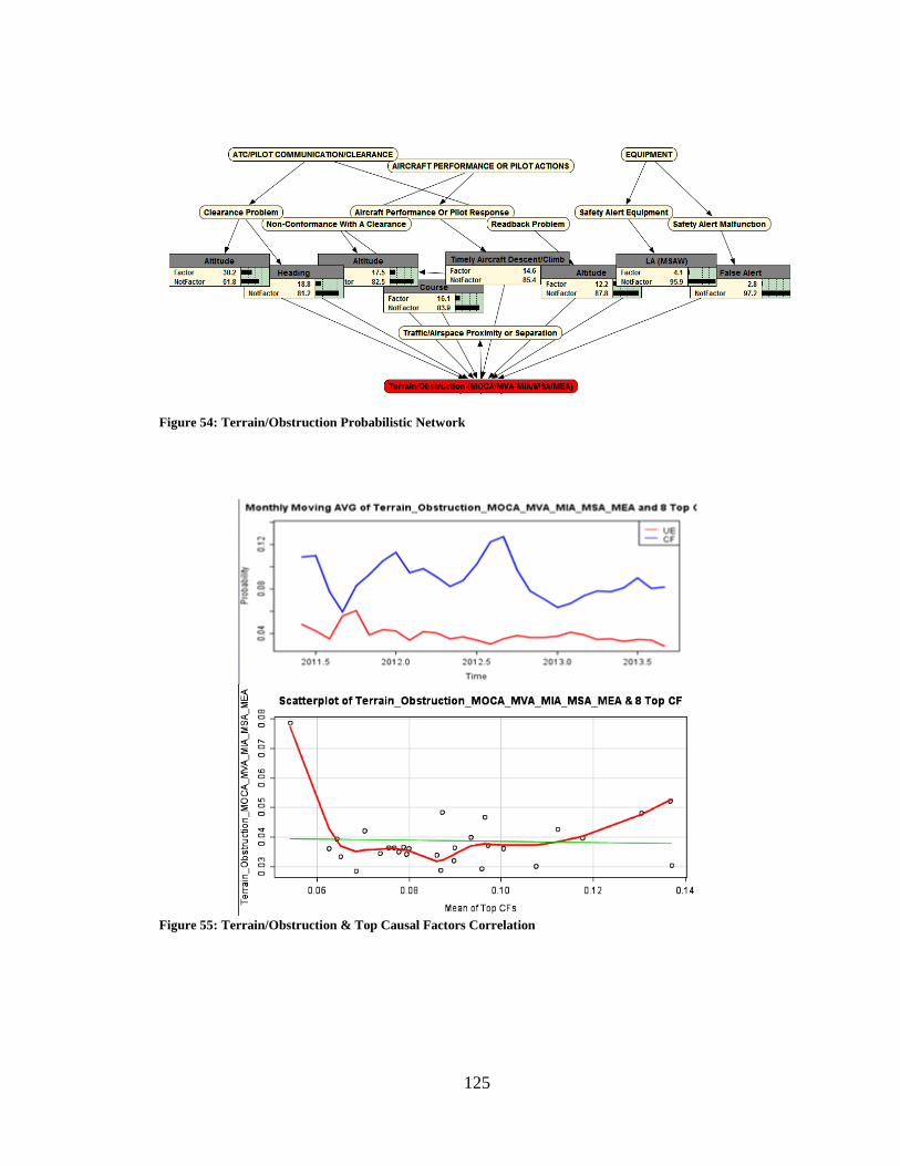
125
Figure 54: Terrain/Obstruction Probabilistic Network
Figure 55: Terrain/Obstruction & Top Causal Factors Correlation
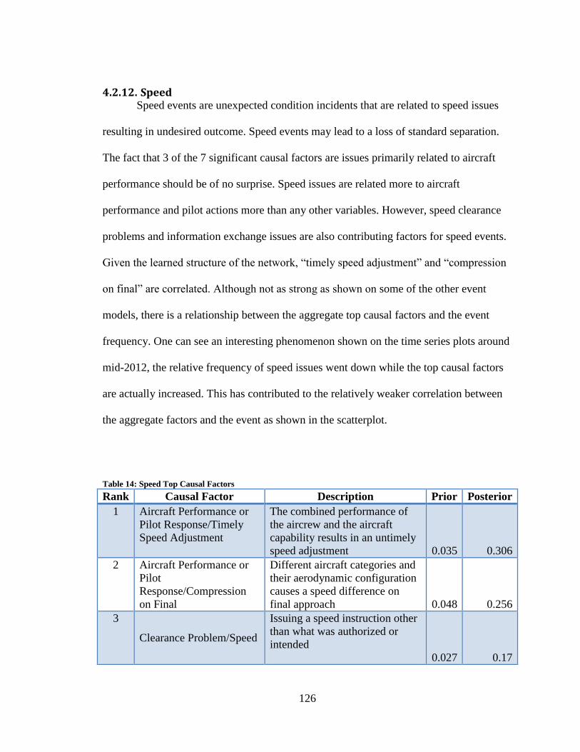
126
4.2.12. Speed Speed events are unexpected condition incidents that are related to speed issues
resulting in undesired outcome. Speed events may lead to a loss of standard separation.
The fact that 3 of the 7 significant causal factors are issues primarily related to aircraft
performance should be of no surprise. Speed issues are related more to aircraft
performance and pilot actions more than any other variables. However, speed clearance
problems and information exchange issues are also contributing factors for speed events.
Given the learned structure of the network, “timely speed adjustment” and “compression
on final” are correlated. Although not as strong as shown on some of the other event
models, there is a relationship between the aggregate top causal factors and the event
frequency. One can see an interesting phenomenon shown on the time series plots around
mid-2012, the relative frequency of speed issues went down while the top causal factors
are actually increased. This has contributed to the relatively weaker correlation between
the aggregate factors and the event as shown in the scatterplot.
Table 14: Speed Top Causal Factors
Rank Causal Factor Description Prior Posterior
1 Aircraft Performance or
Pilot Response/Timely
Speed Adjustment
The combined performance of
the aircrew and the aircraft
capability results in an untimely
speed adjustment 0.035 0.306
2 Aircraft Performance or
Pilot
Response/Compression
on Final
Different aircraft categories and
their aerodynamic configuration
causes a speed difference on
final approach 0.048 0.256
3
Clearance Problem/Speed
Issuing a speed instruction other
than what was authorized or
intended
0.027 0.17
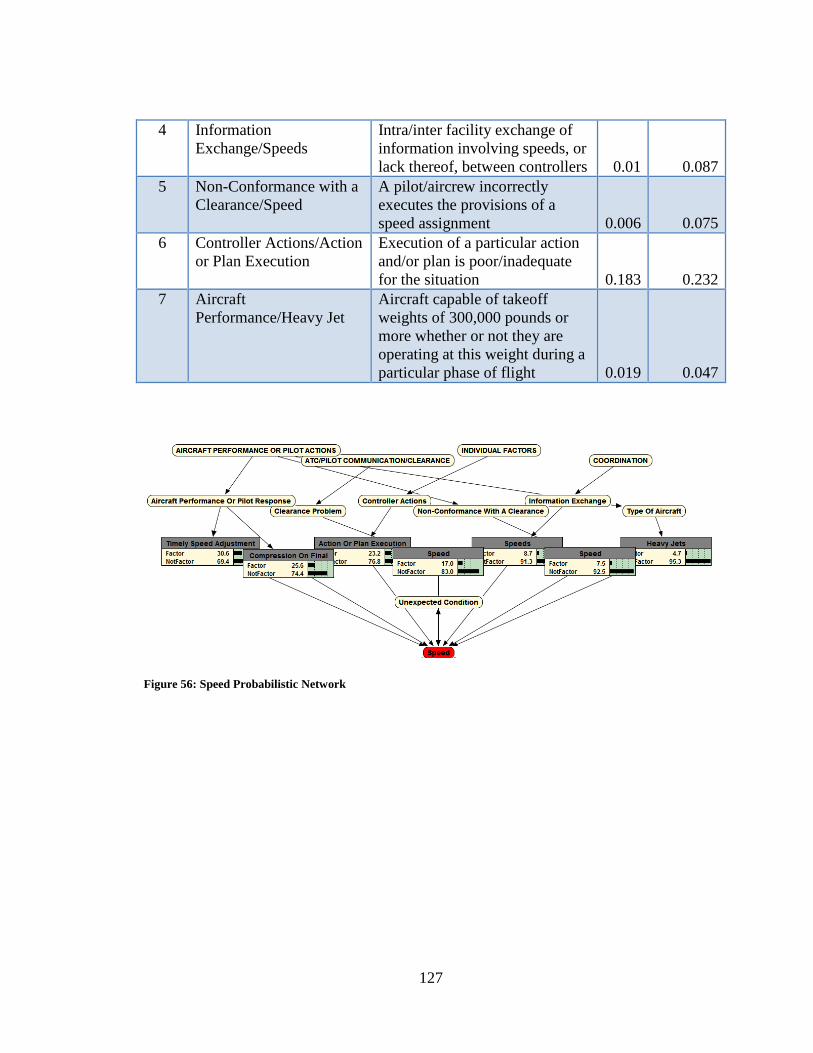
127
4 Information
Exchange/Speeds
Intra/inter facility exchange of
information involving speeds, or
lack thereof, between controllers 0.01 0.087
5 Non-Conformance with a
Clearance/Speed
A pilot/aircrew incorrectly
executes the provisions of a
speed assignment 0.006 0.075
6 Controller Actions/Action
or Plan Execution
Execution of a particular action
and/or plan is poor/inadequate
for the situation 0.183 0.232
7 Aircraft
Performance/Heavy Jet
Aircraft capable of takeoff
weights of 300,000 pounds or
more whether or not they are
operating at this weight during a
particular phase of flight 0.019 0.047
Figure 56: Speed Probabilistic Network
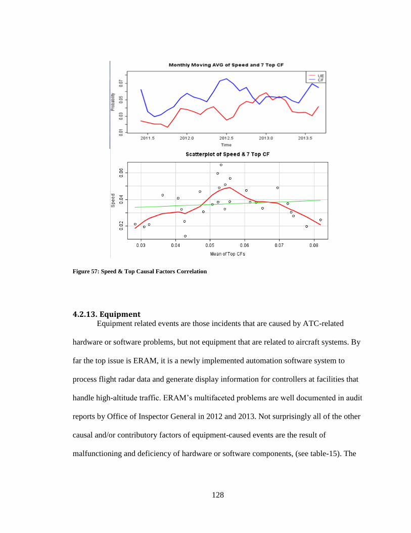
128
Figure 57: Speed & Top Causal Factors Correlation
4.2.13. Equipment Equipment related events are those incidents that are caused by ATC-related
hardware or software problems, but not equipment that are related to aircraft systems. By
far the top issue is ERAM, it is a newly implemented automation software system to
process flight radar data and generate display information for controllers at facilities that
handle high-altitude traffic. ERAM’s multifaceted problems are well documented in audit
reports by Office of Inspector General in 2012 and 2013. Not surprisingly all of the other
causal and/or contributory factors of equipment-caused events are the result of
malfunctioning and deficiency of hardware or software components, (see table-15). The
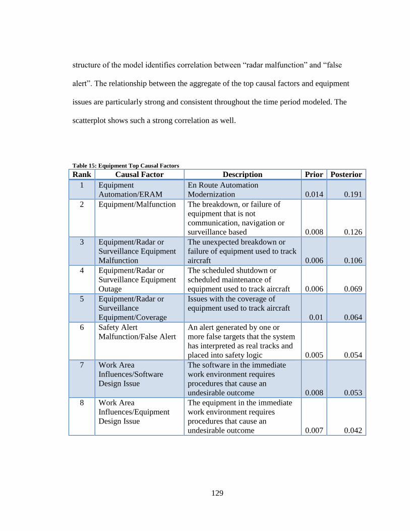
129
structure of the model identifies correlation between “radar malfunction” and “false
alert”. The relationship between the aggregate of the top causal factors and equipment
issues are particularly strong and consistent throughout the time period modeled. The
scatterplot shows such a strong correlation as well.
Table 15: Equipment Top Causal Factors
Rank Causal Factor Description Prior Posterior
1 Equipment
Automation/ERAM
En Route Automation
Modernization 0.014 0.191
2 Equipment/Malfunction The breakdown, or failure of
equipment that is not
communication, navigation or
surveillance based 0.008 0.126
3 Equipment/Radar or
Surveillance Equipment
Malfunction
The unexpected breakdown or
failure of equipment used to track
aircraft 0.006 0.106
4 Equipment/Radar or
Surveillance Equipment
Outage
The scheduled shutdown or
scheduled maintenance of
equipment used to track aircraft 0.006 0.069
5 Equipment/Radar or
Surveillance
Equipment/Coverage
Issues with the coverage of
equipment used to track aircraft
0.01 0.064
6 Safety Alert
Malfunction/False Alert
An alert generated by one or
more false targets that the system
has interpreted as real tracks and
placed into safety logic 0.005 0.054
7 Work Area
Influences/Software
Design Issue
The software in the immediate
work environment requires
procedures that cause an
undesirable outcome 0.008 0.053
8 Work Area
Influences/Equipment
Design Issue
The equipment in the immediate
work environment requires
procedures that cause an
undesirable outcome 0.007 0.042
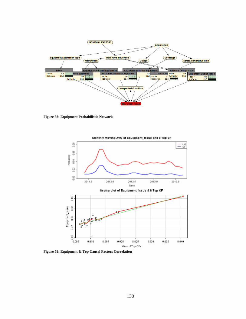
130
Figure 58: Equipment Probabilistic Network
Figure 59: Equipment & Top Causal Factors Correlation
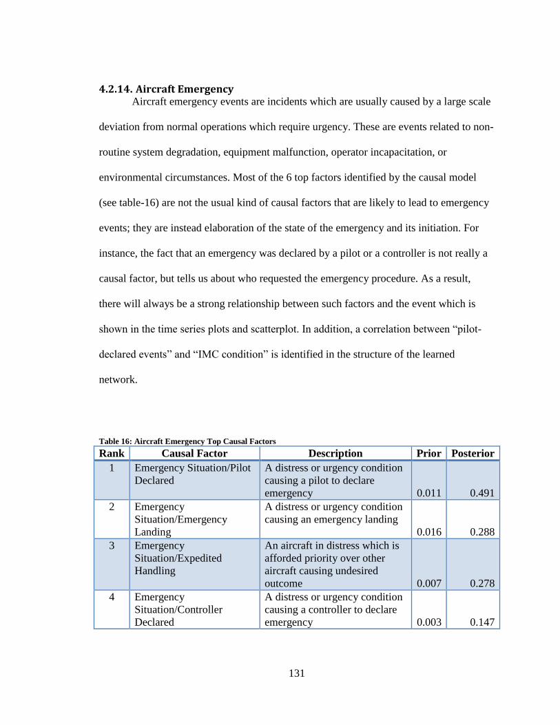
131
4.2.14. Aircraft Emergency Aircraft emergency events are incidents which are usually caused by a large scale
deviation from normal operations which require urgency. These are events related to non-
routine system degradation, equipment malfunction, operator incapacitation, or
environmental circumstances. Most of the 6 top factors identified by the causal model
(see table-16) are not the usual kind of causal factors that are likely to lead to emergency
events; they are instead elaboration of the state of the emergency and its initiation. For
instance, the fact that an emergency was declared by a pilot or a controller is not really a
causal factor, but tells us about who requested the emergency procedure. As a result,
there will always be a strong relationship between such factors and the event which is
shown in the time series plots and scatterplot. In addition, a correlation between “pilot-
declared events” and “IMC condition” is identified in the structure of the learned
network.
Table 16: Aircraft Emergency Top Causal Factors
Rank Causal Factor Description Prior Posterior
1 Emergency Situation/Pilot
Declared
A distress or urgency condition
causing a pilot to declare
emergency 0.011 0.491
2 Emergency
Situation/Emergency
Landing
A distress or urgency condition
causing an emergency landing
0.016 0.288
3 Emergency
Situation/Expedited
Handling
An aircraft in distress which is
afforded priority over other
aircraft causing undesired
outcome 0.007 0.278
4 Emergency
Situation/Controller
Declared
A distress or urgency condition
causing a controller to declare
emergency 0.003 0.147
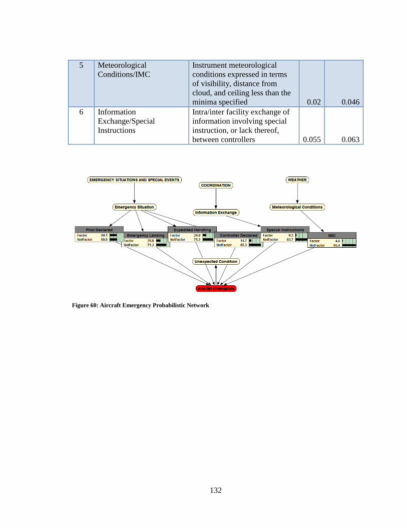
132
5 Meteorological
Conditions/IMC
Instrument meteorological
conditions expressed in terms
of visibility, distance from
cloud, and ceiling less than the
minima specified 0.02 0.046
6 Information
Exchange/Special
Instructions
Intra/inter facility exchange of
information involving special
instruction, or lack thereof,
between controllers 0.055 0.063
Figure 60: Aircraft Emergency Probabilistic Network
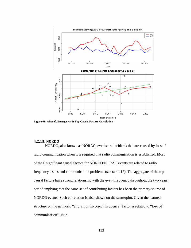
133
Figure 61: Aircraft Emergency & Top Causal Factors Correlation
4.2.15. NORDO NORDO, also known as NORAC, events are incidents that are caused by loss of
radio communication when it is required that radio communication is established. Most
of the 6 significant causal factors for NORDO/NORAC events are related to radio
frequency issues and communication problems (see table-17). The aggregate of the top
causal factors have strong relationship with the event frequency throughout the two years
period implying that the same set of contributing factors has been the primary source of
NORDO events. Such correlation is also shown on the scatterplot. Given the learned
structure on the network, “aircraft on incorrect frequency” factor is related to “lose of
communication” issue.
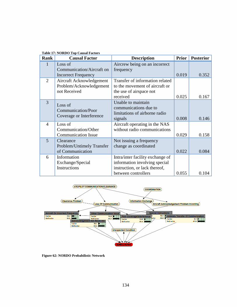
134
Table 17: NORDO Top Causal Factors
Rank Causal Factor Description Prior Posterior
1 Loss of
Communication/Aircraft on
Incorrect Frequency
Aircrew being on an incorrect
frequency
0.019 0.352
2 Aircraft Acknowledgement
Problem/Acknowledgement
not Received
Transfer of information related
to the movement of aircraft or
the use of airspace not
received 0.025 0.167
3 Loss of
Communication/Poor
Coverage or Interference
Unable to maintain
communications due to
limitations of airborne radio
signals 0.008 0.146
4 Loss of
Communication/Other
Communication Issue
Aircraft operating in the NAS
without radio communications
0.029 0.158
5 Clearance
Problem/Untimely Transfer
of Communication
Not issuing a frequency
change as coordinated
0.022 0.084
6 Information
Exchange/Special
Instructions
Intra/inter facility exchange of
information involving special
instruction, or lack thereof,
between controllers 0.055 0.104
Figure 62: NORDO Probabilistic Network
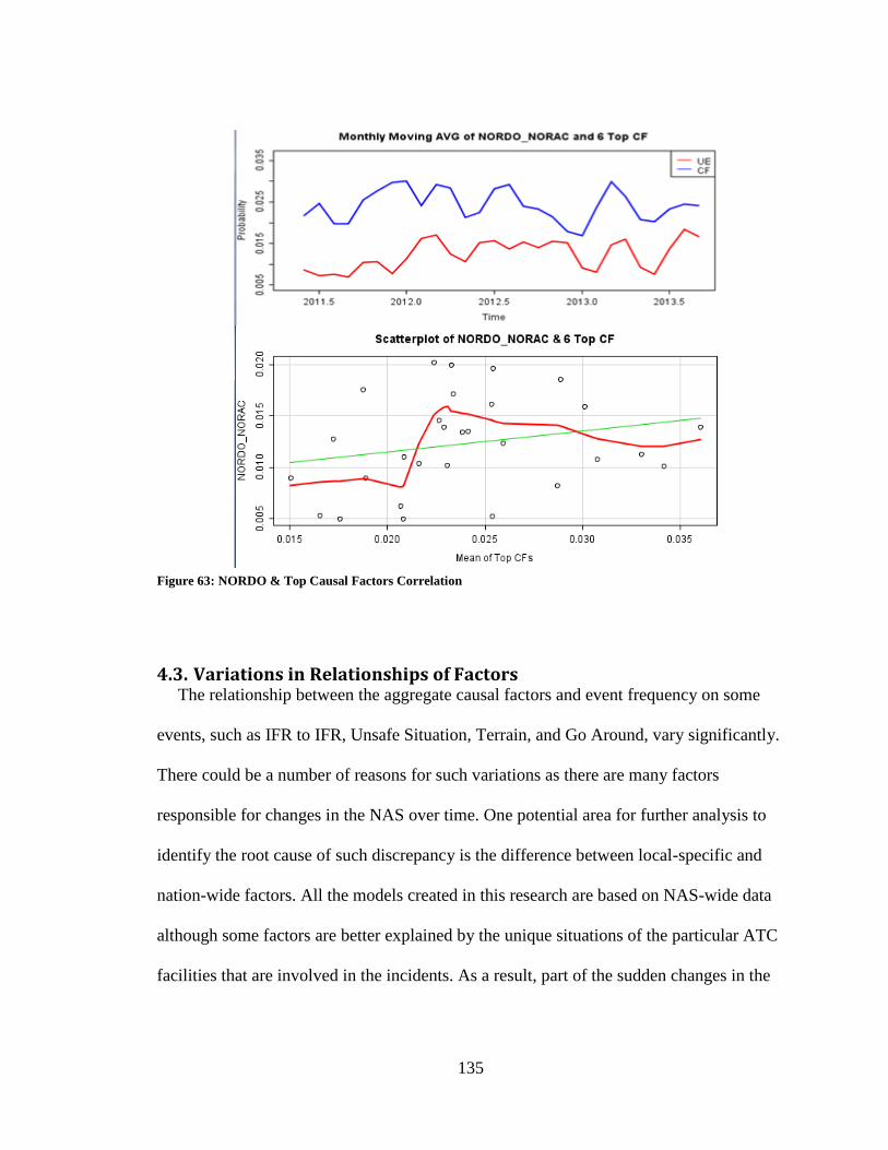
135
Figure 63: NORDO & Top Causal Factors Correlation
4.3. Variations in Relationships of Factors The relationship between the aggregate causal factors and event frequency on some
events, such as IFR to IFR, Unsafe Situation, Terrain, and Go Around, vary significantly.
There could be a number of reasons for such variations as there are many factors
responsible for changes in the NAS over time. One potential area for further analysis to
identify the root cause of such discrepancy is the difference between local-specific and
nation-wide factors. All the models created in this research are based on NAS-wide data
although some factors are better explained by the unique situations of the particular ATC
facilities that are involved in the incidents. As a result, part of the sudden changes in the
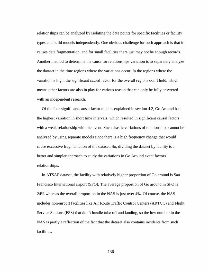
136
relationships can be analyzed by isolating the data points for specific facilities or facility
types and build models independently. One obvious challenge for such approach is that it
causes data fragmentation, and for small facilities there just may not be enough records.
Another method to determine the cause for relationships variation is to separately analyze
the dataset in the time regions where the variations occur. In the regions where the
variation is high, the significant causal factor for the overall regions don’t hold, which
means other factors are also in play for various reason that can only be fully answered
with an independent research.
Of the four significant causal factor models explained in section 4.2, Go Around has
the highest variation in short time intervals, which resulted in significant causal factors
with a weak relationship with the event. Such drastic variations of relationships cannot be
analyzed by using separate models since there is a high frequency change that would
cause excessive fragmentation of the dataset. So, dividing the dataset by facility is a
better and simpler approach to study the variations in Go Around event factors
relationships.
In ATSAP dataset, the facility with relatively higher proportion of Go around is San
Francisco International airport (SFO). The average proportion of Go around in SFO is
24% whereas the overall proportion in the NAS is just over 4%. Of course, the NAS
includes non-airport facilities like Air Route Traffic Control Centers (ARTCC) and Flight
Service Stations (FSS) that don’t handle take-off and landing, so the low number in the
NAS is partly a reflection of the fact that the dataset also contains incidents from such
facilities.
137
The probabilistic causal model shown below in figure-64 identifies three new causal
factors that were not part of the Go Around event in the NAS model. The SFO causal
model identifies a total of 8 causal factors as significant for Go Around of which only 4
matches with the model for the NAS (the NAS model has only 6 factors). The two new
causal factors, “unwritten facility practices” and “poor or outdated design” are specific to
the facility and the airspace it serves. Also “event inconsistence with experience” factor
could be unique to the facility. A clearance problem involving surface movement which
is one of the top issues in the NAS model is not identified as a causal factor for the SFO
local model. The interesting result of this model is that unlike the NAS model, there is a
significant relationship between the causal factors and the event frequency throughout the
two year period (see figure-65).
Figure 64: Go Around Probabilistic Network for SFO Facility
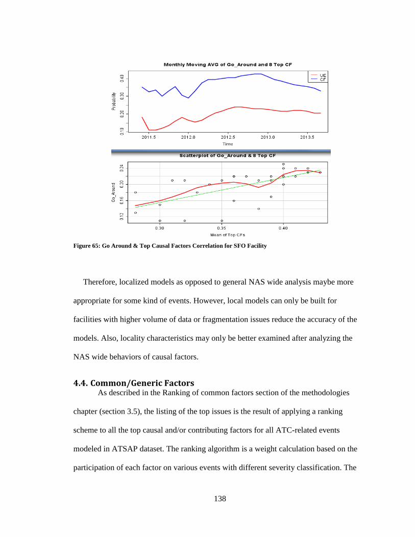
138
Figure 65: Go Around & Top Causal Factors Correlation for SFO Facility
Therefore, localized models as opposed to general NAS wide analysis maybe more
appropriate for some kind of events. However, local models can only be built for
facilities with higher volume of data or fragmentation issues reduce the accuracy of the
models. Also, locality characteristics may only be better examined after analyzing the
NAS wide behaviors of causal factors.
4.4. Common/Generic Factors As described in the Ranking of common factors section of the methodologies
chapter (section 3.5), the listing of the top issues is the result of applying a ranking
scheme to all the top causal and/or contributing factors for all ATC-related events
modeled in ATSAP dataset. The ranking algorithm is a weight calculation based on the
participation of each factor on various events with different severity classification. The
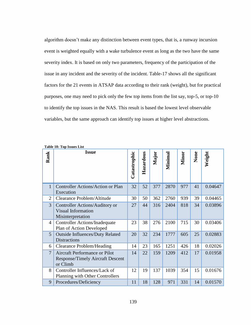
139
algorithm doesn’t make any distinction between event types, that is, a runway incursion
event is weighted equally with a wake turbulence event as long as the two have the same
severity index. It is based on only two parameters, frequency of the participation of the
issue in any incident and the severity of the incident. Table-17 shows all the significant
factors for the 21 events in ATSAP data according to their rank (weight), but for practical
purposes, one may need to pick only the few top items from the list say, top-5, or top-10
to identify the top issues in the NAS. This result is based the lowest level observable
variables, but the same approach can identify top issues at higher level abstractions.
Table 18: Top Issues List
Ran
k
Issue
Cata
stro
ph
ic
Haza
rdou
s
Majo
r
Min
imal
Min
or
Non
e
Wei
gh
t
1 Controller Actions/Action or Plan
Execution
32 52 377 2870 977 41 0.04647
2 Clearance Problem/Altitude 30 50 362 2760 939 39 0.04465
3 Controller Actions/Auditory or
Visual Information
Misinterpretation
27 44 316 2404 818 34 0.03896
4 Controller Actions/Inadequate
Plan of Action Developed
23 38 276 2100 715 30 0.03406
5 Outside Influences/Duty Related
Distractions
20 32 234 1777 605 25 0.02883
6 Clearance Problem/Heading 14 23 165 1251 426 18 0.02026
7 Aircraft Performance or Pilot
Response/Timely Aircraft Descent
or Climb
14 22 159 1209 412 17 0.01958
8 Controller Influences/Lack of
Planning with Other Controllers
12 19 137 1039 354 15 0.01676
9 Procedures/Deficiency 11 18 128 971 331 14 0.01570
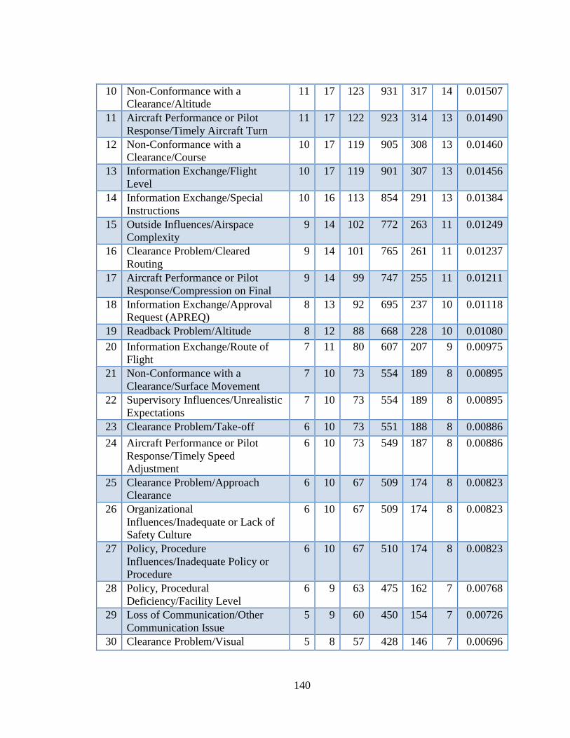
140
10 Non-Conformance with a
Clearance/Altitude
11 17 123 931 317 14 0.01507
11 Aircraft Performance or Pilot
Response/Timely Aircraft Turn
11 17 122 923 314 13 0.01490
12 Non-Conformance with a
Clearance/Course
10 17 119 905 308 13 0.01460
13 Information Exchange/Flight
Level
10 17 119 901 307 13 0.01456
14 Information Exchange/Special
Instructions
10 16 113 854 291 13 0.01384
15 Outside Influences/Airspace
Complexity
9 14 102 772 263 11 0.01249
16 Clearance Problem/Cleared
Routing
9 14 101 765 261 11 0.01237
17 Aircraft Performance or Pilot
Response/Compression on Final
9 14 99 747 255 11 0.01211
18 Information Exchange/Approval
Request (APREQ)
8 13 92 695 237 10 0.01118
19 Readback Problem/Altitude 8 12 88 668 228 10 0.01080
20 Information Exchange/Route of
Flight
7 11 80 607 207 9 0.00975
21 Non-Conformance with a
Clearance/Surface Movement
7 10 73 554 189 8 0.00895
22 Supervisory Influences/Unrealistic
Expectations
7 10 73 554 189 8 0.00895
23 Clearance Problem/Take-off 6 10 73 551 188 8 0.00886
24 Aircraft Performance or Pilot
Response/Timely Speed
Adjustment
6 10 73 549 187 8 0.00886
25 Clearance Problem/Approach
Clearance
6 10 67 509 174 8 0.00823
26 Organizational
Influences/Inadequate or Lack of
Safety Culture
6 10 67 509 174 8 0.00823
27 Policy, Procedure
Influences/Inadequate Policy or
Procedure
6 10 67 510 174 8 0.00823
28 Policy, Procedural
Deficiency/Facility Level
6 9 63 475 162 7 0.00768
29 Loss of Communication/Other
Communication Issue
5 9 60 450 154 7 0.00726
30 Clearance Problem/Visual 5 8 57 428 146 7 0.00696
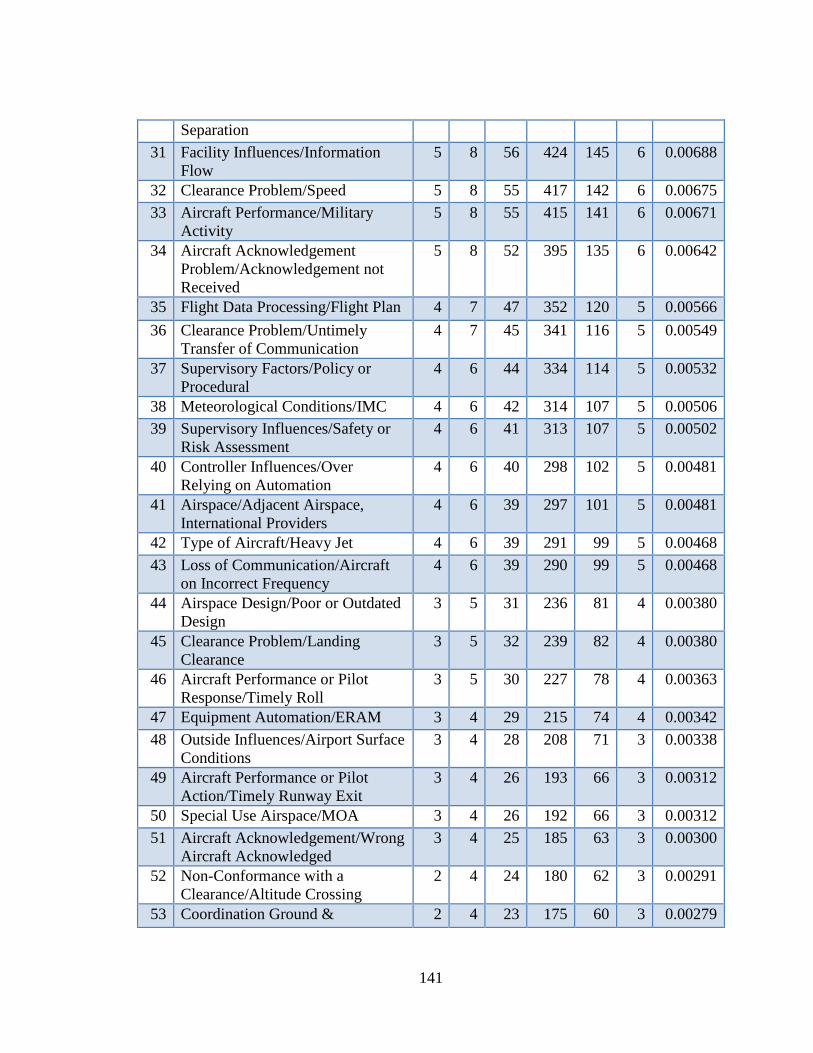
141
Separation
31 Facility Influences/Information
Flow
5 8 56 424 145 6 0.00688
32 Clearance Problem/Speed 5 8 55 417 142 6 0.00675
33 Aircraft Performance/Military
Activity
5 8 55 415 141 6 0.00671
34 Aircraft Acknowledgement
Problem/Acknowledgement not
Received
5 8 52 395 135 6 0.00642
35 Flight Data Processing/Flight Plan 4 7 47 352 120 5 0.00566
36 Clearance Problem/Untimely
Transfer of Communication
4 7 45 341 116 5 0.00549
37 Supervisory Factors/Policy or
Procedural
4 6 44 334 114 5 0.00532
38 Meteorological Conditions/IMC 4 6 42 314 107 5 0.00506
39 Supervisory Influences/Safety or
Risk Assessment
4 6 41 313 107 5 0.00502
40 Controller Influences/Over
Relying on Automation
4 6 40 298 102 5 0.00481
41 Airspace/Adjacent Airspace,
International Providers
4 6 39 297 101 5 0.00481
42 Type of Aircraft/Heavy Jet 4 6 39 291 99 5 0.00468
43 Loss of Communication/Aircraft
on Incorrect Frequency
4 6 39 290 99 5 0.00468
44 Airspace Design/Poor or Outdated
Design
3 5 31 236 81 4 0.00380
45 Clearance Problem/Landing
Clearance
3 5 32 239 82 4 0.00380
46 Aircraft Performance or Pilot
Response/Timely Roll
3 5 30 227 78 4 0.00363
47 Equipment Automation/ERAM 3 4 29 215 74 4 0.00342
48 Outside Influences/Airport Surface
Conditions
3 4 28 208 71 3 0.00338
49 Aircraft Performance or Pilot
Action/Timely Runway Exit
3 4 26 193 66 3 0.00312
50 Special Use Airspace/MOA 3 4 26 192 66 3 0.00312
51 Aircraft Acknowledgement/Wrong
Aircraft Acknowledged
3 4 25 185 63 3 0.00300
52 Non-Conformance with a
Clearance/Altitude Crossing
2 4 24 180 62 3 0.00291
53 Coordination Ground & 2 4 23 175 60 3 0.00279
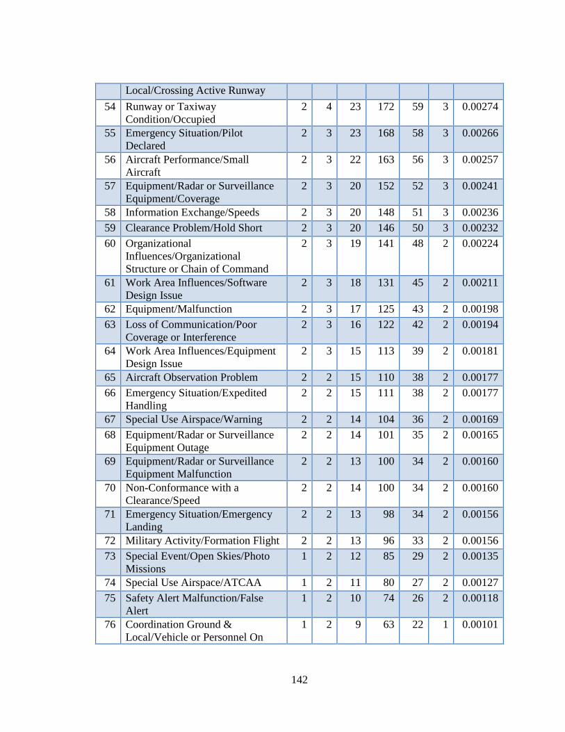
142
Local/Crossing Active Runway
54 Runway or Taxiway
Condition/Occupied
2 4 23 172 59 3 0.00274
55 Emergency Situation/Pilot
Declared
2 3 23 168 58 3 0.00266
56 Aircraft Performance/Small
Aircraft
2 3 22 163 56 3 0.00257
57 Equipment/Radar or Surveillance
Equipment/Coverage
2 3 20 152 52 3 0.00241
58 Information Exchange/Speeds 2 3 20 148 51 3 0.00236
59 Clearance Problem/Hold Short 2 3 20 146 50 3 0.00232
60 Organizational
Influences/Organizational
Structure or Chain of Command
2 3 19 141 48 2 0.00224
61 Work Area Influences/Software
Design Issue
2 3 18 131 45 2 0.00211
62 Equipment/Malfunction 2 3 17 125 43 2 0.00198
63 Loss of Communication/Poor
Coverage or Interference
2 3 16 122 42 2 0.00194
64 Work Area Influences/Equipment
Design Issue
2 3 15 113 39 2 0.00181
65 Aircraft Observation Problem 2 2 15 110 38 2 0.00177
66 Emergency Situation/Expedited
Handling
2 2 15 111 38 2 0.00177
67 Special Use Airspace/Warning 2 2 14 104 36 2 0.00169
68 Equipment/Radar or Surveillance
Equipment Outage
2 2 14 101 35 2 0.00165
69 Equipment/Radar or Surveillance
Equipment Malfunction
2 2 13 100 34 2 0.00160
70 Non-Conformance with a
Clearance/Speed
2 2 14 100 34 2 0.00160
71 Emergency Situation/Emergency
Landing
2 2 13 98 34 2 0.00156
72 Military Activity/Formation Flight 2 2 13 96 33 2 0.00156
73 Special Event/Open Skies/Photo
Missions
1 2 12 85 29 2 0.00135
74 Special Use Airspace/ATCAA 1 2 11 80 27 2 0.00127
75 Safety Alert Malfunction/False
Alert
1 2 10 74 26 2 0.00118
76 Coordination Ground &
Local/Vehicle or Personnel On
1 2 9 63 22 1 0.00101
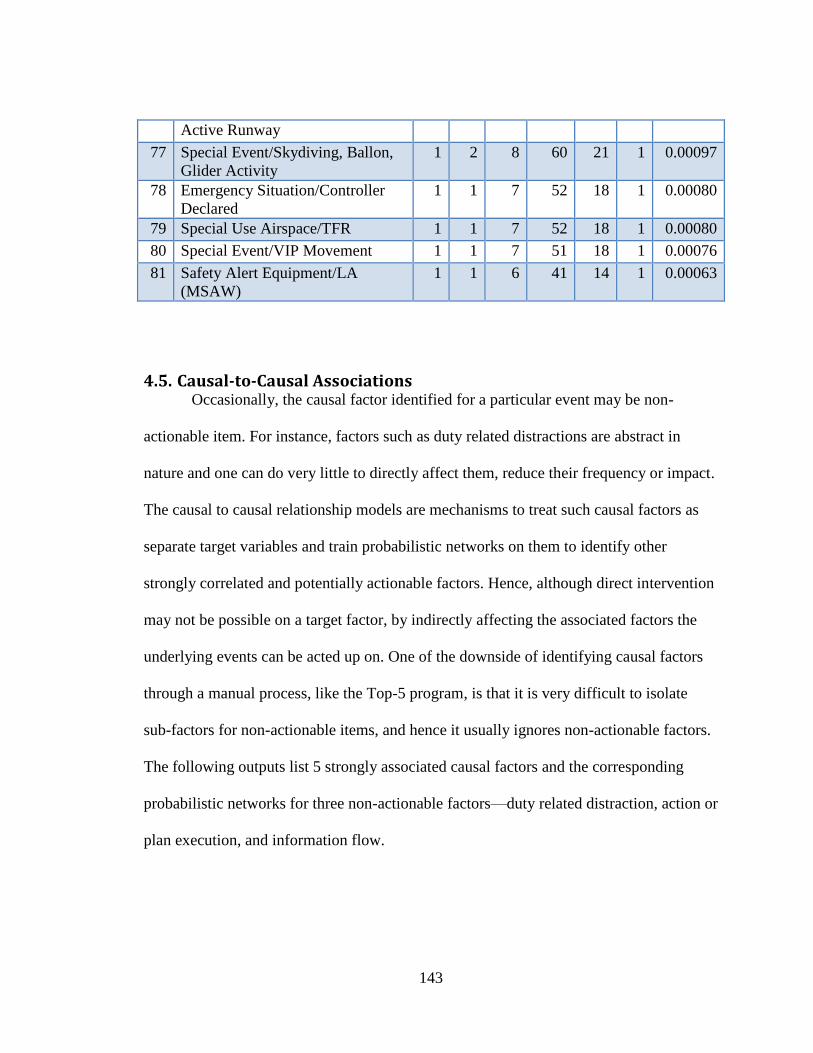
143
Active Runway
77 Special Event/Skydiving, Ballon,
Glider Activity
1 2 8 60 21 1 0.00097
78 Emergency Situation/Controller
Declared
1 1 7 52 18 1 0.00080
79 Special Use Airspace/TFR 1 1 7 52 18 1 0.00080
80 Special Event/VIP Movement 1 1 7 51 18 1 0.00076
81 Safety Alert Equipment/LA
(MSAW)
1 1 6 41 14 1 0.00063
4.5. Causal-to-Causal Associations Occasionally, the causal factor identified for a particular event may be non-
actionable item. For instance, factors such as duty related distractions are abstract in
nature and one can do very little to directly affect them, reduce their frequency or impact.
The causal to causal relationship models are mechanisms to treat such causal factors as
separate target variables and train probabilistic networks on them to identify other
strongly correlated and potentially actionable factors. Hence, although direct intervention
may not be possible on a target factor, by indirectly affecting the associated factors the
underlying events can be acted up on. One of the downside of identifying causal factors
through a manual process, like the Top-5 program, is that it is very difficult to isolate
sub-factors for non-actionable items, and hence it usually ignores non-actionable factors.
The following outputs list 5 strongly associated causal factors and the corresponding
probabilistic networks for three non-actionable factors—duty related distraction, action or
plan execution, and information flow.
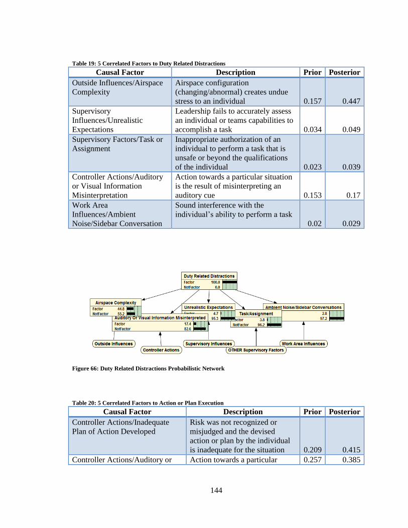
144
Table 19: 5 Correlated Factors to Duty Related Distractions
Causal Factor Description Prior Posterior
Outside Influences/Airspace
Complexity
Airspace configuration
(changing/abnormal) creates undue
stress to an individual 0.157 0.447
Supervisory
Influences/Unrealistic
Expectations
Leadership fails to accurately assess
an individual or teams capabilities to
accomplish a task 0.034 0.049
Supervisory Factors/Task or
Assignment
Inappropriate authorization of an
individual to perform a task that is
unsafe or beyond the qualifications
of the individual 0.023 0.039
Controller Actions/Auditory
or Visual Information
Misinterpretation
Action towards a particular situation
is the result of misinterpreting an
auditory cue 0.153 0.17
Work Area
Influences/Ambient
Noise/Sidebar Conversation
Sound interference with the
individual’s ability to perform a task
0.02 0.029
Figure 66: Duty Related Distractions Probabilistic Network
Table 20: 5 Correlated Factors to Action or Plan Execution
Causal Factor Description Prior Posterior
Controller Actions/Inadequate
Plan of Action Developed
Risk was not recognized or
misjudged and the devised
action or plan by the individual
is inadequate for the situation 0.209 0.415
Controller Actions/Auditory or Action towards a particular 0.257 0.385
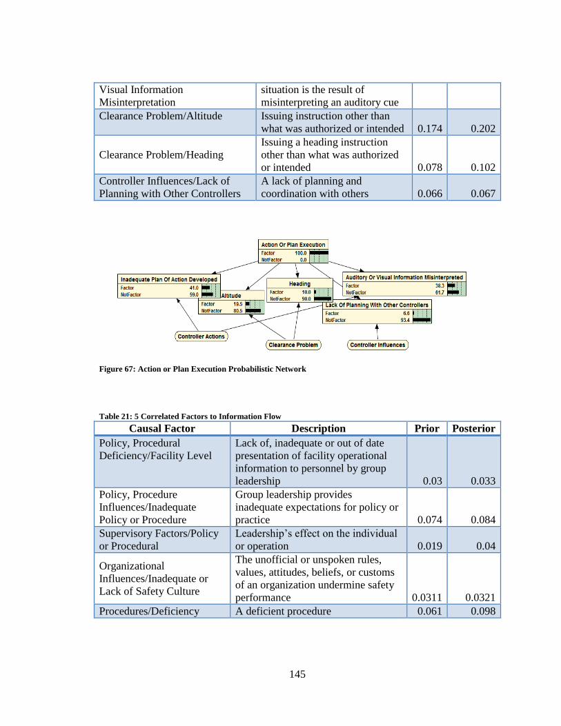
145
Visual Information
Misinterpretation
situation is the result of
misinterpreting an auditory cue
Clearance Problem/Altitude Issuing instruction other than
what was authorized or intended 0.174 0.202
Clearance Problem/Heading
Issuing a heading instruction
other than what was authorized
or intended 0.078 0.102
Controller Influences/Lack of
Planning with Other Controllers
A lack of planning and
coordination with others 0.066 0.067
Figure 67: Action or Plan Execution Probabilistic Network
Table 21: 5 Correlated Factors to Information Flow
Causal Factor Description Prior Posterior
Policy, Procedural
Deficiency/Facility Level
Lack of, inadequate or out of date
presentation of facility operational
information to personnel by group
leadership 0.03 0.033
Policy, Procedure
Influences/Inadequate
Policy or Procedure
Group leadership provides
inadequate expectations for policy or
practice 0.074 0.084
Supervisory Factors/Policy
or Procedural
Leadership’s effect on the individual
or operation 0.019 0.04
Organizational
Influences/Inadequate or
Lack of Safety Culture
The unofficial or unspoken rules,
values, attitudes, beliefs, or customs
of an organization undermine safety
performance 0.0311 0.0321
Procedures/Deficiency A deficient procedure 0.061 0.098
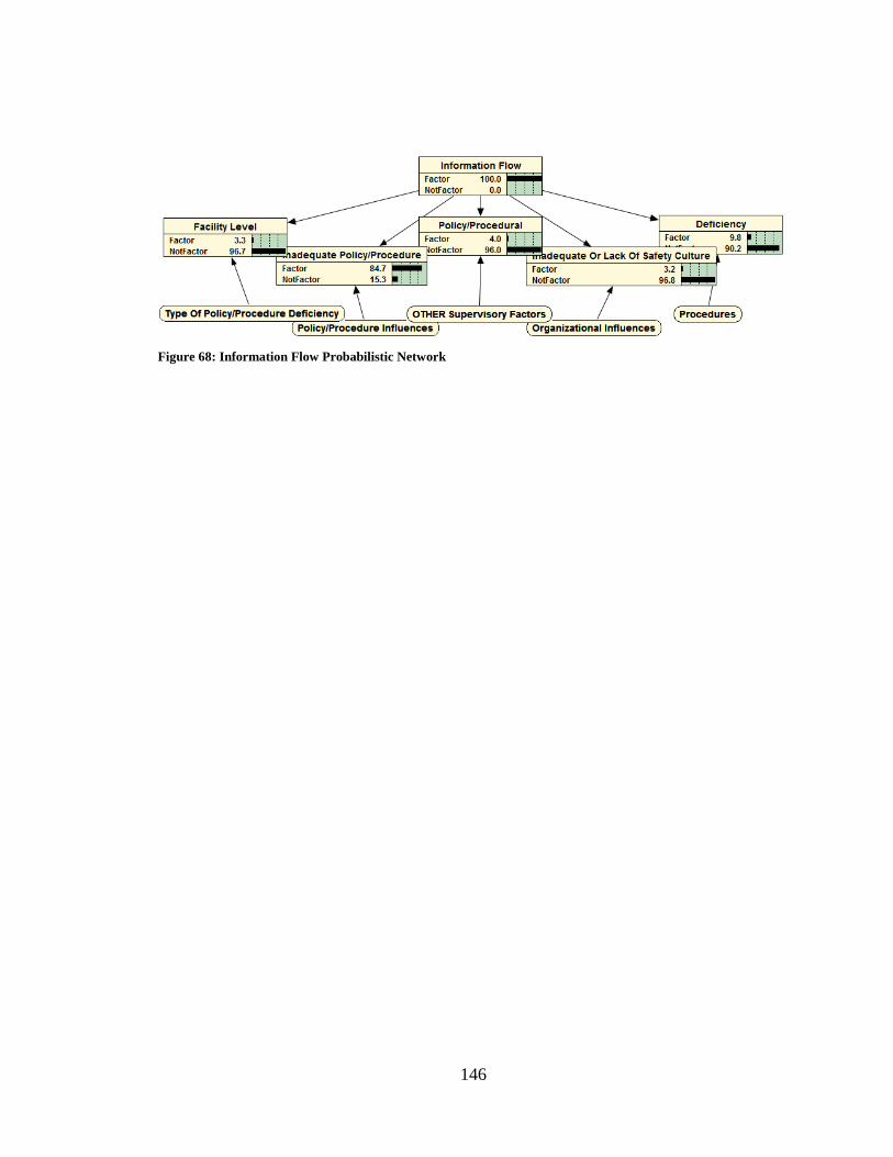
146
Figure 68: Information Flow Probabilistic Network
147
5. CONCLUSIONS
This chapter summarizes the background of the problem, the approaches used to
deal with the problem, and the research result. The research is primarily focused on the
study of ATC-related aviation events and their causal factors based on data from FAA’s
Air Traffic Safety Action Program (ATSAP). The core of the research is identifying
significant causal factors for each event type from a large number of factors using a
combination of exiting methodologies and others introduced in this dissertation.
5.1. Two-Phased Factor Selection The algorithm used to identify the causal factors is a generic method that can be
applied in any problem domain with the need to select small number of relevant
variables. The purpose of the selection of fewer variables may be for increasing the
performance of the target prediction or simplifying the problem by reducing the
dimension. One example of such problems is the identification of most relevant factors to
diagnose a disease. Unlike analyses that are based on simple frequency counts, this
research applies the difference of prior and posterior probabilities to measure the impact
of causal factors on individual events. The causal factor identification process follows a
two-phased approach. In the first phase, sensitivity analysis is conducted using the
difference of prior and posterior probabilities of each causal factor given the particular
event being studied. The causal factors are ranked based on such difference, the higher
148
the difference the higher the ranking. In the second phase, naïve Bayes structures are
learned incrementally and their prediction performance measured using the reduction of
the gain of a Brier score (BS), a probabilistic accuracy metric. When no performance gain
is achieved by adding more causal factors to the network, the model learning iteration is
stopped and the causal factors that become part of the network nodes constitute the top
causal factors.
5.2. Significant Causal Factors After identifying the significant causal factors, a number of Bayesian networks
are created for each event to identify the correlations between the causal factors and the
target event. The probabilistic causal models are used to do inference analysis using the
knowledge base gained in the trained models. Tree Augmented Naïve (TAN) partial
structure learning is used to discover the correlation among the top causal factors.
Identifying the correlations in the network is very important in order to use the learned
networks for inference analysis. The final Bayesian networks contain not only the top
causal factors but also the higher level categories to apply a similar abstraction in the
model as used in the real world. The quantification of categories is done using the relative
frequency count of each of their low level variables. Incorporating the hierarchical
structure is important because in addition to simplifying the overall structure of the
models, it adds granularity and facilitates the analysis of the contribution of causal factors
at higher levels.
149
5.3. The Effect of System Changes on Causal Factors As a dynamic system, the NAS changes, and as a result, the interactions between
causal factors and their contributions in causing events change as well. One common
approach people use in various domains to reflect the change in a system is to slowly
forget the past and make the model mirror the current state of the system. However,
analyzing the past in order to understand the nature of the changes of the causal factors
and the underlying events in relation to the dynamics in the NAS is important. The
approach used in this research is that the aggregate of the causal factors, i.e. the weighted
average of the top causal factors are compared against the relative frequency of the
respective event. Time series and scatterplots are used to visualize the relationships
between the two parameters. When the plots show consistent correlations, it tells us that
the changes in NAS have little effect on the causal-effect relationships of the factors and
events. However, when there are significant variation between the aggregate top causal
factors and the corresponding event, the diversion can be explained by the participation
of other factors for the period of time the variation occurs. By studying such changes
between factors and events, we can learn more about what set of circumstances lead to
the increase or decrease of the rate of event occurrences without the participation of the
usual causal factors.
The time series plots of few of the causal models such as IFR to IFR, Unsafe
Situation, Go Around, and Terrain show a varying relationship resulting in weaker
correlations between aggregate causal factors and the event frequencies. This is a result
of changes in the NAS which is partially explained in the result section by creating
models for the time interval where the significant variation is observed. That is, by
150
identifying the significant causal factors for the given event only for the time interval
with significant variation, further analysis can be done as to why such variations occur. It
is beyond the scope of this research to answer questions such as why the frequencies of
some events spike or drop without the corresponding change in their top causal factors.
However, models for the data points only in that region clearly show the fact that the
sudden variations between event frequency and the top causal factors are due to other set
of causal factors contributing to that event.
5.4. Common/Generic Factors in the NAS As the end goal of studying aviation incidents is to improve the overall safety of
the NAS irrespective of the type of events involved, this research also introduced an
approach that uses the causal factors identified for each event to measure their overall
contributions in regard to generic safety issues in the NAS. The relative frequency of
each significant casual factor in all event types is combined with the severity index of
each event to measure the overall weight of the factors. In aviation risk management, the
severity index measures the effect of a particular hazard or incident on the safety of
operation. The five standard severity indices are 1 (Catastrophic), 2 (Hazardous), 3
(Major), 4 (Minor), and 5 (Minimal). In addition, the ATSAP program uses additional
severity index, 6 (None), to signify effectively no compromise of safety risk. The
computed weights which combine the frequency and severity parameters are used to
measure the ranking of each issue, and the top issues are determined based on such
ranking.
151
5.5. Non-Actionable Factors When we identify factors that are significant but no direct viable actions are
available to resolve or affect them, we need to resort to indirect methods. One of the
challenges in existing approaches followed by hazard identification programs such as the
FAA’s Top-5 Safety Hazard reporting system is that they completely ignore issues that
are non-actionable. The analysis in this research approaches such problems by treating
non-actionable factors as target variables and identifying other strongly correlated causal
factors. Although such analysis doesn’t tell us about the causal-effect correlation, i.e. it
doesn’t specify which set of factors lead to other set of factors, it enables us discover the
existence of the association. As a result, the likelihood of affecting the occurrence of the
target causal factors decreases with the increase of our actions on the associated causal
factors.
5.6. Intervening in the System We identify safety issues to act on them. However, the identification usually
doesn’t specify the optimum set of actions. To identify and take the “best” actions with
the available resources at hand, we need decision analysis. In probabilistic models,
decision networks are used to identify and quantify the actions by measuring the possible
outcomes as a result of our actions. By measuring the various possible outcomes in
relations to other constraints, we are able to make optimum decisions. This research
demonstrates a decision network on a runway incursion model along with its three top
causal factors. It shows the interaction of a combination of generic control and mitigation
variables with their numerical utilities in relation to the probability values of the causal
factors. The choice of parameters for the utility functions for each action is arbitrary as

152
various assumptions are made. However, with the availability of additional supporting
facts in actual decision making settings, the values of those parameters become readily
available.
5.7. Summary of Result The research analysis chapter provides the details of the outputs of the various
components in this research. The result includes the top causal factors of 15 events along
with their probabilistic models, set of time-based relationships, the ranking of the top
issues in the NAS, and the causal-to-causal factors correlations. Events whose relative
frequency is below 1% are excluded from the result since there are insufficient data
points to make significant observation, such events are rare occurrences. The actual
contributions, i.e. probabilistic values, of each top causal factor are displayed in the
causal graphical models as well the accompanying tables. The result of each event model
is displayed according to the relative frequency of the event occurrences, i.e. events with
higher frequencies are listed first in the output. For the first five high frequency events,
causal factors involving communication issues, individual factors, aircraft performance or
pilot response, and organizational influences play a significant role, hence they constitute
the top causal factors. One is referred to the output of each model to understand the
correlation and strength of the top causal factors for each event type.
For generic issues in the NAS, the top-5 ATC-related factors, according to the
result of this research based on the dataset for the past two years, are primarily factors
involving communication issues and individual factors. This result is not particularly
surprising given the fact that clearance problems and human factors have been known to

153
cause many ATC issues in the NAS. However, the output in this research provides the
quantified probabilistic values to measure the strength of their impact. The top issues are
selected from the list of top causal factors in all event types based on frequency and
severity index. The following are the top-5 ATC-related issues, from the 3rd
level in the
causal factor hierarchy, in the NAS based on the data of the ATSAP program in the past
two years.
1. Controller Actions/Action or Plan Execution
2. Clearance Problem/Altitude
3. Controller Actions/Auditory or Visual Information Misinterpretation
4. Controller Actions/Inadequate Plan of Action Developed
5. Outside Influences/Duty Related Distractions
As shown here, the top issues contain factors that are non-actionable (e.g. Duty
Related Distractions). To take corrective actions directly on such factors would be very
difficult. However, based on other strongly correlated factors, it may be possible to
resolve or affect the issue indirectly. The following list shows five other strongly
associated factors to Duty Related Distractions.
Outside Influences/Airspace Complexity
Controller Actions/Auditory or Visual Information Misinterpretation
Supervisory Influences/Unrealistic Expectations
Supervisory Factors/Task Assignment
Work Area Influences/Ambient Noise or Sidebar Conversations
154
Therefore, instead of ignoring factors that are non-actionable, we can take indirect actions
on those factors that have strong association with the top non-actionable factor. Note that
the identification of such correlations doesn’t not suggest anything about the causal-effect
relationship, it only identifies the existence of the correlation.
5.8. Future work One area for future research on this subject is to device a method to identify the
root causes of significant variations in some time intervals of few of the event models
between the aggregate causal factors and the event frequencies resulting in weaker
relationships. This research answers the question partially by identifying the other set of
causal factors contributing to the event in that region, but it doesn’t answer why such
variations happen. A starting point for such analysis would be to study the effect of
seasonality and introduction of new policies, procedures or directives on the interaction
between the causal factors and those events that show sudden variations.
Another area for future research is in extending the causal models to decision
networks. As this research covers various aspects of aviation safety, identifying top
causal factors, gauging the nature of their changes overtime, top issues in the NAS, and
decision analysis to make better decisions, it was difficult to provide detailed analysis on
some of the components like the decision networks. The decision analysis done in this
research is only for demonstration purpose due to scope. A full-fledged decision analysis
covering each event model and their factors require a level of effort that can only be
achieved through a collaboration work. It requires identifying the control variables for the
more than 80 top causal factors in all event types, the mitigation variables of each event,
155
and their quantification, which can be gathered from data and consulting with domain
experts. Although it requires a high level effort, the decision analysis component in the
analysis of aviation safety is a critical one. The industry and the flying public are directly
affected by the day-to-day decisions made in the system so as to make it safer. A data-
driven decision making process only enhances that effort.
Another area for future work is to follow a similar approach in analyzing the
overall safety of the NAS by merging and mapping the various data sources available in
aviation. There is an ongoing effort to have industry-wide common taxonomy across
domains. The project includes participating members from regulators, operators, and
manufacturers across the world to establish a baseline of hierarchical aviation taxonomy
to efficiently analyze the safety of aviation. There is high hope that the effort will
succeed, and if that become a reality, it will tremendously improve the efficiency of the
analysis of the safety of the NAS using the rich data sources that are available but very
difficult to use together currently.
156
REFERENCES
Brier, G. W. (1950). Verification of Forecasts Expressed in Terms of Probability.
Weather Bureau, 78(1).
Chow, C.K. & Liu, C.N. (1968). Approximating Discrete Probability Distributions with
Dependence Trees, 14(3).
Chan, H., & Darwiche, A. (2004). Sensitivity Analysis in Bayesian Networks: From
Single to Multiple Parameters. In Proceedings of the 20th conference on
Uncertainty in artificial intelligence (pp. 67–75).
Cooper, G. F., & Herskovits, E. (1992). Bayesian Method for Induction of Probabilistic
Network from Data. Kluwer Academic Publishers.
Cover, T. M., & Thomas, J. A. (1991). Elements of Information Theory. New York:
Wiley.
Darwiche, A. (2009). Modeling and Reasoning with Bayesian Networks. Cambridge
University Press.
Fenton, N. E., & Neil, M. (2012). Risk assessment and decision analysis with Bayesian
networks. Boca Raton: Taylor & Francis.
Nir, F. & Goldszmidt, M. (1998). Learning Bayesian Networks with Local Structure.
Rockwell Science Center.
Halford, C. D. (2012). Safety Management Systems in Aviation (Reprint edition.).
Ashgate.
Kjræulff, U. B., & Madsen, A. L. (2013). Bayesian networks and influence diagrams a
guide to construction and analysis. New York, NY: Springer.
Koller, D., & Friedman, N. (2009). Probabilistic Graphical Models: Principles and
Techniques. MIT Press.
Korb, K. B., & Nicholson, A. E. (2011). Bayesian artificial intelligence. Boca Raton, FL:
CRC Press.
157
Koski, T., & Noble, J. M. (2009). Bayesian networks: an introduction. Chichester, West
Sussex, UK: Wiley.
Lagos, A., Motevalli, M., Motevalli, V., & Sakata, N. (2005). Analysis of the Effect of
Milestone Aviation Accidents on Safety Policy, Regulation, and Technology.
Laskey, K.B. (1995). Sensitivity analysis for probability assessments in Bayesian
networks. IEEE Systems, Man, and Cybernetics Society, 25, 901–909.
Luxhoej, J.T., & Coit, D.W. (2006). Modeling low probability/high consequence events:
an aviation safety risk model. Reliability and Maintainability Symposium.
Luxhøj, J. T. (2003). Probabilistic Causal Analysis for System Safety Risk Assessments
in Commercial Air Transport.
Marcot, B. G. (2012). Metrics for Evaluating Performance and Uncertainty of Bayesian
Network Models. Elsevier B.V.
Marsh, W. & Bearfield, G. (2007). Representing Parameterized Fault Trees Using
Bayesian Networks. Springer.
Miyagi, M. (2005). Serious Accidents and Human Factors Breaking the Chain of Events
Leading to an Accident. Reston, Va.: American Institute of Aeronautics and
Astronautics.
Morales-Nápoles, O., Kurowicka, D., & Cooke, R. M. (2008). EEMCS Final Report for
the Causal Modeling for Air Transport Safety (CATS) Project. Report, EEMCS-
TU Delft, Delft Institute of Applied Mathematics.
Nazeri, Z., Donohue, G., & Sherry, L. (2008). Analyzing Relationships Between Aircraft
Accidents and Incidents.
Nazeri, Zohreh. (2007). Cross-Database Analysis to Identify Relationships Between
Aircraft Accidents and Incidents.
Neapolitan, R. E. (2004). Learning Bayesian Networks. Pearson Prentice Hall.
Neil, M., Shaw, M. R., Johnson, M. S., Malcolm, M. B., Donald, I., & Xie, C. Q. (2003).
Modelling an Air Traffic Control Environment Using Bayesian Belief Networks.
In Current Issues in Safety-Critical Systems (pp. 43–61). Springer.
Neumann, J. V., & Morgenstern, O. (1944). Theory of Games and Economic Behavior.
Princeton university press.
158
Nolan, M. S. (2011). Fundamentals of Air Traffic Control (5th ed.). Clifton Park, N.Y:
Delmar Cengage Learning.
Pearl, J. (1988). Probabilistic Reasoning in Intelligent Systems: Networks of Plausible
Inference. San Mateo, Calif.: Morgan Kaufmann Publishers.
Pearl, J. (1995). Causal Diagrams for Empirical Research. Biometrika, 82(4), 669–688.
Pearl, J. (2000). Causality: Models, Reasoning, and Inference. Cambridge University
Press.
Pourret, O., Na m, P., & Marcot, B. G. ( 008). Bayesian networks: a practical guide to
applications. Chichester, West Sussex, Eng.; Hoboken, NJ: John Wiley.
Reason, J. (1990). The Contribution of Latent Human Failures to the Breakdown of
Complex Systems. Phil. Trans. R. Soc., 327.
Rodrigues, C. C. (2012). Commercial Aviation Safety (5th ed.). New York, NY:
McGraw-Hill Professional.
Roelen, A. L. ., van Doorn, B. ., Smeltink, J. ., Verbeek, M.J, & Wever, R. (2006).
Quantification of Event Sequence Diagrams for a Causal Risk Model of
Commercial Air Transport. National Aerospace Laboratory.
Zimmerman, R., & Bier, V. M. (2002). Risk Assessment of Extreme Events.

159
BIOGRAPHY
Firdu Bati received his Bachelor of Science in Computer Science from Baker College,
Flint, Michigan in 2006, and Master of Science in Software Engineering from George
Mason University, Fairfax, Virginia in 2009. He has been involved in various aviation
efforts such as system design, development, statistical analysis, and building data mining
models for the past 8 years.