A Public Policy PrActice Note - American Academy of Actuaries

1100 Seventeenth Street NW, 7th FloorWashington, DC 20036

202-223-8196FAX 202-872-1948www.actuary.org

Credibility Practice Note

A P u b l i c P o l i c y P r A c t i c e N o t e

July 2008

American Academy of Actuaries’Life Valuation Subcommittee

Credibility Practice Note

The American Academy of Actuaries is a national organization formed in 1965 to bring together, in a single entity, actuaries of all specializations within the United States. A major purpose of the Academy is to act as a public information organization for the profession. Academy committees, task forces and work groups regularly prepare testimony and provide information to Congress and senior federal policy-makers, comment on proposed federal and state regulations, and work closely with the National Association of Insurance Commissioners and state officials on issues related to insurance, pensions and other forms of risk financing. The Academy establishes qualification standards for the actuarial profession in the United States and supports two independent boards. The Actuarial Standards Board promulgates standards of practice for the profession, and the Actuarial Board for Counseling and Discipline helps to ensure high standards of professional conduct are met. The Academy also supports the Joint Committee for the Code of Professional Conduct, which develops standards of conduct for the U.S. actuarial profession.

This practice note is not a promulgation of the Actuarial Standards Board, is not an actuarial standard of practice, is not binding upon any actuary and is not a definitive statement as to what constitutes generally accepted practice in the area under discussion. Events occurring subsequent to this publication of the practice note may make the practices described in this practice note irrelevant or obsolete. This practice note was prepared by the Life Valuation Subcommittee of the Academy of Actuaries. The Academy welcomes your comments and suggestions for additional questions to be addressed by this practice note. Please address all communications to Natalie Jones, Life Policy Analyst at [email protected]. The members of the work group that are responsible for this practice note are as follows: Robert DiRico, ASA, MAAA, Chair Donald Behan, FSA, MAAA, FCA, Ph.D. Robert Buzecan, FSA, MAAA Mike Davlin, MAAA Steven Ekblad, FSA, MAAA Yu Luo, ASA, MAAA Susan Miner, FSA, MAAA Tomasz Serbinowski, FSA, MAAA, Ph.D. Randall Stevenson, ASA, MAAA Joth Tupper, FSA, MAAA Van Villaruz, FSA, MAAA Ali Zaker-Shahrak, FSA, MAAA, Ph.D. Trevor Zeimet, FSA, MAAA The work group would also like to thank the following for the valuable contributions: Stuart Klugman, FSA, Ph.D. Thomas Herzog, ASA, Ph.D.

mailto:[email protected]

TABLE OF CONTENTS 1. Introduction

1.1. The Purpose of a Practice Note 1.2. Scope 1.3. Current References to Credibility Theory

2. Regulatory Guidance

2.1. Examples of Credibility Standards Used by State Regulators 2.2. Credibility Theory and Regulatory Practice – An Example: Credibility of Annual

Claims Experience Data as Reported by Health Insurance Companies to State Regulatory Agencies

3. Industry Practice

3.1. A Limited Fluctuation Credibility Example 3.2. A Greatest Accuracy Credibility Example 3.3. Credibility for Mortality Ratios 3.4. Practical Considerations for Credibility in Reinsurance Pricing 3.5. Practical Considerations for using Credibility for Mortality 3.6. An Example Using Limited Fluctuation Credibility to Update Lapse Assumptions 3.7. Credibility Conflict I 3.8. Credibility Conflict II

4. A Short History and Background of Credibility Theory and its Usage in Actuarial Practice 5. Appendices

5.1. Bibliography of Recommended Reading on the Subject of Credibility Theory and Related Approaches

5.2. Regulatory Guidance

Credibility Practice Note, July 2008 Page 2 of 55

1. Introduction This practice note was prepared by the Credibility Practice Note Work Group of the Life Valuation Subcommittee of the American Academy of Actuaries. It is not a promulgation of the Actuarial Standards Board, is not an actuarial standard of practice, is not binding upon any actuary and is not a definitive statement as to what constitutes generally accepted practice in the area under discussion. Events occurring subsequent to this publication of the practice note may make the practices described in this practice note irrelevant or obsolete.

1.1. The Purpose of a Practice Note: The purpose of practice notes is to provide information to actuaries on current or emerging practices in which their peers are engaged. They are intended to supplement the available actuarial literature, especially where the practices addressed are subject to evolving technology, recently adopted external requirements, or advances in actuarial science or other applicable disciplines (e.g., economics, statistics, or enterprise risk management). Practice notes are not interpretations of actuarial standards of practice nor are they meant to be a codification of generally accepted actuarial practice. Actuaries are not in any way bound to comply with practice notes or to conform their work to the practices described in practice notes. (Guidelines for the Development of Practice Notes, as adopted by the American Academy of Actuaries Board of Directors September 25, 2006)

1.2. Scope This practice note is intended to provide information on common practices and approaches related to actuarial issues for which credibility theory or a related approach may be applied, such as:

- Determining assumptions to use in modeling company cash flows. This may involve

the blending of company data with standard/industry tables or data. - Determining the level of reliance that can be placed on company experience (e.g., in

the rate making or reserving process).

There are certain things that should be understood about this practice note in order to properly apply credibility theory or a related approach to solve a business issue: - The practice note provides illustrative examples of how credibility theory and related

practices have been or may be applied. Proper analysis requires the individual to understand the similarities and differences between these examples and their specific business issue. There should be a sound rationale for application of any of these approaches and an understanding of why other approaches may not be appropriate.

- The examples presented in this document do not represent the official position of any company, regulatory body, or the American Academy of Actuaries (Academy).

- The examples presented illustrate some methodologies that can used to solve the problem and potential strengths or weaknesses of that approach.


- This practice note does not advocate a ‘one size fits all’ approach to solve a given business issue.

- Section 4 provides useful background information that the reader, with a beginner’s knowledge of credibility, may find helpful in understanding the examples that are presented in the main body of the practice note.

- Finally, the Appendices, in Section 5, provide a bibliography of suggested materials in order to gain a more complete understanding of this topic. The reader is strongly encouraged to use these resources for their personal and professional benefit.


1.3. Current References to Credibility Theory The use of credibility theory within publications that provide guidance to actuaries has increased recently with the development of principle-based approaches for life and annuity reserve and capital calculations. Prior to this, credibility theory was more commonly referenced in property and casualty documents. Examples of how credibility is referenced in current actuarial literature are shown below: ASOP 25, Credibility Procedures Applicable to Accident and Health, Group Term Life, and Property/Casualty Coverages “The purpose of this standard of practice is to provide guidance to actuaries in the selection of a credibility procedure and the assignment of credibility values to sets of data including subject experience and related experience. . . This standard of practice is applicable to accident and health; group term life; property/casualty coverage; and other forms of non-life coverage.” American Academy of Actuaries Report on Setting Regulatory Risk-Based Capital Requirements for Variable Annuities and Similar Products (C3P2), June 2005 This report was subsequently adopted by the NAIC with little change. The use of credibility theory is evident throughout the document:

• Prudent Estimate assumptions are to be made based in part on the degree of credibility of the company’s underlying data.

• The approach used to adjust the mortality curves for the credibility of the underlying data should be “suitable for credibility.” The document also states that “when credibility is zero, an appropriate approach should result in a mortality assumption consistent with 100% of the statutory valuation mortality table used in the blending.”

• The document further states that “The credibility procedure used shall . . . contain criteria for full credibility and partial credibility that have a sound statistical basis and be appropriately applied..” and “Documentation of the credibility procedure used shall include a description of the procedure, the statistical basis for the specific elements of the credibility procedure, and any material changes from prior credibility procedures.”

The January 2008 NAIC draft of VM-20 (Valuation Manual, Section 20), providing principle-based valuation guidance for life products, states that credibility theory is to be used to determine the appropriate mortality assumption and that the prudent estimate assumption for each risk factor shall be based on available, relevant and credible experience.


Further references to credibility theory can be found in the Group Term Life Waiver of Premium Disabled Life Reserves Actuarial Guideline, the Medicare Modernization Act and the Medicare Part D Practice Note from the Academy.


2. Regulatory Guidance

2.1. Examples of Credibility Standards Used by State Regulators

There is no single credibility standard or approach used by all states. Appendix 5.2 provides excerpts from six state insurance regulation manuals describing how to apply credibility theory or a related approach to solve insurance problems. A summary of Appendix 5.2 is provided below.

• 5.2.1 – This section of regulatory guidance describes how Florida expects HMO pricing assumptions to be developed using credibility theory. It provides full credibility to plans that have 2,000 or more subscribers in force. It does not offer any reasoning for the selection of the 2,000 value over other possible values.

• 5.2.2 – This section of Colorado guidance is very similar to that above. It uses

2,000 lives and 2,000 claims per year for full credibility. It applies to all health insurance rate filings. It further provides a partial credibility formula based on the square root of the actual experience divided by the full credibility standard.

• 5.2.3 – This section of North Carolina guidance uses 1,082 as the value for full

credibility. This sample provided guidance for credit life accident and health policy rates.

• 5.2.4 – This section of Texas guidance provides credibility standards for Medicare

Supplement policies. This standard ascribes full credibility with 2,000 or more lives, no credibility at 500 or fewer lives and linearly interpolates between 500 and 2,000 lives to give partial credibility.

• 5.2.5 – This section of California guidance applies to group life and disability

rates. This section provides a credibility table that sets full credibility for group life plans at 40,000 lives and for disability plans at either 3,125 or 4,651 depending on the type of plan.

• 5.2.6 – This section of Maine guidance provides a table of values used to calculate

the credibility factor used to adjust premium rates. The credibility factors are based on number of life years insured and claim count.

A common element of these regulations is the setting of a credibility threshold in terms of the number of lives insured. These samples are appealing because of their simplicity and ease of use, but they do not offer justification for the values chosen nor the basis upon which their particular formula was chosen over other possible approaches.


2.2. Credibility Theory and Regulatory Practice - An Example: Credibility of Annual

Claims Experience Data Reported by Health Insurance Companies to Regulatory Agencies

BACKGROUND

Health insurance policies sold to individuals are subject to state regulation. Companies selling such policies need to get prior authorization for the premium rates they charge and for future rate increases. States regulators generally require insurance companies selling individual health insurance policies to set their premium rates at a level that is considered to be “reasonable.” Reasonableness of premium rates is judged by the loss ratio that they produce.

The standard of reasonableness is often expressed in terms of loss ratio being above certain minimum levels. In California, for example, the standard of reasonableness for major medical expense policies is expressed in terms of future and lifetime loss ratios being above 70 percent.

The loss ratio for any given period is the ratio of incurred claims to earned premiums in that period. Since it is not difficult to forecast Per Member Per Month (PMPM) premium income, the variability of the loss ratio for a given period will be due to the variability of the claim costs in that period. Companies attempt to forecast future claim costs using two sources: external industry data and the company’s own historical PMPM incurred claims costs data. They generally combine the information obtained from these two sources to arrive at their “best estimate” for the future period. For example, if external sources indicate that PMPM cost next period will be 20.0% higher than its current level, and the company’s own experience indicates that PMPM claim costs will increase by 30.0%, the company might report a 27.0% anticipated claim cost increase and file for a similar premium rate increase.

The key issues that the company actuaries and regulators face are the following: To what extent is it right and proper to forecast future claim cost by extrapolating a company’s historical data? If we conclude that the experience data is not a completely reliable source for this exercise, what other sources should be used, and in what way?

CREDIBILITY THEORY

Forecasting future PMPM claim costs is a statistical estimation problem with a twist. In a standard estimation problem the actuary is given the parameters of the distribution and asked to forecast the outcome of some future trial. For example, if the distribution happens to be normal, the value of mean, μ, is given and standard deviation, σ, and the issue is to forecast the outcome of a drawing, or average value of a number of drawings, from this distribution.


Even when ignorant of the value of the parameters of the distribution, the actuary usually has access to some “best estimates” of these parameters, and can use them in the estimation or forecasting exercise.

In attempting to forecast future PMPM claim costs, the actuary does not know the value of the parameters of distribution. Worse still, there are many possible, and distinct, values that present themselves as “the best estimates” of the underlying parameters. One of these values is the one that occurs if the company’s recent historical experience is viewed. The others are the values that are reported in various industry studies of claim costs of policyholders who are considered to be “similar” to the policyholders of the company for which the actuary is trying to forecast the PMPM claim costs. How can the actuary select a “best estimate” to be used in the forecasting exercise and how can they justify their selection procedure?

“Credibility Theory,” as discussed in actuarial textbooks, attempts to resolve the problem by a compromise solution: Rather than choosing one or the other “best estimate,” why not choose a value that is a linear combination, or weighted average, of the best estimates? Credibility theory is employed as follows: As a preliminary step, choose from the multiplicity of outside or industry estimates the one that is judged to be the closest in characteristics to the block of business for which the actuary is attempting to forecast future PMPM claim costs. Next they combine the estimate obtained from the company’s experience with the “best” outside estimate, using some appropriate weights, to arrive at a forecast of future claim costs. The weights are determined as a function of the number of policyholders that the company has had in the most recent historical period. The basic idea is to give more weight to the company’s historical experience as the block of business in question is larger.

In detail, using credibility theory, the actuary can forecast future PMPM values as follows: start with a PMPM claim costs estimate derived from company’s most recent historical experience - μcomp – and an estimate of PMPM claim costs derived from “the most appropriate” external source - μind. Next determine two values, N0, and NF. N0 is a minimum sample size; if the company’s claim costs are derived from a sample size that is less than N0, then ignore the company’s experience and use the external industry estimate as the forecast value. Similarly NF is the sample size required for “full credibility”; if the company’s claim costs are derived from a sample size that is larger than NF, then use company’s experience and ignore the external industry estimate. Denote the number of policyholders in the most recent company historical period by Ncomp, and the forecast value of PMPM claim cost by Cforecast. According to credibility theory estimate Cforecast as follows:

• If Ncomp <= N0, then Cforecast = μind. • If Ncomp >= NF, then Cforecast = μcomp. • If Ncomp > N0 and Ncomp < NF, then Cforecast = λ x μcomp + (1 – λ) x μind.


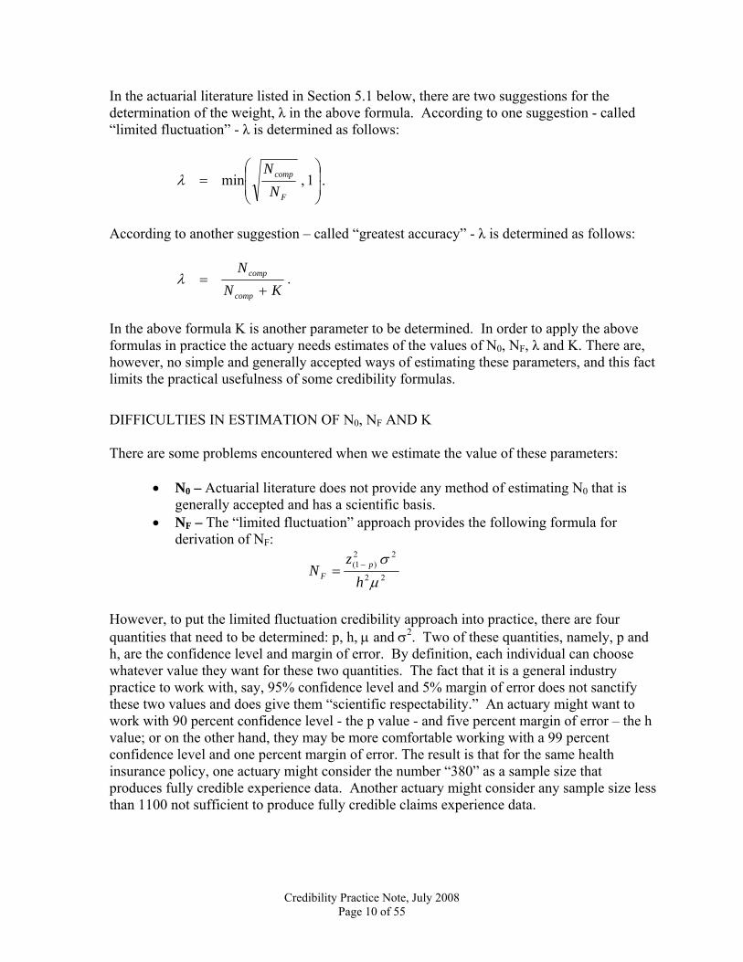
In the actuarial literature listed in Section 5.1 below, there are two suggestions for the determination of the weight, λ in the above formula. According to one suggestion - called “limited fluctuation” - λ is determined as follows:

⎟⎟

⎠

⎞

⎜⎜

⎝

⎛= 1,min

F

comp

NN

λ .

According to another suggestion – called “greatest accuracy” - λ is determined as follows:

KNN

comp

comp

+=λ .

In the above formula K is another parameter to be determined. In order to apply the above formulas in practice the actuary needs estimates of the values of N0, NF, λ and K. There are, however, no simple and generally accepted ways of estimating these parameters, and this fact limits the practical usefulness of some credibility formulas.

DIFFICULTIES IN ESTIMATION OF N0, NF AND K There are some problems encountered when we estimate the value of these parameters:

• N0 – Actuarial literature does not provide any method of estimating N0 that is

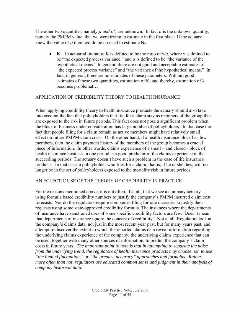
generally accepted and has a scientific basis. • NF – The “limited fluctuation” approach provides the following formula for

derivation of NF:

22

22)1(

μσ

hz

N pF

−=

However, to put the limited fluctuation credibility approach into practice, there are four quantities that need to be determined: p, h, μ and σ2. Two of these quantities, namely, p and h, are the confidence level and margin of error. By definition, each individual can choose whatever value they want for these two quantities. The fact that it is a general industry practice to work with, say, 95% confidence level and 5% margin of error does not sanctify these two values and does give them “scientific respectability.” An actuary might want to work with 90 percent confidence level - the p value - and five percent margin of error – the h value; or on the other hand, they may be more comfortable working with a 99 percent confidence level and one percent margin of error. The result is that for the same health insurance policy, one actuary might consider the number “380” as a sample size that produces fully credible experience data. Another actuary might consider any sample size less than 1100 not sufficient to produce fully credible claims experience data.


The other two quantities, namely μ and σ2, are unknown. In fact μ is the unknown quantity, namely the PMPM value, that we were trying to estimate in the first place. If the actuary knew the value of μ there would be no need to estimate NF.

• K – In actuarial literature K is defined to be the ratio of ν/α, where ν is defined to

be “the expected process variance,” and α is defined to be “the variance of the hypothetical means.” In general there are not good and acceptable estimates of “the expected process variance” and “the variance of the hypothetical means.” In fact, in general, there are no estimates of these parameters. Without good estimates of these two quantities, estimation of K, and thereby, estimation of λ becomes problematic.

APPLICATION OF CREDIBILITY THEORY TO HEALTH INSURANCE

When applying credibility theory to health insurance products the actuary should also take into account the fact that policyholders that file for a claim stay as members of the group that are exposed to the risk in future periods. This fact does not pose a significant problem when the block of business under consideration has large number of policyholders. In that case the fact that people filing for a claim remain as active members might have relatively small effect on future PMPM claim costs. On the other hand, if a health insurance block has few members, then the claim payment history of the members of the group becomes a crucial piece of information. In other words, claims experience of a small – and closed - block of health insurance business in one period is a good predictor of the claims experience in the succeeding periods. The actuary doesn’t have such a problem in the case of life insurance products. In that case, a policyholder who files for a claim, that is, if he or she dies, will no longer be in the set of policyholders exposed to the mortality risk in future periods.

AN ECLECTIC USE OF THE THEORY OF CREDIBILITY IN PRACTICE For the reasons mentioned above, it is not often, if at all, that we see a company actuary using formula based credibility numbers to justify the company’s PMPM incurred claim cost forecasts. Nor do the regulators require companies filing for rate increases to justify their requests using some state-approved credibility formula. The instances where the departments of insurance have sanctioned uses of some specific credibility factors are few. Does it mean that departments of insurance ignore the concept of credibility? Not at all. Regulators look at the company’s claims data, not just in the most recent year past, but for many years past, and attempt to discover the extent to which the reported claims data reveal information regarding the underlying claims experience of the company; the underlying claims experience that can be used, together with many other sources of information, to predict the company’s claim costs in future years. The important point to note is that in attempting to separate the noise from the underlying trend, the regulators of health insurance products may choose not to use “the limited fluctuation,” or “the greatest accuracy” approaches and formulas. Rather, more often than not, regulators use educated common sense and judgment in their analysis of company historical data.


3. Industry Practice

For some time, credibility theory has been applied within the property and casualty industry in order to solve business problems. This has not been the case within the life, annuity and health industries. Therefore, examples of the use of credibility theory and related practices are somewhat difficult to find and somewhat simplistic in their content. With the advent of principle-based approaches for the calculation of reserves and capital, there is a renewed interest among actuaries concerning the use of credibility theory and related approaches in the development of model assumptions. The following examples are a mix of ways that credibility theory or related practices are currently applied within the life, annuity or health industries and some possible solutions that the authors would use to solve the stated problems. Therefore, they are not only intended to illustrate some of the current practices but also some of the practices that have been discussed in various actuarial groups. In order to help the reader become better acquainted with the subject matter, a discussion of the strengths and weaknesses of a particular approach used in the sample is provided after each example. Note that many of these examples presume that an appropriate, identifiable external reference point exists for use with company specific data. This point is also discussed in sections 2.2 and 3.4.


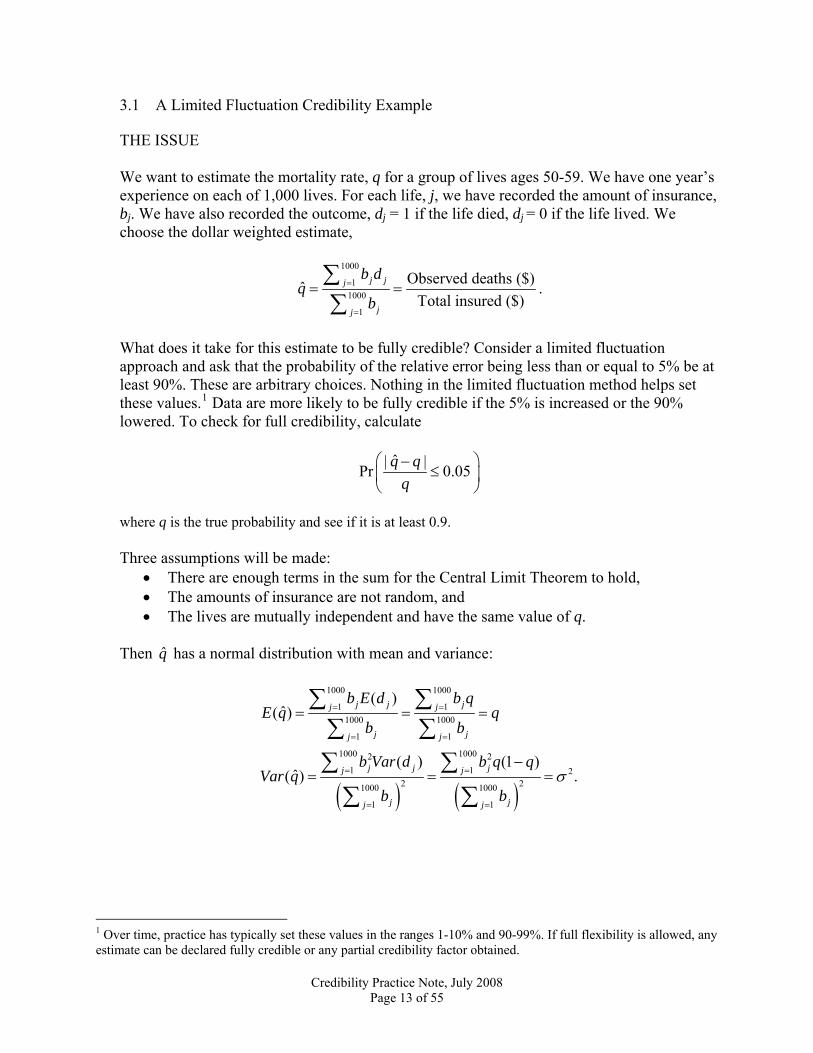
3.1 A Limited Fluctuation Credibility Example THE ISSUE We want to estimate the mortality rate, q for a group of lives ages 50-59. We have one year’s experience on each of 1,000 lives. For each life, j, we have recorded the amount of insurance, bj. We have also recorded the outcome, dj = 1 if the life died, dj = 0 if the life lived. We choose the dollar weighted estimate,

1000

11000

1

Observed deaths ($)ˆTotal insured ($)

j jj

jj

b dq

b=

=

= =∑∑

.

What does it take for this estimate to be fully credible? Consider a limited fluctuation approach and ask that the probability of the relative error being less than or equal to 5% be at least 90%. These are arbitrary choices. Nothing in the limited fluctuation method helps set these values.1 Data are more likely to be fully credible if the 5% is increased or the 90% lowered. To check for full credibility, calculate

ˆ| |Pr 0.05q q

q⎛ ⎞−

≤⎜ ⎟⎝ ⎠

where q is the true probability and see if it is at least 0.9. Three assumptions will be made:

• There are enough terms in the sum for the Central Limit Theorem to hold, 2 • The amounts of insurance are not random, and 3 • The lives are mutually independent and have the same value of q.

Then has a normal distribution with mean and variance: q

( ) ( )

1000 1000

1 11000 1000

1 1

1000 10002 21 1 2

2 21000 1000

1 1

( )ˆ( )

( ) (1 )ˆ( ) .

j j jj j

j jj j

j j jj j

j jj j

b E d b qE q q

b b

b Var d b q qVar q

b bσ

= =

= =

= =

= =

= = =

−= =

∑ ∑∑ ∑

∑ ∑∑ ∑

=

1 Over time, practice has typically set these values in the ranges 1-10% and 90-99%. If full flexibility is allowed, any estimate can be declared fully credible or any partial credibility factor obtained.


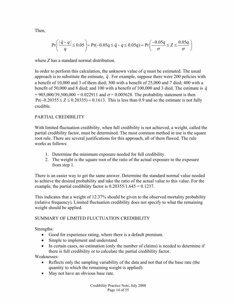
Then,

ˆ| | 0.05 0.05ˆPr 0.05 Pr( 0.05 0.05 ) Prq q q qq q q q Z

q σ σ⎛ ⎞− −⎛ ⎞≤ = − ≤ − ≤ = ≤ ≤⎜ ⎟ ⎜ ⎟

⎝ ⎠⎝ ⎠

where Z has a standard normal distribution. In order to perform this calculation, the unknown value of q must be estimated. The usual approach is to substitute the estimate, . For example, suppose there were 200 policies with a benefit of 10,000 and 3 of them died; 300 with a benefit of 25,000 and 7 died; 400 with a benefit of 50,000 and 8 died; and 100 with a benefit of 100,000 and 3 died. The estimate is = 905,000/39,500,000 = 0.022911 and σ = 0.005628. The probability statement is then

This is less than 0.9 and so the estimate is not fully credible.

q

q

Pr( 0.20355 0.20355) 0.1613.Z− ≤ ≤ =

PARTIAL CREDIBILITY With limited fluctuation credibility, when full credibility is not achieved, a weight, called the partial credibility factor, must be determined. The most common method in use is the square root rule. There are several justifications for this approach, all of them flawed. The rule works as follows:

1. Determine the minimum exposure needed for full credibility. 2. The weight is the square root of the ratio of the actual exposure to the exposure

from step 1.

There is an easier way to get the same answer. Determine the standard normal value needed to achieve the desired probability and take the ratio of the actual value to this value. For the example, the partial credibility factor is 0.20355/1.645 = 0.1237. This indicates that a weight of 12.37% should be given to the observed mortality probability (relative frequency). Limited fluctuation credibility does not specify to what the remaining weight should be applied. SUMMARY OF LIMITED FLUCTUATION CREDIBILITY Strengths:

• Good for experience rating, where there is a default premium. • Simple to implement and understand. • In certain cases, no estimation (only the number of claims) is needed to determine if

there is full credibility or to calculate the partial credibility factor. Weaknesses:

• Reflects only the sampling variability of the data and not that of the base rate (the quantity to which the remaining weight is applied).

• May not have an obvious base rate.


• The choices of the two percents (5% and 90% in the example) are arbitrary. • No sound statistical justification exists for the determination of the partial credibility

factor. In particular, most derivations use variance as a measure of quality. However, credibility estimates are biased, making mean square error a more reasonable choice.2

2 As an absurd example, the estimator “5” has a variance of zero, but is not a particularly good estimator of a mortality rate.


3.2 A Greatest Accuracy Credibility Example Greatest accuracy credibility is the most commonly used alternative to limited fluctuation credibility. It is also referred to as Bayesian credibility, linear Bayesian credibility, and Buhlmann credibility (among other names). All flavors of this method assume that there exists more than one entity (could be an infinite number). Each entity produces numbers according to some probability distribution. For example, the entity could be all the life insurance experience on one company’s block of business and the number is the observed mortality ratio with respect to a standard table. The second assumption is that these probability distributions are themselves distributed among the entities according to another probability distribution. The goal is to then use this information to estimate the probability distribution (or a key parameter of that distribution) for one or all of the entities. THE ISSUE An illustration of this method is in the paper “Empirical Bayesian Credibility for Workers’ Compensation Classification Ratemaking” by Glenn Meyers (Proceedings of the CAS, Vol. LXXI, 1984, pp. 96-121). I have slightly simplified the problem in this description. The entities are 319 occupation classes for workers compensation insurance.3 Each class contributed three numbers, the average claim payments per covered worker in each of three years. In addition, the number of covered workers in each class each year was recorded. The objective is to estimate the true expected payments per worker in each class. One possible model (not a very good one) is to make the following assumptions:

• All members of a given entity (occupation class) have the same distribution. • Observations from a given entity both within one year and from year to year are

mutually independent. • For an individual in a given class, the distribution of claims is normal with a mean

that depends on the class but a variance (v) that is the same for all classes and is known.

• The class means are normally distributed with a known mean (μ) and variance (a). • Mean square error will be minimized to determine the estimate.

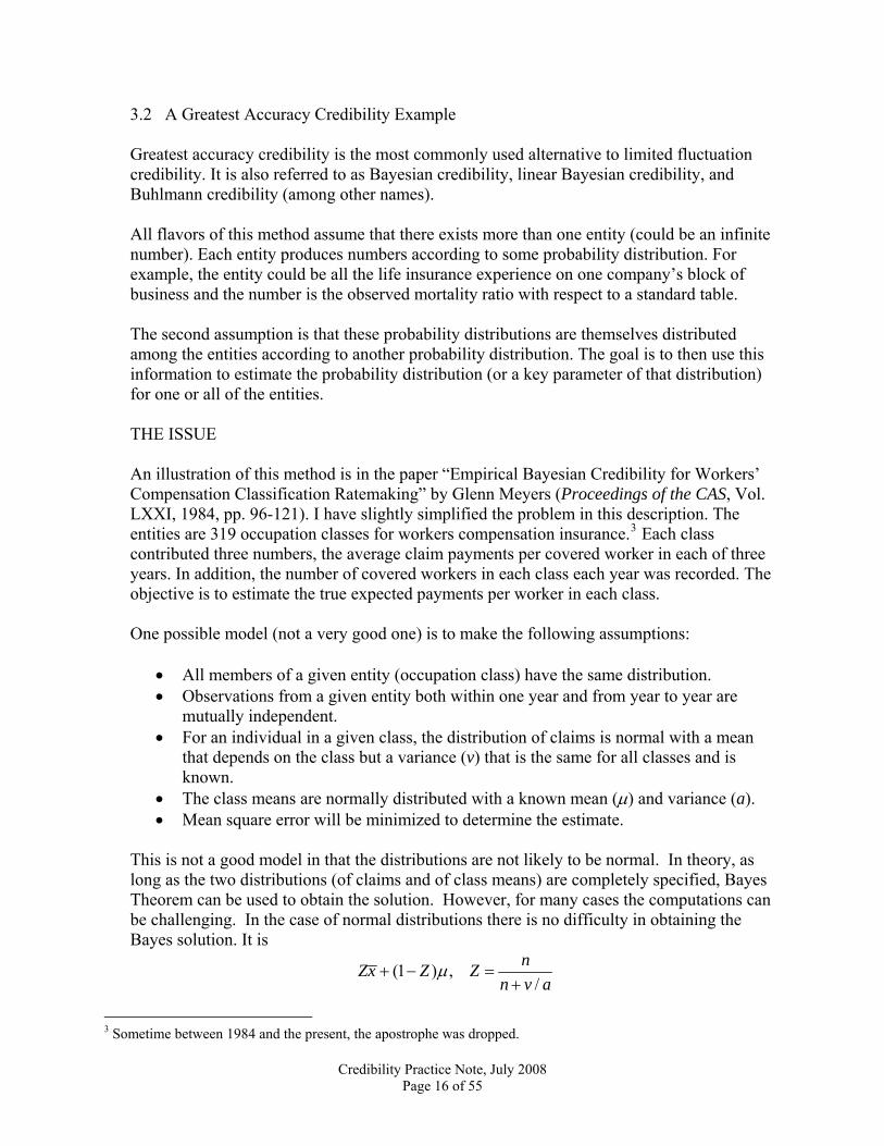
This is not a good model in that the distributions are not likely to be normal. In theory, as long as the two distributions (of claims and of class means) are completely specified, Bayes Theorem can be used to obtain the solution. However, for many cases the computations can be challenging. In the case of normal distributions there is no difficulty in obtaining the Bayes solution. It is

(1 ) ,/

nZx Z Zn v a

μ+ − =+

3 Sometime between 1984 and the present, the apostrophe was dropped.


where n is the total sample size for the three years for the class and x is the sample mean for a given class.

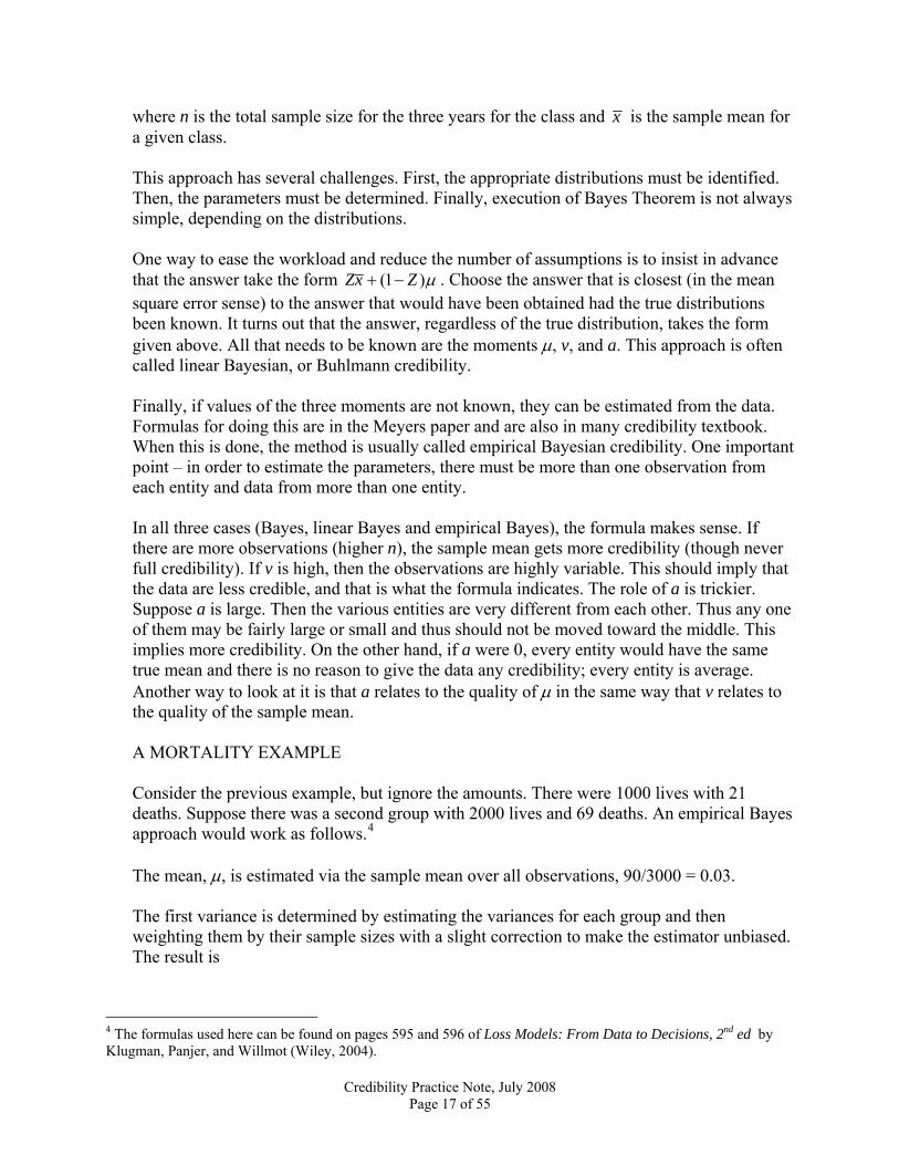
This approach has several challenges. First, the appropriate distributions must be identified. Then, the parameters must be determined. Finally, execution of Bayes Theorem is not always simple, depending on the distributions. One way to ease the workload and reduce the number of assumptions is to insist in advance that the answer take the form (1 )Zx Z μ+ − . Choose the answer that is closest (in the mean square error sense) to the answer that would have been obtained had the true distributions been known. It turns out that the answer, regardless of the true distribution, takes the form given above. All that needs to be known are the moments μ, v, and a. This approach is often called linear Bayesian, or Buhlmann credibility. Finally, if values of the three moments are not known, they can be estimated from the data. Formulas for doing this are in the Meyers paper and are also in many credibility textbook. When this is done, the method is usually called empirical Bayesian credibility. One important point – in order to estimate the parameters, there must be more than one observation from each entity and data from more than one entity. In all three cases (Bayes, linear Bayes and empirical Bayes), the formula makes sense. If there are more observations (higher n), the sample mean gets more credibility (though never full credibility). If v is high, then the observations are highly variable. This should imply that the data are less credible, and that is what the formula indicates. The role of a is trickier. Suppose a is large. Then the various entities are very different from each other. Thus any one of them may be fairly large or small and thus should not be moved toward the middle. This implies more credibility. On the other hand, if a were 0, every entity would have the same true mean and there is no reason to give the data any credibility; every entity is average. Another way to look at it is that a relates to the quality of μ in the same way that v relates to the quality of the sample mean. A MORTALITY EXAMPLE Consider the previous example, but ignore the amounts. There were 1000 lives with 21 deaths. Suppose there was a second group with 2000 lives and 69 deaths. An empirical Bayes approach would work as follows.4 The mean, μ, is estimated via the sample mean over all observations, 90/3000 = 0.03. The first variance is determined by estimating the variances for each group and then weighting them by their sample sizes with a slight correction to make the estimator unbiased. The result is

4 The formulas used here can be found on pages 595 and 596 of Loss Models: From Data to Decisions, 2nd ed by Klugman, Panjer, and Willmot (Wiley, 2004).


1000(0.021)(0.979) 2000(0.0345)(0.9655)ˆ 0.029079

999 1999v +

= =+

The estimate of a is less obvious, due to corrections needed to make it unbiased. It is

2 2

2 21000(0.021 0.03) 2000(0.0345 0.03) 0.029079(2 1)ˆ 0.000069316

1000 200030003000

a − + − − −= =

+−

For the first group,

1000 0.704470.02907910000.000069316

Z = =+

and the credibility estimate is 0.70447(0.21) + 0.29553(0.03) = 0.023660. SUMMARY OF GREATEST ACCURACY CREDIBILITY Strengths:

• All aspects of the process are clearly spelled out. Any approximations or assumptions made are clearly stated.

• Once the assumptions and objectives are in place, an exact answer can be obtained from basic probability principles.

• There is a clear objective function – minimizing mean square error. • There are no arbitrary choices that are unrelated to the observed random variables.

Weaknesses:

• The linear Bayes approximation may be poor, particularly if the random variable has a heavy tail.

• The usual empirical Bayes estimate of a can be negative (because a is a variance, the true value cannot be negative).

• Unless the prior distribution is known from some other knowledge source, it can only be estimated if there is data from more than one entity.


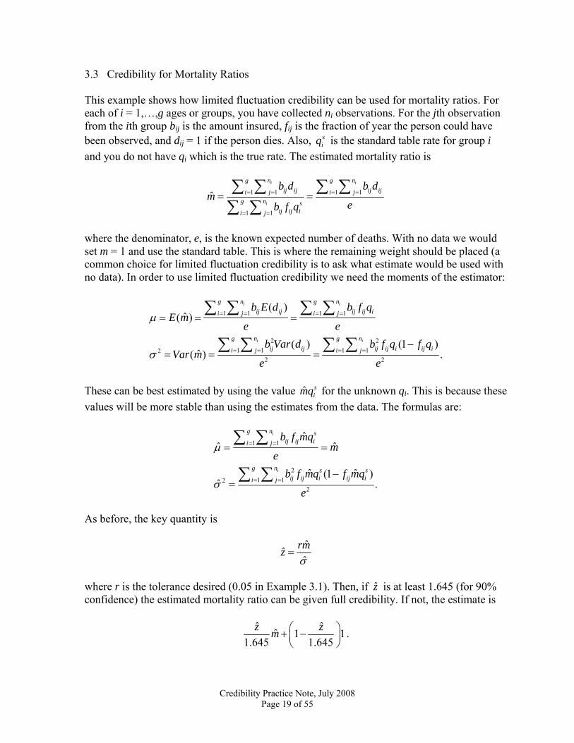
3.3 Credibility for Mortality Ratios This example shows how limited fluctuation credibility can be used for mortality ratios. For each of i = 1,…,g ages or groups, you have collected ni observations. For the jth observation from the ith group bij is the amount insured, fij is the fraction of year the person could have been observed, and dij = 1 if the person dies. Also, s

iq is the standard table rate for group i and you do not have qi which is the true rate. The estimated mortality ratio is

1 1 1 1

1 1

ˆi i

i

g n g nij ij ij iji j i j

g n sij ij ii j

b d b dm

eb f q= = = =

= =

= =∑ ∑ ∑ ∑

∑ ∑

where the denominator, e, is the known expected number of deaths. With no data we would set m = 1 and use the standard table. This is where the remaining weight should be placed (a common choice for limited fluctuation credibility is to ask what estimate would be used with no data). In order to use limited fluctuation credibility we need the moments of the estimator:

1 1 1 1

2 21 1 1 12

2 2

( )ˆ( )

( ) (1 )ˆ( ) .

i i

i i

g n g nij ij ij ij ii j i j

g n g nij ij ij ij i ij ii j i j

b E d b f qE m

e eb Var d b f q f q

Var me e

μ

σ

= = = =

= = = =

= = =

−= = =

∑ ∑ ∑ ∑

∑ ∑ ∑ ∑

These can be best estimated by using the value ˆ s

imq for the unknown qi. This is because these values will be more stable than using the estimates from the data. The formulas are:

1 1

21 12

2

ˆˆ ˆ

ˆ ˆ(1 )ˆ .

i

i

g n sij ij ii j

g n s sij ij i ij ii j

b f mqm

eb f mq f mq

e

μ

σ

= =

= =

= =

−=

∑ ∑

∑ ∑

As before, the key quantity is

ˆˆˆ

rmzσ

=

where r is the tolerance desired (0.05 in Example 3.1). Then, if is at least 1.645 (for 90% confidence) the estimated mortality ratio can be given full credibility. If not, the estimate is

z

ˆ ˆˆ 1 11.645 1.645

z zm ⎛ ⎞+ −⎜ ⎟⎝ ⎠

.


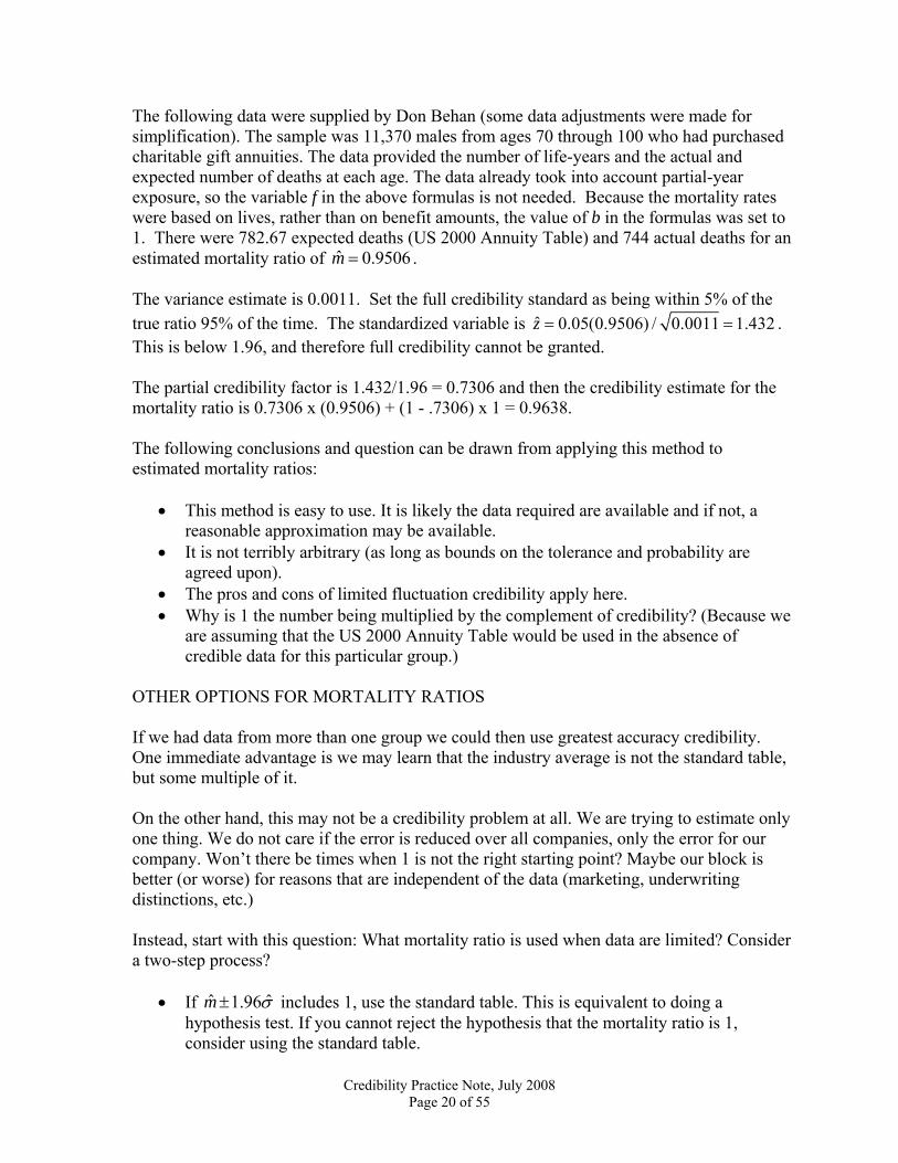
The following data were supplied by Don Behan (some data adjustments were made for simplification). The sample was 11,370 males from ages 70 through 100 who had purchased charitable gift annuities. The data provided the number of life-years and the actual and expected number of deaths at each age. The data already took into account partial-year exposure, so the variable f in the above formulas is not needed. Because the mortality rates were based on lives, rather than on benefit amounts, the value of b in the formulas was set to 1. There were 782.67 expected deaths (US 2000 Annuity Table) and 744 actual deaths for an estimated mortality ratio of . ˆ 0.9506m = The variance estimate is 0.0011. Set the full credibility standard as being within 5% of the true ratio 95% of the time. The standardized variable is ˆ 0.05(0.9506) / 0.0011 1.432z = = . This is below 1.96, and therefore full credibility cannot be granted. The partial credibility factor is 1.432/1.96 = 0.7306 and then the credibility estimate for the mortality ratio is 0.7306 x (0.9506) + (1 - .7306) x 1 = 0.9638. The following conclusions and question can be drawn from applying this method to estimated mortality ratios:

• This method is easy to use. It is likely the data required are available and if not, a reasonable approximation may be available.

• It is not terribly arbitrary (as long as bounds on the tolerance and probability are agreed upon).

• The pros and cons of limited fluctuation credibility apply here. • Why is 1 the number being multiplied by the complement of credibility? (Because we

are assuming that the US 2000 Annuity Table would be used in the absence of credible data for this particular group.)

OTHER OPTIONS FOR MORTALITY RATIOS If we had data from more than one group we could then use greatest accuracy credibility. One immediate advantage is we may learn that the industry average is not the standard table, but some multiple of it. On the other hand, this may not be a credibility problem at all. We are trying to estimate only one thing. We do not care if the error is reduced over all companies, only the error for our company. Won’t there be times when 1 is not the right starting point? Maybe our block is better (or worse) for reasons that are independent of the data (marketing, underwriting distinctions, etc.) Instead, start with this question: What mortality ratio is used when data are limited? Consider a two-step process? 1

• If ˆ1.96m σ± includes 1, use the standard table. This is equivalent to doing a hypothesis test. If you cannot reject the hypothesis that the mortality ratio is 1, consider using the standard table.


• If the interval does not contain 1, use one of the endpoints of the interval. The appropriate endpoint depends on the ultimate use of the ratio. The interval will not contain 1 either if the estimated ratio is far from 1 or if the sample size is large (reducing the standard deviation). Either case is an argument for not using the standard table. However, in all cases, estimation error will still be accounted for (so there is never full credibility).

In the example, 1 is in the confidence interval, so this method would indicate that the data do not justify deviating from the standard table.


3.4 Practical Considerations for Credibility in Reinsurance Pricing

In pricing individual life reinsurance for a client (a direct insurer), an application of credibility theory is needed to blend a starting-point mortality table with the client’s own mortality experience. In many cases the starting-point mortality table is the reinsurer’s client-specific mortality table death rates derived from seriatim internal and client-provided data, with adjustments to take into account underwriting requirements and preferred criteria, but set to an overall level of mortality that may differ from experience for the client whose account is being priced. One of the most important questions is typically, “how closely should the pricing mortality resemble the client’s experience?” The first step in determining an answer to this question is to apply credibility theory, but there are several important matters to consider before finalizing the mortality assumption. One major consideration is how relevant the client’s mortality experience is to the product being priced. If the product specifications, underwriting requirements, preferred criteria, underwriting staff, and distribution channels are all identical between the product being priced and the available mortality experience, then this should not be an issue. But if a new chief underwriter has since taken over, requirements have been strengthened, and a preferred class has been added, then perhaps a little less emphasis should be placed on the experience, and the effect of these changes should be incorporated into the pricing mortality by means other than the application of credibility.

Another consideration is the base mortality table that is used. If the experience is being blended with a mortality table that is very credible but is generic to the insurance industry and is based on experience from an era when not much preferred business was being issued, then the pricing mortality could be allowed to be more heavily influenced by a small to medium amount of credibility in the client’s experience. But if the experience is being blended with a credible mortality table that was derived from recent insured lives experience from other companies but adjusted to account for the client’s own underwriting, claims, and marketing practices, then it might take more experience data from the client to have as much of an effect on the pricing mortality. Yet another consideration is to what extent the mortality slopes (relative mortality by age, gender, duration, risk class, etc.) in the client’s experience should be reflected in the pricing mortality. In most situations, the credibility of the overall experience is questionable enough that partitioning the experience data to compare mortality among subgroups results in such low credibility that it is not worth the effort of going through the exercise of blending the experience with the base mortality table at the cell level. But situations do arise when there is a different mortality pattern that is specific to a certain company and there is enough credibility in the subgroups that it should be incorporated into the pricing mortality. When this happens, credibility theory can be applied to determine to what extent that pattern is reflected in the mortality assumption and the overall level of mortality can be further adjusted based on the credibility of the experience in total.


Once all of these considerations have been addressed, the pricing actuary can determine adjustments to make to the credibility weight that is to be applied to the client’s mortality experience before blending it with a mortality table. To illustrate an application of credibility in reinsurance pricing using an example, consider a situation where an actuary is pricing a new universal life product for ABC Life. ABC Life has only issued term policies in the past, so they supplied experience data for those plans, since it will be sold through the same distribution channels and the underwriting staff is the same. However, with the introduction of the new UL product, they are adding a super preferred non-tobacco class.

ABC Life’s mortality experience study results in an overall actual-to-expected (A/E) ratio of 110% relative to the reinsurer’s base mortality table. The pricing actuary notices unusually high mortality in the preferred tobacco class, but since there are only 20 claims in that class the actuary decides to use the relationships already established in the base table rather than go through the effort to reshape the mortality slope by preferred class for this client with this limited amount of additional experience. Instead, the actuary will focus efforts on using the client’s experience to make an adjustment to the overall level of mortality in the base table. More discussion on addressing client-specific mortality slopes appears later in this example. Note that the A/E ratio in the experience study is relative to a version of the base table that only has two non-tobacco classes, while the base table used for pricing the new product was derived on an equivalent basis, but includes the additional super preferred class. For illustrative purposes in this example, let’s say the actuary, using formulas and parameters consistent with prior reinsurance pricing exercises, arrives at a credibility weight of 70%. Since the study did not include a super preferred class, the actuary may choose to reduce the credibility factor by several percent, perhaps to 63%. The study being based on term and not UL might suggest that the percentage be further reduced to 60%. It should be noted that in this example these reductions to the credibility weight are based strictly on actuarial judgment.

A credibility weight of 60% and an A/E ratio of 110% results in the actuary setting the final pricing mortality assumption at 106% ( = 60% x 110% + 40% x 100%) of the base table. Getting back to client-specific mortality slopes, it should be noted that if there is an underlying reason for a client’s experience to show mortality by class within any given category that has a different shape than what the base table assumes, then it should probably be reflected in the mortality assumption used in pricing that client’s reinsurance. In the above example, if there is no reason to believe the elevated mortality in the preferred tobacco class is caused by something systematically different in that client’s underwriting relative to all other clients, then it could be assumed that it was just a random fluctuation since there were only 20 claims. It should not be reflected in the mortality assumption by adjusting preferred tobacco mortality up and the other classes down.


An example where an actuary should consider a client-specific slope adjustment might be where a client includes comments in their underwriters’ training manual to direct them to allow fewer exceptions when applying preferred criteria for ages 50 and above, and as a result their mortality experience shows lower A/E ratios at these ages. If no adjustment is made to the age slope in the mortality table, the reinsurer is left open to distribution risk, meaning that if the age distribution of policies issued in the future shifts toward the younger ages, the overall A/E ratios of future experience studies will go up. Also, if the client insurance company does not reflect in the premiums the differences by age in how the company applies the preferred criteria, it will likely cause premiums for ages 50 and above to be less attractive to potential applicants, speeding up the undesirable shift in the age distribution.


3.5 Practical Considerations for using Credibility for Mortality This example describes practical considerations in applying credibility theory to develop or support mortality assumptions. The example presents a practical framework in approaching the setting of mortality assumptions. The example uses an approach that is an admittedly less theoretically grounded approach than others in practice. MORTALITY ASSUMPTION When actuaries build their models, they use assumptions they believe appropriate. For mortality, this is usually k% or .01K of a known mortality table. PRE STUDY DATA HANDLING Inforce files and transaction data are checked and reconciled and any data deficiency is corrected or noted before an experience study is completed. MORTALITY STUDY There are factors to consider when performing a mortality study. It could be a valuation study which uses grouped inforce data at valuation dates and the decrement transactions in between valuation dates. It could be a seriatim study which tracks the status of each policy thru a study period. Some mortality studies aim to create a new mortality table, using the actual number or amount of deaths/exposure as an estimate of the death rate. Another fairly common approach is to compute an expected number or amount of deaths based on a specific table by multiplying the exposure amount by the known tabular death rate. This expected amount may also be known as the tabular amount or number of deaths, since it is the tabular death rate that was applied to the exposure. The actual deaths-to-tabular deaths (A/T) ratio is the experienced tracked. Another name for this A/T Ratio is the Mortality Ratio (MR). For this example, this is the mortality study approach adopted. Some considerations in the grouping of the results are product or death benefit type, age brackets, durations or issue year groupings. These considerations are to be consistent with the way the assumptions will be used in the actuarial models. USE OF CREDIBILITY Credibility may be used when the mortality experience is to be weighted against either a prescribed mortality table or a known industry standard table. A simple approach is to weigh the experienced MR by credibility factors based on the number of deaths. The company may either decide to develop its own credibility weights or use factors developed in existing literature.


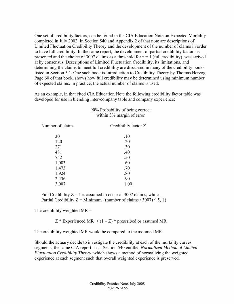
One set of credibility factors, can be found in the CIA Education Note on Expected Mortality completed in July 2002. In Section 540 and Appendix 2 of that note are descriptions of Limited Fluctuation Credibility Theory and the development of the number of claims in order to have full credibility. In the same report, the development of partial credibility factors is presented and the choice of 3007 claims as a threshold for z = 1 (full credibility), was arrived at by consensus. Descriptions of Limited Fluctuation Credibility, its limitations, and determining the claims to meet full credibility are discussed in many of the credibility books listed in Section 5.1. One such book is Introduction to Credibility Theory by Thomas Herzog. Page 60 of that book, shows how full credibility may be determined using minimum number of expected claims. In practice, the actual number of claims is used. As an example, in that cited CIA Education Note the following credibility factor table was developed for use in blending inter-company table and company experience:

90% Probability of being correct

within 3% margin of error Number of claims Credibility factor Z

30 .10 120 .20 271 .30 481 .40 752 .50 1,083 .60 1,473 .70 1,924 .80 2,436 .90 3,007 1.00

Full Credibility Z = 1 is assumed to occur at 3007 claims, while Partial Credibility Z = Minimum {(number of claims / 3007) ^.5, 1} The credibility weighted MR = Z * Experienced MR + (1 – Z) * prescribed or assumed MR The credibility weighted MR would be compared to the assumed MR. Should the actuary decide to investigate the credibility at each of the mortality curves segments, the same CIA report has a Section 540 entitled Normalized Method of Limited Fluctuation Credibility Theory, which shows a method of normalizing the weighted experience at each segment such that overall weighted experience is preserved.


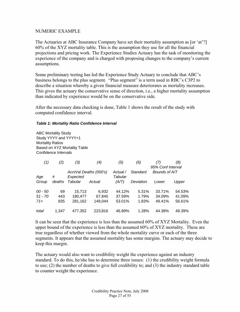
NUMERIC EXAMPLE The Actuaries at ABC Insurance Company have set their mortality assumption as [or ‘at’?] 60% of the XYZ mortality table. This is the assumption they use for all the financial projections and pricing work. The Experience Studies Actuary has the task of monitoring the experience of the company and is charged with proposing changes to the company’s current assumptions. Some preliminary testing has led the Experience Study Actuary to conclude that ABC’s business belongs to the plus segment. “Plus segment” is a term used in RBC’s C3P2 to describe a situation whereby a given financial measure deteriorates as mortality increases. This gives the actuary the conservative sense of direction, i.e., a higher mortality assumption than indicated by experience would be on the conservative side. After the necessary data checking is done, Table 1 shows the result of the study with computed confidence interval. Table 1: Mortality Ratio Confidence Interval

ABC Mortality StudyStudy YYYY and YYYY+1Mortality RatiosBased on XYZ Mortality TableConfidence Intervals

(1) (2) (3) (4) (5) (6) (7) (8)95% Conf Interval

AcctVal Deaths (000's) Actual / Standard Bounds of A/TAge Group

# deaths

Expected Tabular Actual

Tabular (A/T) Deviation Lower Upper

00 - 50 69 15,713 6,932 44.12% 5.31% 33.71% 54.53%51 - 70 443 180,477 67,840 37.59% 1.79% 34.09% 41.09%71+ 835 281,162 149,044 53.01% 1.83% 49.41% 56.61%

total 1,347 477,352 223,816 46.89% 1.28% 44.38% 49.39% It can be seen that the experience is less than the assumed 60% of XYZ Mortality. Even the upper bound of the experience is less than the assumed 60% of XYZ mortality. These are true regardless of whether viewed from the whole mortality curve or each of the three segments. It appears that the assumed mortality has some margins. The actuary may decide to keep this margin. The actuary would also want to credibility weight the experience against an industry standard. To do this, he/she has to determine three issues: (1) the credibility weight formula to use; (2) the number of deaths to give full credibility to; and (3) the industry standard table to counter weight the experience.


The Experience Study Actuary has decided to use the following credibility weight formula: Z = minimum { (number of deaths / number of deaths with full credibility)^.5, 1) with the full credibility assumed to occur at 3007 deaths. The actuary has based this on Section 540 and Appendix 2 of the July 2002 CIA Education Note. In Section 540, the consensus minimum number of deaths recommended for 100% credibility was 3007. A more theoretical approach would have been to actually compute the credibility weights as described elsewhere in the practice note. The Experience Study Actuary chose the 1994 MGDB mortality table as the standard table to “counterbalance” against the experience. This was chosen on three grounds: (1) it is a recognizable standard table; (2) it was based on an industry wide study; and (3) it is the prescribed mortality table for similar products. Since the company uses the XYZ table which is different from the standard table (e.g., 1994 MGDB), it would be necessary to translate the standard table to a percentage of the XYZ table that the company is using. It was determined beforehand that the XYZ mortality for this business is 133% of the standard valuation table (e.g., the 1994 MGDB mortality table is 75% of XYZ mortality). For each of the age segments, the expected based on the standard valuation table to the expected based on the tabular XYZ mortality table were noted and will be used as the “industry” actual-to-expected ratio counterbalancing the experience. To illustrate this, in Table 2 the ratio of the Standard table to table that the company uses is 42.96% for ages 0-50, 70% for ages 51-70, 80% ages 71 above, for an overall ratio of the Standard table of 70% of the Table the company uses. Table 2 shows the credibility weighting of the mortality experience (overall 66.93% of XYZ table) versus that expected by the standard industry table (overall 75% of XYZ table). Table 2: Credibility Weighted Mortality Ratio

ABC Mortality StudyStudy YYYY and YYYY+1Mortality RatiosBased on XYZ Mortality TableCredibility Weighted

(1) (2) (3) (4) (5) (6) (7) (8) (9) (10) (11)AcctVal Deaths (000's) Actual/ weight Z Standard Standard Cred.Wtd Expected Deaths

Age Group

# deaths

Expected Tabular Actual

Tabular (A/T)

Table Expected

Table to Tabular Mort Ratios Credibility Weighted

00 - 50 69 15,713 6,932 44.12% 15.15% 6,751 42.96% 43.14% 6,778 39.14%51 - 70 443 180,477 67,840 37.59% 38.38% 126,334 70.00% 57.56% 103,882 52.22%71+ 835 281,162 149,044 53.01% 52.70% 224,930 80.00% 65.78% 184,941 59.68%

total 1,347 477,352 223,816 46.89% 66.93% 358,014 75.00% 56.18% 268,196 56.18%295,601

Normalizationfactor: 0.90729

Column (5) is the Actual to Tabular Mortality Ratio Raw experience.


Column (6) is the credibility weights to be used based on Full Credibility. Column (8) is the industry Mortality Ratio to be counter weighted against. Column (9) is the credibility weighted Mortality Ratio experience. The overall credibility mortality ratio is 56.18% which is less than the assumed 60%. The actuary may normalize the MR at each age segment so that the sum of expected deaths for all the segments preserves the total produced by the blended overall MR. This may be seen in Column (11). The actuary may observe the blended mortality ratio at the overall level (56.18%) and at the segment level after normalization (39.14%, 52.22%, 59.68%) and draw a conclusion as to acceptability of keeping the current mortality ratio assumption or redo the MR assumption. Knowing that this block of business belongs to the plus segment gives the actuary a sense of direction as far as whether margins exist. In this case, experience is favorable from both the confidence interval view (upper bound of the experience is less than assumed MR) and the overall credibility weighted MR (lower then the assumed MR). This would lead the actuary to propose no change in mortality assumption for this block. The experience for the block is monitored each year and any historical trends are considered in the decision to keep or revise the assumed mortality for the block.


3.6 An Example Using Limited Fluctuation Credibility to Update Lapse Assumptions An Insurance company is undergoing the process of updating the lapse assumptions in their projection models. The same process has been used for several years. At a high level, the process requires three basic steps: the first is to obtain experience data from the Insurance In-force Management group; the next step is to enter the data into an existing worksheet; the final step is to review the results and update the projection model. The experience data is for a Variable Universal Life (VUL) product with seven study-years (1999-2005) Actual Lapse Rates= (LAPSE+REPLACED+SURRENDER)/(LAPSE+REPLACED+SURRENDER+INFORCE)

1 2 3 4 5 6 7 8 9 10 11 12 13 14 15 16+0 to 34 7.0% 10.6% 9.5% 8.7% 7.5% 8.4% 7.7% 7.3% 7.7% 7.3% 8.4% 7.6% 6.8% 6.6% 6.7% 7.2%35 to 44 6.2% 9.1% 9.0% 7.5% 6.9% 7.0% 6.8% 6.3% 6.1% 6.5% 7.9% 7.0% 7.2% 7.1% 7.6% 7.5%45 to 54 5.1% 7.4% 7.2% 6.6% 5.8% 6.3% 6.3% 6.1% 6.5% 7.2% 8.6% 8.7% 7.7% 8.9% 8.4% 7.7%55 to 59 4.1% 6.2% 5.0% 5.8% 5.5% 6.1% 6.5% 6.2% 6.4% 8.8% 10.8% 11.4% 8.5% 11.7% 11.1% 10.8%60 to 64 2.7% 5.4% 4.2% 6.1% 5.5% 6.2% 6.5% 7.1% 6.5% 8.7% 10.6% 10.2% 10.7% 12.4% 9.4% 12.4%65 to 69 3.8% 4.8% 6.2% 6.5% 6.6% 7.3% 8.5% 6.1% 8.6% 8.2% 8.1% 8.9% 6.6% 11.2% 2.9% 12.3%70 to 74 2.3% 4.5% 6.1% 6.8% 8.1% 7.8% 9.8% 6.7% 10.8% 8.7% 10.8% 9.5% 8.9% 17.8% 7.4% 3.3%75 to 99 1.9% 9.5% 6.4% 8.9% 6.1% 9.7% 10.3% 10.0% 8.0% 7.1% 10.7% 2.1% 10.5% 4.9% 1.8% 10.1% Exposure Count Policies = n

1 2 3 4 5 6 7 8 9 10 11 12 13 14 15 16+0 to 34 25,090 30,887 35,307 39,154 37,684 36,282 33,285 30,283 26,337 22,554 18,568 16,279 12,927 9,387 6,556 10,65935 to 44 18,695 24,447 29,859 35,118 35,928 36,187 33,975 30,878 27,047 22,716 17,785 14,959 11,338 7,926 5,482 8,52345 to 54 14,124 18,099 21,801 25,641 25,352 24,571 21,832 18,834 15,688 12,329 8,626 6,866 4,756 3,134 2,099 3,17055 to 59 3,627 4,665 5,748 6,810 6,612 6,355 5,587 4,717 3,873 2,930 1,983 1,619 1,114 747 511 76760 to 64 1,809 2,446 3,137 3,802 3,772 3,650 3,260 2,785 2,274 1,715 1,129 899 617 409 277 40565 to 69 988 1,373 1,777 2,153 2,177 2,137 1,924 1,591 1,306 978 663 523 333 223 152 22270 to 74 562 868 1,155 1,418 1,409 1,368 1,227 1,016 808 582 372 281 195 130 88 10775 to 99 436 618 772 945 902 847 713 564 425 300 180 127 84 52 39 52

The process consists of 4 steps: 1) The table below is in the worksheet. This is the “base” table for credibility application. Assumed Base plan lapse rate = p

1 2 3 4 5 6 7 8 9 10 11 12 13 14 15 16+0 to 34 3.0% 3.0% 5.0% 7.0% 7.0% 7.0% 7.0% 7.0% 7.0% 7.0% 7.0% 7.0% 7.0% 7.0% 7.5% 8.0%35 to 44 2.0% 2.0% 3.5% 4.0% 4.5% 4.5% 4.5% 5.0% 5.5% 5.5% 6.5% 6.0% 6.5% 7.0% 7.5% 8.0%45 to 54 2.0% 2.0% 3.0% 3.5% 4.0% 4.0% 4.5% 5.0% 5.5% 5.5% 6.5% 6.0% 6.5% 7.0% 7.5% 8.0%55 to 59 2.0% 2.0% 3.0% 3.5% 4.0% 4.0% 4.5% 5.0% 5.5% 5.5% 6.5% 6.0% 6.5% 7.0% 7.5% 8.0%60 to 64 2.0% 2.0% 3.0% 3.5% 4.0% 4.0% 4.5% 5.0% 5.5% 5.5% 6.5% 6.0% 6.5% 7.0% 7.5% 8.0%65 to 69 2.0% 2.0% 3.0% 3.5% 4.0% 4.0% 4.5% 5.0% 5.5% 5.5% 6.5% 6.0% 6.5% 7.0% 7.5% 8.0%70 to 74 2.0% 2.0% 3.0% 3.5% 4.0% 4.0% 4.5% 5.0% 5.5% 5.5% 6.5% 6.0% 6.5% 7.0% 7.5% 8.0%75 to 99 2.0% 2.0% 3.0% 3.5% 4.0% 4.0% 4.5% 5.0% 5.5% 5.5% 6.5% 6.0% 6.5% 7.0% 7.5% 8.0% 2) Next, the Expected Lapse Count is calculated by multiplying the Assumed Base Plan Lapse rate by the Exposure Count. Expected Lapse Count = n * p

1 2 3 4 5 6 7 8 9 10 11 12 13 14 15 16+0 to 34 753 927 1,765 2,741 2,638 2,540 2,330 2,120 1,844 1,579 1,300 1,140 905 657 492 85335 to 44 374 489 1,045 1,405 1,617 1,628 1,529 1,544 1,488 1,249 1,156 898 737 555 411 68245 to 54 282 362 654 897 1,014 983 982 942 863 678 561 412 309 219 157 25455 to 59 73 93 172 238 264 254 251 236 213 161 129 97 72 52 38 6160 to 64 36 49 94 133 151 146 147 139 125 94 73 54 40 29 21 3265 to 69 20 27 53 75 87 85 87 80 72 54 43 31 22 16 11 1870 to 74 11 17 35 50 56 55 55 51 44 32 24 17 13 9 7 975 to 99 9 12 23 33 36 34 32 28 23 17 12 8 5 4 3 4


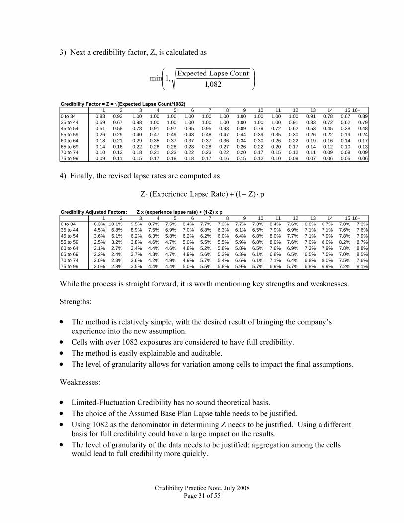
3) Next a credibility factor, Z, is calculated as

⎟⎟⎠

⎞⎜⎜⎝

⎛

082,1CountLapseExpected,1min

1 2 3 4 5 6 7 8 9 10 11 12 13 14 15 16+

0 to 34 0.83 0.93 1.00 1.00 1.00 1.00 1.00 1.00 1.00 1.00 1.00 1.00 0.91 0.78 0.67 0.8935 to 44 0.59 0.67 0.98 1.00 1.00 1.00 1.00 1.00 1.00 1.00 1.00 0.91 0.83 0.72 0.62 0.7945 to 54 0.51 0.58 0.78 0.91 0.97 0.95 0.95 0.93 0.89 0.79 0.72 0.62 0.53 0.45 0.38 0.4855 to 59 0.26 0.29 0.40 0.47 0.49 0.48 0.48 0.47 0.44 0.39 0.35 0.30 0.26 0.22 0.19 0.2460 to 64 0.18 0.21 0.29 0.35 0.37 0.37 0.37 0.36 0.34 0.30 0.26 0.22 0.19 0.16 0.14 0.1765 to 69 0.14 0.16 0.22 0.26 0.28 0.28 0.28 0.27 0.26 0.22 0.20 0.17 0.14 0.12 0.10 0.1370 to 74 0.10 0.13 0.18 0.21 0.23 0.22 0.23 0.22 0.20 0.17 0.15 0.12 0.11 0.09 0.08 0.0975 to 99 0.09 0.11 0.15 0.17 0.18 0.18 0.17 0.16 0.15 0.12 0.10 0.08 0.07 0.06 0.05 0.06

Credibility Factor = Z = √(Expected Lapse Count/1082)

4) Finally, the revised lapse rates are computed as

p)Z1()RateLapseExperience(Z ⋅−+⋅

1 2 3 4 5 6 7 8 9 10 11 12 13 14 15 16+

0 to 34 6.3% 10.1% 9.5% 8.7% 7.5% 8.4% 7.7% 7.3% 7.7% 7.3% 8.4% 7.6% 6.8% 6.7% 7.0% 7.3%35 to 44 4.5% 6.8% 8.9% 7.5% 6.9% 7.0% 6.8% 6.3% 6.1% 6.5% 7.9% 6.9% 7.1% 7.1% 7.6% 7.6%45 to 54 3.6% 5.1% 6.2% 6.3% 5.8% 6.2% 6.2% 6.0% 6.4% 6.8% 8.0% 7.7% 7.1% 7.9% 7.8% 7.9%55 to 59 2.5% 3.2% 3.8% 4.6% 4.7% 5.0% 5.5% 5.5% 5.9% 6.8% 8.0% 7.6% 7.0% 8.0% 8.2% 8.7%60 to 64 2.1% 2.7% 3.4% 4.4% 4.6% 4.8% 5.2% 5.8% 5.8% 6.5% 7.6% 6.9% 7.3% 7.9% 7.8% 8.8%65 to 69 2.2% 2.4% 3.7% 4.3% 4.7% 4.9% 5.6% 5.3% 6.3% 6.1% 6.8% 6.5% 6.5% 7.5% 7.0% 8.5%70 to 74 2.0% 2.3% 3.6% 4.2% 4.9% 4.9% 5.7% 5.4% 6.6% 6.1% 7.1% 6.4% 6.8% 8.0% 7.5% 7.6%75 to 99 2.0% 2.8% 3.5% 4.4% 4.4% 5.0% 5.5% 5.8% 5.9% 5.7% 6.9% 5.7% 6.8% 6.9% 7.2% 8.1%

Credibility Adjusted Factors: Z x (experience lapse rate) + (1-Z) x p

While the process is straight forward, it is worth mentioning key strengths and weaknesses. Strengths: • The method is relatively simple, with the desired result of bringing the company’s

experience into the new assumption. • Cells with over 1082 exposures are considered to have full credibility. • The method is easily explainable and auditable. • The level of granularity allows for variation among cells to impact the final assumptions. Weaknesses: • Limited-Fluctuation Credibility has no sound theoretical basis. • The choice of the Assumed Base Plan Lapse table needs to be justified. • Using 1082 as the denominator in determining Z needs to be justified. Using a different

basis for full credibility could have a large impact on the results. • The level of granularity of the data needs to be justified; aggregation among the cells

would lead to full credibility more quickly.


• The actuary needs to understand the experience data and determine whether it is appropriate to use for the future.

• With the above choices, different actuaries may get different results using the same data. • The results may not be “smooth.” ADDITIONAL CONSIDERATION There are alternative approaches that an actuary could use to build assumptions from experience data. Two examples are an application of regression or Bayesian credibility.


3.7 Credibility Conflict I

PROBLEM A credit insurer has never had any insurance claims but refuses to lower its premium rates. The state’s chief actuary thinks that this is causing insureds to be overcharged. Thus far the insurer has insured one million policies without a claim. How many claims should be expected on its next one million policies? Note: This example is an extreme case and is used to make a point rather than to illustrate a situation likely to be encountered in practice. SOLUTION General Approach - We adopt a Bayesian approach. Assumptions - We make the following assumptions: First, we assume that claims are mutually independent and identically distributed with a binomial distribution with parameter,Θ . So, we use the binomial with parameter, Θ , as our likelihood. Second, we assume that the parameter,Θ , has a prior beta distribution, B(a,b), with parameters and , so that the (prior) mean of the beta distribution is 1a = 999b =

001.99911

baa

=+

=+

.

This estimated mean was obtained from the experience of a large number of policies of some related insurance. This conforms to the approach advocated by Buhlmann as discussed in Section 4 of this work. The implicit sample size selected here is

000,19991ba =+=+ . Some practitioners might feel that we should have used a larger implicit sample size; perhaps, we should have chosen 100a = and 900,99b = . Note: Here we are treating Θ as a random variable. Computations Following the discussion of (1) Theorem 8.1 on pages 135-136 and (2) Exercise 8-2(a) of Herzog [1999], we find that the posterior distribution of Θ is B(a+r,b+n-r) where 0r = is


the number of observed “successes” – i.e., claims – and 000,000,1n = is the number of trials – i.e., exposures, measured by policies. The mean of this posterior distribution is

000,001,11

000,000,1999101

nbara

=+++

=++

+ .

This is a substantial decline from the prior mean that we began with. So, the expected number of claims on the next 1,000,000 policies is

( ) 1000,001,1

1000,000,1 ≅⋅ .

Strengths: • This approach conforms to the underlying mathematical theory. • All of the assumptions made are set forth explicitly.

• The result obtained is a reasonable one. This is in sharp contrast to the results of a

limited fluctuation approach to this problem. Under that paradigm, you end up with a credibility factor of either 1Z = or .0Z = For the first case, you end up giving all of the weight to the current observations and so the probability of any future claims is zero – a result that is too low (you want a small positive quantity). For the second case, you end up giving all of the weight to the prior data and so you end up with a probability of .001 of a claim on an individual trial or 000,1)001(.000,000,1 =⋅ expected claims on the next 1 million policies – a result that is almost certainly too high.

Weaknesses: • All models require the actuary to make assumptions. So, some actuaries might prefer to

employ a different type of prior distribution and/or to use a different set of prior parameters.


3.8 Credibility Conflict II

A company enters the state credit insurance market. The state requires that rates be set at a level to produce a 50% loss ratio. The state also publishes a “prima facie” rate that is presumed to produce 50% loss ratio. Let’s say that this rate is $8 per $1,000 of coverage per year. That corresponds to an incidence rate of 4 claims per 1,000 policies per year. The state requires an annual experience report to be filed. Past experience may indicate a need for deviation from the prima facie rate. Because the number of claims per year is small and there is little variation in policy size, experience is reported as claim counts rather than claim dollars. In the first year the company issues 5,000 policies (all on the first day of the year) and has 8 claims, for a claim rate of 0.0016 which is well below the prima facie rate of 0.0040. As a result, the regulatory actuary is considering requesting that the company reduce its premium rate.

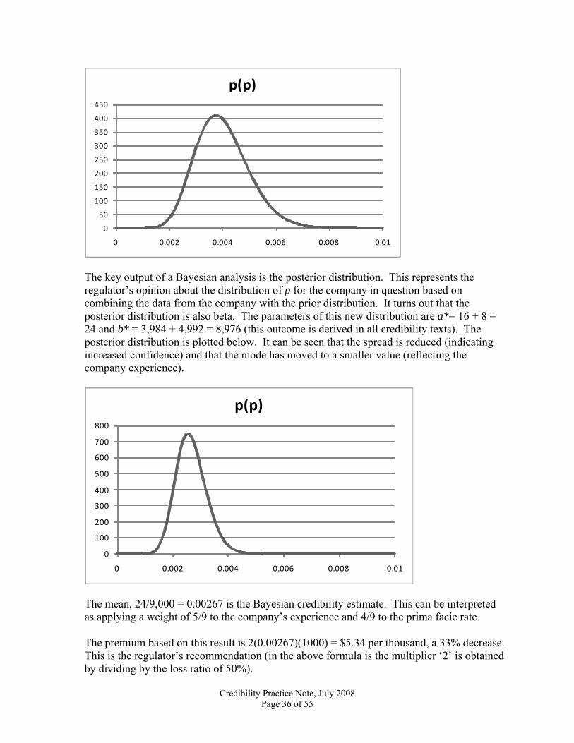
REGULATOR’S CASE The regulator takes a Bayesian approach. Let X denote the number of claims for the company in a given year. It is reasonable to assume that X has a binomial distribution with n = 5,000 and p unknown. The prima facie rate assumes p = 0.004, but individual companies may have different true values of p. In order to use the Bayesian approach, a prior distribution is required. There are two equivalent (in the sense that they lead to the same formulas) interpretations of this distribution. One is that it reflects the regulator’s confidence in the prima facie value of 0.004. The other is that it reflects how the parameter p varies from company to company. The regulator selects a beta distribution with parameters a = 16 and b = 3,984. The beta distribution is selected for two reasons. First, it is easy to work with; all the calculations needed are simple to execute. Second, it has an appropriate shape. Below is a graph of this density function. The parameters were selected so that the mean is the prima facie value of 0.004. The standard deviation of this beta distribution is about 0.001 and this also provides an interpretation of his choice.


0

50

100

150

200

250

300

350

400

450

0 0.002 0.004 0.006 0.008 0.01

p(p)

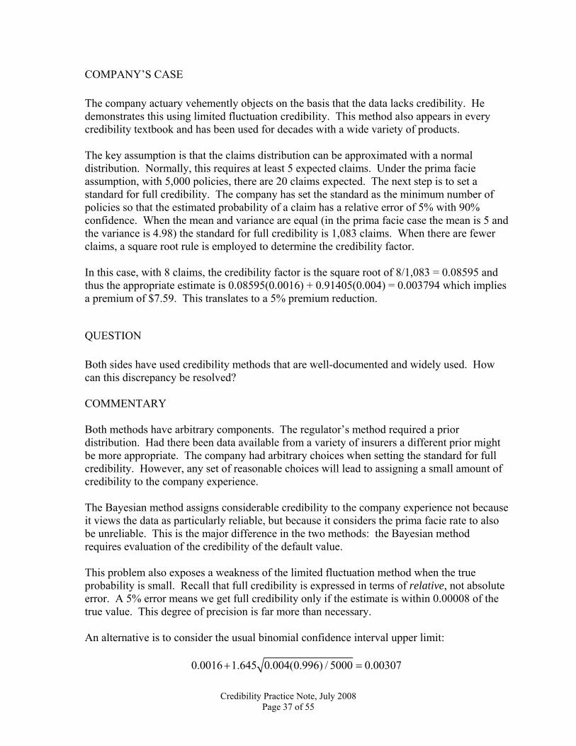
The key output of a Bayesian analysis is the posterior distribution. This represents the regulator’s opinion about the distribution of p for the company in question based on combining the data from the company with the prior distribution. It turns out that the posterior distribution is also beta. The parameters of this new distribution are a*= 16 + 8 = 24 and b* = 3,984 + 4,992 = 8,976 (this outcome is derived in all credibility texts). The posterior distribution is plotted below. It can be seen that the spread is reduced (indicating increased confidence) and that the mode has moved to a smaller value (reflecting the company experience).

0

100

200

300

400

500

600

700

800

0 0.002 0.004 0.006 0.008 0.01

p(p)

The mean, 24/9,000 = 0.00267 is the Bayesian credibility estimate. This can be interpreted as applying a weight of 5/9 to the company’s experience and 4/9 to the prima facie rate. The premium based on this result is 2(0.00267)(1000) = $5.34 per thousand, a 33% decrease. This is the regulator’s recommendation (in the above formula is the multiplier ‘2’ is obtained by dividing by the loss ratio of 50%).


COMPANY’S CASE The company actuary vehemently objects on the basis that the data lacks credibility. He demonstrates this using limited fluctuation credibility. This method also appears in every credibility textbook and has been used for decades with a wide variety of products. The key assumption is that the claims distribution can be approximated with a normal distribution. Normally, this requires at least 5 expected claims. Under the prima facie assumption, with 5,000 policies, there are 20 claims expected. The next step is to set a standard for full credibility. The company has set the standard as the minimum number of policies so that the estimated probability of a claim has a relative error of 5% with 90% confidence. When the mean and variance are equal (in the prima facie case the mean is 5 and the variance is 4.98) the standard for full credibility is 1,083 claims. When there are fewer claims, a square root rule is employed to determine the credibility factor. In this case, with 8 claims, the credibility factor is the square root of 8/1,083 = 0.08595 and thus the appropriate estimate is 0.08595(0.0016) + 0.91405(0.004) = 0.003794 which implies a premium of $7.59. This translates to a 5% premium reduction.

QUESTION Both sides have used credibility methods that are well-documented and widely used. How can this discrepancy be resolved? COMMENTARY Both methods have arbitrary components. The regulator’s method required a prior distribution. Had there been data available from a variety of insurers a different prior might be more appropriate. The company had arbitrary choices when setting the standard for full credibility. However, any set of reasonable choices will lead to assigning a small amount of credibility to the company experience. The Bayesian method assigns considerable credibility to the company experience not because it views the data as particularly reliable, but because it considers the prima facie rate to also be unreliable. This is the major difference in the two methods: the Bayesian method requires evaluation of the credibility of the default value. This problem also exposes a weakness of the limited fluctuation method when the true probability is small. Recall that full credibility is expressed in terms of relative, not absolute error. A 5% error means we get full credibility only if the estimate is within 0.00008 of the true value. This degree of precision is far more than necessary. An alternative is to consider the usual binomial confidence interval upper limit: 0.0016 1.645 0.004(0.996) / 5000 0.00307+ =


which leads to a conservative premium of $6.14, which may be an acceptable compromise. The prior probability was used to provide additional conservativism. One way to reconcile these points of view is until the regulator can gather appropriate data to have confidence in the prior distribution, focus on the one piece of information we have, which is that company’s data and that can be used with the confidence interval approach. Finally, the objectives of the regulator are quite different from those of the company actuary. These differences should be understood in order to assist the actuary with understanding the most appropriate approach used to resolve the given credibility issue.


4. A Short History and Background on Credibility Theory and its Usage in Actuarial Practice

This section draws heavily from the article that Tom Herzog wrote on credibility for the January/February 2008 issue of the Contingencies publication of the Academy. INTRODUCTION Credibility helps determine the weight that the actuary believes should be applied to a particular body of experience in order to estimate future values. It is an example of a statistical estimate. Statistical estimates are obtained through the use of statistical formulas or models which, in turn, are based on statistical approaches or paradigms. There are currently two main approaches or paradigms to statistical inference: (a) the frequentist approach (also called sampling theory or the classical paradigm); and (b) the Bayesian approach. We summarize each of these briefly in the next two sections. FREQUENTIST APPROACH Under the Frequentist Approach, the probability of an event is its relative frequency. Random variables, such as the aggregate claim amount in a period of observation, are assumed to have probability distributions whose parameters are constants. Prior information enters statistical model building only in the selection of a class of models. The main tools used are confidence intervals, unbiased estimates and tests of hypotheses. BAYESIAN APPROACH Under the Bayesian approach, probability is treated as a rational measure of belief. Random variables, such as the aggregate claim amount in a period of observation, are assumed to have probability distributions whose parameters may also have probability distributions. Recent information and prior opinions and/or information (i.e., information available before the recent information) are used to construct the probability distributions of the statistical models or parameters of interest. Thus, the Bayesian approach is based on personal or subjective probabilities and involves the use of Bayes’ theorem. Bayes’ Theorem says that if A and B are events and , then [ ] 0BP >

[ ] [ ] [ ]]B[P

APA|BPB|AP ⋅= (4.1)

This theorem/approach was developed by the Reverend Thomas Bayes. Besides Bayes’ theorem, the main tools of Bayesian statistical inference are predictive distributions, posterior distributions, and (posterior) odds ratios.


Inverse probabilities and statistical inference Bayes’ Theorem is important to actuaries because it enables them to perform statistical inference by computing inverse probabilities. We use the term “inverse” since we infer backwards from results (or effects) to causes. Some simple examples follow. A typical probability problem might be stated as follows: I have a standard die with six sides numbered from “one” through “six” and throw the die three times. What is the probability that the result of each of three tosses of this die will all be a “six”? Now, I might have a second (non-standard) die with three sides numbered “one” and three sides numbered “six”. Again I can ask the same question: What is the probability that the result of each of three tosses of this die will all be a “six”? The idea behind inverse probabilities is to turn the question around. Here, we might observe that the results of three throws of a die were all “sixes.” We then ask the question: What is the probability that we threw the standard die (as opposed to the non-standard die), given these results? Predictive Distributions In insurance work, we typically experience a number of claims or an aggregate amount of losses in one or more prior observation periods. Given these results we want to answer the following questions: (1) How many claims will we experience during the next observation period? (2) What will be the aggregate loss amount during the next observation period? Using Bayes’ Theorem, we can construct an entire probability distribution for such future claim frequencies or loss amounts. Probability distributions of this type are called predictive distributions. Predictive distributions give the actuary much more information than would an average or other summary statistic. A predictive distribution provides the actuary with much more information than just the expected aggregate amount of losses in the next period. For example, it provides the actuary with a complete profile of the tail of the probability distribution of aggregate losses as one might be concerned with in a “value-at-risk” analysis. Thus, predictive distributions can provide the actuary and her client an important tool with which to make business decisions under uncertainty. BASIC CREDIBILITY CONCEPTS Under some approaches to credibility, a compromise estimator, C, is calculated as

( )HZ1ZRC −+= (4.2) where R is the mean of the current observations (for example the data), H is the prior mean (for example, an estimate based on the actuary’s prior data and/or opinion), and Z is the


credibility factor, satisfying the condition .1Z0 ≤≤ The credibility factor, Z, is the weight assigned to the (current) data; (1-Z) is the weight assigned to the prior data. As an insurance example, a new premium rate, C, is derived as a weighted average of an old premium rate, H, and a premium rate, R, whose calculation is based solely on observations from a recent period. An alternative interpretation is to let C be the premium rate for a class of business, to let R be the premium rate whose calculation is based solely on the recent experience of that class, and to let H be the insurance rate whose computation takes into account the recent experience of all classes combined. The credibility factor, Z, is typically of the form

knnZ+

= (4.3)

where and n is a measure of exposure size. Under such a formulation, the problem becomes how to determine k.

0k >

Over the years there have been three major approaches to credibility: Limited Fluctuation, Greatest Accuracy and Bayesian. The Limited Fluctuation Approach and the Greatest Accuracy Approach fall in the frequentist category of approaches. The Greatest Accuracy Approach is also called the Buhlmann Approach, after Hans Buhlmann. Limited Fluctuation Approach to Credibility The Limited Fluctuation Approach seeks to calculate a compromise estimate, C, of the form found in

( )HZ1ZRC −+= . (4.2) The limited fluctuation approach is one of the oldest, going back at least as far as Mowbray’s 1914 paper and Perryman’s 1932 paper. More modern treatments, including complete mathematical derivations, are found in Longley-Cook’s 1962 article and Chapter 5 of Herzog’s 1999 textbook. Outside of North America this approach is sometimes referred to as “American Credibility.” The main advantage of the limited fluctuation approach is that it is relatively simple to use. However, a number of researchers/practitioners have raised questions about the limited fluctuation approach to credibility. Hans Buhlmann, as reported in Hickman and Heacock [1999], felt that the mathematical reasoning behind the limited fluctuation approach as presented by Longley-Cook was “not convincing.” Buhlmann noted that the approach: 1. Was under the frequentist paradigm of statistics and so ignored prior data. 2. Began by deriving the minimum volume of risks required for full credibility.


3. Relied on a derivation that was performed using a confidence interval. 4. Used a standard deviation argument to go from the full credibility requirement to partial

credibility for a smaller volume of risks. Buhlmann raised the following concern with Longley-Cook’s derivation: Why should a confidence interval that, by definition, includes the true value with a probability of less than one, guarantee full credibility? Others have asked why the same weight, 1-Z, is given to the prior mean, H, regardless of the analyst’s view of the accuracy of H. Also, in the case of full credibility, no weight is given to the prior mean, H, as all of the weight is given to the observed data, R. This raises the philosophical question of whether it makes sense to talk about full (i.e., 100%) credibility because more data can generally be obtained. Some analysts believe that no data are entitled to full credibility, so that the credibility curve should approach 1 asymptotically, without ever reaching it. Finally, according to Sundt [1991], there is an internal inconsistency in the limited fluctuation approach to full credibility. He notes that the criterion for replacing the old premium rate is based on the assumption that the old premium rate is correct. This leads to the following conundrum: if the old premium is correct, then why replace it? Buhlmann Approach (Greatest Accuracy Credibility) The credibility estimates produced by Buhlmann’s approach are the best linear approximations to the corresponding Bayesian point estimates. Under this approach, the estimated parameters of the linear model are those that minimize the sum of squared differences between the linear model and the observations. Because Buhlmann’s approach typically 1. requires less mathematical skill, 2. requires fewer computational resources, and 3. does not require the selection of a prior distribution, which can sometimes require

difficult judgments, Buhlmann’s approach to producing point estimates is often much more computationally tractable than a complete Bayesian approach. Bayesian Approach Whitney [1918] stated that the credibility factor, Z, needed to be of the form

knnZ+

= (4.3)

where n represents “earned premiums” and k is a constant to be determined. The problem was how to determine k. Whitney noted that, “In practice k must be determined by judgment.” Specifically, the actuary needs to select the prior probabilities – i.e., the prior


distribution. Whitney also noted that, “The detailed solution to this problem depends upon the use of inverse probabilities” via Bayes’ Theorem. Thoughts on the Choice of a Prior Distribution Buhlmann expressed strong support for the Bayesian paradigm, but felt that whenever possible the prior should be based on experience data rather than on subjective judgment. To quote Buhlmann, as reported in Hickman and Heacox, “Whereas early Bayesian statisticians used the prior distribution of risk parameters as a means to express judgment (which in insurance we would call underwriting judgment), [I] think of the probability distribution of the risk parameters as having an objective meaning. It hence needs to be extracted from the data gathered about the collective. (Only in the case of a lack of such data might one accept the subjective view faute de mieux.) For this reason, I have always insisted on speaking about the structural distribution of risk parameters, avoiding the standard Bayesian terminology, ‘prior distribution’.” Fortunately, as Enrique de Alba points out (in his discussion of a paper by Udi Makov [2001]) “actuarial science is a field where very frequently one has considerable prior information, be it in the form of global or industry-wide information (experience) or in the form of tables.” Because there is so much “objective” prior information available to the actuary, de Alba is surprised that practicing actuaries have not made more extensive use of Bayesian methods. Bayesian Approach and Modern Computing With the increased power of 21st-century computing equipment, advances in statistical algorithms (e.g., the EM algorithm and Markov chain Monte Carlo methods) to implement the Bayesian approach, and widely-available software that performs Bayesian inference (i.e., WinBUGS5), a wider class of problems is becoming susceptible to solution via the Bayesian approach. Another Approach Panel data, also known as longitudinal data, models are regression-type models that have been applied widely in the biological and social sciences. Frees, Young, and Luo [1999] show that many credibility models can be considered special cases of the longitudinal data model. As a consequence, widely-available statistical software that has been produced to analyze longitudinal data can be used to construct credibility models as well. Frees, Young,

5 The BUGS (Bayesian inference Using Gibbs Sampling) Project (begun by the MRC Biostatistics unit at Imperial College, London) is concerned with the development of flexible software for Bayesian analysis of complex statistical models using Markov chain Monte Carlo methods. The “Win” prefix refers to Microsoft’s windows. For details see David Skollnik’s 2001 paper “Actuarial Modeling with MCMC and BUGS”.


and Luo [2001] have a number of examples that illustrate such applications to actuarial problems.


5. Appendices

5.1 Bibliography of Recommended Reading on the Subject of Credibility Theory and Related Approaches

5.2 Regulatory Guidance


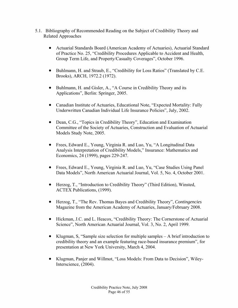
5.1. Bibliography of Recommended Reading on the Subject of Credibility Theory and Related Approaches

• Actuarial Standards Board (American Academy of Actuaries), Actuarial Standard

of Practice No. 25, “Credibility Procedures Applicable to Accident and Health, Group Term Life, and Property/Casualty Coverages”, October 1996.

• Buhlmann, H. and Straub, E., “Credibility for Loss Ratios” (Translated by C.E.

Brooks), ARCH, 1972.2 (1972).

• Buhlmann, H. and Gisler, A., “A Course in Credibility Theory and its Applications”, Berlin: Springer, 2005.

• Canadian Institute of Actuaries, Educational Note, “Expected Mortality: Fully

Underwritten Canadian Individual Life Insurance Policies”, July, 2002.

• Dean, C.G., “Topics in Credibility Theory”, Education and Examination Committee of the Society of Actuaries, Construction and Evaluation of Actuarial Models Study Note, 2005.

• Frees, Edward E., Young, Virginia R. and Luo, Yu, “A Longitudinal Data

Analysis Interpretation of Credibility Models,” Insurance: Mathematics and Economics, 24 (1999), pages 229-247.

• Frees, Edward E., Young, Virginia R. and Luo, Yu, “Case Studies Using Panel

Data Models”, North American Actuarial Journal, Vol. 5, No. 4, October 2001.

• Herzog, T., “Introduction to Credibility Theory” (Third Edition), Winsted, ACTEX Publications, (1999).

• Herzog, T., “The Rev. Thomas Bayes and Credibility Theory”, Contingencies

Magazine from the American Academy of Actuaries, January/February 2008.

• Hickman, J.C. and L. Heacox, “Credibility Theory: The Cornerstone of Actuarial Science”, North American Actuarial Journal, Vol. 3, No. 2, April 1999.

• Klugman, S, “Sample size selection for multiple samples – A brief introduction to

credibility theory and an example featuring race-based insurance premium”, for presentation at New York University, March 4, 2004.

• Klugman, Panjer and Willmot, “Loss Models: From Data to Decision”, Wiley-

Interscience, (2004).


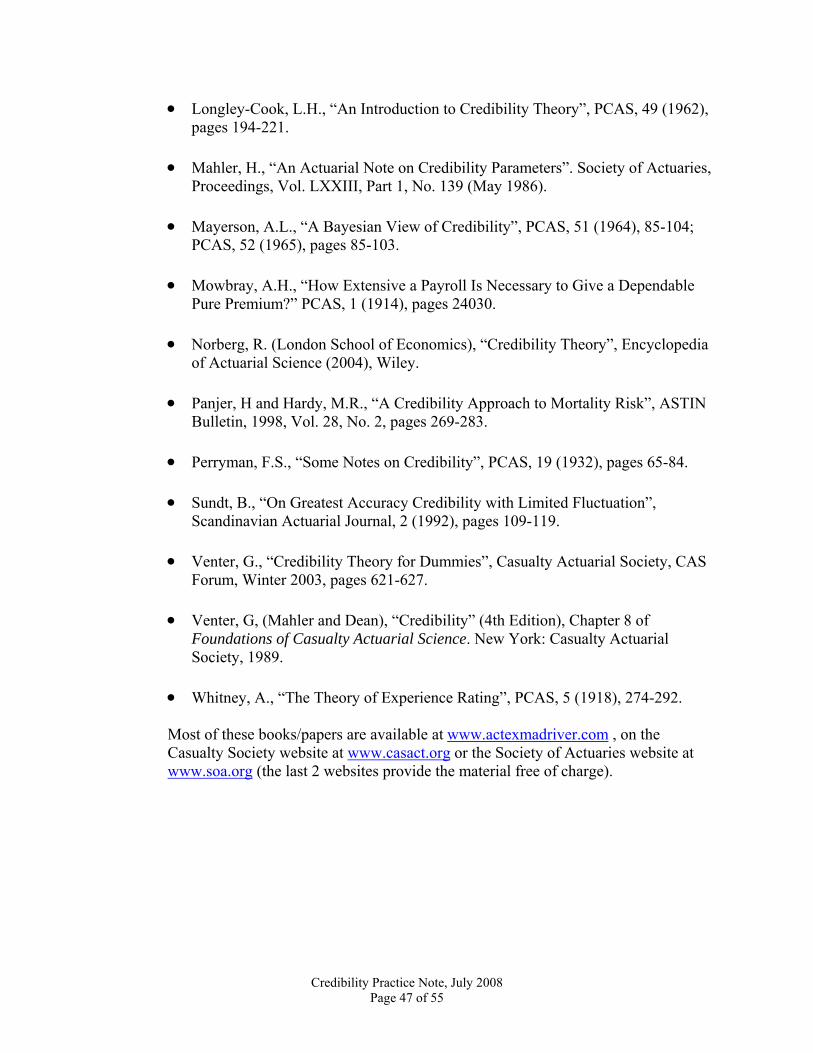
• Longley-Cook, L.H., “An Introduction to Credibility Theory”, PCAS, 49 (1962), pages 194-221.

• Mahler, H., “An Actuarial Note on Credibility Parameters”. Society of Actuaries,

Proceedings, Vol. LXXIII, Part 1, No. 139 (May 1986).

• Mayerson, A.L., “A Bayesian View of Credibility”, PCAS, 51 (1964), 85-104; PCAS, 52 (1965), pages 85-103.

• Mowbray, A.H., “How Extensive a Payroll Is Necessary to Give a Dependable

Pure Premium?” PCAS, 1 (1914), pages 24030.

• Norberg, R. (London School of Economics), “Credibility Theory”, Encyclopedia of Actuarial Science (2004), Wiley.

• Panjer, H and Hardy, M.R., “A Credibility Approach to Mortality Risk”, ASTIN

Bulletin, 1998, Vol. 28, No. 2, pages 269-283.

• Perryman, F.S., “Some Notes on Credibility”, PCAS, 19 (1932), pages 65-84.

• Sundt, B., “On Greatest Accuracy Credibility with Limited Fluctuation”, Scandinavian Actuarial Journal, 2 (1992), pages 109-119.

• Venter, G., “Credibility Theory for Dummies”, Casualty Actuarial Society, CAS

Forum, Winter 2003, pages 621-627.

• Venter, G, (Mahler and Dean), “Credibility” (4th Edition), Chapter 8 of Foundations of Casualty Actuarial Science. New York: Casualty Actuarial Society, 1989.

• Whitney, A., “The Theory of Experience Rating”, PCAS, 5 (1918), 274-292.

Most of these books/papers are available at www.actexmadriver.com , on the Casualty Society website at www.casact.org or the Society of Actuaries website at www.soa.org (the last 2 websites provide the material free of charge).


http://www.actexmadriver.com/

http://www.casact.org/

http://www.soa.org/

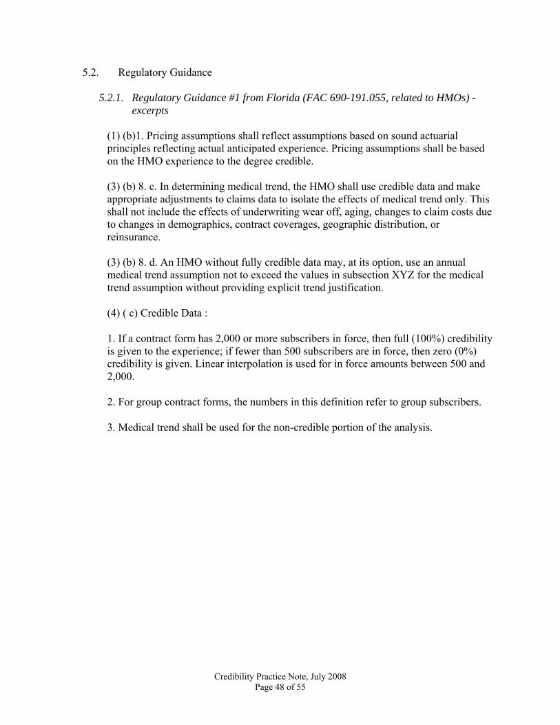
5.2. Regulatory Guidance

5.2.1. Regulatory Guidance #1 from Florida (FAC 690-191.055, related to HMOs) - excerpts

(1) (b)1. Pricing assumptions shall reflect assumptions based on sound actuarial principles reflecting actual anticipated experience. Pricing assumptions shall be based on the HMO experience to the degree credible.

(3) (b) 8. c. In determining medical trend, the HMO shall use credible data and make appropriate adjustments to claims data to isolate the effects of medical trend only. This shall not include the effects of underwriting wear off, aging, changes to claim costs due to changes in demographics, contract coverages, geographic distribution, or reinsurance. (3) (b) 8. d. An HMO without fully credible data may, at its option, use an annual medical trend assumption not to exceed the values in subsection XYZ for the medical trend assumption without providing explicit trend justification.

(4) ( c) Credible Data :

1. If a contract form has 2,000 or more subscribers in force, then full (100%) credibility is given to the experience; if fewer than 500 subscribers are in force, then zero (0%) credibility is given. Linear interpolation is used for in force amounts between 500 and 2,000.

2. For group contract forms, the numbers in this definition refer to group subscribers.

3. Medical trend shall be used for the non-credible portion of the analysis.


5.2.2. Regulatory Guidance #2 from Colorado (3 CCR 702-4, Section 6, related to Rate Filings and Annual Reports for Health Insurance) - excerpts

Section 6. Credibility: The State standard for fully credible data is 2,000 life years and 2,000 claims a year. Both standards must be met within a maximum of three years, if the proposed rates are based on claims experience. 1. The memorandum must discuss the credibility of the State data with the proposed

rates based upon as much State data as possible. The memorandum must also identify and discuss the source, applicability and use of collateral data used to support partially credible State data. The use of collateral data is only acceptable if the State data does not meet the full credibility standard. The formula for determining the amount of credibility to assign to the data is SQRT{(#life years or claims)/full credibility standard}. The full credibility standard is defined above.

2. The memorandum should also discuss how and if the aggregated data meets the

State credibility requirement. Any filing, which bases its conclusions on partially credible data, should include a discussion as to how the rating methodology was modified for the partially credible data.


5.2.3. Regulatory Guidance #3 from North Carolina (11 NCAC 16.0401) – Credit Life Accident and Health Rate Deviation – excerpts

(3) " Case " means either a "Single Account Case" or a "Multiple Account Case" as follows:

(a) " Single Account Case " means an account that is at least 25% credible or, at the option of the insurer, any higher percentage as determined by the Credibility Formula as defined in Item (6) of this Rule; and

(b) " Multiple Account Case " means two or more accounts of the same plan of insurance and class of business having similar underwriting characteristics, excluding single account cases defined in Sub-item (3)(a) of this Rule, and which, when combined, are at least as credible as the minimum level of credibility elected in Sub-item (3)(a) of this Rule.

(5) " Credibility Factor " means the degree to which the past experience of a case can be expected to occur in the future.

(6) " Credibility Formula " means the following process used to calculate the credibility factor:

(a) Determine the incurred claim count during the experience period;

(b) Divide Sub-item (6)(a) of this Rule by 1082;

(c) Take the square root of Sub-item (6)(b) of this Rule; and

(d) The credibility factor is the lesser of the number one and the results of Sub-item (6)(c) of this Rule.


5.2.4. Regulatory Guidance #4 from Texas (28 TAC s 3.3307) – Minimum Standards for Medicare Supplement Policies – excerpts

(d) (2) (E) (i) This rate change and demonstration shall be based on the experience of the named form in this State only, if that experience is fully credible as set out in paragraph (3) of this subsection.

(ii) The rate change and demonstration shall be based on experience of the named form nationwide, with credibility factors as set out in paragraph (3) of this subsection applied, if the named form is used nationwide and the experience in this State is not fully credible.

(iii) The rate change and demonstration shall be based on experience of the named form in this State only, with credibility factors as set out in paragraph (3) of this subsection applied, if the named form is used in this State only and this State’s experience is not fully credible.

(3) For purposes of this subsection, if a group or individual policy form has 2,000 or more policies in force, then full credibility (100%) shall be given to the experience. If fewer than 500 policies are in force, then no credibility (0%) shall be given to the experience. The principle of linear interpolation shall be used for in-force numbers between 500 and 2,000. For group policy forms, the reference in this paragraph to the number of in-force policies means the number of in-force certificates under group policies. For purposes of this section, " in force " means either the average number of policies in force for the experience period used to support the need for a rate revision, or the number of policies in force as of the ending date of the experience period used to support the need for a rate revision. Once an issuer makes a decision as to which definition it will apply to a particular policy form, such decision is irrevocable. An issuer may submit specific alternate credibility standards to the department for consideration. In order for an alternate standard of credibility to be acceptable for application, the issuer must demonstrate that the standards are based on sound actuarial principles, and that the resulting loss ratios are in substantial compliance with the requirements of subsections (a),(b) and (c) of this section.


5.2.5. Regulatory Guidance #5 from California (Title 10, Chapter 5, subchapter 2, Article 6.8) – excerpts

TEST FOR DEVIATED RATES

(a) An insurer shall use life insurance rates and disability insurance rates lower than the prima facie rates for an experience group if the credibility adjusted loss ratio for that group is equal to or less than the Presumptive Loss Ratio (PLR) less .05.

(b) An insurer may use life insurance rates and disability insurance rates higher than the prima facie rates for an experience group when the credibility adjusted loss ratio for that group equals or exceeds PLR + .05.

(c) For application of this Section to life insurance and disability insurance, credibility adjusted loss ratios shall be computed according to Section XYZ for the most recent experience period, based upon applicable prima facie rates for the experience group.

CALCULATION OF THE NEW CASE RATE (2) “Experience period” means the most recent period of time for which experience is reported, but not for a period longer than three full years. An experience period shall end on December 31st of each calendar year.

(A) If an experience group develops a Credibility Factor of 1 from TABLE 4 (“Rate Deviation Credibility Table” in Section XYZ) in less than three years, the experience period for that case will be the number of full years needed to attain that Credibility Factor.

(B) An insurer may elect a level of credibility within the range of TABLE 4 for an experience group. If an experience group develops the minimum credibility elected by the insurer in less than three years, the experience period for that group may be, at the option of the insurer, either the number of full years needed to develop the elected minimum credibility or three full years. If an experience group fails to attain such minimum credibility within three full years, the credibility actually attained in that period shall be used for determining downward deviated rates. Experience incurred in the period immediately preceding the effective date of this regulation may be used to the extent necessary to fill out the experience period.

(4) “Average Number of Life Years” (c) For life insurance and for disability insurance, calculate the credibility adjusted loss ratio(“CLR”) for the experience group using the following formula, where ALR is the actual loss ratio for the experience group on the prima facie rate basis.

CLR = Z(ALR) + PLR(1-Z)

Calculate the new case rate (“NCR”) for the experience group according to the formulas below, where PFR is the prima facie rate for the experience group.

(1) Where CLR is equal to or less than PLR less .05, the downward deviated rate may not exceed the new case rate(“NCR”) calculated as:


NCR = PFR [1 - (PLR-CLR)]

(2) Where CLR exceeds PLR + .05, the upward deviated rate may not exceed the new case rate (“NCR”) calculated as:

NCR = PFR [1 + 1.2(CLR-PLR)]

TABLES

TABLE 4 RATE DEVIATION CREDIBILITY TABLE

Average Number of Life Years

Credibility Factor

(“Z”) Life Disability

(all plans)

Incurred Claim Count

14 Day 30 Day 1 1 1 1 .00

1800 141 209 9 .25 2400 188 279 12 .30 3000 234 349 15 .35 4600 359 535 23 .45 5600 438 651 28 .50 6600 516 767 33 .55 7600 594 884 38 .60 9600 750 1116 48 .65 11600 906 1349 58 .70 14600 1141 1698 73 .75 17600 1375 2047 88 .80 20600 1609 2395 103 .85 25600 2000 2977 128 .90 30600 2391 3558 153 .95 40000 3125 4651 200 1.00

The above integers represent the lower end of the bracket for each “Z” factor. The upper end is 1 less than the lower end for the next higher “Z” factor.


5.2.6. Regulatory Guidance #6 from Maine (rule 220) – excerpts on Credit Life and Health Insurance for one state

(1) The total deviated rate for a specified plan of benefits shall be the appropriate promulgated prima facie premium rate increased or decreased by the additional rate produced by the following formula:

Credibility Factor x (Actual/Expected Ratio - 1) x Prima Facie Claim Cost

(2) A case meets minimum credibility standards if the credibility factor from the

table below is at least equal to the minimum credibility factor elected by the insurer. An insurer may make this election by notice to the Superintendent, in writing. The minimum credibility factor elected may not be less than 50 percent. Once elected, the minimum credibility factor will remain in effect for the insurer until a different factor has been filed by the insurer and approved by the Superintendent. If an insurer makes no written election, its minimum credibility factor will be 100 percent.

(3) The credibility factor may be based on either the Number of Claims incurred or

on the Number of Life Years for the case during the experience period. The insurer shall notify the Superintendent in writing which method it will use to measure the credibility of all its cases in this State and may not change its method without prior approval. If Claim Count or Life Year data is not available, reasonable methods of approximation approved by the Superintendent may be used until such data is developed.


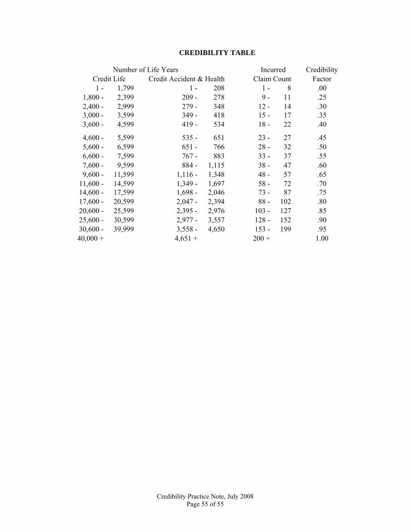
CREDIBILITY TABLE

Number of Life Years Incurred Credibility Credit Life Credit Accident & Health Claim Count Factor

1 - 1,799 1 - 208 1 - 8 .00 1,800 - 2,399 209 - 278 9 - 11 .25 2,400 - 2,999 279 - 348 12 - 14 .30 3,000 - 3,599 349 - 418 15 - 17 .35 3,600 - 4,599 419 - 534 18 - 22 .40

4,600 - 5,599 535 - 651 23 - 27 .45 5,600 - 6,599 651 - 766 28 - 32 .50 6,600 - 7,599 767 - 883 33 - 37 .55 7,600 - 9,599 884 - 1,115 38 - 47 .60 9,600 - 11,599 1,116 - 1,348 48 - 57 .65

11,600 - 14,599 1,349 - 1,697 58 - 72 .70 14,600 - 17,599 1,698 - 2,046 73 - 87 .75 17,600 - 20,599 2,047 - 2,394 88 - 102 .80 20,600 - 25,599 2,395 - 2,976 103 - 127 .85 25,600 - 30,599 2,977 - 3,557 128 - 152 .90 30,600 - 39,999 3,558 - 4,650 153 - 199 .95 40,000 + 4,651 + 200 + 1.00


Documents

A Public Policy PrActice Note - American Academy of Actuaries