A Quasi-IRR for a Project without IRR · PDF file22/11/2014 · A Quasi-IRR for a Project without IRR Flavio Pressacco1 ... NPV ¦a v An internal rate of return (respectively, an internal

1

A Quasi-IRR for a Project without IRR

Flavio Pressacco1

Carlo Alberto Magni2

Patrizia Stucchi3

Abstract

Discounted cash flows methods such as Net Present Value and Internal Rate

of Return are often used interchangeably or even together for assessing value creation

in industrial and engineering projects. Notwithstanding its difficulties of applicability

and reliability, the internal rate of return (IRR) is commonly used in real-life

applications. Among other problems, a project may have no real-valued IRR, a

circumstance that may occur in projects which require shutting costs or imply an

initial positive cash flow such as a down payment made by a client. This paper

supplies a genuine IRR for a project which has no IRR. This seemingly paradoxical

result is achieved by making use of a new approach to rate of return (Magni, 2010),

whereby any project is associated with a unique return function which maps aggregate

capitals into rates of return. Each rate of return is a weighted average of one-period

(internal) rates of return, so it is called Average Internal Rate of Return (AIRR). We

introduce a twin project which has a unique IRR and the same NPV as the original

project's, and which is obtained through an appropriate minimization of the distance

between the original project's cash flow stream and the twin project's. Given that the

latter's IRR lies on the original project's return function, it represents an AIRR of the

original project. And while it is not the IRR of the project, the measure presented is

'almost' the IRR of the project, so it is actually the "quasi-IRR" of the project.

Keywords: Investment analysis, average internal rate of return (AIRR), net present

value, return function, outstanding capital.

JEL Classification: C0, E22, G11, G31.

1 Department of Economics and Statistics – University of Udine.

Email: [email protected] 2 Department of Economics - CEFIN - Center for Research in Banking and Finance -

University of Modena and Reggio Emilia - Email: [email protected] 3 Department of Economics and Statistics – University of Udine.

Email: [email protected]

mailto:[email protected]



F. Pressacco, C.A. Magni, P. Stucchi – A Quasi-IRR for a Project without IRR –

Frontiers in Finance and Economics – Vol 11 N°2, 1-23

2

1 - Introduction

The net present value (NPV) and the internal rate of return (IRR),

both conceived in the 1930s (Fisher, 1930; Boulding, 1935), are arguably the

most widely used investment criteria in real-life applications (Remer and

Nyeto, 1995a, 1995b; Graham and Harvey, 2001). However, in most cases,

managers do not rely on one single investment criterion: NPV and IRR are

often used together, as well as other criteria such as payback, residual income

(e.g., EVA), return on investment, payback period (Remer et al., 1993; Lefely,

1996; Lindblom and Sjögren, 2009). The reason why IRR is widely used in

any economic domain is that a relative measure of economic profitability (a

percentage return) is easily understood, and is more intuitive than an absolute

measure of worth (Evans and Forbes, 1993).

Differences between NPV and IRR have been recognized long since

and have been debated in the literature extensively from various perspectives.

In recent years, scholars have shown a renewed interest in this important

issue. In particular, Hazen (2003) supplies an NPV-compatible decision

criterion for both real-valued and complex-valued IRRs by associating their

real parts with the real parts of the capital streams, so shedding new lights on

the multiple-IRR problem. This problem is tackled by Hartman and Schafrick

(2004) as well, who partition the graph of the NPV function in loaning part

and borrowing part, so singling out the "relevant rate of return". Bosch,

Montllor-Serrats and Tarrazon (2007) use payback coefficients to derive a

normalized index compatible with the NPV, while Kierulff (2008) endorses

the use of the Modified Internal Rate of Return. Osborne (2010) explicitly

links all the IRRs (complex and real) to the NPV and Pierru (2010) gives

complex rates a significant economic meaning. Percoco and Borgonovo

(2012), using sensitivity analysis, focus on the key drivers of value creation

and show that IRR and NPV provide different results. Ben-Horin and Kroll

(2012) suggest that the multiple-IRR problem has limited relevance in

practice.

Evidently, evaluators cannot rest upon a (real) IRR if the polynomial

associated with the project's cash flows has no real roots. A necessary

condition for this to occur is that the project's terminal cash flow has the same



3

sign as the first cash flow. Some engineering projects can actually present

patterns of cash flows which result in negative cash flows in the last part of

the project's life: an investment that requires the removal of equipment or

cleansing of a site in order to return it to its previous state (e.g., a nuclear

plant) may have no real IRR. A similar situation occurs in natural-resource

extractions (mining for coal, gold, ore, silver) where remediation and cleanup

costs are common (see Hartman, 2007). Another situation is the case where a

down payment is made by a client before an investment is made (e.g.,

production on commission).

This paper aims to supply an IRR even in those cases where an IRR

does not exist. This seemingly paradoxical result is obtained by making use of

a new paradigm of rate of return, named Average Internal Rate of Return

(Magni, 2010, 2013). This approach is based on the finding that a project is

uniquely associated (not with a return rate but) with a return function, which

maps invested capitals to (real-valued) average rates of return. Any capital-

rate pair lying on the return function's graph captures the project's economic

profitability: no problem of existence arises and compatibility with NPV in

every circumstance is ensured. Each value taken on by the function is a rate of

return and is called Average Internal Rate of Return (AIRR). Any IRR is

absorbed into the AIRR approach, for it is but a particular case of AIRR,

implicitly associated with a capital automatically computed (in other words,

the IRR lies on the return function).

This paper makes use of the AIRR approach to retrieve the IRR even

in the case where an IRR does not exist. To achieve this objective, we

introduce a twin project, which is a project characterized by three properties:

(a) it has the same length and the same NPV as the project under

consideration, (b) it has a unique real-valued IRR, (c) the distance of its cash

flows stream from the project's cash flow stream is properly minimized. The

latter property means that the twin project is the project which is the closest

one to the original project. To show that such a rate correctly captures the

project's economic profitability, we exploit Magni's (2010, 2013) results to

show that this rate is just a value taken on by the original project's return

function; in other words, it is an AIRR of the project. And given that it is the

internal rate of return of the project which is 'as close as possible' to the

original project, such a measure deserves the name of "quasi-IRR" of the



4

project.

The structure of the paper is as follows. Section 1 presents the main

definitions. Section 2 summarizes the AIRR approach. Section 3 introduces

the minimization procedure necessary to obtain the quasi-IRR, which is the

the IRR of the twin project which is closest to the original project. Section 4

shows that the quasi-IRR is just a particular case of AIRR. Two examples and

some concluding remarks end the paper.

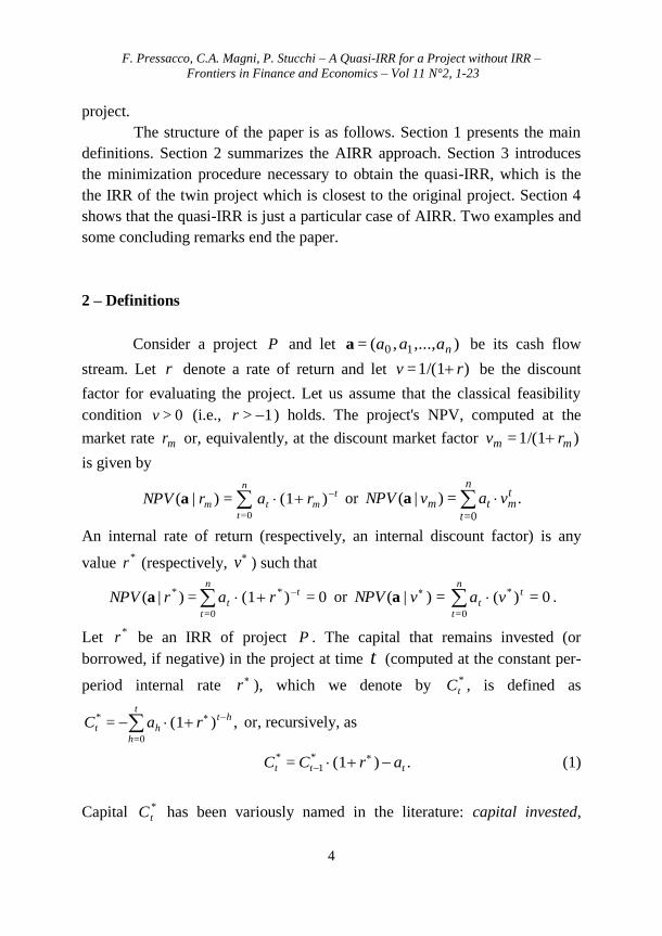
2 – Definitions

Consider a project P and let ),...,,(= 10 naaaa be its cash flow

stream. Let r denote a rate of return and let )1/(1= rv be the discount

factor for evaluating the project. Let us assume that the classical feasibility

condition 0>v (i.e., 1> r ) holds. The project's NPV, computed at the

market rate mr or, equivalently, at the discount market factor )1/(1= mm rv

is given by

tmt

n

tm rarNPV )(1=)|(

0=

a or .=)|(0=

tmt

n

tm vavNPV a

An internal rate of return (respectively, an internal discount factor) is any

value *r (respectively,

v ) such that

0=)(1=)|( *

0=

* tt

n

t

rarNPV a or =)|( vNPV a tt

n

t

va )( *

0=

0= .

Let *r be an IRR of project P . The capital that remains invested (or

borrowed, if negative) in the project at time t (computed at the constant per-

period internal rate r ), which we denote by *

tC , is defined as

,)(1=0=

* hth

t

ht raC or, recursively, as

.)(1= *1

*ttt arCC

(1)

Capital *tC has been variously named in the literature: capital invested,



5

unrecovered balance, unrecovered investment, outstanding capital,

unrecovered investment balance (see Magni, 2009). We also make use of the

symbol ),,,(= **1

*0 nCCC *

C to denote the capital stream implicitly

determined by the internal rate of return *r . The relation this capital stream

bears to the project NPV passes through an excess-return term

)(= *1 mtt rrCG , nt ,1,2,= . which is obtained by the application of an

excess return rate )( mrr to the beginning-of-period outstanding capital.

The NPV may be expressed as the present value, at the market rate, of the

sum of the single period margins:

t

mmt

n

t

t

mt

n

tm vrrCvGvNPV

)(==)|( *

11=1=

a (1)

(see Edwards and Bell, 1961; Peasnell, 1982; Peccati, 1989; Lohmann, 1988;

Pressacco and Stucchi, 1997).

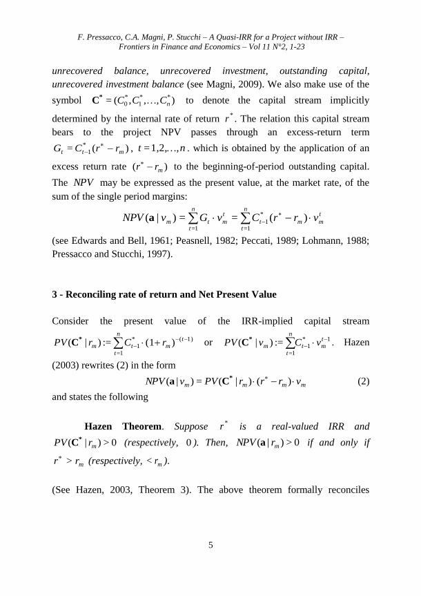
3 - Reconciling rate of return and Net Present Value

Consider the present value of the IRR-implied capital stream

1)(*1

1=

)(1:=) |(

tmt

n

tm rCrPV *

C or 1*1

1=

:=) |(

tmt

n

tm vCvPV *

C . Hazen

(2003) rewrites (2) in the form

mmmm vrrrPVvNPV )() |(=) |( *Ca (2)

and states the following

Hazen Theorem. Suppose *r is a real-valued IRR and

0>) |( mrPV *C (respectively, 0 ). Then, 0>)|( mrNPV a if and only if

mrr > (respectively, mr< ).

(See Hazen, 2003, Theorem 3). The above theorem formally reconciles



6

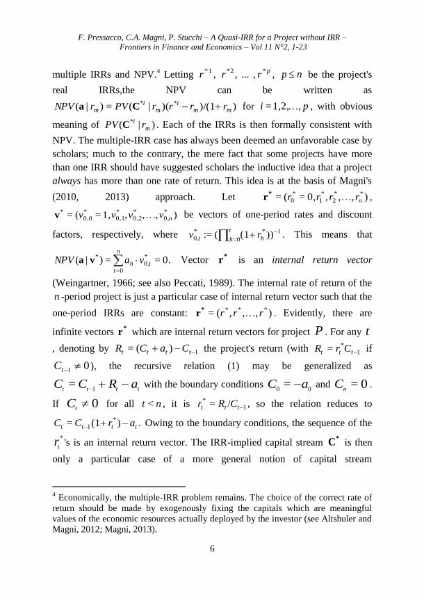
multiple IRRs and NPV.4 Letting

*1r , *2r , ... ,

pr*, np be the project's

real IRRs,the NPV can be written as

))/(1)( |(=)|( **mm

im

im rrrrPVrNPV Ca for pi ,1,2,= , with obvious

meaning of ) |( *m

i rPV C . Each of the IRRs is then formally consistent with

NPV. The multiple-IRR case has always been deemed an unfavorable case by

scholars; much to the contrary, the mere fact that some projects have more

than one IRR should have suggested scholars the inductive idea that a project

always has more than one rate of return. This idea is at the basis of Magni's

(2010, 2013) approach. Let ),,,0,=(= **2

*1

*0 nrrrr *

r ,

),,,1,=(= *0,

*0,2

*0,1

*0,0

*nvvvv v be vectors of one-period rates and discount

factors, respectively, where 1*

0=

*0, ))(1(:= h

t

ht rv . This means that

0.==)|( *0,

0=

*th

n

t

vaNPV va Vector *

r is an internal return vector

(Weingartner, 1966; see also Peccati, 1989). The internal rate of return of the

n -period project is just a particular case of internal return vector such that the

one-period IRRs are constant: ),,,(= *** rrr *r . Evidently, there are

infinite vectors *

r which are internal return vectors for project P . For any t

, denoting by 1)(= tttt CaCR the project's return (with 1*= ttt CrR if

01 tC ), the recursive relation (1) may be generalized as

ttttaRCC

1= with the boundary conditions

00= aC and 0=

nC .

If 0t

C for all nt < , it is 1* /= ttt CRr , so the relation reduces to

.)(1= *1 tttt arCC Owing to the boundary conditions, the sequence of the

*

tr 's is an internal return vector. The IRR-implied capital stream

*C is then

only a particular case of a more general notion of capital stream

4 Economically, the multiple-IRR problem remains. The choice of the correct rate of

return should be made by exogenously fixing the capitals which are meaningful

values of the economic resources actually deployed by the investor (see Altshuler and

Magni, 2012; Magni, 2013).



7

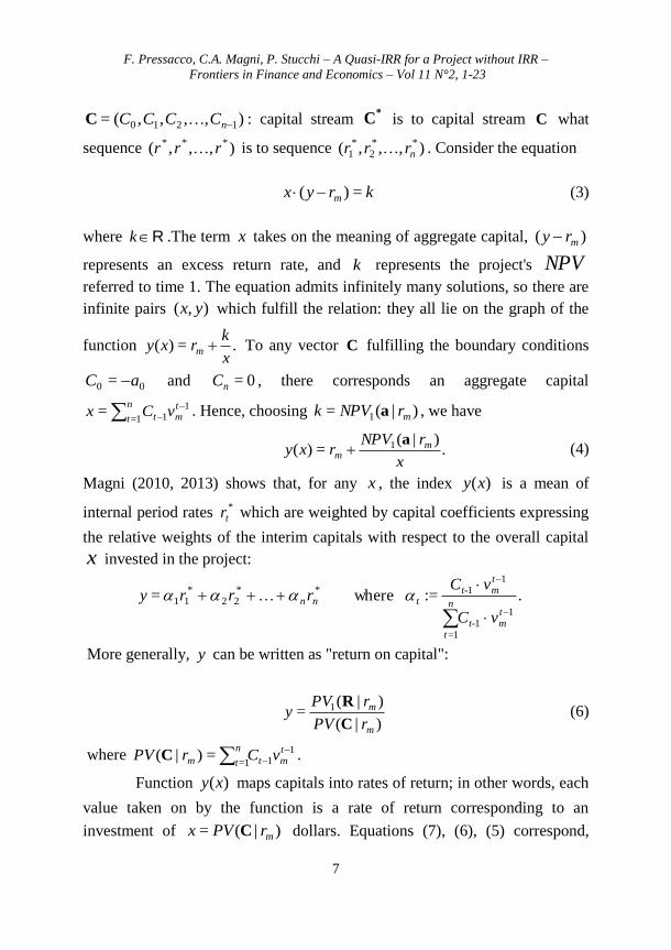
),,,,(= 1210 nCCCC C : capital stream *

C is to capital stream C what

sequence ),,,( *** rrr is to sequence ),,,( **2

*1 nrrr . Consider the equation

kryx m =)( (3)

where Rk .The term x takes on the meaning of aggregate capital, )( mry

represents an excess return rate, and k represents the project's NPV

referred to time 1. The equation admits infinitely many solutions, so there are

infinite pairs ),( yx which fulfill the relation: they all lie on the graph of the

function .=)(x

krxy m To any vector C fulfilling the boundary conditions

00 = aC and 0=nC , there corresponds an aggregate capital

111=

=

tmt

n

tvCx . Hence, choosing )|(= 1 mrNPVk a , we have

.)|(

=)( 1

x

rNPVrxy m

m

a (4)

Magni (2010, 2013) shows that, for any x , the index )(xy is a mean of

internal period rates *tr which are weighted by capital coefficients expressing

the relative weights of the interim capitals with respect to the overall capital

x invested in the project:

.:=where=1

11=

11**

22*

11

tmt-

n

t

tmt-

tnn

vC

vCrrry (5)

More generally, y can be written as "return on capital":

)|(

)|(= 1

m

m

rPV

rPVy

C

R (6)

where 111=

=)|(

tmt

n

tm vCrPV C .

Function )(xy maps capitals into rates of return; in other words, each

value taken on by the function is a rate of return corresponding to an

investment of )|(= mrPVx C dollars. Equations (7), (6), (5) correspond,



8

respectively, to economic intuitions (i), (ii), and (iii) in Magni (2013). Their

common value is called "Average Internal Rate of Return" (AIRR). Any point

),( yx on the graph of )(= xyy represents the univocal association of an

invested capital and its AIRR; the pair )),|(( *rrPV m*

C which identifies the

IRR and its corresponding aggregate capital is only one possible pair among

infinitely many ones.

Magni Theorem. To every project P with cash flow stream

110 ),...,(= n

naaa Ra there corresponds a unique return function

)(= xyy , which maps present values of capital stream to (weighted

average) rates of return. For any capital stream C , consider the aggregate

capital )|(= mrPVx C and let y be the associated rate of return (Average

Internal Rate of Return). Then,

.1

))(|(=)|(

m

mmm

r

ryrPVrNPV

Ca (7)

Furthermore, if 0>)|( mrPV C (respectively, 0< ), then 0>)|( mrNPV a if

and only if mry > , (respectively, mr ).

(See also Magni, 2010, Theorem 2). Hazen Theorem is found back by

choosing any nRC such that )|(=)|( mm rPVrPV *

CC . The return

function )(xy always exists and is uniquely associated to the project,

regardless of whether a real IRR exists or not. And, if an internal rate of return

*r actually exists, the pair )),|(( *rrPV mC is just one point on the curve

)(= xyy (see Magni, 2010, Theorem 3). Any point ))(,( xyx represents the

association of capital invested and return on that capital; depending on which

capital stream is selected, a unique rate of return is derived and the ratio of the

former to the latter captures economic profitability. Furthermore, the above

theorem triggers a general definition of investment (borrowing), which

enables the investor to determine the financial nature of the project on the

basis of empirical evidence.



9

Definition 1. Let C be any fixed capital stream for a project P . Then, a

project is an investment (respectively, borrowing) if 0>) |( mrPV C

(respectively, 0< ). (See Figure 1.)

A project is not uniquely associated with a return rate, but with a

return function (whose values are means of one-period return rates); it is the

capital )|(= rPVx C that is associated with a unique return rate )(xy .

Consider again eq. (4). It may be restated in the following form:

m

mr

yxxrNPV

1

)(1=) |(a (8)

according to which project P is actually turned into a one-period project with

cash flow stream 2))(1,( R yxx and y is its internal rate of return.

Choosing some C , one picks )|(= mrPVx C so that (9) becomes

))(/1)(1|()|(=) |( mmmm ryrPVrPVrNPV CCa .

From a theoretical standpoint, for any fixed choice of mr , project P 's return

function may be derived directly from project P (as shown in section 2)

Therefore, in order to compute a particular rate of return (AIRR), the investor

fixes any x for P : the AIRR (= y ) is then consequently derived. From a

practical standpoint, the most appropriate choice of x is the capital which is

consistent with the value of the economic resources actually employed by the

investor. This choice involves judgmental evaluation (Lindblom and Sjögren,

2009, and Magni, 2013, suggest the use of economic values). However, the

AIRR approach comes to rescue of those evaluators who prefer to have an

IRR, even if an IRR does not exist. In the next sections, we show that a

significant IRR may actually be computed for a no-IRR project.

4 - Managing projects with no IRR with a quasi-IRR

In the previous section, we have derived a return function. In order to

pick one particular value of P 's return function we consider in this section the

set of all those projects with a unique IRR having the same length and the



10

same NPV as project P 's. Within this set we choose the project P whose

cash flows stream ),,,(= 10 naaa a has the minimum distance from project

P 's cash flow stream. Put it equivalently, we individuate a project P through

an adjustment process of P 's cash flows, to the extent that, leaving the NPV

unvaried, the resulting project has a unique IRR.

We will deal with a project P with no IRR such that there is (at least)

a couple ji, of time indices such that 0<ji aa (so excluding projects

having the cash flows with the same sign).5 We start by dealing with a two-

period project in the following subsection and then give a view to introducing

the general n -period extension.

4.1 - Two-period projects

Let P be a two-period project without feasible IRR and with cash

flows of different sign. This means that P is characterized by a NPV which

may be expressed as acvvavNPV /)(=)|( 20 a with 0ac , 00 v .

6

Project P is represented by a cash flow stream which can be framed as the

product of the last cash flow a and a "normalized" cash flow vector a

, that

5 Projects with cash flows not alternating in sign are interpreted as arbitrage strategies.

There is no IRR for these projects and there is no way of adjusting them without

changing the sign of at least one cash flow. Obviously, the AIRR is always available

as a rate of return, even for such a kind of projects. 6 In detail, the conditions depends on the following reasons: (i) 0>a and no real

v

means to deal with projects having strictly positive NPV for any value of the discount

factor; on the contrary, 0<a implies strictly negative NPV. We choose to examine

in detail the problem with a positive a , but all considerations and theorems may be

extended to the symmetric negative case; (ii) starting now from 0>a , we have three

kinds of zeros, that is: (a) both negative: this characterizes a project having all

positive cash flows, that is an arbitrage strategy (see the previous footnote); (b) one

positive and one negative zero: this situation conflicts with the assumption of IRR

unfeasibility; (c) both positive: again impossible if there are no feasible IRR. This

implies positivity of c (in order to rule out positive zeros); (iii) at this point we need

0>0v , otherwise all the cash flows would be positive, giving again an unacceptable

arbitrage strategy.



11

is, .=,12,/=),2,( 0200

20 a=a

avacvaaavcav We look for a twin

project P with cash flow stream a such that, for a fixed mv the NPV of P

and P are equal (NPV-neutrality): ).|(=)|( mm vNPVvNPV aa In addition

we require that project P has a unique feasible zero 0>v , so that the

behaviour of the NPV twin function is analogous to that of the original NPV

function:

)|(=)(=)/|(=)|( 2 vNPVvvavNPVvNPV aaa

with 0>a . Henceforth, without losing generality, we suppose 0>a , so

that is positive. Note that there are two degrees of freedom in the choice of

and v . We can write the row cash flow vector a in terms of the

unknowns in the following, normalized, way: .=),2,(2

a=a avva

Let mP be the value of the project corresponding to the fixed level mv

(greater than zero with the previous assumptions on )and ca of the market

discount factor: ./)(=)|(=/ 20 acvvvNPVaP mm a

For this fixed mv , the

NPV neutrality condition implies: aPvv mm /=)( 2 . This gives the

following solutions for v (we recall that both and a are positive, so mP

is positive as well):

.<<0=2m

mmm

av

P

a

Pvv

(9)

.>=2m

m

mm

mm

av

P

a

Pv

a

Pv

v

(10)

Note that )(= vv depends on , which means that there is a set of (two-

period) projects with unique IRR having the same NPV as project P 's. Within

this set we choose the project with the feasible which minimizes a proper

measure of distance between the original normalized vector a

and the



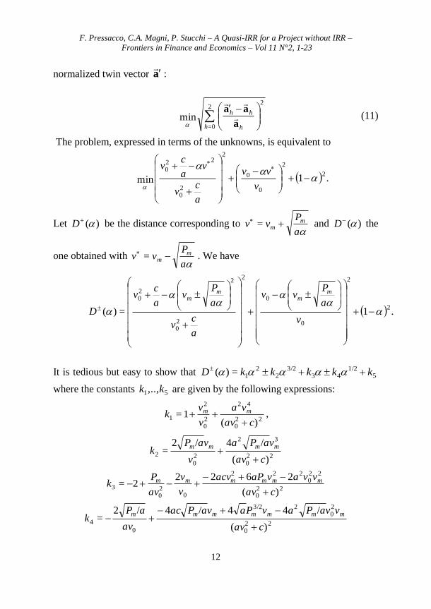
12

normalized twin vector a

:

22

0=

min

h

hh

h a

aa

(11)

The problem, expressed in terms of the unknowns, is equivalent to

.1min2

2

0

0

2

20

220

v

vv

a

cv

va

cv

Let )(D be the distance corresponding to a

Pvv m

m = and )(D the

one obtained with a

Pvv m

m = . We have

.1=)(2

2

0

0

2

20

2

20

v

a

Pvv

a

cv

a

Pv

a

cv

D

mm

mm

It is tedious but easy to show that 51/2

433/2

22

1=)( kkkkkD

where the constants 51,..,kk are given by the following expressions:

220

42

20

2

1)(

1=cav

va

v

vk mm

,

220

32

20

2)(

/4/2=

cav

vaPa

v

vaPk

mmmm

220

220

222

020

3)(

26222=

cav

vvavaPacv

v

v

av

Pk mmmmmm

220

20

23/2

0

4)(

/44/4/2=

cav

vvaPavPavaPac

av

aPk

mmmmmmm



13

220

20

2

5)(

223=

cav

vaPPcPk mmm

.

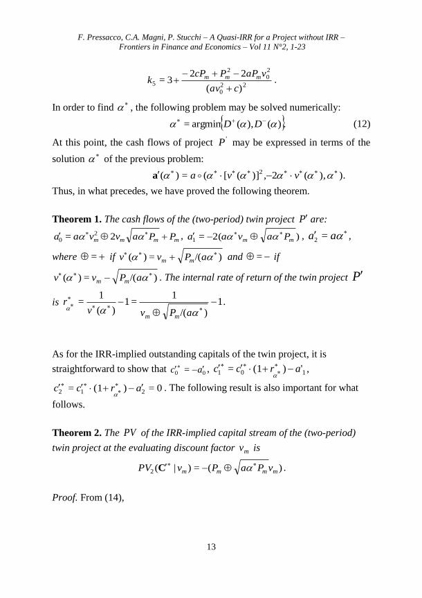
In order to find , the following problem may be solved numerically:

.)(),(argmin= DD (12)

At this point, the cash flows of project 'P may be expressed in terms of the

solution of the previous problem:

).),(2,)]([(=)( 2 vva a (13)

Thus, in what precedes, we have proved the following theorem.

Theorem 1. The cash flows of the (two-period) twin project P are:

mmmm PPavvaa 2= 20

, )2(=1 mm Pavaa , aa =2 ,

where = if )/(=)( aPvv mm and = if

)/(=)( aPvv mm . The internal rate of return of the twin project P

is 1.)/(

1=1

)(

1=

aPvv

r

mm

As for the IRR-implied outstanding capitals of the twin project, it is

straightforward to show that 00 = ac , 101 ')(1= arcc

,

0=)(1= 212 arcc

. The following result is also important for what

follows.

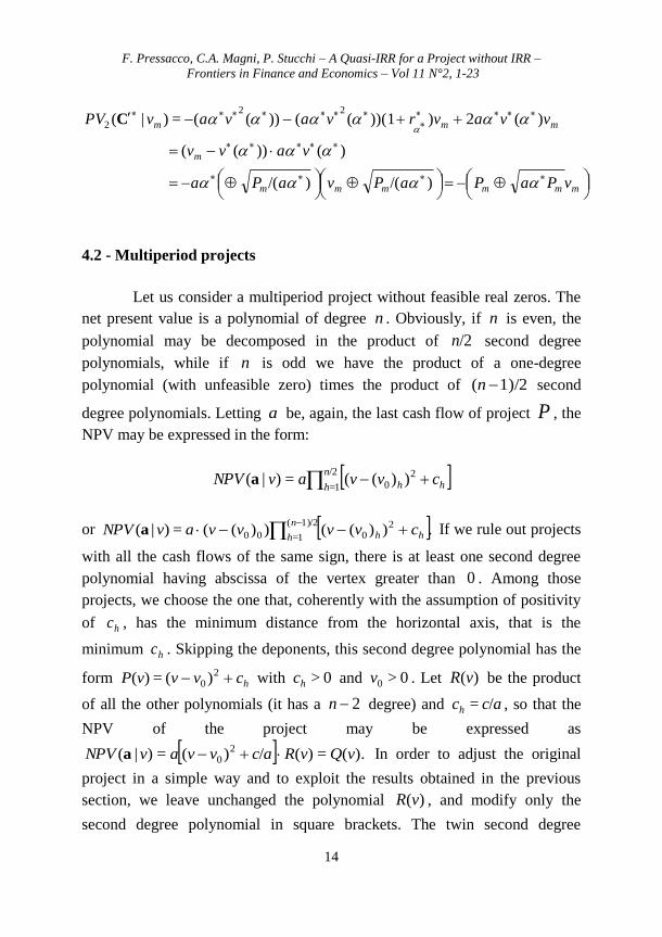
Theorem 2. The PV of the IRR-implied capital stream of the (two-period)

twin project at the evaluating discount factor mv is

)(=) |(2 mmmm vPaPvPV C .

Proof. From (14),



14

mmmmmm

m

mmm

vPaPaPvaPa

vavv

vvavrvavavPV

)/()/(

)())((

)(2)(1))(())((=) |(22

2 C

4.2 - Multiperiod projects

Let us consider a multiperiod project without feasible real zeros. The

net present value is a polynomial of degree n . Obviously, if n is even, the

polynomial may be decomposed in the product of /2n second degree

polynomials, while if n is odd we have the product of a one-degree

polynomial (with unfeasible zero) times the product of 1)/2( n second

degree polynomials. Letting a be, again, the last cash flow of project P , the

NPV may be expressed in the form:

hh

n

hcvvavNPV

20

/2

1=))((=)|(a

or .))(())((=) |( 20

1)/2(

1=00 hh

n

hcvvvvavNPV

a If we rule out projects

with all the cash flows of the same sign, there is at least one second degree

polynomial having abscissa of the vertex greater than 0 . Among those

projects, we choose the one that, coherently with the assumption of positivity

of hc , has the minimum distance from the horizontal axis, that is the

minimum hc . Skipping the deponents, this second degree polynomial has the

form hcvvvP 20 )(=)( with 0>hc and 0>0v . Let )(vR be the product

of all the other polynomials (it has a 2n degree) and acch /= , so that the

NPV of the project may be expressed as

).(=)(/)(=) |( 20 vQvRacvvavNPV a In order to adjust the original

project in a simple way and to exploit the results obtained in the previous

section, we leave unchanged the polynomial )(vR , and modify only the

second degree polynomial in square brackets. The twin second degree



15

polynomial is given by .)(=)( 2 vvvP We let )(vQ be the n-degree twin

polynomial, that is, )()(=)()(=)( 2 vRvvavRvPavQ . As previously

done, we impose NPV neutrality for a fixed mv for the second degree

polynomial, that is: aPacvvvv mmm /=/)(=)( 20

2 . In order to grant

NPV neutrality, for a fixed mv , between projects Q and Q , we extend the

NPV neutrality between the old projects P and 'P . Formally, this means:

).|(=

)(=)(/)(=)(=)(=

)()(=) (=)|(

20

2

m

mmmmmmm

mmmm

vNPV

vQvRacvvavRPvRPa

vRvvavQvNPV

a

a

At this point, we can apply exactly the best fit condition (11) and use (9) and

(10) in order to find and )( v so that the n -period twin project's cash-

flow stream is determined, as well as the (unique) internal rate of return

1)(1/=

vr . As regards the present value of the capital stream of the

project, we show that the following result holds.

Theorem 3. The present value nPV of the IRR-implied outstanding capitals of

the n-period twin project, at the evaluating discount factor mv , is the present

value 2PV of the IRR-implied outstanding capitals of the second degree

polynomial times the NPV of the unmodified, 2)( n degree, polynomial:

).()|(=)|( 2 mmmn vRvPVavPV CC

Proof. We remind (equation (3)) that the present value of the n-period project,

evaluated at the market discount factor mv , may be rewritten in terms of the

present value of the capital stream of the twin project in the following way:

mmmnm vrrvPVvQ )()|(=)( **

C , where *

*r denotes the IRR of the n-

period twin project P . On the other side, for the neutrality condition, we



16

have ).(=)(=)(=)( mmmmmm vRPvRPvQvQ Again, by (3), the present

value of the 2 -period adjusted project is expressed in terms of its IRR-

implied outstanding capitals:

mmmmm vrrvPVavvaP )()|(=)(= **

22

C . Putting these

conditions together, we have

.)()|(=)()()|( **

**

2 mmmnmmmm vrrvPVvRvrrvPVa

CC

Hence, immediately, the conclusion.

5 - The quasi-IRR is a rate of return of the original project

The previous section has introduced the IRR of the twin project,

which we have denoted by **

r . It is the internal rate of return of the project

which is the closest one to P , according to an appropriate measure of

distance. Therefore, it represents the return on each dollar of capital invested

in P , which amounts to ) |( mn rPV *C . In this section, we show that this

measure is not only a rate of return for P , but it is a genuine rate of return

for the original project P as well. Being a rate of return for P and being,

technically, an IRR (of the twin project), we call this rate the "quasi-IRR" of

P . We exploit Magni Theorem, which states that any project P is uniquely

associated with a return function )(= xyy that maps present value of capital

streams to rates of return (AIRR). Let us then consider project P 's return

function and compute the counterimage of the quasi-IRR through )(xy : from

**

* =)(

rxy we have )(= **

1*

ryx and, using (5), one finds

.)|(

=**

1*

m

m

rr

rNPVx

a (14)

Exploiting the NPV-neutrality condition one gets ))/( |(= **1

*mm rrrNPVx

a

Hence,



17

).|(=))(|()(1

=**

***

mn

m

mmmnmrPV

rr

vrrrPVrx *

*

CC

(15)

which shows that the (aggregate) capital invested in project P corresponding

to a rate of return of **

r coincides with the (aggregate) capital invested in the

twin project.

By definition of return function, multiplying the quasi-IRR **

r by *x

one just obtains the corresponding project P 's aggregate return:

.=)|( **

*

rxrPV m *

R Therefore, the quasi-IRR is the ordinate of the point

),( **

*

rx lying on project P 's return function (see Figure 2).

From Magni Theorem and eqs. (15)-(16) the following result

obtains.

Theorem 4. The quasi-IRR correctly captures the economic profitability of

project P . In particular, project P is interpreted as an (aggregate)

investment of *x dollars which generate return at a rate of *

*r . The invested

capital *x coincides with the invested capital )|( mn rPV *

C of the twin

project 'P .

Resting on eq. (9), the information supplied to the investor is then as

follows: project P may be interpreted as a one-period project whose capital

invested is *x and whose internal rate of return is *

** =)(

rxy , which is the

internal rate of return of P . That is, we have kept in with the (seemingly

paradoxical) requirement of computing an internal rate of return which

expresses P 's economic profitability even though P has no internal rate of

return at all.

To sum up, we have found an AIRR for project P representing an

internal rate of return in two senses: (i) it is the (unique) IRR of a project

which strictly resembles project P ; (ii) it is the internal rate of a one-period

project whose outlay coincides with the aggregate capital invested in P .

F. Pressacco, C.A. Magni, P. Stucchi – A Quasi-IRR for a Project without IRR – Frontiers in Finance and Economics – Vol 11 N°2, 1-23

18

Therefore, the rate of return **r does deserve the label of "quasi-IRR" of

project P .

6 - Examples

We will illustrate the meaning of the previous sections through two examples. Let us consider the project P with cash flow vector

14,10)(4.925,=a without real zeros. Its present value may be written in the

form [ ]acvva /)( 20 + with 10=a , 0.7=0v , 0.025=c . Let the market rate

be 0.1=mr (10% ) so that the market discounting factor is 900.=mv and the

NPV, computed at the market rate, is 0.462. The value 1.00875=

(feasible, that is greater than 0.0559=/ 2mm vP ) is the only real solution of the

best fitting problem in (12) and (1.00875)v = 0.695039 , in the form

/10.0875mm Pv , corresponds to a quasi-IRR of 43.8767%=**r , which is

the IRR of the twin project, whose cash flow stream is .0875)14.0224,10(4.87307,=a ; its net present value may be written in the

form 20.695039)10.0875(v , resulting in 0.462 for mvv = (owing to NPV-

neutrality). The return funtion of project P is ;0.5084/0.1=)( xxy + then,

from )(=0.438767 *xy one gets 1.5.=*x The project is (not a borrowing but) an investment and may be interpreted as a one-period investment of 1.5 dollars yielding a 43.8767% internal rate of return. From

/1.1=0.1)|(= 10* CCPVx +C one finds that the interim capital is equal to

7.068=)4.925)(1.1(1.5=1 +C , so that the period rates are

0.4075=114)/4.925(7.068=*1r (borrowing rate) and

0.4148=110)/7.068(0=*2 +r (investment rate), whose weighted mean is

just 0.438767=)/1.51,1(7.068(0.4148)4.925)/1.5((0.4075)= 1+y .

Coming now to a 4 -period project, let us consider project P with

F. Pressacco, C.A. Magni, P. Stucchi – A Quasi-IRR for a Project without IRR – Frontiers in Finance and Economics – Vol 11 N°2, 1-23

19

cash flow stream 336,100)..05,231.49,420(47.477,=a The present value

of P may be framed as [ ] [ ]rr cvvacvva ++ 20

20 )(/)( where the

parameters are 100=a , 0.7=0v , 0.25=c and 0.98=0rv , 0.0036=rc .

Being rcac </ , we let rr cvvvR +20 )(=)( and we proceed as before in

order to adjust the second degree polynomial [ ]acvva /)( 20 + . With

)/(=)( * aPvv mm , we obtain a twin project with cash flow stream

00.8751).337.9395,120.814,230.6885,4(46.9764,=a

The IRR of this project (i.e., the quasi-IRR) is 43.8767%=**r , as before.7

The NPV of the twin project is 0.0399 and project P 's return function is

,0.04387/0.1=)( xxy + whence 0.12949=*x . The project is, again, an investment, and may be interpreted as a one-period investment of 0.12949 dollars yielding a 43.8767% internal rate of return. The interim capitals are found by 0.12949=/1.1/1.1/1.147.477 3

32

21 CCC +++ . Unlike the two-period example, there is not a unique solution. Precisely, there are two degrees of freedom, that is infinite solutions. It may be convenient to choose

0.438767== *2

*1 rr (the quasi-IRR of the project), which implies 163.18=1C

and 185.269=2C . This in turn implies 69.71=3C whence 0.4373=*3r ,

0.4345=*4r . It is then easy to check that the mean of the rates weighted by its

corresponding capitals is just the quasi-IRR. Geometrically, the present value of the twin project as a function of the discount factor v has the graph as in Figure 3, where the dashed curve is the NPV of the original project and the

7

We only use four decimals after the comma, to avoid notational awkwardness. A better approximation of the IRR is found with

(4.873071949177,-14.022433915853, 10.008751024893) (two-period twin project) and

(46.976413590066,-230.688473152691, 420.814023042214, -337.939540037641, 100.8751025) (four-period twin project). Of course, this notational practice (four decimals only) has been applied to all the results in the example.



20

other one is the NPV of the twin project as a function of v .

7 - Concluding remarks

Several classes of projects may have no IRR. While this may occur

rarely, the consequences are serious. The NPV can be still used for assessing

wealth creation, but an important information is missed, that is, the amount of

value created per unit of invested capital. In real life, industrial and

engineering projects may occasionally meet this difficulty. Magni (2010)

introduces a new approach to rate of return, based on the finding that any

project is not associated with a rate of return but with a return function, which

exists and is unique, and which maps aggregate capitals to rates of return,

each of which is called Average Internal Rate of Return (AIRR), being a

weighted average of one-period internal rates of return. He also shows that

any IRR and its associated capital lies on such a return function (i.e., it is a

particular case of AIRR). As any AIRR captures the project's economic

profitability, there is the need of singling out the appropriate capital, which

expresses the economic resources that are actually employed in the investment

(i.e., one point on the graph of the return function). The choice should be

made on the basis of sound economic reasoning and empirical evidence

(Magni, 2013). Notwithstanding the flaws of the IRR, many investors are very

familiar with IRR and privilege it as an intuitive relative measure of worth. In

this paper, we show that the AIRR approach can come to the rescue of the

IRR even when the IRR does not exist. To require an IRR whenever no IRR

exists seems just to be (contradictory) wishful thinking. The paradox is

overcome by minimizing an appropriate distance between the cash flow

stream of the original project and the cash flows stream of a twin project

which has a unique IRR and has the same NPV of the original project. Hence,

using the return function of the original project, we show that the IRR of the

twin project is an AIRR of the original project, associated with a well-

determined capital. In other words, the IRR of the twin project captures the

economic profitability of the original project, in the sense that it is NPV-

consistent. The project may be interpreted as a one-period investment whose



21

traditional IRR is just the IRR of the twin project. To sum up, the IRR of the

twin project is an AIRR with two compelling features: (i) it is the IRR of the

project whose cash flow stream is the closest one to the original project's; (ii)

it is the IRR of a one-period project with initial outlay coinciding with the

aggregate capital invested in the project. While not exactly the IRR of the

project, the IRR of the twin project is almost the IRR of the project: it is the

project's 'quasi-IRR'. Such a metric is NPV-consistent and overcomes the

classical IRR problems in accept/reject decisions and choice between

competing projects (to this end, incremental quasi-IRR can be computed).

References

Altshuler, D., Magni, C.A. 2012. Why IRR is not the rate of return for your

investment: Introducing AIRR to the real estate community. The

Journal of Real Estate Portfolio Management, 18(2), 219–230.

Ben-Horin, M., Kroll, Y., 2012. The limited relevance of the multiple IRRs.

The Engineering Economist, 57, 101–118.

Bodenhorn, D. 1964. A Cash-flow concept of profit. Journal of Finance

(March), 19(1), 16–31.

Bosch, M.T., Montllor-Serrats, J., Tarrazon, M.A. 2007. NPV as a function of

the IRR: The value drivers of investment projection, Journal of

Applied Finance 17 (Fall/Winter), 41–45.

Boulding, K.E. 1935. The theory of the single investment. Quarterly Journal

of Economics, 49 (May), 475–494.

Edwards, E., Bell, P. 1961. The Theory and Measurement of Business Income.

Berkeley University of California Press.

Evans, D.A, Forbes, S.M. 1993. Decision making and display methods: The

case of prescription and practice in capital budgeting. The

Engineering Economist, 39, 87–92.

Fisher, I. 1930. The Theory of Interest. Clifton: August M. Kelley Publishers.

Gitman, L.J., Forrester, J.R. 1977. A survey of capital budgeting techniques

used by major U.S. firms. Financial Management, 6(3), 66–71.

Hartman, J.C., Schafrick, I.C., 2004. The relevant internal rate of return. The

Engineering Economist, 49, 139–158.



22

Hazen, G.B. 2003. A new perspective on multiple internal rates of return. The

Engineering Economist, 48(1), 31–51.

Hazen, G.B. 2009. An extension of the internal rate of return to stochastic

cash flows. Management Science, 55(6) (June), 1030–1034.

Kierulff, H. 2008. MIRR: A better measure. Business Horizons, 51, 321–329.

Lefley, F., 1996. The payback method of investment appraisal: A review and

synthesis. International Journal of Production Economics, 44, 207–

224.

Lindblom, T., Sjögren, S., 2009. Increasing goal congruence in project

evaluation by introducing a strict market depreciation schedule.

International Journal of Production Economics, 121, 519–532.

Lohmann, J.R. 1988. The IRR, NPV and the fallacy of the reinvestment rate

assumption. The Engineering Economist, 33(4) (Summer), 303–330.

Magni, C.A. 2009. Splitting up value: A critical review of residual income

theories. European Journal of Operational Research, 198(1)

(October), 1–22.

Magni C.A. 2010. Average Internal Rate of Return and investment decisions:

a new perspective. The Engineering Economist, 55(2), 150–181.

Magni, C.A. 2013. The Internal-Rate-of-Return approach and the AIRR

paradigm: A refutation and a corroboration. The Engineering

Economist, 58(2), 73−111.

Osborne, M. 2010. A resolution to the NPV-IRR debate? The Quarterly

Review of Economics and Finance, 50(2) (May), 234−239.

Peasnell, K.V. 1982.] Some formal connections between economic values and

yields and accounting numbers. Journal of Business Finance &

Accounting, 9(3), 361–381.

Peccati, L. 1989. Multiperiod analysis of a levered portfolio. Decisions in

Economics and Finance, 12(1) (March), 157–166. Reprinted in

J. Spronk & B. Matarazzo (Eds.), 1992, Modelling for Financial

Decisions. Berlin: Springer-Verlag.

Percoco, M., Borgonovo, E., 2012. A note on the sensitivity analysis of the

internal rate of return. International Journal of Production

Economics, 135, 526–529.

Pierru, A. 2010. The simple meaning of complex rates of return. The

Engineering Economist, 55(2), 105–117.



23

Pressacco, F. Stucchi P. 1997. Su una estensione bidimensionale del teorema

di scomposizione di Peccati, [A two-dimensional extension of

Peccati’s decomposition theorem, in Italian], Decisions in Economics

and Finance, 20(199), 169–185.

Remer, D.S., Nieto, A.P., 1995a. A compendium and comparison of 25

project evaluation techniques. Part 1: Net present value and rate of

return methods. International Journal of Production Economics, 42,

79–96.

Remer, D.S., Nieto, A.P., 1995b. A compendium and comparison of 25

project evaluation techniques. Part 2: Ratio, payback, and accounting

methods. International Journal of Production Economics, 42, 101–

129.

Remer, D.S., Stokdyk, S.B., Van Driel, M., 1993. Survey of project

evaluation techniques currently used in industry. International

Journal of Production Economics, 32, 103–115.

Weingartner, H.M. 1966. The generalized rate of return. The Journal of

Financial and Quantitative Analysis, 1(3) (September), 1–29.

Documents

A Quasi-IRR for a Project without IRR · PDF file22/11/2014 · A Quasi-IRR for a Project without IRR Flavio Pressacco1 ... NPV ¦a v An internal rate of return (respectively, an internal