The Astronomical Journal, 138:568–578, 2009 August doi:10.1088/0004-6256/138/2/568C© 2009. The American Astronomical Society. All rights reserved. Printed in the U.S.A.

A SEARCH FOR OCCULTATIONS OF BRIGHT STARS BY SMALL KUIPER BELT OBJECTS USINGMEGACAM ON THE MMT

F. B. Bianco1,2,3

, P. Protopapas2,3

, B. A. McLeod2, C. R. Alcock

2, M. J. Holman

2, and M. J. Lehner

1,2,41 University of Pennsylvania, 209 South 33rd Street, Philadelphia, PA 19104, USA; fbianco@cfa.harvard.edu

2 Harvard-Smithsonian Center for Astrophysics, 60 Garden Street, Cambridge, MA 02138, USA3 Initiative in Innovative Computing at Harvard, 60 Oxford Street, Cambridge, MA 02138, USA

4 Institute of Astronomy and Astrophysics, Academia Sinica, P.O. Box 23-141, Taipei 106, TaiwanReceived 2009 March 17; accepted 2009 May 26; published 2009 July 7

ABSTRACT

We conducted a search for occultations of bright stars by Kuiper Belt Objects (KBOs) to estimate the density ofsubkilometer KBOs in the sky. We report here the first results of this occultation survey of the outer solar systemconducted in 2007 June and 2008 June/July at the MMT Observatory using Megacam, the large MMT optical imager.We used Megacam in a novel shutterless continuous-readout mode to achieve high-precision photometry at 200 Hz,which with point-spread function convolution results in an effective sampling of ∼ 30 Hz. We present an analysis of220 star hours of data at a signal-to-noise ratio of 25 or greater, taken from images of fields within 3◦ of the eclipticplane. The survey efficiency is greater than 10% for occultations by KBOs of diameter d � 0.7 km, and we report nodetections in our data set. We set a new 95% confidence level upper limit for the surface density ΣN (d) of KBOs largerthan 1 km: ΣN (d � 1 km) � 2.0×108 deg−2, and for KBOs larger than 0.7 km ΣN (d � 0.7 km) � 4.8×108 deg−2.

Key words: Kuiper Belt – solar system: formation

1. INTRODUCTION

The size distribution of objects in the Kuiper Belt is believedto be shaped by competitive processes of collisional agglomera-tion and disruption. The details of the structure of the Kuiper Beltsize distribution can reveal information on the internal structureof the Kuiper Belt Objects (KBOs), the history of planet migra-tion (Kenyon & Bromley 2004; Pan & Sari 2005), and the gashistory in the solar system (Kenyon & Bromley 2009). Largesize objects in the Kuiper Belt (diameter d � 30 km, through-out the paper any mention of the size of a KBO will refer toits diameter) can be observed directly in reflected sunlight. Theluminosity distribution for objects larger than 100 km is welldescribed by a single power-law cumulative luminosity distri-bution ΣN (< R) = 10α(R−R0), where ΣN (< R) is the number ofKBOs brighter than magnitude R per degree in the sky on theecliptic plane, with an index α ∼ 0.7 and R0 ∼ 23 (Fraser et al.2008; Fuentes & Holman 2008). This, under the assumption of4% constant albedo, translates into a power-law size distributionn(d) ∝ d−q with power index q ∼ 4.5. For these objects, thesize distribution reflects the history of agglomeration.

There is strong evidence for a break in the slope of the distri-bution at fainter magnitudes (smaller KBO sizes). Constraintson the extrapolation of a single power law to magnitude greaterthan R ∼ 35 were placed by Kenyon & Windhorst (2001), whoinvoked Olbers’s paradox applied to the zodiacal background,and by Stern & McKinnon (2000), who derived a slope forthe distribution of small KBOs of q ≈ 3 on the basis of thecratering on Triton as observed by Voyager 2, though this evi-dence is questioned in Schenk & Zahnle (2002). A further hintof a break in the size distribution of KBOs is offered by thebetter-probed size distribution of Jupiter Family Comets (JFCs;Tancredi, Fernandez, Rickman, & Licandro 2006, and refer-ences therein). These objects are likely injected into their cur-rent orbits from the Kuiper Belt or the scattered disk (Volk &Malhotra 2008, VM hereafter), and it is argued that their sizedistribution would be preserved during this process. The sizedistribution of JFCs is well represented by a shallow slope:

q = 2.7 in the diameter range 1–10 km. Future microwavebackground surveys may also allow the setting of constraints onthe mass, distance, and size distribution of outer solar system(OSS) objects (Babich et al. 2007).

Bernstein et al. (2004) conducted a deep Hubble SpaceTelescope (HST) survey with the Advanced Camera for Surveys(ACS) which led to the detection of three KBOs of magnitudeR > 26.5; an extrapolation of the bright end power law wouldhave predicted a factor of about 25 more detections for thissurvey. This reveals that a break in the power-law distributionmust occur at magnitude brighter than R = 28.5 (d ∼ 20 km).This work remains the state of the art in deep direct surveys of theOSS, with a completeness of 50% at magnitude R = 28.5. Morerecently, Fuentes et al. (2009) and Fraser & Kavelaars (2009)detected more KBOs in the R � 27 region of the size spectrumand better constrained the slope of the bright end of the powerlaw and the location of the break, R ∼ 25 (d ∼ 50–100 km;Fuentes et al. 2009; Fraser & Kavelaars 2009).

KBOs smaller than about 30 km in diameter still elude directobservations. Occultation surveys are the only observationalmethod presently expected to be able to detect such small objectsin the Kuiper Belt. These surveys monitor background starsawaiting the serendipitous alignment of KBOs with the stars.The transit of a KBO along the line of sight briefly modifies theobserved flux of the target star. At the distance of the KuiperBelt (∼ 40 AU), the size of the objects of interest is close to theFresnel scale for visible light: this causes such occultation eventsto be diffraction-dominated phenomena. The Fresnel scale isdefined as F = √

λD/2 (Born & Wolf 1980; Roques et al.1987), where D is the distance to the occulter and λ is thewavelength at which the occultation is observed. In our survey,the bandpass of the observation is centered near λ = 500 nmand, at distance D ≈ 40 AU, F ≈ 1.2 km. Any occultationcaused by objects in the Kuiper Belt of a few kilometers indiameter or smaller will exhibit prominent diffraction effects. Adiffraction pattern, characterized by an alternation of bright anddark fringes centered on the KBO, translates into a modulatedlight curve during the transit of the KBO along the line of sight.

568

No. 2, 2009 SEARCH FOR OCCULTATIONS OF BRIGHT STARS BY KBOs 5695

km

1 km

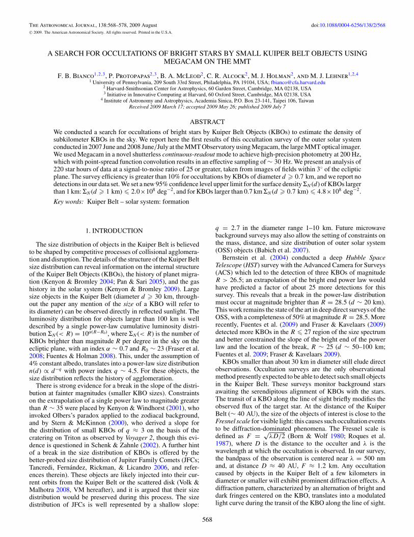
Figure 1. Simulated diffraction pattern (left panel) generated by a sphericald = 1 km KBO occulting a magnitude 12 F0V star. The MMT/Megacamsystem bandpass (Sloan r ′ filter and camera quantum efficiency) is assumed.The size of the KBO and the size of the Airy ring—a measure of the cross sectionof the event—are shown for comparison. The right panel shows the diffractionsignature of the event (assuming central crossing: impact parameter b = 0) asa function of the distance to the point of closest approach (bottom scale). Thetop scale shows the time-line of the event assuming an observation conductedat opposition (relative velocity vrel ≈ 25 km s−1). The occultation is sampledat 200 Hz (dashed line), and at 30 Hz, the effective sampling rate after takingPSF effects into account (solid line, see Section 4).

A unique feature, showing a series of wiggles, and generallya reduction in flux, is imprinted in the time series of the star(Roques & Moncuquet 2000; Nihei et al. 2007; see Figure 1).

The overall flux reduction is dominated by the size of theKBO, while the duration of the event depends upon the relativevelocity vrel and the size of the diffraction pattern H. We defineH as the diameter of the first Airy ring, which it is limited bythe Fresnel scale for subkilometer KBOs and by the size of theobject for large KBOs as follows (Nihei et al. 2007):

H ≈ [(2√

3F )32 + d

32 ]

23 + θ�D, (1)

where the additional Dθ� term accounts for the finite angular sizeof the star. When observing at opposition, the relative velocityvrel of an object orbiting the Sun at 40 AU is about 25 km s−1

and the typical duration of an occultation by subkilometer KBOsis about 0.2 s.

Occultation surveys were first proposed by Bailey (1976),but only recently results have been reported. Chang et al. (2007)conducted a search for KBO occultations in the archival RXTEX-ray observations of Scorpius X-1 (Sco X-1). They reporteda surprisingly high rate of occultation-like phenomena: dips inthe light curves compatible with occultations by objects between10 and 200 m in diameter. Jones et al. (2008) showed that mostof the dips in the Sco X-1 light curves may be attributed toartificial effects of the response of the RXTE photomultiplierafter high-energy events, such as strong cosmic ray showers. Inthe 90 minutes of RXTE data analyzed only 12 of the original58 candidates cannot be ruled out as artifacts, but are hard toconfirm as events (Jones et al. 2008; Chang et al. 2007; Liuet al. 2008). New RXTE/PCA data of Sco X-1 provided a lessconstraining upper limit to the size distribution of KBOs (Liuet al. 2008).

Several groups have conducted occultation surveys in the op-tical regime. Roques et al. (2006, R06 hereafter) and Bickertonet al. (2008, BKW hereafter) independently observed narrowfields at 45 Hz and 40 Hz, respectively, with frame transfercameras. Such cameras allowed them to obtain high signal-to-noise ratio (S/N) fast photometry on two stars simultaneously.Both surveys expect a very low event rate due to the limited

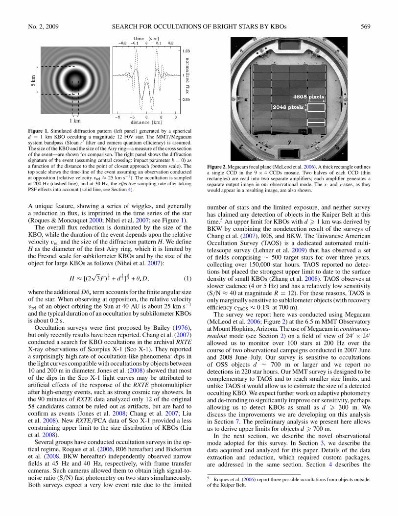
Figure 2. Megacam focal plane (McLeod et al. 2006). A thick rectangle outlinesa single CCD in the 9 × 4 CCDs mosaic. Two halves of each CCD (thinrectangles) are read into two separate amplifiers; each amplifier generates aseparate output image in our observational mode. The x- and y-axes, as theywould appear in a resulting image, are also shown.

number of stars and the limited exposure, and neither surveyhas claimed any detection of objects in the Kuiper Belt at thistime.5 An upper limit for KBOs with d � 1 km was derived byBKW by combining the nondetection result of the surveys ofChang et al. (2007), R06, and BKW. The Taiwanese AmericanOccultation Survey (TAOS) is a dedicated automated multi-telescope survey (Lehner et al. 2009) that has observed a setof fields comprising ∼ 500 target stars for over three years,collecting over 150,000 star hours. TAOS reported no detec-tions but placed the strongest upper limit to date to the surfacedensity of small KBOs (Zhang et al. 2008). TAOS observes atslower cadence (4 or 5 Hz) and has a relatively low sensitivity(S/N ≈ 40 at magnitude R = 12). For these reasons, TAOS isonly marginally sensitive to subkilometer objects (with recoveryefficiency εTAOS ≈ 0.1% at 700 m).

The survey we report here was conducted using Megacam(McLeod et al. 2006; Figure 2) at the 6.5 m MMT Observatoryat Mount Hopkins, Arizona. The use of Megacam in continuous-readout mode (see Section 2) on a field of view of 24′ × 24′allowed us to monitor over 100 stars at 200 Hz over thecourse of two observational campaigns conducted in 2007 Juneand 2008 June–July. Our survey is sensitive to occultationsof OSS objects d ∼ 700 m or larger and we report nodetections in 220 star hours. Our MMT survey is designed to becomplementary to TAOS and to reach smaller size limits, andunlike TAOS it would allow us to estimate the size of a detectedocculting KBO. We expect further work on adaptive photometryand de-trending to significantly improve our sensitivity, perhapsallowing us to detect KBOs as small as d � 300 m. Wediscuss the improvements we are developing on this analysisin Section 7. The preliminary analysis we present here allowsus to derive upper limits for objects d � 700 m.

In the next section, we describe the novel observationalmode adopted for this survey. In Section 3, we describe thedata acquired and analyzed for this paper. Details of the dataextraction and reduction, which required custom packages,are addressed in the same section. Section 4 describes the

5 Roques et al. (2006) report three possible occultations from objects outsideof the Kuiper Belt.

570 BIANCO ET AL. Vol. 138

characteristics of the noise of our current data sets, and ournoise mitigation approach. Section 5 describes the detectionalgorithm. In Section 6, we derive our upper limit to the densityof KBOs. We also compare in detail the achievements of oursurvey to those of previous surveys. We draw our conclusionsand outline future work in Section 7.

2. FAST PREPHOTOMETRY WITH A LARGETELESCOPE: THE CONTINUOUS-READOUT MODE

Achieving subsecond photometric sampling is a challenge inoptical astronomy. CCD cameras can perform fast photometricobservations by reading out small subimages, limiting theobservations to very small portions of the sky (e.g., Marsh& Dhillon 2006). This is the approach adopted by R06 andBKW, who observed two stars at one time. Due to the rarityof occultation events, however, one would want to maximizethe number of targets and the total exposure to increase thenumber of detections. TAOS achieves subsecond photometricobservation on up to 500 targets with the zipper mode readouttechnique (Lehner et al. 2009), but they sample at � 5 Hzrate. Our continuous-readout technique allows us to observe theentire field of view of the camera at 200 Hz.

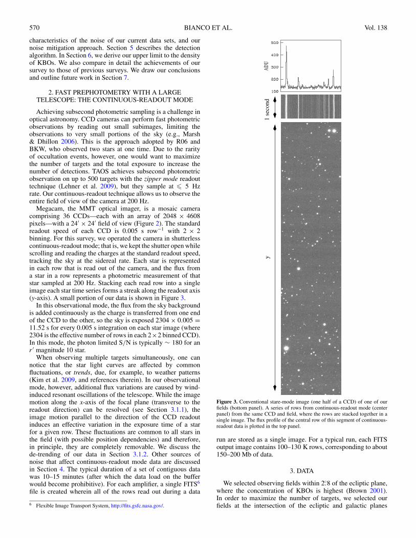
Megacam, the MMT optical imager, is a mosaic cameracomprising 36 CCDs—each with an array of 2048 × 4608pixels—with a 24′ × 24′ field of view (Figure 2). The standardreadout speed of each CCD is 0.005 s row−1 with 2 × 2binning. For this survey, we operated the camera in shutterlesscontinuous-readout mode; that is, we kept the shutter open whilescrolling and reading the charges at the standard readout speed,tracking the sky at the sidereal rate. Each star is representedin each row that is read out of the camera, and the flux froma star in a row represents a photometric measurement of thatstar sampled at 200 Hz. Stacking each read row into a singleimage each star time series forms a streak along the readout axis(y-axis). A small portion of our data is shown in Figure 3.

In this observational mode, the flux from the sky backgroundis added continuously as the charge is transferred from one endof the CCD to the other, so the sky is exposed 2304 × 0.005 =11.52 s for every 0.005 s integration on each star image (where2304 is the effective number of rows in each 2×2 binned CCD).In this mode, the photon limited S/N is typically ∼ 180 for anr ′ magnitude 10 star.

When observing multiple targets simultaneously, one cannotice that the star light curves are affected by commonfluctuations, or trends, due, for example, to weather patterns(Kim et al. 2009, and references therein). In our observationalmode, however, additional flux variations are caused by wind-induced resonant oscillations of the telescope. While the imagemotion along the x-axis of the focal plane (transverse to thereadout direction) can be resolved (see Section 3.1.1), theimage motion parallel to the direction of the CCD readoutinduces an effective variation in the exposure time of a starfor a given row. These fluctuations are common to all stars inthe field (with possible position dependencies) and therefore,in principle, they are completely removable. We discuss thede-trending of our data in Section 3.1.2. Other sources ofnoise that affect continuous-readout mode data are discussedin Section 4. The typical duration of a set of contiguous datawas 10–15 minutes (after which the data load on the bufferwould become prohibitive). For each amplifier, a single FITS6

file is created wherein all of the rows read out during a data

6 Flexible Image Transport System, http://fits.gsfc.nasa.gov/.

1 se

cond

y

Figure 3. Conventional stare-mode image (one half of a CCD) of one of ourfields (bottom panel). A series of rows from continuous-readout mode (centerpanel) from the same CCD and field, where the rows are stacked together in asingle image. The flux profile of the central row of this segment of continuous-readout data is plotted in the top panel.

run are stored as a single image. For a typical run, each FITSoutput image contains 100–130 K rows, corresponding to about150–200 Mb of data.

3. DATA

We selected observing fields within 2.◦8 of the ecliptic plane,where the concentration of KBOs is highest (Brown 2001).In order to maximize the number of targets, we selected ourfields at the intersection of the ecliptic and galactic planes

No. 2, 2009 SEARCH FOR OCCULTATIONS OF BRIGHT STARS BY KBOs 571

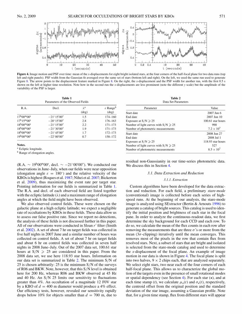
Figure 4. Image motion and PSF over time: mean of the x-displacements for eight bright isolated stars, at the four corners of the half-focal plane for two data runs (topleft and right panels). PSF width from the Gaussian fit averaged over the same set of stars (bottom left and right). On the left, we used the same run used to generateFigure 8. The arrow points to the displacement feature marked in Figure 8. On the right, the x-displacement and the PSF width for another run, with the first 0.5 sshown on the left at higher time resolution. Note how in the second run the x-displacements are less prominent (note the different y scale) but the amplitude of thevariability of the PSF is larger.

Table 1Parameters of the Observed Fields

R.A. Decl. λa ε Rangeb

(deg) (deg)

17h00m00s −21◦15′00′′ 1.5 174–16017h15m00s −20◦15′00′′ 2.8 176–16318h00m00s −21◦15′00′′ 2.2 171–17318h00m00s −21◦30′00′′ 1.9 171–17318h00m00s −21◦45′00′′ 1.7 172–17319h00m00s −22◦00′00′′ 0.7 158–172

Notes.a Ecliptic longitude.b Range of elongation angles.

(R.A. ∼ 19h00m00s, decl. ∼ −21◦00′00′′). We conducted ourobservations in June–July, when our fields were near opposition(elongation angle ε = 180◦) and the relative velocity of theKBOs is highest (Roques et al. 1987; Nihei et al. 2007; Bickertonet al. 2009), thus maximizing the event rate per target star.Pointing information for our fields is summarized in Table 1.The R.A. and decl. of each observed field are listed togetherwith the ecliptic latitude (λ) and a maximum range of elongationangles at which the field might have been observed.

We also observed control fields. These were chosen on thegalactic plane at a high ecliptic latitude; we expect a negligiblerate of occultations by KBOs in these fields. These data allow usto assess our false positive rate. Since we report no detections,the analysis of these fields is not discussed further in this paper.All of our observations were conducted in Sloan r ′ filter (Smithet al. 2002). A set of about 7 hr on target fields was collected infive half nights in 2007 June and a similar number of hours wascollected on control fields. A set of about 7 hr on target fieldsand about 6 hr on control fields was collected in seven halfnights in 2008 June–July. Out of the 2007 data set, 100.61 starhours at S/N � 25 are considered in this paper. From the2008 data set, we use here 118.93 star hours. Information onour data set is summarized in Table 2. The minimum S/N of25 is chosen arbitrarily: 25 is the minimum S/N of the surveysof R06 and BKW. Note, however, that this S/N level is obtainedhere for 200 Hz, whereas R06 and BKW observed at 45 Hzand 40 Hz. An S/N 25 limits our sensitivity to fluctuationsgreater than 4%. An occultation of a magnitude 12 F0V starby a KBO of d = 400 m diameter would produce a 4% effect.Our efficiency tests, however, revealed our sensitivity rapidlydrops below 10% for objects smaller than d = 700 m, due to

Table 2Data Set Parameters

Parameter Value

Start date 2007 Jun 6End date 2007 Jun 10Exposure at S/N � 25 100.61 star hoursNumber of light curves with S/N � 25 990Number of photometric measurements 7.2 × 107

Start date 2008 Jun 27End date 2008 Jul 1Exposure at S/N � 25 118.93 star hoursNumber of light curves with S/N � 25 527Number of photometric measurements 8.5 × 107

residual non-Gaussianity in our time-series photometric data.We discuss this in Section 4.

3.1. Data Extraction and Reduction

3.1.1. Extraction

Custom algorithms have been developed for the data extrac-tion and reduction. For each field, a preliminary stare-mode(conventional) image is collected before each series of high-speed runs. At the beginning of our analysis, the stare-modeimage is analyzed using SExtractor (Bertin & Arnouts 1996) togenerate a catalog of bright sources. This catalog is used to iden-tify the initial position and brightness of each star in the focalpane. In order to analyze the continuous-readout data, we firstdetermine the sky background for each CCD and each row. Todo so, we calculate the mean of the flux counts in each row afterremoving the measurements that are three σ ’s or more from themean (3σ -clipping) iteratively until the mean converges. Thisremoves most of the pixels in the row that contain flux fromresolved stars. Next, a subset of stars that are bright and isolatedis selected from the stare-mode catalog and used to determinethe x-displacement of the focal plane. An example of imagemotion in our data is shown in Figure 4. The focal plane is splitinto two halves, 9 × 2 chips each, that are analyzed separately.We select eight stars, two near each of the four corners of eachhalf-focal plane. This allows us to characterize the global mo-tion of the targets even in the presence of small rotational modesor spatial dependency (see Section 4). For each star (�), and ateach time stamp (t), we calculate μ�(t) and σ�(t), respectively,the centroid offset from the original position and the standarddeviation of the star image, assuming a Gaussian profile. Notethat, for a given time stamp, flux from different stars will appear

572 BIANCO ET AL. Vol. 138

on different rows due to the y-positions of the stars on the focalplane. A one-dimensional Gaussian

F� = I� exp

(− (x − μ�(t))2

2σ 2� (t)

)+ Ibg (2)

(where F� is the total star flux, I� the flux at the peak, and Ibgthe sky) is fitted for each of the eight stars to each row of thestar streak. Thus, the x-displacement μ(t) for all the stars in thefield at time stamp t is estimated to be the weighted average ofthe star displacements

μ(t) =∑N

�=1 ω�(μ�(t) − μ�(t0))∑N�=1 ω�

, (3)

where μ�(t0) is the star initial x-position and ω� is the weightused for that star and N is typically N = 8.

In order to weight our average, we use the correlation of theentire x-displacement time series μ� with respect to the rest ofthe star set:

ω(i, j ) = 1

T

T∑t=0

(μi(t) − 〈μi〉)(μj (t) − 〈μj 〉)s2i (t)s2

j (t), (4)

ω� = 1

N − 1

∑j �=�

ω(�, j ), (5)

where s2 is the variance of the displacement throughout theduration T of the time series. The weight ω� is the square of thePearson’s correlation coefficient (Rice 2006), a measure of thecorrelation of the displacement time series for one star with theother seven. All star light curves in the field are then extractedby aperture photometry adjusting time stamp by time stamp thecenter of the aperture according to the x-motion derived in thisstage, and with a fixed aperture size which is proportional to theaverage FWHM in the run.7

3.1.2. De-Trending

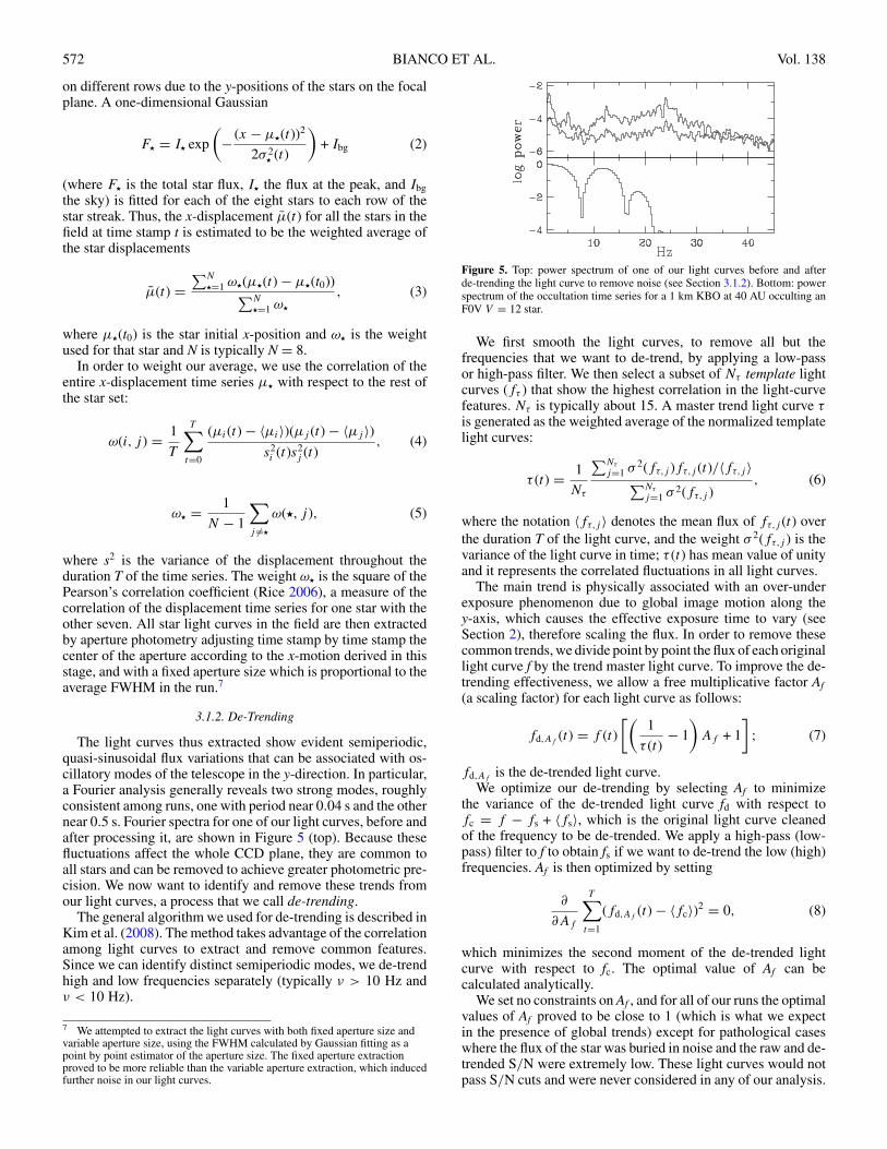
The light curves thus extracted show evident semiperiodic,quasi-sinusoidal flux variations that can be associated with os-cillatory modes of the telescope in the y-direction. In particular,a Fourier analysis generally reveals two strong modes, roughlyconsistent among runs, one with period near 0.04 s and the othernear 0.5 s. Fourier spectra for one of our light curves, before andafter processing it, are shown in Figure 5 (top). Because thesefluctuations affect the whole CCD plane, they are common toall stars and can be removed to achieve greater photometric pre-cision. We now want to identify and remove these trends fromour light curves, a process that we call de-trending.

The general algorithm we used for de-trending is described inKim et al. (2008). The method takes advantage of the correlationamong light curves to extract and remove common features.Since we can identify distinct semiperiodic modes, we de-trendhigh and low frequencies separately (typically ν > 10 Hz andν < 10 Hz).

7 We attempted to extract the light curves with both fixed aperture size andvariable aperture size, using the FWHM calculated by Gaussian fitting as apoint by point estimator of the aperture size. The fixed aperture extractionproved to be more reliable than the variable aperture extraction, which inducedfurther noise in our light curves.

Figure 5. Top: power spectrum of one of our light curves before and afterde-trending the light curve to remove noise (see Section 3.1.2). Bottom: powerspectrum of the occultation time series for a 1 km KBO at 40 AU occulting anF0V V = 12 star.

We first smooth the light curves, to remove all but thefrequencies that we want to de-trend, by applying a low-passor high-pass filter. We then select a subset of Nτ template lightcurves (fτ ) that show the highest correlation in the light-curvefeatures. Nτ is typically about 15. A master trend light curve τis generated as the weighted average of the normalized templatelight curves:

τ (t) = 1

Nτ

∑Nτ

j=1 σ 2(fτ,j )fτ,j (t)/〈fτ,j 〉∑Nτ

j=1 σ 2(fτ,j ), (6)

where the notation 〈fτ,j 〉 denotes the mean flux of fτ,j (t) overthe duration T of the light curve, and the weight σ 2(fτ,j ) is thevariance of the light curve in time; τ (t) has mean value of unityand it represents the correlated fluctuations in all light curves.

The main trend is physically associated with an over-underexposure phenomenon due to global image motion along they-axis, which causes the effective exposure time to vary (seeSection 2), therefore scaling the flux. In order to remove thesecommon trends, we divide point by point the flux of each originallight curve f by the trend master light curve. To improve the de-trending effectiveness, we allow a free multiplicative factor Af(a scaling factor) for each light curve as follows:

fd,Af(t) = f (t)

[(1

τ (t)− 1

)Af + 1

]; (7)

fd,Afis the de-trended light curve.

We optimize our de-trending by selecting Af to minimizethe variance of the de-trended light curve fd with respect tofc = f − fs + 〈fs〉, which is the original light curve cleanedof the frequency to be de-trended. We apply a high-pass (low-pass) filter to f to obtain fs if we want to de-trend the low (high)frequencies. Af is then optimized by setting

∂

∂Af

T∑t=1

(fd,Af(t) − 〈fc〉)2 = 0, (8)

which minimizes the second moment of the de-trended lightcurve with respect to fc. The optimal value of Af can becalculated analytically.

We set no constraints on Af , and for all of our runs the optimalvalues of Af proved to be close to 1 (which is what we expectin the presence of global trends) except for pathological caseswhere the flux of the star was buried in noise and the raw and de-trended S/N were extremely low. These light curves would notpass S/N cuts and were never considered in any of our analysis.

No. 2, 2009 SEARCH FOR OCCULTATIONS OF BRIGHT STARS BY KBOs 573

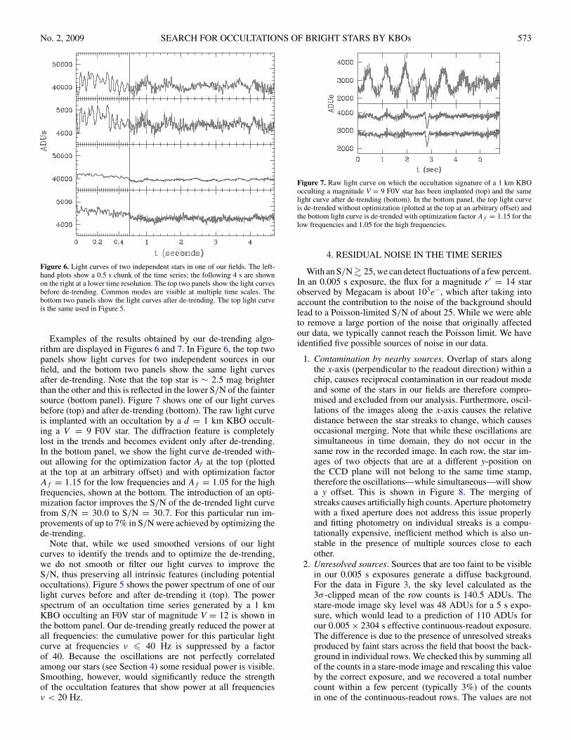
Figure 6. Light curves of two independent stars in one of our fields. The left-hand plots show a 0.5 s chunk of the time series; the following 4 s are shownon the right at a lower time resolution. The top two panels show the light curvesbefore de-trending. Common modes are visible at multiple time scales. Thebottom two panels show the light curves after de-trending. The top light curveis the same used in Figure 5.

Examples of the results obtained by our de-trending algo-rithm are displayed in Figures 6 and 7. In Figure 6, the top twopanels show light curves for two independent sources in ourfield, and the bottom two panels show the same light curvesafter de-trending. Note that the top star is ∼ 2.5 mag brighterthan the other and this is reflected in the lower S/N of the faintersource (bottom panel). Figure 7 shows one of our light curvesbefore (top) and after de-trending (bottom). The raw light curveis implanted with an occultation by a d = 1 km KBO occult-ing a V = 9 F0V star. The diffraction feature is completelylost in the trends and becomes evident only after de-trending.In the bottom panel, we show the light curve de-trended with-out allowing for the optimization factor Af at the top (plottedat the top at an arbitrary offset) and with optimization factorAf = 1.15 for the low frequencies and Af = 1.05 for the highfrequencies, shown at the bottom. The introduction of an opti-mization factor improves the S/N of the de-trended light curvefrom S/N = 30.0 to S/N = 30.7. For this particular run im-provements of up to 7% in S/N were achieved by optimizing thede-trending.

Note that, while we used smoothed versions of our lightcurves to identify the trends and to optimize the de-trending,we do not smooth or filter our light curves to improve theS/N, thus preserving all intrinsic features (including potentialoccultations). Figure 5 shows the power spectrum of one of ourlight curves before and after de-trending it (top). The powerspectrum of an occultation time series generated by a 1 kmKBO occulting an F0V star of magnitude V = 12 is shown inthe bottom panel. Our de-trending greatly reduced the power atall frequencies: the cumulative power for this particular lightcurve at frequencies ν � 40 Hz is suppressed by a factorof 40. Because the oscillations are not perfectly correlatedamong our stars (see Section 4) some residual power is visible.Smoothing, however, would significantly reduce the strengthof the occultation features that show power at all frequenciesν < 20 Hz.

Figure 7. Raw light curve on which the occultation signature of a 1 km KBOocculting a magnitude V = 9 F0V star has been implanted (top) and the samelight curve after de-trending (bottom). In the bottom panel, the top light curveis de-trended without optimization (plotted at the top at an arbitrary offset) andthe bottom light curve is de-trended with optimization factor Af = 1.15 for thelow frequencies and 1.05 for the high frequencies.

4. RESIDUAL NOISE IN THE TIME SERIES

With an S/N � 25, we can detect fluctuations of a few percent.In an 0.005 s exposure, the flux for a magnitude r ′ = 14 starobserved by Megacam is about 103e−, which after taking intoaccount the contribution to the noise of the background shouldlead to a Poisson-limited S/N of about 25. While we were ableto remove a large portion of the noise that originally affectedour data, we typically cannot reach the Poisson limit. We haveidentified five possible sources of noise in our data.

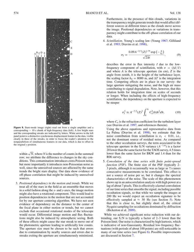
1. Contamination by nearby sources. Overlap of stars alongthe x-axis (perpendicular to the readout direction) within achip, causes reciprocal contamination in our readout modeand some of the stars in our fields are therefore compro-mised and excluded from our analysis. Furthermore, oscil-lations of the images along the x-axis causes the relativedistance between the star streaks to change, which causesoccasional merging. Note that while these oscillations aresimultaneous in time domain, they do not occur in thesame row in the recorded image. In each row, the star im-ages of two objects that are at a different y-position onthe CCD plane will not belong to the same time stamp,therefore the oscillations—while simultaneous—will showa y offset. This is shown in Figure 8. The merging ofstreaks causes artificially high counts. Aperture photometrywith a fixed aperture does not address this issue properlyand fitting photometry on individual streaks is a compu-tationally expensive, inefficient method which is also un-stable in the presence of multiple sources close to eachother.

2. Unresolved sources. Sources that are too faint to be visiblein our 0.005 s exposures generate a diffuse background.For the data in Figure 3, the sky level calculated as the3σ -clipped mean of the row counts is 140.5 ADUs. Thestare-mode image sky level was 48 ADUs for a 5 s expo-sure, which would lead to a prediction of 110 ADUs forour 0.005 × 2304 s effective continuous-readout exposure.The difference is due to the presence of unresolved streaksproduced by faint stars across the field that boost the back-ground in individual rows. We checked this by summing allof the counts in a stare-mode image and rescaling this valueby the correct exposure, and we recovered a total numbercount within a few percent (typically 3%) of the countsin one of the continuous-readout rows. The values are not

574 BIANCO ET AL. Vol. 138

C D EAB

B

A

D

E

C

Figure 8. Stare-mode image (right) read out from a single amplifier and acorresponding ∼ 10 s chunk of high-frequency data (left). A few bright starsand the corresponding streaks are indicated by letters. White arrows in the leftpanel point to a distinctive synchronous displacement feature in the data, visibleclearly in three of the streaks, in order to focus the reader’s attention to thenonparallelism of simultaneous features in our data, which is due to offset inthe original y-position.

within√

N , where N is the number of counts in the summedrow; we attribute the difference to changes in the sky con-ditions. This contamination introduces extra Poisson noise,but more importantly it introduces non-Poissonian noise aswell, since the unresolved sources are affected by the sametrends the bright stars display. Our data show evidence ofoff-phase correlation that might be induced by unresolvedsources.

3. Positional dependency in the motion and trends. While wetreat all of the stars in the field as an ensemble that movesin a solid fashion along the x- and y-axes, the image motionmight also have a rotational component. This would lead toposition dependencies in the motion that are not accountedfor by our aperture centering algorithm. We have not seenevidence of dependency on the distance to the center ofthe focal plane in either motion or trends, but we cannotexclude that occasional rotational modes of the telescopewould occur. Differential image motion and flux fluctua-tions might also be induced by atmospheric seeing. Bothof these effects might cause the star streak to move out ofthe photometric aperture leading to artificially low counts.The aperture size must be chosen to be such that errorsdue to contamination by nearby sources and errors due tostreaks exiting the aperture are simultaneously minimized.

Furthermore, in the presence of thin clouds, variations inthe transparency might generate trends that would affect dif-ferent sources at different times as the clouds move acrossthe image. Positional dependencies or variations in trans-parency might contribute to the off–phase correlation of ourdata.

4. Scintillation. Young’s scaling law (Young 1967; Gillilandet al. 1993; Dravins et al. 1998),

σI =0.09A−2/3(Z)1.75 exp

(− hh0

)√

2Δt, (9)

describes the error in flux intensity I due to the low-frequency component of scintillation, with σ = (ΔI/I )and where A is the telescope aperture (in cm), Z is theangle from zenith, h is the height of the turbulence layer,the scaling factor h0 = 8000 m, and ΔT is the integrationtime. Competing effects are in place in our survey: thelarge aperture mitigating the noise, and the high air masscontributing to signal degradation. Note, however, that thisrelation holds for integration time on scales of secondsor longer. When including the effects of high-frequencyscintillation, the dependency on the aperture is expected tobe steeper

σ 2I ∝ A−7/3(Z)3

∫ ∞

0C2

n(h)h2dh, (10)

where Cn is the refraction coefficient for the turbulent layer(see Dravins et al. 1997, and references therein).Using the above equations and representative data fromLa Palma (Dravins et al. 1998), we estimate that thenoise contribution from scintillation is σI < 0.01, i.e.,not the dominant source of residual noise. As comparedto the other occultation surveys, the term associated to thetelescope aperture in the S/N variance (A−7/6) is a factor20 lower than the same factor for the TAOS survey, 4.5 timeslower than the same factor for BKW and 1.4 than for theR06 survey.

5. Convolution of the time series with finite point-spreadfunction (PSF). The finite size of the PSF (typically 2–3 pixels, although it occasionally was as large as 7) causesconsecutive measurements to be correlated. This effect isnot a source of noise per se, but it changes the spectralcharacteristics of the noise. The scale of this phenomenonshows up in an autocorrelation analysis with high power at alag of about 7 pixels. This is effectively a kernel convolutionof our time series that smooths the signal, including possibleoccultation signals, so that while we sample the images at200 Hz we would expect an occultation signature to beeffectively sampled at ≈ 30 Hz (see Section 5). Notethat this is close to, but slightly short of, the criticalNyquist sampling for occultations dominated by diffraction(Bickerton et al. 2009).

While we achieved significant noise reduction with our de-trending, our S/N is typically a factor of 2–3 lower than thePoisson limit. Our noise is characterized by high kurtosis, whichis indicative of non-Gaussianity. Residual low-frequency fluc-tuations (with periods of about 100 points) are still noticeable inmany of our time series (see Figure 6). Possible improvementsare discussed in Section 7.

No. 2, 2009 SEARCH FOR OCCULTATIONS OF BRIGHT STARS BY KBOs 575

5. SEARCH FOR EVENTS AND EFFICIENCY

5.1. Detection Algorithm

The signature of an occultation, sampled at any rate � 20 Hz,is very distinctive: it shows several fluctuations prior to the Airyring peak, then a deep trough and possibly a Poisson spot feature,followed by a second Airy ring rise and more fluctuations (seeFigure 1). The prominence of these features depends upon themagnitude and spectral type of the background star, whichtogether determine the angular size, as well as the size and thesphericity of the occulter, distance to the occulter, and impactparameter (Nihei et al. 2007).

One possible approach to detecting occultations in our lightcurves is to take advantage of this peculiar shape, for example,using correlation of templates, as in BKW. Given the size ofour data set, however, we chose to utilize a search algorithmgeneral enough to capture any fluctuation of some significance,but which requires less computational power. We scan our timeseries for any fluctuation lasting longer than a duration w, andon average greater than a threshold θ from the local mean, whichis calculated over a window w of 300 data points surroundingw. Windows w of 11, 21, 31, 41, and 61 points were considered,in combination with thresholds of 0.10, 0.15, 0.20, and 0.30.We define the local intensity Il(i) as the ratio of the flux in thelocal window w and in the surrounding window w. If the fluxin w is suppressed by more than our threshold θ from the localmean (mean over w),

Il(i) =∑i+w/2

j=i−w/2 fj/w∑i+W/2j=i+W/2 fj/W

� 1 − θ, (11)

then w is considered as a candidate. This is similar to theEquivalent Width algorithm, which is used in spectral analysis,and for rare event searches by R06 and Wang et al. (2009).Overlapping candidates are then removed and the center ofthe window w that displayed the largest deviation is selectedas a single candidate event. Note that this algorithm would inmost cases trigger two separate events for the two halves of anoccultation on opposite sides of the Poisson spot (Figure 1).These cases are later automatically recognized and accountedfor as a single event. Different choices of w and θ will producedifferent detection efficiencies and false positive rates. We selectan optimized subset of combinations of w and θ to be used forour event detection. This optimization is described in the nextsection.

5.2. Efficiency

We test the efficiency of our search by implanting simulatedoccultations in our raw light curves. By using our true data setinstead of generating synthetic data, we do not introduce anyassumptions about the nature of our time series. We run theimplanted light curves through the same pipeline as the originallight curves: de-trending them and searching for significantdeviations from the mean flux. In order to achieve bettersampling of our efficiency, the entire data set was implantedwith one occultation per light curve at each KBO size wetested: d = 0.5, 0.6, 0.7, 0.8, 0.9, 1.0, 1.3, 2.0, 3.0 km, and theefficiency was assessed for each size separately. The finite PSFwidth of the star induces correlations among consecutive timestamps. Given the typical PSF size in our data (see Figure 4),measurements are considered independent if separated by morethan about 7 pixels. Therefore, to modulate the original time

series by the occultation signal we multiply the star flux by asynthetic occultation light curve sampled at 30 Hz.8

For the purpose of our efficiency simulations, we assume thatall objects are at 40 AU, since we expect our occultations to bewithin the Kuiper Belt. There is little difference in the diffractionfeature between 35 and 50 AU. The differences in spectral powerbetween the star types do not impact the occultation features asobserved by our system, so we simulate all of our occultationsassuming an F0V type star. The angular size of the star affects theshape of the occultation by smoothing the diffraction features.It is therefore important to properly sample the angular sizespace. We find that, given the objects in our fields, imposinga flat prior to the magnitude distribution between V = 8 andV = 11 adequately samples our angular size range. The flatprior slightly overestimates the average cross section H of theevents, but this effect is more than compensated by the lossin efficiency due to the fact that, for stars with larger angularsizes, the occultation signal is smoothed out as the diffractionpattern is averaged over the surface of the star, making the eventharder to detect (Nihei et al. 2007). Overall our estimate of ourdetection efficiency is conservative.

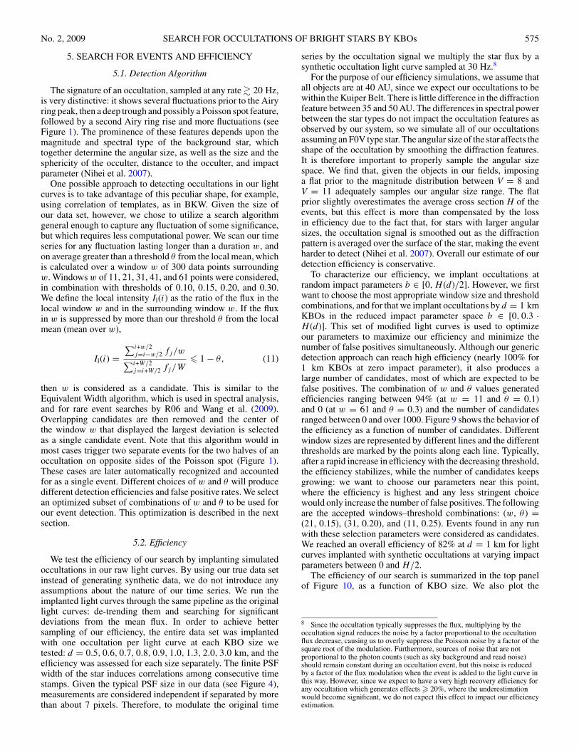
To characterize our efficiency, we implant occultations atrandom impact parameters b ∈ [0,H (d)/2]. However, we firstwant to choose the most appropriate window size and thresholdcombinations, and for that we implant occultations by d = 1 kmKBOs in the reduced impact parameter space b ∈ [0, 0.3 ·H (d)]. This set of modified light curves is used to optimizeour parameters to maximize our efficiency and minimize thenumber of false positives simultaneously. Although our genericdetection approach can reach high efficiency (nearly 100% for1 km KBOs at zero impact parameter), it also produces alarge number of candidates, most of which are expected to befalse positives. The combination of w and θ values generatedefficiencies ranging between 94% (at w = 11 and θ = 0.1)and 0 (at w = 61 and θ = 0.3) and the number of candidatesranged between 0 and over 1000. Figure 9 shows the behavior ofthe efficiency as a function of number of candidates. Differentwindow sizes are represented by different lines and the differentthresholds are marked by the points along each line. Typically,after a rapid increase in efficiency with the decreasing threshold,the efficiency stabilizes, while the number of candidates keepsgrowing: we want to choose our parameters near this point,where the efficiency is highest and any less stringent choicewould only increase the number of false positives. The followingare the accepted windows–threshold combinations: (w, θ ) =(21, 0.15), (31, 0.20), and (11, 0.25). Events found in any runwith these selection parameters were considered as candidates.We reached an overall efficiency of 82% at d = 1 km for lightcurves implanted with synthetic occultations at varying impactparameters between 0 and H/2.

The efficiency of our search is summarized in the top panelof Figure 10, as a function of KBO size. We also plot the

8 Since the occultation typically suppresses the flux, multiplying by theoccultation signal reduces the noise by a factor proportional to the occultationflux decrease, causing us to overly suppress the Poisson noise by a factor of thesquare root of the modulation. Furthermore, sources of noise that are notproportional to the photon counts (such as sky background and read noise)should remain constant during an occultation event, but this noise is reducedby a factor of the flux modulation when the event is added to the light curve inthis way. However, since we expect to have a very high recovery efficiency forany occultation which generates effects � 20%, where the underestimationwould become significant, we do not expect this effect to impact our efficiencyestimation.

576 BIANCO ET AL. Vol. 138

0

0.2

0.4

0.6

100 1000 10000candidates

effi

cien

cy

w=11w=21w=31w=41w=61

Figure 9. Efficiency plotted against the number of unidentified candidates(mostly false positives). Each line represents a different window size w, andeach point represents the value of the efficiency at threshold θ = 0.08, 0.10,0.15, 0.20, and 0.30, the number of false positives monotonically grows withdecreasing θ (larger values of θ on the left). All lines (all w values) show aplateau at different thresholds.

corresponding effective solid angle Ωe(d), defined as

Ωe(d) =∑

∗

H (d, θ∗)

D

vrel

DT∗ε(d, θ�), (12)

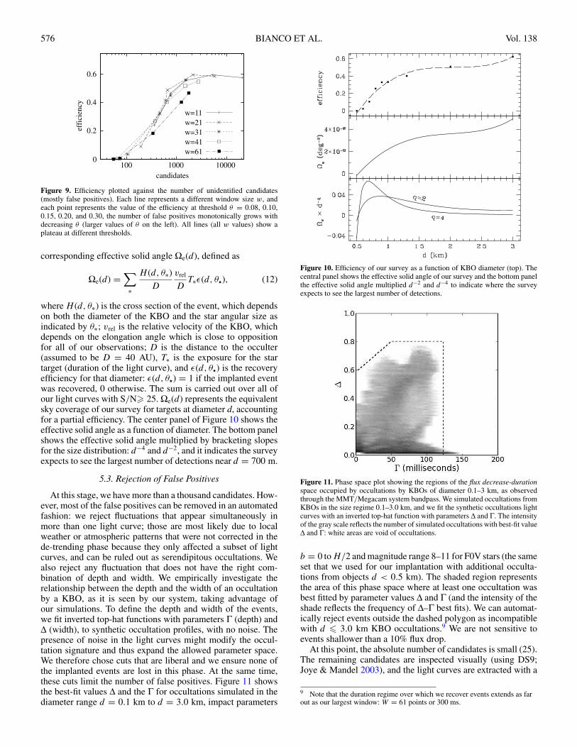
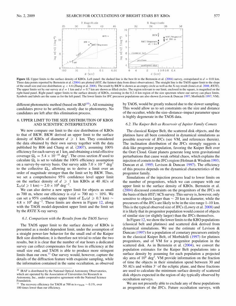
where H (d, θ∗) is the cross section of the event, which dependson both the diameter of the KBO and the star angular size asindicated by θ∗; vrel is the relative velocity of the KBO, whichdepends on the elongation angle which is close to oppositionfor all of our observations; D is the distance to the occulter(assumed to be D = 40 AU), T∗ is the exposure for the startarget (duration of the light curve), and ε(d, θ�) is the recoveryefficiency for that diameter: ε(d, θ�) = 1 if the implanted eventwas recovered, 0 otherwise. The sum is carried out over all ofour light curves with S/N� 25. Ωe(d) represents the equivalentsky coverage of our survey for targets at diameter d, accountingfor a partial efficiency. The center panel of Figure 10 shows theeffective solid angle as a function of diameter. The bottom panelshows the effective solid angle multiplied by bracketing slopesfor the size distribution: d−4 and d−2, and it indicates the surveyexpects to see the largest number of detections near d = 700 m.

5.3. Rejection of False Positives

At this stage, we have more than a thousand candidates. How-ever, most of the false positives can be removed in an automatedfashion: we reject fluctuations that appear simultaneously inmore than one light curve; those are most likely due to localweather or atmospheric patterns that were not corrected in thede-trending phase because they only affected a subset of lightcurves, and can be ruled out as serendipitous occultations. Wealso reject any fluctuation that does not have the right com-bination of depth and width. We empirically investigate therelationship between the depth and the width of an occultationby a KBO, as it is seen by our system, taking advantage ofour simulations. To define the depth and width of the events,we fit inverted top-hat functions with parameters Γ (depth) andΔ (width), to synthetic occultation profiles, with no noise. Thepresence of noise in the light curves might modify the occul-tation signature and thus expand the allowed parameter space.We therefore chose cuts that are liberal and we ensure none ofthe implanted events are lost in this phase. At the same time,these cuts limit the number of false positives. Figure 11 showsthe best-fit values Δ and the Γ for occultations simulated in thediameter range d = 0.1 km to d = 3.0 km, impact parameters

Figure 10. Efficiency of our survey as a function of KBO diameter (top). Thecentral panel shows the effective solid angle of our survey and the bottom panelthe effective solid angle multiplied d−2 and d−4 to indicate where the surveyexpects to see the largest number of detections.

Figure 11. Phase space plot showing the regions of the flux decrease-durationspace occupied by occultations by KBOs of diameter 0.1–3 km, as observedthrough the MMT/Megacam system bandpass. We simulated occultations fromKBOs in the size regime 0.1–3.0 km, and we fit the synthetic occultations lightcurves with an inverted top-hat function with parameters Δ and Γ. The intensityof the gray scale reflects the number of simulated occultations with best-fit valueΔ and Γ: white areas are void of occultations.

b = 0 to H/2 and magnitude range 8–11 for F0V stars (the sameset that we used for our implantation with additional occulta-tions from objects d < 0.5 km). The shaded region representsthe area of this phase space where at least one occultation wasbest fitted by parameter values Δ and Γ (and the intensity of theshade reflects the frequency of Δ–Γ best fits). We can automat-ically reject events outside the dashed polygon as incompatiblewith d � 3.0 km KBO occultations.9 We are not sensitive toevents shallower than a 10% flux drop.

At this point, the absolute number of candidates is small (25).The remaining candidates are inspected visually (using DS9;Joye & Mandel 2003), and the light curves are extracted with a

9 Note that the duration regime over which we recover events extends as farout as our largest window: W = 61 points or 300 ms.

No. 2, 2009 SEARCH FOR OCCULTATIONS OF BRIGHT STARS BY KBOs 577

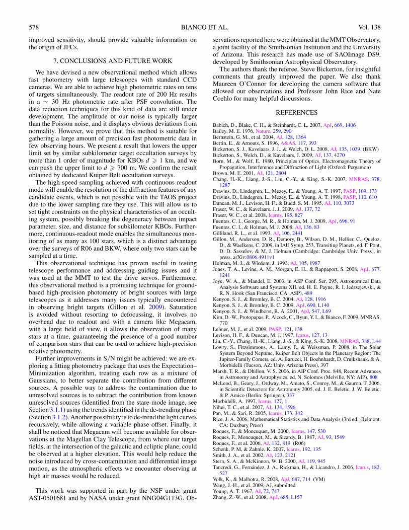
Figure 12. Upper limits to the surface density of KBOs. Left panel: the dashed line is the best fit to the Bernstein et al. (2004) survey, extrapolated to d = 0.01 km.Three data points reported by Bernstein et al. (2004) are plotted (HST, the faintest data from direct observations). The straight line is the TAOS upper limit to the slopeof the small size end size distribution: q < 4.6 (Zhang et al. 2008). The result by BKW is shown as an empty circle as well as the X-ray result (Jones et al. 2008; RXTE).The upper limits set by our survey at d = 1 km and d = 0.7 km are shown as filled circles. The region relevant to our limit, enclosed in the square, is magnified on theright-hand panel. Right panel: upper limits to the surface density of KBOs, zooming in the 0.2–6 km region of the size spectrum where our survey can place limits.Symbols and labels are the same as for the left panel. The lower limits for JFC precursor populations are also shown (Levison & Duncan 1997; Morbidelli 1997; VM).

different photometric method (based on IRAF10). All remainingcandidates prove to be artifacts, mostly due to photometry. Nocandidates are left after this elimination process.

6. UPPER LIMIT TO THE SIZE DISTRIBUTION OF KBOSAND SCIENTIFIC INTERPRETATION

We now compare our limit to the size distribution of KBOsto that of BKW. BKW derived an upper limit to the surfacedensity of KBOs of diameter d � 1 km. They consideredthe data obtained by their own survey together with the datapublished by R06 and Chang et al. (2007), assuming 100%efficiency for each survey at 1 km, and obtaining a total effectivecoverage Ωe = 5.4 × 10−10 deg2. The cross section H used tocalculate Ωe is set to validate the 100% efficiency assumptionon a survey-by-survey basis. Our survey adds 7.0 × 10−9 deg2

to the collective Ωe, allowing us to derive a limit over anorder of magnitude stronger than the limit set by BKW. Thus,we set a comprehensive 95% confidence level upper limiton the surface density of d � 1 km KBOs at 40 AUs ofΣN (d � 1 km) ∼ 2.0 × 108 deg−2.

We can also derive a new upper limit for objects as smallas 700 m, where our efficiency is ε(d = 700 m) ∼ 10%. Wecan set a 95% confidence upper limit of ΣN (d � 0.7 km) ∼4.8 × 108 deg−2. These limits are shown in Figure 12, alongwith the TAOS model-dependent upper limit and the limit setby the RXTE X-ray survey.

6.1. Comparison with the Results from the TAOS Survey

The TAOS upper limit to the surface density of KBOs ispresented as a model-dependent limit, under the assumption ofa straight power-law behavior for the small end of the KuiperBelt size distribution; it is therefore not trivial to relate the tworesults, but it is clear that the number of star hours a dedicatedsurvey can collect compensates for the loss in efficiency at thesmall size end, and TAOS is able to produce more stringentlimits than our own.11 Our survey would, however, capture thedetails of the diffraction feature with exquisite sampling, whilethe information contained in the same occultation, as observed

10 IRAF is distributed by the National Optical Astronomy Observatories,which are operated by the Association of Universities for Research inAstronomy, Inc., under cooperative agreement with the National ScienceFoundation.11 The recovery efficiency for TAOS at 700 m is εTAOS ∼ 0.1%, over100 times lower than our efficiency.

by TAOS, would be greatly reduced due to the slower sampling.This would allow us to set constraints on the size and distanceof the occulter, while the size–distance–impact parameter spaceis highly degenerate in the TAOS data.

6.2. The Kuiper Belt as Reservoir of Jupiter Family Comets

The classical Kuiper Belt, the scattered disk objects, and theplutinos have all been considered in dynamical simulations aspossible reservoir of JFCs (see VM, and references therein).The inclination distribution of the JFCs strongly suggests adisk-like progenitor population, favoring the Kuiper Belt overthe Oort Cloud. Giant planets generate long term gravitationalperturbations that cause weak orbital chaos, which explains theinjection of comets to the JFCs region (Holman & Wisdom 1993;Duncan et al. 1995; Levison & Duncan 1997). The efficiencyof this process depends on the dynamical characteristics of theprogenitor family.

Simulations of the injection process lead to lower limits onthe number of progenitors, which we can compare with ourupper limit to the surface density of KBOs. Bernstein et al.(2004) discussed constraints on the progenitors of the JFCs onthe basis of their HST/ACS survey. This survey is, however, onlysensitive to objects larger than ∼ 20 km in diameter, while theprecursors of the JFCs are likely to be in the size range 1–10 km.This is the typical observed size of JFCs (Lowry et al. 2008) andit is likely that its progenitor population would consist of objectsof similar size (or slightly larger) than the JFCs themselves.

In Figure 12, we show the lower limits to the KBO populations(classical belt and plutinos) and scattered disk derived fromdynamical simulations. We use the estimate of Levison &Duncan (1997) for a population of cometary precursors entirelyin the classical Kuiper Belt, of Morbidelli (1997) for plutinosprogenitors, and of VM for a progenitor population in thescattered disk. As in Bernstein et al. (2004), we convert thepopulation estimates for the Kuiper Belt populations into asurface density by assuming for each population a projectedsky area of 104 deg2. VM provide information on the fractionof time the objects in their simulation spend between 30 and50 AUs and within 3◦ of the ecliptic plane, and these fractionsare used to calculate the minimum surface density of scattereddisk objects expected in the region of sky typically observed byoccultation surveys.

We are not presently able to exclude any of these populationsas progenitors of the JFCs. Future occultation surveys, with

578 BIANCO ET AL. Vol. 138

improved sensitivity, should provide valuable information onthe origin of JFCs.

7. CONCLUSIONS AND FUTURE WORK

We have devised a new observational method which allowsfast photometry with large telescopes with standard CCDcameras. We are able to achieve high photometric rates on tensof targets simultaneously. The readout rate of 200 Hz resultsin a ∼ 30 Hz photometric rate after PSF convolution. Thedata reduction techniques for this kind of data are still underdevelopment. The amplitude of our noise is typically largerthan the Poisson noise, and it displays obvious deviations fromnormality. However, we prove that this method is suitable forgathering a large amount of precision fast photometric data infew observing hours. We present a result that lowers the upperlimit set by similar subkilometer target occultation surveys bymore than 1 order of magnitude for KBOs d � 1 km, and wecan push the upper limit to d � 700 m. We confirm the resultobtained by dedicated Kuiper Belt occultation surveys.

The high-speed sampling achieved with continuous-readoutmode will enable the resolution of the diffraction features of anycandidate events, which is not possible with the TAOS projectdue to the lower sampling rate they use. This will allow us toset tight constraints on the physical characteristics of an occult-ing system, possibly breaking the degeneracy between impactparameter, size, and distance for subkilometer KBOs. Further-more, continuous-readout mode enables the simultaneous mon-itoring of as many as 100 stars, which is a distinct advantageover the surveys of R06 and BKW, where only two stars can besampled at a time.

This observational technique has proven useful in testingtelescope performance and addressing guiding issues and itwas used at the MMT to test the drive servos. Furthermore,this observational method is a promising technique for ground-based high-precision photometry of bright sources with largetelescopes as it addresses many issues typically encounteredin observing bright targets (Gillon et al. 2009). Saturationis avoided without resorting to defocussing, it involves nooverhead due to readout and with a camera like Megacam,with a large field of view, it allows the observation of manystars at a time, guaranteeing the presence of a good numberof comparison stars that can be used to achieve high-precisionrelative photometry.

Further improvements in S/N might be achieved: we are ex-ploring a fitting photometry package that uses the Expectation–Minimization algorithm, treating each row as a mixture ofGaussians, to better separate the contribution from differentsources. A possible way to address the contamination due tounresolved sources is to subtract the contribution from knownunresolved sources (identified from the stare-mode image, seeSection 3.1.1) using the trends identified in the de-trending phase(Section 3.1.2). Another possibility is to de-trend the light curvesrecursively, while allowing a variable phase offset. Finally, itshall be noticed that Megacam will become available for obser-vations at the Magellan Clay Telescope, from where our targetfields, at the intersection of the galactic and ecliptic plane, couldbe observed at a higher elevation. This would help reduce thenoise introduced by cross-contamination and differential imagemotion, as the atmospheric effects we encounter observing athigh air masses would be reduced.

This work was supported in part by the NSF under grantAST-0501681 and by NASA under grant NNG04G113G. Ob-

servations reported here were obtained at the MMT Observatory,a joint facility of the Smithsonian Institution and the Universityof Arizona. This research has made use of SAOImage DS9,developed by Smithsonian Astrophysical Observatory.

The authors thank the referee, Steve Bickerton, for insightfulcomments that greatly improved the paper. We also thankMaureen O’Connor for developing the camera software thatallowed our observations and Professor John Rice and NateCoehlo for many helpful discussions.

REFERENCES

Babich, D., Blake, C. H., & Steinhardt, C. L. 2007, ApJ, 669, 1406Bailey, M. E. 1976, Nature, 259, 290Bernstein, G. M., et al. 2004, AJ, 128, 1364Bertin, E., & Arnouts, S. 1996, A&AS, 117, 393Bickerton, S. J., Kavelaars, J. J., & Welch, D. L. 2008, AJ, 135, 1039 (BKW)Bickerton, S., Welch, D., & Kavelaars, J. 2009, AJ, 137, 4270Born, M., & Wolf, E. 1980, Principles of Optics. Electromagnetic Theory of

Propagation, Interference and Diffraction of Light (Oxford: Pergamon)Brown, M. E. 2001, AJ, 121, 2804Chang, H.-K., Liang, J.-S., Liu, C.-Y., & King, S.-K. 2007, MNRAS, 378,

1287Dravins, D., Lindegren, L., Mezey, E., & Young, A. T. 1997, PASP, 109, 173Dravins, D., Lindegren, L., Mezey, E., & Young, A. T. 1998, PASP, 110, 610Duncan, M. J., Levison, H. F., & Budd, S. M. 1995, AJ, 110, 3073Fraser, W. C., & Kavelaars, J. J. 2009, AJ, 137, 72Fraser, W. C., et al. 2008, Icarus, 195, 827Fuentes, C. I., George, M. R., & Holman, M. J. 2009, ApJ, 696, 91Fuentes, C. I., & Holman, M. J. 2008, AJ, 136, 83Gilliland, R. L., et al. 1993, AJ, 106, 2441Gillon, M., Anderson, D. R., Demory, B., Wilson, D. M., Hellier, C., Queloz,

D., & Waelkens, C. 2009, in IAU Symp. 253, Transiting Planets, ed. F. Pont,D. D. Sasselov, & M. J. Holman (Cambridge: Cambridge Univ. Press), inpress, arXiv:0806.4911v1

Holman, M. J., & Wisdom, J. 1993, AJ, 105, 1987Jones, T. A., Levine, A. M., Morgan, E. H., & Rappaport, S. 2008, ApJ, 677,

1241Joye, W. A., & Mandel, E. 2003, in ASP Conf. Ser. 295, Astronomical Data

Analysis Software and Systems XII, ed. H. E. Payne, R. I. Jedrzejewski, &R. N. Hook (San Francisco, CA: ASP), 489

Kenyon, S. J., & Bromley, B. C. 2004, AJ, 128, 1916Kenyon, S. J., & Bromley, B. C. 2009, ApJ, 690, L140Kenyon, S. J., & Windhorst, R. A. 2001, ApJ, 547, L69Kim, D.-W., Protopapas, P., Alcock, C., Byun, Y. I., & Bianco, F. 2009, MNRAS,

770Lehner, M. J., et al. 2009, PASP, 121, 138Levison, H. F., & Duncan, M. J. 1997, Icarus, 127, 13Liu, C.-Y., Chang, H.-K., Liang, J.-S., & King, S.-K. 2008, MNRAS, 388, L44Lowry, S., Fitzsimmons, A., Lamy, P., & Weissman, P. 2008, in The Solar

System Beyond Neptune, Kuiper Belt Objects in the Planetary Region: TheJupiter-Family Comets, ed. A. Barucci, H. Boehnhardt, D. Cruikshank, & A.Morbidelli (Tucson, AZ: Univ. Arizona Press), 397

Marsh, T. R., & Dhillon, V. S. 2006, in AIP Conf. Proc. 848, Recent Advancesin Astronomy and Astrophysics, ed. N. Solomos (Melville, NY: AIP), 808

McLeod, B., Geary, J., Ordway, M., Amato, S., Conroy, M., & Gauron, T. 2006,in Scientific Detectors for Astronomy 2005, ed. J. E. Beletic, J. W. Beletic,& P. Amico (Berlin: Springer), 337

Morbidelli, A. 1997, Icarus, 127, 1Nihei, T. C., et al. 2007, AJ, 134, 1596Pan, M., & Sari, R. 2005, Icarus, 173, 342Rice, J. A. 2006, Mathematical Statistics and Data Analysis (3rd ed., Belmont,

CA: Duxbury Press)Roques, F., & Moncuquet, M. 2000, Icarus, 147, 530Roques, F., Moncuquet, M., & Sicardy, B. 1987, AJ, 93, 1549Roques, F., et al. 2006, AJ, 132, 819 (R06)Schenk, P. M, & Zahnle, K. 2007, Icarus, 192, 135Smith, J. A., et al. 2002, AJ, 123, 2121Stern, S. A., & McKinnon, W. B. 2000, AJ, 119, 945Tancredi, G., Fernandez, J. A., Rickman, H., & Licandro, J. 2006, Icarus, 182,

527Volk, K., & Malhotra, R. 2008, ApJ, 687, 714 (VM)Wang, J.-H., et al. 2009, AJ, submittedYoung, A. T. 1967, AJ, 72, 747Zhang, Z.-W., et al. 2008, ApJ, 685, L157