A simple linear time algorithm for cograph recognition

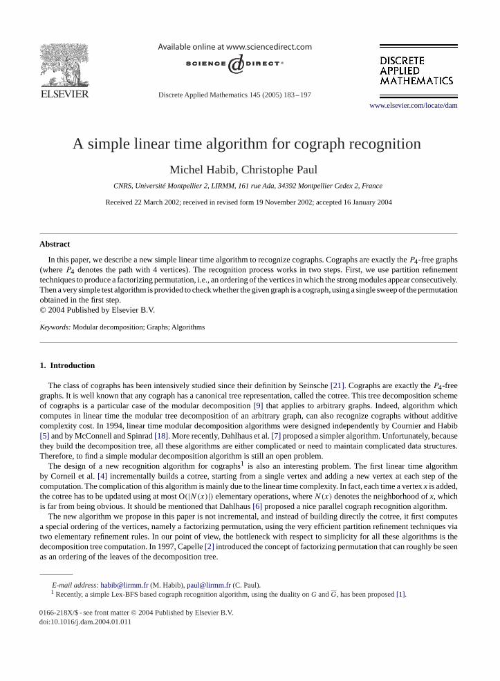
Discrete Applied Mathematics 145 (2005) 183–197

www.elsevier.com/locate/dam

A simple linear time algorithm for cograph recognition

Michel Habib, Christophe PaulCNRS, Université Montpellier 2, LIRMM, 161 rue Ada, 34392 Montpellier Cedex 2, France

Received 22 March 2002; received in revised form 19 November 2002; accepted 16 January 2004

Abstract

In this paper, we describe a new simple linear time algorithm to recognize cographs. Cographs are exactly theP4-free graphs(whereP4 denotes the path with 4 vertices). The recognition process works in two steps. First, we use partition refinementtechniques to produce a factorizing permutation, i.e., an ordering of the vertices in which the strong modules appear consecutively.Then a very simple test algorithm is provided to check whether the given graph is a cograph, using a single sweep of the permutationobtained in the first step.© 2004 Published by Elsevier B.V.

Keywords:Modular decomposition; Graphs; Algorithms

1. Introduction

The class of cographs has been intensively studied since their definition by Seinsche[21]. Cographs are exactly theP4-freegraphs. It is well known that any cograph has a canonical tree representation, called the cotree. This tree decomposition schemeof cographs is a particular case of the modular decomposition[9] that applies to arbitrary graphs. Indeed, algorithm whichcomputes in linear time the modular tree decomposition of an arbitrary graph, can also recognize cographs without additivecomplexity cost. In 1994, linear time modular decomposition algorithms were designed independently by Cournier and Habib[5] and by McConnell and Spinrad[18]. More recently, Dahlhaus et al.[7] proposed a simpler algorithm. Unfortunately, becausethey build the decomposition tree, all these algorithms are either complicated or need to maintain complicated data structures.Therefore, to find a simple modular decomposition algorithm is still an open problem.

The design of a new recognition algorithm for cographs1 is also an interesting problem. The first linear time algorithmby Corneil et al.[4] incrementally builds a cotree, starting from a single vertex and adding a new vertex at each step of thecomputation. The complication of this algorithm is mainly due to the linear time complexity. In fact, each time a vertexx is added,the cotree has to be updated using at most O(|N(x)|) elementary operations, whereN(x) denotes the neighborhood ofx, whichis far from being obvious. It should be mentioned that Dahlhaus[6] proposed a nice parallel cograph recognition algorithm.

The new algorithm we propose in this paper is not incremental, and instead of building directly the cotree, it first computesa special ordering of the vertices, namely a factorizing permutation, using the very efficient partition refinement techniques viatwo elementary refinement rules. In our point of view, the bottleneck with respect to simplicity for all these algorithms is thedecomposition tree computation. In 1997, Capelle[2] introduced the concept of factorizing permutation that can roughly be seenas an ordering of the leaves of the decomposition tree.

E-mail address:[email protected](M. Habib),[email protected](C. Paul).1 Recently, a simple Lex-BFS based cograph recognition algorithm, using the duality onG andG, has been proposed[1].

0166-218X/$ - see front matter © 2004 Published by Elsevier B.V.doi:10.1016/j.dam.2004.01.011

http://www.elsevier.com/locate/dam

mailto:[email protected]

mailto:[email protected]

184 M. Habib, C. Paul / Discrete Applied Mathematics 145 (2005) 183–197

Our algorithm really avoids complicated data structures because it never computes the decomposition tree. It is a two stepalgorithm. The first step only computes a permutation of the vertices, that is a factorizing permutation if the input graph is acograph. The second step tests the result: the computed permutation has a certain property iff the input graph is a cograph. Itroughly consists of a left to right scan of the computed permutation. Both steps of the algorithm need linear time and the mainstep is based on the powerful paradigm of partition refinement and vertex splitting; thus this algorithm can be included in a widepool of graphs algorithms including modular decomposition, transitive orientation, interval graph recognition algorithms. Theinterested reader can refer to[10,11] for more examples. In[8,11] a O(n + m logn) version of the first step was proposed. Ouralgorithm can also be seen as the first step towards a simple linear modular decomposition algorithm.

Section 2 presents in more detail the structure of cographs and some definitions. The algorithm that computes a factorizingpermutation of a cograph is explained in Section 3. Data-structures and complexity analysis are discussed in Section 4. Finally,the recognition test is detailed in Section 5.

2. Definitions

2.1. Cographs and factorizing permutations

Throughout this paper we consider only finite undirected simple (with no multiple edges) graphs.

Definition 1. The class of cographs is the smallest class of graphs containing the single vertex graph and closed under seriesand parallel composition.

Let G1 = (V1, E1) andG2 = (V2, E2) be two arbitrary graphs. A graphG = (V , E) is theparallel compositionof G1 andG2if V =V1 ∪V2 andE =E1 ∪E2. A graphG is theseries compositionof G1 andG2 if V =V1 ∪V2 andE =E1 ∪E2 ∪{(x1, x2)

s.t.x1 ∈ E1 andx2 ∈ E2}.Therefore, to each cograph can be associated several composition formulas using series and parallel operations. Such a formula

can be written as a tree whose leaves are the vertices of the graph, and the internal nodes are labeledseriesor parallel dependingof their corresponding operation. Among those tree-decompositions, for each graph there exists a canonical one, the so-calledcotree[4] in which on every path, the labels series and parallel strictly alternate.Fig. 1shows an example of a cograph and itscotree.

Remark 2. In a cotree, the internal nodes of a path from a leaf to the root are alternatively labeled series and parallel.

Remark 3. In a cograph, two verticesx andy are adjacent iff their least common ancestor (denoted byLCA(x, y)) in the cotreeis a series node.

Definition 4. Let us denote by�T the usual partial order of the nodes ofT (i.e., n1�T n2 iff n1 is a descendant ofn2 in T.Equality holds whenn1 = n2.)

parallel parallel

series

series

f

e

dc

ba

d

cb

a

e

f

Fig. 1. A cograph and its cotree.

M. Habib, C. Paul / Discrete Applied Mathematics 145 (2005) 183–197 185

Notation 1. Let n be an internal node of the cotreeT of a given cographG. Let us denote byTn the subtree ofT rooted atn.

Let M be the set of vertices that are leaves of some subtreeTn for somen. It follows from the second remark that any pair ofvertices inM have the same neighborhood outsideM; such a set is called amoduleand plays an important role in the cographrecognition algorithm. More formally:

Definition 5. A set of verticesM of a graphG is amoduleiff for any zandt in M, N(z)\M = N(t)\M. A moduleM is astrongmoduleiff for any moduleM ′ eitherM ′ ⊆ M or M ⊆ M ′ or M ∩ M ′ = ∅.

Remark 6. For any strong moduleM, there is an internal noden of the cotreeT such thatM is exactly the set of leaves ofTn.

The algorithm we present computes afactorizing permutation, that can be seen as a postorder traversal of the leaves of thecotree. Let us define this permutation more precisely.

Definition 7. A factorizing permutationof a graphG = (V , E) is a permutation� of the vertex setV such that the vertices ofany strong module ofG appears consecutively in�.

In particular if G is a prime graph (i.e., has no nontrivial module) then any permutation of the vertices is a factorizingpermutation. Let us now examine the relationships between cotrees and factorizing permutations. Although a given cographG has a unique cotreeT (G), a cotree admits several plane representations (drawings) in which root is on top and where theleft-right ordering of the children of each node is fixed. We first need a definition.

Definition 8. Let x, y, z be three different vertices. Thenx separates yandz if eitherxy ∈ E andxz /∈ E or xy /∈ E andxz ∈ E.

Lemma 9. Factorizing permutations are in one-to-one correspondence with plane representations of a cotree.

Proof. Let A be plane representation of a cotree, the left-right ordering of the leaves yields a factorizing permutation. Let usprove the converse by induction on the size ofG. If G has only one vertex the result is obvious. Now let� be a factorizingpermutation ofG. If G is prime its cotreeT (G) has only one internal node and the result is also obvious. ElseG admits a minimalnon trivial strong moduleM. By definitionM defines a factor of�. The result is obtained by contractingM to a single vertex andapplying induction. �

Most of the proofs of this paper can easily been understood geometrically when considering the plane representation associatedwith a given factorizing permutation. Furthermore, for cographs since adjacency between two vertices is completely determinedby their least common ancestor in the cotree, we can deduce some necessary conditions.

Corollary 10. Letx, y, z be distinct vertices appearing in that order in a factorizing permutation�. If x separates y and z thenLCA(x, y)<T LCA(y, z).

Proof. Let us considerA(�) the plane representation associated with�, thenz is a leaf ofA(�) that lies right toy which liesright to x. Trivially least common ancestors are the same in the cotree and inA(�). Let us consider the unique path inA(�)

joining y to the rootr of A(�). LCA(x, y) andLCA(y, z) are two nodes of this path. IfLCA(x, y)�T LCA(y, z) this implies thatLCA(x, y) = LCA(x, z) which contradicts the fact thatx separatesy andz. �

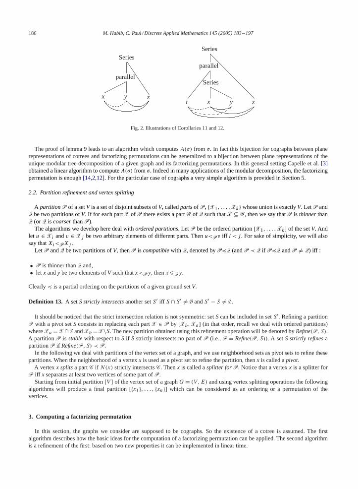
Corollary 11. Let x, y, z be distinct vertices appearing in that order in a factorizing permutation� such thatxy /∈ E andyz ∈ E. Thenxz ∈ E iff LCA(x, y)<T LCA(y, z) (seeFig. 2).

Proof. If xz ∈ E, thenx separatesy andz and Corollary 10 applies. Ifxz /∈ E, thenz separatesx andy. Same proof than forCorollary 10 shows thatLCA(x, y)>T LCA(y, z). �

Corollary 12. Let t, x, y, z be distinct vertices appearing in that order in a factorizing permutation� andtx /∈ E, xy ∈ E andxz ∈ E. If t separates y and z, then necessarilyty /∈ E andtz ∈ E (seeFig. 2).

Proof. Suppose the contrary:ty ∈ E and tz /∈ E. Corollary 11 applied to triplest, x, y and t, x, z, respectively, shows thatLCA(x, t)<T LCA(x, y) andLCA(x, z)<T LCA(x, t). It follows thatLCA(x, z)<T LCA(x, y) which would lead to a crossing inA(�), a contradiction. �


Series

xt y zx y z

parallel

Series

Series

parallel

Fig. 2. Illustrations of Corollaries 11 and 12.

The proof of lemma 9 leads to an algorithm which computesA(�) from �. In fact this bijection for cographs between planerepresentations of cotrees and factorizing permutations can be generalized to a bijection between plane representations of theunique modular tree decomposition of a given graph and its factorizing permutations. In this general setting Capelle et al.[3]obtained a linear algorithm to computeA(�) from �. Indeed in many applications of the modular decomposition, the factorizingpermutation is enough[14,2,12]. For the particular case of cographs a very simple algorithm is provided in Section 5.

2.2. Partition refinement and vertex splitting

A partitionP of a setV is a set of disjoint subsets ofV, calledpartsof P, {X1, . . . ,Xk} whose union is exactlyV. LetP andQ be two partitions ofV. If for each partX of P there exists a partY of Q such thatX ⊆ Y, then we say thatP is thinnerthanQ (orQ is coarserthanP).

The algorithms we develop here deal withordered partitions. LetP be the ordered partition[X1, . . . ,Xk] of the setV. Andlet u ∈ Xi andv ∈ Xj be two arbitrary elements of different parts. Thenu<Pv iff i < j . For sake of simplicity, we will alsosay thatXi<PXj .

LetP andQ be two partitions ofV, thenP is compatiblewith Q, denoted byP�Q (andP ≺ Q if P�Q andP �= Q) iff :

• P is thinner thanQ and,• let x andy be two elements ofV such thatx<Py, thenx �Qy.

Clearly� is a partial ordering on the partitions of a given ground setV.

Definition 13. A setS strictly intersectsanother setS′ iff S ∩ S′ �= ∅ andS′ − S �= ∅.

It should be noticed that the strict intersection relation is not symmetric: setScan be included in setS′. Refining a partitionP with a pivot setSconsists in replacing each partX ∈ P by [Xb,Xa] (in that order, recall we deal with ordered partitions)whereXa =X∩ S andXb =X\S. The new partition obtained using this refinement operation will be denoted byRefine(P, S).A partitionP is stablewith respect toS if Sstrictly intersects no part ofP (i.e.,P = Refine(P, S)). A setS strictly refinesapartitionP if Refine(P, S) ≺ P.

In the following we deal with partitions of the vertex set of a graph, and we use neighborhood sets as pivot sets to refine thesepartitions. When the neighborhood of a vertexx is used as a pivot set to refine the partition, thenx is called apivot.

A vertexx splitsa partC if N(x) strictly intersectsC. Thenx is called asplitter forP. Notice that a vertexx is a splitter forP iff x separates at least two vertices of some part ofP.

Starting from initial partition[V ] of the vertex set of a graphG = (V , E) and using vertex splitting operations the followingalgorithms will produce a final partition[{x1}, . . . , {xn}] which can be considered as an ordering or a permutation of thevertices.

3. Computing a factorizing permutation

In this section, the graphs we consider are supposed to be cographs. So the existence of a cotree is assumed. The firstalgorithm describes how the basic ideas for the computation of a factorizing permutation can be applied. The second algorithmis a refinement of the first: based on two new properties it can be implemented in linear time.


n2 nk. . .n1

x. . .

y

series

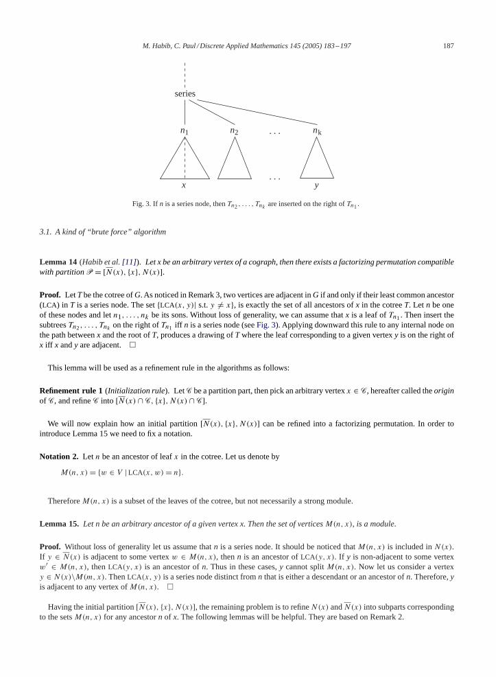
Fig. 3. If n is a series node, thenTn2, . . . , Tnkare inserted on the right ofTn1.

3.1. A kind of “brute force” algorithm

Lemma 14 (Habib et al.[11] ). Let x be an arbitrary vertex of a cograph, then there exists a factorizing permutation compatiblewith partitionP = [N(x), {x}, N(x)].

Proof. LetT be the cotree ofG. As noticed in Remark 3, two vertices are adjacent inG if and only if their least common ancestor(LCA) in T is a series node. The set{LCA(x, y)| s.t.y �= x}, is exactly the set of all ancestors ofx in the cotreeT. Let n be oneof these nodes and letn1, . . . , nk be its sons. Without loss of generality, we can assume thatx is a leaf ofTn1. Then insert thesubtreesTn2, . . . , Tnk on the right ofTn1 iff n is a series node (seeFig. 3). Applying downward this rule to any internal node onthe path betweenx and the root ofT, produces a drawing ofT where the leaf corresponding to a given vertexy is on the right ofx iff x andy are adjacent. �

This lemma will be used as a refinement rule in the algorithms as follows:

Refinement rule 1(Initialization rule). LetC be a partition part, then pick an arbitrary vertexx ∈ C, hereafter called theoriginof C, and refineC into [N(x) ∩ C, {x}, N(x) ∩ C].

We will now explain how an initial partition[N(x), {x}, N(x)] can be refined into a factorizing permutation. In order tointroduce Lemma 15 we need to fix a notation.

Notation 2. Let n be an ancestor of leafx in the cotree. Let us denote by

M(n, x) = {w ∈ V | LCA(x, w) = n}.

ThereforeM(n, x) is a subset of the leaves of the cotree, but not necessarily a strong module.

Lemma 15. Let n be an arbitrary ancestor of a given vertex x. Then the set of verticesM(n, x), is a module.

Proof. Without loss of generality let us assume thatn is a series node. It should be noticed thatM(n, x) is included inN(x).If y ∈ N(x) is adjacent to some vertexw ∈ M(n, x), thenn is an ancestor ofLCA(y, x). If y is non-adjacent to some vertexw′ ∈ M(n, x), thenLCA(y, x) is an ancestor ofn. Thus in these cases,y cannot splitM(n, x). Now let us consider a vertexy ∈ N(x)\M(m, x). ThenLCA(x, y) is a series node distinct fromn that is either a descendant or an ancestor ofn. Therefore,yis adjacent to any vertex ofM(n, x). �

Having the initial partition[N(x), {x}, N(x)], the remaining problem is to refineN(x) andN(x) into subparts correspondingto the setsM(n, x) for any ancestorn of x. The following lemmas will be helpful. They are based on Remark 2.


N (x)

N (x) N (z)

x

parallel

series

parallel

series

yz

N (x) N (z)

N (x)

⊃

⊃

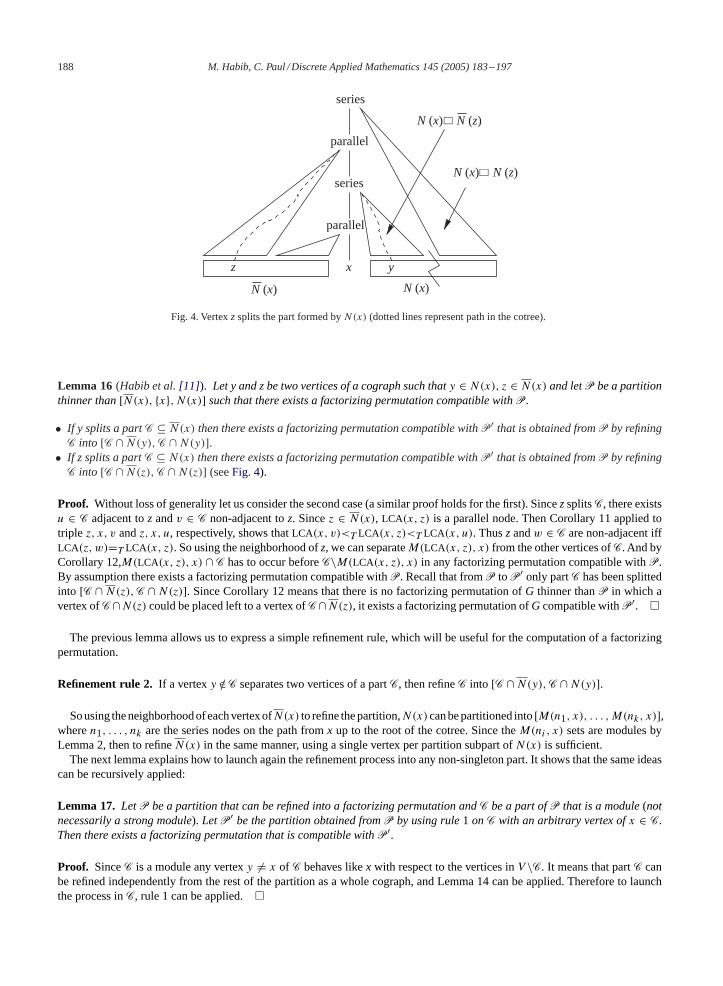
Fig. 4. Vertexz splits the part formed byN(x) (dotted lines represent path in the cotree).

Lemma 16 (Habib et al.[11] ). Let y and z be two vertices of a cograph such thaty ∈ N(x), z ∈ N(x) and letP be a partitionthinner than[N(x), {x}, N(x)] such that there exists a factorizing permutation compatible withP.

• If y splits a partC ⊆ N(x) then there exists a factorizing permutation compatible withP′ that is obtained fromP by refiningC into [C ∩ N(y),C ∩ N(y)].

• If z splits a partC ⊆ N(x) then there exists a factorizing permutation compatible withP′ that is obtained fromP by refiningC into [C ∩ N(z),C ∩ N(z)] (seeFig. 4).

Proof. Without loss of generality let us consider the second case (a similar proof holds for the first). SincezsplitsC, there existsu ∈ C adjacent toz andv ∈ C non-adjacent toz. Sincez ∈ N(x), LCA(x, z) is a parallel node. Then Corollary 11 applied totriple z, x, v andz, x, u, respectively, shows thatLCA(x, v)<T LCA(x, z)<T LCA(x, u). Thusz andw ∈ C are non-adjacent iffLCA(z, w)=T LCA(x, z). So using the neighborhood ofz, we can separateM(LCA(x, z), x) from the other vertices ofC. And byCorollary 12,M(LCA(x, z), x) ∩ C has to occur beforeC\M(LCA(x, z), x) in any factorizing permutation compatible withP.By assumption there exists a factorizing permutation compatible withP. Recall that fromP toP′ only partC has been splittedinto [C ∩ N(z),C ∩ N(z)]. Since Corollary 12 means that there is no factorizing permutation ofG thinner thanP in which avertex ofC∩N(z) could be placed left to a vertex ofC∩N(z), it exists a factorizing permutation ofG compatible withP′. �

The previous lemma allows us to express a simple refinement rule, which will be useful for the computation of a factorizingpermutation.

Refinement rule 2. If a vertexy /∈C separates two vertices of a partC, then refineC into [C ∩ N(y),C ∩ N(y)].

So using the neighborhood of each vertex ofN(x) to refine the partition,N(x) can be partitioned into[M(n1, x), . . . , M(nk, x)],wheren1, . . . , nk are the series nodes on the path fromx up to the root of the cotree. Since theM(ni, x) sets are modules byLemma 2, then to refineN(x) in the same manner, using a single vertex per partition subpart ofN(x) is sufficient.

The next lemma explains how to launch again the refinement process into any non-singleton part. It shows that the same ideascan be recursively applied:

Lemma 17. LetP be a partition that can be refined into a factorizing permutation andC be a part ofP that is a module(notnecessarily a strong module). LetP′ be the partition obtained fromP by using rule1 onC with an arbitrary vertex ofx ∈ C.Then there exists a factorizing permutation that is compatible withP′.

Proof. SinceC is a module any vertexy �= x of C behaves likex with respect to the vertices inV \C. It means that partC canbe refined independently from the rest of the partition as a whole cograph, and Lemma 14 can be applied. Therefore to launchthe process inC, rule 1 can be applied.�


Invariant of algorithm 1. There exists a factorizing permutation compatible with the current ordered partitionP.

Proof. Initially true, this invariant is proved for step 1 using Lemma 14, and for step 2 using Lemma 16. After step 2, any partC ⊆ N(x) corresponds to a setM(n, x) for some ancestorn of x. So by Lemma 15, it is a module. Therefore during step 3, therefining rule (2) can be applied just to one vertex per subpart ofN(x). By Lemma 16 the invariant is preserved.

Applying the same argument, we prove that after steps 2 and 3, necessarily all non-singleton parts ofP are modules of G.Since we only refine the partition when needed, a part which cannot be separated is necessarily maximal with this property andtherefore by Lemma 17 step 1 can be recursively processed.�

The correctness of Algorithm 1 follows from the above invariant that states:

Theorem 18. If G is a cograph, then Algorithm1 ends up with a final partitionP which is a factorizing permutation of G.

3.2. A linear time algorithm

Clearly the complexity of the above algorithm 1 is not linear since a given vertex can be used O(n) times as a pivot to refinethe partition: it implies a time-complexity larger than O(nm) or O(mlogn) if the partC is chosen via a cleverer rule[19].

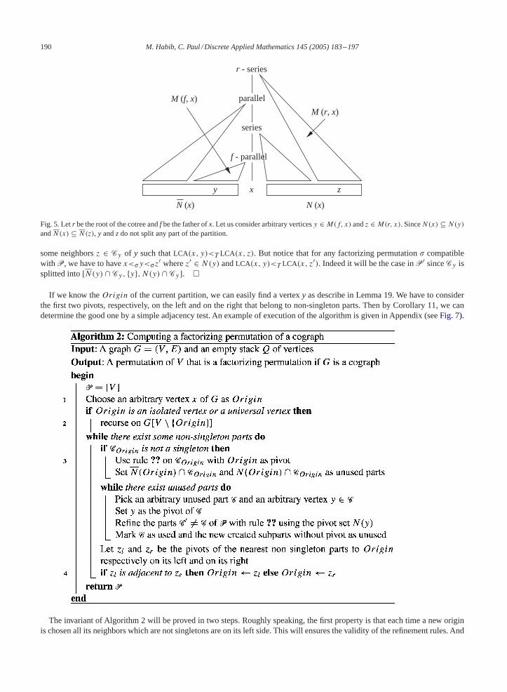
To achieve linear time complexity we need to use only O(1) time the neighborhood of each vertex. The problem is now tochoose the pivot vertices in an appropriate ordering. Indeed, as shown inFig. 5, an arbitrary choice may give a vertex whoseneighborhood does not refine the partition.

The idea of the algorithm is to use only one vertex per part as long as possible. When any part has a pivot that has been used,we have to find a way to relaunch the refinement process. The next lemma explain how it can be achieved using rule 1 can beused again. In the following, we will denote byCy the part containing a given vertexy.

Lemma 19. Let G = (V , E) be a cograph andP be a partition with vertex x asOrigin, that can be refined into a fac-torizing permutation. Lety ∈ Cy be a pivot. Let us assume that any vertex z such thatLCA(x, z) is a descendant ofLCA(x, y)(LCA(x, z)<T LCA(x, y)) belongs to a singleton part. LetP′ be the partition obtained fromP by splittingCy into[N(y) ∩ Cy, {y}, N(y) ∩ Cy ]. Then there exists a factorizing permutation compatible withP′.

Proof. Without loss of generality, let us assume thaty ∈ N(x).Any vertexv ∈ N(x) such thatv /∈ M(LCA(x, y), x) is a neighborof y. IndeedLCA(y, v) is a series node that is either a descendant or an ancestor ofLCA(x, y). If LCA(x, v)<T LCA(x, y), byassumptionv belongs to a singleton part and thus does not belong toCy . If LCA(y, v)>T LCA(x, y), thenv may belong toCy ornot. The simple case holds whenCy = M(LCA(x, y), x) and is proved by Lemma 17. But by assumption there may also exist


N (x) N (x)

y x

f - parallel

series

parallel

r - series

M (r, x)

M (f, x)

z

Fig. 5. Letr be the root of the cotree andf be the father ofx. Let us consider arbitrary verticesy ∈ M(f, x) andz ∈ M(r, x). SinceN(x) ⊆ N(y)

andN(x) ⊆ N(z), y andz do not split any part of the partition.

some neighborsz ∈ Cy of y such thatLCA(x, y)<T LCA(x, z). But notice that for any factorizing permutation� compatiblewith P, we have to havex<�y<�z′ wherez′ ∈ N(y) andLCA(x, y)<T LCA(x, z′). Indeed it will be the case inP′ sinceCy issplitted into[N(y) ∩ Cy, {y}, N(y) ∩ Cy ]. �

If we know theOrigin of the current partition, we can easily find a vertexy as describe in Lemma 19. We have to considerthe first two pivots, respectively, on the left and on the right that belong to non-singleton parts. Then by Corollary 11, we candetermine the good one by a simple adjacency test. An example of execution of the algorithm is given in Appendix (seeFig. 7).

The invariant of Algorithm 2 will be proved in two steps. Roughly speaking, the first property is that each time a new originis chosen all its neighbors which are not singletons are on its left side. This will ensures the validity of the refinement rules. And


thus at any step, there is a factorizing permutation compatible with the current partition. Let us introduce some notations:

• Let x0 be the first origin chosen at step 1 andxi be thei + 1th vertex chosen as the new origin of the partition (step 4).• The part containingxi and the partition at the step in whichxi becomes the current origin are denoted, respectively, byCi

andPi .• The invariant deals with subsetsVi of the vertex setV and cotreesTi of the subgraphs induced byVi . We defineV0 = V and

Vi = Vi−1\Mi , i > 0, whereMi = M(ni, xi−1) with ni the son ofLCA(xi , xi−1) in the cotreeTi . Let us remark that byLemma 15,Mi is a module for the subgraph induced byVi−1.

Invariant of algorithm 2. LetP be the current partition with originxi . If G is a cograph, then:

a: Let y be a vertex ofVi . Thenyxi ∈ E iff xi<Py.b: there exists a factorizing permutation compatibleP.

Proof.

• Invariant a. The property is clearly true in the casei = 0, since the initial partitionP0 is [N(x0), {x0}, N(x0)] (see step1). Let us assume by induction that invariantA holds for i �0. Let us consider a vertexy ∈ Vi+1. Let us remark thatLCA(y, xi)�Ti

LCA(xi+1, xi). Therefore,LCA(y, xi)=LCA(y, xi+1). Sinceyxi ∈ E iff y>Pixi , we also haveyxi+1 ∈ E

iff y>P1xi+1.

• Invariant b. In the following, all the partition we deal with, are issued from the refinement process.Invariant B is initiallytrue by Lemma 14 forP0. Let us consider any partitionP that is coarser thanP1. P is obtained by successive applicationof rule 2 and thus Lemma 16 ensures that the invariant is preserved. Let us assume by induction invariantB for anyP strictlycoarser thanPi with i �1. Let us first considerPi . By Corollary 11, the the new originxi checks (see step 4) the hypothesisof Lemma 19. Thus the refinement process can be relaunched onCi using rule 1. Soinvariant B is verified forPi . Nowrecall that by the choice ofxi , Mi is composed by singleton parts. It means that the problem of computing a factorizingpermutation on the subgraph induced byMi is solved. SinceMi is a module (that containsxi−1) for the subgraph inducedby Vi−1, Pi is stable with respect to the neighborhood of any vertex ofMi . In other words,Mi can be removed to end therefinement process. LetP′

ibe the partition ofVi obtained fromPi by removing the vertices of all theMj , j � i. Now there

exists a factorizing permutation of the induced subgraphG[V \Mi ] compatible withP′i. Since byinvariant A, P′

iis thinner

than[N(xi), {xi}, N(xi)], exactly the same arguments than those used for the initial case while there are some unused parts,shows that the property also holds for the current partitionP at any step of the refinement process.�

The above invariant proves the following theorem that states the correctness of Algorithm 2:

Theorem 20. Algorithm2 computes a factorizing permutation if the input graph is a cograph.

Proof. When any part is a singleton part, sinceinvariant B has been preserved by any refinement step, the partitionP is afactorizing permutation. �

4. Data-structures and complexity issues

In this section, we describe the data-structures and the key points of algorithm 2. The complexity of these operations will beproved. Then the complexity analysis of the whole algorithm follows.

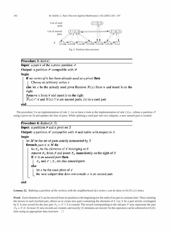
A partitionP of a setE is represented as shown inFig. 6. The elements ofE are stored in a sorted list and each element has apointer to its part. Since the elements of a given part are consecutive in the sorted list, each part can be represented with pointersto its first and last elements. The parts of the partition are stored in two different sorted lists depending on their status: one list oftheusedparts and one list for theunusedparts. To each used part, we have to store its vertex that has been used as a pivot. Thatvertex will be used once more at step 3 of algorithm 2.

Lemma 21. The neighborhood of each vertex is used at most once by procedure3, that can be processed inO(|N(x)|) times.

Proof. A vertex in a used partC can be used once more by procedure 3 iffC is split into subparts. Since the vertexx used inprocedure 3 is the only member of a new used part, it will never be used again. Procedure 3 can clearly be achieved in O(|N(x)|)time since we mainly have to move the neighbors ofx in the list of vertices. �


List of unusedparts

List of usedparts

E x5 x7x6

= [1, 4] = [6, 7]

= [5, 5]

x2 x3 x4x1

Fig. 6. Partition data-structure.

The procedure 3 is an implementation of rule 1. Let us have a look at the implementation of rule 2 (i.e., refines a partitionP

using a pivot setS) and updates the lists of parts. While splitting a used part into two subparts, a new unused part is created.

Lemma 22. Refining a partition of the vertices with the neighborhood of a vertex x can be done inO(|N(x)|) times.

Proof. Each element ofScan be moved from its position to the beginning (or the end) of its part in constant time. Then countingthe moves in each touched part, allows us to create new parts containing the elements ofS. LetX be a part strictly overlappedby S. A new record for the new partXa = X ∩ S is created. The record corresponding to the old partX now represents the partXb =X\S. At most|S| new records are created, and exactly|S| elements are moved. So this operation can be achieved in O(|S|)time using an appropriate data structure.�


In order to implement efficiently step 4 of algorithm 2, each time a vertex of a singleton partC is used as pivot with rule 2,the partC is removed from the lists of parts. Also when the origin of the partition changes, the part containing the part of the oldorigin is removed from the lists of parts. Therefore, to choose the new origin, we just have to look at the pivots of the two partsadjacent to the part containing the origin.

Lemma 23. The neighborhood of each vertex is used at most3 times to refine the partition.

Proof. The neighborhood of a given vertexx can be used to refine the partition with rule 2. It can also be used for the adjacencytest at step 4 of algorithm 2. To test whether the two candidates are connected or not, it suffices to scan the smallest neighborhoodand this search could be charged to the chosen new origin. Thus in the whole any neighborhood can be charged at most once atstep 4. The next use ofN(x) is to refine its partition part with rule 1 when it becomes the new origin, with procedure 3.�

Theorem 24. The algorithm2 computes a factorizing permutation of a cograph inO(n + m) time.

Proof. By Lemma 23, during the whole refining process each neighborhood is used O(1) times. So the whole complexity isO(

∑x∈V |N(x)|) = O(n + m). �

5. A very simple recognition test

Let us now consider the testing problem, i.e. to test whether the output permutation of algorithm 2 is a factorizing permutationor not. This work can easily be done in linear time using the following simple algorithm that scans the given permutation fromleft to right.

It is well known that any cograph admits a twin-elimination ordering of its vertex set defined as following :� = x1, . . . , xn

such that for any vertexxi , 1� i < n, there existsj, i < j �n such thatxi andxj are eithertrue twinsor false twins.

Definition 25. Two verticesx andy of a graphG are false (respectively true) twins iffN(x)=N(y) (resp.N(x)∪{x}=N(y)∪{y}).

Clearly two verticesx andy are twins iff they are brothers in the cotree (true twins if their parent nodeLCA(x, y) is a seriesnode, false otherwise). By definition, many brothers will occur consecutively in a factorizing permutation. The natural idea is to


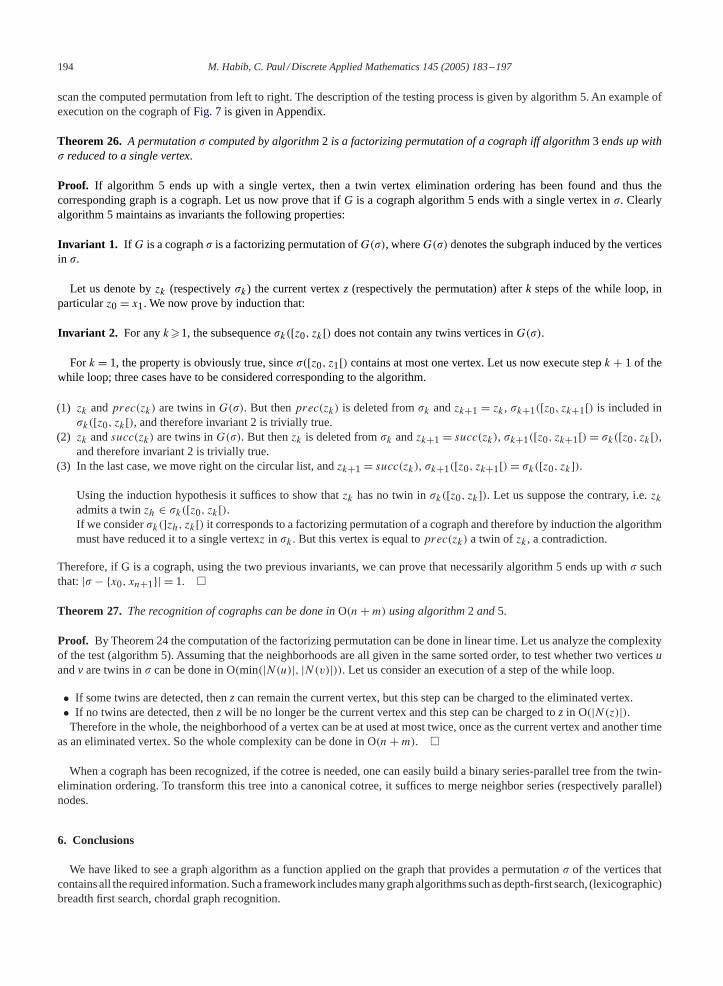
scan the computed permutation from left to right. The description of the testing process is given by algorithm 5. An example ofexecution on the cograph ofFig. 7 is given in Appendix.

Theorem 26. A permutation� computed by algorithm2 is a factorizing permutation of a cograph iff algorithm3 ends up with� reduced to a single vertex.

Proof. If algorithm 5 ends up with a single vertex, then a twin vertex elimination ordering has been found and thus thecorresponding graph is a cograph. Let us now prove that ifG is a cograph algorithm 5 ends with a single vertex in�. Clearlyalgorithm 5 maintains as invariants the following properties:

Invariant 1. If G is a cograph� is a factorizing permutation ofG(�), whereG(�) denotes the subgraph induced by the verticesin �.

Let us denote byzk (respectively�k) the current vertexz (respectively the permutation) afterk steps of the while loop, inparticularz0 = x1. We now prove by induction that:

Invariant 2. For anyk�1, the subsequence�k([z0, zk[) does not contain any twins vertices inG(�).

For k = 1, the property is obviously true, since�([z0, z1[) contains at most one vertex. Let us now execute stepk + 1 of thewhile loop; three cases have to be considered corresponding to the algorithm.

(1) zk andprec(zk) are twins inG(�). But thenprec(zk) is deleted from�k andzk+1 = zk , �k+1([z0, zk+1[) is included in�k([z0, zk[), and therefore invariant 2 is trivially true.

(2) zk andsucc(zk) are twins inG(�). But thenzk is deleted from�k andzk+1 = succ(zk), �k+1([z0, zk+1[) = �k([z0, zk[),and therefore invariant 2 is trivially true.

(3) In the last case, we move right on the circular list, andzk+1 = succ(zk), �k+1([z0, zk+1[) = �k([z0, zk]).

Using the induction hypothesis it suffices to show thatzk has no twin in�k([z0, zk]). Let us suppose the contrary, i.e.zk

admits a twinzh ∈ �k([z0, zk[).If we consider�k(]zh, zk[) it corresponds to a factorizing permutation of a cograph and therefore by induction the algorithmmust have reduced it to a single vertexz in �k . But this vertex is equal toprec(zk) a twin of zk , a contradiction.

Therefore, if G is a cograph, using the two previous invariants, we can prove that necessarily algorithm 5 ends up with� suchthat:|� − {x0, xn+1}| = 1. �

Theorem 27. The recognition of cographs can be done inO(n + m) using algorithm2 and5.

Proof. By Theorem 24 the computation of the factorizing permutation can be done in linear time. Let us analyze the complexityof the test (algorithm 5). Assuming that the neighborhoods are all given in the same sorted order, to test whether two verticesuandv are twins in� can be done in O(min(|N(u)|, |N(v)|)). Let us consider an execution of a step of the while loop.

• If some twins are detected, thenz can remain the current vertex, but this step can be charged to the eliminated vertex.• If no twins are detected, thenz will be no longer be the current vertex and this step can be charged toz in O(|N(z)|).Therefore in the whole, the neighborhood of a vertex can be at used at most twice, once as the current vertex and another time

as an eliminated vertex. So the whole complexity can be done in O(n + m). �

When a cograph has been recognized, if the cotree is needed, one can easily build a binary series-parallel tree from the twin-elimination ordering. To transform this tree into a canonical cotree, it suffices to merge neighbor series (respectively parallel)nodes.

6. Conclusions

We have liked to see a graph algorithm as a function applied on the graph that provides a permutation� of the vertices thatcontains all the required information. Such a framework includes many graph algorithms such as depth-first search, (lexicographic)breadth first search, chordal graph recognition.


It may turn out that even if the input graph is not a cograph algorithm 2 may output a factorizing permutation. Just consider thecase of theP4 for which any permutation of its vertex set is a factorizing permutation. So to recognize cographs, the recognitiontest has to be performed after algorithm 2. For those reasons the presented algorithm can be considered as a robust algorithm[20]:

• If the test fails, then it produces a certificate, namely the subgraphG(�), that shows the input graph is not a cograph. To bea little more precise, ifTG is the modular decomposition tree ofG, thenTG(�) is the tree obtained fromTG by recursivelydeleting all series and parallel nodes whose children are only leaves. IfG is not a cograph, thenTG(�) contains a prime nodeand soG(�) contains aP4.

• But also since it is possible to extract in linear time the modular tree decomposition out of a factorizing permutation[2], thesame algorithm may be used to recognize more general graph classes: for example graphs having with fewP4 [13,15–17].

Of course, another natural generalization of these ideas would be to apply them to modular decomposition. It has still to bedone, since the algorithm developed in[11] has an extralogn factor.

Acknowledgements

The authors wish to thank the anonymous referees for their careful reading and their useful remarks which greatly help us toimprove and simplify the paper.

Appendix A. An example

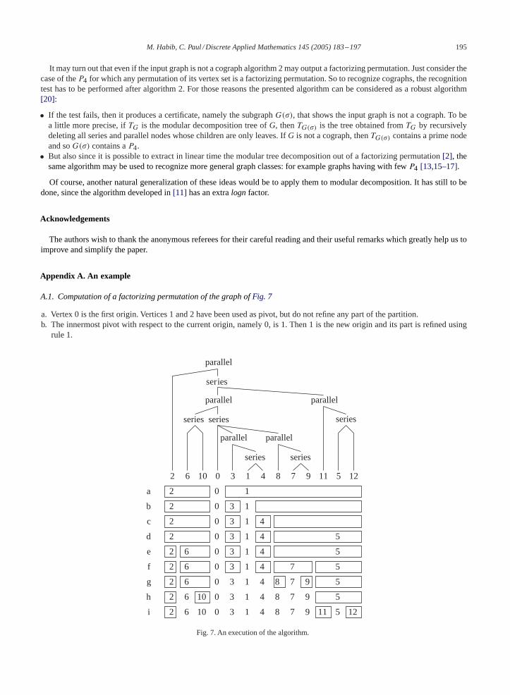
A.1. Computation of a factorizing permutation of the graph ofFig. 7

a. Vertex 0 is the first origin. Vertices 1 and 2 have been used as pivot, but do not refine any part of the partition.b. The innermost pivot with respect to the current origin, namely 0, is 1. Then 1 is the new origin and its part is refined using

rule 1.

parallel

parallel

parallel

parallel parallel

2 6 10 0 3 1 4 8 7 9 11 5 12

a

b

c

2

2

2

2 1

1

13

3

4

413

series series

seriesseries series

series

e

f

g

d

h

i 2

2

2

2

2 6

6

6

6 10 0

0

0

0

0

0

0

0

3

30106 1 4 8 9 11 5 12

5

5

5

5

5

7

7

7

7

9

98

8413

1 4

413

3 1 4

Fig. 7. An execution of the algorithm.


c. Vertex 3 splits the rightmost part into[4] and[8, 7, 9, 11, 5, 12]. Then vertex 4 can be used but it does not refine anything.d. Vertex 5 is used and splits the part containing 2 into[2] and[6, 10].e. Vertex 6 is used and splits the part containing 5 into[8, 7, 9] and[11, 5, 12].f. Vertex 7 is used but refines nothing.g. All the parts have been used. The innermost pivot with respect to the current origin, namely 1, is 7. The part containing 7 is

refined using rule 1 into[8], [7] and[9]. Vertices 8 and 9 can be used but refines nothing.h. All the parts have been used. The innermost pivot with respect to the current origin, namely 7, is 6. The part containing 6 is

refined using rule 1 into[6] and[10]. Vertex 10 can be used but refines nothing.i. All the parts have been used. The innermost pivot with respect to the current origin, namely 6, is 5. The part containing 5 is

refined using rule 1 into[11][5] and[10]. Now all parts are singletons, we are done.

A.2. The recognition test

• � = [x0, 2, 6, 10, 0, 3, 1, 4, 8, 7, 9, 11, 5, 12, x14]· z = 2: 2 andx0 nor 2 and 6 are twins.· z = 6: 6 and 2 are not twins but 6 and 10 are. Thus setz = 10 and 6 is removed.

• � = [x0, 2, 10, 0, 3, 1, 4, 8, 7, 9, 11, 5, 12, x14]· z = 10: 10 and 2 nor 10 and 0 are twins.· z = 0: 0 and 10 nor 0 and 3 are twins.· z = 3: 3 and 0 nor 3 and 1 are twins.· z = 1: 1 and 3 are not twins but 1 and 4 are. Thus setz = 4 and 1 is removed.

• � = [x0, 2, 10, 0, 3, 4, 8, 7, 9, 11, 5, 12, x14], z = 4: 4 and 3 are twins. Thus 3 is removed.• � = [x0, 2, 10, 0, 4, 8, 7, 9, 11, 5, 12, x14], z = 4: 4 and 0 are twins. Thus 0 is removed.• � = [x0, 2, 10, 4, 8, 7, 9, 11, 5, 12, x14]

· z = 4: 4 and 10 nor 4 and 8 are twins.· z = 8: 8 and 4 nor 8 and 7 are twins.· z = 7: 7 and 8 are not twins but 7 and 9 are. Thus setz = 9 and 7 is removed.

• � = [x0, 2, 10, 4, 8, 9, 11, 5, 12, x14], z = 9: 9 and 8 are twins. Thus 8 is removed.• � = [x0, 2, 10, 4, 9, 11, 5, 12, x14], z = 9: 9 and 4 are twins. Thus 4 is removed.• � = [x0, 2, 10, 9, 11, 5, 12, x14], z = 9: 9 and 10 are twins. Thus 10 is removed.• � = [x0, 2, 9, 11, 5, 12, x14]

· z = 9: 9 and 2 nor 9 and 11 are twins.· z = 11: 11 and 9 nor 11 and 5 are twins.· z = 5: 5 and 11 are not twins but 5 and 12 are. Thus setz = 12 and 5 is removed.

• � = [x0, 2, 9, 11, 12, x14], z = 12: 12 and 11 are twins. Thus 11 is removed.• � = [x0, 2, 9, 12, x14], z = 12: 12 and 9 are twins. Thus 9 is removed.• � = [x0, 2, 12, x14], z = 12: 12 and 2 are twins. Thus 2 is removed.• � = [x0, 12, x14]

· z = 12: 12 andx0 nor 12 andx14 are twins.· z = x14: End of the algorithm,G is a cograph.

References

[1] A. Bretscher, D.G. Corneil, M. Habib, C. Paul, A simple linear time lexbfs cograph recognition algorithm, in: Graph-Theoretic Conceptsin Computer Science - WG’03, number 2880 in Lecture Notes in Computer Science, 2003, pp. 119–130.

[2] C. Capelle, Decomposition de graphes et permutations factorisantes, Ph.D. Thesis, Univ. de Montpellier II, 1997.[3] C. Capelle, M. Habib, F. de Montgolfier, Graph decompositions and factorizing permutations, Discrete Math. Theoret. Comput. Sci. 5 (1)

(2002) 55–70.[4] D.G. Corneil, Y. Perl, L.K. Stewart, A linear recognition algorithm for cographs, SIAM J. Comput. 14 (4) (1985) 926–934.[5] A. Cournier, M. Habib, A new linear algorithm for modular decomposition, in: S. Tison (Ed.), 19th International ColloquiumTrees in

Algebra and Programming, CAAP’94, Vol. 787, Lecture notes in Computer Science, Springer, Berlin, 1994, pp. 68–82.[6] E. Dahlhaus, Efficient parallel algorithms of cographs and distance hereditary graphs, Discrete Appl. Math. 57 (1995) 29–54.[7] E. Dahlhaus, J. Gustedt, R.M. McConnell, Efficient and practical algorithms for sequential modular decomposition, J. Algorithms 41 (2)

(2001) 360–387.[8] G. Damiand, M. Habib, C. Paul, A simple paradigm for graph recognition: application to cographs and distance hereditary graphs, Theoret.

Comput. Sci. 263 (2001) 99–111.


[9] T. Gallai, Transitiv orientierbarer graphen, Acta Math. Acad. Sci. Hung. 18 (1967) 25–66.[10] M. Habib, R. McConnell, C. Paul, L. Viennot, Lex-bfs and partition refinement, with applications to transitive orientation, interval graph

recognition and consecutive ones testing, Theoret. Comput. Sci. 234 (2000) 59–84.[11] M. Habib, C. Paul, L. Viennot, Partition refinement techniques: an interesting algorithmic tool kit, Internat. J. Found. Comput. Sci. 10 (2)

(1999) 147–170.[12] M. Habib, C. Paul, L. Viennot, Linear time recognition ofp4-indifference graphs, Discrete Math. Theoret. Comput. Sci. 4 (2) (2001) 173–

178.[13] C.T. Hoàng, Perfect graphs, Ph.D. Thesis, School of Computer Science, McGill University, Montréal, 1985.[14] Hsu,W.L., Ma,T.Z., Substitution decomposition on chordal graphs and applications, in: Proceedings of the 2ndACM-SIGSAM International

Symposium on Symbolic and Algebraic Computation, number 557 in Lecture Notes in Computer Science, Springer, Berlin, 1991.[15] B. Jamison, S. Olariu, A new class of brittle graphs, Stud. Appl. Math. 81 (1989) 89–92.[16] B. Jamison, S. Olariu,p4-reducible graphs—a class of uniquely representable graphs, Stud. Appl. Math. 81 (1989) 79–87.[17] B. Jamison, S. Olariu, A unique tree representation ofp4-sparse graphs, Discrete Appl. Math. 35 (1992) 115–129.[18] R.M. McConnell, J.P. Spinrad, Linear-time modular decomposition and efficient transitive orientation of comparability graphs, in:

Proceedings of the Fifth Annual ACM-SIAM Symposium on Discrete Algorithms Arlington, VA, ACM, New York, 1994, pp. 536–545.[19] R. Paige, R.E. Tarjan, Three partition refinement algorithms, SIAM J. Comput. 16 (6) (1987) 973–989.[20] V. Raghavan, J. Spinrad, Robust algorithms for restricted domains, in: Proceedings of the Twelfth Annual ACM-SIAM Symposium on

Discrete Algorithms, Vol. 2, 2001, pp. 460–467[21] S. Seinsche, On a property of the class ofn-colorable graphs, J. Combin. Theory (B) (1974) 191–193.

Documents

A simple linear time algorithm for cograph recognition