UNIVERSITY OF OSLO

Department of Informatics

A Stewart

Platform Based

Replicating Rapid

Prototyping

System with

Biologically

Inspired

Path-Optimization

Master Thesis (60

pts)

Lars Skaret

May 2, 2011

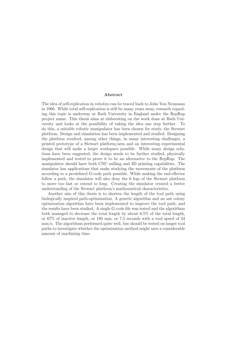
Abstract

The idea of self-replication in robotics can be traced back to John Von Neumannin 1966. While total self-replication is still be many years away, research regard-ing this topic is underway at Bath University in England under the RepRapproject name. This thesis aims at elaborating on the work done at Bath Uni-versity and looks at the possibility of taking the idea one step further. Todo this, a suitable robotic manipulator has been chosen for study, the Stewartplatform. Design and simulation has been implemented and studied. Designingthe platform resulted, among other things, in many interesting challenges, aprinted prototype of a Stewart platform/arm and an interesting experimentaldesign that will make a larger workspace possible. While many design solu-tions have been suggested, the design needs to be further studied, physicallyimplemented and tested to prove it to be an alternative to the RepRap. Themanipulator should have both CNC milling and 3D printing capabilities. Thesimulator has applications that make studying the movements of the platformaccording to a predefined G-code path possible. While making the end-effectorfollow a path, the simulator will also deny the 6 legs of the Stewart platformto move too fast or extend to long. Creating the simulator created a betterunderstanding of the Stewart platform’s mathematical characteristics.

Another aim of this thesis is to shorten the length of the tool path usingbiologically inspired path-optimization. A genetic algorithm and an ant colonyoptimization algorithm have been implemented to improve the tool path, andthe results have been studied. A single G-code file was tested and the algorithmsboth managed to decrease the total length by about 6.5% of the total length,or 67% of inactive length, or 180 mm, or 7.5 seconds with a tool speed of 24mm/s. The algorithms performed quite well, but should be tested on longer toolpaths to investigate whether the optimization method might save a considerableamount of machining time.

AcknowledgementsThis thesis has allowed me to explore the very interesting topic of robotics. Forthis, I wish to thank the Robotics and Intelligent Systems (ROBIN) researchgroup. They have enabled me to study some of the most interesting fields I haveexperienced in my academic endeavors.

I wish to thank my two supervisors, Mats Høvin and Kyrre Glette for guid-ance, but also for allowing me the freedom to influence the choice of topic toa large degree. Head engineer at ROBIN, Yngve Hafting, deserves thanks forhelping me with the practical challenges in creating printable designs and using3D printer software.

I also wish to thank my two closest peers at the University, Magnus Langeand Akbar Faghihi Moghaddam (Shahab) for insightful discussions and usefultips. Last but not least, deserving the biggest appreciation is my Anne-Catherinfor her patience during my late nights at the lab.

2

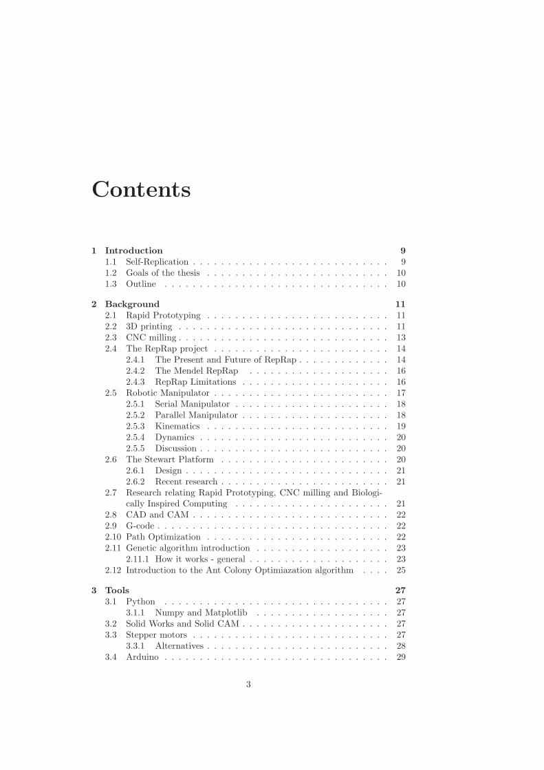
Contents

1 Introduction 91.1 Self-Replication . . . . . . . . . . . . . . . . . . . . . . . . . . . . 91.2 Goals of the thesis . . . . . . . . . . . . . . . . . . . . . . . . . . 101.3 Outline . . . . . . . . . . . . . . . . . . . . . . . . . . . . . . . . 10

2 Background 112.1 Rapid Prototyping . . . . . . . . . . . . . . . . . . . . . . . . . . 112.2 3D printing . . . . . . . . . . . . . . . . . . . . . . . . . . . . . . 112.3 CNC milling . . . . . . . . . . . . . . . . . . . . . . . . . . . . . . 132.4 The RepRap project . . . . . . . . . . . . . . . . . . . . . . . . . 14

2.4.1 The Present and Future of RepRap . . . . . . . . . . . . . 142.4.2 The Mendel RepRap . . . . . . . . . . . . . . . . . . . . 162.4.3 RepRap Limitations . . . . . . . . . . . . . . . . . . . . . 16

2.5 Robotic Manipulator . . . . . . . . . . . . . . . . . . . . . . . . . 172.5.1 Serial Manipulator . . . . . . . . . . . . . . . . . . . . . . 182.5.2 Parallel Manipulator . . . . . . . . . . . . . . . . . . . . . 182.5.3 Kinematics . . . . . . . . . . . . . . . . . . . . . . . . . . 192.5.4 Dynamics . . . . . . . . . . . . . . . . . . . . . . . . . . . 202.5.5 Discussion . . . . . . . . . . . . . . . . . . . . . . . . . . . 20

2.6 The Stewart Platform . . . . . . . . . . . . . . . . . . . . . . . . 202.6.1 Design . . . . . . . . . . . . . . . . . . . . . . . . . . . . . 212.6.2 Recent research . . . . . . . . . . . . . . . . . . . . . . . . 21

2.7 Research relating Rapid Prototyping, CNC milling and Biologi-cally Inspired Computing . . . . . . . . . . . . . . . . . . . . . . 21

2.8 CAD and CAM . . . . . . . . . . . . . . . . . . . . . . . . . . . . 222.9 G-code . . . . . . . . . . . . . . . . . . . . . . . . . . . . . . . . . 222.10 Path Optimization . . . . . . . . . . . . . . . . . . . . . . . . . . 222.11 Genetic algorithm introduction . . . . . . . . . . . . . . . . . . . 23

2.11.1 How it works - general . . . . . . . . . . . . . . . . . . . . 232.12 Introduction to the Ant Colony Optimiazation algorithm . . . . 25

3 Tools 273.1 Python . . . . . . . . . . . . . . . . . . . . . . . . . . . . . . . . 27

3.1.1 Numpy and Matplotlib . . . . . . . . . . . . . . . . . . . 273.2 Solid Works and Solid CAM . . . . . . . . . . . . . . . . . . . . . 273.3 Stepper motors . . . . . . . . . . . . . . . . . . . . . . . . . . . . 27

3.3.1 Alternatives . . . . . . . . . . . . . . . . . . . . . . . . . . 283.4 Arduino . . . . . . . . . . . . . . . . . . . . . . . . . . . . . . . . 29

3

4 Design 314.1 Actuator . . . . . . . . . . . . . . . . . . . . . . . . . . . . . . . . 314.2 CAD Design of the Stewart platform . . . . . . . . . . . . . . . . 334.3 First design . . . . . . . . . . . . . . . . . . . . . . . . . . . . . . 33

4.3.1 Motor housing . . . . . . . . . . . . . . . . . . . . . . . . 354.3.2 Nut housing . . . . . . . . . . . . . . . . . . . . . . . . . . 354.3.3 The universal joints . . . . . . . . . . . . . . . . . . . . . 364.3.4 The platform . . . . . . . . . . . . . . . . . . . . . . . . . 38

4.4 Prototype design . . . . . . . . . . . . . . . . . . . . . . . . . . . 404.5 Experimental design . . . . . . . . . . . . . . . . . . . . . . . . . 41

4.5.1 Discussion on version 3 . . . . . . . . . . . . . . . . . . . 434.6 Comparison with the RepRap . . . . . . . . . . . . . . . . . . . . 434.7 Concluding discussion . . . . . . . . . . . . . . . . . . . . . . . . 47

5 Simulator 495.1 Uses for the simulator . . . . . . . . . . . . . . . . . . . . . . . . 495.2 Mathematics for the Stewart platform . . . . . . . . . . . . . . . 50

5.2.1 Homogenous Transformation . . . . . . . . . . . . . . . . 515.3 Parsing G-code . . . . . . . . . . . . . . . . . . . . . . . . . . . . 525.4 Results . . . . . . . . . . . . . . . . . . . . . . . . . . . . . . . . . 54

5.4.1 Simple move simulation . . . . . . . . . . . . . . . . . . . 555.4.2 G-code simulation . . . . . . . . . . . . . . . . . . . . . . 555.4.3 Comment . . . . . . . . . . . . . . . . . . . . . . . . . . . 57

5.5 Concluding discussion . . . . . . . . . . . . . . . . . . . . . . . . 59

6 Biologically Inspired Path-Optimization 616.1 Research method . . . . . . . . . . . . . . . . . . . . . . . . . . . 616.2 Parsing G-code . . . . . . . . . . . . . . . . . . . . . . . . . . . . 636.3 Test data . . . . . . . . . . . . . . . . . . . . . . . . . . . . . . . 636.4 Genetic Algorithm . . . . . . . . . . . . . . . . . . . . . . . . . . 65

6.4.1 How it works - specific . . . . . . . . . . . . . . . . . . . . 656.4.2 Results for the Genetic Algorithm . . . . . . . . . . . . . 686.4.3 Discussion on GA test results . . . . . . . . . . . . . . . . 71

6.5 Ant Colony Optimization . . . . . . . . . . . . . . . . . . . . . . 746.5.1 Applying ACO to the TSP . . . . . . . . . . . . . . . . . 746.5.2 Results for the Ant System . . . . . . . . . . . . . . . . . 756.5.3 Discussion on ACO test results . . . . . . . . . . . . . . . 78

6.6 Concuding discussion on Tool path-optimization . . . . . . . . . 816.6.1 Comparing genetic algorithm and ant colony system . . . 816.6.2 General discussion . . . . . . . . . . . . . . . . . . . . . . 82

7 Conclusion and proposals for further work 857.1 Conclusion . . . . . . . . . . . . . . . . . . . . . . . . . . . . . . 857.2 Further Work . . . . . . . . . . . . . . . . . . . . . . . . . . . . . 86References . . . . . . . . . . . . . . . . . . . . . . . . . . . . . . . . . . 89

A Code attachment 95A.1 Simulation software . . . . . . . . . . . . . . . . . . . . . . . . . . 95A.2 Biologically Inspired Path-optimization . . . . . . . . . . . . . . 115

4

List of Figures

2.1 Illustration of a 3D printer . . . . . . . . . . . . . . . . . . . . . . 122.2 Illustration of a Milling Machine . . . . . . . . . . . . . . . . . . 132.3 A traditional commercial milling machine[49] . . . . . . . . . . . 142.4 The Tricept 9000 . . . . . . . . . . . . . . . . . . . . . . . . . . . 152.5 The latest generation RepRap, the Mendel[45] . . . . . . . . . . . 152.6 A pictute of the Hydra combined CNC milling machine and 3D

printer [52] . . . . . . . . . . . . . . . . . . . . . . . . . . . . . . 172.7 A serial manipulator with six revolute joints. . . . . . . . . . . . 182.8 A 3 legged parallel manipulator. . . . . . . . . . . . . . . . . . . 192.9 A cost matrix of a undirected complete graph with four nodes

(cities). . . . . . . . . . . . . . . . . . . . . . . . . . . . . . . . . 232.10 Flowchart of general evolutionary algorithm. . . . . . . . . . . . . 24

3.1 A stepper motor . . . . . . . . . . . . . . . . . . . . . . . . . . . 283.2 The Arduino Mega . . . . . . . . . . . . . . . . . . . . . . . . . . 29

4.1 An illustration of the rapid prototyping system . . . . . . . . . . 324.2 A CAD model of the actuator . . . . . . . . . . . . . . . . . . . . 334.3 A CAD model of the actuator, whole and cut in half . . . . . . . 344.4 CAD model of the first design of the entire Stewart platform . . 354.5 CAD model of the motorhousing . . . . . . . . . . . . . . . . . . 364.6 The nut housing (top part of the arm) for the Stewart platform,

first designs . . . . . . . . . . . . . . . . . . . . . . . . . . . . . . 374.7 Limitation of tilt in the Stewart platform . . . . . . . . . . . . . 374.8 A picture of a universial joint [48] . . . . . . . . . . . . . . . . . . 384.9 The universal joints . . . . . . . . . . . . . . . . . . . . . . . . . 384.10 Alternatives for the universal joint . . . . . . . . . . . . . . . . . 394.11 A CAD model of the platform . . . . . . . . . . . . . . . . . . . . 394.12 The prototype of an arm printed on a commercial 3D printer . . 404.13 The parts of the prototype of an arm printed on a commercial

3D printer . . . . . . . . . . . . . . . . . . . . . . . . . . . . . . . 414.14 Exploded view of the motorhousing and of the platform connector

for the prototype design . . . . . . . . . . . . . . . . . . . . . . . 424.15 CAD models of the nut housing for the prototype version . . . . 424.16 A layer of deposited material in the professional 3D printing soft-

ware, Catalyst EX. . . . . . . . . . . . . . . . . . . . . . . . . . . 434.17 Experimental design, version 1 . . . . . . . . . . . . . . . . . . . 444.18 Experimental design, version 2 . . . . . . . . . . . . . . . . . . . 444.19 Experimental design, version 3 . . . . . . . . . . . . . . . . . . . 45

5

4.20 Close up of version 3 . . . . . . . . . . . . . . . . . . . . . . . . . 454.21 Crash in threaded rods for experimental design 3. 1000 mm

threaded rods. . . . . . . . . . . . . . . . . . . . . . . . . . . . . 464.22 No crash with experimental design 3. Showing a large tilt in the

moving platform. . . . . . . . . . . . . . . . . . . . . . . . . . . . 47

5.1 These are the dimensions for the base platform . . . . . . . . . . 505.2 These are the dimensions for the top platform . . . . . . . . . . . 515.3 The path created for testing simple move . . . . . . . . . . . . . 555.4 The simulation of the simple move . . . . . . . . . . . . . . . . . 565.5 The path extracted from G-code, seen from above . . . . . . . . 575.6 The path extracted from G-code, seen from the side . . . . . . . 585.7 The part of the path used for simulation . . . . . . . . . . . . . . 585.8 Simulation of the G-code with a fast speed of 30 mm/s and slow

speed of 15 mm/s. . . . . . . . . . . . . . . . . . . . . . . . . . . 59

6.1 A plaque reading CNC taken from [20] . . . . . . . . . . . . . . . 636.2 3 cities and the paths between them . . . . . . . . . . . . . . . . 646.3 PMX 1 . . . . . . . . . . . . . . . . . . . . . . . . . . . . . . . . . 676.4 PMX 2 . . . . . . . . . . . . . . . . . . . . . . . . . . . . . . . . . 676.5 PMX 3 . . . . . . . . . . . . . . . . . . . . . . . . . . . . . . . . . 676.6 Correcting the edges. . . . . . . . . . . . . . . . . . . . . . . . . . 686.7 Inversion mutation . . . . . . . . . . . . . . . . . . . . . . . . . . 686.8 Correcting the edges after mutation . . . . . . . . . . . . . . . . 686.9 The Mean best vs the Average number of evaluations for the GA 716.10 The best individual for each generation using parameter setting

4 in table 6.1 and 150 generations (genetic algorithm) . . . . . . 726.11 The best individual for each generation using parameter setting

5 in table 6.1 and 50 genereations (genetic algorithm) . . . . . . 736.12 The Mean best vs the Average number of evaluations for the Ant

System. . . . . . . . . . . . . . . . . . . . . . . . . . . . . . . . . 786.13 The best individual for each generation using parameter setting

1 in table 6.3(ant system) . . . . . . . . . . . . . . . . . . . . . . 806.14 The best individual for each generation using parameter setting

1 in table 6.3 and 500 generations(ant system) . . . . . . . . . . 806.15 The best individual for each generation using parameter setting

1 in table 6.3 and 50 ants(ant system) . . . . . . . . . . . . . . . 81

6

List of Tables

2.1 Specifiactions for the Mendel RepRap [57] . . . . . . . . . . . . . 16

5.1 Interpreted G-code [54] . . . . . . . . . . . . . . . . . . . . . . . 53

6.1 Parameter settings for the different tests. . . . . . . . . . . . . . 696.2 Test results for different parameter settings for the genetic algo-

rithm. . . . . . . . . . . . . . . . . . . . . . . . . . . . . . . . . . 706.3 Parameter settings for the different tests . . . . . . . . . . . . . . 766.4 Test results for different parameter settings for the ant colony

optimization algorithm . . . . . . . . . . . . . . . . . . . . . . . . 77

7

Abbreviations

CNC - Computer Numerically Controlled

RepRap - replicating rapid prototyper

CAD - Computer Aided Design

CAM - Computer aided Manufacturing

DOF - degrees of freedom

PM - parallel manipulator

SM - serial manipulator

R - rotational joint

P - prismatic joint

U - universal joint

TSP - Traveling Salesman Problem

FDM - Fused Deposition Modeling

LOM - Laminated Object Manufacturing

SLS - Selective Laser Sintering

STL - Stereolithography

PKM - Parallel Kinematics Machine

FFF - Fused Filament Fabrication

PNG - Portable Network Graphics

FPS - Frames per second

SUS - Stochastic Universal Sampling

PMX - Partially Mapped Crossover

ACO - Ant Colony Optimization

8

Chapter 1

Introduction

3D printing and CNC milling have been around for a long time and have tosome extent even reached the consumer market.[61, 38] In the industry, 3Dprinting and sometimes CNC milling are used to create prototypes in a quick andcost effective manner. For the hobbyist (or amateur), the use is more directedtowards creating almost anything, including prototypes, a building set for anRC airplane, parts for a robot, a box-container or simply a spoon. This thesisfocuses on the hobby aspect of 3D printing and CNC milling that translatesinto some keywords that are vital to be maintained: affordability, simplicity,open-source and size. These are in addition to those common to 3D printingand CNC milling such as accuracy, rigidity (especially for CNC milling), speedand time.

This thesis has one foot planted in the theoretical world of path-optimization,kinematics and simulation. And the other foot planted in the practical worldof design, motors and electronics. Both of these aspects have been explored asthey are both essential for the development of a robot manipulator.

1.1 Self-Replication

The idea of self-replication of non-biological entities was first introduced by Johnvon Neumann in the late 40s with a thought experiment and later published inthe 1960s.[7] The concept of self-replication for biological entities is as old as lifeand it is what life is based on as all living creatures replicate themselves. Onewell developed project based on self-replication of non-biological entities is theRepRap project.

With self-replication there are, as I see it, two ways to go, simplicity orcomplexity. The complex viewpoint results in a large machine, or even anautonomous factory, capable of producing almost anything. This is an areathat is very costly and thus hard to research. The simple aspect is to startwith a simple machine and try to make it create parts of itself. This is whatthe people at Bath University have done with their RepRap project. RepRapis short for Replicating Rapid Prototyper and is basically a small 3D printerthat is quite affordable. As the machine is so mechanically simple, the challengeis to make it able to do more things without sacrificing its simplicity. For ahighly complex machine the challenge would have been the opposite, to make

9

it simpler without sacrificing functionality.

1.2 Goals of the thesis

With the RepRap project as a stepping stone, this thesis will mainly investigatethe possibilities of increasing functionality without sacrificing simplicity. Todo this, a type robotic manipulator has to be chosen and studied. Thus, theentry point of this thesis is the hobby world of 3D printing and CNC milling,exemplified with the RepRap project. To study the robotic manipulator, threegoals have been created:

1. Create and compare a new design with the RepRap 3D printer developedat Bath University, England. The new design should be an improvementin certain fields as discussed in chapter 2.4.3.

2. Create a simulator to explore the robot manipulator and allow furtherexperiments.

3. Look at the tool path-optimization (minimizing the length of the toolpath) problem and implement biologically inspired algorithms to solve it.

The tool path-optimization problem has been included for two reasons. Itis relevant to 3D printing and CNC milling, shortening the tool path will alsoshorten operation time. Secondly, it is an interesting research topic that hasreceived attention lately. See chapter 2.7 for a discussion. The three goalssuggest different approaches to the world of the robotic manipulator. It isbelieved that this will give a better insight as several aspects gets highlighted.

1.3 Outline

As mentioned, the thesis is more or less divided in three; however the three topicsoverlap each other in many areas and are connected. After the introduction, thethesis continues with a chapter on the background of the different topics. Also,based on a discussion, the Stewart platform is chosen as the robotic manipulatorto study. The next chapter, Tools, deal with the different tools used in the threemain chapters, Design, Simulator and Biologically Inspired Path-Optimization.The Design chapter presents different designs created with CAD software anddiscusses many aspects relating the realization of the designs and how the designcompare to the RepRap. The next chapter, Simulation, moves a bit away fromthe practical world and investigates some mathematical theories behind theStewart platform. Also, to implement the simulator, G-code is studied and aG-code parser is created. The tool path length is tried to be shortened in thechapter on biologically inspired path-optimization. The movements where thetool is inactive are studied and two algorithms are implemented and tested witha G-code file. The results from the tests are discussed and the applicabilityof the algorithm and type of path-optimization is assessed. The final chapterconcludes the three main chapters and tries to use the experience from them todecide whether the Stewart platform as presented can be an alternative to theRepRap. Further work is also discussed in the last chapter.

10

Chapter 2

Background

Much of the background theory is presented in this chapter. Also, some discus-sion regarding central aspects of this thesis is made. First, rapid prototyping,3D printing and CNC milling are introduced. Then, the RepRap project is de-scribed and discussed. After that the types of robotic manipulator is exploredand the one to be studied in this thesis is chosen. The chosen manipulatoris further presented, exploring the relating research. The areas of CAD andCAM, G-code and path-optimization are then introduced. Finally, the geneticalgorithm and the ant colony optimization are introduced.

2.1 Rapid Prototyping

Rapid prototyping is a way to create an inexpensive prototype directly andfast. Descriptions of the components are created on a computer and then di-rectly manufactured.[6] Also, instead of creating the whole design, simplifica-tions and/or miniatures of the final prototype can be created. This is often veryuseful in the designing stages of different engineering tasks.

Two of the methods used for rapid prototyping are 3D printing and millingwith CNC milling machine. There are several different types of each, from thesimplest hobby version to multi million commercial ones. A more advancedtype of rapid prototyping is used to work with hard metals and to enhance theaccuracy and quality. This technology is very expensive and outside the scopeof this thesis. Other deposition based manufacturing methods than 3D print-ing (or fused filament fabrication) include Stereolithography, Fused DepositionModeling (FDM), Laminated Object Manufacturing (LOM) and Selective LaserSintering (SLS).[27] The different technologies used for depositing the materialis outside the scope of this thesis, and have not been studied in detail.

2.2 3D printing

As mentioned, there are many different types of 3D printers. To keep insidethe scope of the this text, mainly a simplified description of the 3D printingtechnology used at Bath University for their RepRap project will described(FFF - Fused Filament Fabrication). This technology uses an extruder thatmelts a material and then extrudes the material onto a board. The material

11

is often a type of polymer, for example ABS (the “Lego-brick polymer”) ornylon.[6] The board and/or the extruder can move in the xyz-planes to build 3-dimensional objects. Every layer is held together because of the characteristicsthe material has when it is hot. It is called 3D printing because it is quitesimilar to the more regular 2D printing that is used for printing on paper.

z

x

y

The extruder

The part

Hole

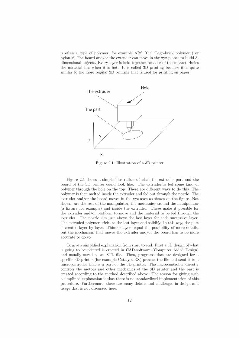
Figure 2.1: Illustration of a 3D printer

Figure 2.1 shows a simple illustration of what the extruder part and theboard of the 3D printer could look like. The extruder is fed some kind ofpolymer through the hole on the top. There are different ways to do this. Thepolymer is then melted inside the extruder and fed out through the nozzle. Theextruder and/or the board moves in the xyz-axes as shown on the figure. Notshown, are the rest of the manipulator, the mechanics around the manipulator(a fixture for example) and inside the extruder. These make it possible forthe extruder and/or platform to move and the material to be fed through theextruder. The nozzle sits just above the last layer for each successive layer.The extruded polymer sticks to the last layer and solidify. In this way, the partis created layer by layer. Thinner layers equal the possibility of more details,but the mechanism that moves the extruder and/or the board has to be moreaccurate to do so.

To give a simplified explanation from start to end: First a 3D design of whatis going to be printed is created in CAD-software (Computer Aided Design)and usually saved as an STL file. Then, programs that are designed for aspecific 3D printer (for example Catalyst EX) process the file and send it to amicrocontroller that is a part of the 3D printer. The microcontroller directlycontrols the motors and other mechanics of the 3D printer and the part iscreated according to the method described above. The reason for giving sucha simplified explanation is that there is no standardized implementation of thisprocedure. Furthermore, there are many details and challenges in design andusage that is not discussed here.

12

2.3 CNC milling

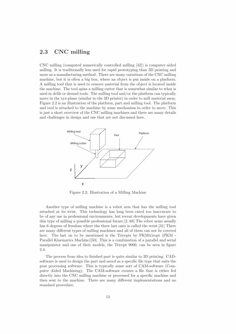
CNC milling (computed numerically controlled milling [42]) is computer aidedmilling. It is traditionally less used for rapid prototyping than 3D printing andmore as a manufacturing method. There are many variations of the CNC millingmachine, but it is often a big box, where an object is put inside on a platform.A milling tool that is used to remove material from the object is located insidethe machine. The tool spins a milling cutter that is somewhat similar to what isused in drills or dremel tools. The milling tool and/or the platform can typicallymove in the xyz-plane (similar to the 3D printer) in order to mill material away.Figure 2.2 is an illustration of the platform, part and milling tool. The platformand tool is attached to the machine by some mechanism in order to move. Thisis just a short overview of the CNC milling machines and there are many detailsand challenges in design and use that are not discussed here.

z

x

y

Milling tool

Milling cutter

PartPlatform

Figure 2.2: Illustration of a Milling Machine

Another type of milling machine is a robot arm that has the milling toolattached at its wrist. This technology has long been rated too inaccurate tobe of any use in professional environments, but recent developments have giventhis type of milling a possible professional future.[2, 68] The robot arms usuallyhas 6 degrees of freedom where the three last ones is called the wrist.[31] Thereare many different types of milling machines and all of them can not be coveredhere. The last on to be mentioned is the Tricepts by PKMtricept (PKM -Parallel Kinematics Machine)[50]. This is a combination of a parallel and serialmanipulator and one of their models, the Tricept 9000, can be seen in figure2.4.

The process from idea to finished part is quite similar to 3D printing. CAD-software is used to design the part and saved as a specific file type that suits thepost processing software. This is typically some sort of CAM-software (Com-puter Aided Machining). The CAM-software creates a file that is either feddirectly into the CNC milling machine or processed for a specific machine andthen sent to the machine. There are many different implementations and nostandard procedure.

13

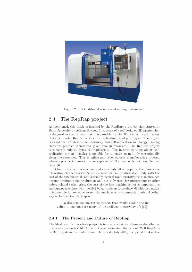
Figure 2.3: A traditional commercial milling machine[49]

2.4 The RepRap project

As mentioned, this thesis is inspired by the RepRap, a project that started atBath University by Adrian Bowyer. It consists of a self designed 3D printer thatis designed in such a way that it is possible for the 3D printer to print manyof its own parts. RepRap is short for replicating rapid prototyper. The projectis based on the ideas of self-assembly and self-replication in biology. Livingcreatures produce themselves, given enough resources. The RepRap projectis currently only studying self-replication. The interesting thing about self-replication is that it makes it possible for an entity to multiply exceptionallygiven the resources. This is unlike any other current manufacturing process,where a production growth in an exponential like manner is not possible overtime. [6]

Behind the idea of a machine that can create all of its parts, there are someinteresting characteristics. Since the machine can produce itself, only with thecost of the raw materials and assembly, typical rapid prototyping machines canbecome profitable for production and not only used for prototyping or otherhobby related tasks. Also, the cost of the first machine is not as important assubsequent machines will (ideally) be quite cheap to produce.[6] This also makesit impossible for someone to sell the machine on a commercial basis. Anotherway to look at the RepRap is:

...a desktop manufacturing system that would enable the indi-vidual to manufacture many of the artifacts in everyday life [69]

2.4.1 The Present and Future of RepRap

The ideal goal for the whole project is to create what von Neuman describes asuniversal constructor.[51] Adrian Bowyer estimated that about 2500 RepRapsor RepRap deviates exists around the world (July 2009) compared to 4 at the

14

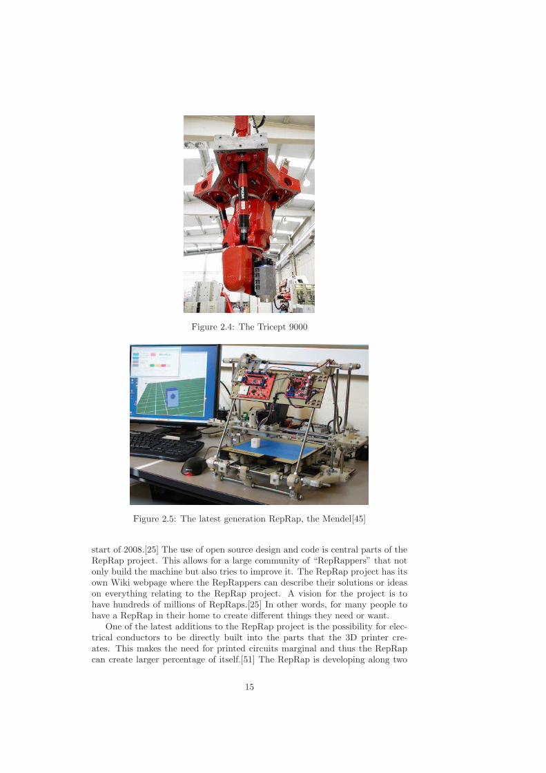
Figure 2.4: The Tricept 9000

Figure 2.5: The latest generation RepRap, the Mendel[45]

start of 2008.[25] The use of open source design and code is central parts of theRepRap project. This allows for a large community of “RepRappers” that notonly build the machine but also tries to improve it. The RepRap project has itsown Wiki webpage where the RepRappers can describe their solutions or ideason everything relating to the RepRap project. A vision for the project is tohave hundreds of millions of RepRaps.[25] In other words, for many people tohave a RepRap in their home to create different things they need or want.

One of the latest additions to the RepRap project is the possibility for elec-trical conductors to be directly built into the parts that the 3D printer cre-ates. This makes the need for printed circuits marginal and thus the RepRapcan create larger percentage of itself.[51] The RepRap is developing along two

15

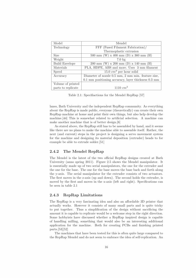
Model MendelTechnology FFF (Fused Filament Fabrication)/

Thermoplastic extrusionSize 500 mm (W) x 400 mm (D) x 360 mm (H)Weight 7.0 kgBuild Envelope 200 mm (W) x 200 mm (D) x 140 mm (H)Materials PLA, HDPE, ABS and more. Uses 3 mm filamentSpeed 15.0 cm3 per hour solidAccuracy Diameter of nozzle 0.5 mm, 2 mm min. feature size,

0.1 mm positioning accuracy, layer thickness 0.3 mmVolume of printedparts to replicate 1110 cm3

Table 2.1: Specifiactions for the Mendel RepRap [57]

lanes, Bath University and the independent RepRap community. As everythingabout the RepRap is made public, everyone (theoretically) can create their ownRepRap machine at home and print their own things, but also help develop themachine.[44] This is somewhat related to artificial selection. A machine canmake another machine that is of better design.[6]

As stated above, the RepRap still has to be assembled by hand, and it seemslike there are no plans to make the machine able to assemble itself. Rather, thenext (and current) steps in the project is designing a servo movement systemfor the machine and designing its material deposition (extruder) heads to forexample be able to extrude solder.[51]

2.4.2 The Mendel RepRap

The Mendel is the latest of the two official RepRap designs created at BathUniversity (anno spring 2011). Figure 2.5 shows the Mendel manipulator. Itis essentially made up of two serial manipulators, the one for the extruder andthe one for the base. The one for the base moves the base back and forth alongthe y-axis. The serial manipulator for the extruder consists of two actuators.The first moves in the z-axis (up and down). The second holds the extruder, ismoved by the first and moves in the x-axis (left and right). Specifications canbe seen in table 2.1

2.4.3 RepRap Limitations

The RepRap is a very fascinating idea and also an affordable 3D printer thatactually works. However it consists of many small parts and is quite trickyto put together. Thus a simplification of the design without sacrificing theamount it is capable to replicate would be a welcome step in the right direction.Some hobbyists have discussed whether a RepRap inspired design is capableof handling milling, something that would also be an interesting additionalapplication for the machine. Both for creating PCBs and finishing printedparts.[53][52]

The machines that have been tested for this is often quite large compared tothe RepRap Mendel and do not seem to embrace the idea of self-replication. An

16

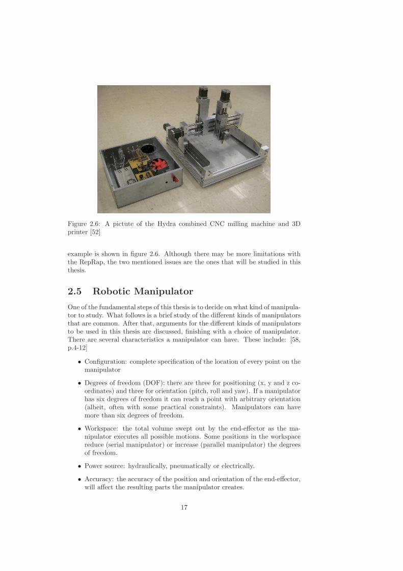
Figure 2.6: A pictute of the Hydra combined CNC milling machine and 3Dprinter [52]

example is shown in figure 2.6. Although there may be more limitations withthe RepRap, the two mentioned issues are the ones that will be studied in thisthesis.

2.5 Robotic Manipulator

One of the fundamental steps of this thesis is to decide on what kind of manipula-tor to study. What follows is a brief study of the different kinds of manipulatorsthat are common. After that, arguments for the different kinds of manipulatorsto be used in this thesis are discussed, finishing with a choice of manipulator.There are several characteristics a manipulator can have. These include: [58,p.4-12]

• Configuration: complete specification of the location of every point on themanipulator

• Degrees of freedom (DOF): there are three for positioning (x, y and z co-ordinates) and three for orientation (pitch, roll and yaw). If a manipulatorhas six degrees of freedom it can reach a point with arbitrary orientation(albeit, often with some practical constraints). Manipulators can havemore than six degrees of freedom.

• Workspace: the total volume swept out by the end-effector as the ma-nipulator executes all possible motions. Some positions in the workspacereduce (serial manipulator) or increase (parallel manipulator) the degreesof freedom.

• Power source: hydraulically, pneumatically or electrically.

• Accuracy: the accuracy of the position and orientation of the end-effector,will affect the resulting parts the manipulator creates.

17

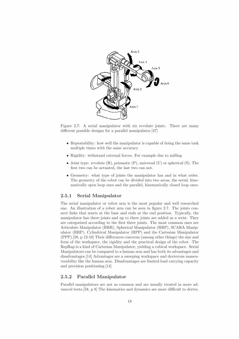
Figure 2.7: A serial manipulator with six revolute joints. There are manydifferent possible designs for a parallel manipulator.[47]

• Repeatability: how well the manipulator is capable of doing the same taskmultiple times with the same accuracy

• Rigidity: withstand external forces. For example due to milling

• Joint type: revolute (R), prismatic (P), universal (U) or spherical (S). Thefirst two can be actuated, the last two can not.

• Geometry: what type of joints the manipulator has and in what order.The geometry of the robot can be divided into two areas, the serial, kine-matically open loop ones and the parallel, kinematically closed loop ones.

2.5.1 Serial Manipulator

The serial manipulator or robot arm is the most popular and well researchedone. An illustration of a robot arm can be seen in figure 2.7. The joints con-nect links that starts at the base and ends at the end position. Typically, themanipulator has three joints and up to three joints are added as a wrist. Theyare categorized according to the first three joints. The most common ones areArticulate Manipulator (RRR), Spherical Manipulator (RRP), SCARA Manip-ulator (RRP), Cylindrical Manipulator (RPP) and the Cartesian Manipulator(PPP).[58, p 12-18] Their differences concerns (among other things) the size andform of the workspace, the rigidity and the practical design of the robot. TheRepRap is a kind of Cartesian Manipulator, yielding a cubical workspace. SerialManipulators can be compared to a human arm and has both its advantages anddisadvantages.[14] Advantages are a sweeping workspace and dexterous maneu-verability like the human arm. Disadvantages are limited load carrying capacityand precision positioning.[14]

2.5.2 Parallel Manipulator

Parallel manipulators are not as common and are usually treated in more ad-vanced texts.[58, p 8] The kinematics and dynamics are more difficult to derive,

18

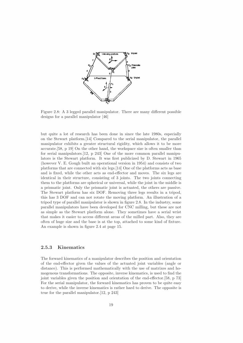
Figure 2.8: A 3 legged parallel manipulator. There are many different possibledesigns for a parallel manipulator [46]

but quite a lot of research has been done in since the late 1980s, especiallyon the Stewart platform.[14] Compared to the serial manipulator, the parallelmanipulator exhibits a greater structural rigidity, which allows it to be moreaccurate.[58, p 19] On the other hand, the workspace size is often smaller thanfor serial manipulators.[12, p 243] One of the more common parallel manipu-lators is the Stewart platform. It was first publicized by D. Stewart in 1965(however V. E. Gough built an operational version in 1954) and consists of twoplatforms that are connected with six legs.[14] One of the platforms acts as baseand is fixed, while the other acts as end-effector and moves. The six legs areidentical in their structure, consisting of 3 joints. The two joints connectingthem to the platforms are spherical or universal, while the joint in the middle isa prismatic joint. Only the prismatic joint is actuated, the others are passive.The Stewart platform has six DOF. Removing three legs results in a tripod,this has 3 DOF and can not rotate the moving platform. An illustration of atripod type of parallel manipulator is shown in figure 2.8. In the industry, someparallel manipulators have been developed for CNC milling, but these are notas simple as the Stewart platform alone. They sometimes have a serial wristthat makes it easier to access different areas of the milled part. Also, they areoften of huge size and the base is at the top, attached to some kind of fixture.An example is shown in figure 2.4 at page 15.

2.5.3 Kinematics

The forward kinematics of a manipulator describes the position and orientationof the end-effector given the values of the actuated joint variables (angle ordistance). This is performed mathematically with the use of matrixes and ho-mogenous transformations. The opposite, inverse kinematics, is used to find thejoint variables given the position and orientation of the end-effector.[58, p 73]For the serial manipulator, the forward kinematics has proven to be quite easyto derive, while the inverse kinematics is rather hard to derive. The opposite istrue for the parallel manipulator.[12, p 243]

19

2.5.4 Dynamics

The dynamics is used to perform an in depth analysis of manipulator move-ment and includes a study of the forces and torques. For example, the frictionin joints can be included in a dynamic model. The dynamics for parallel ma-nipulators are very advanced, while for serial manipulators they are somewhatmore simple.[14] However, dynamics are outside the scope of this thesis and willnot be considered.

2.5.5 Discussion

One of the basic ideas behind this thesis is to improve the RepRap concept’scapabilities to be alternatively equipped with a milling tool to perform millingand an extruder to print in 3D. To do this, the tool can be changed allowing themanipulator to both print and mill the same part. For this to be possible themanipulator must have some additional characteristics as opposed to be ableto do only one of the things. An important issue is that milling requires muchmore structure rigidity than 3D printing.

To be able to perform 3D printing a manipulator should have 3 DOF. In or-der to mill the manipulator should have at least 3 DOF, preferably more. Theworkspace should be as large as possible. Electrical power source is preferableas pneumatic is too inaccurate and hydraulic require much maintenance, lot ofperipheral equipment and is very noisy. Accuracy and repeatability is impor-tant both for 3D printing and milling, and rigidity is as mentioned especiallyimportant for milling.

Considering the greater structural rigidity of the parallel manipulator, it ismore suitable for milling than a serial manipulator. On the other hand, theworkspace is smaller, limiting the size of parts created. For both 3D printingand CNC milling the end-effector location and orientation is always known. Thiscalls for the use of inverse kinematics that is simple for the Stewart platform.

An important aspect is that the robot should be an alternative to theRepRap. This means that the design limitations given by the RepRap conceptshould be paramount in the design process. The most important limitations arethat the design can not be too advanced or too expensive as the robot is to beavailable to as many as possible. And that the robot should consist of as manyas possible parts that it can create itself.

Taking these arguments into account and considering the interesting recentresearch in the field, the Stewart platform was deemed the most suitable plat-form for hobby oriented 3D printing and milling and thus chosen for this thesis.

2.6 The Stewart Platform

Bhaskar Dasgupta and T.S Mruthyunjaya have studied the research develop-ment of the Stewart platform per 1998.[14] They report that an increasingamount of research on the platform has been done in the 80s and 90s. Themain focus of their article is the research areas and challenges of the Stew-art platform, but by doing so they also give a characterization of the Stewartplatform. Parallel manipulators like the Stewart platform are believed to havegreater rigidity and positioning capability than serial manipulators. The kine-matics (relation between length of legs and the position of the end-effector) is

20

opposite in difficulty to the serial manipulator. Inverse kinematics is simple(deciding the length of the legs given the position and orientation of the end-effector), while forward kinematics is complex and difficult. A similar dualityis reported when singularities are discussed. The Stewart platform experiencesingularities as configurations where the machine gains one degree of freedom,but looses its controllability. The issue of singularities, which is tough to dealwith, is not further investigated in this thesis. Another difficult domain in theStewart platform research is analyzing and determining the workspace. Theauthors present some interesting research on this difficult topic. This thesis willhowever only suggest that the workspace of a parallel manipulator is smallerthan the workspace of a serial manipulator of roughly the same size.

2.6.1 Design

Dasgupta and Mruthyunjaya present the generalized design of the Stewart plat-form as two platforms connected with six extensible legs. The legs are connectedwith spherical joints at both ends or spherical at one and universal at the other.The designs presented later in this thesis consist of universal joints at both ends.This is not entirely uncommon as the designs in these videos shows. [63] [62]

The shape of the platforms is quite arbitrary. The authors present amongother designs, a design where both base and top are triangles where legs meetin pairs at the edges (3-3) and one where the base has six distinct connectionpoints for the joints (6-3). The design presented later in this thesis use a 6-6type of design, where in position zero, the two platforms are hexagons rotated180 degrees in relation to each other.

2.6.2 Recent research

Much of the post 1998 research that was found dealt with the forward kinematicsof the Stewart platform. The issue with this problem is that it is complex andtime consuming to calculate. Several researchers have presented good solutionsto the problem,[67, 41, 35, 23, 15] and some even suggesting forward kinematicsapplications to be used in real-time.[32, 29]

Ilian A. Bonev and Jeha Ryu have studied a new method to find a set of allattainable orientations of the platform about a fixed point.[5] Yunjiang Lou et alhave studied the dynamic based trajectory planning for a Stewart platform.[36]Other studies of the dynamics has been performed as well. Denis Garagic andKrishnaswamy Srinivasan have studied friction compensation for the Stewartplatform.[21] Shih-Ming Wang and Korner F. Ehmann et al have studied errorand accuracy models and analysis of the Stewart platform.[66] Others havestudied robots that are similar to the Stewart platform.[70, 24]

2.7 Research relating Rapid Prototyping, CNC

milling and Biologically Inspired Computing

Some papers have discussed the use of Biologically Inspired Computing in re-lation to rapid prototyping, CNC milling or similar applications. Li Xueguanget al have established the Traveling Salesman Problem on the path-optimizationproblem and have applied the backtracking and genetic algorithm on the problem.[33]

21

Similarly, Ajay Joneja et al have in [27] studied tool path-optimization for therapid prototyping process with a genetic algorithm. Pang King Wah et al havedeveloped an enhanced genetic algorithm to solve the problem.[65] Z. Car etal have also used the genetic algorithm to optimize machining parameters in aturning process.[8] Similar research has been done for CNC rough machining byAgathocles A. Krimpenis et al.[30]

2.8 CAD and CAM

Mechanical CAD-software (Computer Aided Design) is a type of software wherea 3D design of a physical object is created by the user. CAD-software also hasmany options to for example test and assemble the created objects. All or mostof the characteristics of the object can be specified depending on the software.

Computer-aided manufacturing (CAM) is a set of techniques used in com-puter control for manufacturing.[13, p. 102] More concretely; it is the process ofinterpreting the design file from CAD software in order to create a file written inG-code or other similar control language. The file can be interpreted to controlCNC milling machines and 3D printers. The G-code file sometimes needs to bepost-processed in order to fit the specific manufacturing machine. With largersystems the post-processing can be integrated in the CAD and CAM software.

2.9 G-code

G-code is a very common language for CNC-programming, but it might alsorefer to a part of the CNC-programming, namely preparatory commands.[54,p47-48] In this thesis, G-code refer to the programming language and for ex-ample includes miscellaneous commands. The preparatory commands are usedto prepare the control system to a certain state of operation. Following thepreparatory commands (Gxx) are specific instructions for that type of com-mand. An example is G01, which means Linear Interpolation and is followedby the position and orientation the end-effector is going to move to.

The miscellaneous functions (Mxx) is used to command the tool,[54, p 52-53] it might for example start a milling tool in the clockwise direction (M03)or stop the program (M00). Miscellaneous functions are divided into machinerelated functions and program related functions. Machine related functions con-trols various physical operations of the CNC machine while the program relatedfunctions control the execution of a CNC program (such as calling and endinga subprogram). For preparatory and miscellaneous commands implemented inthis thesis see chapter 5.3, table 5.1.

2.10 Path Optimization

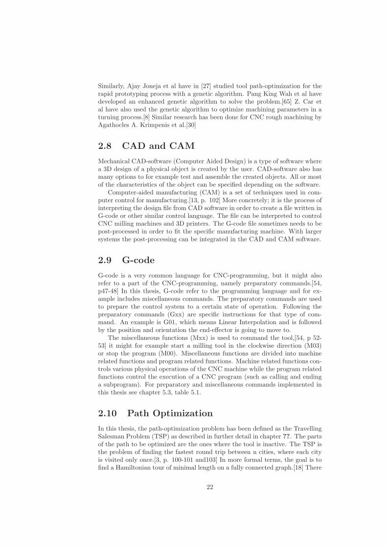
In this thesis, the path-optimization problem has been defined as the TravellingSalesman Problem (TSP) as described in further detail in chapter ??. The partsof the path to be optimized are the ones where the tool is inactive. The TSP isthe problem of finding the fastest round trip between n cities, where each cityis visited only once.[3, p. 100-101 and103] In more formal terms, the goal is tofind a Hamiltonian tour of minimal length on a fully connected graph.[18] There

22

0 32 15 532 0 63 2115 63 0 15 21 1 0

Figure 2.9: A cost matrix of a undirected complete graph with four nodes(cities).

are (n-1)! possible tours, therefore using the brute force algorithm for a graphwith more than 8-9 cities is infeasible.[3]

The TSP is a hard or NP-hard problem depending on how the problem ispresented. Currently, there exists no polynomial algorithm that solves the TSPand it is unlikely that such an algorithm ever will be found. The algorithms thatsolves the TSP are super polynomial (grows faster than any polynomial).[3] Tosolve the TSP, a cost matrix is used that presents the distances between all thecities. The algorithm searches this cost matrix to find the best solution. Anexample of a cost matrix is given in figure 2.9.

A thorough investigation of the research done in tool path-optimization withtraditional algorithms has not been done for this research. Limited investigationsuggests that the research has focused on making the CNC milling create bettersurface results on the parts that is milled. Two examples of this kind of researchcan be found in [39] and [4]. An article on optimizing the tool path length forturning CNC milling can be found in [65]. For studies of the problem done withbiologically inspired algorithms, see chapter 2.7.

2.11 Genetic algorithm introduction

The genetic algorithm is one of the first types of evolutionary algorithms andwas introduced by Holland in 1975.[19, p 2] It is inspired by the evolution ofliving organisms as seen in nature and by Charles Darwin’s theory of evolution.The two cornerstones of evolutionary computing are competition based progress(the survival of the fittest) and combination of genes during reproduction. Thecombination of genes can include mutation.[19, p 2-4] The advantage of emulat-ing this behavior on a computer is that the form and size of individuals is decidedby the programmer. Likewise is the way genes combine during reconstruction,what individuals survive for another generation and so on. Evolutionary com-puting has proved to be suitable to solve several problems. Examples of realworld applications are the timetabling of universities and design of a satellitedish holder boom. The boom proved to be 20 000% better than the traditionalshape.[19, p 10]

2.11.1 How it works - general

Evolutionary algorithms are generate and test algorithms. A population of in-dividuals with certain values for their genes is generated and their fitness isdecided. From this population new individuals are created through recombina-tion, mutation, both or simply survival of an individual from the old population.

23

Initialisation

Population

Parents

Parent selection

Crossover

Mutation

OffspringSurvivor selection

Termination

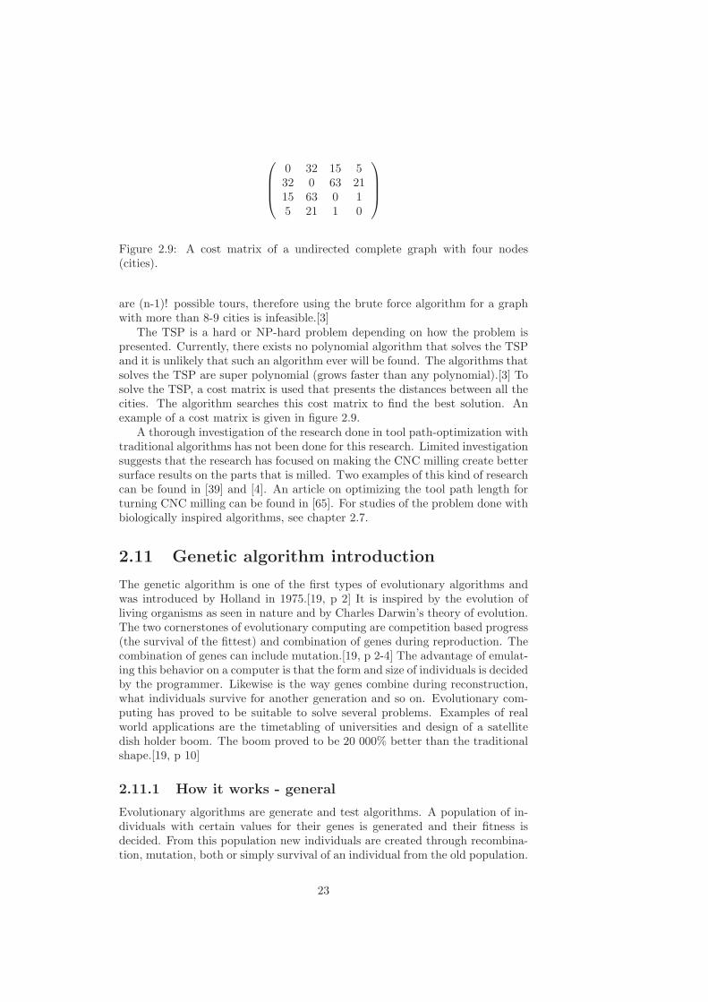
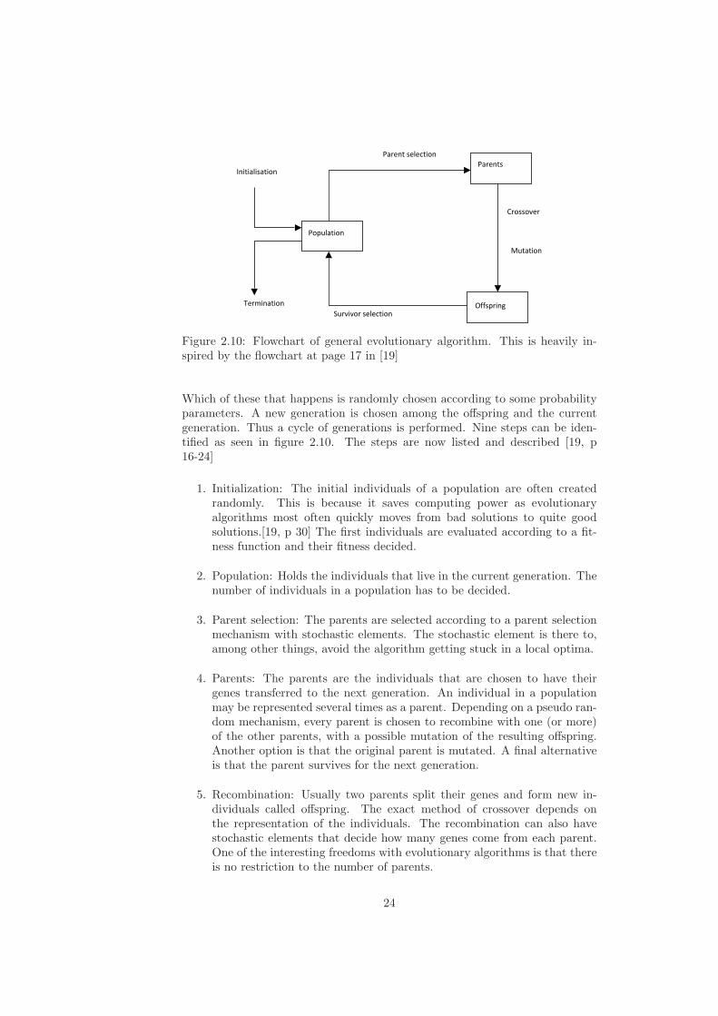
Figure 2.10: Flowchart of general evolutionary algorithm. This is heavily in-spired by the flowchart at page 17 in [19]

Which of these that happens is randomly chosen according to some probabilityparameters. A new generation is chosen among the offspring and the currentgeneration. Thus a cycle of generations is performed. Nine steps can be iden-tified as seen in figure 2.10. The steps are now listed and described [19, p16-24]

1. Initialization: The initial individuals of a population are often createdrandomly. This is because it saves computing power as evolutionaryalgorithms most often quickly moves from bad solutions to quite goodsolutions.[19, p 30] The first individuals are evaluated according to a fit-ness function and their fitness decided.

2. Population: Holds the individuals that live in the current generation. Thenumber of individuals in a population has to be decided.

3. Parent selection: The parents are selected according to a parent selectionmechanism with stochastic elements. The stochastic element is there to,among other things, avoid the algorithm getting stuck in a local optima.

4. Parents: The parents are the individuals that are chosen to have theirgenes transferred to the next generation. An individual in a populationmay be represented several times as a parent. Depending on a pseudo ran-dom mechanism, every parent is chosen to recombine with one (or more)of the other parents, with a possible mutation of the resulting offspring.Another option is that the original parent is mutated. A final alternativeis that the parent survives for the next generation.

5. Recombination: Usually two parents split their genes and form new in-dividuals called offspring. The exact method of crossover depends onthe representation of the individuals. The recombination can also havestochastic elements that decide how many genes come from each parent.One of the interesting freedoms with evolutionary algorithms is that thereis no restriction to the number of parents.

24

6. Mutation: Mutation is the random alteration of genes in a single individ-ual. As with crossover this depends on the representation of the individ-uals.

7. Offspring: These are the indivdiuals that are created from the parents.The number of offspring has to be decided. Also, the offspring must havetheir fitness evaluated.

8. Survivor selection: Among the current generation and the offspring, whoare the ones to survive for the next generation? This can be done indifferent ways, among which are: to only choose the offspring, the offspringand the best individual in the current generation or simply the fittestindividuals.

9. Termination: The termination criteria decide when the algorithm is fin-ished. This can for example be after a certain fitness has been reached.To be sure the algorithm terminates it is often smart to have a maximumnumber of generations as a safety.

As can be seen there are several steps where randomness plays a role. Thisoften makes it hard to analyze the algorithm and the results it creates withoutexperimental testing. However, the randomness is one of the strengths of theevolutionary algorithms as it makes it possible to avoid local optima.

2.12 Introduction to the Ant Colony Optimiaza-

tion algorithm

The background information presented here relies on [18]. Ant Colony Optimiza-tion (ACO) is a rather new form of optimization algorithm, being introduced inthe early nineties. It models the foraging behavior of some ant species, in partic-ular the pheromone deposition. ACOs have been successfully implemented onseveral types of optimizations problems, and specifically the Travelling SalesmanProblem.

The ants of some species deposit a substance called pheromone as they movefrom the nest to a food source. Since the pheromone evaporates, places wherethe ants use more gets more and more popular. As ants are almost blind they ori-entate themselves with the help of the concentration of pheromone deposits.[18]This was proven by Deneubourgh and Goss with the double bridge experiment.[16, 22] However, in ACOs the ants are artificial; allowing the developers to givethem features actual ants lack.

25

Chapter 3

Tools

In this chapter the tools used in this thesis is presented. Also, the type of motorsand electronics that is suitable for the robot is suggested.

3.1 Python

Python is a programming language that is free, portable, powerful and remark-ably easy and fun to use according to Mark Lutz.[37] He also stresses the lan-guage’s software quality, high developer productivity and program portability.[37,p 3-4] Another important aspect is the 3rd party libraries, two of which are thefree Numpy and Matplotlib. The 3rd party libraries make Python a very flexiblelanguage and covers topics from web programming to advanced mathematics.

3.1.1 Numpy and Matplotlib

Together with Scipy these libraries almost rivals Matlab in mathematical compu-tation. More importantly, Numpy and Matplotlib make drawing in 3D possible.This makes it possible to create a 3D simulation of the Stewart platform.

3.2 Solid Works and Solid CAM

In this thesis SolidWorks has been used as CAD software and SolidCAM hasbeen used as CAM software.[56, 55] SolidWorks has been extensively used todesign and test the design of the Stewart platform while SolidCAM has onlybeen used to verify that G-code can have a varied syntax.

There exist many different CAD and CAM software producers. [34] Solid-Works and SolidCAM was chosen simply because the University of Oslo haslicenses for the software, I had earlier experience with it and a free studentedition is available.

3.3 Stepper motors

The motor that is suggested to be used for further study of this project is a twophase hybrid stepper motor as can be seen in figure 3.1. It has high reliability,

27

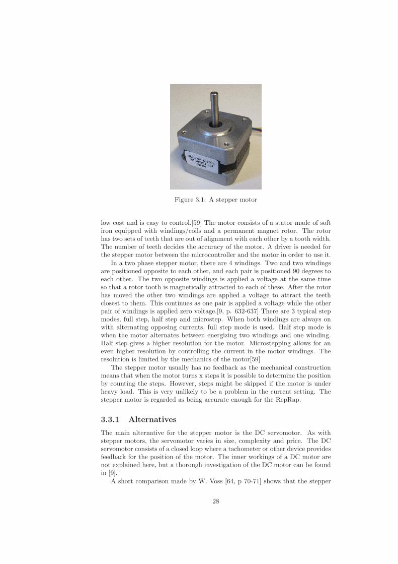
Figure 3.1: A stepper motor

low cost and is easy to control.[59] The motor consists of a stator made of softiron equipped with windings/coils and a permanent magnet rotor. The rotorhas two sets of teeth that are out of alignment with each other by a tooth width.The number of teeth decides the accuracy of the motor. A driver is needed forthe stepper motor between the microcontroller and the motor in order to use it.

In a two phase stepper motor, there are 4 windings. Two and two windingsare positioned opposite to each other, and each pair is positioned 90 degrees toeach other. The two opposite windings is applied a voltage at the same timeso that a rotor tooth is magnetically attracted to each of these. After the rotorhas moved the other two windings are applied a voltage to attract the teethclosest to them. This continues as one pair is applied a voltage while the otherpair of windings is applied zero voltage.[9, p. 632-637] There are 3 typical stepmodes, full step, half step and microstep. When both windings are always onwith alternating opposing currents, full step mode is used. Half step mode iswhen the motor alternates between energizing two windings and one winding.Half step gives a higher resolution for the motor. Microstepping allows for aneven higher resolution by controlling the current in the motor windings. Theresolution is limited by the mechanics of the motor[59]

The stepper motor usually has no feedback as the mechanical constructionmeans that when the motor turns x steps it is possible to determine the positionby counting the steps. However, steps might be skipped if the motor is underheavy load. This is very unlikely to be a problem in the current setting. Thestepper motor is regarded as being accurate enough for the RepRap.

3.3.1 Alternatives

The main alternative for the stepper motor is the DC servomotor. As withstepper motors, the servomotor varies in size, complexity and price. The DCservomotor consists of a closed loop where a tachometer or other device providesfeedback for the position of the motor. The inner workings of a DC motor arenot explained here, but a thorough investigation of the DC motor can be foundin [9].

A short comparison made by W. Voss [64, p 70-71] shows that the stepper

28

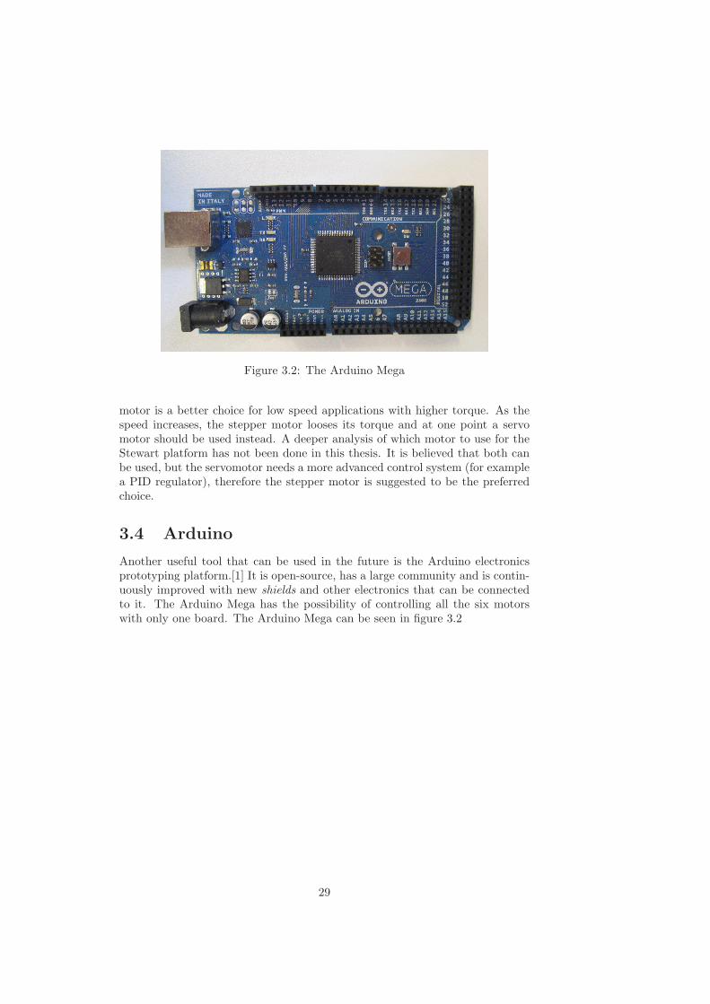
Figure 3.2: The Arduino Mega

motor is a better choice for low speed applications with higher torque. As thespeed increases, the stepper motor looses its torque and at one point a servomotor should be used instead. A deeper analysis of which motor to use for theStewart platform has not been done in this thesis. It is believed that both canbe used, but the servomotor needs a more advanced control system (for examplea PID regulator), therefore the stepper motor is suggested to be the preferredchoice.

3.4 Arduino

Another useful tool that can be used in the future is the Arduino electronicsprototyping platform.[1] It is open-source, has a large community and is contin-uously improved with new shields and other electronics that can be connectedto it. The Arduino Mega has the possibility of controlling all the six motorswith only one board. The Arduino Mega can be seen in figure 3.2

29

Chapter 4

Design

One of the most interesting aspects of this project is the physical implementationof the robot as this is where the research proves its usability. If the robot can’tbe built with the desired restrictions (see chapter 2.4 and 2.5 and especially2.5.5), then there is little use in studying the rest of the system.

As stated in the introduction, one of the goals for this thesis is to make asuggestion for a different design than the current RepRap design that preferablywould simplify the mechanical construction and allow a more diverse use byincluding CNC milling. The Stewart platform has been chosen because of itsrigidity, however the actuators can be advanced and expensive or inaccurate.One of the reasons why the design is presented in such a detail is to keep withthe idea of RepRap and make the design open-source. The designs and the ideasbehind them will be discussed. After that, a comparison with the RepRap isdone. Finally a concluding discussion sums up the experiences gathered fromdesigning a Stewart platform.

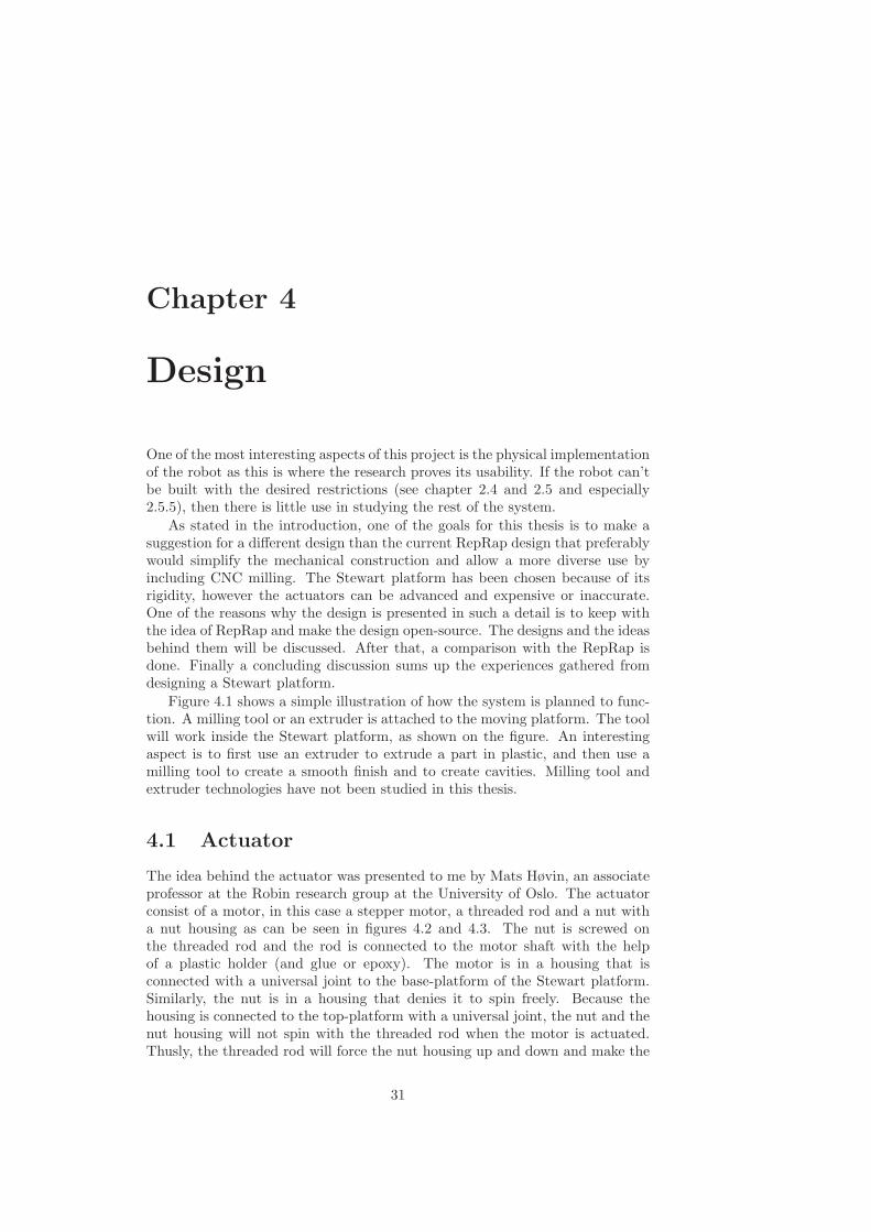
Figure 4.1 shows a simple illustration of how the system is planned to func-tion. A milling tool or an extruder is attached to the moving platform. The toolwill work inside the Stewart platform, as shown on the figure. An interestingaspect is to first use an extruder to extrude a part in plastic, and then use amilling tool to create a smooth finish and to create cavities. Milling tool andextruder technologies have not been studied in this thesis.

4.1 Actuator

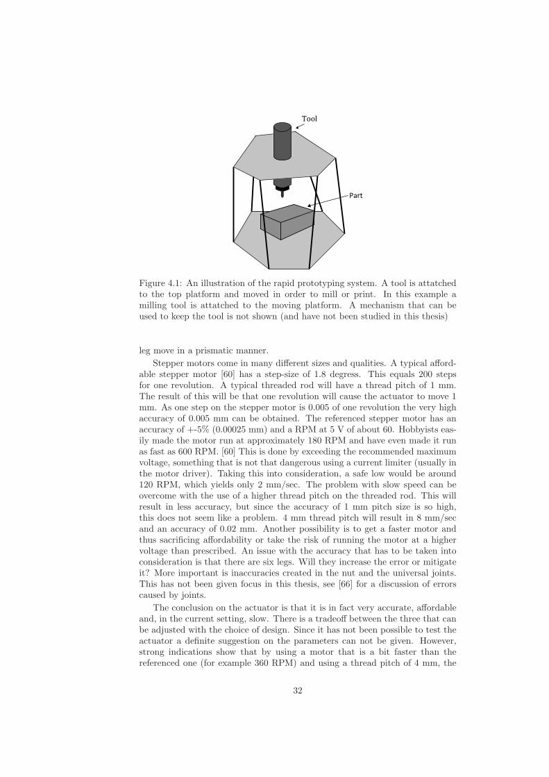
The idea behind the actuator was presented to me by Mats Høvin, an associateprofessor at the Robin research group at the University of Oslo. The actuatorconsist of a motor, in this case a stepper motor, a threaded rod and a nut witha nut housing as can be seen in figures 4.2 and 4.3. The nut is screwed onthe threaded rod and the rod is connected to the motor shaft with the helpof a plastic holder (and glue or epoxy). The motor is in a housing that isconnected with a universal joint to the base-platform of the Stewart platform.Similarly, the nut is in a housing that denies it to spin freely. Because thehousing is connected to the top-platform with a universal joint, the nut and thenut housing will not spin with the threaded rod when the motor is actuated.Thusly, the threaded rod will force the nut housing up and down and make the

31

Tool

Part

Figure 4.1: An illustration of the rapid prototyping system. A tool is attatchedto the top platform and moved in order to mill or print. In this example amilling tool is attatched to the moving platform. A mechanism that can beused to keep the tool is not shown (and have not been studied in this thesis)

leg move in a prismatic manner.

Stepper motors come in many different sizes and qualities. A typical afford-able stepper motor [60] has a step-size of 1.8 degress. This equals 200 stepsfor one revolution. A typical threaded rod will have a thread pitch of 1 mm.The result of this will be that one revolution will cause the actuator to move 1mm. As one step on the stepper motor is 0.005 of one revolution the very highaccuracy of 0.005 mm can be obtained. The referenced stepper motor has anaccuracy of +-5% (0.00025 mm) and a RPM at 5 V of about 60. Hobbyists eas-ily made the motor run at approximately 180 RPM and have even made it runas fast as 600 RPM. [60] This is done by exceeding the recommended maximumvoltage, something that is not that dangerous using a current limiter (usually inthe motor driver). Taking this into consideration, a safe low would be around120 RPM, which yields only 2 mm/sec. The problem with slow speed can beovercome with the use of a higher thread pitch on the threaded rod. This willresult in less accuracy, but since the accuracy of 1 mm pitch size is so high,this does not seem like a problem. 4 mm thread pitch will result in 8 mm/secand an accuracy of 0.02 mm. Another possibility is to get a faster motor andthus sacrificing affordability or take the risk of running the motor at a highervoltage than prescribed. An issue with the accuracy that has to be taken intoconsideration is that there are six legs. Will they increase the error or mitigateit? More important is inaccuracies created in the nut and the universal joints.This has not been given focus in this thesis, see [66] for a discussion of errorscaused by joints.

The conclusion on the actuator is that it is in fact very accurate, affordableand, in the current setting, slow. There is a tradeoff between the three that canbe adjusted with the choice of design. Since it has not been possible to test theactuator a definite suggestion on the parameters can not be given. However,strong indications show that by using a motor that is a bit faster than thereferenced one (for example 360 RPM) and using a thread pitch of 4 mm, the

32

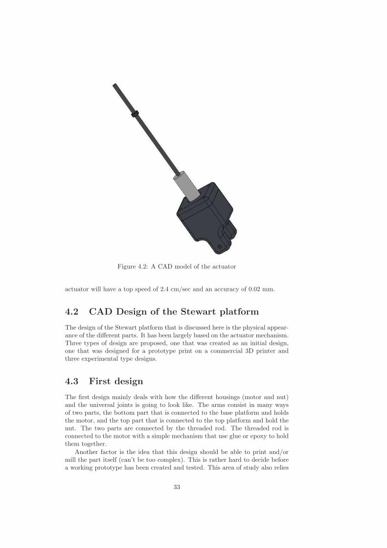
Figure 4.2: A CAD model of the actuator

actuator will have a top speed of 2.4 cm/sec and an accuracy of 0.02 mm.

4.2 CAD Design of the Stewart platform

The design of the Stewart platform that is discussed here is the physical appear-ance of the different parts. It has been largely based on the actuator mechanism.Three types of design are proposed, one that was created as an initial design,one that was designed for a prototype print on a commercial 3D printer andthree experimental type designs.

4.3 First design

The first design mainly deals with how the different housings (motor and nut)and the universal joints is going to look like. The arms consist in many waysof two parts, the bottom part that is connected to the base platform and holdsthe motor, and the top part that is connected to the top platform and hold thenut. The two parts are connected by the threaded rod. The threaded rod isconnected to the motor with a simple mechanism that use glue or epoxy to holdthem together.

Another factor is the idea that this design should be able to print and/ormill the part itself (can’t be too complex). This is rather hard to decide beforea working prototype has been created and tested. This area of study also relies

33

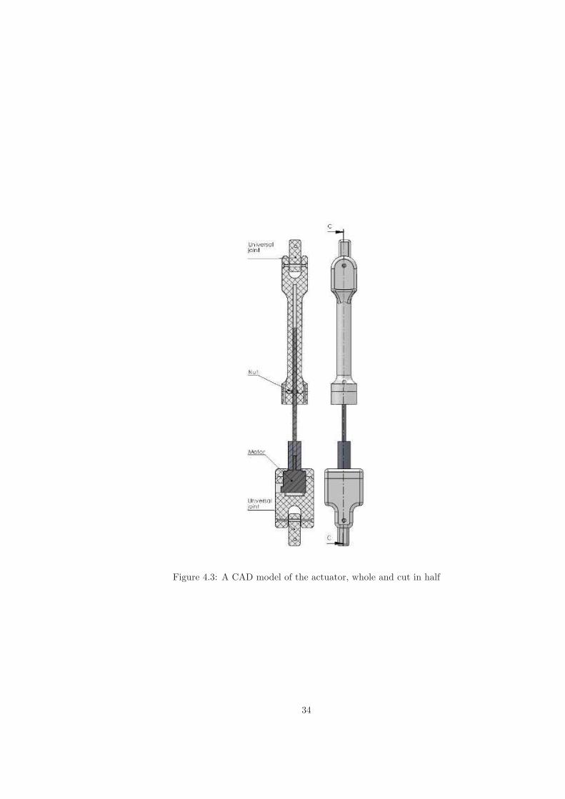
Figure 4.3: A CAD model of the actuator, whole and cut in half

34

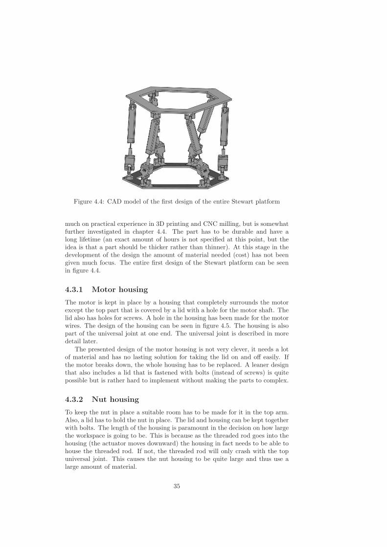
Figure 4.4: CAD model of the first design of the entire Stewart platform

much on practical experience in 3D printing and CNC milling, but is somewhatfurther investigated in chapter 4.4. The part has to be durable and have along lifetime (an exact amount of hours is not specified at this point, but theidea is that a part should be thicker rather than thinner). At this stage in thedevelopment of the design the amount of material needed (cost) has not beengiven much focus. The entire first design of the Stewart platform can be seenin figure 4.4.

4.3.1 Motor housing

The motor is kept in place by a housing that completely surrounds the motorexcept the top part that is covered by a lid with a hole for the motor shaft. Thelid also has holes for screws. A hole in the housing has been made for the motorwires. The design of the housing can be seen in figure 4.5. The housing is alsopart of the universal joint at one end. The universal joint is described in moredetail later.

The presented design of the motor housing is not very clever, it needs a lotof material and has no lasting solution for taking the lid on and off easily. Ifthe motor breaks down, the whole housing has to be replaced. A leaner designthat also includes a lid that is fastened with bolts (instead of screws) is quitepossible but is rather hard to implement without making the parts to complex.

4.3.2 Nut housing

To keep the nut in place a suitable room has to be made for it in the top arm.Also, a lid has to hold the nut in place. The lid and housing can be kept togetherwith bolts. The length of the housing is paramount in the decision on how largethe workspace is going to be. This is because as the threaded rod goes into thehousing (the actuator moves downward) the housing in fact needs to be able tohouse the threaded rod. If not, the threaded rod will only crash with the topuniversal joint. This causes the nut housing to be quite large and thus use alarge amount of material.

35

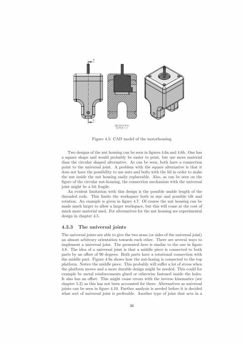
Figure 4.5: CAD model of the motorhousing

Two designs of the nut housing can be seen in figures 4.6a and 4.6b. One hasa square shape and would probably be easier to print, but use more materialthan the circular shaped alternative. As can be seen, both have a connectionpoint to the universal joint. A problem with the square alternative is that itdoes not have the possibility to use nuts and bolts with the lid in order to makethe nut inside the nut housing easily replaceable. Also, as can be seen on thefigure of the circular nut-housing, the connection mechanism with the universaljoint might be a bit fragile.

An evident limitation with this design is the possible usable length of thethreaded rods. This limits the workspace both in size and possible tilt androtation. An example is given in figure 4.7. Of course the nut housing can bemade much larger to allow a larger workspace, but this will come at the cost ofmuch more material used. For alternatives for the nut housing see experimentaldesign in chapter 4.5.

4.3.3 The universal joints

The universal joints are able to give the two arms (or sides of the universal joint)an almost arbitrary orientation towards each other. There are several ways toimplement a universal joint. The presented here is similar to the one in figure4.8. The idea of a universal joint is that a middle piece is connected to bothparts by an offset of 90 degrees. Both parts have a rotational connection withthe middle part. Figure 4.9a shows how the nut-hosing is connected to the topplatform. Notice the middle piece. This probably will suffer a lot of stress whenthe platform moves and a more durable design might be needed. This could forexample be metal reinforcements glued or otherwise fastened inside the holes.It also has an offset. This might cause errors with the inverse kinematics (seechapter 5.2) as this has not been accounted for there. Alternatives as universaljoints can be seen in figure 4.10. Further analysis is needed before it is decidedwhat sort of universal joint is preferable. Another type of joint that acts in a

36

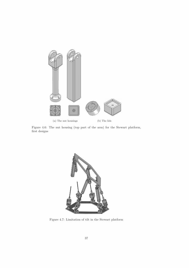
(a) The nut housings (b) The lids

Figure 4.6: The nut housing (top part of the arm) for the Stewart platform,first designs

Figure 4.7: Limitation of tilt in the Stewart platform

37

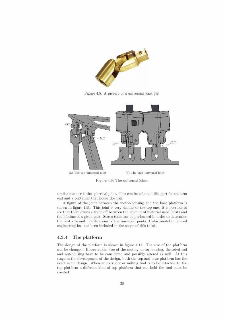
Figure 4.8: A picture of a universial joint [48]

(a) The top universal joint (b) The base universal joint

Figure 4.9: The universal joints

similar manner is the spherical joint. This consist of a ball like part for the armend and a container that house the ball.

A figure of the joint between the motor-housing and the base platform isshown in figure 4.9b. This joint is very similar to the top one. It is possible tosee that there exists a trade off between the amount of material used (cost) andthe lifetime of a given part. Stress tests can be performed in order to determinethe best size and modifications of the universal joints. Unfortunately materialengineering has not been included in the scope of this thesis.

4.3.4 The platform

The design of the platform is shown in figure 4.11. The size of the platformcan be changed. However, the size of the motor, motor-housing, threaded rodand nut-housing have to be considered and possibly altered as well. At thisstage in the development of the design, both the top and base platform has theexact same design. When an extruder or milling tool is to be attached to thetop platform a different kind of top platform that can hold the tool must becreated.

38

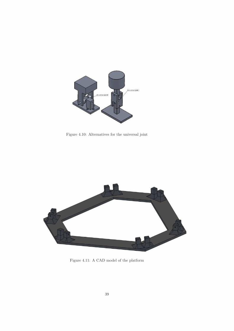
Figure 4.10: Alternatives for the universal joint

Figure 4.11: A CAD model of the platform

39

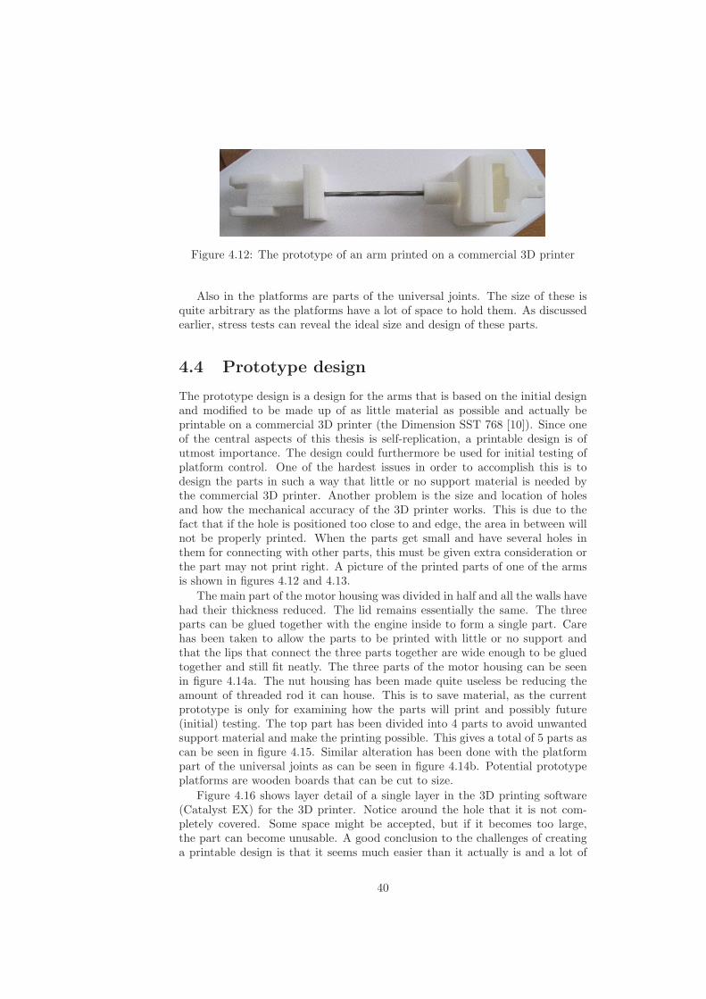
Figure 4.12: The prototype of an arm printed on a commercial 3D printer

Also in the platforms are parts of the universal joints. The size of these isquite arbitrary as the platforms have a lot of space to hold them. As discussedearlier, stress tests can reveal the ideal size and design of these parts.

4.4 Prototype design

The prototype design is a design for the arms that is based on the initial designand modified to be made up of as little material as possible and actually beprintable on a commercial 3D printer (the Dimension SST 768 [10]). Since oneof the central aspects of this thesis is self-replication, a printable design is ofutmost importance. The design could furthermore be used for initial testing ofplatform control. One of the hardest issues in order to accomplish this is todesign the parts in such a way that little or no support material is needed bythe commercial 3D printer. Another problem is the size and location of holesand how the mechanical accuracy of the 3D printer works. This is due to thefact that if the hole is positioned too close to and edge, the area in between willnot be properly printed. When the parts get small and have several holes inthem for connecting with other parts, this must be given extra consideration orthe part may not print right. A picture of the printed parts of one of the armsis shown in figures 4.12 and 4.13.

The main part of the motor housing was divided in half and all the walls havehad their thickness reduced. The lid remains essentially the same. The threeparts can be glued together with the engine inside to form a single part. Carehas been taken to allow the parts to be printed with little or no support andthat the lips that connect the three parts together are wide enough to be gluedtogether and still fit neatly. The three parts of the motor housing can be seenin figure 4.14a. The nut housing has been made quite useless be reducing theamount of threaded rod it can house. This is to save material, as the currentprototype is only for examining how the parts will print and possibly future(initial) testing. The top part has been divided into 4 parts to avoid unwantedsupport material and make the printing possible. This gives a total of 5 parts ascan be seen in figure 4.15. Similar alteration has been done with the platformpart of the universal joints as can be seen in figure 4.14b. Potential prototypeplatforms are wooden boards that can be cut to size.

Figure 4.16 shows layer detail of a single layer in the 3D printing software(Catalyst EX) for the 3D printer. Notice around the hole that it is not com-pletely covered. Some space might be accepted, but if it becomes too large,the part can become unusable. A good conclusion to the challenges of creatinga printable design is that it seems much easier than it actually is and a lot of

40

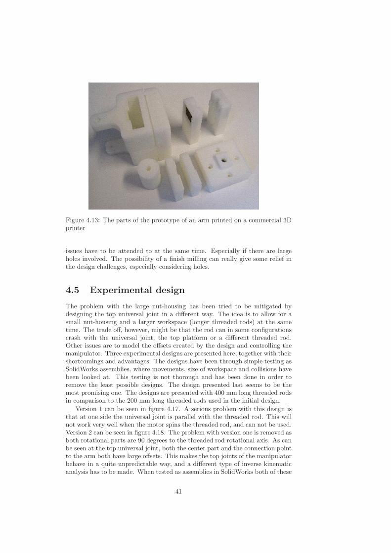
Figure 4.13: The parts of the prototype of an arm printed on a commercial 3Dprinter

issues have to be attended to at the same time. Especially if there are largeholes involved. The possibility of a finish milling can really give some relief inthe design challenges, especially considering holes.

4.5 Experimental design

The problem with the large nut-housing has been tried to be mitigated bydesigning the top universal joint in a different way. The idea is to allow for asmall nut-housing and a larger workspace (longer threaded rods) at the sametime. The trade off, however, might be that the rod can in some configurationscrash with the universal joint, the top platform or a different threaded rod.Other issues are to model the offsets created by the design and controlling themanipulator. Three experimental designs are presented here, together with theirshortcomings and advantages. The designs have been through simple testing asSolidWorks assemblies, where movements, size of workspace and collisions havebeen looked at. This testing is not thorough and has been done in order toremove the least possible designs. The design presented last seems to be themost promising one. The designs are presented with 400 mm long threaded rodsin comparison to the 200 mm long threaded rods used in the initial design.

Version 1 can be seen in figure 4.17. A serious problem with this design isthat at one side the universal joint is parallel with the threaded rod. This willnot work very well when the motor spins the threaded rod, and can not be used.Version 2 can be seen in figure 4.18. The problem with version one is removed asboth rotational parts are 90 degrees to the threaded rod rotational axis. As canbe seen at the top universal joint, both the center part and the connection pointto the arm both have large offsets. This makes the top joints of the manipulatorbehave in a quite unpredictable way, and a different type of inverse kinematicanalysis has to be made. When tested as assemblies in SolidWorks both of these

41

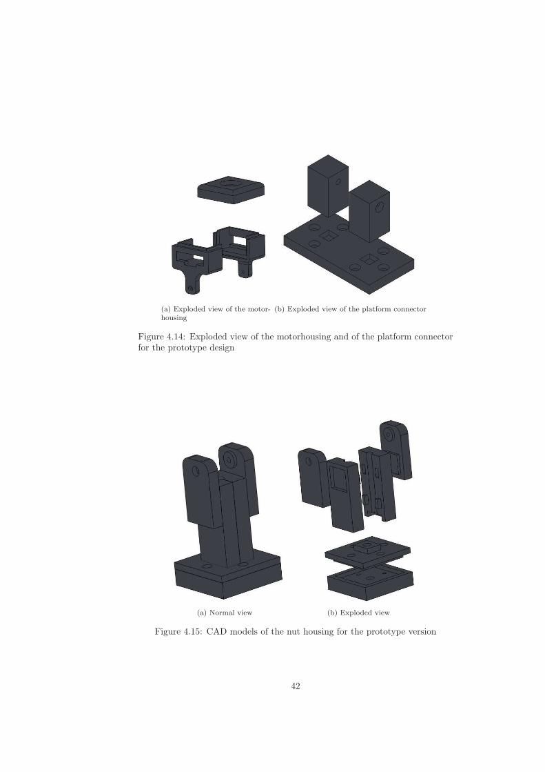
(a) Exploded view of the motor-housing

(b) Exploded view of the platform connector

Figure 4.14: Exploded view of the motorhousing and of the platform connectorfor the prototype design

(a) Normal view (b) Exploded view

Figure 4.15: CAD models of the nut housing for the prototype version

42

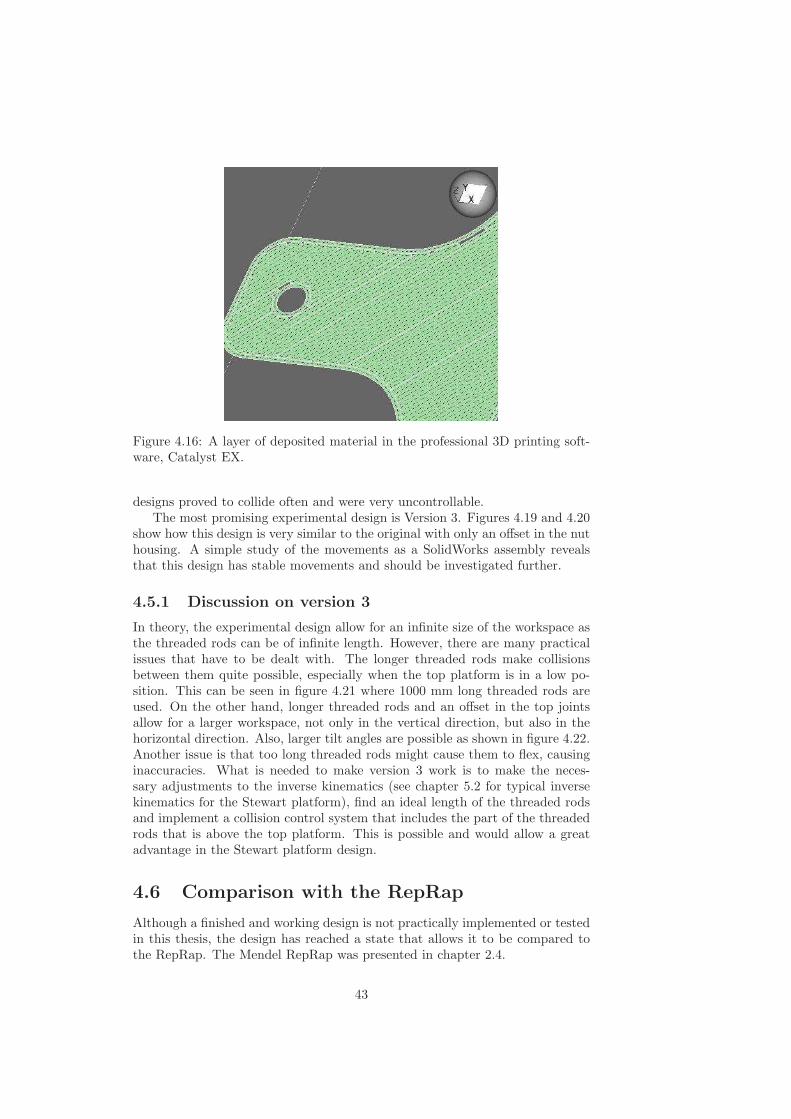
Figure 4.16: A layer of deposited material in the professional 3D printing soft-ware, Catalyst EX.

designs proved to collide often and were very uncontrollable.The most promising experimental design is Version 3. Figures 4.19 and 4.20

show how this design is very similar to the original with only an offset in the nuthousing. A simple study of the movements as a SolidWorks assembly revealsthat this design has stable movements and should be investigated further.

4.5.1 Discussion on version 3

In theory, the experimental design allow for an infinite size of the workspace asthe threaded rods can be of infinite length. However, there are many practicalissues that have to be dealt with. The longer threaded rods make collisionsbetween them quite possible, especially when the top platform is in a low po-sition. This can be seen in figure 4.21 where 1000 mm long threaded rods areused. On the other hand, longer threaded rods and an offset in the top jointsallow for a larger workspace, not only in the vertical direction, but also in thehorizontal direction. Also, larger tilt angles are possible as shown in figure 4.22.Another issue is that too long threaded rods might cause them to flex, causinginaccuracies. What is needed to make version 3 work is to make the neces-sary adjustments to the inverse kinematics (see chapter 5.2 for typical inversekinematics for the Stewart platform), find an ideal length of the threaded rodsand implement a collision control system that includes the part of the threadedrods that is above the top platform. This is possible and would allow a greatadvantage in the Stewart platform design.

4.6 Comparison with the RepRap

Although a finished and working design is not practically implemented or testedin this thesis, the design has reached a state that allows it to be compared tothe RepRap. The Mendel RepRap was presented in chapter 2.4.

43

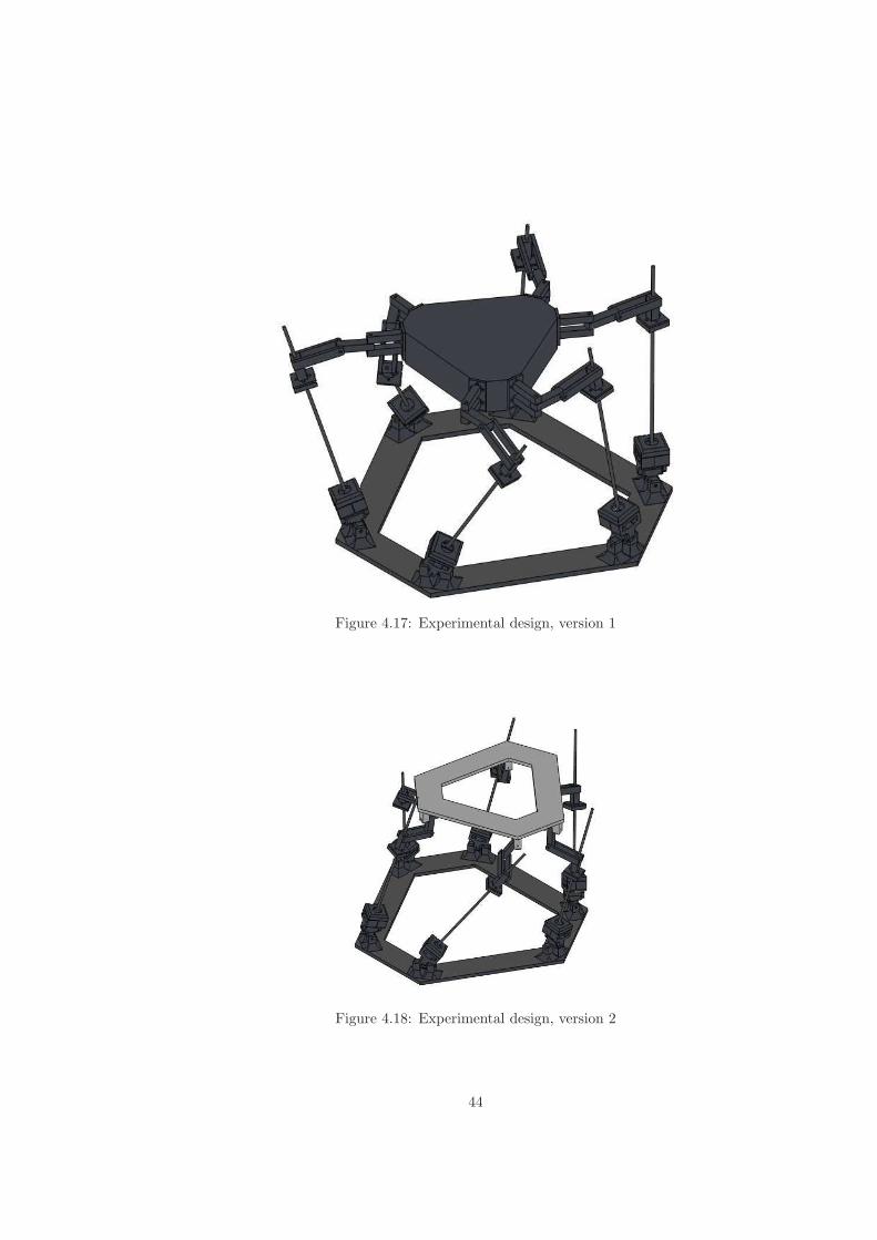
Figure 4.17: Experimental design, version 1

Figure 4.18: Experimental design, version 2

44

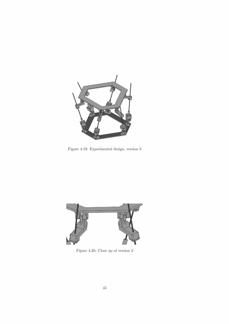
Figure 4.19: Experimental design, version 3

Figure 4.20: Close up of version 3

45

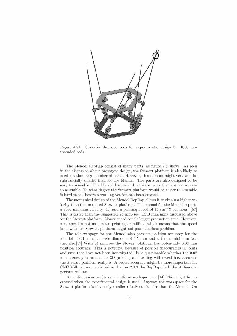
Figure 4.21: Crash in threaded rods for experimental design 3. 1000 mmthreaded rods.

The Mendel RepRap consist of many parts, as figure 2.5 shows. As seenin the discussion about prototype design, the Stewart platform is also likely toneed a rather large number of parts. However, this number might very well besubstantially smaller than for the Mendel. The parts are also designed to beeasy to assemble. The Mendel has several intricate parts that are not so easyto assemble. To what degree the Stewart platform would be easier to assembleis hard to tell before a working version has been created.

The mechanical design of the Mendel RepRap allows it to obtain a higher ve-locity than the presented Stewart platform. The manual for the Mendel reportsa 3000 mm/min velocity [40] and a printing speed of 15 cm**3 per hour. [57]This is faster than the suggested 24 mm/sec (1440 mm/min) discussed abovefor the Stewart platform. Slower speed equals longer production time. However,max speed is not used when printing or milling, which means that the speedissue with the Stewart platform might not pose a serious problem.

The wiki-webpage for the Mendel also presents position accuracy for theMendel of 0.1 mm, a nozzle diameter of 0.5 mm and a 2 mm minimum fea-ture size.[57] With 24 mm/sec the Stewart platform has potentially 0.02 mmposition accuracy. This is potential because of possible inaccuracies in jointsand nuts that have not been investigated. It is questionable whether the 0.02mm accuracy is needed for 3D printing and testing will reveal how accuratethe Stewart platform really is. A better accuracy might be more important forCNC Milling. As mentioned in chapter 2.4.3 the RepRaps lack the stiffness toperform milling.

For a discussion on Stewart platform workspace see.[14] This might be in-creased when the experimental design is used. Anyway, the workspace for theStewart platform is obviously smaller relative to its size than the Mendel. On

46

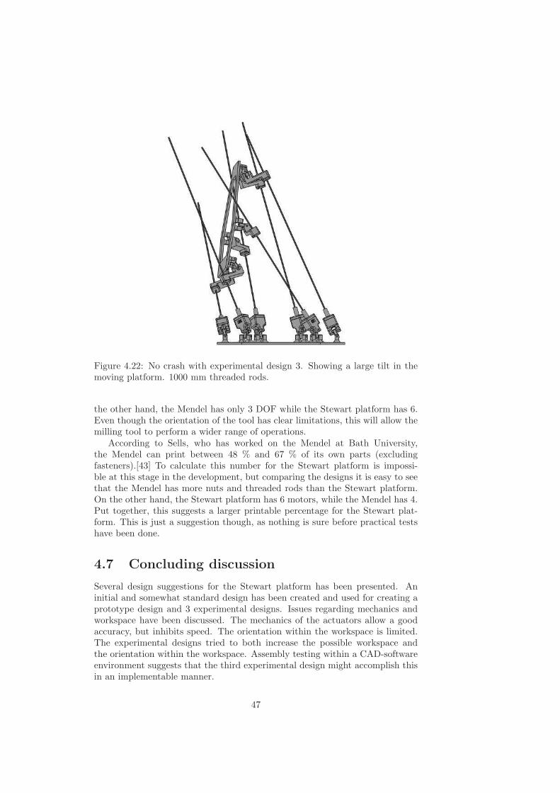
Figure 4.22: No crash with experimental design 3. Showing a large tilt in themoving platform. 1000 mm threaded rods.

the other hand, the Mendel has only 3 DOF while the Stewart platform has 6.Even though the orientation of the tool has clear limitations, this will allow themilling tool to perform a wider range of operations.

According to Sells, who has worked on the Mendel at Bath University,the Mendel can print between 48 % and 67 % of its own parts (excludingfasteners).[43] To calculate this number for the Stewart platform is impossi-ble at this stage in the development, but comparing the designs it is easy to seethat the Mendel has more nuts and threaded rods than the Stewart platform.On the other hand, the Stewart platform has 6 motors, while the Mendel has 4.Put together, this suggests a larger printable percentage for the Stewart plat-form. This is just a suggestion though, as nothing is sure before practical testshave been done.

4.7 Concluding discussion

Several design suggestions for the Stewart platform has been presented. Aninitial and somewhat standard design has been created and used for creating aprototype design and 3 experimental designs. Issues regarding mechanics andworkspace have been discussed. The mechanics of the actuators allow a goodaccuracy, but inhibits speed. The orientation within the workspace is limited.The experimental designs tried to both increase the possible workspace andthe orientation within the workspace. Assembly testing within a CAD-softwareenvironment suggests that the third experimental design might accomplish thisin an implementable manner.

47

A simple prototype of a single arm was printed on a commercial 3D printerin order to suggest that the Stewart platform in the future will be capable tocreate the plastic parts it is made of. As self-replication is one of the centralaspects in this thesis, a printable design is very important. The succesful print ofthe parts (figures 4.12 and 4.13) proved that this is very likely to be true. Thenext step in this regard could be to expand on the current prototype designto become more applicable as parts for a Stewart platform, in other wordsto increase the length of the nut housing, to put together and test an entireStewart platform according to the prototype design or to use the experiencefrom creating a prototype design to perform the same analysis and changes tothe third experimental design.

The comparison with the RepRap Mendel suggests that the Stewart platformcan in fact be an alternative to the current RepRap design. It is importantto stress the can aspect of this possibility. Much more practical developmentand testing have to be performed before the can turns into a is . The abovediscussion has also showed that true 3D milling with a Stewart platform canbe very difficult because even though it has 6 DOF, not all orientations aremechanically reachable. However, 2.5 D milling seems very possible and alsoto allow the milling tool some tilt. A solution to this problem has been doneby PKMTricept [50] as can be seen in figure 2.4. Here, instead of a Stewartplatform (or a hexapod), a tripod is used for 3 DOF positioning. The platformhangs from a structure and at the movable platform a small and rigid serialmanipulator (robot arm) is positioned. Depending on the model, this has 2 - 3DOF and allows a quite arbitrary orientation of the milling tool. This solutionis a professional and industrial one and could not be easily implemented withinthe RepRap concept. Maybe if the manipulator is attached to the underside ofa desk, a solution can be reached. However, these are just speculations.

This chapter shows more than anything that there are many areas to explorewith the Stewart platform and research possibilities are abundant and varied.The CAD software was very useful for testing the motion of the Stewart platformin assembly mode where the different parts can be connected together with thehelp of mates and the actual movements of the manipulator can be studied.

One aspect that has not been studied is how the actual milling tool andextruder is to be attached to the moving platform. This is a practical problemthat relies much on the kind of milling tool and extruder and should not behard to overcome. A solution could be to have some kind of holder on themoving platform, allowing the milling tool and the extruder to be changedaccording to what procedure the robot is going to perform next. Another aspectthat remanins untouched is the issue of rigidity. Practical testing or advanceddynamical testing is needed to verify whether the presented designs are rigidenough to mill.

48

Chapter 5

Simulator

A simulator was developed for the Stewart platform in order to be able to analyzethe movements and actions of the platform and to further study it in the future.The simulator was written using the python language (see chapter 3.1) anddeveloped with inverse kinematics that describes the position and orientationof the platforms and legs when the position and orientation of the end-effectoris known. As mentioned earlier this is quite simple for a parallel manipulator,while the other way around, deciding where the end-effector is given the lengthof the legs, is mathematically complex. When working with 3D printing andCNC milling, the location and orientation of the end-effector is always given,thus this does not pose a serious problem.

5.1 Uses for the simulator

There are several possible uses for a simulator. However, the current simula-tor needs some improvements to allow all the listed functions to be possible.Circular interpolation is for example important to have implemented.

• Testing code to make sure no collision happens.

• Testing code to make sure no legs are to move beyond their limitations

• Make sure the tool path is correct

• Examine how many degrees a motor has spun

• Examine the length of the tool path

• Examine execution time

• Examine the size of the workspace

The functions that have been implemented are to make sure no collisionhappens, make sure no legs move beyond their limitations and make sure thetool path is correct. To examine the workspace is reportedly a complex matterand this problem has not been studied. The rest of the functions that have notbeen implemented are discussed in chapter 5.4.2.

49

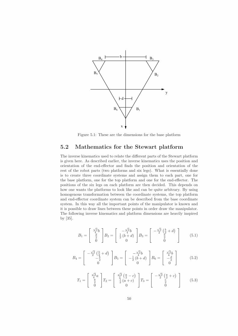
y

x

B3

B2

B1B6

B5

B4b

d

Figure 5.1: These are the dimensions for the base platform

5.2 Mathematics for the Stewart platform

The inverse kinematics used to relate the different parts of the Stewart platformis given here. As described earlier, the inverse kinematics uses the position andorientation of the end-effector and finds the position and orientation of therest of the robot parts (two platforms and six legs). What is essentially doneis to create three coordinate systems and assign them to each part, one forthe base platform, one for the top platform and one for the end-effector. Thepositions of the six legs on each platform are then decided. This depends onhow one wants the platforms to look like and can be quite arbitrary. By usinghomogenous transformation between the coordinate systems, the top platformand end-effector coordinate system can be described from the base coordinatesystem. In this way all the important points of the manipulator is known andit is possible to draw lines between these points in order draw the manipulator.The following inverse kinematics and platform dimensions are heavily inspiredby [35].

B1 =

√

3

4b

d2

0

B2 =

−

√

3

4b

1

2(b+ d)0

B3 =

−

√

3

2

(

b2+ d

)

b2

0

(5.1)

B4 =

−

√

3

2

(

b2+ d

)

−b2

0

B5 =

−

√

3

4b

−1

2(b+ d)0

B6 =

√

3

4b

−d2

0

(5.2)

T1 =

√

3

4a

a2

0

T2 =

√

3

2

(

a2− c

)

1

2(a+ c)0

T3 =

−

√

3

2

(

a2+ c

)

c2

0

(5.3)

50

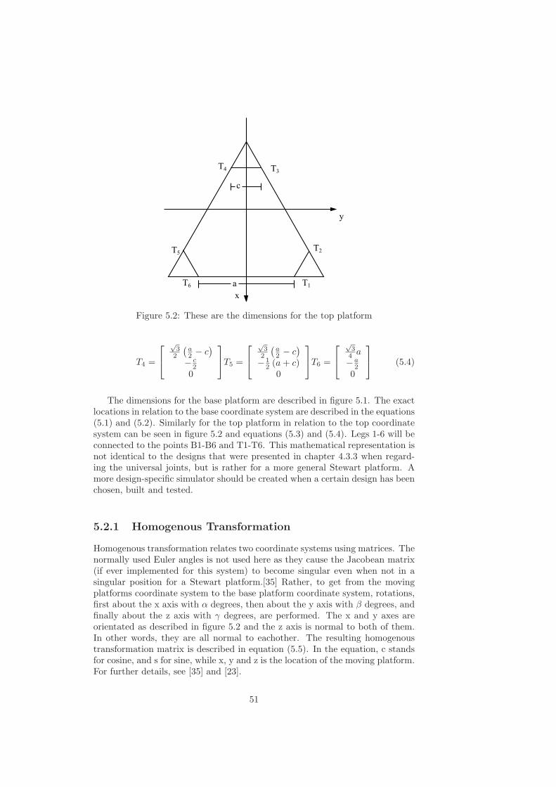
y

x

T1

T2

T3T4

T5

T6 a

c

Figure 5.2: These are the dimensions for the top platform

T4 =

√

3

2

(

a2− c

)

−c2

0

T5 =

√

3

2

(

a2− c

)

−1

2(a+ c)0

T6 =

√

3

4a

−a2

0

(5.4)

The dimensions for the base platform are described in figure 5.1. The exactlocations in relation to the base coordinate system are described in the equations(5.1) and (5.2). Similarly for the top platform in relation to the top coordinatesystem can be seen in figure 5.2 and equations (5.3) and (5.4). Legs 1-6 will beconnected to the points B1-B6 and T1-T6. This mathematical representation isnot identical to the designs that were presented in chapter 4.3.3 when regard-ing the universal joints, but is rather for a more general Stewart platform. Amore design-specific simulator should be created when a certain design has beenchosen, built and tested.

5.2.1 Homogenous Transformation

Homogenous transformation relates two coordinate systems using matrices. Thenormally used Euler angles is not used here as they cause the Jacobean matrix(if ever implemented for this system) to become singular even when not in asingular position for a Stewart platform.[35] Rather, to get from the movingplatforms coordinate system to the base platform coordinate system, rotations,first about the x axis with α degrees, then about the y axis with β degrees, andfinally about the z axis with γ degrees, are performed. The x and y axes areorientated as described in figure 5.2 and the z axis is normal to both of them.In other words, they are all normal to eachother. The resulting homogenoustransformation matrix is described in equation (5.5). In the equation, c standsfor cosine, and s for sine, while x, y and z is the location of the moving platform.For further details, see [35] and [23].

51

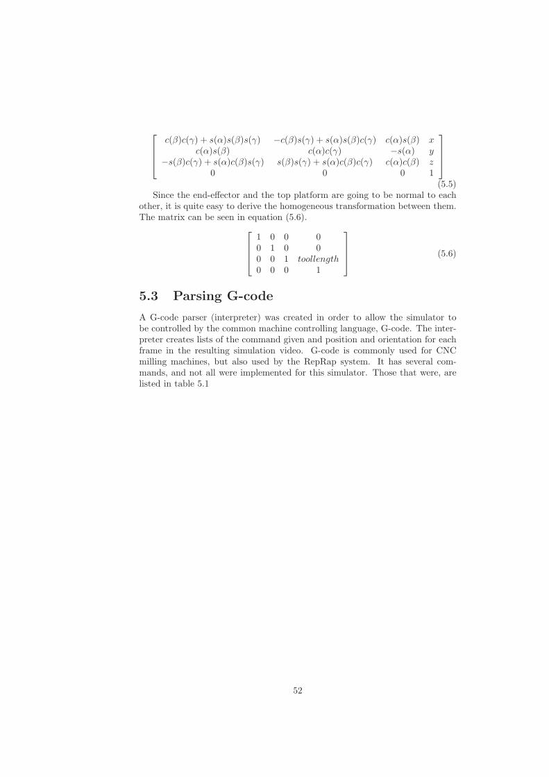
c(β)c(γ) + s(α)s(β)s(γ) −c(β)s(γ) + s(α)s(β)c(γ) c(α)s(β) xc(α)s(β) c(α)c(γ) −s(α) y

−s(β)c(γ) + s(α)c(β)s(γ) s(β)s(γ) + s(α)c(β)c(γ) c(α)c(β) z0 0 0 1

(5.5)Since the end-effector and the top platform are going to be normal to each

other, it is quite easy to derive the homogeneous transformation between them.The matrix can be seen in equation (5.6).

1 0 0 00 1 0 00 0 1 toollength0 0 0 1

(5.6)

5.3 Parsing G-code

A G-code parser (interpreter) was created in order to allow the simulator tobe controlled by the common machine controlling language, G-code. The inter-preter creates lists of the command given and position and orientation for eachframe in the resulting simulation video. G-code is commonly used for CNCmilling machines, but also used by the RepRap system. It has several com-mands, and not all were implemented for this simulator. Those that were, arelisted in table 5.1

52

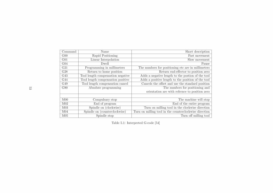
Command Name Short descriptionG00 Rapid Positioning Fast movementG01 Linear Interpolation Slow movementG04 Dwell PauseG21 Programming in millimeters The numbers for positioning etc are in millimetersG28 Return to home position Return end-effector to position zeroG43 Tool length compensation negative Adds a negative length to the postion of the toolG44 Tool length compensation positive Adds a positive length to the position of the toolG49 Tool length compensation cancel Cancels the offset and use the standard positionG90 Absolute programming The numbers for positioning and

orientation are with refernce to position zero

M00 Compulsary stop The machine will stopM02 End of program End of the entire programM03 Spindle on (clockwise) Turn on milling tool in the clockwise directionM04 Spindle on (counterclockwise) Turn on milling tool in the counterclockwise directionM05 Spindle stop Turn off milling tool

Table 5.1: Interpreted G-code [54]

53

Notable omissions are programming in inches, local coordinate system, in-cremental programming and circular interpolation. Also, subroutines have notbeen implemented. A complete G-code parser that would incorporate all thedifferent variations of G-code is very time consuming and hard to create. How-ever the most important commands for this simulator is the rapid and linearpositioning (location and orientation) to be able to locate the end-effector, andfrom that draw the entire Stewart platform. In G-code X, Y and Z sets theposition, A, B and C the orientation, H is positioned in front of tool lengthoffsets and P, X and U is used in front of the value for dwell time.

The syntax or format of different G-code files has been found to be quitedifferent. There is for example a difference in the use of lined numbers. Theparser made for this thesis reads only G-code with numbered lines according tothe “Nx standard” (for example N10, N20, N30 etc). This is how the syntaxof G-code has been presented in a classic CNC machining book.[54] Becauseof these variations in syntax, some G-code files can not be read at all by theparser.

5.4 Results

The simulator has been tested in order to verify it capabilities. In order to beable to perform most of the functions listed in chapter 5.1, the simulator shouldbe capable of

• Determining the current command

• Determining the specified speed

• Determining the calculated absolute speed of the end-effector

• Determining whether the tool is on or off.

• Determining how much the tool offset is specified to. This is necessary formilling where the bits might have different sizes.

• Determining the position of the tip of the end-effector

• Determining the orientation of the end-effector

• Determining the absolute speed for each of the six legs

• Create a moving image of the Stewart platform

• Show the end-effector path

The size of the platform in the simulation have been specified to be the sameas the ones presented in chapter 7.1 about the design. The value for a and b is400 mm and c and d are 250 mm. The tip of the end-effector is located 150 mmaway from the top platform. The maximum speed of the platform is discussedin chapter 4.1. For the simulator the speed is sat to 30 mm/s for fast movements(when the tool is turned off) and 15 mm/s for slow movements (when the toolis turned on). The speed for slow movements can not in a milling applicationbe decided like this, but have to be adjusted according to the material to bemilled, spindle speed, the type of bit used by the milling tool and so on. The

54

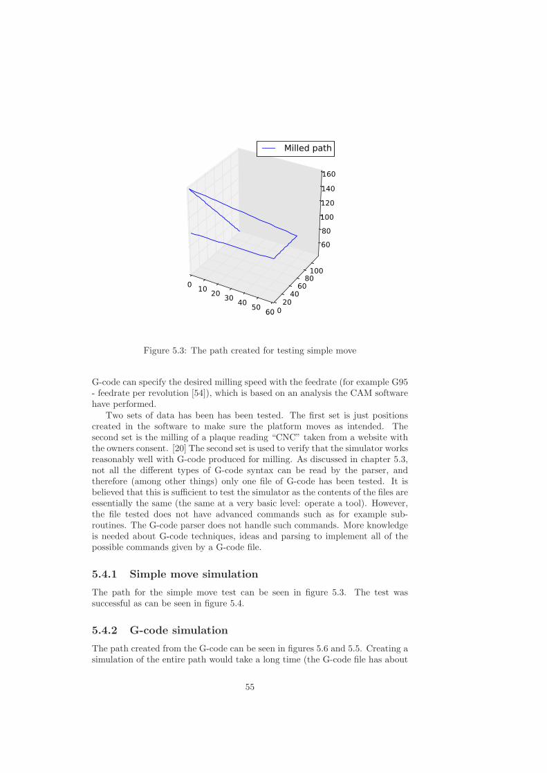
010

2030

4050

60 020406080100

60

80

100

120

140

160

Milled path

010

2030

4050

60 020406080100

60

80

100

120

140

160

Milled path

Figure 5.3: The path created for testing simple move

G-code can specify the desired milling speed with the feedrate (for example G95- feedrate per revolution [54]), which is based on an analysis the CAM softwarehave performed.

Two sets of data has been has been tested. The first set is just positionscreated in the software to make sure the platform moves as intended. Thesecond set is the milling of a plaque reading “CNC” taken from a website withthe owners consent. [20] The second set is used to verify that the simulator worksreasonably well with G-code produced for milling. As discussed in chapter 5.3,not all the different types of G-code syntax can be read by the parser, andtherefore (among other things) only one file of G-code has been tested. It isbelieved that this is sufficient to test the simulator as the contents of the files areessentially the same (the same at a very basic level: operate a tool). However,the file tested does not have advanced commands such as for example sub-routines. The G-code parser does not handle such commands. More knowledgeis needed about G-code techniques, ideas and parsing to implement all of thepossible commands given by a G-code file.

5.4.1 Simple move simulation

The path for the simple move test can be seen in figure 5.3. The test wassuccessful as can be seen in figure 5.4.

5.4.2 G-code simulation

The path created from the G-code can be seen in figures 5.6 and 5.5. Creating asimulation of the entire path would take a long time (the G-code file has about

55

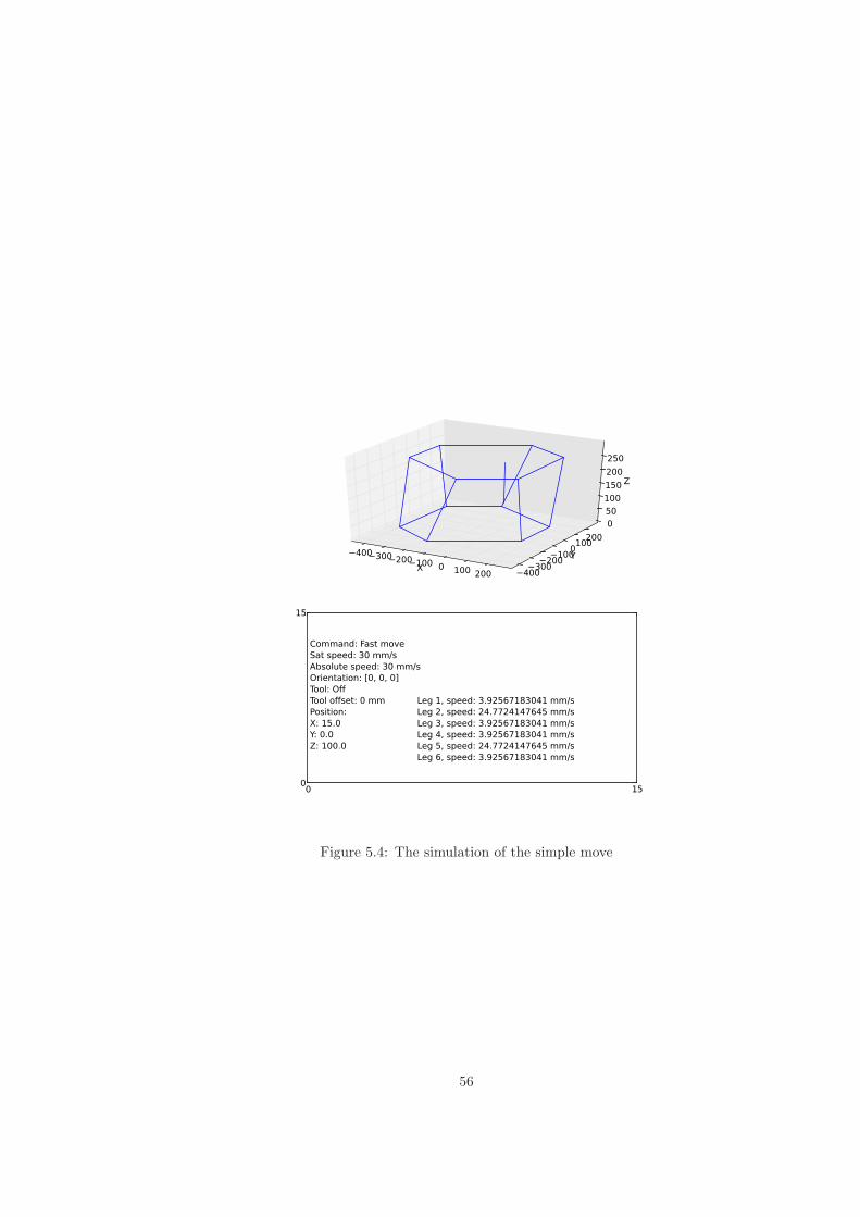
X

−400−300−200−100 0 100 200

Y

−400−300

−200−100

0100

200

Z

0

50

100

150

200

250

X

−400−300−200−100 0 100 200

Y

−400−300

−200−100

0100

200

Z

0

50

100

150

200

250

0 150

15

Command: Fast moveSat speed: 30 mm/sAbsolute speed: 30 mm/sOrientation: [0, 0, 0]Tool: OffTool offset: 0 mmPosition: X: 15.0Y: 0.0Z: 100.0

Leg 1, speed: 3.92567183041 mm/sLeg 2, speed: 24.7724147645 mm/sLeg 3, speed: 3.92567183041 mm/sLeg 4, speed: 3.92567183041 mm/sLeg 5, speed: 24.7724147645 mm/sLeg 6, speed: 3.92567183041 mm/s

Figure 5.4: The simulation of the simple move

56

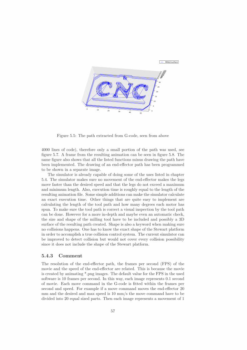
0 10 20 30 40 50

0

5

10

15

20

25

30

979899100101102103104105

Milled surface

0 10 20 30 40 50

0

5

10

15

20

25

30

979899100101102103104105

Milled surface

Figure 5.5: The path extracted from G-code, seen from above

4000 lines of code), therefore only a small portion of the path was used, seefigure 5.7. A frame from the resulting animation can be seen in figure 5.8. Thesame figure also shows that all the listed functions minus drawing the path havebeen implemented. The drawing of an end-effector path has been programmedto be shown in a separate image.

The simulator is already capable of doing some of the uses listed in chapter5.4. The simulator makes sure no movement of the end-effector makes the legsmove faster than the desired speed and that the legs do not exceed a maximumand minimum length. Also, execution time is roughly equal to the length of theresulting animation file. Some simple additions can make the simulator calculatean exact execution time. Other things that are quite easy to implement arecalculating the length of the tool path and how many degrees each motor hasspun. To make sure the tool path is correct a visual inspection by the tool pathcan be done. However for a more in-depth and maybe even an automatic check,the size and shape of the milling tool have to be included and possibly a 3Dsurface of the resulting path created. Shape is also a keyword when making sureno collisions happens. One has to know the exact shape of the Stewart platformin order to accomplish a true collision control system. The current simulator canbe improved to detect collision but would not cover every collision possibilitysince it does not include the shape of the Stewart platform.

5.4.3 Comment

The resolution of the end-effector path, the frames per second (FPS) of themovie and the speed of the end-effector are related. This is because the movieis created by animating *.png images. The default value for the FPS in the usedsoftware is 10 frames per second. In this way, each image represents 0.1 secondof movie. Each move command in the G-code is fitted within the frames persecond and speed. For example if a move command moves the end-effector 20mm and the desired and max speed is 10 mm/s the move command have to bedivided into 20 equal sized parts. Then each image represents a movement of 1

57

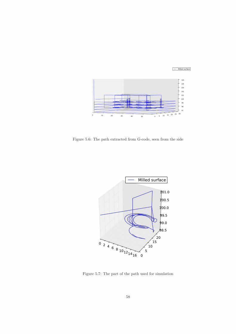
0 10 20 30 40 50 0 5 10 15 20 25 30

97

98

99

100

101

102

103

104

105

Milled surface

0 10 20 30 40 50 0 5 10 15 20 25 30

97

98

99

100

101

102

103

104

105

Milled surface

Figure 5.6: The path extracted from G-code, seen from the side

0 2 4 6 8 10121416 0510

1520

98.5

99.0

99.5

100.0

100.5

101.0

Milled surface

0 2 4 6 8 10121416 0510

1520

98.5

99.0

99.5

100.0

100.5

101.0

Milled surface

Figure 5.7: The part of the path used for simulation

58

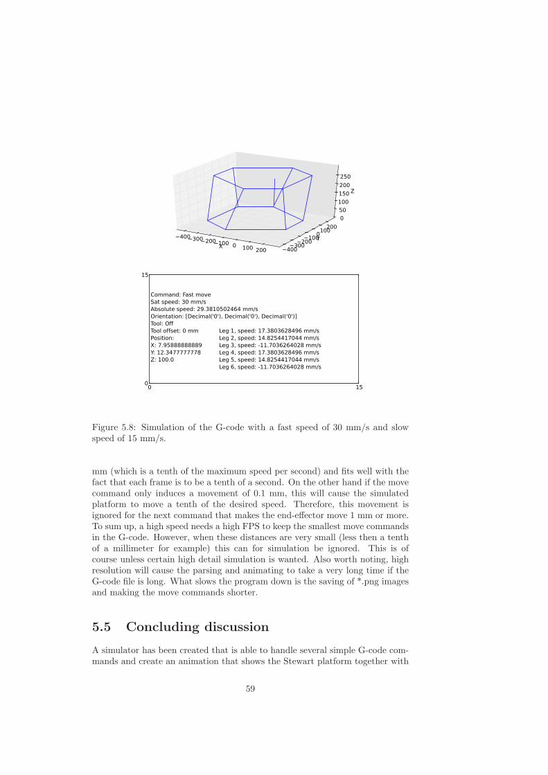
X

−400−300−200−100 0 100 200

Y

−400−300

−200−100

0100

200

Z

0

50

100

150

200

250

X

−400−300−200−100 0 100 200

Y

−400−300

−200−100

0100

200

Z

0

50

100

150

200

250

0 150

15

Command: Fast moveSat speed: 30 mm/sAbsolute speed: 29.3810502464 mm/sOrientation: [Decimal('0'), Decimal('0'), Decimal('0')]Tool: OffTool offset: 0 mmPosition: X: 7.95888888889Y: 12.3477777778Z: 100.0

Leg 1, speed: 17.3803628496 mm/sLeg 2, speed: 14.8254417044 mm/sLeg 3, speed: -11.7036264028 mm/sLeg 4, speed: 17.3803628496 mm/sLeg 5, speed: 14.8254417044 mm/sLeg 6, speed: -11.7036264028 mm/s

Figure 5.8: Simulation of the G-code with a fast speed of 30 mm/s and slowspeed of 15 mm/s.

mm (which is a tenth of the maximum speed per second) and fits well with thefact that each frame is to be a tenth of a second. On the other hand if the movecommand only induces a movement of 0.1 mm, this will cause the simulatedplatform to move a tenth of the desired speed. Therefore, this movement isignored for the next command that makes the end-effector move 1 mm or more.To sum up, a high speed needs a high FPS to keep the smallest move commandsin the G-code. However, when these distances are very small (less then a tenthof a millimeter for example) this can for simulation be ignored. This is ofcourse unless certain high detail simulation is wanted. Also worth noting, highresolution will cause the parsing and animating to take a very long time if theG-code file is long. What slows the program down is the saving of *.png imagesand making the move commands shorter.

5.5 Concluding discussion

A simulator has been created that is able to handle several simple G-code com-mands and create an animation that shows the Stewart platform together with

59

details of position, orientation, speed, tool offset, tool state (on/off) and currentcommand. There are still several commands that have not been implemented.Whether the simulator needs to be able to handle all the commands in the G-code syntax depends on the application the simulator is used for. Another issueis that there exist no standard G-code. A command might mean different thingswhen written for different applications. The simulator is capable of being usedas an analyzing tool to discover collisions, to make sure the tool path and thelength of the legs is correct and to examine speeds and time of operation. Thetwo first have to be done manually, by studying the animation and a figure ofthe tool path. Other capabilities such as calculating the length of the tool pathand calculating the number of degrees the motors have spun is not implemented,but can quite easily be so. A more sophisticated and accurate collision analysisand time calculation is possible. Workspace analysis is also possible, but hasnot been studied in this thesis due to its complexity. The study and creation ofa simulator has successfully deepened my understanding not only of the Stewartplatform, but also of the G-code language.

60

Chapter 6

Biologically Inspired

Path-Optimization

The goal for this chapter is to present two possible solutions to improve thepath of the end-effector, make a short comparison and discuss the applicabilityof the algorithms and the current approach to path-optimization (shortening thepaths where the tool is inactive). The two algorithms presented are the geneticalgorithm and the ant colony optimization algorithm. One of the reasons fordoing this study is that some papers have looked at the possibility to do thesimilar things with positive results (see chapter 2.7 for details). Another, moreobvious reason is that by optimizing the tool path, machining time can bereduced. The idea is to find shorter paths between the active paths, in otherwords, to find shorter inactive paths. I hope to take the research a step furtherby including actual G-code used for CNC-milling in the equation. This quicklymakes things much more complicated as G-code does not have a standard andthere are many practical problems that can occur. As discussed later, someof these practical problems have to some extent been ignored because they areoutside the scope of this thesis.

6.1 Research method

Eiben and Smith discuss how to work with evolutionary algorithms and how tomeasure their performance.[19, p241-258] Working with evolutionary algorithms(and ant colony optimization) most often takes an experimental approach. Theuse of randomness in the algorithms demands this as it will not behave the sameevery time. An experimental approach is when the algorithm is implementedand run with specified parameters on a set of test data and results are recordedand analyzed. This is repeated for different parameters or perhaps different testdata and the different results are compared with each other in order to get animpression of the algorithm’s performance.

The first distinction they make is between design (one-off) models and repet-itive problems. The path-optimization problem is a kind of hybrid. It is arepetitive problem in that it will be done several times. For repetitive problemsall runs of the algorithm need to present a solution that is good enough. Thisis the opposite for design problems, where one really good solution is needed.

61

However, since the amount of time in this situation is not as important as for atypical repetitive problem, the algorithm can have an adequate speed or be runseveral times in order to locate a near optimal solution. If the solution is notgood enough, the user can decide to use the original path or run the algorithmagain. This do not mean that the algorithm can behave like a design algorithm,but has some flexibility when it comes to producing good enough results excep-tionally fast versus producing optimal results. The input data is different fromrun to run so the algorithm has to handle a wide variety of different probleminstances.

This study is on an application oriented situation and deals more with theproblems of making the algorithm workable than pure academic research. Also,the focus has not been on proving that the genetic algorithm or ant colonyoptimization is better than existing solutions, but rather to show that the twoalgorithms in fact can be used on exactly this kind of path-optimization. An-other focus is to see how the different parameters affect the solution. As onlyone test data set has been used, different parameters might be more suited toother problem instances.

There are several ways to measure the performance of an algorithm. Eibenand Smith suggests that success rate, effectiveness (solution quality), efficiency(speed) and progress curves are the most essential ones.[19] In practical appli-cation, as this is, success rate is the percentage of times the algorithm presentsa sufficient solution. With the problem at hand, a sufficient solution is hard todetermine, especially since the problem is not tested thoroughly in the litera-ture. For example there has not been a testing of thousands of different CNCmilling and 3D printing paths that concludes an optimization should at leastreduce the path length to 50% of the original length. Another problem is thatdifferent paths have different qualities. Some might be written more or less byhand, while other might be created by professional and expensive CAM soft-ware. Other again might be created by open source beta software. For thesereasons, no success percentage is used but rather the actual percentage of theoriginal length is monitored.

Another measure is the mean best fitness (MBF). This is the best fitness overa number of runs with the same parameters, same test set and same algorithm.This measures how stable the algorithm is in a static environment. Two othermeasures are also included, best ever fitness and worst ever fitness. Worst everfitness is the fitness over a number of runs that is best for a specific run butworst compared to the best of the other runs. Best ever fitness is the best fitnessover a number of runs.

Dealing with algorithm efficiency, the average number of evaluations to asolution (AES) is used. When analyzing AES it is important to keep in mindthat the results can be misleading. For example some evaluations use a longertime than others and the algorithm might use local search or other hidden labor.For the presented problem an evaluation is to calculate the length of the tour.The AES for the algorithms implemented for this thesis is not very misleading.For the ACO the number of evaluations is equal to the number of ants timesthe number of generations for a run. If the number of generations is the endingcriteria, the AES is given. This is not true for the genetic algorithm where anindividual might survive the crossover and mutations and do not need to beevaluated again.

Progress curves shows the best solution for each generation and can be used

62

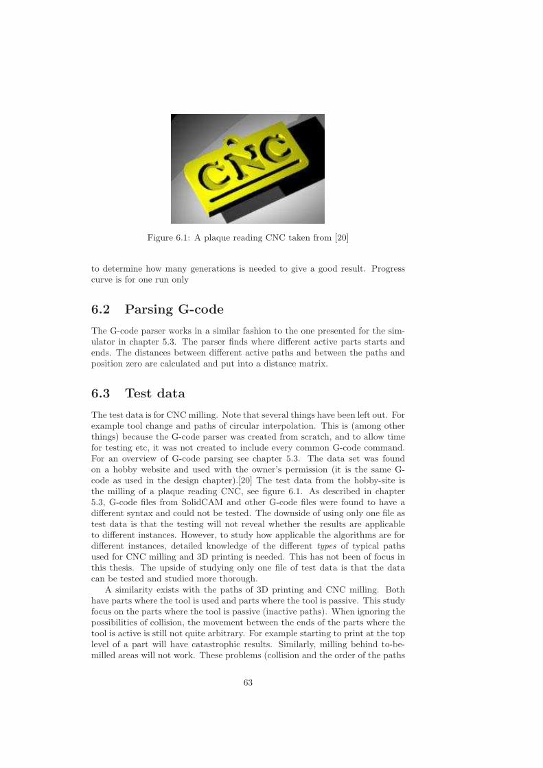
Figure 6.1: A plaque reading CNC taken from [20]

to determine how many generations is needed to give a good result. Progresscurve is for one run only

6.2 Parsing G-code

The G-code parser works in a similar fashion to the one presented for the sim-ulator in chapter 5.3. The parser finds where different active parts starts andends. The distances between different active paths and between the paths andposition zero are calculated and put into a distance matrix.

6.3 Test data

The test data is for CNCmilling. Note that several things have been left out. Forexample tool change and paths of circular interpolation. This is (among otherthings) because the G-code parser was created from scratch, and to allow timefor testing etc, it was not created to include every common G-code command.For an overview of G-code parsing see chapter 5.3. The data set was foundon a hobby website and used with the owner’s permission (it is the same G-code as used in the design chapter).[20] The test data from the hobby-site isthe milling of a plaque reading CNC, see figure 6.1. As described in chapter5.3, G-code files from SolidCAM and other G-code files were found to have adifferent syntax and could not be tested. The downside of using only one file astest data is that the testing will not reveal whether the results are applicableto different instances. However, to study how applicable the algorithms are fordifferent instances, detailed knowledge of the different types of typical pathsused for CNC milling and 3D printing is needed. This has not been of focus inthis thesis. The upside of studying only one file of test data is that the datacan be tested and studied more thorough.

A similarity exists with the paths of 3D printing and CNC milling. Bothhave parts where the tool is used and parts where the tool is passive. This studyfocus on the parts where the tool is passive (inactive paths). When ignoring thepossibilities of collision, the movement between the ends of the parts where thetool is active is still not quite arbitrary. For example starting to print at the toplevel of a part will have catastrophic results. Similarly, milling behind to-be-milled areas will not work. These problems (collision and the order of the paths

63

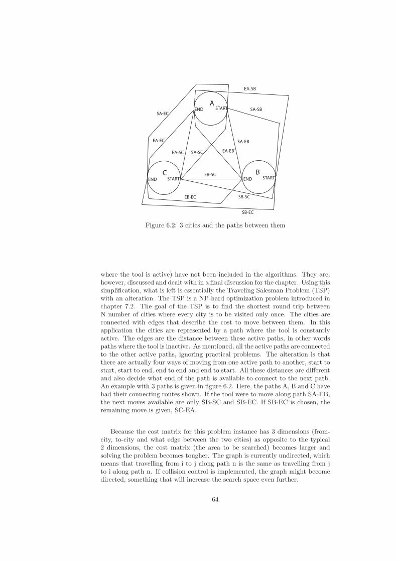
B

A

CSTART START

START

END END

END

EA-SB

SA-SB

SA-EB

EA-EBSA-SCEA-SC

SB-EC

SB-SCEB-EC

EB-SC

SA-EC

EA-EC

Figure 6.2: 3 cities and the paths between them

where the tool is active) have not been included in the algorithms. They are,however, discussed and dealt with in a final discussion for the chapter. Using thissimplification, what is left is essentially the Traveling Salesman Problem (TSP)with an alteration. The TSP is a NP-hard optimization problem introduced inchapter 7.2. The goal of the TSP is to find the shortest round trip betweenN number of cities where every city is to be visited only once. The cities areconnected with edges that describe the cost to move between them. In thisapplication the cities are represented by a path where the tool is constantlyactive. The edges are the distance between these active paths, in other wordspaths where the tool is inactive. As mentioned, all the active paths are connectedto the other active paths, ignoring practical problems. The alteration is thatthere are actually four ways of moving from one active path to another, start tostart, start to end, end to end and end to start. All these distances are differentand also decide what end of the path is available to connect to the next path.An example with 3 paths is given in figure 6.2. Here, the paths A, B and C havehad their connecting routes shown. If the tool were to move along path SA-EB,the next moves available are only SB-SC and SB-EC. If SB-EC is chosen, theremaining move is given, SC-EA.

Because the cost matrix for this problem instance has 3 dimensions (from-city, to-city and what edge between the two cities) as opposite to the typical2 dimensions, the cost matrix (the area to be searched) becomes larger andsolving the problem becomes tougher. The graph is currently undirected, whichmeans that travelling from i to j along path n is the same as travelling from jto i along path n. If collision control is implemented, the graph might becomedirected, something that will increase the search space even further.

64

6.4 Genetic Algorithm

For a general description of the genetic algorithm, see chapter 2.11. Whatfollows is a mapping from some of the standard operators used in the geneticalgorithm to this problem instance. The operators have been found in the book[19].

6.4.1 How it works - specific

Here, the details for the genetic algorithm used in this thesis are presented.Genetic algorithms are the most commonly known and most researched evolu-tionary algorithm.[19, p 37] The algorithm is created for each application withdifferent operators. The operators to define are:

• Representation of individuals

• Initialization operator

• Parent selection operator

• Crossover (recombination) operator

• Mutation operator

• Survivor selection mechanism

• Termination operator

Representation

The representation defines much of how the other operators are going to look likeand is therefore chosen first. For the travelling salesman problem, permutationrepresentation is the most common choice. The permutation can for example bea number where each digit represents a city or a list where each item representsa city. For the path-optimization problem presented here, the parsing of G-codeaffect what kind of representation can be used. As described in chapter 5.3, theparsing creates a list of paths, describing the start position, end position andthe type of movement. Each active path is given a number and the distancebetween them is stored in a cost matrix. Notice that between each path thereare 4 possible distances, so the cost matrix will have 3 dimensions. Since thereare four possible ways to move between two active paths and the selected optionaffect which way to move from the next active path, the path chosen between twocities have to be included in the representation. Therefore the representation ofan individual consists of a list of lists with two elements. Each list inside the listis made up of a number representing an active path/city and a second numberrepresenting the edge used between the current and the next path/city. For theedges, 0 represents a move from start of current to start of next, 1 represents amove from start to end, 2 represents from end to start and 3 represents from endof the current path to the end of the next path. An example of an individualwith the genes 1, 2 and 3: [[2, 1], [3, 0], [1, 3]]. Here the edge is from the startof path two to the end of path 3, from the start of path 3 to the start of path1 and from the end of path 1 to the end of path 2.

65

Initalisation

The initialization creates a number of random permutations that is equal to thepopulation size. Each individual is then given random edges between the activepaths (or genes or cities).

Parent selection

pi = q(1− q)i (6.1)

ai =i

∑

1

Psel(i) (6.2)

The population is first ranked according to their fitness and the equation(6.1).[17] A larger value for the parameter q, equals larger selection pressure.The equation gives each individual a probability of being chosen as a parent. Inthis algorithm the number of individuals (µ) is equal to the number of parents(λ). The number of offspring is equal to the number of parents. After eachindividual has had their probability calculated they are ranked from one (leastfit) to µ and given a value [a1, a2, ..., aµ] according to equation (6.2).[19, p 62]

Algorithm 1 beginset current member=i=1Pick a random value r uniformly from [0, 1/µ]while ( current member ≤ µ ) do

while ( r≤a[i ] ) do

set mating pool[current member ] = parents[i ]set r = r + 1/µset current member = current member+1

end while

set i = i+1end while

endPsueudocode fot the stochastic universal sampling (SUS) algorithm. Taken

from [19, p 60-63]

Parents are then selected according to the stochastic universal sampling(SUS) method.[19, p 60-63] This is similar to spinning a roulette wheel one timewith a number of equally spaced arms that is equal to the number of parentsthat are to be chosen. The pseudocode for SUS is presented in algorithm 1.

Crossover

There are mainly four crossover methods that are suitable for permutations,Partially Mapped Crossover (PMX), Edge Crossover, Order Crossover and CycleCrossover.[19, p 52-56] Of these, Eiben and Smith reports that PMX is the mostwidely used for adjacency-type problems such as the TSP. A slightly modifiedPMX has therefore been chosen as crossover operator. The modification hasbeen done because there are four possible edges between two genes and theedge used by the current gene is dependent on the edges used by the gene

66

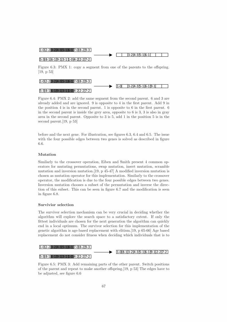
1-0 2-2 3-2 4-3 5-1 6-1 7-0 8-2 9-3

5-3 8-1 6-1 9-1 3-1 1-0 4-2 2-2 7-2

3-2 4-3 5-1 6-1

Figure 6.3: PMX 1: copy a segment from one of the parents to the offspring.[19, p 53]

1-0 2-2 3-2 4-3 5-1 6-1 7-0 8-2 9-3

5-3 8-1 6-1 9-1 3-1 1-0 4-2 2-2 7-2

3-2 4-3 5-1 6-1 9-11-0

Figure 6.4: PMX 2: add the same segment from the second parent. 6 and 3 arealready added and are ignored. 9 is opposite to 4 in the first parent. Add 9 inthe position 4 is in the second parent. 1 is opposite to 6 in the first parent. 6in the second parent is inside the grey area, opposite to 6 is 3, 3 is also in grayarea in the second parent. Opposite to 3 is 5, add 1 in the position 5 is in thesecond parent.[19, p 53]

before and the next gene. For illustration, see figures 6.3, 6.4 and 6.5. The issuewith the four possible edges between two genes is solved as described in figure6.6.

Mutation

Similarly to the crossover operation, Eiben and Smith present 4 common op-erators for mutating permutations, swap mutation, insert mutation, scramblemutation and inversion mutation.[19, p 45-47] A modified inversion mutation ischosen as mutation operator for this implementation. Similarly to the crossoveroperator, the modification is due to the four possible edges between two genes.Inversion mutation chooses a subset of the permutation and inverse the direc-tion of this subset. This can be seen in figure 6.7 and the modification is seenin figure 6.8.

Survivior selection

The survivor selection mechanism can be very crucial in deciding whether thealgorithm will explore the search space to a satisfactory extent. If only thefittest individuals are chosen for the next generation the algorithm can quicklyend in a local optimum. The survivor selection for this implementation of thegenetic algorithm is age-based replacement with elitism.[19, p 65-66] Age basedreplacement do not consider fitness when deciding which individuals that is to

1-0 2-2 3-2 4-3 5-1 6-1 7-0 8-2 9-3

5-3 8-1 6-1 9-1 3-1 1-0 4-2 2-2 7-2

3-2 4-3 5-1 6-1 9-1 2-2 7-21-0 8-1

Figure 6.5: PMX 3: Add remaining parts of the other parent. Switch positionsof the parent and repeat to make another offspring.[19, p 53] The edges have tobe adjusted, see figure 6.6

67

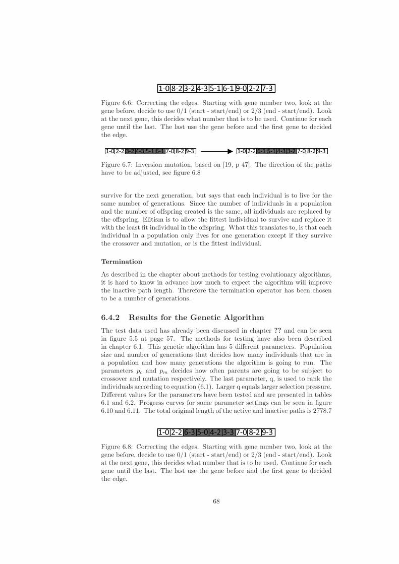
3-2 4-3 5-1 6-1 9-0 2-2 7-31-0 8-2

Figure 6.6: Correcting the edges. Starting with gene number two, look at thegene before, decide to use 0/1 (start - start/end) or 2/3 (end - start/end). Lookat the next gene, this decides what number that is to be used. Continue for eachgene until the last. The last use the gene before and the first gene to decidedthe edge.

1-0 2-2 6-1 5-1 4-3 3-2 7-0 8-2 9-31-0 2-2 3-2 4-3 5-1 6-1 7-0 8-2 9-3

Figure 6.7: Inversion mutation, based on [19, p 47]. The direction of the pathshave to be adjusted, see figure 6.8

survive for the next generation, but says that each individual is to live for thesame number of generations. Since the number of individuals in a populationand the number of offspring created is the same, all individuals are replaced bythe offspring. Elitism is to allow the fittest individual to survive and replace itwith the least fit individual in the offspring. What this translates to, is that eachindividual in a population only lives for one generation except if they survivethe crossover and mutation, or is the fittest individual.

Termination

As described in the chapter about methods for testing evolutionary algorithms,it is hard to know in advance how much to expect the algorithm will improvethe inactive path length. Therefore the termination operator has been chosento be a number of generations.

6.4.2 Results for the Genetic Algorithm

The test data used has already been discussed in chapter ?? and can be seenin figure 5.5 at page 57. The methods for testing have also been describedin chapter 6.1. This genetic algorithm has 5 different parameters. Populationsize and number of generations that decides how many individuals that are ina population and how many generations the algorithm is going to run. Theparameters pc and pm decides how often parents are going to be subject tocrossover and mutation respectively. The last parameter, q, is used to rank theindividuals according to equation (6.1). Larger q equals larger selection pressure.Different values for the parameters have been tested and are presented in tables6.1 and 6.2. Progress curves for some parameter settings can be seen in figure6.10 and 6.11. The total original length of the active and inactive paths is 2778.7

1-0 2-2 6-3 5-0 4-2 3-3 7-0 8-2 9-3

Figure 6.8: Correcting the edges. Starting with gene number two, look at thegene before, decide to use 0/1 (start - start/end) or 2/3 (end - start/end). Lookat the next gene, this decides what number that is to be used. Continue for eachgene until the last. The last use the gene before and the first gene to decidedthe edge.

68

mm. Of these is the tool active for 2508.9 mm and inactive for 269.8 mm. Ascan be seen, the inactive path is only 9-7% of the total lenght, something thatreally limits the path-length that can be saved.

Parameter setting 1 2 3 4 5 6 7 8 9 10 11Population size 100 100 100 100 100 100 25 25 500 60 60Generations 50 50 50 50 50 50 50 50 50 45 45pm 0.1 0.1 0.1 0.6 0.0 0.0 1.0 1.0 1.0 1.0 1.0pc 0.6 0.6 0.6 0.1 1.0 1.0 0.2 0.2 0.2 0.3 0.3q 0.5 0.5 0.5 0.5 0.5 0.5 0.5 0.5 0.5 0.5 0.5Runs 10 100 200 10 10 50 10 100 10 10 100

Table 6.1: Parameter settings for the different tests. Test results can be seen intable 6.2.

69

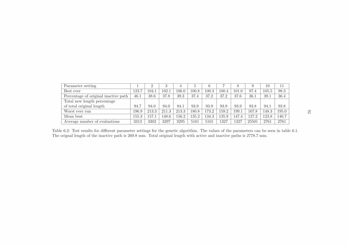
Parameter setting 1 2 3 4 5 6 7 8 9 10 11Best ever 123.7 104.1 102.1 106.0 100.8 100.3 100.4 101.0 97.4 105.5 98.3Percentage of original inactive path 46.1 38.6 37.8 39.3 37.4 37.2 37.2 37.6 36.1 39.1 36.4Total new length percentageof total original length 94.7 94.0 94.0 94.1 93.9 93.9 93.9 93.9 93.8 94.1 93.8Worst ever run 196.9 213.3 211.3 213.3 180.8 173.2 159.2 199.1 167.8 148.3 195.0Mean best 155.3 157.1 148.6 156.2 135.2 134.3 135.9 147.4 127.2 123.8 140.7Average number of evaluations 3313 3302 3297 3295 5101 5101 1327 1327 25501 2761 2761

Table 6.2: Test results for different parameter settings for the genetic algorithm. The values of the parameters can be seen in table 6.1.The orignal length of the inactive path is 269.8 mm. Total original length with active and inactive paths is 2778.7 mm.

70

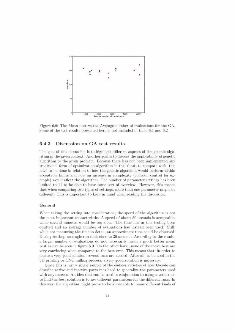
0 1000 2000 3000 4000 5000Average number of evaluations

0

50

100

150

200

Mean best

Figure 6.9: The Mean best vs the Average number of evaluations for the GA.Some of the test results presented here is not included in table 6.1 and 6.2

6.4.3 Discussion on GA test results

The goal of this discussion is to highlight different aspects of the genetic algo-rithm in the given context. Another goal is to discuss the applicability of geneticalgorithm to the given problem. Because there has not been implemented anytraditional form of optimization algorithm in this thesis to compare with, thishave to be done in relation to how the genetic algorithm would perform withinacceptable limits and how an increase in complexity (collision control for ex-ample) would affect the algorithm. The number of parameter settings has beenlimited to 11 to be able to have some sort of overview. However, this meansthat when comparing two types of settings, more than one parameter might bedifferent. This is important to keep in mind when reading the discussion.

General

When taking the setting into consideration, the speed of the algorithm is notthe most important characteristic. A speed of about 30 seconds is acceptable,while several minutes would be too slow. The time has in this testing beenomitted and an average number of evaluations has instead been used. Still,while not measuring the time in detail, an approximate time could be observed.During testing, no single run took close to 30 seconds. According to the resultsa larger number of evaluations do not necessarily mean a much better meanbest as can be seen in figure 6.9. On the other hand, none of the mean best arevery convincing when compared to the best ever. This means that, in order tolocate a very good solution, several runs are needed. After all, to be used in the3D printing or CNC milling process, a very good solution is necessary.

Since this is just a single sample of the endless varieties of how G-code candescribe active and inactive parts it is hard to generalize the parameters usedwith any success. An idea that can be used in conjunction to using several runsto find the best solution is to use different parameters for the different runs. Inthis way, the algorithm might prove to be applicable to many different kinds of

71

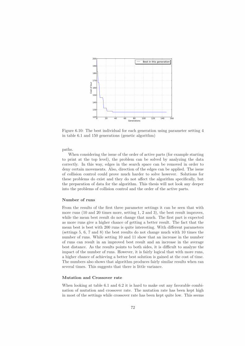
0 20 40 60 80 100 120 140 160Generations

120

130

140

150

160

170

180

190

200

Cost of tour

Best in this generation

Figure 6.10: The best individual for each generation using parameter setting 4in table 6.1 and 150 generations (genetic algorithm)

paths.When considering the issue of the order of active parts (for example starting

to print at the top level), the problem can be solved by analyzing the datacorrectly. In this way, edges in the search space can be removed in order todeny certain movements. Also, direction of the edges can be applied. The issueof collision control could prove much harder to solve however. Solutions forthese problems do exist and they do not affect the algorithm specifically, butthe preparation of data for the algorithm. This thesis will not look any deeperinto the problems of collision control and the order of the active parts.

Number of runs

From the results of the first three parameter settings it can be seen that withmore runs (10 and 20 times more, setting 1, 2 and 3), the best result improves,while the mean best result do not change that much. The first part is expectedas more runs give a higher chance of getting a better result. The fact that themean best is best with 200 runs is quite interesting. With different parameters(settings 5, 6, 7 and 8) the best results do not change much with 10 times thenumber of runs. While setting 10 and 11 show that an increase in the numberof runs can result in an improved best result and an increase in the averagebest distance. As the results points to both sides, it is difficult to analyze theimpact of the number of runs. However, it is fairly logical that with more runs,a higher chance of achieving a better best solution is gained at the cost of time.The numbers also shows that algorithm produces fairly similar results when ranseveral times. This suggests that there is little variance.

Mutation and Crossover rate

When looking at table 6.1 and 6.2 it is hard to make out any favorable combi-nation of mutation and crossover rate. The mutation rate has been kept highin most of the settings while crossover rate has been kept quite low. This seems

72

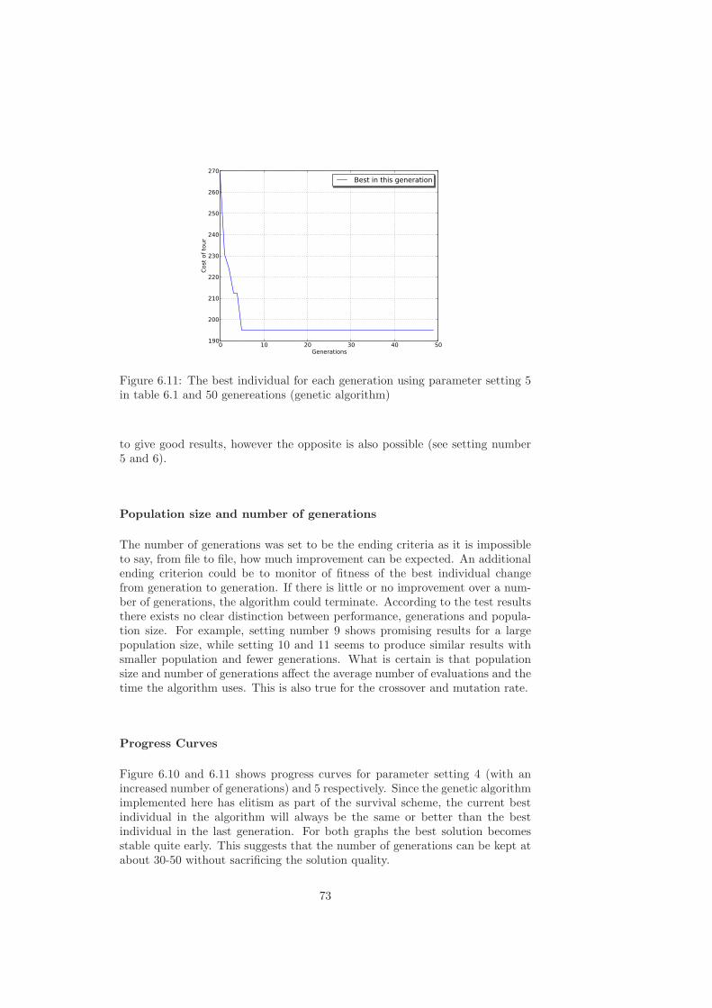
0 10 20 30 40 50Generations

190

200

210

220

230

240

250

260

270

Cost of tour

Best in this generation

Figure 6.11: The best individual for each generation using parameter setting 5in table 6.1 and 50 genereations (genetic algorithm)

to give good results, however the opposite is also possible (see setting number5 and 6).

Population size and number of generations

The number of generations was set to be the ending criteria as it is impossibleto say, from file to file, how much improvement can be expected. An additionalending criterion could be to monitor of fitness of the best individual changefrom generation to generation. If there is little or no improvement over a num-ber of generations, the algorithm could terminate. According to the test resultsthere exists no clear distinction between performance, generations and popula-tion size. For example, setting number 9 shows promising results for a largepopulation size, while setting 10 and 11 seems to produce similar results withsmaller population and fewer generations. What is certain is that populationsize and number of generations affect the average number of evaluations and thetime the algorithm uses. This is also true for the crossover and mutation rate.

Progress Curves

Figure 6.10 and 6.11 shows progress curves for parameter setting 4 (with anincreased number of generations) and 5 respectively. Since the genetic algorithmimplemented here has elitism as part of the survival scheme, the current bestindividual in the algorithm will always be the same or better than the bestindividual in the last generation. For both graphs the best solution becomesstable quite early. This suggests that the number of generations can be kept atabout 30-50 without sacrificing the solution quality.

73

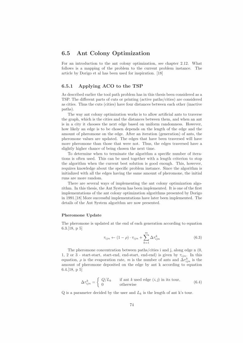
6.5 Ant Colony Optimization

For an introduction to the ant colony optimization, see chapter 2.12. Whatfollows is a mapping of the problem to the current problem instance. Thearticle by Dorigo et al has been used for inspiration. [18]

6.5.1 Applying ACO to the TSP

As described earlier the tool path problem has in this thesis been considered as aTSP. The different parts of cuts or printing (active paths/cities) are consideredas cities. Thus the cuts (cities) have four distances between each other (inactivepaths).

The way ant colony optimization works is to allow artificial ants to traversethe graph, which is the cities and the distances between them, and when an antis in a city it chooses the next edge based on uniform randomness. However,how likely an edge is to be chosen depends on the length of the edge and theamount of pheromone on the edge. After an iteration (generation) of ants, thepheromone values are updated. The edges that have been traversed will havemore pheromone than those that were not. Thus, the edges traversed have aslightly higher chance of being chosen the next time.

To determine when to terminate the algorithm a specific number of itera-tions is often used. This can be used together with a length criterion to stopthe algorithm when the current best solution is good enough. This, however,requires knowledge about the specific problem instance. Since the algorithm isinitialized with all the edges having the same amount of pheromone, the initialruns are more random.

There are several ways of implementing the ant colony optimization algo-rithm. In this thesis, the Ant System has been implemented. It is one of the firstimplementations of the ant colony optimization algorithms presented by Dorigoin 1991.[18] More successful implementations have later been implemented. Thedetails of the Ant System algorithm are now presented.

Pheromone Update

The pheromone is updated at the end of each generation according to equation6.3.[18, p 5]

τijn ← (1− ρ) · τijn +

m∑

k=1

∆τkijn (6.3)

The pheromone concentration between paths/cities i and j, along edge n (0,1, 2 or 3 - start-start, start-end, end-start, end-end) is given by τijn. In thisequation, ρ is the evaporation rate, m is the number of ants and ∆τkijn is theamount of pheromone deposited on the edge by ant k according to equation6.4.[18, p 5]

∆τkijn =

{

Q/Lk if ant k used edge (i, j) in its tour,0 otherwise

(6.4)

Q is a parameter decided by the user and Lk is the length of ant k’s tour.

74

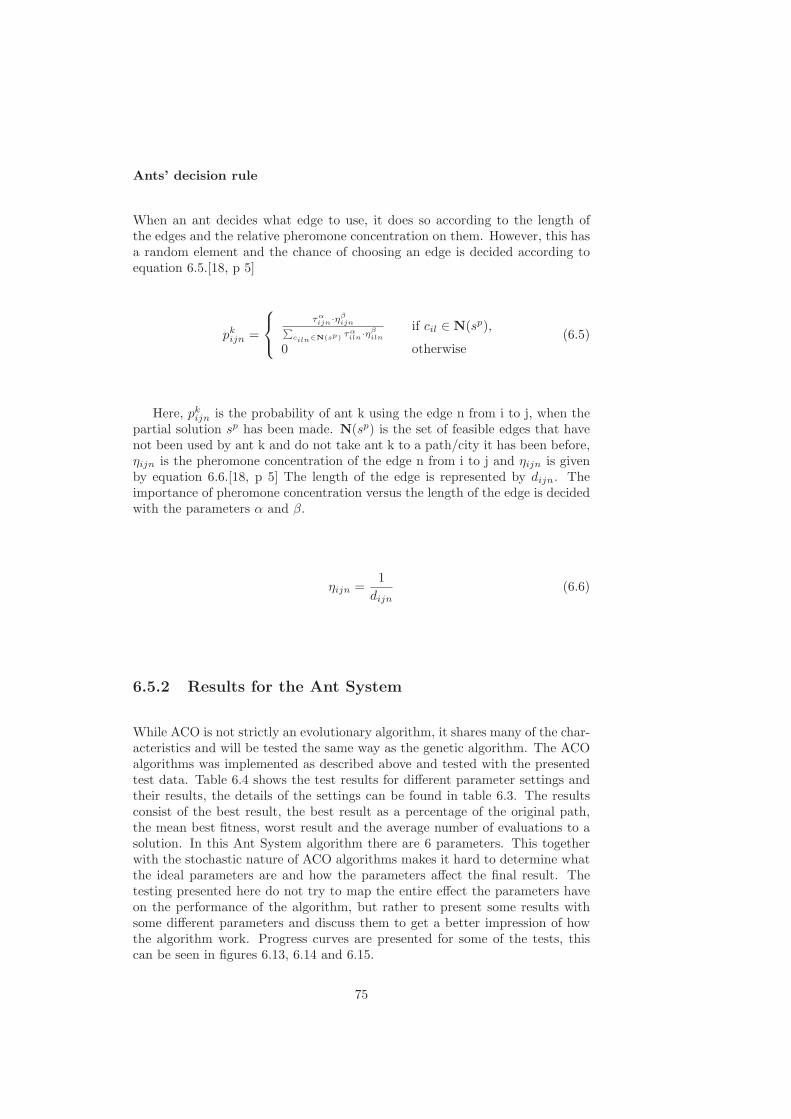
Ants’ decision rule

When an ant decides what edge to use, it does so according to the length ofthe edges and the relative pheromone concentration on them. However, this hasa random element and the chance of choosing an edge is decided according toequation 6.5.[18, p 5]

pkijn =

ταijn·η

βijn

∑

ciln∈N(sp) ταiln·η

βiln

if cil ∈ N(sp),

0 otherwise(6.5)

Here, pkijn is the probability of ant k using the edge n from i to j, when thepartial solution sp has been made. N(sp) is the set of feasible edges that havenot been used by ant k and do not take ant k to a path/city it has been before,ηijn is the pheromone concentration of the edge n from i to j and ηijn is givenby equation 6.6.[18, p 5] The length of the edge is represented by dijn. Theimportance of pheromone concentration versus the length of the edge is decidedwith the parameters α and β.

ηijn =1

dijn(6.6)

6.5.2 Results for the Ant System

While ACO is not strictly an evolutionary algorithm, it shares many of the char-acteristics and will be tested the same way as the genetic algorithm. The ACOalgorithms was implemented as described above and tested with the presentedtest data. Table 6.4 shows the test results for different parameter settings andtheir results, the details of the settings can be found in table 6.3. The resultsconsist of the best result, the best result as a percentage of the original path,the mean best fitness, worst result and the average number of evaluations to asolution. In this Ant System algorithm there are 6 parameters. This togetherwith the stochastic nature of ACO algorithms makes it hard to determine whatthe ideal parameters are and how the parameters affect the final result. Thetesting presented here do not try to map the entire effect the parameters haveon the performance of the algorithm, but rather to present some results withsome different parameters and discuss them to get a better impression of howthe algorithm work. Progress curves are presented for some of the tests, thiscan be seen in figures 6.13, 6.14 and 6.15.

75

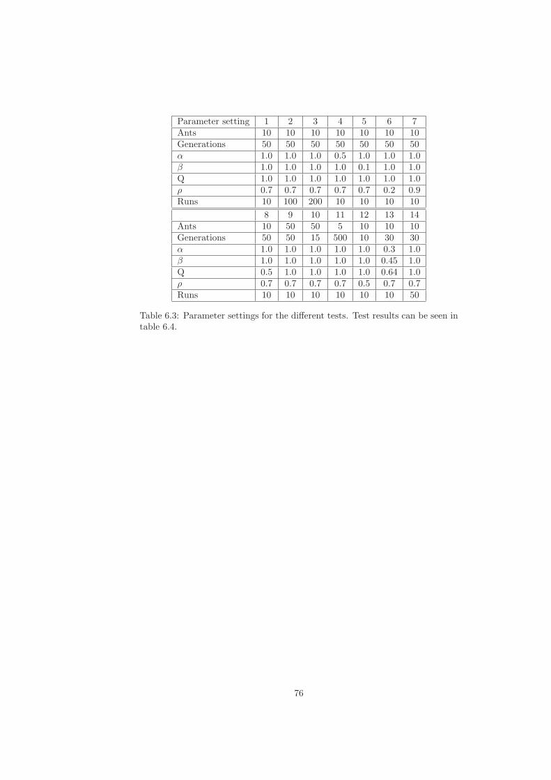
Parameter setting 1 2 3 4 5 6 7Ants 10 10 10 10 10 10 10Generations 50 50 50 50 50 50 50α 1.0 1.0 1.0 0.5 1.0 1.0 1.0β 1.0 1.0 1.0 1.0 0.1 1.0 1.0Q 1.0 1.0 1.0 1.0 1.0 1.0 1.0ρ 0.7 0.7 0.7 0.7 0.7 0.2 0.9Runs 10 100 200 10 10 10 10

8 9 10 11 12 13 14Ants 10 50 50 5 10 10 10Generations 50 50 15 500 10 30 30α 1.0 1.0 1.0 1.0 1.0 0.3 1.0β 1.0 1.0 1.0 1.0 1.0 0.45 1.0Q 0.5 1.0 1.0 1.0 1.0 0.64 1.0ρ 0.7 0.7 0.7 0.7 0.5 0.7 0.7Runs 10 10 10 10 10 10 50

Table 6.3: Parameter settings for the different tests. Test results can be seen intable 6.4.

76

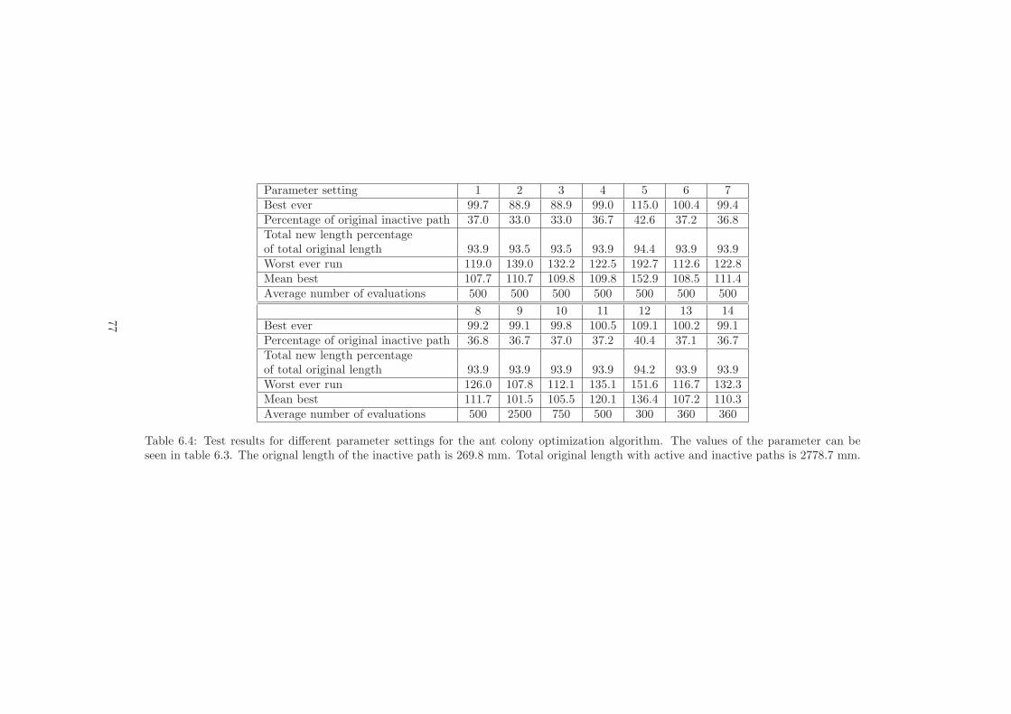
Parameter setting 1 2 3 4 5 6 7Best ever 99.7 88.9 88.9 99.0 115.0 100.4 99.4Percentage of original inactive path 37.0 33.0 33.0 36.7 42.6 37.2 36.8Total new length percentageof total original length 93.9 93.5 93.5 93.9 94.4 93.9 93.9Worst ever run 119.0 139.0 132.2 122.5 192.7 112.6 122.8Mean best 107.7 110.7 109.8 109.8 152.9 108.5 111.4Average number of evaluations 500 500 500 500 500 500 500

8 9 10 11 12 13 14Best ever 99.2 99.1 99.8 100.5 109.1 100.2 99.1Percentage of original inactive path 36.8 36.7 37.0 37.2 40.4 37.1 36.7Total new length percentageof total original length 93.9 93.9 93.9 93.9 94.2 93.9 93.9Worst ever run 126.0 107.8 112.1 135.1 151.6 116.7 132.3Mean best 111.7 101.5 105.5 120.1 136.4 107.2 110.3Average number of evaluations 500 2500 750 500 300 360 360

Table 6.4: Test results for different parameter settings for the ant colony optimization algorithm. The values of the parameter can beseen in table 6.3. The orignal length of the inactive path is 269.8 mm. Total original length with active and inactive paths is 2778.7 mm.

77

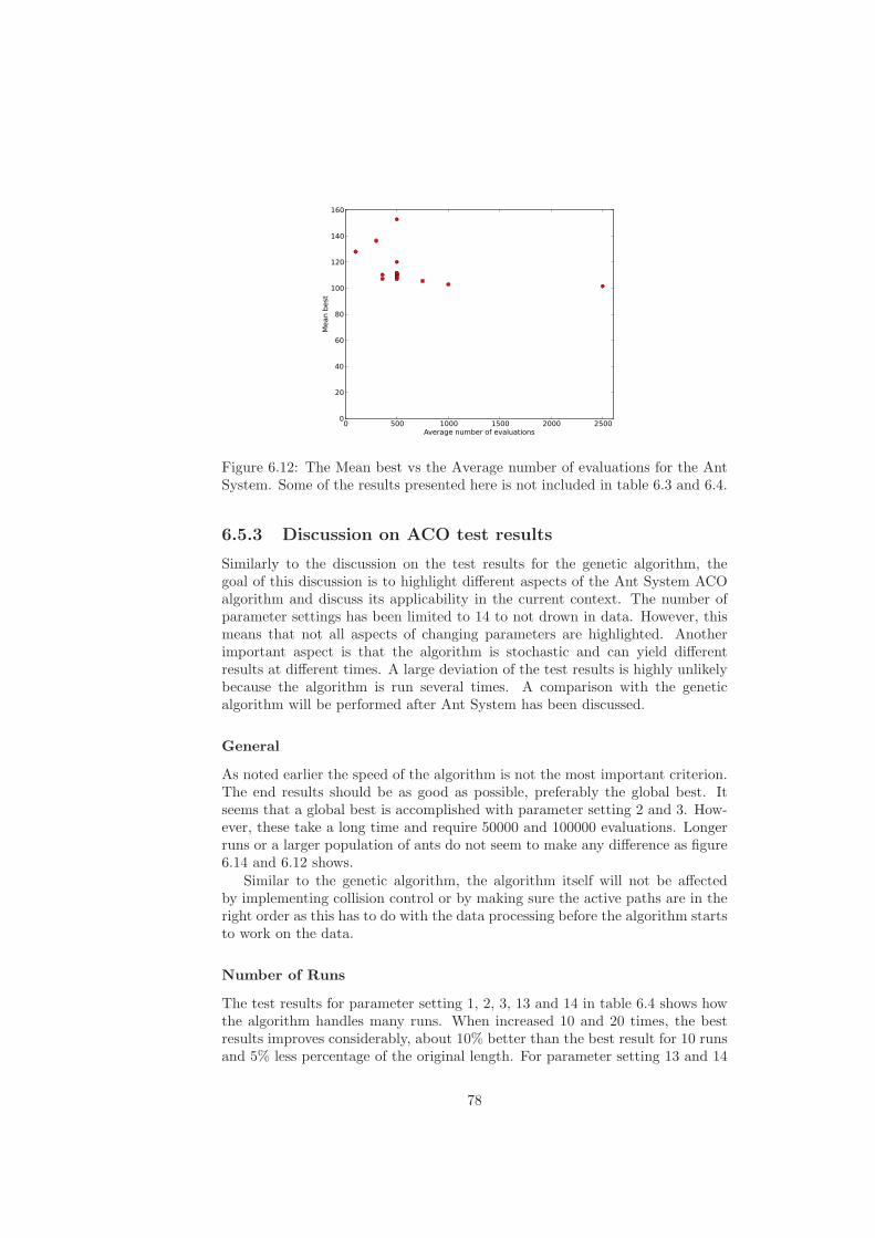
0 500 1000 1500 2000 2500Average number of evaluations

0

20

40

60

80

100

120

140

160

Mean best

Figure 6.12: The Mean best vs the Average number of evaluations for the AntSystem. Some of the results presented here is not included in table 6.3 and 6.4.

6.5.3 Discussion on ACO test results

Similarly to the discussion on the test results for the genetic algorithm, thegoal of this discussion is to highlight different aspects of the Ant System ACOalgorithm and discuss its applicability in the current context. The number ofparameter settings has been limited to 14 to not drown in data. However, thismeans that not all aspects of changing parameters are highlighted. Anotherimportant aspect is that the algorithm is stochastic and can yield differentresults at different times. A large deviation of the test results is highly unlikelybecause the algorithm is run several times. A comparison with the geneticalgorithm will be performed after Ant System has been discussed.

General

As noted earlier the speed of the algorithm is not the most important criterion.The end results should be as good as possible, preferably the global best. Itseems that a global best is accomplished with parameter setting 2 and 3. How-ever, these take a long time and require 50000 and 100000 evaluations. Longerruns or a larger population of ants do not seem to make any difference as figure6.14 and 6.12 shows.

Similar to the genetic algorithm, the algorithm itself will not be affectedby implementing collision control or by making sure the active paths are in theright order as this has to do with the data processing before the algorithm startsto work on the data.

Number of Runs

The test results for parameter setting 1, 2, 3, 13 and 14 in table 6.4 shows howthe algorithm handles many runs. When increased 10 and 20 times, the bestresults improves considerably, about 10% better than the best result for 10 runsand 5% less percentage of the original length. For parameter setting 13 and 14

78

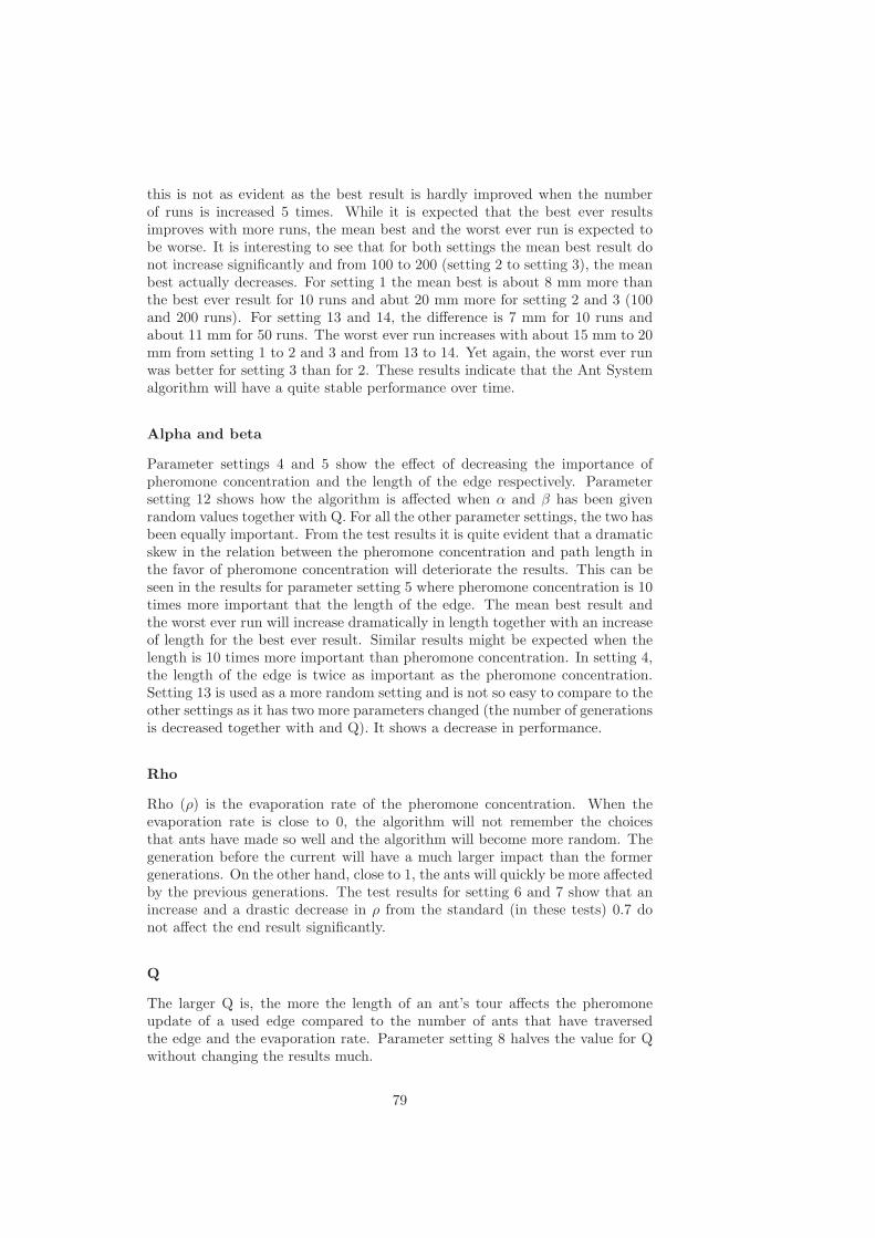
this is not as evident as the best result is hardly improved when the numberof runs is increased 5 times. While it is expected that the best ever resultsimproves with more runs, the mean best and the worst ever run is expected tobe worse. It is interesting to see that for both settings the mean best result donot increase significantly and from 100 to 200 (setting 2 to setting 3), the meanbest actually decreases. For setting 1 the mean best is about 8 mm more thanthe best ever result for 10 runs and abut 20 mm more for setting 2 and 3 (100and 200 runs). For setting 13 and 14, the difference is 7 mm for 10 runs andabout 11 mm for 50 runs. The worst ever run increases with about 15 mm to 20mm from setting 1 to 2 and 3 and from 13 to 14. Yet again, the worst ever runwas better for setting 3 than for 2. These results indicate that the Ant Systemalgorithm will have a quite stable performance over time.

Alpha and beta

Parameter settings 4 and 5 show the effect of decreasing the importance ofpheromone concentration and the length of the edge respectively. Parametersetting 12 shows how the algorithm is affected when α and β has been givenrandom values together with Q. For all the other parameter settings, the two hasbeen equally important. From the test results it is quite evident that a dramaticskew in the relation between the pheromone concentration and path length inthe favor of pheromone concentration will deteriorate the results. This can beseen in the results for parameter setting 5 where pheromone concentration is 10times more important that the length of the edge. The mean best result andthe worst ever run will increase dramatically in length together with an increaseof length for the best ever result. Similar results might be expected when thelength is 10 times more important than pheromone concentration. In setting 4,the length of the edge is twice as important as the pheromone concentration.Setting 13 is used as a more random setting and is not so easy to compare to theother settings as it has two more parameters changed (the number of generationsis decreased together with and Q). It shows a decrease in performance.

Rho

Rho (ρ) is the evaporation rate of the pheromone concentration. When theevaporation rate is close to 0, the algorithm will not remember the choicesthat ants have made so well and the algorithm will become more random. Thegeneration before the current will have a much larger impact than the formergenerations. On the other hand, close to 1, the ants will quickly be more affectedby the previous generations. The test results for setting 6 and 7 show that anincrease and a drastic decrease in ρ from the standard (in these tests) 0.7 donot affect the end result significantly.

Q

The larger Q is, the more the length of an ant’s tour affects the pheromoneupdate of a used edge compared to the number of ants that have traversedthe edge and the evaporation rate. Parameter setting 8 halves the value for Qwithout changing the results much.

79

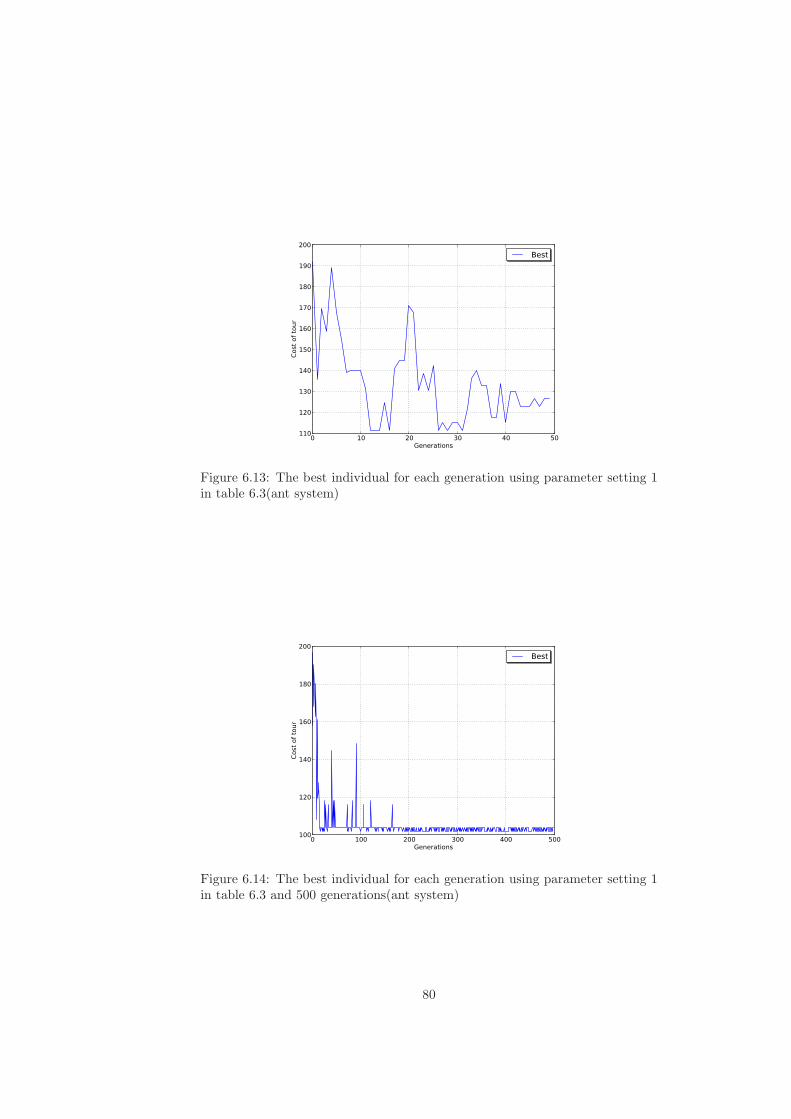
0 10 20 30 40 50Generations

110

120

130

140

150

160

170

180

190

200

Cost of tour

Best

Figure 6.13: The best individual for each generation using parameter setting 1in table 6.3(ant system)

0 100 200 300 400 500Generations

100

120

140

160

180

200

Cost of tour

Best

Figure 6.14: The best individual for each generation using parameter setting 1in table 6.3 and 500 generations(ant system)

80

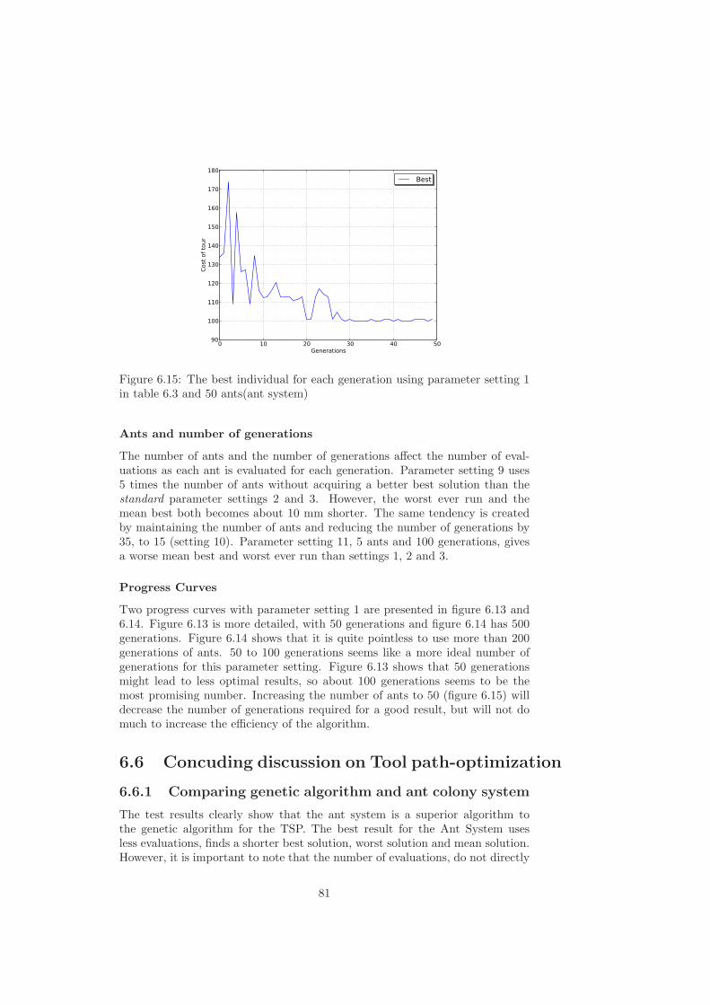
0 10 20 30 40 50Generations

90

100

110

120

130

140

150

160

170

180

Cost of tour

Best

Figure 6.15: The best individual for each generation using parameter setting 1in table 6.3 and 50 ants(ant system)

Ants and number of generations

The number of ants and the number of generations affect the number of eval-uations as each ant is evaluated for each generation. Parameter setting 9 uses5 times the number of ants without acquiring a better best solution than thestandard parameter settings 2 and 3. However, the worst ever run and themean best both becomes about 10 mm shorter. The same tendency is createdby maintaining the number of ants and reducing the number of generations by35, to 15 (setting 10). Parameter setting 11, 5 ants and 100 generations, givesa worse mean best and worst ever run than settings 1, 2 and 3.

Progress Curves

Two progress curves with parameter setting 1 are presented in figure 6.13 and6.14. Figure 6.13 is more detailed, with 50 generations and figure 6.14 has 500generations. Figure 6.14 shows that it is quite pointless to use more than 200generations of ants. 50 to 100 generations seems like a more ideal number ofgenerations for this parameter setting. Figure 6.13 shows that 50 generationsmight lead to less optimal results, so about 100 generations seems to be themost promising number. Increasing the number of ants to 50 (figure 6.15) willdecrease the number of generations required for a good result, but will not domuch to increase the efficiency of the algorithm.

6.6 Concuding discussion on Tool path-optimization

6.6.1 Comparing genetic algorithm and ant colony system

The test results clearly show that the ant system is a superior algorithm tothe genetic algorithm for the TSP. The best result for the Ant System usesless evaluations, finds a shorter best solution, worst solution and mean solution.However, it is important to note that the number of evaluations, do not directly

81

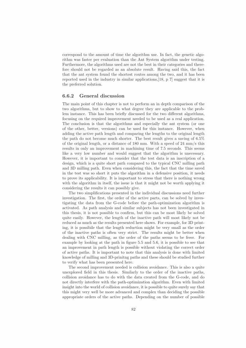
correspond to the amount of time the algorithm use. In fact, the genetic algo-rithm was faster per evaluation than the Ant System algorithm under testing.Furthermore, the algorithms used are not the best in their categories and there-fore should not be regarded as an absolute result. Having said this, the factthat the ant system found the shortest routes among the two, and it has beenreported used in the industry in similar applications,[18, p 7] suggest that it isthe preferred solution.

6.6.2 General discussion

The main point of this chapter is not to perform an in depth comparison of thetwo algorithms, but to show to what degree they are applicable to the prob-lem instance. This has been briefly discussed for the two different algorithms,focusing on the required improvement needed to be used as a real application.The conclusion is that the algorithms and especially the ant system (or oneof the other, better, versions) can be used for this instance. However, whenadding the active path length and comparing the lengths to the original lengththe path do not become much shorter. The best result gives a saving of 6.5%of the original length, or a distance of 180 mm. With a speed of 24 mm/s thisresults in only an improvement in machining time of 7.5 seconds. This seemslike a very low number and would suggest that the algorithm is unecessary.However, it is important to consider that the test data is an inscription of adesign, which is a quite short path compared to the typical CNC milling pathand 3D milling path. Even when considering this, the fact that the time savedin the test was so short it puts the algorithm in a defensive position, it needsto prove its applicability. It is important to stress that there is nothing wrongwith the algorithm in itself, the issue is that it might not be worth applying itconsidering the results it can possibly give.

The two simplifications presented in the individual discussions need furtherinvestigation. The first, the order of the active parts, can be solved by inves-tigating the data from the G-code before the path-optimization algorithm isactivated. As path analysis and similar subjects has not been investigated inthis thesis, it is not possible to confirm, but this can be most likely be solvedquite easily. However, the length of the inactive path will most likely not bereduced as much as the results presented here shows. For example, for 3D print-ing, it is possibile that the length reduction might be very small as the orderof the inactive paths is often very strict. The results might be better whendealing with CNC milling, as the order of the paths seems to be freer. Forexample by looking at the path in figure 5.5 and 5.6, it is possible to see thatan improvement in path length is possible without violating the correct orderof active paths. It is important to note that this analysis is done with limitedknowledge of milling and 3D-prinitng paths and these should be studied furtherto verify what has been presented here.

The second improvement needed is collision avoidance. This is also a quiteunexplored field in this thesis. Similarly to the order of the inactive paths,collision avoidance has to do with the data created from the G-code, and donot directly interfere with the path-optimization algorithm. Even with limitedinsight into the world of collision avoidance, it is possible to quite surely say thatthis might very well be more advanced and complex than deciding the possibleappropriate orders of the active paths. Depending on the number of possible

82

inactive paths, it might prove too time consuming to analyze all the paths inorder to deny collisions and calculate the lengths. However, it might be so thatnot all the possible inactive paths will be explored in the path-optimizationalgorithm. To exploit this, the length of collision free inactive paths might becalculated while running the path-optimization algorithm. A study of how manyof the possible inactive paths explored by the algorithms can show whether thisexploitation is possible. It seems that the inclusion of collision avoidance canbe one of the central problems of further development.

An issue, which has been mentioned, is that when these simplifications areimproved, the path found by the algorithm might very well not be shortened asmuch as the current test results suggests. This is also affected by the type ofpath to be improved (different G-code files, different types of tool path) and itis very hard to determine the total effect the algorithms has before testing onmany different paths.

To conclude, the current problem do not so much lie with the algorithmsas the preparation of data for the algorithm and the possible length that canbe saved by analyzing the inactive paths. In this way, it is possible to saythat the ant system algorithm and to some degree, the genetic algorithm, isapplicable to the problem instance. However, the issue of preparing the dataproperly might prove to be too time consuming, making the algorithms efficiencyfutile. Further investigation of data preparation can reveal this. Another aspectis that the improvements might render the algorithm less efficient by denyingmuch improvement in the inactive path length. There are still some hurdlesthat need to be jumped.

83

Chapter 7

Conclusion and proposals

for further work

7.1 Conclusion

Working with this thesis has been an immense learning experience. The areasto study that are related to robotic manipulators are many and varied. Thismeant that not all the areas could be explored as much as desired. I have gainedinsight into the design issues for a Stewart platform, studied G-code and themathematics behind the platform to create a simulator. These studies allowedme to analyze the properties of tool paths and discover how to improve thelength of them. Other topics have also been to some extent studied, such as thetravelling salesman problem and biologically inspired computing. The differentapproaches of design, simulation and path-optimization really allowed me tounderstand the problems and the Stewart platform better. The thesis allowedmore than anything to get to know the Stewart platform in detail.

What follows is a short conclusion of the three aspects of this thesis. Theseare the design, the simulation and the path-optimization using biologically in-spired computing. Then the experience from the three parts is put togetherto evaluate the possibility of using the Stewart platform as a rapid prototyperalternative to the current RepRap design (Mendel) that can both perform 3Dprinting and CNC milling. There are several aspects to this project, for examplethe issues regarding implementing the system to test it in a practical manner.Another aspect is studying areas of research that are related to the system, suchas workspace analysis.

Design The design chapter explored how a rapid prototyper with 3D print-ing and CNC milling capabilities could be physically implemented as a Stewartplatform, looked at issues such as workspace limitations and the design of anactuator and compared the design with the RepRap Mendel. Further studiesand practical testing is needed to verify whether the presented design will con-tain the presented characteristics. The design that shows the most interestingcapabilities is the third experimental design. A figure of this design can beseen at page 45 (figure 4.19). Goal number 1 as presented in chapter 1.2 hasthus been achieved. No future problems were found too large or complex to be

85

solved, and thus further study and testing of the design is encouraged.

Simulator The simulator has capabilities to perform simple analysis of howthe Stewart platform behaves according to a G-code file. The path can also bestudied to be verified. Due to the fact that there is no standard G-code syntaxand in order to make a working version of the manipulator, not all types ofG-code files and commands were implemented. Further development in thesefields, especially the amount of commands handled, is needed. To do this, thestyle of the G-code needs to be decided. The creation of the simulator enabledme to better understand the Stewart platform, CNC-milling and 3D printing.In this way, goal number 2 as presented in chapter 1.2 has been achieved.

Biologically inspired path-optimization Both the genetic algorithm andthe ACO algorithm managed to improve the inactive parts of the tool path to lessthan half the length of the original inactive path lengths. The ACO algorithmgave consistently better results. Since there were made two very importantsimplifications, these have to be studied before the algorithm actually can beapplied on the problem instance. The two simplifications lies in how the datais treated before entering the algorithm, therefore the current challenge is notin the algorithm, but in the preparation of data. Improving the simplificationscan also make the algorithms less efficient by denying shorter paths. Maybe themost important aspect of this study is that the best result only decreases themachining time with 7.5 seconds when the fast speed is set to 24 mm/s. Thetool path-optimization problem has thusly been investigated and algorithmshave been implemented to solve it as described as goal 3 in chapter 1.2.

The Stewart Platofrm as a Rapid Prototyper The overlying goal wasto investigate whether a robotic manipulator could be an alternative to theMendel RepRap with improved functionality. At the present stage, the study ofthe Stewart platform can not dismiss its use as a rapid prototyper and RepRapalternative. The final conclusion is that there are several positive indicationsthat the Stewart platform can be a very good alternative to the RepRap. Butthere are some problems (for example speed) that might deny such a possibility.The problems have to be solved and the positive indications tested further inorder to confirm the possibility to use the Stewart platform as a rapid proto-typer.

7.2 Further Work

Further work is suggestions for research topics that became evident during thework with this thesis. Since the area of study has been so wide, many differenttopics can be studied and therefore the number of topics presented here do notinclude everything that came up while working on this master thesis.

Avoid singularities and workspace Singularities for the Stewart platformare positions and orientations where the manipulator gains one degree of freedomand becomes uncontrollable. A complete description and characterization of thesingularities would be to parameterize the entire singularity hyper-surface(s)

86

in the task-space (6D in the case of the Stewart platform).[14] Then, all thesingularities can be analytically identified. This is however extremely difficultand Bhaskar Dasgupta and T.S. Mruthyunjaya had in 1998 not seen any workon work on this topic.

They had however found some practical work on the issue. Bhattacharyaet al. [14] have looked at paths in vicinity of a singularity and Dasgupta andMruthyunjaya themselves have studied singularity avoidance between two po-sitions. Later researches have also been performed, such as Qimi Jiang andClment M. Gosselin’s study from 2009.[26] Singularity avoidance is importantfor controlling the Stewart platform to avoid uncontrollable situations. Furtherstudy of the theoretical and analytical solutions is needed. Another issue is toimplement current solutions of singularity avoidance on the system presented inthis thesis. Singularities are tightly connected with the workspace as singularpositions are positions that limit the workspace. Studying the workspace of aStewart platform is also a possible research topic.

Controlling the Stewart Platform In addition to avoiding singularities,avoiding collisions is important. There are two aspects of collision avoidance.The typical one is to avoid colliding with objects in the vicinity of the manip-ulator (such as the part that the machine is milling on). And the second onis to avoid colliding with the manipulators own parts as discussed in chapter4.5.1. As collision avoidance is outside the scope of this thesis, it’s details hasnot been studied. Studies relating to collision control of the Stewart platforminclude [11], while for a study of a more general collision control of robotics, seefor example [28], [58, ch. 5] or [12, ch. 7]. Implementing this theory on the pre-sented Stewart platform can be interesting. Taking this a step further would beto study the extra complexity in avoiding collisions due to experimental designnumber 3. Also needed for controlling the manipulator is a G-code parser thatunderstand most of or all the G-code commands.

Path-optimization This has already been somewhat discussed in the finalconclusion. Collision avoidance, singularity avoidance and correct order of pathneed to be treated in order for the path-optimization algorithms to be applicable.Other aspects that can be studied are the possibility of dividing active paths inorder to shorten the total path length even further. Furthermore, testing the al-gorithms on more G-code files should be done to find out whether a considerableamount of time can be saved by using this type of path-optimization. In orderto do this conscientiously, a study and identification of different types of G-codepaths should be performed. Even more important is to study several G-codefiles to investigate the lengths of the inactive paths. This should be done to findout whether applicating path-optimization on the inactive paths would in anycase save a considerable amount of machining time. Another topic that was notfound in the literature is to compare the biologically inspired path-optimizationalgorithms with non-biological alternatives. Yet an even more interesting optioncould be to combine the studies done with traditional algorithms and biologi-cally inspired algorithms.

Building, testing and simulation One of the long term goals initiated bythis thesis is to create an alternative to the RepRap. In order to do this, the

87

Stewart platform needs to be built and tested. An interesting test would beto find out how many percentage of itself the manipulator can create. Anotheris to test the rigidity of the platform. Many of the issues that have been dis-cussed above have to be implemented before this can be done, such as avoidingcollisions and singularities and creating a control system that includes moreG-commands. As the control system is closely related to the simulator, thisalso gives a chance to improve the simulator. Furthermore, the simulator canbe improved in other ways, such as including the shape of the platform parts.Another two issues are testing the different parts for durability and finding outwhether the experimental design is realizable.

88

Bibliography

[1] Arduino homepage. http://www.arduino.cc/(2011-04-28).

[2] Charles Bates. Move over machine tools here come robots. http://www.

americanmachinist.com/304/Issue/Article/False/13386/(2010-03-26), 02 2006.

[3] K.A. Berman and J.L. Paul. Algorithms: sequential, parallel, and dis-tributed. Thomson/Course Technology, 2005.

[4] E. Bohez, S.S. Makhanov, and K. Sonthipermpoon. Adaptive nonlineartool path optimization for five-axis machining. International Journal ofProduction Research, 38(17):4329–4343, 2000.

[5] I.A. Bonev and J. Ryu. A new approach to orientation workspace analysis of6-DOF parallel manipulators. Mechanism and Machine Theory, 36(1):15–28, 2001.

[6] Adrian Bowyer. A self-copying manufacturing process. http://www.

reprap.org/pub/Main/WebHome/one-page.pdf(2010-03-24).

[7] A. W. (editor) Burks and John von Neumann. Theory of Self-ReproducingAutomata. University of Illinois Press, Urbana, Illinois, USA, 1966.Von Neumann’s work on self-reproducing automata, completed and editedafter his death by Arthur Burks. Also includes transcripts of von Nuemann’s1949 University of Illinois lectures on the “Theory and Organization ofComplicated Automata”.

[8] Z. Car, B. Barisic, and M. Ikonic. GA based CNC turning center exploita-tion process parameters optimization. Metalurgija, 48(1):47–50, 2009.

[9] J.N. Chiasson. Modeling and high performance control of electric machines.IEEE Press series on power engineering. John Wiley, 2005.

[10] Commercial 3d printer used: Dimension 768 se-ries. http://www.dimensionprinting.com/3d-printers/

printing-productspecs768series.aspx(2011-04-30).

[11] J. Cortes and T. Simeon. Probabilistic motion planning for parallel mech-anisms. In Robotics and Automation, 2003. Proceedings. ICRA’03. IEEEInternational Conference on, volume 3, pages 4354–4359. IEEE, 2003.

89

[12] J.J. Craig. Introduction to robotics: mechanics and control. Addison-Wesleyseries in electrical and computer engineering: control engineering. Pearson-/Prentice Hall, 2005.

[13] J. Daintith and Oxford University Press. Oxford dictionary of computing.Oxford paperback reference. Oxford University Press, 2004.

[14] B. Dasgupta and TS Mruthyunjaya. The Stewart platform manipulator: areview. Mechanism and Machine Theory, 35(1):15–40, 2000.

[15] M. Dehghani, M. Ahmadi, A. Khayatian, M. Eghtesad, and M. Farid.Neural network solution for forward kinematics problem of HEXA parallelrobot. In American Control Conference, 2008, pages 4214–4219. IEEE,2008.

[16] J.L. Deneubourg, S. Aron, S. Goss, and J.M. Pasteels. The self-organizingexploratory pattern of the argentine ant. Journal of Insect Behavior,3(2):159–168, 1990.

[17] Document including rank formula on page 17. http://www.aero.caltech.edu/~tamer/GATutorial.pdf(2011-04-28).

[18] M. Dorigo, M. Birattari, and T. Stutzle. Ant colony optimization. Com-putational Intelligence Magazine, IEEE, 1(4):28–39, 2006.

[19] A.E. Eiben and J.E. Smith. Introduction to evolutionary computing. Nat-ural computing series. Springer, 2003.

[20] G-code used for testing. http://www.cuttingedgecnc.com/g-codes.

htm(2011-04-28).

[21] D. Garagic and K. Srinivasan. Contouring control of stewart platform basedmachine tools. In American Control Conference, 2004. Proceedings of the2004, volume 4, pages 3831–3838. IEEE, 2002.

[22] S. Goss, S. Aron, J.L. Deneubourg, and J.M. Pasteels. Self-organized short-cuts in the Argentine ant. Naturwissenschaften, 76(12):579–581, 1989.

[23] K. Harib and K. Srinivasan. Kinematic and dynamic analysis of Stewartplatform-based machine tool structures. Robotica, 21(05):541–554, 2003.

[24] M. Honegger, A. Codourey, and E. Burdet. Adaptive control of thehexaglide, a 6 dof parallel manipulator. In Robotics and Automation, 1997.Proceedings., 1997 IEEE International Conference on, volume 1, pages543–548. IEEE, 1997.

[25] Interview: Reprap. http://www.openbusiness.cc/2009/07/24/

reprap-2/(2010-03-26), 07 2009.

[26] Q. Jiang and C.M. Gosselin. Determination of the maximal singularity-free orientation workspace for the Gough-Stewart platform. Mechanismand Machine Theory, 44(6):1281–1293, 2009.

[27] A. Joneja, KW Pang, K.G. Murty, DCC Lam, and MF Yuen. A GeneticAlgorithm for Path planning in rapid prototyping. In Proceedings of theASME DETC-DFM Conference.

90

[28] O. Khatib. Real-time obstacle avoidance for manipulators and mobilerobots. The international journal of robotics research, 5(1):90, 1986.

[29] A.V. Korobeinikov and V.E. Turlapov. Modeling and evaluation of theStewart platforms. , 9(3):279–286, 2006.

[30] A. Krimpenis, PIK Liakopoulos, KC Giannakoglou, and GC Vosniakos.Multi-objective design of optimal sculptured surface rough machiningthrough Pareto and Nash techniques. CD-proceedings EUROGEN, 2005.

[31] Kuka robot- component milling to cad specifications - youtube. http:

//www.youtube.com/watch?v=0Zg7wRf6XEE(2010-04-29).

[32] T.Y. Lee and J.K. Shim. Algebraic elimination-based real-time forwardkinematics of the 6-6 Stewart platform with planar base and platform. InRobotics and Automation, 2001. Proceedings 2001 ICRA. IEEE Interna-tional Conference on, volume 2, pages 1301–1306. IEEE, 2001.

[33] X. Li, S. Zhang, L. Song, L. Miao, and D. Liu. Research on application ofNC program optimization based on TSP. In Mechatronics and Automation,2009. ICMA 2009. International Conference on, pages 1493–1498. IEEE,2009.

[34] List of cad and cam software producers. http://en.wikipedia.org/wiki/List_of_CAD_companies(2011-04-28).

[35] K. Liu, J.M. Fitzgerald, and F.L. Lewis. Kinematic analysis of a Stew-art platform manipulator. Industrial Electronics, IEEE Transactions on,40(2):282–293, 1993.

[36] Y. Lou, F. Feng, and M.Y. Wang. Trajectory planning and control ofparallel manipulators. In Control and Automation, 2009. ICCA 2009. IEEEInternational Conference on, pages 1013–1018. IEEE, 2009.

[37] M. Lutz. Programming Python. O’Reilly Series. O’Reilly Media, 2011.

[38] Makerbot industries. robots that make things. http://www.makerbot.

com/(2011-04-29).

[39] S. S. Makhanov, D. Batanov, E. Bohez, K. Sonthipaumpoon, W. Ano-taipaiboon, and M. Tabucanon. On the tool-path optimization of a millingrobot. Computers and Industrial Engineering, 43(3):455 – 472, 2002.

[40] Manual page for mendel in the reprap wiki. http://reprap.org/wiki/

Mendel_User_Manual:_Host_Software(2011-04-28).

[41] P. Nanua, K.J. Waldron, and V. Murthy. Direct kinematic solution ofa Stewart platform. Robotics and Automation, IEEE Transactions on,6(4):438–444, 1990.

[42] Numerical control - wikipedia.http://en.wikipedia.org/wiki/Numerical_control(2010-04-28).

[43] G.E. O’DONNELL and G. BENNETT. Open Design and the ReprapProject. 2010.

91

[44] Vik Olliver. Construction of rapid prototyping testbeds usingmeccano. http://staff.bath.ac.uk/ensab/replicator/Downloads/

MeccanoFDMfinal.pdf(2010-03-24), 04 2005.

[45] Picture and information about mendel - reprap. http://www.reprap.org/wiki/Mendel(2010-04-27).

[46] Picture of a parallel manipulator. http://www.parallemic.org/

Material//Tsai.gif(2011-04-28).

[47] Picture of a serial manipulator. http://www.emeraldinsight.com/fig/

0490350503015.png(2011-04-28).

[48] Picture of an universal joint. http://www.adf-safetytools.com/image/16_cardan.jpg(2011-04-28).

[49] Picture of cnc-milling machine.http://image.made-in-china.com/2f0j00jeKQNlUqAabB/

CNC-Milling-Machine-Machining-Center-VBZ-1000-.jpg(2010-04-27).

[50] Pkm tricept homepage. http://www.pkmtricept.com/(2011-04-28).

[51] Reprap - the replicating rapid prototyper project.www.bath.ac.uk/idmrc/themes/projects/amps/

AMPS-Project-RepRap.pdf(2010-03-24).

[52] Reprap inspired design for milling. http://cpwebste.blogspot.com/

2010/05/hydra-mmm-prototype-finished.html(2011-04-28).

[53] Reprap inspired design for milling. http://www.3dreplicators.com/

cgi-bin/cblog/index.php?/categories/6-Tommelise(2011-04-28).

[54] P. Smid. CNC programming handbook: a comprehensive guide to practicalCNC programming. EngineeringPro collection. Industrial Press, 2003.

[55] Solidcam. http://www.solidcam.com(2011-04-28).

[56] Solidworks - homepage. http://www.solidworks.com/(2010-04-29).

[57] Specifications for the mendel reprap. http://reprap.org/wiki/

Mendel(2011-04-28).

[58] M.W. Spong, S. Hutchinson, and M. Vidyasagar. Robot modeling and con-trol. John Wiley & Sons, 2006.

[59] Stepper motor system basics (rev. 5/2010), 2010.

[60] Typical stepper motor. http://www.sparkfun.com/products/9238(2011-04-28).

[61] Up! a personal 3d printer. http://pp3dp.com/l(2011-04-29).

[62] Video of stewart platform. http://www.youtube.com/watch?v=

wwKucXHto0w&feature=related(2011-04-28).

92

[63] Video of stewart platform 2. http://www.youtube.com/watch?v=

WVQ1SSXAcOs&NR=1&feature=fvwp(2011-04-28).

[64] W. Voss. A Comprehensible Guide to Servo Motor Sizing. Copperhill MediaCorporation, 2007.

[65] P.K. Wah, K.G. Murty, A. Joneja, and L.C. Chiu. Tool path optimizationin layered manufacturing. Iie Transactions, 34(4):335–347, 2002.

[66] S.M. Wang and K.F. Ehmann. Error model and accuracy analysis of a six-DOF Stewart platform. Journal of manufacturing science and engineering,124:286, 2002.

[67] Y. Wang. A direct numerical solution to forward kinematics of generalStewart–Gough platforms. Robotica, 25(01):121–128, 2007.

[68] Patrick Waurzyniak. Shop-floor productivity. Manufacturing Engineer-ing, 135(1), 7 2005. http://www.sme.org/cgi-bin/find-articles.pl?

&ME05ART38&ME&20050710&&SME&#article(2010-04-28).

[69] Eldho Wilson. Replicating rapid prototyper (reprap). http:

//dspace.sngce.ac.in/bitstream/123456789/1511/1/ELDHO%

20WILSON.pdf(2010-03-24).

[70] L. Yi. Computer-aided geometric machining of a 3D free surface using a 3-UPU spatial parallel machine tool. The International Journal of AdvancedManufacturing Technology, 26(9):1018–1025, 2005.

93

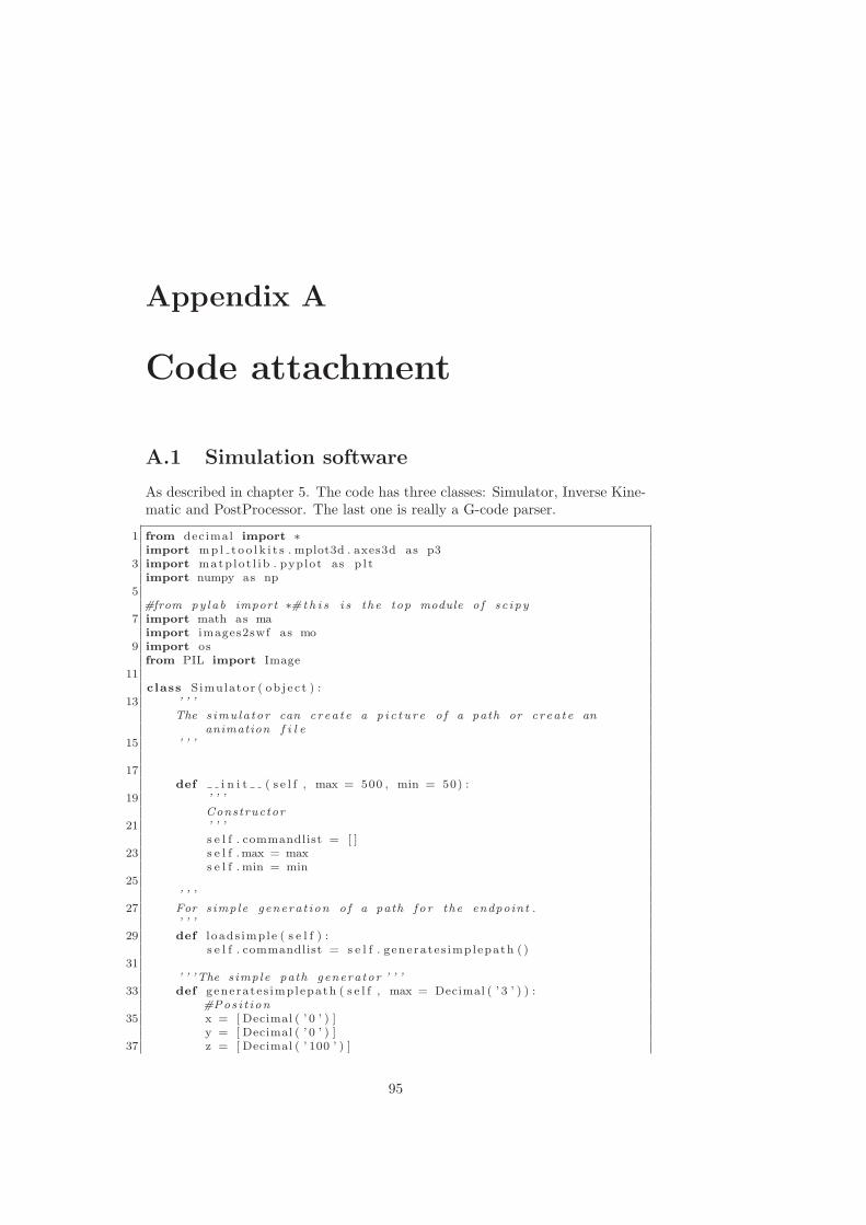
Appendix A

Code attachment

A.1 Simulation software

As described in chapter 5. The code has three classes: Simulator, Inverse Kine-matic and PostProcessor. The last one is really a G-code parser.

1 from decimal import ∗import mp l t o o l k i t s . mplot3d . axes3d as p3

3 import matp lo t l i b . pyplot as p l timport numpy as np

5#from py lab import ∗#t h i s i s the top module o f s c i py

7 import math as maimport images2swf as mo

9 import osfrom PIL import Image

11class Simulator ( ob j e c t ) :

13 ’ ’ ’The s imu la tor can crea t e a p i c t u r e o f a path or c rea t e an

animation f i l e15 ’ ’ ’

17def i n i t ( s e l f , max = 500 , min = 50) :

19 ’ ’ ’Constructor

21 ’ ’ ’s e l f . commandlist = [ ]

23 s e l f .max = maxs e l f . min = min

25’ ’ ’

27 For s imple genera t ion o f a path f o r the endpoint .’ ’ ’

29 def l oads imple ( s e l f ) :s e l f . commandlist = s e l f . generates implepath ( )

31’ ’ ’The s imple path generator ’ ’ ’

33 def generates implepath ( s e l f , max = Decimal ( ’ 3 ’ ) ) :#Pos i t ion

35 x = [ Decimal ( ’ 0 ’ ) ]y = [ Decimal ( ’ 0 ’ ) ]

37 z = [ Decimal ( ’ 100 ’ ) ]

95

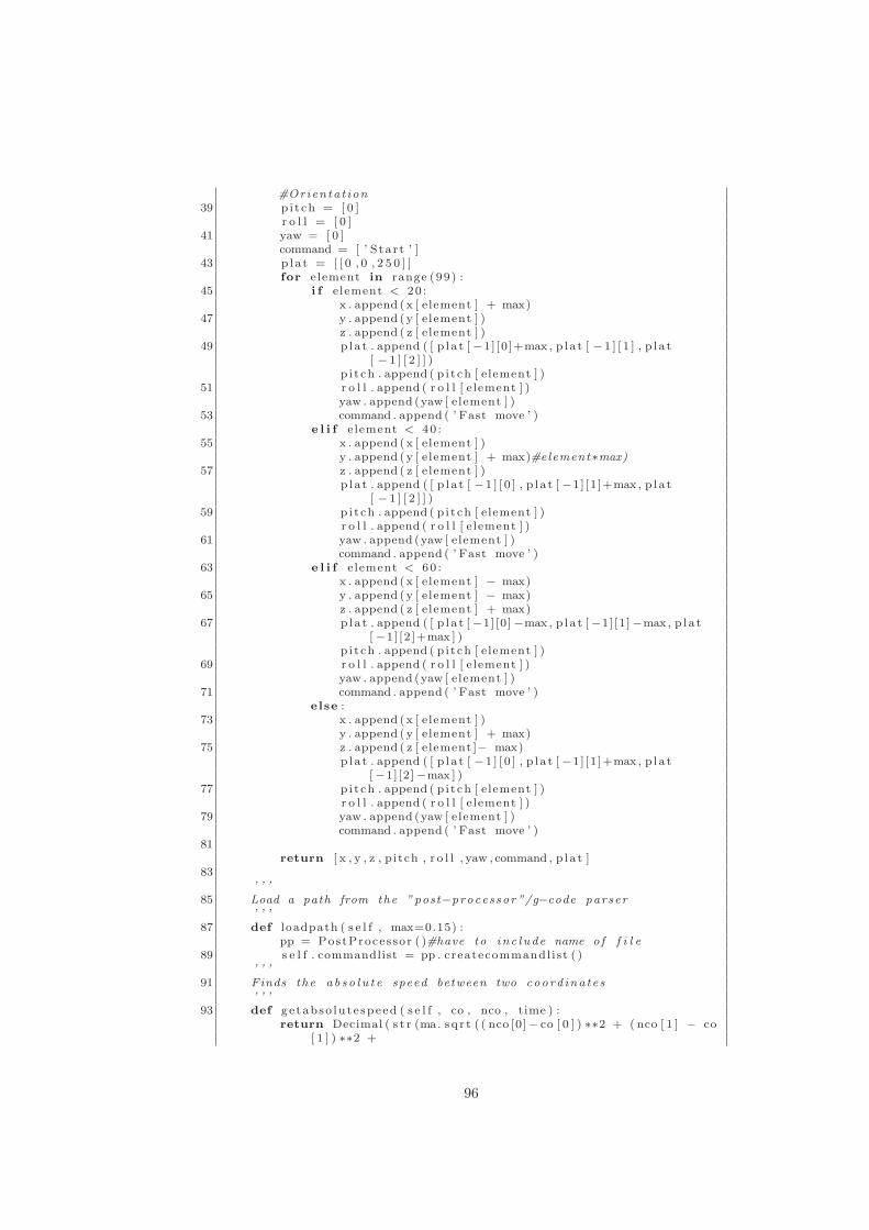
#Orienta t ion39 p i t ch = [ 0 ]

r o l l = [ 0 ]41 yaw = [ 0 ]

command = [ ’ S ta r t ’ ]43 p l a t = [ [ 0 , 0 , 2 5 0 ] ]

for element in range (99) :45 i f element < 20 :

x . append (x [ element ] + max)47 y . append (y [ element ] )

z . append ( z [ element ] )49 p l a t . append ( [ p l a t [−1] [0 ]+max , p l a t [ −1 ] [ 1 ] , p l a t

[ − 1 ] [ 2 ] ] )p i t ch . append ( p i t ch [ element ] )

51 r o l l . append ( r o l l [ e lement ] )yaw . append (yaw [ element ] )

53 command . append ( ’ Fast move ’ )e l i f element < 40 :

55 x . append (x [ element ] )y . append (y [ element ] + max)#element ∗max)

57 z . append ( z [ element ] )p l a t . append ( [ p l a t [ −1 ] [ 0 ] , p l a t [−1] [1 ]+max , p l a t

[ − 1 ] [ 2 ] ] )59 p i t ch . append ( p i t ch [ element ] )

r o l l . append ( r o l l [ e lement ] )61 yaw . append (yaw [ element ] )

command . append ( ’ Fast move ’ )63 e l i f element < 60 :

x . append (x [ element ] − max)65 y . append (y [ element ] − max)

z . append ( z [ element ] + max)67 p l a t . append ( [ p l a t [−1] [0]−max , p l a t [−1] [1]−max , p l a t

[−1] [2 ]+max ] )p i t ch . append ( p i t ch [ element ] )

69 r o l l . append ( r o l l [ e lement ] )yaw . append (yaw [ element ] )

71 command . append ( ’ Fast move ’ )else :

73 x . append (x [ element ] )y . append (y [ element ] + max)

75 z . append ( z [ element ]− max)p l a t . append ( [ p l a t [ −1 ] [ 0 ] , p l a t [−1] [1 ]+max , p l a t

[−1] [2]−max ] )77 p i t ch . append ( p i t ch [ element ] )

r o l l . append ( r o l l [ e lement ] )79 yaw . append (yaw [ element ] )

command . append ( ’ Fast move ’ )81

return [ x , y , z , p itch , r o l l , yaw , command , p l a t ]83

’ ’ ’85 Load a path from the ”post−processor ”/g−code parser

’ ’ ’87 def loadpath ( s e l f , max=0.15) :

pp = PostProcessor ( )#have to inc lude name of f i l e89 s e l f . commandlist = pp . createcommandl i st ( )

’ ’ ’91 Finds the a b s o l u t e speed between two coord ina te s

’ ’ ’93 def ge tabso lu t e speed ( s e l f , co , nco , time ) :

return Decimal ( s t r (ma. s q r t ( ( nco [0]− co [ 0 ] ) ∗∗2 + ( nco [ 1 ] − co[ 1 ] ) ∗∗2 +

96

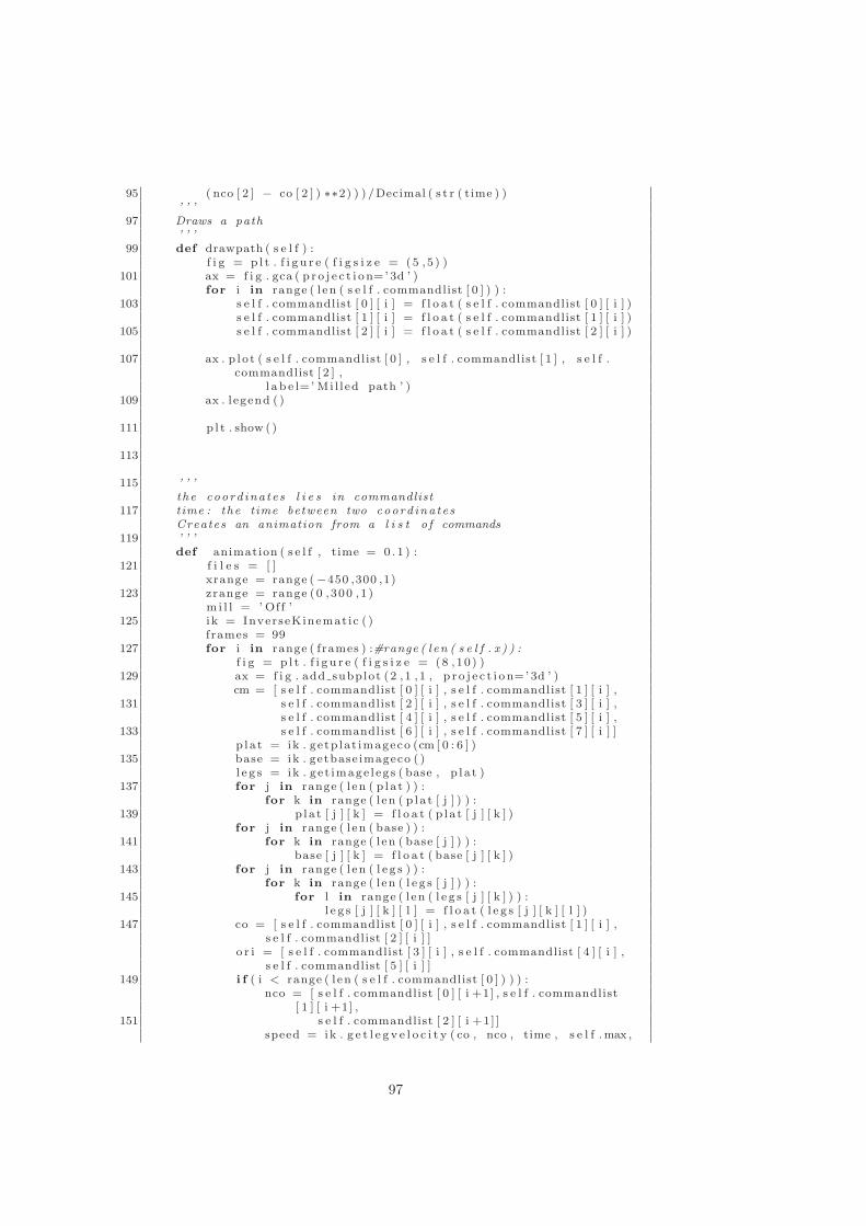
95 ( nco [ 2 ] − co [ 2 ] ) ∗∗2) ) ) /Decimal ( s t r ( time ) )’ ’ ’

97 Draws a path’ ’ ’

99 def drawpath ( s e l f ) :f i g = p l t . f i g u r e ( f i g s i z e = (5 , 5 ) )

101 ax = f i g . gca ( p r o j e c t i o n=’ 3d ’ )for i in range ( l en ( s e l f . commandlist [ 0 ] ) ) :

103 s e l f . commandlist [ 0 ] [ i ] = f l o a t ( s e l f . commandlist [ 0 ] [ i ] )s e l f . commandlist [ 1 ] [ i ] = f l o a t ( s e l f . commandlist [ 1 ] [ i ] )

105 s e l f . commandlist [ 2 ] [ i ] = f l o a t ( s e l f . commandlist [ 2 ] [ i ] )

107 ax . p l o t ( s e l f . commandlist [ 0 ] , s e l f . commandlist [ 1 ] , s e l f .commandlist [ 2 ] ,

l a b e l=’ Mi l l ed path ’ )109 ax . l egend ( )

111 p l t . show ( )

113

115 ’ ’ ’the coord ina te s l i e s in commandlist

117 time : the time between two coord ina te sCreates an animation from a l i s t o f commands

119 ’ ’ ’def animation ( s e l f , time = 0 . 1 ) :

121 f i l e s = [ ]xrange = range (−450 ,300 ,1)

123 zrange = range (0 ,300 ,1 )m i l l = ’ Off ’

125 ik = InverseKinemat ic ( )frames = 99

127 for i in range ( frames ) :#range ( l en ( s e l f . x ) ) :f i g = p l t . f i g u r e ( f i g s i z e = (8 ,10 ) )

129 ax = f i g . add subplot (2 , 1 , 1 , p r o j e c t i o n=’ 3d ’ )cm = [ s e l f . commandlist [ 0 ] [ i ] , s e l f . commandlist [ 1 ] [ i ] ,

131 s e l f . commandlist [ 2 ] [ i ] , s e l f . commandlist [ 3 ] [ i ] ,s e l f . commandlist [ 4 ] [ i ] , s e l f . commandlist [ 5 ] [ i ] ,

133 s e l f . commandlist [ 6 ] [ i ] , s e l f . commandlist [ 7 ] [ i ] ]p l a t = ik . getp lat imageco (cm [ 0 : 6 ] )

135 base = ik . getbase imageco ( )l e g s = ik . ge t image l eg s ( base , p l a t )

137 for j in range ( l en ( p l a t ) ) :for k in range ( l en ( p l a t [ j ] ) ) :

139 p l a t [ j ] [ k ] = f l o a t ( p l a t [ j ] [ k ] )for j in range ( l en ( base ) ) :

141 for k in range ( l en ( base [ j ] ) ) :base [ j ] [ k ] = f l o a t ( base [ j ] [ k ] )

143 for j in range ( l en ( l e g s ) ) :for k in range ( l en ( l e g s [ j ] ) ) :

145 for l in range ( l en ( l e g s [ j ] [ k ] ) ) :l e g s [ j ] [ k ] [ l ] = f l o a t ( l e g s [ j ] [ k ] [ l ] )

147 co = [ s e l f . commandlist [ 0 ] [ i ] , s e l f . commandlist [ 1 ] [ i ] ,s e l f . commandlist [ 2 ] [ i ] ]

o r i = [ s e l f . commandlist [ 3 ] [ i ] , s e l f . commandlist [ 4 ] [ i ] ,s e l f . commandlist [ 5 ] [ i ] ]

149 i f ( i < range ( l en ( s e l f . commandlist [ 0 ] ) ) ) :nco = [ s e l f . commandlist [ 0 ] [ i +1] , s e l f . commandlist

[ 1 ] [ i +1] ,151 s e l f . commandlist [ 2 ] [ i +1] ]

speed = ik . g e t l e g v e l o c i t y ( co , nco , time , s e l f .max ,

97

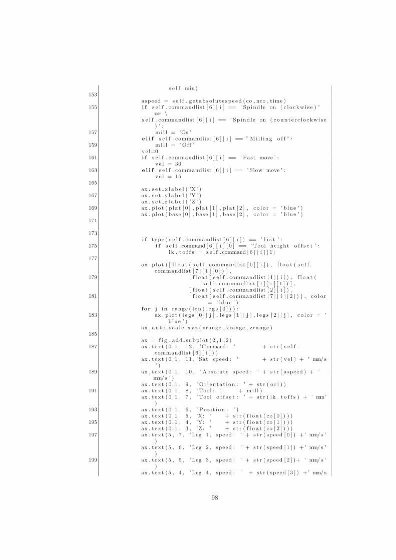
s e l f . min )153

aspeed = s e l f . g e tabso lu t e speed ( co , nco , time )155 i f s e l f . commandlist [ 6 ] [ i ] == ’ Sp ind le on ( c l o ckw i s e ) ’

or \s e l f . commandlist [ 6 ] [ i ] == ’ Sp ind le on ( counte r c l o ckw i s e

) ’ :157 m i l l = ’On ’

e l i f s e l f . commandlist [ 6 ] [ i ] == ”Mi l l i n g o f f ” :159 m i l l = ’ Off ’

v e l=0161 i f s e l f . commandlist [ 6 ] [ i ] == ’ Fast move ’ :

v e l = 30163 e l i f s e l f . commandlist [ 6 ] [ i ] == ’ Slow move ’ :

v e l = 15165

ax . s e t x l a b e l ( ’X ’ )167 ax . s e t y l a b e l ( ’Y ’ )

ax . s e t z l a b e l ( ’Z ’ )169 ax . p l o t ( p l a t [ 0 ] , p l a t [ 1 ] , p l a t [ 2 ] , c o l o r = ’ blue ’ )

ax . p l o t ( base [ 0 ] , base [ 1 ] , base [ 2 ] , c o l o r = ’ blue ’ )171

173i f type ( s e l f . commandlist [ 6 ] [ i ] ) == ’ l i s t ’ :

175 i f s e l f . command [ 6 ] [ i ] [ 0 ] == ’ Tool he ight o f f s e t ’ :i k . t o f f s = s e l f . command [ 6 ] [ i ] [ 1 ]

177ax . p l o t ( [ f l o a t ( s e l f . commandlist [ 0 ] [ i ] ) , f l o a t ( s e l f .

commandlist [ 7 ] [ i ] [ 0 ] ) ] ,179 [ f l o a t ( s e l f . commandlist [ 1 ] [ i ] ) , f l o a t (

s e l f . commandlist [ 7 ] [ i ] [ 1 ] ) ] ,[ f l o a t ( s e l f . commandlist [ 2 ] [ i ] ) ,

181 f l o a t ( s e l f . commandlist [ 7 ] [ i ] [ 2 ] ) ] , c o l o r= ’ blue ’ )

for j in range ( l en ( l e g s [ 0 ] ) ) :183 ax . p l o t ( l e g s [ 0 ] [ j ] , l e g s [ 1 ] [ j ] , l e g s [ 2 ] [ j ] , c o l o r = ’

blue ’ )ax . au t o s c a l e xy z ( xrange , xrange , zrange )

185ax = f i g . add subplot ( 2 , 1 , 2 )

187 ax . t ex t ( 0 . 1 , 12 , ’Command: ’ + s t r ( s e l f .commandlist [ 6 ] [ i ] ) )

ax . t ex t ( 0 . 1 , 11 , ’ Sat speed : ’ + s t r ( v e l ) + ’ mm/ s’ )

189 ax . t ex t ( 0 . 1 , 10 , ’ Absolute speed : ’ + s t r ( aspeed ) + ’mm/ s ’ )

ax . t ex t ( 0 . 1 , 9 , ’ Or i entat i on : ’ + s t r ( o r i ) )191 ax . t ex t ( 0 . 1 , 8 , ’ Tool : ’ + m i l l )

ax . t ex t ( 0 . 1 , 7 , ’ Tool o f f s e t : ’ + s t r ( i k . t o f f s ) + ’ mm’)

193 ax . t ex t ( 0 . 1 , 6 , ’ Po s i t i on : ’ )ax . t ex t ( 0 . 1 , 5 , ’X: ’ + s t r ( f l o a t ( co [ 0 ] ) ) )

195 ax . t ex t ( 0 . 1 , 4 , ’Y: ’ + s t r ( f l o a t ( co [ 1 ] ) ) )ax . t ex t ( 0 . 1 , 3 , ’Z : ’ + s t r ( f l o a t ( co [ 2 ] ) ) )

197 ax . t ex t (5 , 7 , ’ Leg 1 , speed : ’ + s t r ( speed [ 0 ] ) +’ mm/ s ’)

ax . t ex t (5 , 6 , ’ Leg 2 , speed : ’ + s t r ( speed [ 1 ] ) +’ mm/ s ’)

199 ax . t ex t (5 , 5 , ’ Leg 3 , speed : ’ + s t r ( speed [ 2 ] )+ ’ mm/ s ’)

ax . t ex t (5 , 4 , ’ Leg 4 , speed : ’ + s t r ( speed [ 3 ] ) +’ mm/ s

98

’ )201 ax . t ex t (5 , 3 , ’ Leg 5 , speed : ’ + s t r ( speed [ 4 ] ) +’ mm/ s

’ )ax . t ex t (5 , 2 , ’ Leg 6 , speed : ’ + s t r ( speed [ 5 ] )+ ’ mm/ s

’ )203 p l t . x t i c k s ( range (0 ,16 ,15 ) )

p l t . y t i c k s ( range (0 ,16 ,15 ) )205

fname = ’ tmp%03d . png ’%i207 f i g . s a v e f i g ( fname )

f i l e s . append ( Image . open ( fname ) )209 p l t . c l o s e ( ’ a l l ’ )

print i211 mo. writeSwf ( ’ t e s t . swf ’ , f i l e s )#can add durat ion o f each

image (1/ f p s ) to dec ide#fp s : d e f a u l t i s 0 .1

213 path = os . getcwd ( )for i in range ( frames ) :#range ( l en ( s e l f . x ) ) :

215 fname = ’ \ tmp%03d . png ’%if d e l = path + fname

217 os . remove ( f d e l )print ’Done ! ’

219

221 class InverseKinemat ic ( ob j e c t ) :’ ’ ’

223 A too l b o x f o r inve r s e k inemat ics’ ’ ’

225 def i n i t ( s e l f , t l eng th =150 , a=400 , c=250 ,b=400 ,d=250) :s e l f . a = a

227 s e l f . c = cs e l f . b = b

229 s e l f . d = ds e l f . t o f f s = 0

231 s e l f . t l eng th = t l eng th’ ’ ’

233 Returns the coord ina te s see from base’ ’ ’

235 def getcoord ( s e l f , co , pa r t z e ro ) :useco = co

237 useco [ 2 ] = useco [ 2 ]a1 = s e l f . ht ( useco )

239 a2 = s e l f . ht ( par t z e ro )m = np . dot ( a2 , a1 )#end−e f f e c t o r end seen from base

241 p l a t c en t e r = cop l a t c en t e r [ 2 ] = p l a t c en t e r [ 2 ] + s e l f . t l eng th + s e l f . t o f f s

243 a3 = s e l f . ht ( p l a t c en t e r )cfromb = np . dot ( a2 , a3 )#center o f p la t form seen from base

245

247 return [m[ 0 ] [ 3 ] , m[ 1 ] [ 3 ] , m[ 2 ] [ 3 ] ] , [ cfromb [ 0 ] [ 3 ] , cfromb[ 1 ] [ 3 ] , cfromb [ 2 ] [ 3 ] ]

249 ’ ’ ’Returns the center o f the p la t form ( g iven by l o c a l coord ina te s )

seen from base .251 ’ ’ ’

def ge tp l a t c en t e r f r ombaseco ( s e l f , co , m) :253 a1 = s e l f . ht ( co )

n i l = Decimal (0 )255 one = Decimal (1 )

a2 = [ [ one , n i l , n i l , n i l ] ,

99

257 [ n i l , one , n i l , n i l ] ,[ n i l , n i l , one , Decimal ( s t r ( s e l f . t l eng th ) ) ] ,

259 [ n i l , n i l , n i l , one ] ]t rans = np . dot ( a1 , a2 )

261 return [ t rans [ 0 ] [ 3 ] , t rans [ 1 ] [ 3 ] , t rans [ 2 ] [ 3 ] ]

263 ’ ’ ’From the t o o l t i p to the top p la t form

265 ’ ’ ’def htbasep la t ( s e l f , co ) :

267 a1 = s e l f . ht ( co )n i l = Decimal (0 )

269 one = Decimal (1 )a2 = [ [ one , n i l , n i l , n i l ] ,

271 [ n i l , one , n i l , n i l ] ,[ n i l , n i l , one , Decimal ( s t r ( s e l f . t l eng th ) ) ] ,

273 [ n i l , n i l , n i l , one ] ]

275 return np . dot ( a1 , a2 )

277 #the l o c a t i on o f the too l−t i p wi th o f f s e tdef g e t t o o l t i pwo f f c o ( s e l f , co ) :

279 a1 = s e l f . ht ( co )n i l = Decimal (0 )

281 one = Decimal (1 )a2 = [ [ one , n i l , n i l , n i l ] ,

283 [ n i l , one , n i l , n i l ] ,[ n i l , n i l , one , Decimal ( s t r (− s e l f . t o f f s ) ) ] ,

285 [ n i l , n i l , n i l , one ] ]t rans = np . dot ( a1 , a2 )

287 return [ t rans [ 0 ] [ 3 ] , t rans [ 1 ] [ 3 ] , t rans [ 2 ] [ 3 ] ]

289 ’ ’ ’Gets the l eng t h the l e g s have to move g iven two coord ina te s .

Intended to be used291 f o r programming the Arduino

’ ’ ’293 def g e t a r d l e g d i f f ( s e l f , co , nco , partzero , max , min ) :

#bs , coor = s e l f . ge tcoord ( co , par t z e ro )295 nowlegs = s e l f . g e t l e g l e n g t h s ( co )

bs , ncoor = s e l f . getcoord ( co , partzero , max , min )297 nex t l e g s = s e l f . g e t l e g l e n g t h s ( ncoor )

d i f f e r e n c e = [ ]299 a b s d i f f = [ ]

for i in range ( l en ( nowlegs ) ) :301 i f nowlegs [ i ] == False or nex t l e g s [ i ] == False :

return False , Fa l se303 for i in range ( l en ( nowlegs ) ) :

d i f f e r e n c e . append ( nex t l e g s [ i ] − nowlegs [ i ] )305 a b s d i f f . append (ma. sq r t ( d i f f e r e n c e [ i ]∗∗2 ) )

maxd i f f l e g = 0307 for i in range (1 , l en ( nowlegs ) ) :

i f a b s d i f f [ i ] > a b s d i f f [ maxd i f f l e g ] :309 maxd i f f l e g = i

return d i f f e r e n c e , maxd i f f l e g311

’ ’ ’313 Finds the v e l o c i t y f o r the l e g s

’ ’ ’315 def g e t l e g v e l o c i t y ( s e l f , co , nco , time , max , min ) :

#s e l f . s e t c oo rd ina t e s ( co )317 #next = InverseKinematic ( nco [ 0 ] , nco [ 1 ] , nco [ 2 ] , 0 , 0 , 0 )

100

l eg l engthsnow = s e l f . g e t l e g l e n g t h s ( co , max , min )#a l i s twi th s i x en t r i e s ,

319 #each entry has one va luel e g l e ng th sn ex t = s e l f . g e t l e g l e n g t h s ( nco , max , min )

321 speeds = [ ]for i in range (6 ) : #s i x l e g s

323 d i f f e r e n c e = l e g l eng th sn ex t [ i ] − l eg l engthsnow [ i ]speeds . append ( d i f f e r e n c e / time )

325 return speeds

327 ’ ’ ’Checks the v e l o c i t y f o r the l e g s

329 ’ ’ ’

331 def ch e ckv e l o c i t y ( s e l f , co , nco , maxdist , max , min ) :#s e l f . s e t c oo rd ina t e s ( co )

333 #next = InverseKinematic ( nco [ 0 ] , nco [ 1 ] , nco [ 2 ] , 0 , 0 , 0 )l eg l engthsnow = s e l f . g e t l e g l e n g t h s ( co , max , min )#a l i s t

wi th s i x en t r i e s ,335 #each entry has one va lue

l e g l e ng th sn ex t = s e l f . g e t l e g l e n g t h s ( nco , max , min )337 for i in range ( l en ( leg lengthsnow ) ) :

i f l eg l engthsnow [ i ] == False or l e g l e ng th sn ex t [ i ] ==False :

339 return Falsee r r o r = [ ]

341 for i in range (6 ) :d i f f e r e n c e = ma. sq r t ( ( l e g l eng th sn ex t [ i ] − l eg l engthsnow

[ i ] ) ∗∗2)343 i f d i f f e r e n c e > maxdist :

e r r o r . append ( i +1)345 i f l en ( e r r o r ) > 0 :

print ’ u i u i u i u i u i too f a s t ! ! ’347 return e r r o r

else :349 return [ 0 ]

#return speeds351

’ ’ ’353 This and ge tp la t imageco has the f i r s t l o c a t i on added to the

backReturns the po s i t i on o f the base (/ p la t form ) seen from the base

. In each s u b l i s t t he re355 are the x , y and z coord ina te s f o r the s i x l e g s .

’ ’ ’357 def getbase imageco ( s e l f ) :

Bx = [ Decimal ( s t r (ma. s q r t (3 ) /4∗ s e l f . b ) ) , Decimal ( s t r (−ma.sq r t (3 ) /4∗ s e l f . b ) ) ,

359 Decimal ( s t r (−ma. sq r t (3 ) /2∗( s e l f . b/2+ s e l f . d ) ) ) ,Decimal ( s t r (−ma. sq r t (3 ) /2∗( s e l f . b/2+ s e l f . d ) ) ) , Decimal

( s t r (−ma. sq r t (3 ) /4∗ s e l f . b ) ) ,361 Decimal ( s t r (ma. s q r t (3 ) /4∗ s e l f . b ) ) , Decimal ( s t r (ma. s q r t

(3 ) /4∗ s e l f . b ) ) ]By = [ Decimal ( s t r ( s e l f . d/2) ) , Decimal ( s t r ( ( s e l f . b+s e l f . d ) /2)

) , Decimal ( s t r ( s e l f . b/2) ) ,363 Decimal ( s t r (− s e l f . b/2) ) , Decimal ( s t r (−( s e l f . b+s e l f . d )

/2) ) , Decimal ( s t r (− s e l f . d/2) ) ,Decimal ( s t r ( s e l f . d/2) ) ]

365 Bz = [ 0 , 0 , 0 , 0 , 0 , 0 , 0 ]return [ Bx ,By , Bz ]

367’ ’ ’

101

369 Get the coord in s t e s f o r the p la t form to be used by drawn’ ’ ’

371 def getp lat imageco ( s e l f , co ) :p l a t co = s e l f . g e t p l a t j o i n t c o ( )

373 ht = s e l f . h tbasep la t ( co )imgco = [ [ ] , [ ] , [ ] ]

375#for each corner o f the p la t form

377 for element in p la t co :transpo = np . dot ( ht , element )

379 imgco [ 0 ] . append ( transpo [ 0 ] [ 0 ] )#ximgco [ 1 ] . append ( transpo [ 1 ] [ 0 ] )#y

381 imgco [ 2 ] . append ( transpo [ 2 ] [ 0 ] )#zimgco [ 0 ] . append ( imgco [ 0 ] [ 0 ] )

383 imgco [ 1 ] . append ( imgco [ 1 ] [ 0 ] )imgco [ 2 ] . append ( imgco [ 2 ] [ 0 ] )

385 return imgco’ ’ ’

387 Gives the l o c a t i on s o f the attachment po in t s from and fo r thecenter o f the base (/ p la t form )

389 ’ ’ ’def g e tba s e j o i n t c o ( s e l f ) :

391 B1 = [ [ma. s q r t (3 ) /4∗ s e l f . b ] , [ s e l f . d / 2 ] , [ 0 ] ]B2 = [[−ma. sq r t (3 ) /4∗ s e l f . b ] , [ ( s e l f . b+s e l f . d ) / 2 ] , [ 0 ] ]

393 B3 = [[−ma. sq r t (3 ) /2∗( s e l f . b/2+ s e l f . d ) ] , [ s e l f . b / 2 ] , [ 0 ] ]B4 = [[−ma. sq r t (3 ) /2∗( s e l f . b/2+ s e l f . d ) ] , [− s e l f . b / 2 ] , [ 0 ] ]

395 B5 = [[−ma. sq r t (3 ) /4∗ s e l f . b ] , [ − ( s e l f . b+s e l f . d ) / 2 ] , [ 0 ] ]B6 = [ [ma. s q r t (3 ) /4∗ s e l f . b ] , [− s e l f . d / 2 ] , [ 0 ] ]

397 return [ B1 ,B2 ,B3 ,B4 ,B5 ,B6 ]

399 def g e t l o c p l a t j o i n t c o ( s e l f ) :T1 = np . array ( [ [ma. s q r t (3 ) /2∗ s e l f . a / 2 ] , [ s e l f . a / 2 ] , [ 0 ] ] )

401 T2 = np . array ( [ [ma. s q r t (3 ) /2∗( s e l f . a/2− s e l f . c ) ] , [ ( s e l f . a+s e l f . c ) / 2 ] , [ 0 ] ] )

T3 = np . array ( [ [−ma. sq r t (3 ) /2∗( s e l f . a/2+ s e l f . c ) ] , [ s e l f . c/ 2 ] , [ 0 ] ] )

403 T4 = np . array ( [ [−ma. sq r t (3 ) /2∗( s e l f . a/2+ s e l f . c ) ] , [− s e l f . c/ 2 ] , [ 0 ] ] )

T5 = np . array ( [ [ma. s q r t (3 ) /2∗( s e l f . a/2− s e l f . c ) ] , [ − ( s e l f . a+s e l f . c ) / 2 ] , [ 0 ] ] )

405 T6 = np . array ( [ [ma. s q r t (3 ) /2∗ s e l f . a /2] , [− s e l f . a / 2 ] , [ 0 ] ] )return np . array ( [ T1 ,T2 ,T3 ,T4 ,T5 ,T6 ] )

407#Local coord ina te s o f the corners

409 def g e t p l a t j o i n t c o ( s e l f ) :T1 = [ [ Decimal ( s t r (ma. s q r t (3 ) /2∗ s e l f . a /2) ) ] , [ Decimal ( s t r (

s e l f . a /2) ) ] , [ 0 ] , [ 1 ] ]411 T2 = [ [ Decimal ( s t r (ma. s q r t (3 ) /2∗( s e l f . a/2− s e l f . c ) ) ) ] ,

[ Decimal ( s t r ( ( s e l f . a+s e l f . c ) /2) ) ] , [ 0 ] , [ 1 ] ]413 T3 = [ [ Decimal ( s t r (−ma. sq r t (3 ) /2∗( s e l f . a/2+ s e l f . c ) ) ) ] ,

[ Decimal ( s t r ( s e l f . c /2) ) ] , [ 0 ] , [ 1 ] ]415 T4 = [ [ Decimal ( s t r (−ma. sq r t (3 ) /2∗( s e l f . a/2+ s e l f . c ) ) ) ] ,

[ Decimal ( s t r (− s e l f . c /2) ) ] , [ 0 ] , [ 1 ] ]417 T5 = [ [ Decimal ( s t r (ma. s q r t (3 ) /2∗( s e l f . a/2− s e l f . c ) ) ) ] ,

[ Decimal ( s t r (−( s e l f . a+s e l f . c ) /2) ) ] , [ 0 ] , [ 1 ] ]419 T6 = [ [ Decimal ( s t r (ma. s q r t (3 ) /2∗ s e l f . a /2) ) ] , [ Decimal ( s t r (−

s e l f . a /2) ) ] , [ 0 ] , [ 1 ] ]return [ T1 ,T2 ,T3 ,T4 ,T5 ,T6 ]

421’ ’ ’

423 Coordinates f o r l e g s used in drawing images’ ’ ’

102

425 def ge t image l eg s ( s e l f , base=0, p l a t=0) :i f base ==0 or p la t ==0:

427 base = s e l f . getbase imageco ( )p l a t = s e l f . ge tp lat imageco ( )

429 image legs = [ [ ] , [ ] , [ ] ]for i in range (6 ) :

431 image legs [ 0 ] . append ( [ base [ 0 ] [ i ] , p l a t [ 0 ] [ i ] ] )image legs [ 1 ] . append ( [ base [ 1 ] [ i ] , p l a t [ 1 ] [ i ] ] )

433 image legs [ 2 ] . append ( [ base [ 2 ] [ i ] , p l a t [ 2 ] [ i ] ] )return image legs

435’ ’ ’

437 The l eng t h o f the l e g’ ’ ’

439 def g e t l e g l e n g t h s ( s e l f , co , max , min ) :base = s e l f . g e t b a s e j o i n t c o ( )

441 p l a t = s e l f . g e t p l a t j o i n t c o ( )l e g l e n g t h s = [ ]

443 for i in range ( l en ( base ) ) :l e g l e n g t h s . append ( s e l f . c a l c l e g l e n g t h s ( p l a t [ i ] , base [ i ] ,

co , max , min ) )445

return l e g l e n g t h s447 ’ ’ ’

Finds the l eng t h o f the l e g s449 ’ ’ ’

def c a l c l e g l e n g t h s ( s e l f , vectop , vecbase , co , max , min ) :451 homog = s e l f . ht ( [ co [ 0 ] , co [ 1 ] , co [ 2 ] , 0 , 0 , 0 ] )

for i in range ( l en ( vectop ) ) :453 vectop [ i ] = Decimal ( s t r ( vectop [ i ] [ 0 ] ) )

i f i < l en ( vecbase ) :455 vecbase [ i ] = Decimal ( s t r ( vecbase [ i ] [ 0 ] ) )

mid = np . dot (homog , vectop )457 #do t t = [ [ mid [ 0 ] ] , [ mid [ 1 ] ] , [ mid [ 2 ] ] ]

t = [ [ ] , [ ] , [ ] ]459 for i in range (3 ) :

t [ i ] = mid [ i ] − vecbase [ i ]461 l ength = ma. sq r t ( t [0 ]∗∗2+ t [1]∗∗2+ t [ 2 ] ∗ ∗ 2 )

i f l ength > max or l ength < min :463 print ’The l ength o f the l e g i s too smal l or too l a r g e !

Aborting . ’return False

465 else :return l ength

467#Homogenous trans format ion from pla t form to base

469 def ht ( s e l f , co ) :x = co [ 0 ]

471 y = co [ 1 ]z = co [ 2 ]

473 a = co [ 3 ]#alpha , beta , gammab = co [ 4 ]

475 g = co [ 5 ]n i l = Decimal (0 )

477 return [ [ Decimal ( s t r (ma. cos (b) ∗ma. cos ( g )+ma. s i n ( a ) ∗ma. s i n (b) ∗ma. s i n ( g ) ) ) ,

Decimal ( s t r (−ma. cos (b) ∗ma. s i n ( g )+ma. s i n ( a ) ∗ma. s i n (b) ∗ma. cos ( g ) ) ) ,

479 Decimal ( s t r (ma. cos ( a ) ∗ma. s i n (b) ) ) , Decimal ( s t r ( x ) )] ,

[ Decimal ( s t r (ma. cos ( a ) ∗ma. s i n ( g ) ) ) , Decimal ( s t r (ma.cos ( a ) ∗ma. cos ( g ) ) ) ,

103

481 Decimal ( s t r (−ma. s i n ( a ) ) ) , Decimal ( s t r ( y ) ) ] ,[ Decimal ( s t r (−ma. s i n (b) ∗ma. cos ( g )+ma. s i n ( a ) ∗ma. cos (

b) ∗ma. s i n ( g ) ) ) ,483 Decimal ( s t r (ma. s i n (b) ∗ma. s i n ( g ) + ma. s i n ( a ) ∗ma. cos

(b) ∗ma. cos ( g ) ) ) ,Decimal ( s t r (ma. cos ( a ) ∗ma. cos (b) ) ) , Decimal ( s t r ( z )

) ] ,485 [ n i l , n i l , n i l , Decimal (1 ) ] ]

487’ ’ ’

489 Notes :ONLY MILLING MODE HAS BEEN IMPLEMENTED NOT 3D PRINTING MODE

491 Output format i s what? A l i s t wi th p o s i t i o n s and o r i en t a t i on so f the endpoint wi th current speed .

493 ABC: or i en ta t i on , d e f a u l t s to degrees’ ’ ’

495 class PostProcessor ( ob j e c t ) :’ ’ ’

497 or G−code parser’ ’ ’

499 #type cou ld be ’ sim ’ ’ ard ’ or ’ d i s ’ ( d i s t ance c a l c u l a t i o ndef i n i t ( s e l f , pa r t z e ro = [0 , 0 , 100 , 0 , 0 , 0 ] , gcode=’M:/

gcode . txt ’ ,501 type = ’ sim ’ , time =0.1 , max = 500 , min = 50) :

s e l f . pa r t z e ro = par t ze ro#loca t i on o f ” par t zero ” the topand middle o f the

503 #part t ha t i s be ing mi l l e dgo = True

505 try :s e l f . gcode = open ( gcode , ’ r ’ )#Filename

507 except :print ’ Could not f i nd f i l e , e x i t i n g ’

509 go = Falsei f go == True :

511 s e l f . type = types e l f . speed = 1

513 s e l f . ab so lu t e = Trues e l f . run = True

515 s e l f . max = maxs e l f . min = min

517 s e l f . s k i p l i n e = Falses e l f . i k = InverseKinemat ic ( )

519 s e l f . l a s t p o s i t i o n = [ 0 , 0 , 0 , 0 , 0 , 0 ]s e l f . time = time #time in seconds between two en t r i e s

in the521 #commandlist f o r s imu la t ion time depends on f p s in the

#so f tware t ha t transforms p i c t u r e s in to a movie523 i f type == ’ sim ’ :

s t a r t , p l a t s t a r t = s e l f . i k . getcoord ( [ 0 , 0 , 0 , 0 , 0 , 0 ] ,s e l f . pa r t z e ro )

525 s e l f . commandlist = [ [ s t a r t [ 0 ] ] , [ s t a r t [ 1 ] ] , [ s t a r t[ 2 ] ] , [ 0 ] , [ 0 ] , [ 0 ] ,

[ ’ S ta r t ’ ] , [ p l a t s t a r t ] ]527 #Li s t to be returned to

s imu la tor#s e l f . createcommandl is t ( )

529 d = 0e l i f type == ’ ard ’ :

531 s e l f . commandlist = [ ]e l i f type == ’ d i s ’ :

533 s e l f . commandlist = [ ]

104

s e l f . f a s t d i s t = 0 .0535 s e l f . s l owd i s t = 0 .0

s e l f . m i l l d i s t = 0 .0537 s e l f . n onm i l l d i s t = 0 .0

s e l f . m i l l = Fal se539 #s e l f . createcommandl is t ( )

’ ’ ’541 Checks with the user whether he/ she wants to cont inue

’ ’ ’543 def checkcont inue ( s e l f ) :

answer = False545 while answer == False :

c = raw input ( ’> ’ ) ;547 i f c == ’y ’ or c == ’Y ’ :

answer = True549 e l i f c == ’n ’ or c == ’N ’ :

s e l f . run = False551 answer = True

’ ’ ’553 Creates a commandlist from the imported G−code f i l e .

A number o f commands are not implemented555 ’ ’ ’

def createcommandl i st ( s e l f ) :557 commands = s e l f . gcode . r e a d l i n e s ( )

move l i s t = [ False , False , False , False , False , Fa l se ]559 movenow = False

561 for i in range ( l en (commands) ) :i f l en ( s e l f . commandlist [ 0 ] ) > 200 :

563 break

s e l f . s k i p l i n e = False565 commandline = commands [ i ]

i f s e l f . run == True and ( commands [ i ] [ 0 ] == ’N ’ or

commands [ i ] [ 0 ] == ’n ’ ) :567 for j in range ( l en (commands [ i ] ) ) :

one = commands [ i ] [ j ]569 try :

one = in t ( one )571 except : pass

573 i f s e l f . s k i p l i n e == False and type ( one ) == s t rand one != ’ . ’ \

and one != ’N ’ :575 i f one == ’G’ or one == ’ g ’ :

s e l f . gcommand(commands [ i ] , j , i )577 e l i f one == ’M’ or one == ’m’ :

s e l f .mcommand(commands [ i ] , j , i )579 e l i f one == ’X ’ :

move l i s t [ 0 ] , movenow = s e l f . xyzabc (commands [ i ] , j , i )

581 e l i f one == ’Y ’ :move l i s t [ 1 ] , movenow = s e l f . xyzabc (

commands [ i ] , j , i )583 e l i f one == ’Z ’ :

move l i s t [ 2 ] , movenow = s e l f . xyzabc (commands [ i ] , j , i )

585 e l i f one == ’A ’ :move l i s t [ 3 ] , movenow = s e l f . xyzabc (

commands [ i ] , j , i )587 e l i f one == ’B ’ :

move l i s t [ 4 ] , movenow = s e l f . xyzabc (commands [ i ] , j , i )

105

589 e l i f one == ’C ’ :move l i s t [ 5 ] , movenow = s e l f . xyzabc (

commands [ i ] , j , i )591

e l i f one == ’F ’ :593 print ’Warning , command ’ , one , ’ in

l i n e ’ , i +1,’ could not be implemented . ’

595

597 i f l en (commands [ i ] )−1 == j and movenow ==True :movenow = False

599 now = [ s e l f . commandlist [ 0 ] [ −1 ] , s e l f .commandlist [ 1 ] [ −1 ] ,\

s e l f . commandlist [ 2 ] [ −1 ] , s e l f .commandlist [ 3 ] [ −1 ] ,\

601 s e l f . commandlist [ 4 ] [ −1 ] , s e l f .commandlist [ 5 ] [ − 1 ] ]

platnow = s e l f . commandlist [ 7 ] [ −1 ]603 for k in range ( l en ( move l i s t ) ) :

i f move l i s t [ k ] == False :605 move l i s t [ k ] = s e l f . l a s t p o s i t i o n

[ k ]i f s e l f . type == ’ sim ’ :

607 s e l f . addmovement (now , platnow , [Decimal ( s t r ( move l i s t [ 0 ] ) ) ,

Decimal ( s t r ( move l i s t [ 1 ] ) ) , Decimal (s t r ( move l i s t [ 2 ] ) ) ,

609 Decimal ( s t r ( move l i s t [ 3 ] ) ) , Decimal (s t r ( move l i s t [ 4 ] ) ) ,

Decimal ( s t r ( move l i s t [ 5 ] ) ) ] , s e l f .speed , s e l f . time )

611 e l i f s e l f . type == ’ ard ’ :s e l f . addardmove (now , platnow , [

Decimal ( s t r ( move l i s t [ 0 ] ) ) ,613 Decimal ( s t r ( move l i s t [ 1 ] ) ) , Decimal (

s t r ( move l i s t [ 2 ] ) ) ,Decimal ( s t r ( move l i s t [ 3 ] ) ) , Decimal (

s t r ( move l i s t [ 4 ] ) ) ,615 Decimal ( s t r ( move l i s t [ 5 ] ) ) ] , s e l f .

speed )e l i f s e l f . type == ’ d i s ’ :

617 s e l f . adddis tance ( s e l f . l a s t p o s i t i o n ,move l i s t )

s e l f . l a s t p o s i t i o n = move l i s t619 move l i s t = [ False , False , False , False ,

False , Fa l se ]return s e l f . commandlist

621’ ’ ’

623 Finds out what type o f G−command’ ’ ’

625 def gcommand( s e l f , commandline , j , i ) :i n f o l i s t = s e l f . getonetwothree ( commandline , j , i )

627 i f i n f o l i s t [ 1 ] != Fal se and i n f o l i s t [ 2 ] != Fal se :two = i n f o l i s t [ 1 ]

629 three = i n f o l i s t [ 2 ]i f two == ’ 0 ’ :

631 s e l f . gzero ( commandline , j , i , th r ee )e l i f two == ’ 2 ’ :

633 s e l f . gtwo ( commandline , j , i , th r ee )

106

e l i f two == ’ 4 ’ :635 s e l f . g four ( commandline , j , i , th r ee )

e l i f two == ’ 9 ’ :637 i f th ree == ’ 0 ’ :#abso l u t e programming

s e l f . ab so lu t e = True639 else :

print ’Warning , command G’ , two , three , ’could not be implemented . ’

641else :

643 print ’Warning , command G’ , two , three , ’ couldnot be implemented . ’

645 else :print ’Warning , command G in l i n e ’ , i +1, ’ could not

be implemented . ’647

’ ’ ’649 Finds what type o f G0x command

’ ’ ’651 def gzero ( s e l f , commandline , j , i , th r ee ) :

i f th ree == ’ 0 ’ :653 s e l f . speed = ’ f a s t ’

e l i f th ree == ’ 1 ’ :655 s e l f . speed = ’ slow ’

e l i f th ree == ’ 2 ’ or th ree == ’ 3 ’ :#Circu lar i n t e r p o l a t i o ni n t e r p o l a t i o n

657 print ’ C i r cu l a r i n t e r p o l a t i o n not implemented . Line ’ ,i +1, ’ w i l l be sk ipped . ’

s e l f . s k i p l i n e = True659 e l i f th ree == ’ 4 ’ :#dwe l l

try :661 i f commandline [ j +4] == ’P ’ or commandline [ j +4] == ’

U ’ or commandline [ j +4] == ’X ’ :dwel l t ime = 0

663 dwe l l s t r i n g = ’ ’for k in range ( j +4, l en ( commandline ) ) :

665 i f commandline [ k ] == ’ ’ :break

667 else :dwe l l s t r i n g = dwe l l s t r i n g + (

commandline [ k ] )669 dwel l t ime = in t ( dwe l l s t r i n g )

i f s e l f . type == ’ sim ’ :671 s e l f . add la s t ( )

for mm in range ( i n t ( dwel l t ime ) ∗10) :673 s e l f . commandlist [ 6 ] . append ( [ ’ Dwell f o r

some time ’ , dwel l t ime ] )e l i f s e l f . type == ’ ard ’ :

675 s e l f . commandlist . append ( [ 3 , dwel l t ime ] )except :

677 print ’Warning , could not implement dwel l in l i n e ’, i +1, ’ . ’

#pr in t ’ Could not implement dwe l l in l i n e ’ , i , ’ .Continue? [ y/n ] ’

679 #s e l f . checkcont inue ()else :

681 print ’Warning , could not implement G0 ’ , three , ’ . ’print ’Command, G0 ’ , three , ’ could not be implemented

, cont inue ? [ y/n ] ’683 s e l f . checkcont inue ( )

’ ’ ’

107

685 Finds type o f G2x command’ ’ ’

687 def gtwo ( s e l f , commandline , j , i , th r ee ) :i f th ree == ’ 0 ’ :#programming in inches

689 print ’ Inches as metr ic un i t not implemented . Terminate? [ y/n ] ’

print ’ I f no , the program w i l l use the va lue s asm i l l ime t e r s . ’

691 print ’ ( High r i s k o f crash e t c . ) ’s e l f . checkcont inue ( )

693 e l i f th ree == ’ 1 ’ :#programming in mi l l ime t e r si f s e l f . type == ’ sim ’ :

695 s e l f . add la s t ( )s e l f . commandlist [ 6 ] . append ( ’ Programming in

m i l l ime t e r s ’ )697 e l i f s e l f . type == ’ ard ’ :

s e l f . commandlist . append (0)699 e l i f th ree == ’ 8 ’ :#return to home po s i t i on

now = [ s e l f . commandlist [ −1 ] [ 0 ] ,701 s e l f . commandlist [ −1 ] [ 1 ] ,

s e l f . commandlist [ − 1 ] [ 2 ] ]703 i f s e l f . type == ’ sim ’ :

s e l f . addmovement (now , [ 0 , 0 , 0 ] , ’ f a s t ’ , s e l f . time )705 e l i f s e l f . type == ’ ard ’ :

s e l f . addardmovement (now , [ 0 , 0 , 0 ] , ’ f a s t ’ )707 else :

print ’Warning , command G2 ’ , three , ’ could not beimplemented . ’

709 #pr in t ’Command, G2 ’ , three , ’ cou ld not beimplemented , cont inue ? [ y/n ] ’

#s e l f . checkcont inue ()711

’ ’ ’713 Finds type o f G4x command

’ ’ ’715 def g four ( s e l f , commandline , j , i , th r ee ) :

hcheck = False717 try :

hcheck = commandline [ j +4]719 except : pass

i f hcheck != Fal se :721 i f th ree == ’ 3 ’ :#Tool h e i g h t o f f s e t compensation

nega t i v ei f hcheck == ’H ’ :#try

723 o f f s e t s t r i n g = ’ ’for k in range ( j +4, l en ( commandline ) ) :

725 i f commandline [ k ] == ’ ’ :break

727 else :o f f s e t s t r i n g = o f f s e t s t r i n g + (

commandline [ k ] )729 o f f s e t = − f l o a t ( o f f s e t s t r i n g )

s e l f . i k . s e t t o o l o f f s e t ( o f f s e t )731 i f s e l f . type == ’ sim ’ :

s e l f . add la s t ( )733 s e l f . commandlist [ 6 ] . append ( [ ’ Tool he ight

o f f s e t ’ , o f f s e t ] )e l i f s e l f . type == ’ ard ’ :

735 s e l f . commandlist . append ( [ 2 , o f f s e t ] )e l i f th ree == ’ 4 ’ :#Tool h e i g h t o f f s e t compensation

p o s i t i v e737 i f commandline [ j +4] == ’H ’ :#try

108

o f f s e t s t r i n g = ’ ’739 for k in range ( j +4, l en ( commandline ) ) :

i f commandline [ k ] == ’ ’ :741 break

else :743 o f f s e t s t r i n g = o f f s e t s t r i n g + (

commandline [ k ] )o f f s e t = f l o a t ( o f f s e t s t r i n g )

745 s e l f . i k . s e t t o o l o f f s e t ( o f f s e t )i f s e l f . type == ’ sim ’ :

747 s e l f . add la s t ( )s e l f . commandlist [ 6 ] . append ( [ ’ Tool he ight

o f f s e t ’ , o f f s e t ] )749 e l i f s e l f . type == ’ ard ’ :

s e l f . commandlist . append ( [ 2 , o f f s e t ] )751 e l i f th ree == ’ 9 ’ :#Tool l eng t h o f f s e t compensation

cance ls e l f . i k . s e t t o o l o f f s e t (0 )

753 i f s e l f . type == ’ sim ’ :s e l f . add la s t ( )

755 s e l f . commandlist [ 6 ] . append ( [ ’ Tool he ight o f f s e t’ , 0 ] )

e l i f s e l f . type == ’ ard ’ :757 s e l f . commandlist . append ( [ 2 , 0 ] )

else :759 print ’Warning , command G4 ’ , three , ’ could not be

implemented . ’else :

761 print ’Warning , command G4 ’ , three , ’ could not beimplemented . No value g iven ’

’ ’ ’763 Adds the pos i ton o f the l a s t command , used f o r non−moving

commands’ ’ ’

765 def add la s t ( s e l f ) :for i in range ( l en ( s e l f . commandlist ) ) :

767 i f i != 6 :s e l f . commandlist [ i ] . append ( s e l f . commandlist [ i ] [ −1 ] )

769 ’ ’ ’Decide type o f Mxx command

771 ’ ’ ’def mcommand( s e l f , commandline , j , i ) :

773 i n f o l i s t = s e l f . getonetwothree ( commandline , j , i )i f i n f o l i s t [ 1 ] != Fal se and i n f o l i s t [ 2 ] != Fal se :

775 two = i n f o l i s t [ 1 ]th ree = i n f o l i s t [ 2 ]

777 i f two == ’ 0 ’ :i f s e l f . type == ’ sim ’ :

779 i f th ree == ’ 0 ’ :#compulsory s tops e l f . add la s t ( )

781 s e l f . commandlist [ 6 ] . append ( ’ Stoppingmachine ! ’ )

s e l f . run =False783 e l i f th ree == ’ 1 ’ :#op t i ona l s top

s e l f . add la s t ( )785 s e l f . commandlist [ 6 ] . append ( ’Push button to

stop machine ! ’ )e l i f th ree == ’ 2 ’ :#end of program

787 s e l f . add la s t ( )s e l f . commandlist [ 6 ] . append ( ’End program ’ )

789 s e l f . run = Falsee l i f th ree == ’ 3 ’ :#sp ind l e on ( c l o c kw i s e )

109

791 s e l f . add la s t ( )s e l f . commandlist [ 6 ] . append ( ’ Sp ind le on (

c l o ckw i s e ) ’ )793 e l i f th ree == ’ 4 ’ :#sp ind l e on ( coun te rc l ockw i s e

)s e l f . add la s t ( )

795 s e l f . commandlist [ 6 ] . append ( ’ Sp ind le on (counte r c l o ckw i s e ) ’ )

e l i f th ree == ’ 5 ’ :#sp ind l e s top797 s e l f . add la s t ( )

s e l f . commandlist [ 6 ] . append ( ’ Stop sp i nd l e ’ )799 else :

print ’Warning , command , M’ , two , three ,801 ’ could not be implemented ’

e l i f s e l f . type == ’ ard ’ :803 i f th ree == ’ 0 ’ :#compulsory s top

s e l f . commandlist . append (1)805 e l i f th ree == ’ 1 ’ :#op t i ona l s top

s e l f . commandlist . append (2)807 e l i f th ree == ’ 2 ’ :#end of program

s e l f . commandlist . append (3)809 e l i f th ree == ’ 3 ’ :#sp ind l e on ( c l o c kw i s e )

s e l f . commandlist . append (4)811 e l i f th ree == ’ 4 ’ :#sp ind l e on ( coun te rc l ockw i s e

)s e l f . commandlist . append (5)

813 e l i f th ree == ’ 5 ’ :#sp ind l e s tops e l f . commandlist . append (6)

815 else :print ’Warning , command , M’ , two , three , \

817 ’ could not be implemented ’e l i f s e l f . type == ’ d i s ’ :

819 i f th ree == ’ 3 ’ or th ree == ’ 4 ’ :s e l f . m i l l = True

821 e l i f th ree == ’ 5 ’ :s e l f . m i l l = Fal se

823 else :print ’Waring , command , M’ , two , three , ’ could

not be implemented . ’825 #pr in t ’Command, M’ , two , three , ’ cou ld not be

implemented , cont inue ? [ y/n ] ’#s e l f . checkcont inue ()

827 ’ ’ ’Tries to f i nd the numbers a f t e r a command

829 ’ ’ ’def getonetwothree ( s e l f , commandline , j , i ) :

831 one = commandline [ j ]two = False

833 three = Falsetry :

835 two = commandline [ j +1]except :

837 print ’Warning , command ’ , one , ’ in l i n e ’ , i +1, ’could not be implemented . ’

i f two != False :839 try :

th r ee = commandline [ j +2]841 except :

print ’Warning , command ’ , one , two , ’ in l i n e ’ ,i +1,

843 ’ could not be implemented . ’

110

845 return [ one , two , th ree ]

847 ’ ’ ’Tries to f i nd x , y , z , a , b and c at the current l i n e f o r move

commands849 ’ ’ ’

def xyzabc ( s e l f , commandline , j , i ) :851 movenow = False

i f commandline [ j ] == ’X ’ :853 s e a r c h l i s t = [ ’Y ’ , ’Z ’ , ’A ’ , ’B ’ , ’C ’ ]

e l i f commandline [ j ] == ’Y ’ :855 s e a r c h l i s t = [ ’X ’ , ’Z ’ , ’A ’ , ’B ’ , ’C ’ ]

e l i f commandline [ j ] == ’Z ’ :857 s e a r c h l i s t = [ ’Y ’ , ’X ’ , ’A ’ , ’B ’ , ’C ’ ]

e l i f commandline [ j ] == ’A ’ :859 s e a r c h l i s t = [ ’Y ’ , ’Z ’ , ’X ’ , ’B ’ , ’C ’ ]

e l i f commandline [ j ] == ’B ’ :861 s e a r c h l i s t = [ ’Y ’ , ’Z ’ , ’A ’ , ’X ’ , ’C ’ ]

e l i f commandline [ j ] == ’C ’ :863 s e a r c h l i s t = [ ’Y ’ , ’Z ’ , ’A ’ , ’B ’ , ’X ’ ]

movestr ing = ’ ’865 for k in range ( j +1, l en ( commandline ) ) :

i f commandline [ k ] == ’ ’ or commandline [ k ] == ’ \n ’ :867 movenow = True

for m in range (k+1, l en ( commandline ) ) :869 i f commandline [m] in s e a r c h l i s t :

movenow = False871 break

break

873 else :movestr ing = movestr ing + commandline [ k ]

875 move = f l o a t ( movestr ing )return move , movenow

877 ’ ’ ’Add movement to be used to communicate with the Arduino

879 ’ ’ ’def addardmove ( s e l f , now , platnow , next , speed ) :

881 v = 1i f speed == ’ f a s t ’ :

883 v = 2e l i f speed == ’ slow ’ :

885 v = 1d i f f e r e n c e , max = s e l f . i k . g e t a r d l e g d i f f (now , next , s e l f .

partzero , s e l f .max ,887 s e l f . min )

i f d i f f e r e n c e == False :889 s e l f . run = False

else :891 s e l f . commandlist . append ( [ 1 , d i f f e r e n c e , max , v ] )

893 ’ ’ ’Add items to the commandlist l i s t g iven speed and s t a r t and end

po s i t i o n s895 Fast : 30 mm/s ( s u b j e c t to change )

Slow : 15 mm/s ( s u b j e c t to change )897 10 ’Hz ’ g i v e s 10 p i c t u r e s per second

s t a r t : the s t a r t i n g po in t o f the movement899 end : the ending po in t o f the movement

Fast : each p i c t u r e can move 0.30 mm901 Slow : each p i c t u r e can move 0.15 mm

’ ’ ’903 def addmovement ( s e l f , s t a r t , p l a t s t a r t , end , speed , s e c =0.1) :

111

v = 15905 i f speed == ’ f a s t ’ :

v = 30907 e l i f speed == ’ slow ’ :

v = 15909 pointend , p latend = s e l f . i k . getcoord ( end , s e l f . pa r t z e ro )

911 #Find the l e gn t h between the cen t r epo in t o f the p la t form atend and at s t a r t

l ength = Decimal ( s t r (ma. s q r t ( ( p latend [0]− p l a t s t a r t [ 0 ] ) ∗∗2 +( platend [ 1 ] −

913 p l a t s t a r t [ 1 ] ) ∗∗2 + ( platend [ 2 ] −p l a t s t a r t [ 2 ] ) ∗∗2) ) )

l e s s = v∗ s e c915 i f f l o a t ( l ength ) < l e s s :

print ’Too shor t between commands , w i l l use next , thel ength : ’ ,

917 f l o a t ( l ength )else :

919 l i s t e n t r i e s = in t (ma. c e i l ( l ength /Decimal ( s t r ( v∗ s e c ) ) ) )’ ’ ’ the sec at the end says how many

921 seconds between each command/ l i s t entry /framewhat i t does : f i n d s a b s o l u t e l eng t h between s t a r t and

end and d i v i d e s i t923 with the maximum l eng t h f o r the sa t speed and time

betweentwo en t r i e s . This equa l s the number o f e n t r i e s i s

needed between925 s t a r t and end with the g iven speed and time between two

en t r i e s .Ana lys i s i s f o r the endpoint . ’ ’ ’

927d e c l i s t = Decimal ( l i s t e n t r i e s ) #To use decimal to

perform mathematical opera t ions929 #pr in t ( end [0]− s t a r t [ 0 ] ) /0.3

xsteppo = Decimal ( s t r ( pointend [0]− s t a r t [ 0 ] ) ) / d e c l i s t931 ysteppo = Decimal ( s t r ( pointend [1]− s t a r t [ 1 ] ) ) / d e c l i s t

zsteppo = Decimal ( s t r ( pointend [2]− s t a r t [ 2 ] ) ) / d e c l i s t933

astep = Decimal ( s t r ( end [3]− s t a r t [ 3 ] ) ) / d e c l i s t935 bstep = Decimal ( s t r ( end [4]− s t a r t [ 4 ] ) ) / d e c l i s t

c s t ep = Decimal ( s t r ( end [5]− s t a r t [ 5 ] ) ) / d e c l i s t937

xs t epp l = Decimal ( s t r ( p latend [0]− p l a t s t a r t [ 0 ] ) ) / d e c l i s t939 ys t epp l = Decimal ( s t r ( p latend [1]− p l a t s t a r t [ 1 ] ) ) / d e c l i s t

z s t epp l = Decimal ( s t r ( p latend [2]− p l a t s t a r t [ 2 ] ) ) / d e c l i s t941

pos = s t a r t943 p la tpos = p l a t s t a r t

addangle = [ s t a r t [ 3 ] , s t a r t [ 4 ] , s t a r t [ 5 ] ]945 for i in range ( l i s t e n t r i e s ) :

pos = [ pos [0 ]+ xsteppo , pos [1 ]+ ysteppo , pos [2 ]+zsteppo ]

947 addangle = [ addangle [0 ]+ astep , addangle [1 ]+ bstep ,addangle [2 ]+ cs tep ]

p la tpos = [ p la tpos [0 ]+ xsteppl , p la tpos [1 ]+ ysteppl ,p la tpos [2 ]+ z s t epp l ]

949 p latnpos = [ p la tpos [0 ]+ xsteppl , p la tpos [1 ]+ ysteppl ,p la tpos [2 ]+ z s t epp l ]

addplatpos = s e l f . check l egspeed ( platpos , platnpos ,s e c ∗v )

951

112

i f l en ( addplatpos ) > 3 :953 d iv ided = len ( addplatpos ) /3

addpos =[ ]955 addangle = [ ]

newsteps = [ xsteppo / div ided , ysteppo / div ided ,zsteppo / d iv ided ]

957 newanglesteps = [ astep / div ided , bstep / div ided ,c s t ep / d iv ided ]

for j in range ( d iv ided ) :959 addpos . append ( newsteps [ 0 ] ∗ ( j +1) )

addpos . append ( newsteps [ 1 ] ∗ ( j +1) )961 addpos . append ( newsteps [ 2 ] ∗ ( j +1) )

addangle . append ( newanglesteps [ 0 ] ∗ ( j +1) )963 addangle . append ( newanglesteps [ 1 ] ∗ ( j +1) )

addangle . append ( newanglesteps [ 2 ] ∗ ( j +1) )965 else :

addpos = pos967

for j in range (0 , l en ( addpos ) ,3 ) :969 s e l f . commandlist [ 0 ] . append ( addpos [ j ] )

s e l f . commandlist [ 1 ] . append ( addpos [ j +1])971 s e l f . commandlist [ 2 ] . append ( addpos [ j +2])

s e l f . commandlist [ 3 ] . append ( addangle [ j ] )#i f noo r i en t a t i on i s g iven

973 s e l f . commandlist [ 4 ] . append ( addangle [ j +1])s e l f . commandlist [ 5 ] . append ( addangle [ j +2])

975 s e l f . commandlist [ 7 ] . append ( [ addplatpos [ j ] ,addplatpos [ j +1] ,

addplatpos [ j +2 ] ] )977 i f speed == ’ f a s t ’ :

s e l f . commandlist [ 6 ] . append ( ’ Fast move ’ )979 e l i f speed == ’ slow ’ :

s e l f . commandlist [ 6 ] . append ( ’ Slow move ’ )981

’ ’ ’983 Recursion :

Checks the speed o f the l e g s , i f the speed f o r one o f985 the l e g s i s too f a s t , the p o s i t i o n s are broken

up in two e t c . This func t i on /method i s f o r s imu la t ion .987 ’ ’ ’

def check l egspeed ( s e l f , pos , nextpos , maxdist ) :989 i f s e l f . run == True :

for i in range ( l en ( pos ) ) :991 pos [ i ] = Decimal ( pos [ i ] )

nextpos [ i ] = Decimal ( nextpos [ i ] )993 #0 success , 1−6 l e g t ha t f a i l e d

speedcheck = s e l f . i k . ch e ckv e l o c i t y ( pos , nextpos ,maxdist , s e l f .max ,

995 s e l f . min )returnpos = [ ]

997 i f speedcheck == False :s e l f . run == False

999 #return Falsee l i f 0 not in speedcheck :

1001 print ”Speed f o r l e g ( s ) ” , speedcheck ,” i s too f a s t . Movement i s s lowed down . ”

1003 #add a po in t in betweenmidpos = [ 0 , 0 , 0 ]

1005 for i in range ( l en ( nextpos ) ) :midpos [ i ] = Decimal ( s t r ( nextpos [ i ]−pos [ i ] ) )/2+

pos [ i ]1007 one = s e l f . check l egspeed ( pos , midpos , maxdist )

113

for i in range ( l en ( one ) ) :1009 returnpos . append ( one [ i ] )

one = s e l f . check l egspeed (midpos , nextpos , maxdist )1011 for i in range ( l en ( one ) ) :

r e turnpos . append ( one [ i ] )1013 return re turnpos

else :1015 returnpos = pos

return re turnpos1017 else :

return False1019

#Used fo r t e s t i n g :1021 pp = PostProcessor ( gcode=’ c : / gcode . txt ’ )

#com = pp . createcommandl is t ( )1023 sim = Simulator ( )

#sim . commandlist = com1025 sim . loads imple ( )

sim . animation ( )

Simulator.py

114

A.2 Biologically Inspired Path-optimization

This code is the implementation of what has been discussed in chapter 6. It has5 classes: GCodeReader, TestGA, GeneticAlgorithm, TestAnt and AntSystem.

#packeges used2 import math as ma

import numpy as np4 from decimal import ∗

import random6 import matp lo t l i b . pyplot as p l t

8class GcodeReader ( ob j e c t ) :

10 ’ ’ ’Parse G−code and the data to be used by the op t imi za t i on

12 a l gor i thms . Can a l s o f i nd l e n g t h s o f paths where the t o o li s i n a c t i v e ( f a s t ) ’ ’ ’

14 def i n i t ( s e l f , gcode=’M:/ gcode2 . txt ’ ) :’ ’ ’

16 Constructor’ ’ ’

18 go = Truetry :

20 s e l f . gcode = open ( gcode , ’ r ’ )#Filenameexcept :

22 print ’ Could not f i nd f i l e , e x i t i n g ’return False

24 go = Falsei f go == True :

26 s e l f . s l owd i s tance = 0s e l f . speed = False

28 s e l f . run = Trues e l f . s k i p l i n e = False

30 s e l f . l a s t p o s i t i o n = [ 0 , 0 , 0 ]s e l f . commandlist = [ ]

32 s e l f . f a s t d i s t = 0 .0s e l f . s l owd i s t = 0 .0

34 s e l f . m i l l d i s t = 0 .0s e l f . n onm i l l d i s t = 0 .0

36 s e l f . lastmovetype = Falses e l f . m i l l = Fal se

38 s e l f . t o o l o f f s e t = 0s e l f . f i r s t e l emen t = True

40 ’ ’ ’S t a r t to read the code , s im i l a r to ”Post processor ”/G−code

parser42 ’ ’ ’

def readgcode ( s e l f ) :44 commands = s e l f . gcode . r e a d l i n e s ( )

s e l f . move l i s t = [ False , False , Fa l se ]46 movenow = False

for i in range ( l en (commands) ) :48 s k i p l i n e = False

commandline = commands [ i ]50 s e l f . move l i s t = [ False , False , Fa l se ]

i f s e l f . run == True and ( commands [ i ] [ 0 ] == ’N ’ or

commands [ i ] [ 0 ] == ’n ’ ) :52 for j in range ( l en (commands [ i ] ) ) :

one = commands [ i ] [ j ]54 i f s k i p l i n e == False and type ( one ) == s t r and

one != ’ . ’ and one != ’N ’ :

115

i f one == ’G’ or one == ’ g ’ :56 i n f o l i s t = s e l f . getonetwothree (

commandline , j , i )i f i n f o l i s t [ 1 ] != Fal se and i n f o l i s t [ 2 ]

!= Fal se :58 two = i n f o l i s t [ 1 ]

th ree = i n f o l i s t [ 2 ]60 i f two == ’ 0 ’ :

i f th ree == ’ 0 ’ or th ree == ’ ’:

62 s e l f . speed = 2e l i f th ree == ’ 1 ’ :

64 s e l f . speed = 1e l i f th ree == ’ 2 ’ or th ree == ’

3 ’ :66 #c i r c u l a r i n t e r p o l a t i o n not

implementeds k i p l i n e = True

68 s e l f . speed = Falseprint ’ C i r cu l a r

i n t e r p o l a t i o n notimplemented , ’ ,

70 ’ sk ipp ing l i n e ’ , i+1e l i f two == ’ 1 ’ and th ree == ’ ’ :

72 s e l f . speed = 1e l i f two == ’ 2 ’ and th ree == ’ ’ :

74 s e l f . speed = Falses k i p l i n e = True

76 e l i f two == ’ 3 ’ and th ree == ’ ’ :s e l f . speed = False

78 s k i p l i n e = Truee l i f two == ’ 2 ’ and th ree == ’ 8 ’ :

80 s e l f . move l i s t = [ 0 , 0 , 0 ]s e l f . speed = 2

82 s e l f . movenow = Truee l i f two == ’ 4 ’ :#too l o f f s e t 43−

44+ 49 084 hcheck = False

try :86 hcheck = commandline [ j +4]

except : pass88

i f hcheck == ’H ’ :90 o f f s e t s t r i n g = ’ ’

for k in range ( j +4, l en (commandline ) ) :

92 i f commandline [ k ] == ’’ :break

94 else :o f f s e t s t r i n g =

o f f s e t s t r i n g +\

96 ( commandline [ k ] )i f th ree == ’ 3 ’ :#Tool

h e i g h t o f f s e t98 #compensation nega t i v e

s e l f . t o o l o f f s e t = −f l o a t ( o f f s e t s t r i n g )

100 e l i f th ree == ’ 4 ’ :#Toolh e i g h t o f f s e t#compensation p o s i t i v e

116

102 s e l f . t o o l o f f s e t = f l o a t( o f f s e t s t r i n g )

e l i f th ree == ’ 9 ’ :#Tooll eng t h o f f s e t

104 #compensation cance ls e l f . t o o l o f f s e t = 0

106 else :print ’Warning , command

G4 ’ , three ,108 ’ could not be

implemented . ’else :

110 print ’Warning , command G4 ’, three ,

’ could not be implemented .No value g iven ’

112 e l i f one == ’M’ or one == ’m’ :i n f o l i s t = s e l f . getonetwothree (

commandline , j , i )114 i f i n f o l i s t [ 1 ] != Fal se and i n f o l i s t [ 2 ]

!= Fal se :two = i n f o l i s t [ 1 ]

116 three = i n f o l i s t [ 2 ]i f two == ’ 0 ’ :

118 i f th ree == ’ 3 ’ or th ree == ’ 4 ’:s e l f . m i l l = True

120 e l i f th ree == ’ 5 ’ :s e l f . m i l l = Fal se

122 e l i f one == ’X ’ or one == ’x ’ :movenow = s e l f . f i ndva lu e (commands [ i ] , j

, ’X ’ )124 e l i f one == ’Y ’ or one == ’y ’ :

movenow = s e l f . f i ndva lu e (commands [ i ] , j, ’Y ’ )

126 e l i f one == ’Z ’ or one == ’ z ’ :movenow = s e l f . f i ndva lu e (commands [ i ] , j

, ’Z ’ )128 i f movenow == True :

i f s e l f . speed != Fal se :130 s e l f . addmovement ( )

movenow = False132 print s e l f . s l owd i s tance

’ ’ ’134 Finds the x , y and z va lue in a l i n e o f code

’ ’ ’136 def f i ndva lu e ( s e l f , l i n e , j , a x i s ) :

i f ax i s == ’X ’ :138 s e l f . move l i s t [ 0 ] = Decimal ( s t r ( s e l f . g e tva lue ( l i n e , j ) ) )

e l i f ax i s == ’Y ’ :140 s e l f . move l i s t [ 1 ] = Decimal ( s t r ( s e l f . g e tva lue ( l i n e , j ) ) )

e l i f ax i s == ’Z ’ :142 s e l f . move l i s t [ 2 ] = Decimal ( s t r ( s e l f . g e tva lue ( l i n e , j ) +

s e l f . t o o l o f f s e t ) )movenow = True

144for i in range ( j +1, l en ( l i n e ) ) :

146 i f l i n e [ i ] == ’X ’ or l i n e [ i ] == ’Y ’ or l i n e [ i ] == ’Z ’ :movenow = False

148 return movenow

150 ’ ’ ’

117

add movement informat ion to s e l f . commandlist152 ’ ’ ’

def addmovement ( s e l f ) :154 for i in range ( l en ( s e l f . move l i s t ) ) :

i f s e l f . move l i s t [ i ] == False :156 i f s e l f . f i r s t e l emen t == True :

s e l f . move l i s t [ i ] = 0158 else :

s e l f . move l i s t [ i ] = s e l f . commandlist [ − 1 ] [ 1 ] [ i ]160 i f s e l f . f i r s t e l emen t == True :

l a s t p o s = [ 0 , 0 , 0 ]162 s e l f . f i r s t e l emen t = False

else :164 l a s t p o s = s e l f . commandlist [ −1 ] [ 1 ]

d i s t anc e = Decimal ( s t r (ma. s q r t ( ( s e l f . move l i s t [0]− l a s t p o s[ 0 ] ) ∗∗2+

166 ( s e l f . move l i s t [1]− l a s t p o s [ 1 ] ) ∗∗2+( s e l f . move l i s t [2]− l a s t p o s [ 2 ] ) ∗∗2) ) )

168 i f s e l f . speed == 1 :s e l f . s l owd i s tance = s e l f . s l owd i s tance + d i s t anc e

170 i f s e l f . lastmovetype == s e l f . speed :#same type o f movements e l f . commandlist [ −1 ] [ 1 ] = s e l f . move l i s t [ : ]

172 s e l f . commandlist [ −1 ] [ 2 ] = s e l f . commandlist [ −1 ] [ 2 ] +d i s t anc e#increase d i s t ance

else :174 s e l f . commandlist . append ( [ l a s t p o s [ : ] , s e l f . move l i s t [ : ] ,

d i s tance , s e l f . speed ] )s e l f . lastmovetype = s e l f . speed

176’ ’ ’ Finds a number a f t e r a l e t t e r ’ ’ ’

178 def getva lue ( s e l f , l i n e , j ) :va lue = ’ ’

180 for i in range ( j +1, l en ( l i n e ) ) :i f l i n e [ i ] == ’ ’ :

182 break

else :184 value = value + l i n e [ i ]

debug = f l o a t ( va lue )186 print debug

return f l o a t ( va lue )188

’ ’ ’ Tries to f i nd the numbers a f t e r a command ’ ’ ’190 def getonetwothree ( s e l f , commandline , j , i ) :

one = commandline [ j ]192 two = False

three = False194 try :

two = commandline [ j +1]196 except :

print ’Warning , command ’ , one , ’ in l i n e ’ , i +1, ’could not be implemented . ’

198 i f two != False :try :

200 three = commandline [ j +2]except :

202 print ’Warning , command ’ , one , two , ’ in l i n e ’ ,i +1,

’ could not be implemented . ’204 return [ one , two , th ree ]

206 ’ ’ ’ Returns a l i s t o f a l l the s low movements ’ ’ ’def gets lowdata ( s e l f ) :

118

208 s l o w l i s t = [ ]s l o w l i s t . append ( [ [ 0 , 0 , 0 ] , [ 0 , 0 , 0 ] ] )

210 for i in range ( l en ( s e l f . commandlist ) ) :i f s e l f . commandlist [ i ] [ 3 ] == 1 :

212 s l o w l i s t . append ( s e l f . commandlist [ i ] [ 0 : 2 ] )return s l o w l i s t

214#crea t e s a l i s t o f d i s t ance s ( two between each entry ) and

re turns i t216 def p r epa r e f o r t sp ( s e l f , data ) :

d i s tancematr ix = [ [ 0 for x in data ] for x in data ]218 for i in range ( l en ( data ) ) :

for j in range ( i +1, l en ( data ) ) :220 #from s t a r t o f i to s t a r t o f j

d i s1 = ma. sq r t ( ( data [ i ] [ 0 ] [ 0 ] − data [ j ] [ 0 ] [ 0 ] ) ∗∗2+(data [ i ] [ 0 ] [ 1 ] − \

222 data [ j ] [ 0 ] [ 1 ] ) ∗∗2+(data [ i ] [ 0 ] [ 2 ] − data [ j] [ 0 ] [ 2 ] ) ∗∗2)

d i s 2 = ma. sq r t ( ( data [ i ] [ 1 ] [ 0 ] − data [ j ] [ 0 ] [ 0 ] ) ∗∗2+(data [ i ] [ 1 ] [ 1 ] − \

224 data [ j ] [ 0 ] [ 1 ] ) ∗∗2+(data [ i ] [ 1 ] [ 2 ] − data [ j] [ 0 ] [ 2 ] ) ∗∗2)

d i s 3 = ma. sq r t ( ( data [ i ] [ 0 ] [ 0 ] − data [ j ] [ 1 ] [ 0 ] ) ∗∗2+(data [ i ] [ 0 ] [ 1 ] − \

226 data [ j ] [ 1 ] [ 1 ] ) ∗∗2+(data [ i ] [ 0 ] [ 2 ] − data [ j] [ 1 ] [ 2 ] ) ∗∗2)

d i s 4 = ma. sq r t ( ( data [ i ] [ 1 ] [ 0 ] − data [ j ] [ 1 ] [ 0 ] ) ∗∗2+(data [ i ] [ 1 ] [ 1 ] − \

228 data [ j ] [ 1 ] [ 1 ] ) ∗∗2+(data [ i ] [ 1 ] [ 2 ] − data [ j] [ 1 ] [ 2 ] ) ∗∗2)

d i s tancematr ix [ i ] [ j ] = [ dis1 , d is2 , d is3 , d i s 4 ]230 d i s tancematr ix [ j ] [ i ] = [ dis1 , d is2 , d is3 , d i s 4 ]

return d i s tancematr ix232 ’ ’ ’ Returns the f a s t d i s t ance ’ ’ ’

def g e t f a s t d i s t a n c e ( s e l f , data ) :234 d i s t anc e = 0

for i in range (1 , l en ( data ) ) :236 d i s = ma. sq r t ( ( data [ i − 1 ] [ 1 ] [ 0 ] − data [ i − 1 ] [ 0 ] [ 0 ] ) ∗∗2+(

data [ i − 1 ] [ 1 ] [ 1 ] −data [ i − 1 ] [ 0 ] [ 1 ] ) ∗∗2 +(data [ i − 1 ] [ 1 ] [ 2 ] −

data [ i − 1 ] [ 0 ] [ 2 ] ) ∗∗2)238 d i s t anc e = d i s t anc e + d i s

d i s = ma. sq r t ( ( data [ − 1 ] [ 1 ] [ 0 ] − data [ 0 ] [ 0 ] [ 0 ] ) ∗∗2+(data[ − 1 ] [ 1 ] [ 1 ] − \

240 data [ 0 ] [ 0 ] [ 1 ] ) ∗∗2 +(data [ − 1 ] [ 1 ] [ 2 ] − data[ 0 ] [ 0 ] [ 2 ] ) ∗∗2)

d i s t anc e = d i s t anc e + d i s242 print ’ I n i t i a l d i s t anc e : ’ , d i s t anc e

return d i s t anc e244

’ ’ ’ Used f o r t e s t i n g the g ene t i c a lgor i thm ’ ’ ’246 class TestGA( ob j e c t ) :

def i n i t ( s e l f , runs , f i l e = ’ c : / gcode . txt ’ , p opu l a t i on s i z e= 100 ,

248 gene ra t i on s = 50 , pc = 0 . 6 , pm = 0 .1 , ranktype =1 , q = 0 . 5 ) :

o r i g i n a l l e n g t h = 0250 eva l s = 0

best = False252 worst = False

sumruns = 0254 ga = GeneticAlgorithm ( f i l e , popu la t i on s i z e , generat ions , pc

119

, pm, ranktype , q )o r i g i n a l l e n g t h = ga . g e t s t u f f ( )

256 for i in range ( runs ) :runbest = ga . master ( )

258 i f best == False :bes t = runbest [ : ]

260 else :i f runbest [ 0 ] < best [ 0 ] :

262 best = runbest [ : ]i f worst == False :

264 worst = runbest [ : ]else :

266 i f runbest [ 0 ] > worst [ 0 ] :worst = runbest [ : ]

268 eva l s = eva l s + ga . eva lua t i on ssumruns = sumruns + runbest [ 0 ]

270 meanbest = f l o a t ( sumruns ) / runspercentage = f l o a t ( bes t [ 0 ] ) / f l o a t ( o r i g i n a l l e n g t h ) ∗100

272 eva = eva l s / runsprint ’ Best ever : ’ , bes t [ 0 ]

274 print ’ Best run ever : ’ , bes t [ 1 : ]print ’ O r i g i na l l ength ’ , o r i g i n a l l e n g t h

276 print ’ Best ever percentage o f o r i g i n a l l ength ’ , percentageprint ’Worst ever : ’ , worst [ 0 ]

278 print ’Mean best f i t n e s s over ’ , runs , ’ runs : ’ , meanbestprint ’ Average number o f eva lua t i on s : ’ , eva

280’ ’ ’

282 Path−op t imi za t i on as TSP so l v ed by the g ene t i c a lgor i thmPMX crossover

284 Inver s ion mutationSUSampling

286 ranking s e l e c t i o ngene ra t i ona l replacement scheme with e l i t i sm

288 No of Generet ions terminat ion c r i t e r i o n

290 ’ ’ ’class GeneticAlgorithm ( ob j e c t ) :

292 def i n i t ( s e l f , f i l e = ’ c : / gcode ’ , p opu l a t i on s i z e = 100 ,g ene ra t i on s = 50 ,

pc = 0 . 6 , pm = 0 .1 , ranktype = 1 , q = 0 . 5 ) :294 s e l f . q = q

s e l f . f i l e = f i l e296 s e l f . e va l ua t i on s = 0 #number o f e va l ua t i on s

s e l f . ranktype = ranktype #1= expone t i a l , 0 = l i n e a r298 s e l f . pc = pc

s e l f .pm = pm300 i f popu l a t i on s i z e % 2 != 0 :

print ’ This a lgor i thm do not accept an odd number o f ’ ,302 ’ i n d i v i d u a l s in the populat ion . ’

print ’ Change to ’ , p opu l a t i on s i z e + 1 , ’ [ y ] or qu i t [ q] ? ’

304 popu l a t i on s i z e = popu l a t i on s i z e + 1#s e l f . o f f s p r i n g s i z e = o f f s p r i n g s i z e

306 s e l f . gener = gene ra t i on ss e l f . pops i z e = popu l a t i on s i z e

308 s e l f . popu lat ion = [ ]

310 ’ ’ ’ Get the data from the G−code reader ’ ’ ’def g e t s t u f f ( s e l f ) :

312 s e l f . gcr=0try :

120

314 s e l f . gcr = GcodeReader ( s e l f . f i l e )except :

316 pass

i f s e l f . gcr != Fal se :318 s e l f . gcr . readgcode ( )

s e l f . data = s e l f . gcr . gets lowdata ( )320 #s e l f . gcr . p r i n t f a s t d i s t a n c e ( s e l f . data )

s e l f . f i nd s l ow l eng th ( )322 s e l f . amount = len ( s e l f . data )#s i z e o f i n d i v i d u a l

s e l f . i n d i v i dua l = [ [ x ] for x in range ( s e l f . amount ) ]324 #di s tance matrix

s e l f . dismat = s e l f . gcr . p r epa r e f o r t sp ( s e l f . data )326 return s e l f . gcr . g e t f a s t d i s t a n c e ( s e l f . data )

328 ’ ’ ’ Get s imple data f o r i n i t i a l t e s t i n g ’ ’ ’def get s impledata ( s e l f ) :

330 s e l f . dismat = [ [ 0 for x in range (5 ) ] for x in range (5 ) ]s e l f . amount = len ( s e l f . dismat )

332 for i in range (1 , s e l f . amount ) :d i s 1 = random . rand int (0 ,100)

334 d i s 2 = random . rand int (0 ,100)s e l f . dismat [ 0 ] [ i ] = [ dis1 , d is1 , d is2 , d i s 2 ]

336 s e l f . dismat [ i ] [ 0 ] = [ dis1 , d is1 , d is2 , d i s 2 ]for i in range (1 , l en ( s e l f . dismat ) ) :

338 for j in range ( i , l en ( s e l f . dismat ) ) :i f i != j :

340 d i s t anc e = [ random . rand int (0 ,100) , random .rand int (0 ,100) ,

random . rand int (0 ,100) , random .rand int (0 ,100) ]

342 s e l f . dismat [ i ] [ j ] = d i s t anc es e l f . dismat [ j ] [ i ] = d i s t anc e

344 s e l f . i n d i v i dua l = [ [ x ] for x in range ( s e l f . amount ) ]

346 ’ ’ ’Main funct ion , c on t r o l s the o ther func t i ons ’ ’ ’def master ( s e l f ) :

348 s e l f . popu lat ion = [ ]s e l f . e va l ua t i on s = 0

350 s e l f . c r e a t e i n i t i a l ( )i t b e s t t o u r = [ ]

352 for i in range ( s e l f . gener ) :#i f b e s t i n d i v i d u a l = superbra : break

354 o f f s p r i n g = [ ]rankedind = s e l f . r ank ind i v i dua l s ( )

356 matingpool = s e l f . s e l e c t p a r e n t ( rankedind )for j in range (0 , s e l f . pops ize , 2 ) :

358 ch i l d 1 =[ ]ch i l d 2 =[ ]

360 parent1 =[ ]parent2 =[ ]

362 #Se l e c t parentsparent1 = matingpool . pop ( random . rand int (0 , s e l f .

pops ize−1− j ) )364 parent2 = matingpool . pop ( random . rand int (0 , s e l f .

pops ize−2− j ) )usepar1 = [ ]

366 usepar2 = [ ]for g f in range (1 , l en ( parent1 ) ) :

368 gene1 = [ ]gene2 = [ ]

370 for gg in range (2 ) :try :

121

372 gene1 . append ( parent1 [ g f ] [ gg ] )gene2 . append ( parent2 [ g f ] [ gg ] )

374 except :print ’ what now ’

376 usepar1 . append ( gene1 )usepar2 . append ( gene2 )

378 #Is there a cros sover ?p = random . uniform (0 , 1 )

380 i f p < s e l f . pc :ch i ld1 , ch i l d 2 = s e l f . c r o s s ov e r ( usepar1 , usepar2 )

382 #Is there a mutation o f the o f f s p r i n g ?p = random . uniform (0 , 1 )

384 i f p < s e l f .pm:ch i l d 1 = s e l f . mutate ( ch i l d 1 [ : ] )

386 ch i l d 2 = s e l f . mutate ( ch i l d 2 [ : ] )#Add the ch i l d r en with t h e i r tour l eng t h to the

o f f s p r i n g−poo l388 #ch i l d 1 . i n s e r t (0 , s e l f . e v a l u a t e i n d i v i d u a l (

c h i l d 1 ) )#ch i l d 2 . i n s e r t (0 , s e l f . e v a l u a t e i n d i v i d u a l (

c h i l d 2 ) )390 o f f s p r i n g . append ( ch i l d 1 [ : ] )

o f f s p r i n g . append ( ch i l d 2 [ : ] )392 else :

#i f no crossover , i s t he re a mutation o f theparents ?

394 p = random . uniform (0 , 1 )i f p < s e l f .pm:

396 mut1 = s e l f . mutate ( usepar1 )mut2 = s e l f . mutate ( usepar2 )

398 #Add the mutated parents wi th t h e i r l eng t hto the o f f s p r i n g−poo l

#mut1 . i n s e r t (0 , s e l f . e v a l u a t e i n d i v i d u a l (mut1) )

400 #mut2 . i n s e r t (0 , s e l f . e v a l u a t e i n d i v i d u a l (mut2) )

o f f s p r i n g . append (mut1 [ : ] )402 o f f s p r i n g . append (mut2 [ : ] )

else :404 #The parents surv i v ed f o r another

genera t ion !o f f s p r i n g . append ( parent1 [ : ] )

406 o f f s p r i n g . append ( parent2 [ : ] )

408 for o in range ( s e l f . pops i z e ) :i f type ( o f f s p r i n g [ o ] [ 0 ] )== l i s t :

410 jepp =[ ]for g f in range ( l en ( o f f s p r i n g [ o ] ) ) :

412 gene1 = [ ]

414 for gg in range (2 ) :try :

416 gene1 . append ( o f f s p r i n g [ o ] [ g f ] [ gg ] )

418 except :print ’ what now ’

420 jepp . append ( gene1 )tepp = s e l f . checkedges ( jepp )

422 co s t = s e l f . e v a l u a t e i nd i v i dua l ( tepp )ny = [ co s t ]

424 for p in tepp :ny . append (p)

122

426 o f f s p r i n g [ o ] = ny#Sort the o f f s p r i n g

428 o f f s p r i n g . s o r t ( )o f f s p r i n g [−1] = s e l f . popu lat ion [ 0 ] [ : ]#e l i t i sm

430 i t b e s t t o u r . append ( o f f s p r i n g [ − 1 ] [ 0 ] )#when genera t iona l , a l l o f f s p r i n g r ep l a ce the parents

432 s e l f . popu lat ion = [ ]s e l f . popu lat ion = o f f s p r i n g [ : ]

434 #Uncomment to a l l ow p l o t t i n g .’ ’ ’ ax = p l t . s u bp l o t (1 ,1 ,1)

436 x = range (0 , s e l f . gener )#x = range ( s e l f . ants )

438 #ax . p l o t ( x , l i s tmeantour , l a b e l = ”Mean”)ax . p l o t ( x , i t b e s t t o u r , l a b e l = ”Best in t h i s genera t ion ”)

440 p l t . y l a b e l ( ’ Cost o f tour ’ )p l t . g r i d (True )

442 #p l t . x l a b e l ( ’Ant ’ )p l t . x l a b e l ( ’ Generations ’ )

444 ax . l egend ( l o c=1, nco l=3, shadow=True )p l t . show () ’ ’ ’

446 co s t = s e l f . e v a l u a t e i nd i v i dua l ( s e l f . popu lat ion [ 0 ] [ 1 : ] )print s e l f . popu lat ion [ 0 ] [ 0 ]#sho r t e s t t r i p

448 #pr in t n r e va l #number o f e va l ua t i on s o f tourreturn s e l f . popu lat ion [ 0 ]

450’ ’ ’ Create i n i t i a l popu la t ion randomly ’ ’ ’

452 def c r e a t e i n i t i a l ( s e l f ) :for i in range ( s e l f . pops i z e ) :

454 ind = random . sample ( [ [ x ] for x in range ( s e l f . amount ) ] ,s e l f . amount )

i nd i v i dua l = s e l f . addrandomedges ( ind )456 i nd i v i dua l . i n s e r t (0 , s e l f . e v a l u a t e i nd i v i dua l ( i nd i v i dua l

) )s e l f . popu lat ion . append ( i nd i v i dua l )

458 s e l f . popu lat ion . s o r t ( )def addrandomedges ( s e l f , i n d i v i dua l ) :

460 for j in range ( l en ( i nd i v i dua l ) ) :i f j == 0 :

462 p = random . random ( )i f p <= 0 . 2 5 :

464 i nd i v i dua l [ j ] . append (0 )e l i f 0 .25 < p <= 0 . 5 :

466 i nd i v i dua l [ j ] . append (1 )e l i f 0 .5 < p <= 0 . 7 5 :

468 i nd i v i dua l [ j ] . append (2 )else :

470 i nd i v i dua l [ j ] . append (3 )else :

472 entry = ind i v i dua l [ j −1 ] [ 1 ]i f j == ( l en ( i nd i v i dua l )−1) :#l a s t element

474 in to = ind i v i dua l [ 0 ] [ 1 ]i f entry == 0 or entry == 2 :

476 i f i n t o == 0 or i n t o == 1 :i nd i v i dua l [ j ] . append (3 )

478 else :i n d i v i dua l [ j ] . append (2 )

480 else :i f i n t o == 0 or i n t o == 1 :

482 i nd i v i dua l [ j ] . append (1 )else :

484 i nd i v i dua l [ j ] . append (0 )else :

123

486 p = random . random ( )i f entry == 0 or entry == 2 :#enter s in 0

488 i f p <= 0 . 5 :i nd i v i dua l [ j ] . append (2 )

490 else :i n d i v i dua l [ j ] . append (3 )

492 e l i f entry == 1 or entry == 3 :#enter s in 1i f p <= 0 . 5 :

494 i nd i v i dua l [ j ] . append (0 )else :

496 i nd i v i dua l [ j ] . append (1 )i nd i v i dua l = s e l f . checkedges ( i nd i v i dua l )

498 return i n d i v i dua l

500 #Ranks the i n d i v i d u a l sdef r ank ind i v i dua l s ( s e l f ) :

502 #Total p ( percentage )totp = 0

504 #Sort the popu la t ion based on f i t n e s ss e l f . popu lat ion . s o r t ( )

506 ranked ind iv idua l s = [ ]

508 #Linear . For more d e t a i l s , see page 60−61 o f In t roduc t i onto

#Evo lu t ionary Computing ( Eiben and Smith 2007) .510 i f s e l f . ranktype == 0 :

s e l f . popu lat ion . r e v e r s e ( )#l e a s t f i t f i r s t512 #parameter i za t ion va lue 1.0 < s <= 2 . 0 :

s = 1 .5514 i = 0

for i n d i v i dua l in s e l f . popu lat ion :516 #Se l e c t i on p r o b a b i l i t y

#rever sed518 p s e l = (2− s ) / s e l f . pops i z e + 2∗ i ∗( s−1)/( s e l f . pops i z e

∗( s e l f . pops ize −1) )i += 1

520 #Should be 1 when f i n i s h e dtotp += ps e l

522 i f ( i <0) :print ’ Error ’

524 parent = [ i nd i v i dua l [ 0 ] , i n d i v i dua l [ 1 ] , pse l , totp ]r anked ind iv idua l s . append ( parent )

526 #Exponent ia l . For d e t a i l s , see (Michalewicz , 1994) or#h t t p ://www. aero . c a l t e c h . edu/˜ tamer/GATutorial . pdf

528 e l i f s e l f . ranktype == 1 :totp=1

530 q = s e l f . q #0.5for i in range ( s e l f . pops i z e ) :

532 pexp = q∗(1−q ) ∗∗( i ) #not rever sed popu la t ionparent = [ s e l f . popu lat ion [ i ] [ 0 ] ]

534 for j in range (1 , l en ( s e l f . popu lat ion [ i ] ) ) :parent . append ( s e l f . popu lat ion [ i ] [ j ] )

536 parent . append ( pexp )parent . append ( totp )

538 ranked ind iv idua l s . append ( parent )totp −= pexp

540 ranked ind iv idua l s . r e v e r s e ( )else :

542 print ’ e r ro r , wrong input f o r type o f ranking ’return r anked ind iv idua l s

544’ ’ ’ Eva luates an ind i v i dua l , f i n d s l eng t h o f path ’ ’ ’

124

546 def e v a l u a t e i nd i v i dua l ( s e l f , i n d i v i dua l ) :#The t o t a l number o f e va l ua t i on s

548 s e l f . e va l ua t i on s += 1f i t n e s s = 0

550 #Look through a l l the gene , add the cos t moving betweenthem

for i in range ( l en ( i nd i v i dua l ) ) :552 i f i != ( l en ( i nd i v i dua l )−1) :#not l a s t e lement

try :554 d i s t anc e = s e l f . dismat [ i nd i v i dua l [ i ] [ 0 ] ] [

i n d i v i dua l [ i + 1 ] [ 0 ] ] [ i n d i v i dua l [ i ] [ 1 ] ]except :

556 print ’ Something i s wrong with t h i s i nd i v i dua l ’

558 else : #l a s t element , move to f i r s td i s t anc e = s e l f . dismat [ i nd i v i dua l [ i ] [ 0 ] ] [ i n d i v i dua l

[ 0 ] [ 0 ] ] [ i n d i v i dua l [ i ] [ 1 ] ]560

f i t n e s s = f i t n e s s + d i s t anc e562 return f i t n e s s

564 ’ ’ ’ S e l e c t a parent based on ranking − SUS ’ ’ ’def s e l e c t p a r e n t ( s e l f , rankedind ) :

566 #current member : the po s i t i on in the mat ing poo l#i : the i n d i v i d u a l in the ranked par l i s t

568 currentmember = i = 0p = random . uniform (0 , 1 . 0/ l en ( rankedind ) )

570 #The poo l o f parentsmatingpool = [ ]

572 while ( currentmember < l en ( rankedind ) ) :while (p <= rankedind [ i ] [ −1 ] ) :

574 dork = rankedind [ i ] [ 0 : −2 ]matingpool . append ( dork [ : ] )

576 p = p + (1 . 0/ s e l f . pops i z e )currentmember = currentmember + 1

578 i = i + 1return matingpool

580’ ’ ’ Inver s ion mutation ’ ’ ’

582 def mutate ( s e l f , par ) :parent = par [ : ]

584 #The number o f genes to have t h e i r order inve r t edl ength = random . rand int (2 , l en ( parent )−2)

586 #The f i r s t gene to have i t s order inve r t edpo s i t i o n = random . rand int (0 , l en ( parent )−l ength )

588 ch i l d = parent [ : ]r e v e r s e db i t = parent [ p o s i t i o n : ( p o s i t i o n+length ) ] [ : ]

590 r e v e r s e db i t . r e v e r s e ( )for i in range ( l en ( r e v e r s e db i t ) ) :

592 ch i l d [ i+po s i t i o n ] = r e v e r s e db i t [ i ]#Fix the two broken l i n k s

594 #ch i l d = s e l f . addedges ( ch i l d , p o s i t i on )#ch i l d = s e l f . addedges ( ch i l d , p o s i t i on+leng th −1)

596 #ch i l d = s e l f . checkedges ( c h i l d [ : ] )#ch i l d = s e l f . c on t ro l ( ch i l d , True )

598 return ch i l d

600 ’ ’ ’ Check an i n d i v i d u a l f o r f a u l t s ’ ’ ’def c on t r o l ( s e l f , i nd i v idua l , mut) :

602 unused = s e l f . i n d i v i dua l [ : ]w rong l i s t = [ ]

604 for i in range ( l en ( i nd i v i dua l ) ) :

125

try :606 unused . remove ( [ i n d i v i dua l [ i ] [ 0 ] ] )

except :608 print ’Wrong with i nd i v i dua l ’

w rong l i s t . append ( i )610 for i in wrong l i s t :

i n d i v i dua l [ i ] = [ unused . pop ( ) , 0 ]612 s e l f . addedges ( i nd iv idua l , i )

i n d i v i dua l = s e l f . checkedges ( i nd i v i dua l )614 return i n d i v i dua l

616 ’ ’ ’PMX crossover by us ing two parents ’ ’ ’def c r o s s ov e r ( s e l f , par1 , par2 ) :

618 parent1 = par1 [ : ]parent2 = par2 [ : ]

620 #The number o f genes from parent 1 to be added to the c h i l dl ength = random . rand int (1 , l en ( s e l f . i n d i v i dua l )−2)

622 #The po s i t i on o f the f i r s t gene from parent 1try :

624 po s i t i o n = random . rand int (0 , l en ( parent1 )−l ength )except :

626 print ’ r ander ro r ’ch i l d 1 = [ Fa l se ]∗ l en ( parent1 )

628 ch i l d 2 = [ Fa l se ]∗ l en ( parent1 )map = [ [ ] , [ ] ]

630 #i = po s i t i on#Add genes from parent 1 to c h i l d 1 and genes from parent 2

to c h i l d 2632 for i in range ( po s i t i on , ( p o s i t i o n+length ) ) :

ch i l d 1 [ i ] = parent1 [ i ]634 ch i l d 2 [ i ] = parent2 [ i ]

map [ 0 ] . append ( parent1 [ i ] )636 map [ 1 ] . append ( parent2 [ i ] )

638 pos = po s i t i o n#Add genes from parent 2 to c h i l d 1 and from parent 1 to

c h i l d 2640 for i in range ( l en ( parent1 ) ) :

i f ch i l d 1 [ i ] == False :642 e x i s t = Fal se

for gene in ch i l d 1 [ p o s i t i o n : p o s i t i o n+length ] :644 i f gene [ 0 ] == parent2 [ i ] [ 0 ] :

e x i s t = True646 i f e x i s t == False :

ch i l d 1 [ i ] = parent2 [ i ]648 else :

c h i l d 1 [ i ] = s e l f . f i ndgene ( ch i ld1 , map , parent2 [i ] , 1)

650 e x i s t = Fal sefor gene in ch i l d 2 [ p o s i t i o n : p o s i t i o n+length ] :

652 i f gene [ 0 ] == parent1 [ i ] [ 0 ] :e x i s t = True

654 i f e x i s t == False :ch i l d 2 [ i ] = parent1 [ i ]

656 else :c h i l d 2 [ i ] = s e l f . f i ndgene ( ch i ld2 , map , parent1 [

i ] , 2)658

return ch i ld1 , ch i l d 2660

’ ’ ’ Check edges f o r co r r e c tne s s and f i x them ! ’ ’ ’662 def checkedges ( s e l f , i n d i v i dua l ) :

126

for i in range (1 , l en ( i nd i v i dua l ) ) :664 i f i == 0 :

be f o r e = ind i v i dua l [ −1 ] [ 1 ]666 else :

b e f o r e = ind i v i dua l [ i −1 ] [ 1 ]668 i f i == ( l en ( i nd i v i dua l )−1) :

next = ind i v i dua l [ 0 ] [ 1 ]670 else :

next = ind i v i dua l [ i +1 ] [ 1 ]672

i f be f o r e == 0 or be f o r e == 2 : #enter s at f ront , 0 and1 can not be used

674 i f next == 0 or next == 1 : #next use front , have touse 3

i n d i v i dua l [ i ] [ 1 ] = 3676 else : #have to use 2

i n d i v i dua l [ i ] [ 1 ] = 2678 else : #enter s at back , 2 and 3 cannot be used

i f next == 0 or next == 1 : #next use front , have touse 1−go in back

680 i nd i v i dua l [ i ] [ 1 ] = 1else :#have 0

682 i nd i v i dua l [ i ] [ 1 ] = 0return i n d i v i dua l

684’ ’ ’Add edges to an i n d i v i d u a l ’ ’ ’

686 def addedges ( s e l f , ch i ld , edge ) :i f edge >= ( len ( ch i l d )−1) :#end of i n d i v i d u a l

688 nextedge= ch i l d [ 0 ] [ 1 ]else :

690 try :nextedge = ch i l d [ edge +1 ] [ 1 ]

692 except :print ’wut? ’

694 i f edge == 0 :be fo reedge = ch i l d [ −1 ] [ 1 ]

696 else :b e fo r eedge = ch i l d [ edge −1 ] [ 1 ]

698 i f nextedge == 0 or nextedge == 1 :#can not use 0 or 2i f be fo reedge == 0 or be fo reedge == 2 :#can not use 0 or

1700 ch i l d [ edge ] [ 1 ] = 3

e l i f be fo reedge == 1 or be fo reedge == 3 :#can not use 2or 3

702 ch i l d [ edge ] [ 1 ] = 1e l i f nextedge == 2 or nextedge == 3 :#can not use 1 or 3

704 i f be fo reedge == 0 or be fo reedge == 2 :#can not use 0 or1ch i l d [ edge ] [ 1 ] = 2

706 e l i f be fo reedge == 1 or be fo reedge == 3 :#can not use 2or 3ch i l d [ edge ] [ 1 ] = 0

708 return ch i l d

710 ’ ’ ’ Used f o r PMX crossover , f i n d s the r i g h t gene ’ ’ ’def f i ndgene ( s e l f , ch i ld , map , gene , chnr ) :

712 index = 0for i in range ( l en (map [ chnr −1]) ) :

714 i f map [ chnr −1] [ i ] [ 0 ] == gene [ 0 ] :index = i

716 i f chnr == 1 :ok = True

127

718 for i in range ( l en ( ch i l d ) ) :i f type ( ch i l d [ i ] ) == l i s t :

720 i f ch i l d [ i ] [ 0 ] == map [ 1 ] [ index ] [ 0 ] :ok = False

722 i f ok == True :return map [ 1 ] [ index ]

724 else :return s e l f . f i ndgene ( ch i ld , map , map [ 1 ] [ index ] ,

chnr )726 e l i f chnr == 2 :

ok = True728 for i in range ( l en ( ch i l d ) ) :

i f type ( ch i l d [ i ] ) == l i s t :730 i f ch i l d [ i ] [ 0 ] == map [ 0 ] [ index ] [ 0 ] :

ok = False732 i f ok == True :

return map [ 0 ] [ index ]734 else :

return s e l f . f i ndgene ( ch i ld , map , map [ 0 ] [ index ] ,chnr )

736’ ’ ’ Used f o r t e s t i n g AntSystem ’ ’ ’

738 class TestAnt ( ob j e c t ) :def i n i t ( s e l f , runs , f i l e = ’m:/25D. txt ’ , ants = 10 , alpha

= 1 . 0 , beta = 1 . 0 ,740 Q = 1 .0 , rho = 0 . 7 , g ene ra t i on s = 50) :

o r i g i n a l l e n g t h = 0742 best = False

worst = False744 sumruns = 0

acs = AntSystem ( f i l e , ants , alpha , beta , Q, rho ,g ene ra t i on s )

746 o r i g i n a l l e n g t h = acs . g e t s t u f f ( )for i in range ( runs ) :

748 acs . addpheromone ( )runbest = acs . s t a r t ( )

750 i f best == False :bes t = runbest [ : ]

752 else :i f runbest [ 0 ] < best [ 0 ] :

754 best = runbest [ : ]i f worst == False :

756 worst = runbest [ : ]else :

758 i f runbest [ 0 ] > worst [ 0 ] :worst = runbest [ : ]

760 eva l s = acs . e va lua t i on ssumruns = sumruns + runbest [ 0 ]

762 meanbest = f l o a t ( sumruns ) / runspercentage = f l o a t ( bes t [ 0 ] ) / f l o a t ( o r i g i n a l l e n g t h ) ∗100

764 print ’ Best ever : ’ , bes t [ 0 ]print ’ Path : ’ , bes t [ 1 : ]

766 print ’ O r i g i na l l ength ’ , o r i g i n a l l e n g t hprint ’ Best ever percentage o f o r i g i n a l l ength ’ , percentage

768 print ’Worst ever : ’ , worst [ 0 ]print ’Mean best f i t n e s s over ’ , runs , ’ runs : ’ , meanbest

770 print ’ Average number o f eva lua t i on s : ’ , e v a l s

772 ’ ’ ’ So lve the TSP problem with Ant System ’ ’ ’class AntSystem ( ob j e c t ) :

774 def i n i t ( s e l f , f i l e = ’m:/ gcode2 . txt ’ , ants = 10 , alpha =1 . 0 , beta = 1 . 0 ,

128

Q = 1 .0 , rho = 0 . 7 , g ene ra t i on s = 50) :776 s e l f .Q = Q#constant : de l t a−tau=Q/ l eng t h

s e l f . rho = rho#evaporat ion ra t e778 s e l f . ants = ants

s e l f . alpha = alpha780 s e l f . beta = beta

s e l f . f i l e = f i l e782 s e l f . g ene ra t i on s = gene ra t i on s

s e l f . e va l ua t i on s = ants ∗ gene ra t i on s784

’ ’ ’ Get data from Gcode reader ’ ’ ’786 def g e t s t u f f ( s e l f ) :

s e l f . gcr=False788 try :

s e l f . gcr = GcodeReader ( s e l f . f i l e )790 #s e l f . gcr = True

except :792 print ’ Could not r e t r i e v e data ’

i f s e l f . gcr != Fal se :794 s e l f . gcr . readgcode ( )

s e l f . data = s e l f . gcr . gets lowdata ( )796 #s e l f . gcr . p r i n t f a s t d i s t a n c e ( s e l f . data )

s e l f . amount = len ( s e l f . data )#s i z e o f i n d i v i d u a l798 s e l f . i n d i v i dua l = [ [ x ] for x in range ( s e l f . amount ) ]

#di s tance matrix800 s e l f . dismat = s e l f . gcr . p r epa r e f o r t sp ( s e l f . data )

return s e l f . gcr . g e t f a s t d i s t a n c e ( s e l f . data )802

’ ’ ’ Get s imple data f o r t e s t i n g ’ ’ ’804 def get s impledata ( s e l f ) :

s e l f . dismat = [ [ 0 for x in range (5 ) ] for x in range (5 ) ]806 s e l f . amount = len ( s e l f . dismat )#leng t h o f i n d i v i d u a l

for i in range (1 , s e l f . amount ) :808 d i s 1 = random . rand int (0 ,100)

d i s 2 = random . rand int (0 ,100)810 s e l f . dismat [ 0 ] [ i ] = [ dis1 , d is1 , d is2 , d i s 2 ]

s e l f . dismat [ i ] [ 0 ] = [ dis1 , d is1 , d is2 , d i s 2 ]812 for i in range (1 , l en ( s e l f . dismat ) ) :

for j in range ( i , l en ( s e l f . dismat ) ) :814 i f i != j :

d i s t anc e = [ random . rand int (0 ,100) , random .rand int (0 ,100) ,

816 random . rand int (0 ,100) , random .rand int (0 ,100) ]

s e l f . dismat [ i ] [ j ] = d i s t anc e [ : ]818 s e l f . dismat [ j ] [ i ] = d i s t anc e [ : ]

820’ ’ ’Runs the a lgori thm , runs f o r a number o f genera t ions and

f i nd s the t o t a l822 b e s t run . ’ ’ ’

def s t a r t ( s e l f ) :824 #Average

l i s tmeantour = [ ]826 #Best f o r one run ( i t e r a t i o n b e s t tour )

i t b e s t t o u r = [ ]828 #Total s h o r t e s t tour ( b e s t so f a r )

s f b e s t t o u r = [ 0 ]830 #Add i n i t i a l pheromone concentra t ion i f nonex i s t en t .

i f type ( s e l f . dismat [ 0 ] [ 1 ] [ 0 ] ) != l i s t :832 s e l f . addpheromone ( )

te rminat ion = 0

129

834 s e l f . numbind = len ( s e l f . dismat [ 0 ] )#the number o f genesgene ra t i on s = 0

836 #Run a lgor i thmwhile te rminat ion == 0 :

838 gene ra t i on s += 1r o u t e l i s t = [ ] #l i s t conta in ing the route o f a l l the

ants o f t h i s genera t ion840 meantour = 0

bes t tour = 0842 for ant in range (0 , s e l f . ants ) :

l ength = 0844 s t a r t g ene = random . rand int (0 , s e l f . numbind−1)

t a b u l i s t =[ s t a r t g ene ] #the cu t s the ant has v i s i t e d846 unv i s i t ed = range (0 , s e l f . numbind ) #the cu t s the

ant has not ye t v i s i t e dtry :

848 unv i s i t ed . remove ( s t a r t g ene )except :

850 print ’ Could not remove ’ , s t a r t g ene , ’ fromunv i s i t ed i n d i v i d u a l s . ’

#Add the r e s t o f the cu t s852 for i in range (0 , s e l f . numbind−1) :

next , edge = s e l f . choosenext ( t abu l i s t , unv i s i t ed)

854 t a b u l i s t [−1] = [ t a b u l i s t [−1] , edge ]l ength = length + s e l f . dismat [ t a b u l i s t [ − 1 ] [ 0 ] ] [

next ] [ edge ] [ 0 ]856 t a b u l i s t . append ( next )

try :858 unv i s i t ed . remove ( next )

except :860 print ’ Something i s wrong with the program ’

#Add l eng t h from l a s t to f i r s t c i t y , complet ing thetour

862 s e l f . add las tedge ( t a b u l i s t )l ength += s e l f . dismat [ t a b u l i s t [ − 1 ] [ 0 ] ] [ t a b u l i s t

[ 0 ] [ 0 ] ] [ t a b u l i s t [ − 1 ] [ 1 ] ] [ 0 ]864 t a b u l i s t . append ( l ength )

meantour += length866

i f l ength < bes t tour or bes t tour == 0 :868 be s t tour = length

i f l ength < s f b e s t t o u r [ 0 ] or s f b e s t t o u r [ 0 ] == 0 :870 s f b e s t t o u r = [ length , t a b u l i s t [ : ] ]

s f b e s t t o u r [ 1 ] . pop ( )#??872 r o u t e l i s t . append ( t a b u l i s t )

874 #Updatemeantour = meantour/ s e l f . ants

876 l i s tmeantour . append (meantour )i t b e s t t o u r . append ( be s t tour )

878 s e l f . updatepheromonevalues ( r o u t e l i s t )

880 #the terminat ion cond i t i on i s :i f gene ra t i on s == s e l f . g ene ra t i on s :

882 #Uncomment to a l l ow p l o t t i n g .#ax = p l t . s u bp l o t (1 ,1 ,1)

884 #x = range (0 , genera t ions )#x = range ( s e l f . ants )

886 #ax . p l o t ( x , l i s tmeantour , l a b e l = ”Mean”)#ax . p l o t ( x , i t b e s t t o u r , l a b e l = ”Best ”)

888 #ax . p l o t ( x , r o u t e l i s t [ : ] [ −1 ] )

130

#p l t . y l a b e l ( ’ Cost o f tour ’ )890 #p l t . g r i d (True )

#p l t . x l a b e l ( ’Ant ’ )892 #p l t . x l a b e l ( ’ Generations ’ )

#ax . l egend ( l o c=1, nco l=3, shadow=True )894 #p l t . show ()

#pr in t ’The b e s t tour t rave r s ed : ’ , s f b e s t t o u r896 #f i n a l c i t y o r d e r = f i n a l r un ( s e l f . dismat , s e l f .

alpha , s e l f . be ta )#pr in t ’The l a s t run g i v e s a tour o f : ’ ,

f i n a l c i t y o r d e r898 #pr in t ’ ( Obvious ly the l a r g e number i s the l eng t h ) ’

te rminat ion = 1900 return s f b e s t t o u r

’ ’ ’902 Add the l a s t edge o f the t r i p , t h i s i s predetermined ’ ’ ’

def add las tedge ( s e l f , t a b u l i s t ) :904 #enter s l a s t in front , can use 2or3

i f t a b u l i s t [ −2 ] [ 1 ] == 0 or t a b u l i s t [ −2 ] [ 1 ] == 2 :906 i f t a b u l i s t [ 0 ] [ 1 ] == 0 or t a b u l i s t [ 0 ] [ 1 ] == 1 : #have to

enter in back : 3t a b u l i s t [−1] = [ t a b u l i s t [ −1 ] , 3 ]

908 e l i f t a b u l i s t [ 0 ] [ 1 ] == 2 or t a b u l i s t [ 0 ] [ 1 ] == 3 :#haveto enter in f r on t : 2t a b u l i s t [−1] = [ t a b u l i s t [ −1 ] , 2 ]

910 #enter s l a s t in back , can use 0 or1e l i f t a b u l i s t [ −2 ] [ 1 ] == 1 or t a b u l i s t [ −2 ] [ 1 ] == 3 :

912 i f t a b u l i s t [ 0 ] [ 1 ] == 0 or t a b u l i s t [ 0 ] [ 1 ] == 1 : #have toenter in back : 1

t a b u l i s t [−1] = [ t a b u l i s t [ −1 ] , 1 ]914 e l i f t a b u l i s t [ 0 ] [ 1 ] == 2 or t a b u l i s t [ 0 ] [ 1 ] == 3 :#have

to enter in f r on t : 0t a b u l i s t [−1] = [ t a b u l i s t [ −1 ] , 0 ]

916’ ’ ’ Updates the pheromone fo r a l l the edges ’ ’ ’

918 def updatepheromonevalues ( s e l f , antpermutat ions ) :#the sums of tau

920 sums = [ [ [ 0 , 0 , 0 , 0 ] for x in range ( s e l f . numbind ) ] for x in

range ( s e l f . numbind ) ]#Fi r s t add t o g e t h e r the taus in the the sums l i s t

922 for perm in antpermutat ions :l ength = perm . pop ( )

924 for i in range ( l en (perm)−1) :sums [ perm [ i ] [ 0 ] ] [ perm [ i + 1 ] [ 0 ] ] [ perm [ i ] [ 1 ] ] += s e l f .

Q/ length926 #Then c a l c u l a t e the new pheromone va lue s

for i in range ( l en ( sums ) ) :928 for j in range ( l en ( sums [ i ] ) ) :

i f type ( s e l f . dismat [ i ] [ j ] ) == l i s t :930 for k in range ( l en ( sums [ i ] [ j ] ) ) :

s e l f . dismat [ i ] [ j ] [ k ] [ 1 ] = (1− s e l f . rho ) ∗ s e l f. dismat [ i ] [ j ] [ k ] [ 1 ]

932 + sums [ i ] [ j ] [ k ]

934 ’ ’ ’ Choose the next cut f o r an ant . ’ ’ ’def choosenext ( s e l f , t abu l i s t , unv i s i t ed ) :

936 sum = 0.0done = 0

938 cur rent = t a b u l i s t [−1]p r o b a b i l i t y l i s t = [ ]

940 next = 0while done == 0 :

131

942 #ca l c u l a t e p r o b a b i l i t i e s based on pheromone and drawnext cut !

sum = s e l f . f indsumeq4 ( unv i s i t ed , cur r ent )944 #t h i s i s to depend on pheromone va lue s in the s e l f .

dismat#and the l eng t h o f the edge

946 pj = 0 .0 #p r o b a b i l i t y o f choos ing edge j#fo r i in unv i s i t e d :#pj+= because has

948 for j in unv i s i t ed :#s e l f . dismat [ current ]for k in s e l f . dismat [ cur r ent ] [ j ] :

950 try :i f k [ 0 ] == 0 :

952 pj += k [ 1 ] ∗ ∗ s e l f . a lpha ∗ ( 1 . 0 / 0 . 0 1 ) ∗∗s e l f . beta /sum

else :954 pj += k [ 1 ] ∗ ∗ s e l f . a lpha ∗ ( 1 . 0/ k [ 0 ] ) ∗∗

s e l f . beta /sumexcept :

956 print ’ gd ’p r o b a b i l i t y l i s t . append ( pj )

958 p = random . uniform (0 , 1 )i = 0

960 #f ind the next c i t y

962 while done == 0 :i f i == 0 :

964 i f p <= p r o b a b i l i t y l i s t [ i ] :next = [ unv i s i t ed [ i ] , 0 ]

966 done = 1e l i f p <= p r o b a b i l i t y l i s t [ i +1] :

968 next = [ unv i s i t ed [ i ] , 1 ]done = 1

970 e l i f p <= p r o b a b i l i t y l i s t [ i +2] :next = [ unv i s i t ed [ i ] , 2 ]

972 done = 1e l i f p <= p r o b a b i l i t y l i s t [ i +3] :

974 next = [ unv i s i t ed [ i ] , 3 ]done = 1

976 e l i f i == 1 :i f p <= p r o b a b i l i t y l i s t [ i +3] :

978 next = [ unv i s i t ed [ i ] , 0 ]done = 1

980 e l i f p <= p r o b a b i l i t y l i s t [ i +4] :next = [ unv i s i t ed [ i ] , 1 ]

982 done = 1e l i f p <= p r o b a b i l i t y l i s t [ i +5] :

984 next = [ unv i s i t ed [ i ] , 2 ]done = 1

986 e l i f p <= p r o b a b i l i t y l i s t [ i +6] :next = [ unv i s i t ed [ i ] , 3 ]

988 done = 1e l i f p r o b a b i l i t y l i s t [ i ∗4−1] < p <= p r o b a b i l i t y l i s t [

i ∗ 4 ] :990 next = [ unv i s i t ed [ i ] , 0 ]

done = 1992 e l i f p r o b a b i l i t y l i s t [ i ∗4 ] < p <= p r o b a b i l i t y l i s t [ i

∗4+1] :next = [ unv i s i t ed [ i ] , 1 ]

994 done = 1e l i f p r o b a b i l i t y l i s t [ i ∗4+1] < p <= p r o b a b i l i t y l i s t [

i ∗4+2] :996 next = [ unv i s i t ed [ i ] , 2 ]

132

done = 1998 e l i f p r o b a b i l i t y l i s t [ i ∗4+2] < p <= p r o b a b i l i t y l i s t [

i ∗4+3] :next = [ unv i s i t ed [ i ] , 3 ]

1000 done = 1

1002 i += 1i f l en ( unv i s i t ed ) <= ( s e l f . numbind−2) :

1004 i f type ( t a b u l i s t [−2]) == l i s t :#enter s in front , have to use 2or3

1006 i f t a b u l i s t [ −2 ] [ 1 ] == 0 or t a b u l i s t [ −2 ] [ 1 ] ==2 :i f next [ 1 ] == 0 :

1008 next [ 1 ] = 2e l i f next [ 1 ] == 1 :

1010 next [ 1 ] = 3#enter s in back , have to use 0or1

1012 e l i f t a b u l i s t [ −2 ] [ 1 ] == 1 or t a b u l i s t [ −2 ] [ 1 ] ==3 :

i f next [ 1 ] == 2 :1014 next [ 1 ] = 0

e l i f next [ 1 ] == 3 :1016 next [ 1 ] = 1

1018 i f type ( next ) == in t :print ’ problem ’

1020 return next [ 0 ] , next [ 1 ]

1022 ’ ’ ’ Find the sum of equat ion used to determine the p r o b a b i l i t yo f choos ing an edge ’ ’ ’

def f indsumeq4 ( s e l f , unv i s i t ed , cur r ent ) :1024 sum = 0.0

#f ind the sum ( equat ion 4 , page 32 Dorigo 2006 Ant ColonyOptimizat ion )

1026 for i in unv i s i t ed :for j in range ( l en ( s e l f . dismat [ cur r ent ] [ i ] ) ) :

1028 i f cur rent != i or type ( s e l f . dismat [ cur r ent ] [ i ] ) ==l i s t :

try :1030 i f s e l f . dismat [ cur r ent ] [ i ] [ j ] [ 0 ] == 0 :

eta = ( 1 . 0 / 0 . 0 1 )1032 else :

e ta = (1 . 0/ s e l f . dismat [ cur r ent ] [ i ] [ j] [ 0 ] )

1034 except :print ’ Error in findsumeq4 method ’

1036 try :tau = s e l f . dismat [ cur r ent ] [ i ] [ j ] [ 1 ]

1038 except :print ’ − . . . ’

1040 sum = sum + tau ∗∗ s e l f . a lpha ∗ eta ∗∗ s e l f . betai f sum == 0 :

1042 print ’ s top ! ’return sum

1044’ ’ ’Add pheromone concentra t ion o f 1 to a l l edges , used during

1046 i n i t i a l i s a t i o n . ’ ’ ’def addpheromone ( s e l f ) :

1048 for i in range ( l en ( s e l f . dismat ) ) :for j in range ( l en ( s e l f . dismat [ i ] ) ) :

1050 i f type ( s e l f . dismat [ i ] [ j ] ) == l i s t :for k in range ( l en ( s e l f . dismat [ i ] [ j ] ) ) :

133

1052 i f type ( s e l f . dismat [ i ] [ j ] [ k ] ) == l i s t :s e l f . dismat [ i ] [ j ] [ k ] = [ s e l f . dismat [ i ] [

j ] [ k ] [ 0 ] , 1 ]1054 else :

s e l f . dismat [ i ] [ j ] [ k ] = [ s e l f . dismat [ i ] [j ] [ k ] , 1 ]

1056 #Used fo r t e s t i n g#ga = GeneticAlgorithm ( ’ c :\ gcode . t x t ’ )

1058 #ga . g e t s t u f f ( )#ga . ge t s imp l eda ta ()

1060 #ga . master ( )#ga . mutate ( [ 0 , 1 , 2 , 3 , 4 , 5 , 6 ] )

1062 #acs = AntColonySystem ()#acs . g e t s t u f f ( )

1064 #acs . s t a r t ( )#TestAnt (100 , ’C:\ gcode . t x t ’ , ants=10, a lpha = 1.0 , be ta = 1.0 , Q =

1.0 , rho = 0.7 ,1066 #genera t ions = 50)

TestGA(1 , ’C:\ gcode . txt ’ , pc=0.6 ,pm=0.1 , p opu l a t i on s i z e = 200 ,g ene ra t i on s = 500 , q = 0 . 5 )

Biological.py

134