Embed Size (px)
Citation preview
International Journal of Research Available at https://edupediapublications.org/journals
p-ISSN: 2348-6848 e-ISSN: 2348-795X
Volume 03 Issue 10 June 2016
Available online: http://edupediapublications.org/journals/index.php/IJR/ P a g e | 595
A Study of Viscous Incompressible Fluid Flow
between Two Parallel Plates
Ahmed Jamal Shakir Almansor
MASTER OF SCINCE (Applied Mathematics), DEPARTMENT OF MATHMATICS
UNIVERSITY COLLEGE OF SCIENCE, OSMANIA UNIVERSITY
ABSTRACT
In this paper an endeavor has been made to
discover the arrangement of the Navier-Stokes
mathematical statements for the stream of a th ick
incompressible liquid between two plates and the
Navier stokes equations are unable to through light
on the flow of Newtonian fluids , in derivation of
Neiver stokes equation we regarded fluid as
continuum , the Neiver stokes equation non linear
in natural and prevent us to get single solution in
which convective terms interact in a general manner
with viscous term , the solution of these equations
are valid only in a particular reg ion in a real
situation where the p lates one very still and the
other in uniform movement, with little uniform
suction at the stationary plate. An answer has been
gotten under the supposition that the weight
between the two plates is uniform. It has been
demonstrated that because of suction a direct
transverse speed is superimposed over the
longitudinal speed. With suction, the longitudinal
speed conveyance between the plates gets to be
allegorical and dimin ishes along the length of the
plate we will discuss different way for that effect
pressure and without effect of pressure also when
the two plate as fixed with pressure not zero with
some application. in This paper also analysis the
Unsteady flow of v iscous incompressible fluid
between two plates .
INTRODUCTION:
In physics, a fluid is a substance that continually
deforms (flows) under an applied shear stress.
Flu ids are a subset of the phases of matter and
include liquids, gases, plasmas and, to some extent,
plastic solids. Fluids can be defined as substances
that have zero shear modulus or in simpler terms a
flu id is a substance which cannot resist any shear
force applied to it. A lthough the term "fluid"
includes both the liquid and gas phases, in common
usage, "fluid" is often used as a synonym for
"liquid", with no implicat ion that gas could also be
present. For example, "brake fluid" is hydraulic oil
and will not perform its required incompressible
function if there is gas in it. This colloquial usage of
the term is also common in medicine and in
nutrition.
Liquids form a free surface (that is, a surface not
created by the container) while gases do not. The
distinction between solids and fluid is not entirely
obvious. The distinction is made by evaluating the
viscosity of the substance. Silly Putty can be
considered to behave like a solid or a fluid,
depending on the time period over which it is
observed. It is best described as a viscose elastic
flu id. There are many examples of substances
proving difficult to classify (White, F. M., &
Cornfield, I. (2006)).
Flu id mechanics is the branch of physics that
studies the mechanics of flu ids (liquids, gases, and
plasmas) and the forces on them. Fluid mechanics
has a wide range of applications, including for
mechanical engineering, geophysics, astrophysics,
mathematics and biology. Flu id mechanics can be
divided into flu id statics, the study of fluids at rest;
and flu id dynamics, the study of the effect of forces
on fluid motion. It is a branch of continuum
mechanics, a subject which models matter without
using the information that it is made out of atoms;
that is, it models matter from a macroscopic view
point rather than from microscopic. Fluid
mechanics, especially flu id dynamics, is an act ive
field of research with many problems that are partly
or wholly unsolved. Fluid mechanics can be
mathematically complex, and can best be solved by
numerical methods, typically using computers. A
modern d iscipline, called computational fluid
dynamics (CFD), is devoted to this approach to
International Journal of Research Available at https://edupediapublications.org/journals
p-ISSN: 2348-6848 e-ISSN: 2348-795X
Volume 03 Issue 10 June 2016
Available online: http://edupediapublications.org/journals/index.php/IJR/ P a g e | 596
solving fluid mechanics problems. Part icle image
velocimetry, an experimental method for
visualizing and analyzing fluid flow, also takes
advantage of the highly visual nature of fluid flow.
SOME BASIC PROPERTIES OF THE FLUID
Fluids ( liquids or gases)
Properties of fluids determine how fluids can be
used in engineering and technology. They also
determine the behavior of flu ids in fluid mechanics.
The following are some of the important basic
properties of fluids.
Density:
Density is the mass per unit volume of a fluid. In
other words, it is the ratio between mass (m) and
volume (V) of a fluid.
Density is denoted by the symbol ‘ρ’. Its unit is kg/m3.
In general, density of a fluid decreases with
increase in temperature. It increases with increase
in pressure (Hirt, C. W., & Nichols, B. D. (1981)).
The ideal gas equation is given by:
The above equation is used to find the density of
any flu id, if the pressure (P) and temperature (T) are known.
The density of standard liquid (water) is 1000
kg/m3.
Viscosity
Viscosity is the flu id property that determines the
amount of resistance of the flu id to shear stress. It is
the property of the flu id due to which the fluid
offers resistance to flow of one layer of the fluid over another adjacent layer.
In a liquid, v iscosity decreases with increase in
temperature. In a gas, viscosity increases with increase in temperature.
Temperature:
It is the property that determines the degree of
hotness or coldness or the level of heat intensity of
a flu id. Temperature is measured by using
temperature scales There are 3 commonly used
temperature scales. They are
1. Celsius (or centigrade) scale
2. Fahrenheit scale
3. Kelv in scale (or absolute temperature
scale)
International Journal of Research Available at https://edupediapublications.org/journals
p-ISSN: 2348-6848 e-ISSN: 2348-795X
Volume 03 Issue 10 June 2016
Available online: http://edupediapublications.org/journals/index.php/IJR/ P a g e | 597
Kelv in scale is widely used in engineering. This is
because, this scale is independent of properties of a
substance.
Pressure:
Pressure of a flu id is the force per unit area of the
flu id. In other words, it is the ratio of force on a
flu id to the area of the fluid held perpendicular to
the direction of the force.
Pressure is denoted by the letter ‘P’. Its unit is N/m2.
Specific Volume:
Specific volume is the volume of a fluid (V)
occupied per unit mass (m). It is the reciprocal of
density.
Specific volume is denoted by the symbol ‘v’. Its unit is m3/kg.
Specific Weight:
Specific weight is the weight possessed by unit
volume of a flu id. It is denoted by ‘w’. Its unit is N/m3.
Specific weight varies from p lace to place due to the change of acceleration due to gravity (g).
LAMINAR FLOW OF VIS COUS
INCOMPRESSIBLE FLUID
The main limitations of the Navier-Stokes
equations :
The limitations are unable to throw light
on flow of non-Newtonian fluids. Derivation of the
Navier-Stokes equations is based on stokes of
viscosity which holds for most common fluids
(known as the Newtonian flu ids). Since Stokes’ law
is not applicable to non Newtonian fluids (such
as slurries, drilling muds, oil paints, tooth paste,
sewage .s1udge, pitch, coal-tar, flour doughs, high
polymer solutions, colloidal suspensions, clay in
water, paper pulp in water, lime in water etc.),
the Navier-Stokes equations cannot be applied
to study non-Newtonian fluids.
In derivation of the Navier-Stokes equations we
regarded flu id as a continuum. The continuum
hypothesis though simplifies mathematical work,
but it is unable to exp lain the inner structure of the
flu id. Hence for the concept of viscosity, we have to
depend on the empirica1 formulation.
These equations are non-linear in nature and hence
prevent us from getting a single solution in which
connective terms interact in a general manner
with viscous terms.
Due to presence of terms in these equations, they
are non-linear in nature. Hence the solutions of
these equations even in the restricted case of flow
which is incompressible and steady, is ext remely
difficult.
Due to idealizations such as infinite plates, fu lly
developed parallel flow in a p ipe, even limited
number of exact solutions of these equations are
valid only in particular region in a real situation.
COUTTE FLOW
in fluid dynamics, Couette flow is the laminar
flow of a viscous fluid in the space between two
parallel p lates, one of which is moving relative to
the other. The flow is driven by virtue of viscous
drag force acting on the fluid and the applied
pressure gradient parallel to the plates. This type of
flow is named in honor ofMaurice Marie A lfred
Couette, a Professor of Physics at the French
University of Angers in the late 19th century
International Journal of Research Available at https://edupediapublications.org/journals
p-ISSN: 2348-6848 e-ISSN: 2348-795X
Volume 03 Issue 10 June 2016
Available online: http://edupediapublications.org/journals/index.php/IJR/ P a g e | 598
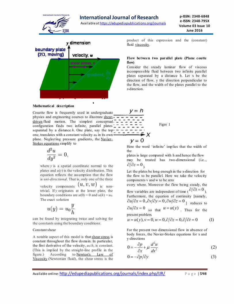
Mathematical description
Couette flow is frequently used in undergraduate
physics and engineering courses to illustrate shear-
driven fluid motion. The simplest conceptual
configuration finds two infinite, parallel plates
separated by a distance h. One plate, say the top
one, translates with a constant velocity u0 in its own
plane. Neglect ing pressure gradients, the Navier–
Stokes equations simplify to
where y is a spatial coordinate normal to the
plates and u(y) is the velocity d istribution. This
equation reflects the assumption that the flow
is uni-directional. That is, only one of the three
velocity components is non-
trivial. If y originates at the lower plate, the
boundary conditions are u(0) = 0 and u(h) = u0.
The exact solution
can be found by integrating twice and solving for
the constants using the boundary conditions.
Constant shear
A notable aspect of this model is that shear stress is
constant throughout the flow domain. In particular,
the first derivative of the velocity, u0/h, is constant.
(This is implied by the straight-line profile in the
figure.) According to Newton's Law of
Viscosity (Newtonian fluid), the shear stress is the
product of this expression and the (constant)
fluid viscosity.
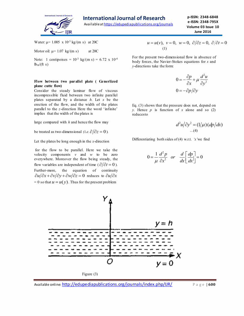
Flow between two parallel plate (Plane coutte
flow)
Consider the steady laminar flow of viscous
incompressible fluid between two infinite parallel
plates separated by a distance h. Let x be the
direction of flow, y the direction perpendicular to
the flow, and the width of the plates parallel to the
z-direction.
Figre 1
Here the word ‘infin ite’ implies that the width of
the
plates is large compared with h and hence the flow
may be treated has two-dimensional (i.e..,
0z ).
Let the plates be long enough in the x-direction for
the flow to be parallel. Here we take the velocity
components v and w to be zero
every where. Moreover the flow being steady, the
flow variables are independent of time (0t
).
Furthermore, the equation of continuity [namely,
0, 0, 0u x v y w z ] reduces to
0u x so that
( )u u y. Thus for the
present problem.
( ), 0, 0, 0, 0 (1)u u y v w z t
For the present two dimensional flow in absence of
body forces, the Navier-Stokes equations for x and
y-directions 2
20 (2)
0 (3)
p d u
x dx
p y
International Journal of Research Available at https://edupediapublications.org/journals
p-ISSN: 2348-6848 e-ISSN: 2348-795X
Volume 03 Issue 10 June 2016
Available online: http://edupediapublications.org/journals/index.php/IJR/ P a g e | 599
Equation (3) shows that the pressure does not
depend on y. Hence p is function of x alone and so
(2) reduces to 2
2
1(4)
d u dp
dy dx
Differentiating both sides of (4) with respect to ‘x’,
we find that 2
2
10 0
d p d dpor
dx dx dx
So that dp/dx = const = P (say) (5)
Then (4) reduces to 2
2
d u P
dy
(6)
Integrating (6),
du Py A
dx
(7)
Integrating (7),
2
2
Pu Ay B y
(8)
Where A and B are arbitrary constants to be
determined by the boundary conditions of the
problem under consideration.
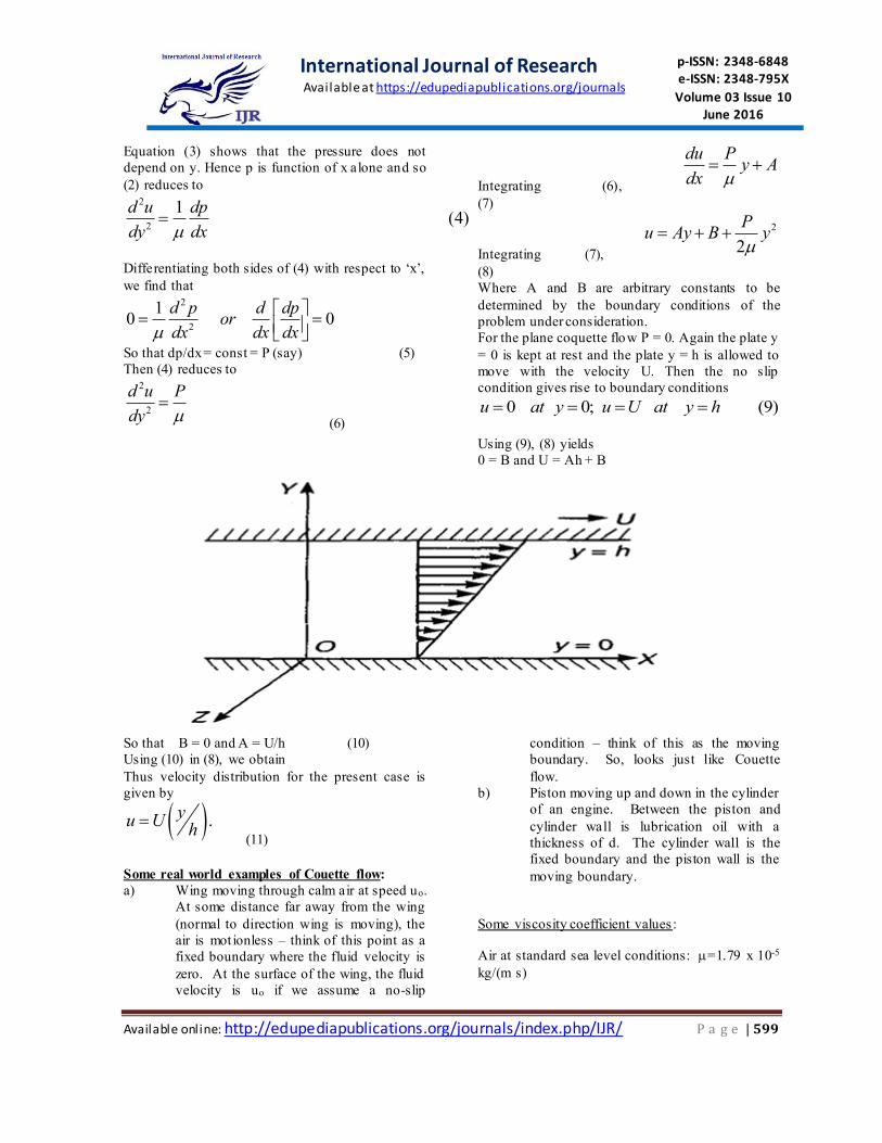
For the plane coquette flow P = 0. Again the plate y
= 0 is kept at rest and the plate y = h is allowed to
move with the velocity U. Then the no slip
condition gives rise to boundary conditions
0 0; (9)u at y u U at y h
Using (9), (8) yields
0 = B and U = Ah + B
Figure (2)
So that B = 0 and A = U/h (10)
Using (10) in (8), we obtain
Thus velocity distribution for the present case is
given by
.yu U
h
(11)
Some real world examples of Couette flow:
a) Wing moving through calm air at speed uo.
At some distance far away from the wing
(normal to direction wing is moving), the
air is mot ionless – think of this point as a
fixed boundary where the fluid velocity is
zero. At the surface of the wing, the fluid
velocity is uo if we assume a no-slip
condition – think of this as the moving
boundary. So, looks just like Couette
flow.
b) Piston moving up and down in the cylinder
of an engine. Between the piston and
cylinder wall is lubrication oil with a
thickness of d. The cylinder wall is the
fixed boundary and the piston wall is the
moving boundary.
Some viscosity coefficient values :
Air at standard sea level conditions: =1.79 x 10⁻⁵
kg/(m s)
International Journal of Research Available at https://edupediapublications.org/journals
p-ISSN: 2348-6848 e-ISSN: 2348-795X
Volume 03 Issue 10 June 2016
Available online: http://edupediapublications.org/journals/index.php/IJR/ P a g e | 600
Water: = 1.005 x 10⁻³ kg/(m s) at 20C
Motor oil: = 1.07 kg/(m s) at 20C
Note: 1 centipoises = 10-3 kg/(m s) = 6.72 x 10⁻⁴
lbm/(ft s)
Flow between two parallel plate ( Generlized
plane cutte flow)
Consider the steady laminar flow of viscous
incompressible fluid between two infinite parallel
plates separated by a distance h. Let x be the
erection of the flow, and the width of the plates
parallel to the z-direction Here the word ‘infinite’
implies that the width of the plates is
large compared with h and hence the flow may
be treated as two-dimensional (i.e. 0z ).
Let the plates be long enough in the x-direction
for the flow to be parallel. Here we take the
velocity components v and w to be zero
everywhere. Moreover the flow being steady, the
flow variables are independent of time ( 0t ).
Further-more, the equation of continuity
0u x v y w z reduces to u x
= 0 so that ( )u u y . Thus for the present problem
( ), 0, 0, 0, 0u u v v w z t
(1)
For the present two-dimensional flow in absence of
body forces, the Navier-Stokes equations for x and
y-directions take the form:
2
20 (2)
0 (3)
p d u
x y
p y
Eq. (3) shows that the pressure does not, depend on
y. Hence p is function of x alone and so (2)
reducesto
2 2 (1 )( )d u y dp dx …(4)
Differentiating both sides of (4) w.r.t. ‘x’we find
2
2
10 0
d p d dpor
x dx dx
Figure (3)
International Journal of Research Available at https://edupediapublications.org/journals
p-ISSN: 2348-6848 e-ISSN: 2348-795X
Volume 03 Issue 10 June 2016
Available online: http://edupediapublications.org/journals/index.php/IJR/ P a g e | 601
So that dp/dx=const. = P(say). …(5)
Then (4) reduces to 2 2d u dy P …(6)
Integrating (6), / P
du dy A
…(7)
Integrating (7), 2 / 2u Ay B Py …(8)
Where A and B are arbitrary constants to be determined by the boundary conditions of the flow problem under
consideration.
For the so called generalized plane Couette flow, the plate 0y are kept at rest and the plate y h is allowed
to move with velocity U. Then the no slip condition, gives rise to the following boundary conditions:
u = 0 at y = 0; u =U at y = h …(9)
Using these, (8) gives
O = B and U = Ah + B +
2
2
Ph
So that 0B and 2
U PhA
h
Using (9) in (8), we get
2
2 2
Uy Phy Pyu
h
Or
2
. 12
y h P y yu U
h h h
Or . 1u y y y
U h h h
Where
2
2
h P
U
Thus the velocity distribution for the present case is given by
International Journal of Research Available at https://edupediapublications.org/journals
p-ISSN: 2348-6848 e-ISSN: 2348-795X
Volume 03 Issue 10 June 2016
Available online: http://edupediapublications.org/journals/index.php/IJR/ P a g e | 602
. 1u y y y
U h h h
………(11)
Where
2
2
h P
U
To determine average and maximum velocities
The average velocity distribution for the present flow is given by
2 2
0
1 1( ,
hy
u dy U U y h y h dyh h h
Using (11)
= (1 2 6) ,U on simplification
Thus, (1 6) ( 3) . (13)u U
The volumetric flow Q per unit time per unit width of the channel is given by
(1 6) ( 3) .Q hu hu
From (11), 2
1 (14)du U U y
dy h h h
For the maximum or minimum velocity, 0du dy
That is 2
1 0U U y
h h h
giving
1 11 . (15)
2
y
h
From (15), it follows that the maximum velocity for 1 occurs at 1y h (that is )y h and the
minimum velocity for 1 at 0y h (that is 0).y This further shows that for 1 the velocity
gradient at the stationary wall is zero and it becomes negative for some value of 1. Thus the reverse
flow takes place when 1. Equation (15)breaks down when 1 1 because the maximum and
minimum values of y h have already been reached at 1 and 1 respectively. Using (15) in (14),
the maximum and minimum velocities are given by
2
max
2
min
(1 ) 4 , 1
{ (1 ) } 4 , 1
U U when
U U when
(16)
To determine shearing stress, skin friction and the coefficient of friction.
Using (14), the shearing stress distribution in the flow is given by
21 1yx
du U y
dy h h
(17)
International Journal of Research Available at https://edupediapublications.org/journals
p-ISSN: 2348-6848 e-ISSN: 2348-795X
Volume 03 Issue 10 June 2016
Available online: http://edupediapublications.org/journals/index.php/IJR/ P a g e | 603
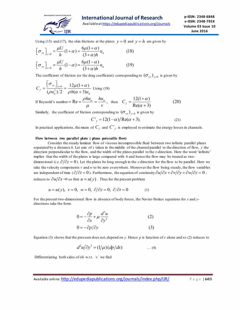
Using (13) and (17), the skin frictions at the plates 0y and y h are given by
0
6 (1 )(1 ) (18)
(3 )
6 (1 )(1 ) (19)
(3 )
yx y
yx y h
Uu
h h
Uu
h h
The coefficient of friction (or the drag coefficient) corresponding to 0( )yx y is given by
0
2
12 (1 )
( ) 2 ( 3)
yx y
fCu h u
Using (18)
If Reynold’s number Re ,hu hu
v
then
12(1 )(20)
Re( 3)fC
Similarly, the coefficient of friction corresponding to ( )yx y h is given by
' 12(1 ) Re( 3).fC (21)
In practical applications, the mean of fC and ' fC is employed to estimate the energy losses in channels.
Flow between two parallel plate ( plane poiseuille flow)
Consider the steady laminar flow of viscous incompressible fluid between two infinite parallel plates
separated by a distance h. Let axis of x taken in the middle of the channel parallel to the direction of flow, y the
direction perpendicular to the flow, and the width of the plates parallel to the z-direction. Here the word ‘infinite’
implies that the width of the plates is large compared with h and hence the flow may be treated as two-
dimensional (i.e. 0z ). Let the plates be long enough in the x-direction for the flow to be parallel. Here we
take the velocity components v and w to be zero everywhere. Moreover the flow being steady, the flow variables
are independent of time ( 0t ). Furthermore, the equation of continuity 0u x v y w z ;
reduces to u x =0 so that ( )u u y . Thus for the present problem
( ), 0, 0, 0, 0u u y v w z t (1)
For the present two-dimensional flow in absence of body forces, the Navier-Stokes equations for x and y-
directions take the form:
2
20 (2)
0 (3)
p d u
x y
p y
Equation (3) shows that the pressure does not, depend on y. Hence p is function of x alone and so (2) reduces to
2 2 (1 )( )d u y dp dx … (4)
Differentiating both sides of (4) w.r.t. ‘x’ we find
International Journal of Research Available at https://edupediapublications.org/journals
p-ISSN: 2348-6848 e-ISSN: 2348-795X
Volume 03 Issue 10 June 2016
Available online: http://edupediapublications.org/journals/index.php/IJR/ P a g e | 604
2
2
10 0
d p d dpor
x dx dx
So that dp/dx = const. = P (say). … (5)
Then (4) reduces to 2 2d u dy P … (6)
Integrating (6), / P
du dy A
… (7)
Integrating (7), 2 / 2u Ay B Py … (8)
Where A and B are arbitrary constants to be determined by the boundary conditions of the flow problem under
consideration.
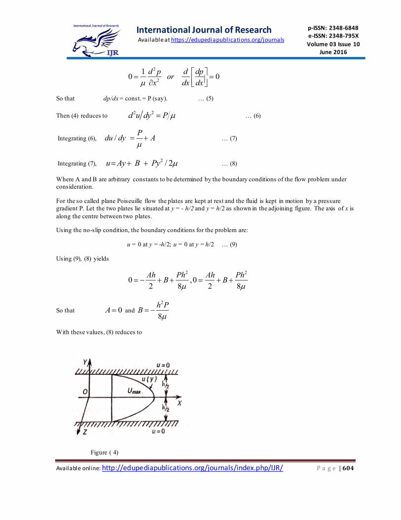
For the so called plane Poiseuille flow the plates are kept at rest and the fluid is kept in motion by a pressure
gradient P. Let the two plates lie situated at y = - h/2 and y = h/2 as shown in the adjoining figure. The axis of x is
along the centre between two plates.
Using the no-slip condition, the boundary conditions for the problem are:
u = 0 at y = -h/2; u = 0 at y = h/2 … (9)
Using (9), (8) yields
2 2
0 ,02 8 2 8
Ah Ph Ah PhB B
So that 0A and
2
8
h PB
With these values, (8) reduces to
Figure ( 4)
International Journal of Research Available at https://edupediapublications.org/journals
p-ISSN: 2348-6848 e-ISSN: 2348-795X
Volume 03 Issue 10 June 2016
Available online: http://edupediapublications.org/journals/index.php/IJR/ P a g e | 605
22
1 48
h P yu
h
… (10)
Showing that the velocity distribution for the flow is parabolic as shown in the figure 4
To determine the maximum and average velocities and shearing stress.
Eqn. (10) shows that the maximum velocity, umax, for the plane Poiseuille flow can be obtained by writing y = 0.
Thus
2
8maxu
h P
… (11)
Using (10), the average velocity distribution for the present flow is given by
22 2 3
2 2
max2 22 22
1 1 4 1 41
8 2 3
hh h
h hh
h p y y yu u dy dy u
h h h h h
, using (11)
Thus, ax(2 3) umu u on simplification … (12)
Combining (11) and (12), we have 212 ( )P u h … (13)
Using (10), the shearing stress distribution in the flow is given by
2
2
42
8yx
du h Py yP
dy h
… (14)
Then using (11), (12) and (14), the skin frictions at 2y h is given by
max
2
64 .
2yx y h
u uhP
h h
… (15)
Hence using (15), the frictional coefficient for laminar flow between two stationary plates is given by
2
2 2
6 2 1212
(1 2) Re
yx y h
f
uC
u h u hu
… (16)
Where Reynold’s number = Re = hu hu
v
BOUNDARY LAYER THEORY
International Journal of Research Available at https://edupediapublications.org/journals
p-ISSN: 2348-6848 e-ISSN: 2348-795X
Volume 03 Issue 10 June 2016
Available online: http://edupediapublications.org/journals/index.php/IJR/ P a g e | 606
The Navier-Stokes equations, it was observed that a
complete solution of these equations has not been
accomplished to date. This is particularly true when
friction and inertia forces are of the same order of
magnitude in the entire flow system, so that neither
can be neglected, we discussed some very special
cases of flow problems for which exact solutions of
the Navier-Stokes equations are possible. In those
cases, the equations were made linear by taking a
simple geometry of flow and assuming the flu id to
be incompressible. We dealt with a case of the
approximate solutions of the Navier-Stokes
equations for very small Reynold’s number. In that
chapter the frict ion forces far over-shadowed the
inertia forces, and the equations became linear by
omitting the convective acceleration. The present
chapter discusses the opposite, i.e., flow
characterized by very large Reynold’s numbers.
Prandtl’s boundary layer theory.
For convenience, consider laminar two-dimensional
flow of fluid of small viscosity (large Reynold’s
number) over a fixed semi-infinite plate. It is
observed that, unlike an ideal (non-viscous) fluid
flow, the fluid does not slide over the plate, but
“sticks” to it. Since the plate is at rest, the fluid in
contact with it will also be at rest. As we move
outwards along the normal, the velocity of the fluid
will gradually increase and at a d istance far from
the plate the full stream velocity U is attained.
Strict ly speaking this is approached asymptotically.
However, it will be assumed that the transition from
zero velocity at the p late to the full magnitude U
takes place within a thin layer of fluid in contact
with the plate. This is known as the boundary layer.
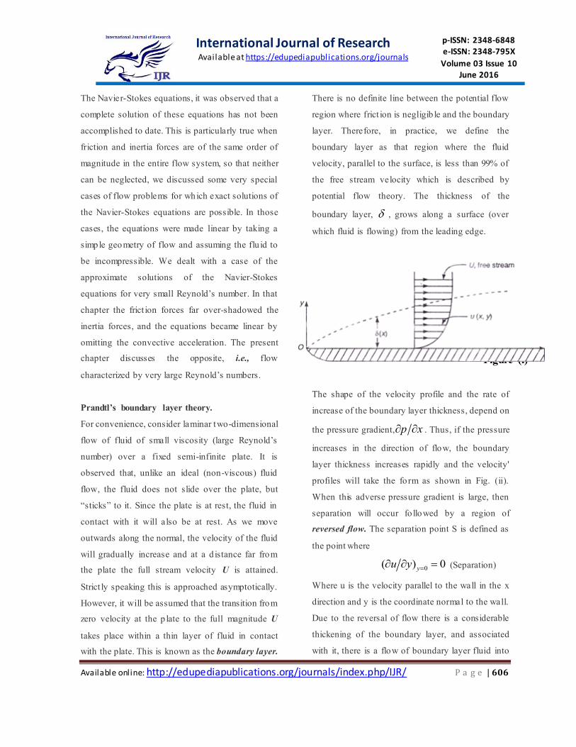
There is no definite line between the potential flow
region where frict ion is negligib le and the boundary
layer. Therefore, in practice, we define the
boundary layer as that region where the fluid
velocity, parallel to the surface, is less than 99% of
the free stream velocity which is described by
potential flow theory. The thickness of the
boundary layer, , grows along a surface (over
which fluid is flowing) from the leading edge.
The shape of the velocity profile and the rate of
increase of the boundary layer thickness, depend on
the pressure gradient, p x . Thus, if the pressure
increases in the direction of flow, the boundary
layer thickness increases rapidly and the velocity'
profiles will take the fo rm as shown in Fig. (ii).
When this adverse pressure gradient is large, then
separation will occur fo llowed by a region of
reversed flow. The separation point S is defined as
the point where
0( ) 0yu y (Separation)
Where u is the velocity parallel to the wall in the x
direction and y is the coordinate normal to the wall.
Due to the reversal of flow there is a considerable
thickening of the boundary layer, and associated
with it, there is a flow of boundary layer fluid into
Figure (i)
International Journal of Research Available at https://edupediapublications.org/journals
p-ISSN: 2348-6848 e-ISSN: 2348-795X
Volume 03 Issue 10 June 2016
Available online: http://edupediapublications.org/journals/index.php/IJR/ P a g e | 607
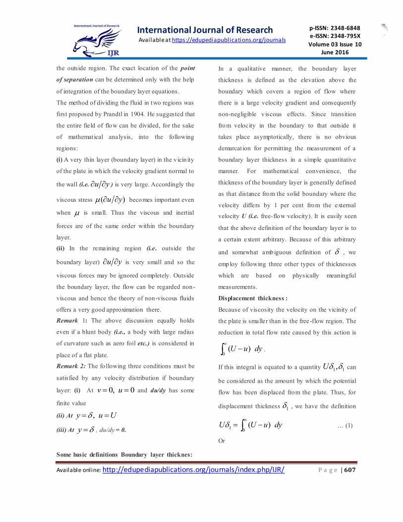
the outside region. The exact location of the point
of separation can be determined only with the help
of integration of the boundary layer equations.
The method of dividing the fluid in two regions was
first proposed by Prandtl in 1904. He suggested that
the entire field of flow can be divided, for the sake
of mathemat ical analysis, into the following
regions:
(i) A very thin layer (boundary layer) in the v icin ity
of the plate in which the velocity grad ient normal to
the wall (i.e. u y ) is very large. Accordingly the
viscous stress ( )u y becomes important even
when is small. Thus the viscous and inertial
forces are of the same order within the boundary
layer.
(ii) In the remaining region (i.e . outside the
boundary layer) u y is very small and so the
viscous forces may be ignored completely. Outside
the boundary layer, the flow can be regarded non-
viscous and hence the theory of non-viscous fluids
offers a very good approximation there.
Remark 1: The above discussion equally holds
even if a blunt body (i.e., a body with large radius
of curvature such as aero foil etc.) is considered in
place of a flat plate.
Remark 2: The fo llowing three conditions must be
satisfied by any velocity distribution if boundary
layer: (i) At 0, 0v u and du/dy has some
finite value
(ii) At ,y u U
(iii) At y , du/dy = 0.
Some basic definitions Boundary layer thicknes:
In a qualitative manner, the boundary layer
thickness is defined as the elevation above the
boundary which covers a region of flow where
there is a large velocity gradient and consequently
non-negligible v iscous effects. Since transition
from velocity in the boundary to that outside it
takes place asymptotically, there is no obvious
demarcat ion for permitting the measurement of a
boundary layer thickness in a simple quantitative
manner. For mathemat ical convenience, the
thickness of the boundary layer is generally defined
as that distance from the solid boundary where the
velocity differs by 1 per cent from the external
velocity U (i.e. free-flow velocity). It is easily seen
that the above definition of the boundary layer is to
a certain extent arbitrary. Because of this arbitrary
and somewhat ambiguous definition of , we
employ following three other types of thicknesses
which are based on physically meaningful
measurements.
Displacement thickness :
Because of viscosity the velocity on the vicinity of
the plate is smaller than in the free -flow region. The
reduction in total flow rate caused by this action is
0( )U u dy
.
If this integral is equated to a quantity 1 1,U can
be considered as the amount by which the potential
flow has been displaced from the p late. Thus, for
displacement thickness 1 , we have the definition
10
( )U U u dy
… (1)
Or
International Journal of Research Available at https://edupediapublications.org/journals
p-ISSN: 2348-6848 e-ISSN: 2348-795X
Volume 03 Issue 10 June 2016
Available online: http://edupediapublications.org/journals/index.php/IJR/ P a g e | 608
10
(1 / )u U dy
…
(2)
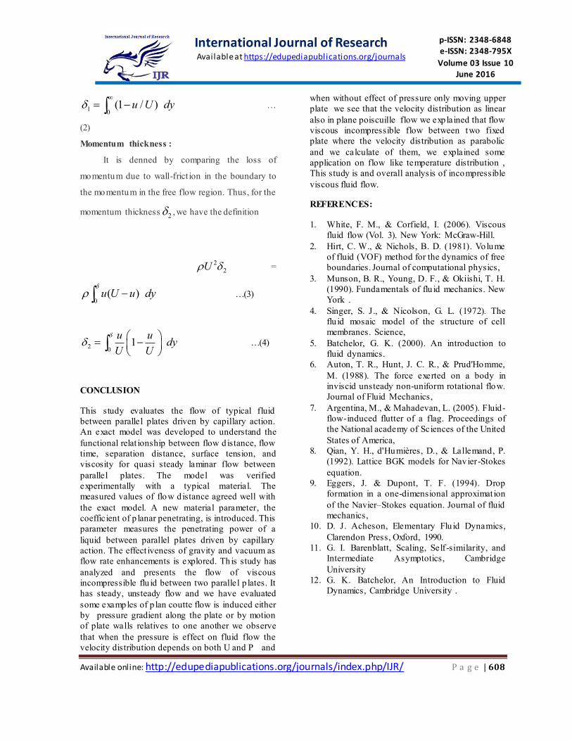
Momentum thickness :
It is denned by comparing the loss of
momentum due to wall-frict ion in the boundary to
the momentum in the free flow region. Thus, for the
momentum thickness 2 , we have the definition
2
2U =
0( )u U u dy
…(3)
20
1u u
dyU U
…(4)
CONCLUSION
This study evaluates the flow of typical fluid
between parallel plates driven by capillary action.
An exact model was developed to understand the
functional relat ionship between flow d istance, flow
time, separation distance, surface tension, and
viscosity for quasi steady laminar flow between
parallel plates. The model was verified
experimentally with a typical material. The
measured values of flow d istance agreed well with
the exact model. A new material parameter, the
coefficient of p lanar penetrating, is introduced. This
parameter measures the penetrating power of a
liquid between parallel plates driven by capillary
action. The effect iveness of gravity and vacuum as
flow rate enhancements is explored. Th is study has
analyzed and presents the flow of viscous
incompressible flu id between two parallel p lates. It
has steady, unsteady flow and we have evaluated
some examples of p lan coutte flow is induced either
by pressure gradient along the plate or by motion
of plate walls relatives to one another we observe
that when the pressure is effect on fluid flow the
velocity distribution depends on both U and P and
when without effect of pressure only moving upper
plate we see that the velocity distribution as linear
also in plane poiscuille flow we exp lained that flow
viscous incompressible flow between two fixed
plate where the velocity distribution as parabolic
and we calculate of them, we explained some
application on flow like temperature distribution ,
This study is and overall analysis of incompressible
viscous fluid flow.
REFERENCES:
1. White, F. M., & Corfield, I. (2006). Viscous
fluid flow (Vol. 3). New York: McGraw-Hill.
2. Hirt, C. W., & Nichols, B. D. (1981). Volume
of fluid (VOF) method for the dynamics of free
boundaries. Journal of computational physics,
3. Munson, B. R., Young, D. F., & Okiishi, T. H.
(1990). Fundamentals of flu id mechanics. New
York .
4. Singer, S. J., & Nicolson, G. L. (1972). The
flu id mosaic model of the structure of cell
membranes. Science,
5. Batchelor, G. K. (2000). An introduction to
fluid dynamics.
6. Auton, T. R., Hunt, J. C. R., & Prud'Homme,
M. (1988). The force exerted on a body in
inviscid unsteady non-uniform rotational flow.
Journal of Fluid Mechanics,
7. Argentina, M., & Mahadevan, L. (2005). Fluid-
flow-induced flutter of a flag. Proceedings of
the National academy of Sciences of the United
States of America,
8. Qian, Y. H., d'Humières, D., & Lallemand, P.
(1992). Lattice BGK models for Navier-Stokes
equation.
9. Eggers, J. & Dupont, T. F. (1994). Drop
formation in a one-dimensional approximat ion
of the Navier–Stokes equation. Journal of fluid
mechanics,
10. D. J. Acheson, Elementary Flu id Dynamics,
Clarendon Press, Oxford, 1990.
11. G. I. Barenblatt, Scaling, Self-similarity, and
Intermediate Asymptotics, Cambridge
University
12. G. K. Batchelor, An Introduction to Fluid
Dynamics, Cambridge University .

![Incompressible Viscous Fluid Flows in a Thin Spherical Shell · Vol. 11 (2009) Incompressible Viscous Fluid Flows in a Thin Spherical Shell 61 More recent work of Furnier et al. [13]](https://img.pdfslide.net/doc/110x75/5f6a892643dbc81aca4490dc/incompressible-viscous-fluid-flows-in-a-thin-spherical-shell-vol-11-2009-incompressible.jpg)


![Small moving rigid body into a viscous incompressible fluid · Iftimie, Lopes Filho and Nussenzveig Lopes [21] have studied the case of one small fixed obstacle in an incompressible](https://img.pdfslide.net/doc/110x75/5c2e7a9d09d3f2f90b8c7b0c/small-moving-rigid-body-into-a-viscous-incompressible-fluid-iftimie-lopes-filho.jpg)