A Supply and Demand Based Volatility Model

for Energy Prices- The Relationship between Supply Curve Shape and Volatility -∗

Takashi Kanamura†‡

First draft: February 8, 2006

This draft: September 17, 2006

ABSTRACT

This paper proposes a new volatility model for energy prices explicitly characterizedby the supply-demand relationship, which we call a Supply and Demand based Volatility(SDV) model. We show that the supply curve shape of energy in the SDV model producesthe characteristics of the volatility in energy prices. Especially, it is found that the inverseBox-Cox transformation supply curve reflecting energy markets appropriately causes theinverse leverage effect often seen in the markets. The SDV model is also used to showthat an existing (G)ARCH-M model has foundation on the supply-demand relationship.In addition, we conduct the empirical studies analyzing the volatility in the U.S. naturalgas prices.

Key words: Energy prices, volatility, supply curve, inverse Box-Cox transformation,inverse leverage effect, volatility-in-mean effect, natural gasJEL Classification: C51, L97, Q40

∗Views expressed in this paper are those of the author and do not necessarily reflect those of J-POWER.I am grateful to Toshiki Honda, Shoji Kamimura, Matteo Manera, Ryozo Miura, Izumi Nagayama, NobuhiroNakamura, Makoto Nakano, Mikiharu Noma, and especially KazuhikoOhashi for their useful comments andsuggestions. I also wish to thank Juri Hinz, Christoph Reisinger, Ryosuke Wada, and all seminar participantsat the Bachelier Finance Society 2006 Fourth World Congress for their helpful comments and suggestions. Allremaining errors are mine.

†J-POWER, Japan‡Address correspondence to Takashi Kanamura, J-POWER, 15-1, Ginza 6-Chome, Chuo-ku, Tokyo 104-

8165. Phone: +81-3-3546-9623. Fax: +81-3-3546-9531. E-mail: tkanamura@ics.hit-u.ac.jp

1. Introduction

This paper proposes a volatility model for energy prices explicitly characterized by the supply-

demand relationship, which we call a Supply and Demand based Volatility (SDV) model. In

addition, it empirically analyzes the U.S. natural gas market by using the model.

High volatility in price returns often appears in deregulated energy markets. The volatility

affects the market participants, such as energy producers and distributors. As a simple example

to illustrate the influence of the volatility, let us think of a thermal power plant procuring

the fuel, such as natural gas, from the spot market. Since the prices are volatile due to the

supply and demand in the market, the risk manager in charge of the plant needs to capture the

volatility as accurately as possible by using an energy volatility model. As described in the

above example, the volatility models have been introduced into energy markets.

Although a lot of volatility models both in continuous and discrete time were developed in

financial markets, they are directly applied to the volatility models in energy markets without

any adjustment for the energy characteristics. The continuous time models in stock markets,

such as Heston model introduced by Heston (1993) and C.E.V. (Constant Elasticity of Vari-

ance) models developed by Cox (1975) and extended by Emanuel and MacBeth (1982), are

directly used for the models in energy markets (e.g., Eydeland and Wolyniec (2003)). Sim-

ilarly, the discrete time models such as ARCH, GARCH, and ARCH-M models in Engle

(1982), Bollerslev (1986), and Engle, Lilien, and Robins (1987) are employed in the energy

market models in Duffie, Gray, and Hoang (1999), Pindyck (2004), and Deaves and Krinsky

(1992), respectively.

Energy markets may utilize the same volatility models as financial markets. However,

the volatility in energy markets is not necessarily the same as that in stock markets. For

instance, energy markets exhibit stronger seasonality in the volatility than financial markets.

In addition, the “inverse leverage effect”, i.e., volatility increases in prices, often appears

in energy markets, while the analyses in stock markets illustrate the opposite relationship

1

� ����� ����� ����� ���� � ���� �����

� �� ��

�

�

�

�

�

�

�

��������� �� ���

"!�#%$�&�')(+*)*),.-0/

132�4.576�8+29,:$�;< =$�50$

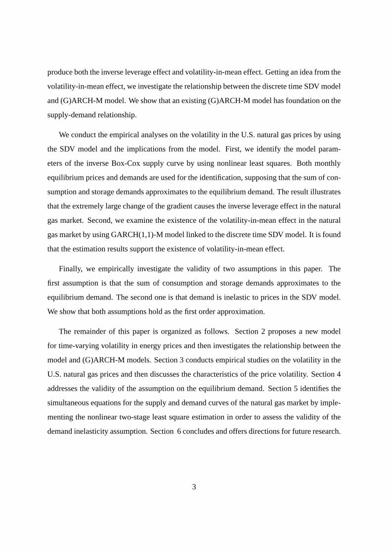
Figure 1. The Relationship between Demand (=Supply) and Prices

between the volatility and the prices.1 This paper proposes the SDV model for energy prices

that can accurately express the characteristics of volatility in energy prices by using the supply-

demand relationship.

Observing the scatter diagram with the axes of equilibrium prices and demands for natural

gas in the U.S. as in Figure 1, the plots seem scattered along with an upward-sloping curve. In

order to express the curve by using a simple model, we introduce an equilibrium price model

determined by the inelastic demand curve fluctuating stochastically and the upward-sloping

supply curve fixed in a short period of time. We show that the price model provides twofold

characteristics of the volatility in energy price returns. First, the volatility is time varying

owing to both the upward-sloping supply curve and demand shocks. Second, the mean of

price returns changes with the volatility, which we call “volatility-in-mean effect”, due to the

drift term of price returns represented by the function of the volatility. Then, we specify the

model by employing the inverse Box-Cox transformation supply curve that can exhibit the

drastic slope changes with an appropriate function parameter. It is found that the model can

1The opposite is called “leverage effect” such that volatility falls as prices rise.

2

produce both the inverse leverage effect and volatility-in-mean effect. Getting an idea from the

volatility-in-mean effect, we investigate the relationship between the discrete time SDV model

and (G)ARCH-M model. We show that an existing (G)ARCH-M model has foundation on the

supply-demand relationship.

We conduct the empirical analyses on the volatility in the U.S. natural gas prices by using

the SDV model and the implications from the model. First, we identify the model param-

eters of the inverse Box-Cox supply curve by using nonlinear least squares. Both monthly

equilibrium prices and demands are used for the identification, supposing that the sum of con-

sumption and storage demands approximates to the equilibrium demand. The result illustrates

that the extremely large change of the gradient causes the inverse leverage effect in the natural

gas market. Second, we examine the existence of the volatility-in-mean effect in the natural

gas market by using GARCH(1,1)-M model linked to the discrete time SDV model. It is found

that the estimation results support the existence of volatility-in-mean effect.

Finally, we empirically investigate the validity of two assumptions in this paper. The

first assumption is that the sum of consumption and storage demands approximates to the

equilibrium demand. The second one is that demand is inelastic to prices in the SDV model.

We show that both assumptions hold as the first order approximation.

The remainder of this paper is organized as follows. Section 2 proposes a new model

for time-varying volatility in energy prices and then investigates the relationship between the

model and (G)ARCH-M models. Section 3 conducts empirical studies on the volatility in the

U.S. natural gas prices and then discusses the characteristics of the price volatility. Section 4

addresses the validity of the assumption on the equilibrium demand. Section 5 identifies the

simultaneous equations for the supply and demand curves of the natural gas market by imple-

menting the nonlinear two-stage least square estimation in order to assess the validity of the

demand inelasticity assumption. Section 6 concludes and offers directions for future research.

3

2. The Model

2.1. A Supply and Demand based Volatility (SDV) model for energy prices

Figure 1 illustrates the relationship between monthly equilibrium demands and prices for nat-

ural gas in the U.S..2 As we see, the plots seem scattered around a single monotone increasing

convex curve. The market observation has motivated us to model energy spot prices and the

volatility by incorporating the relationship directly.

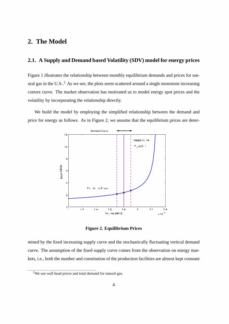
We build the model by employing the simplified relationship between the demand and

price for energy as follows. As in Figure 2, we assume that the equilibrium prices are deter-

� ����� ����� ����� ���� � ���� ������ �� ��

�

�

�

��

���

��������� �� ���

���� �!�"$#$%'&$&$(*),+

- !�.�.� �/102!�3546#

798;:=<�% - 8;+

>?#�"A@�B�C$0D!�3546#

EGF�!�H� IHIJ�3'HI!�"K7G3'HI(L#�M

Figure 2. Equilibrium Prices

mined by the fixed increasing supply curve and the stochastically fluctuating vertical demand

curve. The assumption of the fixed supply curve comes from the observation on energy mar-

kets, i.e., both the number and constitution of the production facilities are almost kept constant

2We use well head prices and total demand for natural gas.

4

in a short term. The assumption of the vertical demand curve arises from the demand inelas-

ticity to prices in the short run, i.e., energy use seems to be independent of the price change in

that period.3 In this sense, the model is considered as the first order approximation. The idea

has been already applied to the spot price model for electricity as in Barlow (2002) and Kana-

mura andOhashi (2006). It should be noted that as in Figure 2 the model is able to generate

the large rate of price change with respect to the demand as the demand (i.e., price) increases,

supposing that the supply curve is dramatically upward sloping.

Based on the above idea, we formulate the model as follows. We denote the fixed sup-

ply curve for energy byPt = g(St) which is the second order differentiable, monotone, and

increasing convex function with respect to the supplySt . On the assumption of the demand

inelasticity, the equilibrium prices are determined by the supply curve function replacing the

supplySt by the demandDt :

Pt = g(Dt). (1)

Next, we model the demand for energy, assuming that it consists ofn components4:

Dt =n

∑i=1

Dit (2)

and that each of the demands follows a stochastic process:

dDit =µi

Ddt+σiDdwi

t (3)

whereEt [dwitdwj

t ] = ρi j dt.

3People continue to consume energy even though the price increases more or less, because it is mainly usedfor adjustment of room temperature by heating and cooling. Especially, this assumption holds well for electricityprices.

4Consumption and storage demands are the examples.

5

Proposition 1 Suppose that equilibrium prices for energy are given by the function of the

demand asPt = g(Dt) where the demand process is generated by Eqs. (2) and (3). Then, a

Supply and Demand based Volatility (SDV) model for energy prices is expressed as follows:

dPt

Pt=µtdt+σtdwt (4)

σt =g′(Dt)g(Dt)

σD (5)

µt =(

µD

σD+

12

g′′(Dt)g′(Dt)

σD

)σt (6)

µD =n

∑i=1

µiD, σD =

√n

∑i, j=1

σiDσ j

Dρi j , dwt =1

σD

n

∑i=1

σiDdwi

t .

Proof We apply Ito’s Lemma to Eq. (1) by using Eqs. (2) and (3).‖

Eq. (5) shows that the volatilityσt is proportional to the ratio of the first derivative to

the level of the supply curve functiong, which causes time-varying volatility by the demand

shocks as long asg′(Dt)

g(Dt)is not reducible. Moreover, the drift term in Eq. (6) changes with the

volatility, which leads to the existence of the volatility-in-mean effect. In addition, since the

supply curveg is the second order differentiable, monotonic, and increasing convex function,g′′(D)g(D) ≥ 0 holds in Eq. (6). It implies that the volatility positively affects the drift term in

Eq.(6), whenµD is greater than or equal to 0. As we have mentioned, the simplest model

for energy prices based on the supply-demand relationship even can produce two significant

characteristics on the volatility. First, the model exhibits time-varying property, since the

volatility of the price returns depends on the demand. Second, there exists the volatility-in-

mean effect since the drift term of price returns is the function of the volatility. In an effort to

deepen the discussion on the volatility, the next section explicitly specifies the supply curve

function that reflects energy markets more appropriately.

6

2.2. One-factor SDV model for energy prices

In order to examine the characteristics of the SDV model in detail, we propose one-factor SDV

model for energy prices that is tractable and whose solution exists by employing an explicit

supply function that reflects an energy market observation. The exponential function may

be a reasonable choice to express the second order differentiable, monotonic, and increasing

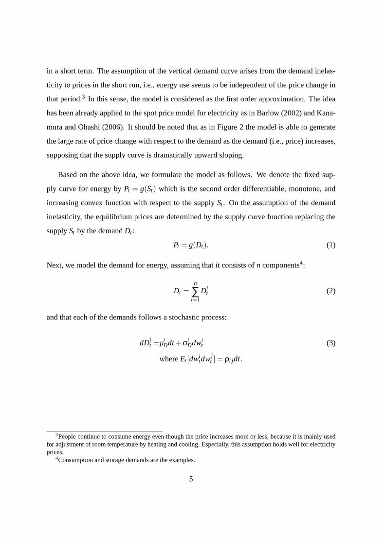
convex function assumed in Proposition 1. However, Figure 3 regressing the exponential curve

on the data as in Figure 15 implies that the rate of change of price with respect to the demand

� ����� � �����

� ���

�

�

�

�

�

�

�

��������� �� ���

��� �"! # $"%'&"&"(*),+

-/.�0*132�4'.5(6! 76$�!1,!8 �:9 2�# � #1,.5!�7606; 9 9 7�<=(6;�4?>:�

Figure 3. Supply Curves

for the scatter plots seems to be much larger than that for the exponential function. For this

reason, we employ the inverse Box-Cox transformation as the supply curve that can not only

have the exponential function built in but also exhibit larger gradients of the supply curve

than the exponential function, although there exists a problem on the asymptote for the supply

5The parameters are obtained by the nonlinear least square method as in Appendix E.

7

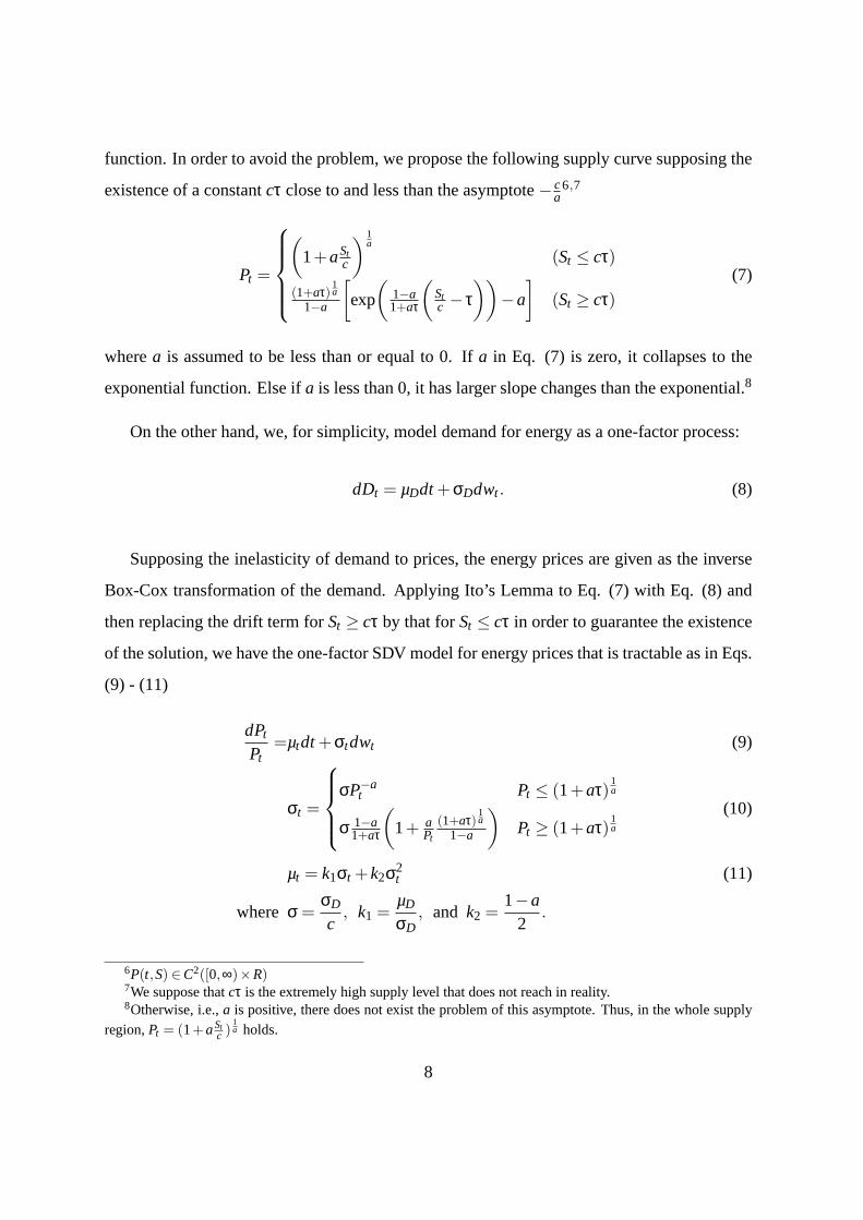
function. In order to avoid the problem, we propose the following supply curve supposing the

existence of a constantcτ close to and less than the asymptote− ca

6,7

Pt =

(1+aSt

c

) 1a

(St ≤ cτ)

(1+aτ)1a

1−a

[exp

(1−a1+aτ

(Stc − τ

))−a

](St ≥ cτ)

(7)

wherea is assumed to be less than or equal to 0. Ifa in Eq. (7) is zero, it collapses to the

exponential function. Else ifa is less than 0, it has larger slope changes than the exponential.8

On the other hand, we, for simplicity, model demand for energy as a one-factor process:

dDt = µDdt+σDdwt . (8)

Supposing the inelasticity of demand to prices, the energy prices are given as the inverse

Box-Cox transformation of the demand. Applying Ito’s Lemma to Eq. (7) with Eq. (8) and

then replacing the drift term forSt ≥ cτ by that forSt ≤ cτ in order to guarantee the existence

of the solution, we have the one-factor SDV model for energy prices that is tractable as in Eqs.

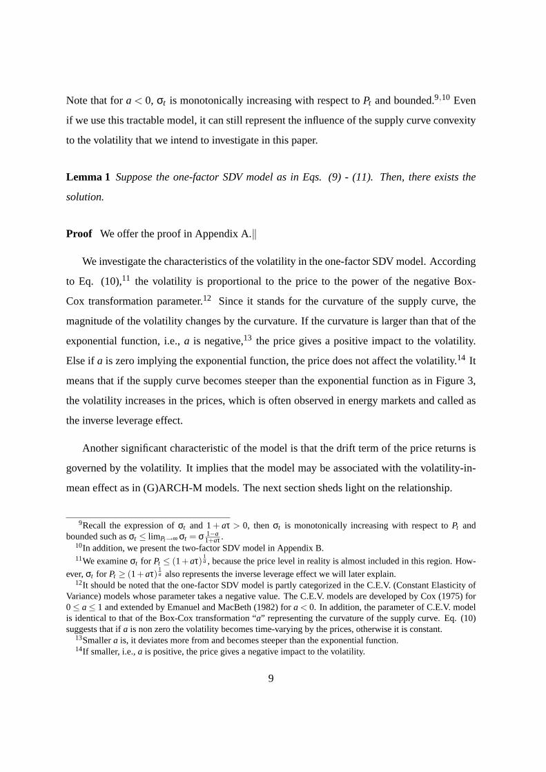
(9) - (11)

dPt

Pt=µtdt+σtdwt (9)

σt =

σP−at Pt ≤ (1+aτ)

1a

σ 1−a1+aτ

(1+ a

Pt

(1+aτ)1a

1−a

)Pt ≥ (1+aτ)

1a

(10)

µt = k1σt +k2σ2t (11)

where σ =σD

c, k1 =

µD

σD, and k2 =

1−a2

.

6P(t,S) ∈C2([0,∞)×R)7We suppose thatcτ is the extremely high supply level that does not reach in reality.8Otherwise, i.e.,a is positive, there does not exist the problem of this asymptote. Thus, in the whole supply

region,Pt = (1+aStc )

1a holds.

8

Note that fora < 0, σt is monotonically increasing with respect toPt and bounded.9,10 Even

if we use this tractable model, it can still represent the influence of the supply curve convexity

to the volatility that we intend to investigate in this paper.

Lemma 1 Suppose the one-factor SDV model as in Eqs. (9) - (11). Then, there exists the

solution.

Proof We offer the proof in Appendix A.‖

We investigate the characteristics of the volatility in the one-factor SDV model. According

to Eq. (10),11 the volatility is proportional to the price to the power of the negative Box-

Cox transformation parameter.12 Since it stands for the curvature of the supply curve, the

magnitude of the volatility changes by the curvature. If the curvature is larger than that of the

exponential function, i.e.,a is negative,13 the price gives a positive impact to the volatility.

Else if a is zero implying the exponential function, the price does not affect the volatility.14 It

means that if the supply curve becomes steeper than the exponential function as in Figure 3,

the volatility increases in the prices, which is often observed in energy markets and called as

the inverse leverage effect.

Another significant characteristic of the model is that the drift term of the price returns is

governed by the volatility. It implies that the model may be associated with the volatility-in-

mean effect as in (G)ARCH-M models. The next section sheds light on the relationship.

9Recall the expression ofσt and 1+ aτ > 0, then σt is monotonically increasing with respect toPt andbounded such asσt ≤ limPt→∞ σt = σ 1−a

1+aτ .10In addition, we present the two-factor SDV model in Appendix B.11We examineσt for Pt ≤ (1+aτ)

1a , because the price level in reality is almost included in this region. How-

ever,σt for Pt ≥ (1+aτ)1a also represents the inverse leverage effect we will later explain.

12It should be noted that the one-factor SDV model is partly categorized in the C.E.V. (Constant Elasticity ofVariance) models whose parameter takes a negative value. The C.E.V. models are developed by Cox (1975) for0≤ a≤ 1 and extended by Emanuel and MacBeth (1982) fora < 0. In addition, the parameter of C.E.V. modelis identical to that of the Box-Cox transformation “a” representing the curvature of the supply curve. Eq. (10)suggests that ifa is non zero the volatility becomes time-varying by the prices, otherwise it is constant.

13Smallera is, it deviates more from and becomes steeper than the exponential function.14If smaller, i.e.,a is positive, the price gives a negative impact to the volatility.

9

2.3. Why is (G)ARCH-M model applied to energy prices?

Many previous works on energy markets introduce (G)ARCH models to capture the het-

eroskedasticity of the volatility in the prices. However, to our knowledge the goodness of

fit to market data seems the main reason for the model selection. This section, then, offers an

economic reason behind the selection of a (G)ARCH-M model for energy prices employing

the SDV model.

To investigate the relationship between the SDV model to (G)ARCH models, we represent

the SDV model in discrete time transformed from that in continuous one as in Eqs. (9) and

(11) as follows:

rt = µt +σtεt , µt = µ1σt +µ2σ2t (12)

wherert = log(Pt+1)− log(Pt), µ1 = µD(Dt)σD

, and µ2 = −a2. Using Eqs. (7) and (10),15 σ2

t

leads to the function of demand for energy:

σ2t =

σ2D

(c+aDt)2 . (13)

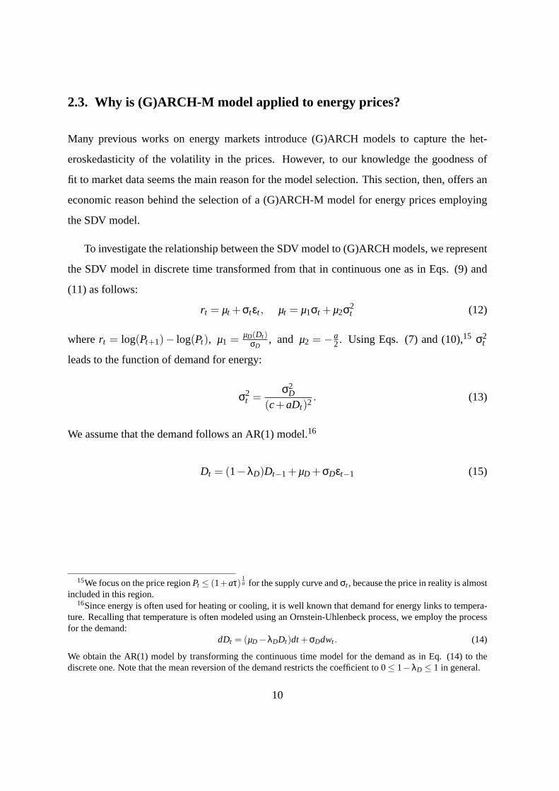
We assume that the demand follows an AR(1) model.16

Dt = (1−λD)Dt−1 +µD +σDεt−1 (15)

15We focus on the price regionPt ≤ (1+aτ)1a for the supply curve andσt , because the price in reality is almost

included in this region.16Since energy is often used for heating or cooling, it is well known that demand for energy links to tempera-

ture. Recalling that temperature is often modeled using an Ornstein-Uhlenbeck process, we employ the processfor the demand:

dDt = (µD−λDDt)dt+σDdwt . (14)

We obtain the AR(1) model by transforming the continuous time model for the demand as in Eq. (14) to thediscrete one. Note that the mean reversion of the demand restricts the coefficient to0≤ 1−λD ≤ 1 in general.

10

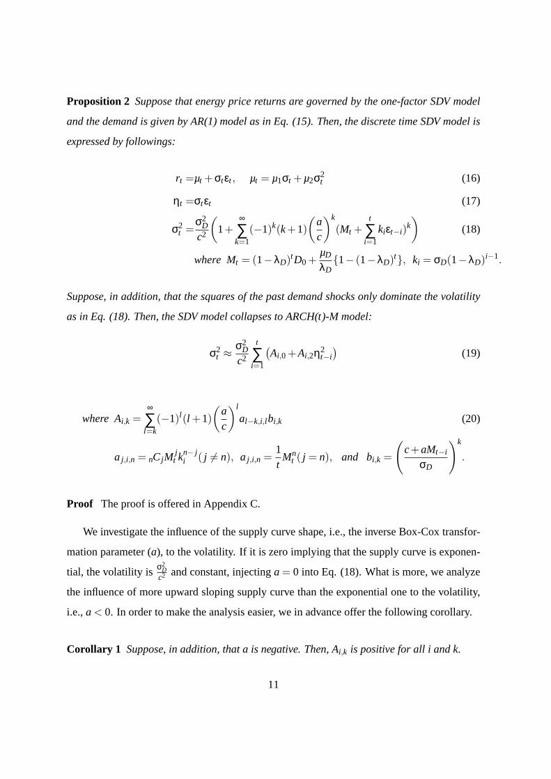
Proposition 2 Suppose that energy price returns are governed by the one-factor SDV model

and the demand is given by AR(1) model as in Eq. (15). Then, the discrete time SDV model is

expressed by followings:

rt =µt +σtεt , µt = µ1σt +µ2σ2t (16)

ηt =σtεt (17)

σ2t =

σ2D

c2

(1+

∞

∑k=1

(−1)k(k+1)(

ac

)k

(Mt +t

∑i=1

kiεt−i)k)

(18)

where Mt = (1−λD)tD0 +µD

λD{1− (1−λD)t}, ki = σD(1−λD)i−1.

Suppose, in addition, that the squares of the past demand shocks only dominate the volatility

as in Eq. (18). Then, the SDV model collapses to ARCH(t)-M model:

σ2t ≈

σ2D

c2

t

∑i=1

(Ai,0 +Ai,2η2

t−i

)(19)

where Ai,k =∞

∑l=k

(−1)l (l +1)(

ac

)l

al−k,i,l bi,k (20)

a j,i,n = nCjMjt kn− j

i ( j 6= n), a j,i,n =1tMn

t ( j = n), and bi,k =

(c+aMt−i

σD

)k

.

Proof The proof is offered in Appendix C.

We investigate the influence of the supply curve shape, i.e., the inverse Box-Cox transfor-

mation parameter (a), to the volatility. If it is zero implying that the supply curve is exponen-

tial, the volatility is σ2D

c2 and constant, injectinga = 0 into Eq. (18). What is more, we analyze

the influence of more upward sloping supply curve than the exponential one to the volatility,

i.e.,a < 0. In order to make the analysis easier, we in advance offer the following corollary.

Corollary 1 Suppose, in addition, thata is negative. Then,Ai,k is positive for alli andk.

11

Proof The proof is given in Appendix D.

The corollary suggests that ifa is negative, then the volatility in Eq. (19) always increases

in the past demand shocks, because it includes the squares of the past demand shocks and the

positive coefficients. In addition, the negativea guarantees nonnegativeness ofσ2t in Eq. (19).

It is well-known that AR(∞) collapses to GARCH(1,1), taking timet as infinity. The

volatility, then, is likely to be modeled by ARCH(t) or GARCH(1,1) models, if the squares of

the past demand shocks approximately dominate it. Recalling that as in Eq. (16), the model

accommodates the volatility-in-mean effect, an existing GARCH(1,1)-M model for energy

prices has foundation on the supply-demand relationship.

Using the simple supply curve that reflects energy markets, Section 2 obtained the SDV

model that can produce both the inverse leverage and volatility-in-mean effects. Justifying the

model for energy prices, Section 3 is devoted to empirically analyze the volatility in the U.S.

natural gas prices.

3. Empirical Studies on the U.S. Natural Gas Price Volatility

3.1. Data

We use historical prices, storage, and consumption for the U.S. natural gas to analyze the char-

acteristics of the price volatility. The wellhead prices are used as the proxy of the equilibrium

prices owing to data availability. The storage and consumption are employed to calculate the

total equilibrium demand. These data are originally provided by the Energy Information Ad-

ministration (EIA),17 including 339 monthly observations from January 1976 to March 2004,

respectively.

17As of the first two data, we directly download them from the homepage of the EIA. The data is obtainedfrom www.eia.doe.gov. On the other hand, the website of Economagic.com offers the consumption demandscollected from the EIA.

12

3.2. Inverse leverage effect in the U.S. natural gas market

As we modeled in Section 2.2, the volatility of the one-factor SDV model is the function of the

price whose parameter represents the curvature of the supply curve shape. Using the volatility

model whose parameter is estimated from the U.S. natural gas market, we, then, show that the

supply curve shape causes the inverse leverage effect: the increase of volatility in prices.

Supposing that demand for natural gas is approximately inelastic to the prices, the demand-

price relationship leads to the supply curve. Thus, the equilibrium prices are a monotonically

increasing function of the equilibrium demands. To estimate the supply curve (demand-price

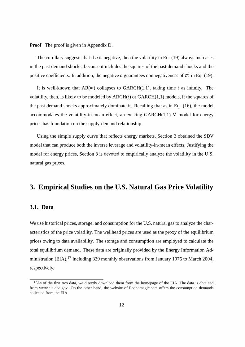
relationship), we need to identify the equilibrium demands. Figure 4 illustrates the scatter

� ��� ��� � �� �����

�

�

�

�

�

�������������������������� �!�!�"$#&%

')(*)+,-. /0+12

Figure 4. Storage Demands / Prices

����� � ����� � ����� � ����

�

�

�

�

�

�

�

��������������������� �"!#��$���%�&('�'�)+*-,

.0/102345 67289

Figure 5. Consumption Demands / Prices

plots between storage demands18 in x-axis and the prices iny-axis for the natural gas from

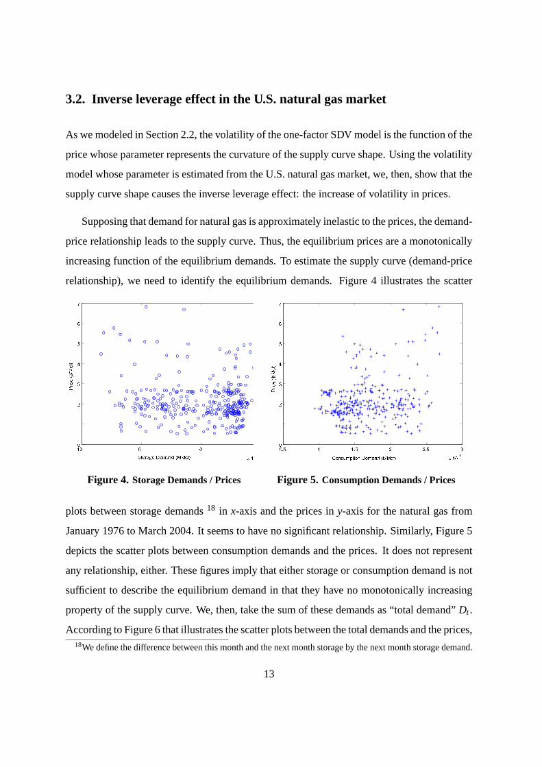
January 1976 to March 2004. It seems to have no significant relationship. Similarly, Figure 5

depicts the scatter plots between consumption demands and the prices. It does not represent

any relationship, either. These figures imply that either storage or consumption demand is not

sufficient to describe the equilibrium demand in that they have no monotonically increasing

property of the supply curve. We, then, take the sum of these demands as “total demand”Dt .

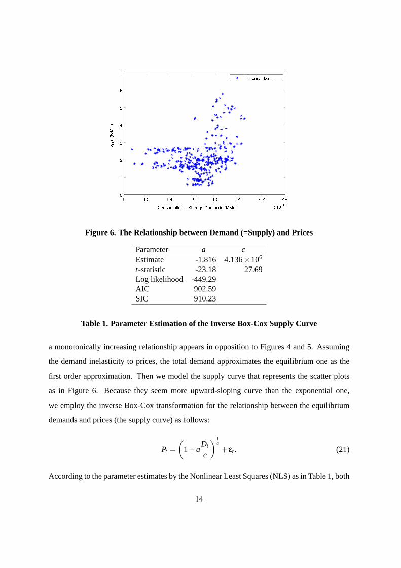
According to Figure 6 that illustrates the scatter plots between the total demands and the prices,18We define the difference between this month and the next month storage by the next month storage demand.

13

� ����� ����� ����� ���� � ���� �����

� �� ��

�

�

�

�

�

�

�

��������� �� ���

"!�#�$&%�')(�*,+-!�#).0/1*,!�243�5�68796�')3�#�:�$<;4=)=)>@?BA

C +�$@*B!�24+->&3�DE7F3�*,3

Figure 6. The Relationship between Demand (=Supply) and Prices

Parameter a cEstimate -1.816 4.136×106

t-statistic -23.18 27.69Log likelihood -449.29AIC 902.59SIC 910.23

Table 1. Parameter Estimation of the Inverse Box-Cox Supply Curve

a monotonically increasing relationship appears in opposition to Figures 4 and 5. Assuming

the demand inelasticity to prices, the total demand approximates the equilibrium one as the

first order approximation. Then we model the supply curve that represents the scatter plots

as in Figure 6. Because they seem more upward-sloping curve than the exponential one,

we employ the inverse Box-Cox transformation for the relationship between the equilibrium

demands and prices (the supply curve) as follows:

Pt =(

1+aDt

c

) 1a

+ εt . (21)

According to the parameter estimates by the Nonlinear Least Squares (NLS) as in Table 1, both

14

� ����� � �����

� ���

�

�

�

�

��

��

��������� �� ���

�����! �"�#!$&%!%!')(+*

,.-0/)1+2�3&-0'4 �56�7 1+ 8 �69 2�"���":1;-� �56<>=�"�')1+-02�"?@"A6��3&/4��#!BC2 �6D&E 2 � <>=�"�')1;-�2�"

Figure 7. Supply Curves

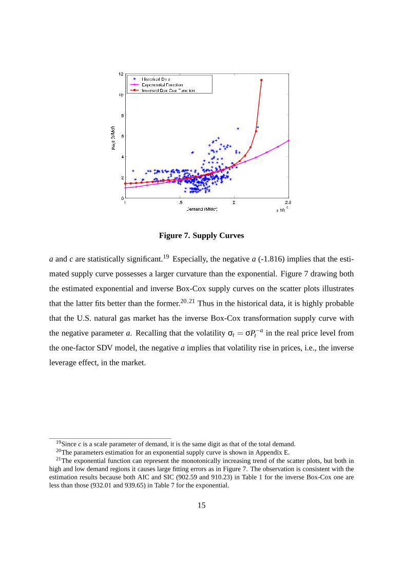
a andc are statistically significant.19 Especially, the negativea (-1.816) implies that the esti-

mated supply curve possesses a larger curvature than the exponential. Figure 7 drawing both

the estimated exponential and inverse Box-Cox supply curves on the scatter plots illustrates

that the latter fits better than the former.20,21 Thus in the historical data, it is highly probable

that the U.S. natural gas market has the inverse Box-Cox transformation supply curve with

the negative parametera. Recalling that the volatilityσt = σP−at in the real price level from

the one-factor SDV model, the negativea implies that volatility rise in prices, i.e., the inverse

leverage effect, in the market.

19Sincec is a scale parameter of demand, it is the same digit as that of the total demand.20The parameters estimation for an exponential supply curve is shown in Appendix E.21The exponential function can represent the monotonically increasing trend of the scatter plots, but both in

high and low demand regions it causes large fitting errors as in Figure 7. The observation is consistent with theestimation results because both AIC and SIC (902.59 and 910.23) in Table 1 for the inverse Box-Cox one areless than those (932.01 and 939.65) in Table 7 for the exponential.

15

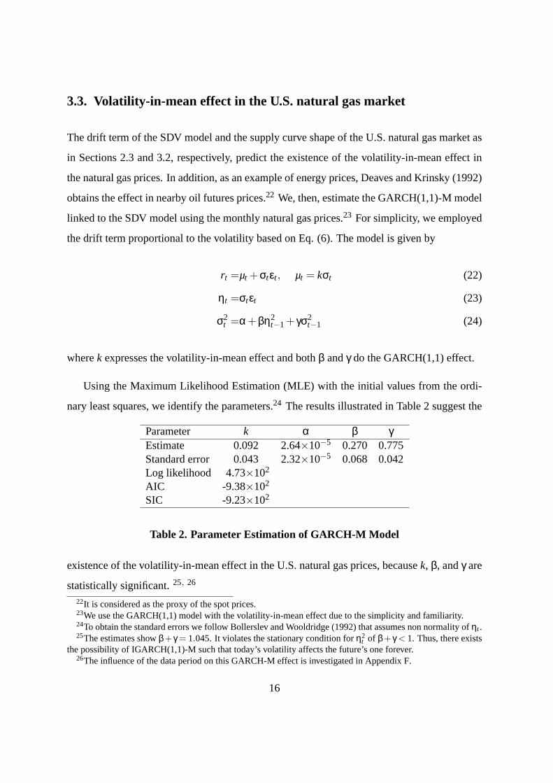
3.3. Volatility-in-mean effect in the U.S. natural gas market

The drift term of the SDV model and the supply curve shape of the U.S. natural gas market as

in Sections 2.3 and 3.2, respectively, predict the existence of the volatility-in-mean effect in

the natural gas prices. In addition, as an example of energy prices, Deaves and Krinsky (1992)

obtains the effect in nearby oil futures prices.22 We, then, estimate the GARCH(1,1)-M model

linked to the SDV model using the monthly natural gas prices.23 For simplicity, we employed

the drift term proportional to the volatility based on Eq. (6). The model is given by

rt =µt +σtεt , µt = kσt (22)

ηt =σtεt (23)

σ2t =α+βη2

t−1 + γσ2t−1 (24)

wherek expresses the volatility-in-mean effect and bothβ andγ do the GARCH(1,1) effect.

Using the Maximum Likelihood Estimation (MLE) with the initial values from the ordi-

nary least squares, we identify the parameters.24 The results illustrated in Table 2 suggest the

Parameter k α β γEstimate 0.092 2.64×10−5 0.270 0.775Standard error 0.043 2.32×10−5 0.068 0.042Log likelihood 4.73×102

AIC -9.38×102

SIC -9.23×102

Table 2. Parameter Estimation of GARCH-M Model

existence of the volatility-in-mean effect in the U.S. natural gas prices, becausek, β, andγ are

statistically significant.25, 26

22It is considered as the proxy of the spot prices.23We use the GARCH(1,1) model with the volatility-in-mean effect due to the simplicity and familiarity.24To obtain the standard errors we follow Bollerslev and Wooldridge (1992) that assumes non normality ofηt .25The estimates showβ+ γ = 1.045. It violates the stationary condition forη2

t of β+ γ < 1. Thus, there existsthe possibility of IGARCH(1,1)-M such that today’s volatility affects the future’s one forever.

26The influence of the data period on this GARCH-M effect is investigated in Appendix F.

16

4. Validity of the Assumption of Equilibrium Demand

The empirical studies in Section 3.2 substituted the sum of consumption and storage demands

for the equilibrium one. But, it is not easy to guarantee the validity of the approximation, since

the equilibrium one is not observed in the natural gas market. As a simple idea, we estimate

the inverse Box-Cox transformation parameter using an Extended Kalman Filter (EKF)27 and

then compare it with the parameter from the NLS as in Table 1.28 If both are close, we consider

that the sum may represent the equilibrium demand as the first order approximation.

The EKF is used for the parameter estimation of the supply curve function and demand

processes. Note that the improvement of the estimation accuracy introduces two factor model

for demands (Xt andYt) as in Appendix B:

dXt = (µX−λXXt)dt+σXdw1t (25)

dYt = (µY−λYYt)dt+σYdw2t (26)

Et [dw1tdw2t ] = ρwdt. (27)

Eqs. (25) and (26) are reduced to the discrete time linear models:

Xt = (1−λX∆t)Xt−1 +µX∆t +σXε1t−1≡ f1(Xt−1,Yt−1,ε1

t−1) (28)

Yt = (1−λY∆t)Yt−1 +µY∆t +σYε2t−1≡ f2(Xt−1,Yt−1,ε2

t−1) (29)

which are linear time update equations in the EKF system. Eq. (21) is the nonlinear model29:

Pt =(

1+aXt +Yt

c

) 1a

+νt ≡ h(Xt ,Yt ,νt) (30)

27Equilibrium prices and demands are observable and unobservable variables, respectively.28The NLS employs the sum of consumption and storage demands as the equilibrium demand.29We assume that seasonality can be negligible i.e.,DC

t = Xt andDSt = Yt .

17

which constitutes the nonlinear measurement equation. Following Welch and Bishop (2004),

Xt

Yt

=

Xt

Yt

+At

Xt−1− Xt−1

Yt−1−Yt−1

+Wt

ε1

t−1

ε2t−1

(31)

Pt ≈ h(Xt ,Yt ,0)+Ht

Xt − Xt

Yt −Yt

+Vtνt (32)

whereXt = f1(Xt−1,Yt−1,0), Yt = f2(Xt−1,Yt−1,0), At =

1−λX∆t 0

0 1−λY∆t

,

Wt =

σX 0

0 σY

, Ht =

(1c

(1+aXt+Yt

c

) 1a−1

1c

(1+aXt+Yt

c

) 1a−1

),

Vt = 1，V[ε1t ,ε2

t ] =

∆t ρw∆t

ρw∆t ∆t

≡Qt，andV[νt ] = m≡ Rt .

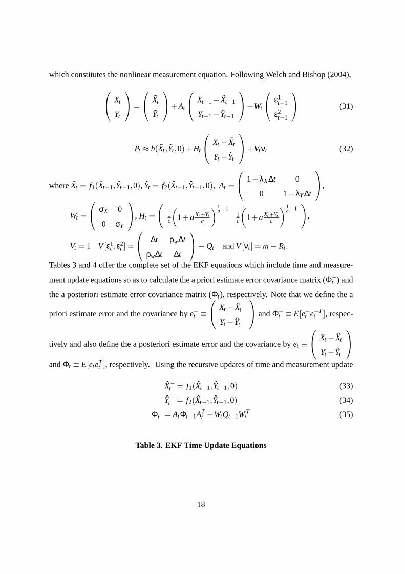
Tables 3 and 4 offer the complete set of the EKF equations which include time and measure-

ment update equations so as to calculate the a priori estimate error covariance matrix (Φ−t ) and

the a posteriori estimate error covariance matrix (Φt), respectively. Note that we define the a

priori estimate error and the covariance bye−t ≡ Xt − X−t

Yt −Y−t

andΦ−

t ≡ E[e−t e−Tt ], respec-

tively and also define the a posteriori estimate error and the covariance byet ≡ Xt − Xt

Yt −Yt

andΦt ≡ E[eteTt ], respectively. Using the recursive updates of time and measurement update

X−t = f1(Xt−1,Yt−1,0) (33)

Y−t = f2(Xt−1,Yt−1,0) (34)

Φ−t = AtΦt−1AT

t +WtQt−1WTt (35)

Table 3. EKF Time Update Equations

18

Kt = Φ−t HT

t (HtΦ−t HT

t +VtRtVTt )−1 (36)

Xt = X−t +Kt(Pt −h(X−t ,Y−t ,0)) (37)

Yt = Y−t +Kt(Pt −h(X−t ,Y−t ,0)) (38)

Φt = (I −KtHt)Φ−t (39)

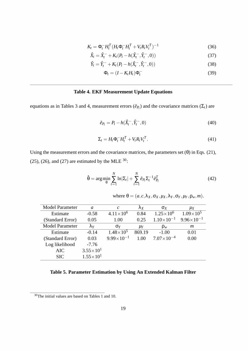
Table 4. EKF Measurement Update Equations

equations as in Tables 3 and 4, measurement errors (ePt ) and the covariance matrices (Σt) are

ePt = Pt −h(X−t ,Y−t ,0) (40)

Σt = HtΦ−t HT

t +VtRtVTt . (41)

Using the measurement errors and the covariance matrices, the parameters set (θ) in Eqs. (21),

(25), (26), and (27) are estimated by the MLE30:

θ = argminθ

N

∑t=1

ln|Σt |+N

∑t=1

ePt Σ−1t eT

Pt(42)

whereθ = (a,c,λX,σX,µX,λY,σY,µY,ρw,m).

Model Parameter a c λX σX µX

Estimate -0.58 4.11×106 0.84 1.25×106 1.09×105

(Standard Error) 0.05 1.00 0.25 1.10×10−1 9.96×10−1

Model Parameter λY σY µY ρw mEstimate -0.14 1.48×105 869.19 -1.00 0.01

(Standard Error) 0.03 9.99×10−1 1.00 7.07×10−4 0.00Log likelihood -7.76

AIC 3.55×101

SIC 1.55×101

Table 5. Parameter Estimation by Using An Extended Kalman Filter

30The initial values are based on Tables 1 and 10.

19

According to the results in Table 5, the Box-Cox transformation parameter (a) is -0.58

(negative and statistically significant), although it is a little larger than that by the demand-

price based estimation (-1.816) as in Table 1.31 In that both parameters take negative values,

we have obtained almost the same result as that in Table 1, which assumes that the sum of

consumption and storage demands represents the equilibrium demand. It indicates that the

assumption may be valid as the first order approximation.

5. Simultaneous Equations with Elastic Demand

This section investigates the validity of the demand inelasticity assumption in the SDV model

by using the natural gas data. Relaxing the assumption, we model the demand curve by the

inclined linear function, though the supply curve is the same as that in the previous sections.

The inelasticity is then examined by applying the nonlinear two-stage least square estimation

(N2SLS) in Amemiya (1974) to the simultaneous equations of the supply and demand curves.

For the identification, it is important to determine the instruments. Although the candidate

that causes the equilibrium demand fluctuation is temperature, it is known that the temperature

linearly increases in the equilibrium demand for energy. In addition, the variable at the prior

periodt−1 is often employed as the instrument for time series data, since it must be orthogonal

to model errors. Using the demand at timet − 1 as the instrument, we, then, conduct the

N2SLS estimation of the supply and demand equations.32 The model is

g1(Pt ,Dt) = Pt −(

1+aDt

c

) 1a

= εt (43)

g2(Pt ,Dt) = αPt +βDt +1 = ηt . (44)

31The inverse leverage effect is still observed, even if the equilibrium demand is assumed to be unobservable.

32Settingu1,t = εt andu2,t = ηt , we haveE[Z′tui,t ] = E

[ui,t

Dt−1ui,t

]=

[E[ui,t ]

E[Dt−1]E[ui,t ]

]=

[00

]for i = 1, 2.

As is explained in e.g., Wooldridge (2002), these instruments satisfy the efficiency condition of the N2SLS

estimation fori = 1, 2: E[u2i,tZ

′tZt ] = E

[u2

i,t

(1 Dt−1

Dt−1 D2t−1

)]= E[u2

i,t ]E[Z′tZt ].

20

Eqs. (43) and (44) represent the supply and demand curves, respectively. Ifα is not statisti-

cally significant andβ is negative and statistically significant, then the demand curve becomes

vertical implying that the demand is inelastic to the prices.

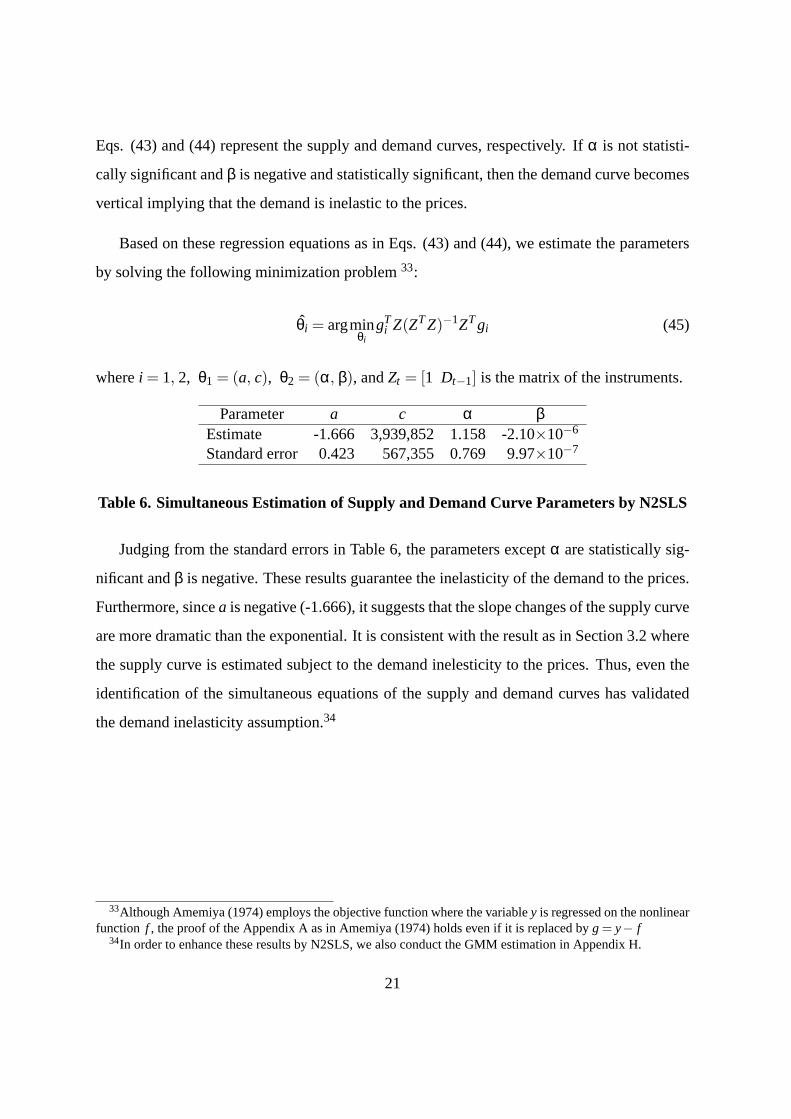
Based on these regression equations as in Eqs. (43) and (44), we estimate the parameters

by solving the following minimization problem33:

θi = argminθi

gTi Z(ZTZ)−1ZTgi (45)

wherei = 1, 2, θ1 = (a, c), θ2 = (α, β), andZt = [1 Dt−1] is the matrix of the instruments.

Parameter a c α βEstimate -1.666 3,939,852 1.158 -2.10×10−6

Standard error 0.423 567,355 0.769 9.97×10−7

Table 6. Simultaneous Estimation of Supply and Demand Curve Parameters by N2SLS

Judging from the standard errors in Table 6, the parameters exceptα are statistically sig-

nificant andβ is negative. These results guarantee the inelasticity of the demand to the prices.

Furthermore, sincea is negative (-1.666), it suggests that the slope changes of the supply curve

are more dramatic than the exponential. It is consistent with the result as in Section 3.2 where

the supply curve is estimated subject to the demand inelesticity to the prices. Thus, even the

identification of the simultaneous equations of the supply and demand curves has validated

the demand inelasticity assumption.34

33Although Amemiya (1974) employs the objective function where the variabley is regressed on the nonlinearfunction f , the proof of the Appendix A as in Amemiya (1974) holds even if it is replaced byg = y− f

34In order to enhance these results by N2SLS, we also conduct the GMM estimation in Appendix H.

21

6. Conclusions and Directions for Future Research

This paper has proposed a volatility model, which we call a Supply and Demand based Volatil-

ity (SDV) model for energy prices explicitly characterized by the supply-demand relationship.

We have illustrated that it can produce both the “time-varying volatility” and the “volatility-

in-mean effect” that characterize energy prices. Additionally, it has been shown that the SDV

model can produce the “inverse leverage effect” often seen in energy markets, supposing that

the inverse Box-Cox transformation function represents the supply curve. Moreover, this pa-

per has shown that the existing (G)ARCH-M model has foundation on the supply-demand

relationship, being derived from the discrete time SDV model with some approximation.

The empirical studies have analyzed the volatility in the U.S. natural gas prices using the

SDV model. First, we estimated the inverse Box-Cox transformation parameter representing

the supply curve curvature with the historical prices and demands. The negative estimate

implied that the natural gas prices have the inverse leverage effect: volatility increases in

prices. It is consistent with the energy market observations as in Eydeland and Wolyniec

(2003). Second, we showed that the volatility-in-mean effect is statistically significant in

GARCH(1,1)-M model. It supports the use of the volatility-in-mean models to energy prices.

Finally in order to enhance the SDV model, we have empirically examined the validity of

two model assumptions using the natural gas data. First, we have validated the assumption that

the sum of consumption and storage demands approximates to the equilibrium one by compar-

ing the inverse Box-Cox transformation parameter estimated from the extended Kalman filter

with that from the nonlinear least squares. Second, We have validated the assumption that the

demand is inelastic to the prices by conducting the identification of simultaneous equations

for the supply and demand curves with the nonlinear two-stage least square estimation.

For future research, we will conduct the empirical studies using more frequent natural gas

prices like weekly and daily ones. The applications to other energy prices like crude oil and

heating oil are possible extensions for our further studies.

22

Appendix A. Existence of Solution to One-factor SDV Model

We show the existence of the solution to the one-factor volatility model fora≤ 0 and constantµD. Eqs.

(9) - (11) are given by followings.

dPt = m(Pt)dt+s(Pt)dwt (A1)

s(x) = σ(x)x (A2)

m(x) = µ(x)x (A3)

σ(x) =

σx−a x≤ (1+aτ)1a

σ 1−a1+aτ(1+ a(1+aτ)

1a

(1−a)x ) x≥ (1+aτ)1a

(A4)

µ(x) =µD

σDσ(x)+

1−a2

σ(x)2 (A5)

Sinceσ(x) is bounded where the upper bound ofσ(x)is set askσ, we have

‖s(x)‖2 = ‖σ(x)‖2‖x‖2 ≤ k2σ(1+‖x‖2). (A6)

In addition,µ(x)is also bounded (kµ) since it is expressed by the quadratic function ofσ(x):

‖m(x)‖2 = ‖µ(x)‖2‖x‖2 ≤ k2µ(1+‖x‖2). (A7)

The results satisfy the growth condition to the coefficients (s(x) andm(x)) of the SDE (A1) (e.g., Duffie

(2001)).

Then fora≤ 0, s(x) andm(x) are continuous and differentiable with respect tox. It is verified by

the followings. Note that forx < 0 we sets(x) = 0 andm(x) = 0.

limx→+0

∂s(x)∂x

= limx→+0

(−a+1)σx−a = 0 (A8)

limx→(1+aτ)

1a

∂s(x)∂x

= σ1−a1+aτ

(A9)

limx→+∞

∂s(x)∂x

= σ1−a1+aτ

(A10)

23

limx→+0

∂m(x)∂x

= limx→+0

(−a+1)µD

σDσx−a +

1−a2

(−2a+1)σ2x−2a = 0 (A11)

limx→(1+aτ)

1a

∂m(x)∂x

=µD

σDσ

1−a1+aτ

+(1−a)(1−2a)

2σ2

(1+aτ)2 (A12)

limx→+∞

∂m(x)∂x

=µD

σDσ

1−a1+aτ

+1−a

2σ2

(1−a1+aτ

)2

(A13)

The results satisfy the Lipschitz condition to the coefficientss(x) andm(x) as in SDE (A1). In conclu-

sion, it suggests that the one-factor SDV model as in Eq. (A1) has a unique strong solution.

Appendix B. Two-factor SDV Model

We formulate the two-factor SDV model that incorporates consumption and storage demands. Denoting

by DCt consumption demand for energy, the deviation (Xt) from the average demand (DC

t ) is assumed

to follow a mean reverting process, as is often observed in energy markets.35

DCt = Xt + DC

t (B14)

dXt = (µX−λXXt)dt+σXdw1t . (B15)

Then, we introduce the storage demand (DS) which is also divided into the mean reverting deviation

process (Yt) and the average (DSt). The decomposition expresses the seasonal pattern and the deviation

of storage demand. The storage demand model is given by

DSt = Yt + DS

t (B16)

dYt = (µY−λYYt)dt+σYdw2t . (B17)

The mean reversion reflects the characteristic of storage such that the deviation is expected to reach a

certain level in a long run if it is far from the level.

35As is in one-factor model, the mean reversion of consumption demand reflects that of temperature, since itis often modeled by a mean reverting process.

24

In order to obtain the prices, we use a supply-demand relationship where we assume that the de-

mand curve is vertical and the supply curve is an inverse Box-Cox transformation function. The equi-

librium prices are recovered from the supply curve, substituting the demand for the supply

Pt =

(1+aXt+Yt+ f (t)−b

c

) 1a

(Xt +Yt + f (t)−b≤ cτ)

(1+aτ)1a

1−a

[exp

(1−a1+aτ

(Xt+Yt+ f (t)−b

c − τ))

−a

](Xt +Yt + f (t)−b≥ cτ)

(B18)

where f (t) denotes the sum ofDCt and DS

t . We define byZ and qt as follows: Zt = Xt+Yt+ f (t)−bc ,

qt = 1c

(1− λY

λX

)Yt . Applying Ito’s Lemma to Eq. (B18) by using Eqs. (B15) and (B17), the two-factor

SDV model for energy prices is expressed by followings36:

dPt

Pt= µtdt+σtdwt (B19)

dZt = {µZ +λX(qt −Zt)− 12

σ2Z}dt+σZdwt (B20)

dqt = (µq−λYqt)dt+σqdw2t (B21)

σt =

σZP−at Pt ≤ (1+aτ)

1a

σZ1−a1+aτ(1+ a(1+aτ)

1a

(1−a)Pt) Pt ≥ (1+aτ)

1a

(B22)

µt =12(1−a)σ2

t +(

1σZ

(µZ− 12

σ2Z)+

λX

σZ(qt −Zt)

)σt (B23)

Et [dwtdw2t ] = γdt (B24)

µZ =1c( f ′(t)+µX +µY +λX( f (t)−b))+

12

σ2Z (B25)

σZ =1c

√σ2

X +σ2Y +2ρwσXσY (B26)

where dwt = 1cσZ

(σXdw1t +σYdw2t), µq = λX−λYcλX

µY, σq = λX−λYcλX

σY, and γ = σXρw+σYσZ

.

We find that, like the one-factor SDV model, the two-factor SDV model is also classified in the

C.E.V. models, judging from the volatility in Eq. (B22) forPt ≤ (1+aτ)1a . The drift term in Eq. (B23)

stems from the volatility. It leads to the volatility-in-mean model.

36We employ Eq. (B23) in order that the two-factor SDV model is consistent with the one-factor SDV modelalthough Eq.(B23) is different from that obtained by the supply curve in the supply region more thancτ.

25

Appendix C. Proof of Proposition 2

Employing the Taylor expansion with respect toDt around 0 for Eq. (13), we have

σ2t =

σ2D

c2

(1+

∞

∑k=1

(−1)k(k+1)(

ac

)k

Dkt

). (C27)

We assume that the demand process follows AR(1) model:

Dt = (1−λD)Dt−1 +µD +σDεt−1. (C28)

It is reduced to

Dt = (1−λD)tD0 +µD

λD{1− (1−λD)t}+σD

t

∑i=1

(1−λD)i−1εt−i . (C29)

We setMt = (1−λD)tD0+ µDλD{1− (1−λD)t} andki = σD(1−λD)i−1. Substituting Eq. (C29) into Eq.

(C27), we obtain Eq. (18). We, then, have Eqs. from (16) to (18) as the discrete time SDV model.

If the past demand shocks and the squares dominate the volatility,εkε j = 0 holds fork 6= j. We,

then, writeDt to the power ofn as:

Dnt ≈

n

∑j=0

t

∑i=1

a j,i,nεn− jt−i (C30)

wherea j,i,n = nCjMjt kn− j

i ( j 6= n) anda j,i,n = 1t Mn

t ( j = n). Injecting Eq. (C30) into Eq. (C27), we have

σ2t ≈

σ2D

c2

∞

∑k=0

t

∑i=1

αi,kεkt−i (C31)

whereαi,k = ∑∞l=k(−1)l (l + 1)(a

c)l al−k,i,l . Expressingσt by Dt from Eq. (13) and employing the

definition ofηt , we have

εt =

(c+aDt

σD

)ηt . (C32)

Notice that

Dt = Mt +t

∑j=1

k jεt− j . (C33)

26

Substituting Eqs. (C32) and (C33) into Eq. (C31), we have

σ2t ≈

σ2D

c2

∞

∑k=0

t

∑i=1

αi,k

(c+aMt−i +a∑t−i

j=1k jεt−i− j

σD

)k

ηkt−i . (C34)

Remind that by definitionηt−i is expressed byεt−i and thatεkε j = 0 for k 6= j when the past demand

shocks and the squares dominate the volatility, we have

σ2t ≈

σ2D

c2

∞

∑k=0

t

∑i=1

Ai,kηkt−i (C35)

whereAi,k = αi,kbi,k andbi,k =(c+aMt−i

σD

)k. If the squares of the past demand shocks only dominate the

volatility, we have Eq. (19).‖

Appendix D. Proof of Corollary 1

The mean reversion of the demand process whose implication is0≤ 1−λD ≤ 1 causes positiveki . It

also causes the positive and constant long term average ofMt represented byµDλD

. These positives ofki

andMt lead to positiveal−k,i,l as in Eq. (20). Additionallybi,k, c, and−a are all positive by definition.

These results lead to positiveAi,k.‖

Appendix E. Exponential Supply Curve Parameters

We model the supply curve in the U.S. natural gas market usingPt = eSt−b

c . Since the supply is equiva-

lent to the sum of consumption and storage demands in equilibrium, we haveSt = DCt +DS

t . Substituting

it into the exponential function, we have

Pt = eDC

t +DSt −b

c . (E36)

We estimate bothb andc in Eq. (E36) by using the NLS. The results are illustrated in Table 7. Judging

from thet-statistics as in Table 7, both parameters are statistically significant.

27

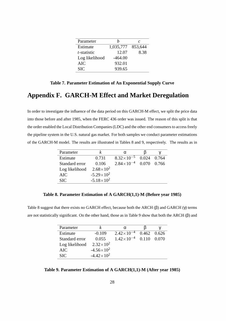
Parameter b cEstimate 1,035,777 853,644t-statistic 12.07 8.38Log likelihood -464.00AIC 932.01SIC 939.65

Table 7. Parameter Estimation of An Exponential Supply Curve

Appendix F. GARCH-M Effect and Market Deregulation

In order to investigate the influence of the data period on this GARCH-M effect, we split the price data

into those before and after 1985, when the FERC 436 order was issued. The reason of this split is that

the order enabled the Local Distribution Companies (LDC) and the other end consumers to access freely

the pipeline system in the U.S. natural gas market. For both samples we conduct parameter estimations

of the GARCH-M model. The results are illustrated in Tables 8 and 9, respectively. The results as in

Parameter k α β γEstimate 0.731 8.32×10−5 0.024 0.764Standard error 0.106 2.84×10−4 0.070 0.766Log likelihood 2.68×102

AIC -5.29×102

SIC -5.18×102

Table 8. Parameter Estimation of A GARCH(1,1)-M (Before year 1985)

Table 8 suggest that there exists no GARCH effect, because both the ARCH (β) and GARCH (γ) terms

are not statistically significant. On the other hand, those as in Table 9 show that both the ARCH (β) and

Parameter k α β γEstimate -0.109 2.42×10−4 0.462 0.626Standard error 0.055 1.42×10−4 0.110 0.070Log likelihood 2.32×102

AIC -4.56×102

SIC -4.42×102

Table 9. Parameter Estimation of A GARCH(1,1)-M (After year 1985)

28

GARCH (γ) terms and volatility-in-mean term (k) are all statistically significant. The estimation results

imply that the GARCH-M effect in the whole data set arises from that after 1985, when the market is

partly deregulated by the FERC 436 order.

Appendix G. Parameter Estimation of Demand Processes

We calibrate the consumption and storage demand models in Appendix B to the historical data. Since

the corresponding deviations are Eqs. (B15) and (B17), respectively, the discrete time models are

Xt+1 = cX +ρXXt + εX. (G37)

Yt+1 = cY +ρYYt + εY (G38)

whereε = (εX,εY)′ ∼ N(µ,Σ), µ= (0,0)′, andΣ =

θ2

X γXYθXθY

γXYθXθY θ2Y

. The MLE is applied to

the models using the initial values from the least squares for each process.

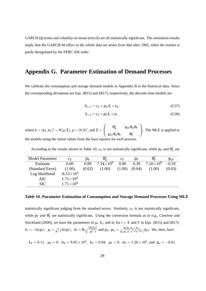
According to the results shown in Table 10,cX is not statistically significant, whileρX andθ2X are

Model Parameter cX ρX θ2X cY ρY θ2

Y γXY

Estimate 0.00 0.89 7.34×109 0.00 0.39 7.10×109 -0.59(Standard Error) (1.00) (0.02) (1.00) (1.00) (0.04) (1.00) (0.03)Log likelihood -8.53×103

AIC 1.71×104

SIC 1.71×104

Table 10. Parameter Estimation of Consumption and Storage Demand Processes Using MLE

statistically significant judging from the standard errors. Similarly,cY is not statistically significant,

while ρY andθ2Y are statistically significant. Using the conversion formula as in e.g., Clewlow and

Strickland (2000), we have the parameters ofµi , λi , andσi for i = X andY in Eqs. (B15) and (B17):

λi =−ln(ρi), µi = ciρi−1 ln(ρi), σi = θi

√2ln(ρi)ρ2

i −1andρw: ρw = θXθY(λX+λY)

σXσY(1−e−(λX+λY))γXY. We, then, have

λX = 0.11, µX = 0, σX = 9.05×104, λY = 0.94, µY = 0, σY = 1.26×105, and ρw =−0.61.

29

The estimates indicate that the long term averages of bothXt andYt are zero due to insignificance of

cX andcY. In addition, since the parameters for the two-factor model are significant besidesµX andµY,

consumption and storage demands may be justified in employing the mean reverting processes.

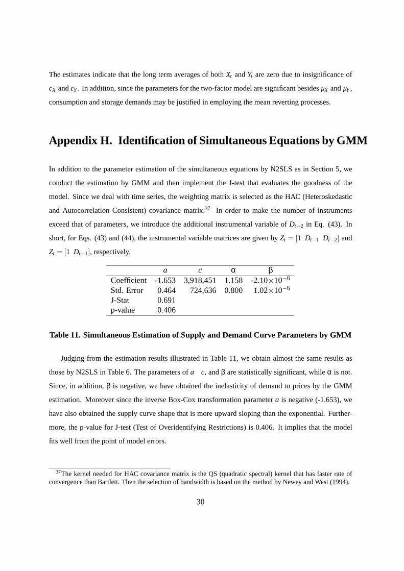
Appendix H. Identification of Simultaneous Equations by GMM

In addition to the parameter estimation of the simultaneous equations by N2SLS as in Section 5, we

conduct the estimation by GMM and then implement the J-test that evaluates the goodness of the

model. Since we deal with time series, the weighting matrix is selected as the HAC (Heteroskedastic

and Autocorrelation Consistent) covariance matrix.37 In order to make the number of instruments

exceed that of parameters, we introduce the additional instrumental variable ofDt−2 in Eq. (43). In

short, for Eqs. (43) and (44), the instrumental variable matrices are given byZt = [1 Dt−1 Dt−2] and

Zt = [1 Dt−1], respectively.

a c α βCoefficient -1.653 3,918,451 1.158 -2.10×10−6

Std. Error 0.464 724,636 0.800 1.02×10−6

J-Stat 0.691p-value 0.406

Table 11. Simultaneous Estimation of Supply and Demand Curve Parameters by GMM

Judging from the estimation results illustrated in Table 11, we obtain almost the same results as

those by N2SLS in Table 6. The parameters ofa，c, andβ are statistically significant, whileα is not.

Since, in addition,β is negative, we have obtained the inelasticity of demand to prices by the GMM

estimation. Moreover since the inverse Box-Cox transformation parametera is negative (-1.653), we

have also obtained the supply curve shape that is more upward sloping than the exponential. Further-

more, the p-value for J-test (Test of Overidentifying Restrictions) is 0.406. It implies that the model

fits well from the point of model errors.

37The kernel needed for HAC covariance matrix is the QS (quadratic spectral) kernel that has faster rate ofconvergence than Bartlett. Then the selection of bandwidth is based on the method by Newey and West (1994).

30

References

Amemiya, T., 1974, The Nonlinear Two-Stage Least-Squares Estimator,Journal of Econometrics2,

105–110.

Barlow, M. T., 2002, A Diffusion Model for Electricity Prices,Mathematical Finance12, 287–298.

Bollerslev, T., 1986, Generalized Autoregressive Conditional Heteroskedasticity,Journal of Economet-

rics 31, 307–327.

Bollerslev, T., and J. M. Wooldridge, 1992, Quasi-Maximum Likelihood Estimation and Inference in

Dynamic Models with Time Varying Covariances,Econometric Reviews11, 143–172.

Clewlow, L., and C. Strickland, 2000,Energy Derivatives: Pricing and Risk Management. (Lacima

Publications London).

Cox, J., 1975, Notes on Option Pricing I: Constant Elasticity of Variance Diffusions, Working paper,

Stanford University (reprinted inJournal of Portfolio Management, 1996, 22 15-17).

Deaves, R., and I. Krinsky, 1992, Risk Premiums and Efficiency in the Market for Crude Oil Futures,

The Energy Journal13, 93–117.

Duffie, D., 2001,Dynamic Asset Pricing Theory, Third Edition. (Princeton University Press New Jer-

sey).

Duffie, D., S. Gray, and P. Hoang, 1999, Volatility in Energy Prices, in Vincent Kaminski, eds.:MAN-

AGING ENERGY PRICE RISK(RISK PUBLICATIONS, London ).

Emanuel, D., and J. MacBeth, 1982, Further Results on the Constant Elasticity of Variance Call Option

Pricing Model,Journal of Financial and Quantitative Analysis17, 533–554.

Engle, R., 1982, Autoregressive Conditional Heteroscedasticity with Estimates of the Variance of

United Kingdom Inflation,Econometrica50, 987–1007.

Engle, R., D. Lilien, and R. Robins, 1987, Estimating Time Varying Risk Premia in the Term Structure:

The Arch-M Model,Econometrica55, 391–407.

31

Eydeland, A., and K. Wolyniec, 2003,Energy and Power Risk Management: New Developments in

Modeling, Pricing, and Hedging. (John Wiley& Sons, Inc. Hoboken).

Heston, S., 1993, A Closed-Form Solution for Options with Stochastic Volatility with Applications to

Bond and Currency Options,The Review of Financial Studies6, 327–343.

Kanamura, T., and K.Ohashi, 2006, A Structural Model for Electricity Prices with Spikes: Mea-

surement of Spike Risk and Optimal Policies for Hydropower Plant Operation,Energy Economics,

forthcoming.

Newey, W. K., and K. D. West, 1994, Automatic Lag Selection in Covariance Matrix Estimation,

Review of Economic Studies61, 631–653.

Pindyck, R. S., 2004, Volatility in Natural Gas and Oil Markets, Working paper, Massachusetts Institute

of Technology.

Welch, G., and G. Bishop, 2004, An Introduction to the Kalman Filter, Working paper, University of

North Carolina at Chapel Hill.

Wooldridge, J. M., 2002,Econometric Analysis of Cross Section and Panel Data. (The MIT Press

Cambridge).

32