Embed Size (px)
Citation preview
PUB. IRMA, LILLE 2009Vol. 69, No VII
A survey of cross-validation procedures for modelselection ∗
Sylvain Arlot,CNRS ; Willow Project-Team,
Laboratoire d’Informatique de l’École Normale Supérieure
(CNRS/ENS/INRIA UMR 8548)
45, rue d’Ulm, 75 230 Paris, France
Alain Celisse,Laboratoire Paul Painlevé, UMR CNRS 8524,
Université des Sciences et Technologies de Lille 1
F-59 655 Villeneuve d’Ascq Cedex, France
Abstract
Used to estimate the risk of an estimator or to perform model selec-tion, cross-validation is a widespread strategy because of its simplicityand its apparent universality. Many results exist on the model selectionperformances of cross-validation procedures. This survey intends to relatethese results to the most recent advances of model selection theory, with aparticular emphasis on distinguishing empirical statements from rigoroustheoretical results. As a conclusion, guidelines are provided for choosingthe best cross-validation procedure according to the particular features ofthe problem in hand.
Résumé
La validation-croisée est une technique d’estimation de risque ou de sé-lection de modèle très répandue du fait de sa simplicité et de son caractèreuniversel. De nombreux résultats existent concernant les performances dela validation-croisée en sélection de modèle. L’objectif de ce travail et desynthétiser ces résultats ainsi que les avancées les plus récentes de la théo-rie de la sélection de modèle. Une attention toute particulière est portéesur la distinction entre résultats théoriques rigoureux et considérationsempiriques. En guise de conclusion, des indications sont fournies afin dechoisir la technique de validation-croisée la plus appropriée aux particu-larités du problème considéré.
∗Preprint.

VII – 3
Keywords. cross-validation, leave-p-out, leave-one-out, V-fold cross-validation,risk estimation, model selection, efficiency, model consistency.MSC classifications: 62-02 ; 62G09 ; 62G08 ; 62G05.
VII – 4
Contents1 Introduction 5
1.1 Statistical framework . . . . . . . . . . . . . . . . . . . . . . . . . 61.2 Examples . . . . . . . . . . . . . . . . . . . . . . . . . . . . . . . 71.3 Statistical algorithms . . . . . . . . . . . . . . . . . . . . . . . . . 8
2 Model selection 92.1 The model selection paradigm . . . . . . . . . . . . . . . . . . . . 92.2 Model selection for estimation . . . . . . . . . . . . . . . . . . . . 102.3 Model selection for identification . . . . . . . . . . . . . . . . . . 112.4 Estimation vs. identification . . . . . . . . . . . . . . . . . . . . . 11
3 Overview of some model selection procedures 113.1 The unbiased risk estimation principle . . . . . . . . . . . . . . . 123.2 Biased estimation of the risk . . . . . . . . . . . . . . . . . . . . 133.3 Procedures built for identification . . . . . . . . . . . . . . . . . . 143.4 Structural risk minimization . . . . . . . . . . . . . . . . . . . . . 143.5 Ad hoc penalization . . . . . . . . . . . . . . . . . . . . . . . . . . 153.6 Where are cross-validation procedures in this picture? . . . . . . 15
4 Cross-validation procedures 164.1 Cross-validation philosophy . . . . . . . . . . . . . . . . . . . . . 164.2 From validation to cross-validation . . . . . . . . . . . . . . . . . 16
4.2.1 Hold-out . . . . . . . . . . . . . . . . . . . . . . . . . . . . 164.2.2 General definition of cross-validation . . . . . . . . . . . . 17
4.3 Classical examples . . . . . . . . . . . . . . . . . . . . . . . . . . 174.3.1 Exhaustive data splitting . . . . . . . . . . . . . . . . . . 184.3.2 Partial data splitting . . . . . . . . . . . . . . . . . . . . . 184.3.3 Other cross-validation-like risk estimators . . . . . . . . . 19
4.4 Historical remarks . . . . . . . . . . . . . . . . . . . . . . . . . . 20
5 Statistical properties of cross-validation estimators of the risk 215.1 Bias . . . . . . . . . . . . . . . . . . . . . . . . . . . . . . . . . . 21
5.1.1 Theoretical assessment of the bias . . . . . . . . . . . . . 215.1.2 Correction of the bias . . . . . . . . . . . . . . . . . . . . 22
5.2 Variance . . . . . . . . . . . . . . . . . . . . . . . . . . . . . . . . 235.2.1 Variability factors . . . . . . . . . . . . . . . . . . . . . . 235.2.2 Theoretical assessment of the variance . . . . . . . . . . . 245.2.3 Estimation of the variance . . . . . . . . . . . . . . . . . . 25
6 Cross-validation for efficient model selection 266.1 Relationship between risk estimation and model selection . . . . 266.2 The global picture . . . . . . . . . . . . . . . . . . . . . . . . . . 266.3 Results in various frameworks . . . . . . . . . . . . . . . . . . . . 27
VII – 5
7 Cross-validation for identification 297.1 General conditions towards model consistency . . . . . . . . . . . 297.2 Refined analysis for the algorithm selection problem . . . . . . . 30
8 Specificities of some frameworks 318.1 Density estimation . . . . . . . . . . . . . . . . . . . . . . . . . . 318.2 Robustness to outliers . . . . . . . . . . . . . . . . . . . . . . . . 318.3 Time series and dependent observations . . . . . . . . . . . . . . 318.4 Large number of models . . . . . . . . . . . . . . . . . . . . . . . 33
9 Closed-form formulas and fast computation 33
10 Conclusion: which cross-validation method for which problem? 3410.1 The general picture . . . . . . . . . . . . . . . . . . . . . . . . . . 3410.2 How the splits should be chosen? . . . . . . . . . . . . . . . . . . 3510.3 V-fold cross-validation . . . . . . . . . . . . . . . . . . . . . . . . 3610.4 Future research . . . . . . . . . . . . . . . . . . . . . . . . . . . . 37
1 IntroductionMany statistical algorithms, such as likelihood maximization, least squares andempirical contrast minimization, rely on the preliminary choice of a model, thatis of a set of parameters from which an estimate will be returned. When severalcandidate models (thus algorithms) are available, choosing one of them is calledthe model selection problem.
Cross-validation (CV) is a popular strategy for model selection, and moregenerally algorithm selection. The main idea behind CV is to split the data (onceor several times) for estimating the risk of each algorithm: Part of the data (thetraining sample) is used for training each algorithm, and the remaining part(the validation sample) is used for estimating the risk of the algorithm. Then,CV selects the algorithm with the smallest estimated risk.
Compared to the resubstitution error, CV avoids overfitting because thetraining sample is independent from the validation sample (at least when dataare i.i.d.). The popularity of CV mostly comes from the generality of the datasplitting heuristics, which only assumes that data are i.i.d.. Nevertheless, the-oretical and empirical studies of CV procedures do not entirely confirm this“universality”. Some CV procedures have been proved to fail for some modelselection problems, depending on the goal of model selection: estimation oridentification (see Section 2). Furthermore, many theoretical questions aboutCV remain widely open.
The aim of the present survey is to provide a clear picture of what is knownabout CV, from both theoretical and empirical points of view. More precisely,the aim is to answer the following questions: What is CV doing? When doesCV work for model selection, keeping in mind that model selection can target
VII – 6
different goals? Which CV procedure should be used for each model selectionproblem?
The paper is organized as follows. First, the rest of Section 1 presents thestatistical framework. Although non exhaustive, the present setting has beenchosen general enough for sketching the complexity of CV for model selection.The model selection problem is introduced in Section 2. A brief overview ofsome model selection procedures that are important to keep in mind for un-derstanding CV is given in Section 3. The most classical CV procedures aredefined in Section 4. Since they are the keystone of the behaviour of CV formodel selection, the main properties of CV estimators of the risk for a fixedmodel are detailed in Section 5. Then, the general performances of CV formodel selection are described, when the goal is either estimation (Section 6) oridentification (Section 7). Specific properties of CV in some particular frame-works are discussed in Section 8. Finally, Section 9 focuses on the algorithmiccomplexity of CV procedures, and Section 10 concludes the survey by tacklingseveral practical questions about CV.
1.1 Statistical frameworkAssume that some data ξ1, . . . , ξn ∈ Ξ with common distribution P are ob-served. Throughout the paper—except in Section 8.3—the ξi are assumed tobe independent. The purpose of statistical inference is to estimate from thedata (ξi )1≤i≤n some target feature s of the unknown distribution P , such asthe mean or the variance of P . Let S denote the set of possible values for s.The quality of t ∈ S, as an approximation of s, is measured by its loss L ( t ),where L : S 7→ R is called the loss function, and is assumed to be minimal fort = s. Many loss functions can be chosen for a given statistical problem.
Several classical loss functions are defined by
L ( t ) = LP ( t ) := Eξ∼P [γ ( t; ξ ) ] , (1)
where γ : S × Ξ 7→ [0,∞) is called a contrast function. Basically, for t ∈ Sand ξ ∈ Ξ, γ(t; ξ) measures how well t is in accordance with observation of ξ,so that the loss of t, defined by (1), measures the average accordance betweent and new observations ξ with distribution P . Therefore, several frameworkssuch as transductive learning do not fit definition (1). Nevertheless, as detailedin Section 1.2, definition (1) includes most classical statistical frameworks.
Another useful quantity is the excess loss
` (s, t ) := LP ( t )− LP (s ) ≥ 0 ,
which is related to the risk of an estimator s of the target s by
R( s ) = Eξ1,...,ξn∼P [` (s, s ) ] .
VII – 7
1.2 ExamplesThe purpose of this subsection is to show that the framework of Section 1.1includes several important statistical frameworks. This list of examples doesnot pretend to be exhaustive.
Density estimation aims at estimating the density s of P with respect tosome given measure µ on Ξ. Then, S is the set of densities on Ξ with respectto µ. For instance, taking γ(t;x) = − ln(t(x)) in (1), the loss is minimal whent = s and the excess loss
` (s, t ) = LP ( t )− LP (s ) = Eξ∼P
[ln
(s(ξ)t(ξ)
)]=
∫s ln
( s
t
)dµ
is the Kullback-Leibler divergence between distributions tµ and sµ.
Prediction aims at predicting a quantity of interest Y ∈ Y given an explana-tory variable X ∈ X and a sample of observations (X1, Y1), . . . , (Xn, Yn). Inother words, Ξ = X × Y, S is the set of measurable mappings X 7→ Y and thecontrast γ(t; (x, y)) measures the discrepancy between the observed y and itspredicted value t(x). Two classical prediction frameworks are regression andclassification, which are detailed below.
Regression corresponds to continuous Y, that is Y ⊂ R (or Rk for multivari-ate regression), the feature space X being typically a subset of R`. Let s denotethe regression function, that is s(x) = E(X,Y )∼P [Y | X = x ], so that
∀i, Yi = s(Xi) + εi with E [εi | Xi ] = 0 .
A popular contrast in regression is the least-squares contrast γ ( t; (x, y) ) =(t(x)− y)2, which is minimal over S for t = s, and the excess loss is
` (s, t ) = E(X,Y )∼P
[(s(X)− t(X) )2
].
Note that the excess loss of t is the square of the L2 distance between t and s,so that prediction and estimation are equivalent goals.
Classification corresponds to finite Y (at least discrete). In particular, whenY = {0, 1}, the prediction problem is called binary (supervised) classification.With the 0-1 contrast function γ(t; (x, y)) = 1lt(x) 6=y, the minimizer of the lossis the so-called Bayes classifier s defined by
s(x) = 1lη(x)≥1/2 ,
where η denotes the regression function η(x) = P(X,Y )∼P (Y = 1 | X = x ).Remark that a slightly different framework is often considered in binary clas-
sification. Instead of looking only for a classifier, the goal is to estimate also the
VII – 8
confidence in the classification made at each point: S is the set of measurablemappings X 7→ R, the classifier x 7→ 1lt(x)≥0 being associated to any t ∈ S.Basically, the larger |t(x)|, the more confident we are in the classification madefrom t(x). A classical family of losses associated with this problem is defined by(1) with the contrast γφ ( t; (x, y) ) = φ (−(2y − 1)t(x) ) where φ : R 7→ [0,∞)is some function. The 0-1 contrast corresponds to φ(u) = 1lu≥0. The convexloss functions correspond to the case where φ is convex, nondecreasing withlim−∞ φ = 0 and φ(0) = 1. Classical examples are φ(u) = max {1 + u, 0}(hinge), φ(u) = exp(u), and φ(u) = log2 (1 + exp(u) ) (logit). The correspond-ing losses are used as objective functions by several classical learning algorithmssuch as support vector machines (hinge) and boosting (exponential and logit).
Many references on classification theory, including model selection, can befound in the survey by Boucheron et al. (2005).
1.3 Statistical algorithmsIn this survey, a statistical algorithm A is any (measurable) mapping A :⋃
n∈N Ξn 7→ S. The idea is that data Dn = (ξi )1≤i≤n ∈ Ξn will be used asan input of A, and that the output of A, A(Dn) = sA(Dn) ∈ S, is an estimatorof s. The quality of A is then measured by LP
(sA(Dn)
), which should be as
small as possible. In the sequel, the algorithm A and the estimator sA(Dn) areoften identified when no confusion is possible.
Minimum contrast estimators form a classical family of statistical algorithms,defined as follows. Given some subset S of S that we call a model, a minimumcontrast estimator of s is any minimizer of the empirical contrast
t 7→ LPn( t ) =
1n
n∑i=1
γ ( t; ξi ) , where Pn =1n
n∑i=1
δξi ,
over S. The idea is that the empirical contrast LPn ( t ) has an expectationLP ( t ) which is minimal over S at s. Hence, minimizing LPn ( t ) over a set S ofcandidate values for s hopefully leads to a good estimator of s. Let us now givethree popular examples of empirical contrast minimizers:
• Maximum likelihood estimators: take γ(t;x) = − ln(t(x)) in the densityestimation setting. A classical choice for S is the set of piecewise constantfunctions on a regular partition of Ξ with K pieces.
• Least-squares estimators: take γ(t; (x, y)) = (t(x) − y)2 the least-squarescontrast in the regression setting. For instance, S can be the set of piece-wise constant functions on some fixed partition of X (leading to regresso-grams), or a vector space spanned by the first vectors of wavelets or Fourierbasis, among many others. Note that regularized least-squares algorithmssuch as the Lasso, ridge regression and spline smoothing also are least-squares estimators, the model S being some ball of a (data-dependent)radius for the L1 (resp. L2) norm in some high-dimensional space. Hence,
VII – 9
tuning the regularization parameter for the LASSO or SVM, for instance,amounts to perform model selection from a collection of models.
• Empirical risk minimizers, following the terminology of Vapnik (1982):take any contrast function γ in the prediction setting. When γ is the 0-1contrast, popular choices for S lead to linear classifiers, partitioning rules,and neural networks. Boosting and Support Vector Machines classifiersalso are empirical contrast minimizers over some data-dependent modelS, with contrast γ = γφ for some convex functions φ.
Let us finally mention that many other classical statistical algorithms canbe considered with CV, for instance local average estimators in the predictionframework such as k-Nearest Neighbours and Nadaraya-Watson kernel estima-tors. The focus will be mainly kept on minimum contrast estimators to keepthe length of the survey reasonable.
2 Model selectionUsually, several statistical algorithms can be used for solving a given statisticalproblem. Let ( sλ )λ∈Λ denote such a family of candidate statistical algorithms.The algorithm selection problem aims at choosing from data one of these algo-rithms, that is, choosing some λ(Dn) ∈ Λ. Then, the final estimator of s is givenby sbλ(Dn)(Dn). The main difficulty is that the same data are used for training
the algorithms, that is, for computing ( sλ(Dn) )λ∈Λ, and for choosing λ(Dn) .
2.1 The model selection paradigmFollowing Section 1.3, let us focus on the model selection problem, where can-didate algorithms are minimum contrast estimators and the goal is to choose amodel S. Let (Sm )m∈Mn
be a family of models, that is, Sm ⊂ S. Let γ be afixed contrast function, and for every m ∈ Mn, let sm be a minimum contrastestimator over model Sm with contrast γ. The goal is to choose m(Dn) ∈ Mn
from data only.
The choice of a model Sm has to be done carefully. Indeed, when Sm is a“small” model, sm is a poor statistical algorithm except when s is very close toSm, since
` (s, sm ) ≥ inft∈Sm
{` (s, t )} := ` (s, Sm ) .
The lower bound ` (s, Sm ) is called the bias of model Sm, or approximationerror. The bias is a nonincreasing function of Sm.
On the contrary, when Sm is “huge”, its bias ` (s, Sm ) is small for mosttargets s, but sm clearly overfits. Think for instance of Sm as the set of allcontinuous functions on [0, 1] in the regression framework. More generally, ifSm is a vector space of dimension Dm, in several classical frameworks,
E [` (s, sm(Dn) ) ] ≈ ` (s, Sm ) + λDm (2)
VII – 10
where λ > 0 does not depend on m. For instance, λ = 1/(2n) in densityestimation using the likelihood contrast, and λ = σ2/n in regression using theleast-squares contrast and assuming var (Y | X ) = σ2 does not depend on X.The meaning of (2) is that a good model choice should balance the bias term` (s, Sm ) and the variance term λDm, that is solve the so-called bias-variancetrade-off. By extension, the variance term, also called estimation error, can bedefined by
E [` (s, sm(Dn) ) ]− ` (s, Sm ) = E [LP ( sm ) ]− inft∈Sm
LP ( t ) ,
even when (2) does not hold.The interested reader can find a much deeper insight into model selection in
the Saint-Flour lecture notes by Massart (2007).
Before giving examples of classical model selection procedures, let us mentionthe two main different goals that model selection can target: estimation andidentification.
2.2 Model selection for estimationOn the one hand, the goal of model selection is estimation when s bm(Dn)(Dn)is used as an approximation of the target s, and the goal is to minimize itsloss. For instance, AIC and Mallows’ Cp model selection procedures are builtfor estimation (see Section 3.1).
The quality of a model selection procedure Dn 7→ m(Dn), designed for esti-mation, is measured by the excess loss of s bm(Dn)(Dn). Hence, the best possiblemodel choice for estimation is the so-called oracle model Sm? , defined by
m? = m?(Dn) ∈ arg minm∈Mn
{` (s, sm(Dn) )} . (3)
Since m?(Dn) depends on the unknown distribution P of data, one cannotexpect to select m(Dn) = m?(Dn) almost surely. Nevertheless, we can hope toselect m(Dn) such that s bm(Dn) is almost as close to s as s m?(Dn). Note thatthere is no requirement for s to belong to
⋃m∈Mn
Sm.
Depending on the framework, the optimality of a model selection procedurefor estimation is assessed in at least two different ways.
First, in the asymptotic framework, a model selection procedure m is calledefficient (or asymptotically optimal) when it leads to m such that
`(s, s bm(Dn)(Dn)
)infm∈Mn
{` (s, sm(Dn) )}a.s.−−−−→
n→∞1 .
Sometimes, a weaker result is proved, the convergence holding only in probabil-ity.
Second, in the non-asymptotic framework, a model selection procedure sat-isfies an oracle inequality with constant Cn ≥ 1 and remainder term Rn ≥ 0when
`(s, s bm(Dn)(Dn)
)≤ Cn inf
m∈Mn
{` (s, sm(Dn) )}+ Rn (4)
VII – 11
holds either in expectation or with large probability (that is, a probability largerthan 1 − C ′/n2, for some positive constant C ′). Note that if (4) holds ona large probability event with Cn tending to 1 when n tends to infinity andRn � ` (s, sm?(Dn) ), then the model selection procedure m is efficient.
In the estimation setting, model selection is often used for building adap-tive estimators, assuming that s belongs to some function space Tα (Barronet al., 1999).Then, a model selection procedure m is optimal when it leads toan estimator s bm(Dn)(Dn) (approximately) minimax with respect to Tα withoutknowing α, provided the family (Sm )m∈Mn
has been well-chosen.
2.3 Model selection for identificationOn the other hand, model selection can aim at identifying the “true model”Sm0 , defined as the “smallest” model among (Sm )m∈Mn
to which s belongs.In particular, s ∈
⋃m∈Mn
Sm is assumed in this setting. A typical example ofmodel selection procedure built for identification is BIC (see Section 3.3).
The quality of a model selection procedure designed for identification ismeasured by its probability of recovering the true model m0. Then, a modelselection procedure is called (model) consistent when
P (m(Dn) = m0 ) −−−−→n→∞
1 .
Note that identification can naturally be extended to the general algorithmselection problem, the “true model” being replaced by the statistical algorithmwhose risk converges at the fastest rate (see for instance Yang, 2007).
2.4 Estimation vs. identificationWhen a true model exists, model consistency is clearly a stronger property thanefficiency defined in Section 2.2. However, in many frameworks, no true modeldoes exist so that efficiency is the only well-defined property.
Could a model selection procedure be model consistent in the former case(like BIC) and efficient in the latter case (like AIC)? The general answer to thisquestion, often called the AIC-BIC dilemma, is negative: Yang (2005) proved inthe regression framework that no model selection procedure can be simultane-ously model consistent and minimax rate optimal. Nevertheless, the strengthsof AIC and BIC can sometimes be shared; see for instance the introduction ofa paper by Yang (2005) and a recent paper by van Erven et al. (2008).
3 Overview of some model selection proceduresSeveral approaches can be used for model selection. Let us briefly sketch heresome of them, which are particularly helpful for understanding how CV works.Like CV, all the procedures considered in this section select
m(Dn) ∈ arg minm∈Mn
{crit(m;Dn)} , (5)
VII – 12
where ∀m ∈Mn, crit(m;Dn) = crit(m) ∈ R is some data-dependent criterion.A particular case of (5) is penalization, which consists in choosing the model
minimizing the sum of empirical contrast and some measure of complexity ofthe model (called penalty) which can depend on the data, that is,
m(Dn) ∈ arg minm∈Mn
{LPn( sm ) + pen(m;Dn)} . (6)
This section does not pretend to be exhaustive. Completely different approachesexist for model selection, such as the Minimum Description Length (MDL) (Ris-sanen, 1983), and the Bayesian approaches. The interested reader will find moredetails and references on model selection procedures in the books by Burnhamand Anderson (2002) or Massart (2007) for instance.
Let us focus here on five main categories of model selection procedures, thefirst three ones coming from a classification made by Shao (1997) in the linearregression framework.
3.1 The unbiased risk estimation principleWhen the goal of model selection is estimation, many model selection pro-cedures are of the form (5) where crit(m;Dn) unbiasedly estimates (at least,asymptotically) the loss LP ( sm ). This general idea is often called unbiasedrisk estimation principle, or Mallows’ or Akaike’s heuristics.
In order to explain why this strategy can perform well, let us write thestarting point of most theoretical analysis of procedures defined by (5): Bydefinition (5), for every m ∈Mn,
` (s, s bm ) + crit(m)− LP ( s bm ) ≤ ` (s, sm ) + crit(m)− LP ( sm ) . (7)
If E [ crit(m)− LP ( sm ) ] = 0 for every m ∈Mn, then concentration inequalitiesare likely to prove that ε−n , ε+
n > 0 exist such that
∀m ∈Mn, ε+n ≥
crit(m)− LP ( sm )` (s, sm )
≥ −ε−n > −1
with high probability, at least when Card(Mn) ≤ Cnα for some C,α ≥ 0. Then,(7) directly implies an oracle inequality like (4) with Cn = (1+ ε+
n )/(1− ε−n ). Ifε+
n , ε−n → 0 when n →∞, this proves the procedure defined by (5) is efficient.
Examples of model selection procedures following the unbiased risk estima-tion principle are FPE (Final Prediction Error, Akaike, 1970), several cross-validation procedures including the Leave-one-out (see Section 4), and GCV(Generalized Cross-Validation, Craven and Wahba, 1979, see Section 4.3.3).With the penalization approach (6), the unbiased risk estimation principle isthat E [pen(m) ] should be close to the “ideal penalty”
penid(m) := LP ( sm )− LPn( sm ) .
Several classical penalization procedures follow this principle, for instance:
VII – 13
• With the log-likelihood contrast, AIC (Akaike Information Criterion,Akaike, 1973) and its corrected versions (Sugiura, 1978; Hurvich and Tsai,1989).
• With the least-squares contrast, Mallows’ Cp (Mallows, 1973) and severalrefined versions of Cp (see for instance Baraud, 2002).
• With a general contrast, covariance penalties (Efron, 2004).
AIC, Mallows’ Cp and related procedures have been proved to be optimalfor estimation in several frameworks, provided Card(Mn) ≤ Cnα for someconstants C,α ≥ 0 (see the paper by Birgé and Massart, 2007, and referencestherein).
The main drawback of penalties such as AIC or Mallows’ Cp is their depen-dence on some assumptions on the distribution of data. For instance, Mallows’Cp assumes the variance of Y does not depend on X. Otherwise, it has asuboptimal performance (Arlot, 2008b).
Several resampling-based penalties have been proposed to overcome thisproblem, at the price of a larger computational complexity, and possibly slightlyworse performance in simpler frameworks; see a paper by Efron (1983) for boot-strap, and a paper by Arlot (2008a) and references therein for generalization toexchangeable weights.
Finally, note that all these penalties depend on multiplying factors whichare not always known (for instance, the noise-level, for Mallows’ Cp). Birgéand Massart (2007) proposed a general data-driven procedure for estimatingsuch multiplying factors, which satisfies an oracle inequality with Cn → 1 inregression (see also Arlot and Massart, 2009).
3.2 Biased estimation of the riskSeveral model selection procedures are of the form (5) where crit(m) does notunbiasedly estimate the loss LP ( sm ): The weight of the variance term com-pared to the bias in E [ crit(m) ] is slightly larger than in the decomposition (2)of LP ( sm ). From the penalization point of view, such procedures are overpe-nalizing.
Examples of such procedures are FPEα (Bhansali and Downham, 1977) andGICλ (Generalized Information Criterion, Nishii, 1984; Shao, 1997) with α, λ >2, which are closely related. Some cross-validation procedures, such as Leave-p-out with p/n ∈ (0, 1) fixed, also belong to this category (see Section 4.3.1).Note that FPEα with α = 2 is FPE, and GICλ with λ = 2 is close to FPE andMallows’ Cp.
When the goal is estimation, there are two main reasons for using “biased”model selection procedures. First, experimental evidence show that overpenal-izing often yields better performance when the signal-to-noise ratio is small (seefor instance Arlot, 2007, Chapter 11).
VII – 14
Second, when the number of models Card(Mn) grows faster than any powerof n, as in the complete variable selection problem with n variables, then theunbiased risk estimation principle fails. From the penalization point of view,Birgé and Massart (2007) proved that when Card(Mn) = eκn for some κ > 0,the minimal amount of penalty required so that an oracle inequality holds withCn = O(1) is much larger than penid(m). In addition to the FPEα and GICλ
with suitably chosen α, λ, several penalization procedures have been proposedfor taking into account the size of Mn (Barron et al., 1999; Baraud, 2002; Birgéand Massart, 2001; Sauvé, 2009). In the same papers, these procedures areproved to satisfy oracle inequalities with Cn as small as possible, typically oforder ln(n) when Card(Mn) = eκn.
3.3 Procedures built for identificationSome specific model selection procedures are used for identification. A typicalexample is BIC (Bayesian Information Criterion, Schwarz, 1978).
More generally, Shao (1997) showed that several procedures identify con-sistently the correct model in the linear regression framework as soon as theyoverpenalize within a factor tending to infinity with n, for instance, GICλn withλn → +∞, FPEαn
with αn → +∞ (Shibata, 1984), and several CV proceduressuch as Leave-p-out with p = pn ∼ n. BIC is also part of this picture, since itcoincides with GICln(n).
In another paper, Shao (1996) showed that mn-out-of-n bootstrap penaliza-tion is also model consistent as soon as mn ∼ n. Compared to Efron’s bootstrappenalties, the idea is to estimate penid with the mn-out-of-n bootstrap insteadof the usual bootstrap, which results in overpenalization within a factor tendingto infinity with n (Arlot, 2008a).
Most MDL-based procedures can also be put into this category of modelselection procedures (see Grünwald, 2007). Let us finally mention the Lasso(Tibshirani, 1996) and other `1 penalization procedures, which have recentlyattracted much attention (see for instance Hesterberg et al., 2008). They area computationally efficient way of identifying the true model in the context ofvariable selection with many variables.
3.4 Structural risk minimizationIn the context of statistical learning, Vapnik and Chervonenkis (1974) pro-posed the structural risk minimization approach (see also Vapnik, 1982, 1998).Roughly, the idea is to penalize the empirical contrast with a penalty (over)-estimating
penid,g(m) := supt∈Sm
{LP ( t )− LPn( t )} ≥ penid(m) .
Such penalties have been built using the Vapnik-Chervonenkis dimension, thecombinatorial entropy, (global) Rademacher complexities (Koltchinskii, 2001;Bartlett et al., 2002), (global) bootstrap penalties (Fromont, 2007), Gaussian
VII – 15
complexities or the maximal discrepancy (Bartlett and Mendelson, 2002). Thesepenalties are often called global because penid,g(m) is a supremum over Sm.
The localization approach (see Boucheron et al., 2005) has been introducedin order to obtain penalties closer to penid (such as local Rademacher com-plexities), hence smaller prediction errors when possible (Bartlett et al., 2005;Koltchinskii, 2006). Nevertheless, these penalties are still larger than penid(m)and can be difficult to compute in practice because of several unknown con-stants.
A non-asymptotic analysis of several global and local penalties can be foundin the book by Massart (2007) for instance; see also Koltchinskii (2006) forrecent results on local penalties.
3.5 Ad hoc penalizationLet us finally mention that penalties can also be built according to particularfeatures of the problem. For instance, penalties can be proportional to the `p
norm of sm (similarly to `p-regularized learning algorithms) when having anestimator with a controlled `p norm seems better. The penalty can also beproportional to the squared norm of sm in some reproducing kernel Hilbertspace (similarly to kernel ridge regression or spline smoothing), with a kerneladapted to the specific framework. More generally, any penalty can be used,as soon as pen(m) is larger than the estimation error (to avoid overfitting) andthe best model for the final user is not the oracle m?, but more like
arg minm∈Mn
{` (s, Sm ) + κ pen(m)}
for some κ > 0.
3.6 Where are cross-validation procedures in this picture?The family of CV procedures, which will be described and deeply investigatedin the next sections, contains procedures in the first three categories. CV proce-dures are all of the form (5), where crit(m) either estimates (almost) unbiasedlythe loss LP ( sm ), or overestimates the variance term (see Section 2.1). In thelatter case, CV procedures either belong to the second or the third category,depending on the overestimation level.
This fact has two major implications. First, CV itself does not take intoaccount prior information for selecting a model. To do so, one can either addto the CV estimate of the risk a penalty term (such as ‖sm‖p), or use priorinformation to pre-select a subset of models M(Dn) ⊂ Mn before letting CVselect a model among (Sm )
m∈fM(Dn).
Second, in statistical learning, CV and resampling-based procedures are themost widely used model selection procedures. Structural risk minimization isoften too pessimistic, and other alternatives rely on unrealistic assumptions.But if CV and resampling-based procedures are the most likely to yield goodprediction performances, their theoretical grounds are not that firm, and too
VII – 16
few CV users are careful enough when choosing a CV procedure to performmodel selection. Among the aims of this survey is to point out both positiveand negative results about the model selection performance of CV.
4 Cross-validation proceduresThe purpose of this section is to describe the rationale behind CV and to definethe different CV procedures. Since all CV procedures are of the form (5),defining a CV procedure amounts to define the corresponding CV estimator ofthe risk of an algorithm A, which will be crit(·) in (5).
4.1 Cross-validation philosophyAs noticed in the early 30s by Larson (1931), training an algorithm and evaluat-ing its statistical performance on the same data yields an overoptimistic result.CV was raised to fix this issue (Mosteller and Tukey, 1968; Stone, 1974; Geisser,1975), starting from the remark that testing the output of the algorithm on newdata would yield a good estimate of its performance (Breiman, 1998).
In most real applications, only a limited amount of data is available, whichled to the idea of splitting the data: Part of the data (the training sample) isused for training the algorithm, and the remaining data (the validation sample)is used for evaluating its performance. The validation sample can play the roleof new data as soon as data are i.i.d..
Data splitting yields the validation estimate of the risk, and averaging overseveral splits yields a cross-validation estimate of the risk. As will be shown inSections 4.2 and 4.3, various splitting strategies lead to various CV estimates ofthe risk.
The major interest of CV lies in the universality of the data splitting heuris-tics, which only assumes that data are identically distributed and the trainingand validation samples are independent, two assumptions which can even be re-laxed (see Section 8.3). Therefore, CV can be applied to (almost) any algorithmin (almost) any framework, for instance regression (Stone, 1974; Geisser, 1975),density estimation (Rudemo, 1982; Stone, 1984) and classification (Devroye andWagner, 1979; Bartlett et al., 2002), among many others. On the contrary, mostother model selection procedures (see Section 3) are specific to a framework: Forinstance, Cp (Mallows, 1973) is specific to least-squares regression.
4.2 From validation to cross-validationIn this section, the hold-out (or validation) estimator of the risk is defined,leading to a general definition of CV.
4.2.1 Hold-out
The hold-out (Devroye and Wagner, 1979) or (simple) validation relies on a singlesplit of data. Formally, let I(t) be a non-empty proper subset of {1, . . . , n}, that
VII – 17
is, such that both I(t) and its complement I(v) =(I(t)
)c= {1, . . . , n} \I(t) are
non-empty. The hold-out estimator of the risk of A(Dn) with training set I(t)
is defined by
LH−O(A;Dn; I(t)
):=
1nv
∑i∈D
(v)n
γ(A(D(t)
n ); (Xi, Yi))
, (8)
where D(t)n := (ξi)i∈I(t) is the training sample, of size nt = Card(I(t)), and
D(v)n := (ξi)i∈I(v) is the validation sample, of size nv = n− nt; I(v) is called the
validation set. The question of choosing nt, and I(t) given its cardinality nt, isdiscussed in the rest of this survey.
4.2.2 General definition of cross-validation
A general description of the CV strategy has been given by Geisser (1975): Inbrief, CV consists in averaging several hold-out estimators of the risk corre-sponding to different splits of the data. Formally, let B ≥ 1 be an integer andI(t)1 , . . . , I
(t)B be a sequence of non-empty proper subsets of {1, . . . , n}. The CV
estimator of the risk of A(Dn) with training sets(
I(t)j
)1≤j≤B
is defined by
LCV
(A;Dn;
(I(t)j
)1≤j≤B
):=
1B
B∑j=1
LH−O(A;Dn; I(t)
j
). (9)
All existing CV estimators of the risk are of the form (9), each one being uniquelydetermined by the way the sequence
(I(t)j
)1≤j≤B
is chosen, that is, the choice
of the splitting scheme.Note that when CV is used in model selection for identification, an alterna-
tive definition of CV was proposed by Yang (2006, 2007) and called CV withvoting (CV-v). When two algorithms A1 and A2 are compared, A1 is selectedby CV-v if and only if LH−O(A1;Dn; I(t)
j ) < LH−O(A2;Dn; I(t)j ) for a majority
of the splits j = 1, . . . , B. By contrast, CV procedures of the form (9) canbe called “CV with averaging” (CV-a), since the estimates of the risk of thealgorithms are averaged before their comparison.
4.3 Classical examplesMost classical CV estimators split the data with a fixed size nt of the trainingset, that is, Card(I(t)
j ) ≈ nt for every j. The question of choosing nt is discussedextensively in the rest of this survey. In this subsection, several CV estimatorsare defined. Two main categories of splitting schemes can be distinguished,given nt: exhaustive data splitting, that is considering all training sets I(t) ofsize nt, and partial data splitting.
VII – 18
4.3.1 Exhaustive data splitting
Leave-one-out (LOO, Stone, 1974; Allen, 1974; Geisser, 1975) is the mostclassical exhaustive CV procedure, corresponding to the choice nt = n−1 : Eachdata point is successively “left out” from the sample and used for validation.Formally, LOO is defined by (9) with B = n and I
(t)j = {j }c for j = 1, . . . , n :
LLOO (A;Dn ) =1n
n∑j=1
γ(A
(D(−j)
n
); ξj
)(10)
where D(−j)n = (ξi )i 6=j . The name LOO can be traced back to papers by Picard
and Cook (1984) and by Breiman and Spector (1992), but LOO has severalother names in the literature, such as delete-one CV (see Li, 1987), ordinaryCV (Stone, 1974; Burman, 1989), or even only CV (Efron, 1983; Li, 1987).
Leave-p-out (LPO, Shao, 1993) with p ∈ {1, . . . , n} is the exhaustive CVwith nt = n− p : every possible set of p data points are successively “left out”from the sample and used for validation. Therefore, LPO is defined by (9) withB =
(np
)and (I(t)
j )1≤j≤B are all the subsets of {1, . . . , n} of size p. LPO is alsocalled delete-p CV or delete-p multifold CV (Zhang, 1993). Note that LPO withp = 1 is LOO.
4.3.2 Partial data splitting
Considering(np
)training sets can be computationally intractable, even for small
p, so that partial data splitting methods have been proposed.
V-fold CV (VFCV) with V ∈ {1, . . . , n} was introduced by Geisser (1975) asan alternative to the computationally expensive LOO (see also Breiman et al.,1984, for instance). VFCV relies on a preliminary partitioning of the data into Vsubsamples of approximately equal cardinality n/V ; each of these subsamplessuccessively plays the role of validation sample. Formally, let A1, . . . , AV besome partition of {1, . . . , n} with Card (Aj ) ≈ n/V . Then, the VFCV estimatorof the risk of A is defined by (9) with B = V and I
(t)j = Ac
j for j = 1, . . . , B,that is,
LVF(
s;Dn; (Aj )1≤j≤V
)=
1V
V∑j=1
1Card(Aj)
∑i∈Aj
γ(
s(
D(−Aj)n
); ξi
) (11)
where D(−Aj)n = (ξi )i∈Ac
j. By construction, the algorithmic complexity of
VFCV is only V times that of training A with n − n/V data points, whichis much less than LOO or LPO if V � n. Note that VFCV with V = n is LOO.
VII – 19
Balanced Incomplete CV (BICV, Shao, 1993) can be seen as an alternativeto VFCV well-suited for small training sample sizes nt. Indeed, BICV is definedby (9) with training sets (Ac )A∈T , where T is a balanced incomplete blockdesigns (BIBD, John, 1971), that is, a collection of B > 0 subsets of {1, . . . , n}of size nv = n− nt such that:
1. Card {A ∈ T s.t. k ∈ A} does not depend on k ∈ {1, . . . , n}.
2. Card {A ∈ T s.t. k, ` ∈ A} does not depend on k 6= ` ∈ {1, . . . , n}.
The idea of BICV is to give to each data point (and each pair of data points)the same role in the training and validation tasks. Note that VFCV relies on asimilar idea, since the set of training sample indices used by VFCV satisfy thefirst property and almost the second one: Pairs (k, `) belonging to the same Aj
appear in one validation set more than other pairs.
Repeated learning-testing (RLT) was introduced by Breiman et al. (1984)and further studied by Burman (1989) and by Zhang (1993) for instance. TheRLT estimator of the risk of A is defined by (9) with any B > 0 and (I(t)
j )1≤j≤B
are B different subsets of {1, . . . , n}, chosen randomly and independently fromthe data. RLT can be seen as an approximation to LPO with p = n− nt, withwhich it coincides when B =
(np
).
Monte-Carlo CV (MCCV, Picard and Cook, 1984) is very close to RLT: Bindependent subsets of {1, . . . , n} are randomly drawn, with uniform distribu-tion among subsets of size nt. The only difference with RLT is that MCCVallows the same split to be chosen several times.
4.3.3 Other cross-validation-like risk estimators
Several procedures have been introduced which are close to, or based on CV.Most of them aim at fixing an observed drawback of CV.
Bias-corrected versions of VFCV and RLT risk estimators have been pro-posed by Burman (1989, 1990), and a closely related penalization procedurecalled V -fold penalization has been defined by Arlot (2008c), see Section 5.1.2for details.
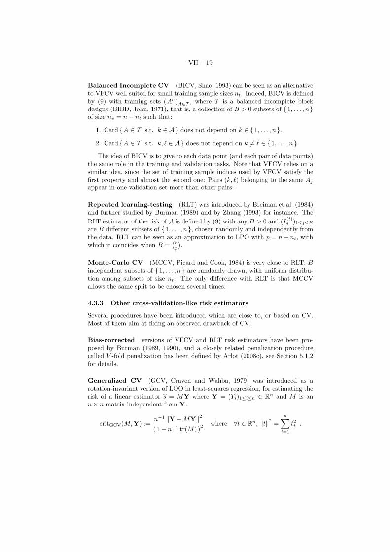
Generalized CV (GCV, Craven and Wahba, 1979) was introduced as arotation-invariant version of LOO in least-squares regression, for estimating therisk of a linear estimator s = MY where Y = (Yi)1≤i≤n ∈ Rn and M is ann× n matrix independent from Y:
critGCV(M,Y) :=n−1 ‖Y −MY‖2
(1− n−1 tr(M) )2where ∀t ∈ Rn, ‖t‖2 =
n∑i=1
t2i .
VII – 20
GCV is actually closer to CL (Mallows, 1973) than to CV, since GCV can beseen as an approximation to CL with a particular estimator of the variance(Efron, 1986). The efficiency of GCV has been proved in various frameworks,in particular by Li (1985, 1987) and by Cao and Golubev (2006).
Analytic Approximation When CV is used for selecting among linear mod-els, Shao (1993) proposed an analytic approximation to LPO with p ∼ n, whichis called APCV.
LOO bootstrap and .632 bootstrap The bootstrap is often used for stabi-lizing an estimator or an algorithm, replacing A(Dn) by the average of A(D?
n)over several bootstrap resamples D?
n. This idea was applied by Efron (1983)to the LOO estimator of the risk, leading to the LOO bootstrap. Noting thatthe LOO bootstrap was biased, Efron (1983) gave a heuristic argument leadingto the .632 bootstrap estimator of the risk, later modified into the .632+ boot-strap by Efron and Tibshirani (1997). The main drawback of these proceduresis the weakness of their theoretical justifications. Only empirical studies havesupported the good behaviour of .632+ bootstrap (Efron and Tibshirani, 1997;Molinaro et al., 2005).
4.4 Historical remarksSimple validation or hold-out was the first CV-like procedure. It was introducedin the psychology area (Larson, 1931) from the need for a reliable alternativeto the resubstitution error, as illustrated by Anderson et al. (1972). The hold-out was used by Herzberg (1969) for assessing the quality of predictors. Theproblem of choosing the training set was first considered by Stone (1974), where“controllable” and “uncontrollable” data splits were distinguished; an instanceof uncontrollable division can be found in the book by Simon (1971).
A primitive LOO procedure was used by Hills (1966) and by Lachenbruchand Mickey (1968) for evaluating the error rate of a prediction rule, and aprimitive formulation of LOO can be found in a paper by Mosteller and Tukey(1968). Nevertheless, LOO was actually introduced independently by Stone(1974), by Allen (1974) and by Geisser (1975). The relationship between LOOand the jackknife (Quenouille, 1949), which both rely on the idea of removing oneobservation from the sample, has been discussed by Stone (1974) for instance.
The hold-out and CV were originally used only for estimating the risk of analgorithm. The idea of using CV for model selection arose in the discussion ofa paper by Efron and Morris (1973) and in a paper by Geisser (1974). The firstauthor to study LOO as a model selection procedure was Stone (1974), whoproposed to use LOO again for estimating the risk of the selected model.
VII – 21
5 Statistical properties of cross-validation esti-mators of the risk
Understanding the behaviour of CV for model selection, which is the purposeof this survey, requires first to analyze the performances of CV as an estimatorof the risk of a single algorithm. Two main properties of CV estimators of therisk are of particular interest: their bias, and their variance.
5.1 BiasDealing with the bias incurred by CV estimates can be made by two strategies:evaluating the amount of bias in order to choose the least biased CV procedure,or correcting for this bias.
5.1.1 Theoretical assessment of the bias
The independence of the training and the validation samples imply that forevery algorithm A and any I(t) ⊂ {1, . . . , n} with cardinality nt,
E[LH−O
(A;Dn; I(t)
)]= E
[γ
(A
(D(t)
n
); ξ
)]= E [LP (A (Dnt ) ) ] .
Therefore, assuming that Card(I(t)j ) = nt for j = 1, . . . , B, the expectation of
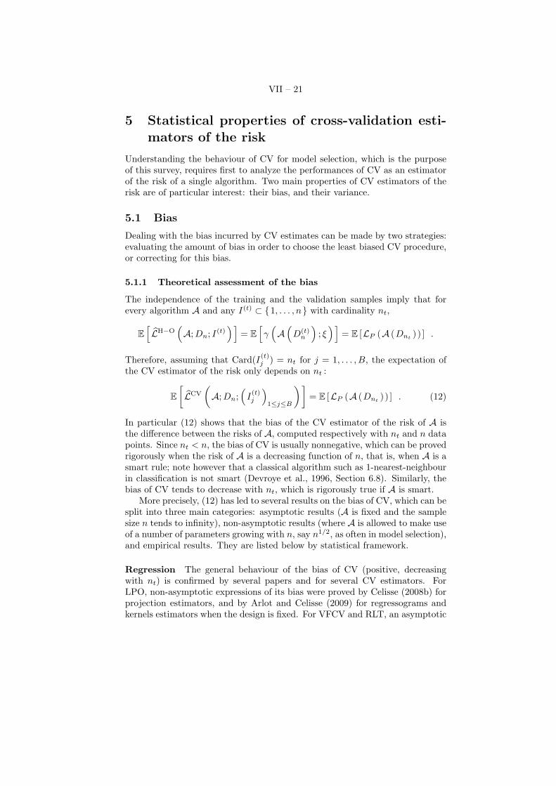
the CV estimator of the risk only depends on nt :
E[LCV
(A;Dn;
(I(t)j
)1≤j≤B
)]= E [LP (A (Dnt
) ) ] . (12)
In particular (12) shows that the bias of the CV estimator of the risk of A isthe difference between the risks of A, computed respectively with nt and n datapoints. Since nt < n, the bias of CV is usually nonnegative, which can be provedrigorously when the risk of A is a decreasing function of n, that is, when A is asmart rule; note however that a classical algorithm such as 1-nearest-neighbourin classification is not smart (Devroye et al., 1996, Section 6.8). Similarly, thebias of CV tends to decrease with nt, which is rigorously true if A is smart.
More precisely, (12) has led to several results on the bias of CV, which can besplit into three main categories: asymptotic results (A is fixed and the samplesize n tends to infinity), non-asymptotic results (where A is allowed to make useof a number of parameters growing with n, say n1/2, as often in model selection),and empirical results. They are listed below by statistical framework.
Regression The general behaviour of the bias of CV (positive, decreasingwith nt) is confirmed by several papers and for several CV estimators. ForLPO, non-asymptotic expressions of its bias were proved by Celisse (2008b) forprojection estimators, and by Arlot and Celisse (2009) for regressograms andkernels estimators when the design is fixed. For VFCV and RLT, an asymptotic
VII – 22
expansion of their bias was yielded by Burman (1989) for least-squares esti-mators in linear regression, and extended to spline smoothing (Burman, 1990).Note finally that Efron (1986) proved non-asymptotic analytic expressions ofthe expectations of the LOO and GCV estimators of the risk in regression withbinary data (see also Efron, 1983, for some explicit calculations).
Density estimation shows a similar picture. Non-asymptotic expressionsfor the bias of LPO estimators for kernel and projection estimators with thequadratic risk were proved by Celisse and Robin (2008) and by Celisse (2008a).Asymptotic expansions of the bias of the LOO estimator for histograms and ker-nel estimators were previously proved by Rudemo (1982); see Bowman (1984) forsimulations. Hall (1987) derived similar results with the log-likelihood contrastfor kernel estimators, and related the performance of LOO to the interactionbetween the kernel and the tails of the target density s.
Classification For the simple problem of discriminating between two popula-tions with shifted distributions, Davison and Hall (1992) compared the asymp-totical bias of LOO and bootstrap, showing the superiority of the LOO whenthe shift size is n−1/2 : As n tends to infinity, the bias of LOO stays of or-der n−1, whereas that of bootstrap worsens to the order n−1/2. On realisticsynthetic and real biological data, Molinaro et al. (2005) compared the bias ofLOO, VFCV and .632+ bootstrap: The bias decreases with nt, and is generallyminimal for LOO. Nevertheless, the 10-fold CV bias is nearly minimal uniformlyover their experiments. In the same experiments, .632+ bootstrap exhibits thesmallest bias for moderate sample sizes and small signal-to-noise ratios, but amuch larger bias otherwise.
CV-calibrated algorithms When a family of algorithm (Aλ )λ∈Λ is given,and λ is chosen by minimizing LCV(Aλ;Dn) over λ, LCV(Abλ;Dn) is biasedfor estimating the risk of Abλ(Dn), as reported from simulation experimentsby Stone (1974) for the LOO, and by Jonathan et al. (2000) for VFCV inthe variable selection setting. This bias is of different nature compared to theprevious frameworks. Indeed, LCV(Abλ, Dn) is biased simply because λ waschosen using the same data as LCV(Aλ, Dn). This phenomenon is similar to theoptimism of LPn
( s (Dn) ) as an estimator of the loss of s (Dn). The correctway of estimating the risk of Abλ(Dn) with CV is to consider the full algorithmA′ : Dn 7→ Abλ(Dn)(Dn), and then to compute LCV (A′;Dn ). The resultingprocedure is called “double cross” by Stone (1974).
5.1.2 Correction of the bias
An alternative to choosing the CV estimator with the smallest bias is to correctfor the bias of the CV estimator of the risk. Burman (1989, 1990) proposed a
VII – 23
corrected VFCV estimator, defined by
LcorrVF(A;Dn) = LVF ( s;Dn ) + LPn(A(Dn) )− 1
V
V∑j=1
LPn
(A(D(−Aj)
n ))
,
and a corrected RLT estimator was defined similarly. Both estimators havebeen proved to be asymptotically unbiased for least-squares estimators in linearregression.
When the Ajs have exactly the same size n/V , the corrected VFCV criterionis equal to the sum of the empirical risk and the V -fold penalty (Arlot, 2008c),defined by
penVF(A;Dn) =V − 1
V
V∑j=1
[LPn
(A(D(−Aj)
n ))− L
P(−Aj)n
(A(D(−Aj)
n ))]
.
The V -fold penalized criterion was proved to be (almost) unbiased in the non-asymptotic framework for regressogram estimators.
5.2 VarianceCV estimators of the risk using training sets of the same size nt havethe same bias, but they still behave quite differently; their variancevar(LCV(A;Dn; (I(t)
j )1≤j≤B)) captures most of the information to explain thesedifferences.
5.2.1 Variability factors
Assume that Card(I(t)j ) = nt for every j. The variance of CV results from the
combination of several factors, in particular (nt, nv) and B.
Influence of (nt, nv) Let us consider the hold-out estimator of the risk. Fol-lowing in particular Nadeau and Bengio (2003),
var[LH−O
(A;Dn; I(t)
)]= E
[var
(L
P(v)n
(A(D(t)
n )) ∣∣∣ D(t)
n
)]+ var [LP (A(Dnt) ) ]
=1nv
E[var
(γ ( s , ξ ) | s = A(D(t)
n ))]
+ var [LP (A(Dnt) ) ] . (13)
The first term, proportional to 1/nv, shows that more data for validationdecreases the variance of LH−O, because it yields a better estimator ofLP
(A(D(t)
n ))
. The second term shows that the variance of LH−O also depends
on the distribution of LP
(A(D(t)
n ))
around its expectation; in particular, itstrongly depends on the stability of A.
VII – 24
Stability and variance When A is unstable, LLOO (A ) has often beenpointed out as a variable estimator (Section 7.10, Hastie et al., 2001; Breiman,1996). Conversely, this trend disappears when A is stable, as noticed by Moli-naro et al. (2005) from a simulation experiment.
The relation between the stability of A and the variance of LCV (A ) waspointed out by Devroye and Wagner (1979) in classification, through upperbounds on the variance of LLOO (A ). Bousquet and Elisseff (2002) extendedthese results to the regression setting, and proved upper bounds on the maximalupward deviation of LLOO (A ).
Note finally that several approaches based on the bootstrap have been pro-posed for reducing the variance of LLOO (A ), such as LOO bootstrap, .632bootstrap and .632+ bootstrap (Efron, 1983); see also Section 4.3.3.
Partial splitting and variance When (nt, nv) is fixed, the variability ofCV tends to be larger for partial data splitting methods than for LPO. Indeed,having to choose B <
(nnt
)subsets (I(t)
j )1≤j≤B of {1, . . . , n}, usually randomly,induces an additional variability compared to LLPO with p = n − nt. In thecase of MCCV, this variability decreases like B−1 since the I
(t)j are chosen
independently. The dependence on B is slightly different for other CV estimatorssuch as RLT or VFCV, because the I
(t)j are not independent. In particular, it
is maximal for the hold-out, and minimal (null) for LOO (if nt = n − 1) andLPO (with p = n− nt).
Note that the dependence on V for VFCV is more complex to evaluate, sinceB, nt, and nv simultaneously vary with V . Nevertheless, a non-asymptotic the-oretical quantification of this additional variability of VFCV has been obtainedby Celisse and Robin (2008) in the density estimation framework (see also em-pirical considerations by Jonathan et al., 2000).
5.2.2 Theoretical assessment of the variance
Understanding precisely how var(LCV(A)) depends on the splitting scheme iscomplex in general, since nt and nv have a fixed sum n, and the number of splitsB is generally linked with nt (for instance, for LPO and VFCV). Furthermore,the variance of CV behaves quite differently in different frameworks, dependingin particular on the stability of A. The consequence is that contradictory resultshave been obtained in different frameworks, in particular on the value of Vfor which the VFCV estimator of the risk has a minimal variance (Burman,1989; Hastie et al., 2001, Section 7.10). Despite the difficulty of the problem,the variance of several CV estimators of the risk has been assessed in severalframeworks, as detailed below.
Regression In the linear regression setting, Burman (1989) yielded asymp-totic expansions of the variance of the VFCV and RLT estimators of the riskwith homoscedastic data. The variance of RLT decreases with B, and in the
VII – 25
case of VFCV, in a particular setting,
var(LVF(A)
)=
2σ2
n+
4σ4
n2
[4 +
4V − 1
+2
(V − 1)2+
1(V − 1)3
]+ o
(n−2
).
The asymptotical variance of the VFCV estimator of the risk decreases with V ,implying that LOO asymptotically has the minimal variance.
Non-asymptotic closed-form formulas of the variance of the LPO estimatorof the risk have been proved by Celisse (2008b) in regression, for projection andkernel estimators for instance. On the variance of RLT in the regression setting,see the asymptotic results of Girard (1998) for Nadaraya-Watson kernel estima-tors, as well as the non-asymptotic computations and simulation experimentsby Nadeau and Bengio (2003) with several learning algorithms.
Density estimation Non-asymptotic closed-form formulas of the variance ofthe LPO estimator of the risk have been proved by Celisse and Robin (2008)and by Celisse (2008a) for projection and kernel estimators. In particular, thedependence of the variance of LLPO on p has been quantified explicitly forhistogram and kernel estimators by Celisse and Robin (2008).
Classification For the simple problem of discriminating between two popu-lations with shifted distributions, Davison and Hall (1992) showed that the gapbetween asymptotic variances of LOO and bootstrap becomes larger when dataare noisier. Nadeau and Bengio (2003) made non-asymptotic computations andsimulation experiments with several learning algorithms. Hastie et al. (2001)empirically showed that VFCV has a minimal variance for some 2 < V < n,whereas LOO usually has a large variance; this fact certainly depends on thestability of the algorithm considered, as showed by simulation experiments byMolinaro et al. (2005).
5.2.3 Estimation of the variance
There is no universal—valid under all distributions—unbiased estimator of thevariance of RLT (Nadeau and Bengio, 2003) and VFCV estimators (Bengio andGrandvalet, 2004). In particular, Bengio and Grandvalet (2004) recommend theuse of variance estimators taking into account the correlation structure betweentest errors; otherwise, the variance of CV can be strongly underestimated.
Despite these negative results, (biased) estimators of the variance of LCV
have been proposed by Nadeau and Bengio (2003), by Bengio and Grandvalet(2004) and by Markatou et al. (2005), and tested in simulation experiments inregression and classification. Furthermore, in the framework of density estima-tion with histograms, Celisse and Robin (2008) proposed an estimator of thevariance of the LPO risk estimator. Its accuracy is assessed by a concentrationinequality. These results have recently been extended to projection estimatorsby Celisse (2008a).
VII – 26
6 Cross-validation for efficient model selectionThis section tackles the properties of CV procedures for model selection whenthe goal is estimation (see Section 2.2).
6.1 Relationship between risk estimation and model se-lection
As shown in Section 3.1, minimizing an unbiased estimator of the risk leads to anefficient model selection procedure. One could conclude here that the best CVprocedure for estimation is the one with the smallest bias and variance (at leastasymptotically), for instance, LOO in the least-squares regression framework(Burman, 1989).
Nevertheless, the best CV estimator of the risk is not necessarily the bestmodel selection procedure. For instance, Breiman and Spector (1992) observedthat uniformly over the models, the best risk estimator is LOO, whereas 10-fold CV is more accurate for model selection. Three main reasons for such adifference can be invoked. First, the asymptotic framework (A fixed, n → ∞)may not apply to models close to the oracle, which typically has a dimensiongrowing with n when s does not belong to any model. Second, as explained inSection 3.2, estimating the risk of each model with some bias can be beneficialand compensate the effect of a large variance, in particular when the signal-to-noise ratio is small. Third, for model selection, what matters is not that everyestimate of the risk has small bias and variance, but more that
sign (crit(m1)− crit(m2) ) = sign (LP ( sm1 )− LP ( sm2 ) )
with the largest probability for models m1,m2 near the oracle.Therefore, specific studies are required to evaluate the performances of the
various CV procedures in terms of model selection efficiency. In most frame-works, the model selection performance directly follows from the properties ofCV as an estimator of the risk, but not always.
6.2 The global pictureLet us start with the classification of model selection procedures made by Shao(1997) in the linear regression framework, since it gives a good idea of theperformance of CV procedures for model selection in general. Typically, theefficiency of CV only depends on the asymptotics of nt/n :
• When nt ∼ n, CV is asymptotically equivalent to Mallows’ Cp, henceasymptotically optimal.
• When nt ∼ λn with λ ∈ (0, 1), CV is asymptotically equivalent to GICκ
with κ = 1+λ−1, which is defined as AIC with a penalty multiplied by κ/2.Hence, such CV procedures are overpenalizing by a factor (1+λ)/(2λ) > 1.
VII – 27
The above results have been proved by Shao (1997) for LPO (see also Li, 1987,for the LOO); they also hold for RLT when B � n2 since RLT is then equivalentto LPO (Zhang, 1993).
In a general statistical framework, the model selection performance ofMCCV, VFCV, LOO, LOO Bootstrap, and .632 bootstrap for selection amongminimum contrast estimators was studied in a series of papers (van der Laan andDudoit, 2003; van der Laan et al., 2004, 2006; van der Vaart et al., 2006); theseresults apply in particular to least-squares regression and density estimation.It turns out that under mild conditions, an oracle-type inequality is proved,showing that up to a multiplying factor Cn → 1, the risk of CV is smaller thanthe minimum of the risks of the models with a sample size nt. In particular,in most frameworks, this implies the asymptotic optimality of CV as soon asnt ∼ n. When nt ∼ λn with λ ∈ (0, 1), this naturally generalizes Shao’s results.
6.3 Results in various frameworksThis section gathers results about model selection performances of CV whenthe goal is estimation, in various frameworks. Note that model selection is con-sidered here with a general meaning, including in particular bandwidth choicefor kernel estimators.
Regression First, the results of Section 6.2 suggest that CV is suboptimalwhen nt is not asymptotically equivalent to n. This fact has been proved rigor-ously for VFCV when V = O(1) with regressograms (Arlot, 2008c): with largeprobability, the risk of the model selected by VFCV is larger than 1 + κ(V )times the risk of the oracle, with κ(V ) > 0 for every fixed V . Note howeverthat the best V for VFCV is not the largest one in every regression framework,as shown empirically in linear regression (Breiman and Spector, 1992; Herzbergand Tsukanov, 1986); Breiman (1996) proposed to explain this phenomenonby relating the stability of the candidate algorithms and the model selectionperformance of LOO in various regression frameworks.
Second, the “universality” of CV has been confirmed by showing that it natu-rally adapts to heteroscedasticity of data when selecting among regressograms.Despite its suboptimality, VFCV with V = O(1) satisfies a non-asymptoticoracle inequality with constant C > 1 (Arlot, 2008c). Furthermore, V -foldpenalization (which often coincides with corrected VFCV, see Section 5.1.2)satisfies a non-asymptotic oracle inequality with Cn → 1 as n → +∞, bothwhen V = O(1) (Arlot, 2008c) and when V = n (Arlot, 2008a). Note thatn-fold penalization is very close to LOO, suggesting that it is also asymptoti-cally optimal with heteroscedastic data. Simulation experiments in the contextof change-point detection confirmed that CV adapts well to heteroscedasticity,contrary to usual model selection procedures in the same framework (Arlot andCelisse, 2009).
The performances of CV have also been assessed for other kinds of estimatorsin regression. For choosing the number of knots in spline smoothing, Burman(1990) proved that corrected versions of VFCV and RLT are asymptotically
VII – 28
optimal provided n/(Bnv) = O(1). Furthermore, in kernel regression, severalCV methods have been compared to GCV in kernel regression by Härdle et al.(1988) and by Girard (1998); the conclusion is that GCV and related criteriaare computationally more efficient than MCCV or RLT, for a similar statisticalperformance.
Finally, note that asymptotic results about CV in regression have beenproved by Györfi et al. (2002), and an oracle inequality with constant C > 1 hasbeen proved by Wegkamp (2003) for the hold-out, with least-squares estimators.
Density estimation CV performs similarly than in regression for selectingamong least-squares estimators (van der Laan et al., 2004): It yields a risksmaller than the minimum of the risk with a sample size nt. In particular, non-asymptotic oracle inequalities with constant C > 1 have been proved by Celisse(2008b) for the LPO when p/n ∈ [a, b], for some 0 < a < b < 1.
The performance of CV for selecting the bandwidth of kernel density esti-mators has been studied in several papers. With the least-squares contrast, theefficiency of LOO was proved by Hall (1983) and generalized to the multivari-ate framework by Stone (1984); an oracle inequality asymptotically leading toefficiency was recently proved by Dalelane (2005). With the Kullback-Leiblerdivergence, CV can suffer from troubles in performing model selection (see alsoSchuster and Gregory, 1981; Chow et al., 1987). The influence of the tails ofthe target s was studied by Hall (1987), who gave conditions under which CVis efficient and the chosen bandwidth is optimal at first-order.
Classification In the framework of binary classification by intervals (that is,with X = [0, 1] and piecewise constant classifiers), Kearns et al. (1997) provedan oracle inequality for the hold-out. Furthermore, empirical experiments showthat CV yields (almost) always the best performance, compared to deterministicpenalties (Kearns et al., 1997). On the contrary, simulation experiments byBartlett et al. (2002) in the same setting showed that random penalties such asRademacher complexity and maximal discrepancy usually perform much betterthan hold-out, which is shown to be more variable.
Nevertheless, the hold-out still enjoys quite good theoretical properties: Itwas proved to adapt to the margin condition by Blanchard and Massart (2006),a property nearly unachievable with usual model selection procedures (see alsoMassart, 2007, Section 8.5). This suggests that CV procedures are naturallyadaptive to several unknown properties of data in the statistical learning frame-work.
The performance of the LOO in binary classification was related to thestability of the candidate algorithms by Kearns and Ron (1999); they provedoracle-type inequalities called “sanity-check bounds”, describing the worst-caseperformance of LOO (see also Bousquet and Elisseff, 2002).
An experimental comparison of several CV methods and bootstrap-basedCV (in particular .632+ bootstrap) in classification can also be found in papersby Efron (1986) and Efron and Tibshirani (1997).
VII – 29
7 Cross-validation for identificationLet us now focus on model selection when the goal is to identify the “true model”Sm0 , as described in Section 2.3. In this framework, asymptotic optimality isreplaced by (model) consistency, that is,
P (m(Dn) = m0 ) −−−−→n→∞
1 .
Classical model selection procedures built for identification, such as BIC, aredescribed in Section 3.3.
7.1 General conditions towards model consistencyAt first sight, it may seem strange to use CV for identification: LOO, whichis the pioneering CV procedure, is actually closely related to the unbiased riskestimation principle, which is only efficient when the goal is estimation. Fur-thermore, estimation and identification are somehow contradictory goals, asexplained in Section 2.4.
This intuition about inconsistency of some CV procedures is confirmed byseveral theoretical results. Shao (1993) proved that several CV methods areinconsistent for variable selection in linear regression: LOO, LPO, and BICVwhen lim infn→∞(nt/n) > 0. Even if these CV methods asymptotically selectall the true variables with probability 1, the probability that they select toomuch variables does not tend to zero. More generally, Shao (1997) proved thatCV procedures behave asymptotically like GICλn with λn = 1 + n/nt, whichleads to inconsistency as soon as n/nt = O(1).
In the context of ordered variable selection in linear regression, Zhang (1993)computed the asymptotic value of the probability of selecting the true modelfor several CV procedures. He also numerically compared the values of thisprobability for the same CV procedures in a specific example. For LPO withp/n → λ ∈ (0, 1) as n tends to +∞, P (m = m0 ) increases with λ. The result isslightly different for VFCV: P (m = m0 ) increases with V (hence, it is maximalfor the LOO, which is the worst case of LPO). The variability induced by thenumber V of splits seems to be more important here than the bias of VFCV.Nevertheless, P (m = m0 ) is almost constant between V = 10 and V = n, sothat taking V > 10 is not advised for computational reasons.
These results suggest that if the training sample size nt is negligible in frontof n, then model consistency could be obtained. This has been confirmed theo-retically by Shao (1993, 1997) for the variable selection problem in linear regres-sion: CV is consistent when n � nt →∞, in particular RLT, BICV (defined inSection 4.3.2) and LPO with p = pn ∼ n and n− pn →∞.
Therefore, when the goal is to identify the true model, a larger proportion ofthe data should be put in the validation set in order to improve the performance.This phenomenon is somewhat related to the cross-validation paradox (Yang,2006).
VII – 30
7.2 Refined analysis for the algorithm selection problemThe behaviour of CV for identification is better understood by considering amore general framework, where the goal is to select among statistical algorithmsthe one with the fastest convergence rate. Yang (2006, 2007) considered thisproblem for two candidate algorithms (or more generally any finite number ofalgorithms). Let us mention here that Stone (1977) considered a few specificexamples of this problem, and showed that LOO can be inconsistent for choosingthe best among two “good” estimators.
The conclusion of Yang’s papers is that the sufficient condition on nt forthe consistency in selection of CV strongly depends on the convergence rates(rn,i )i=1,2 of the candidate algorithms. Let us assume that rn,1 and rn,2 differat least by a multiplicative constant C > 1. Then, in the regression framework,if the risk of si is measured by E ‖si − s‖2, Yang (2007) proved that the hold-out, VFCV, RLT and LPO with voting (CV-v, see Section 4.2.2) are consistentin selection if
nv, nt →∞ and√
nv maxi
rnt,i →∞ , (14)
under some conditions on ‖si − s‖p for p = 2, 4,∞. In the classification frame-work, if the risk of si is measured by P ( si 6= s ), Yang (2006) proved the sameconsistency result for CV-v under the condition
nv, nt →∞ andnv maxi r2
nt,i
snt
→∞ , (15)
where sn is the convergence rate of P ( s1(Dn) 6= s2(Dn) ).Intuitively, consistency holds as soon as the uncertainty of each estimate of
the risk (roughly proportional to n−1/2v ) is negligible in front of the risk gap
|rnt,1 − rnt,2| (which is of the same order as maxi rnt,i). This condition holdseither when at least one of the algorithms converges at a non-parametric rate,or when nt � n, which artificially widens the risk gap.
Empirical results in the same direction were proved by Dietterich (1998)and by Alpaydin (1999), leading to the advice that V = 2 is the best choicewhen VFCV is used for comparing two learning procedures. See also the re-sults by Nadeau and Bengio (2003) about CV considered as a testing procedurecomparing two candidate algorithms.
The sufficient conditions (14) and (15) can be simplified depending onmaxi rn,i, so that the ability of CV to distinguish between two algorithms de-pends on their convergence rates. On the one hand, if maxi rn,i ∝ n−1/2, then(14) or (15) only hold when nv � nt → ∞ (under some conditions on sn inclassification). Therefore, the cross-validation paradox holds for comparing al-gorithms converging at the parametric rate (model selection when a true modelexists being only a particular case). Note that possibly stronger conditions canbe required in classification where algorithms can converge at fast rates, betweenn−1 and n−1/2.
On the other hand, (14) and (15) are milder conditions when maxi rn,i �n−1/2: They are implied by nt/nv = O(1), and they even allow nt ∼ n (under
VII – 31
some conditions on sn in classification). Therefore, non-parametric algorithmscan be compared by more usual CV procedures (nt > n/2), even if LOO is stillexcluded by conditions (14) and (15).
Note that according to a simulation experiments, CV with averaging (thatis, CV as usual) and CV with voting are equivalent at first but not at secondorder, so that they can differ when n is small (Yang, 2007).
8 Specificities of some frameworksOriginally, the CV principle has been proposed for i.i.d. observations and usualcontrasts such as least-squares and log-likelihood. Therefore, CV proceduresmay have to be modified in other specific frameworks, such as estimation inpresence of outliers or with dependent data.
8.1 Density estimationIn the density estimation framework, some specific modifications of CV havebeen proposed.
First, Hall et al. (1992) defined the “smoothed CV”, which consists in pre-smoothing the data before using CV, an idea related to the smoothed bootstrap.They proved that smoothed CV yields an excellent asymptotical model selectionperformance under various smoothness conditions on the density.
Second, when the goal is to estimate the density at one point (and notglobally), Hall and Schucany (1989) proposed a local version of CV and provedits asymptotic optimality.
8.2 Robustness to outliersIn presence of outliers in regression, Leung (2005) studied how CV must bemodified to get both asymptotic efficiency and a consistent bandwidth estimator(see also Leung et al., 1993).
Two changes are possible to achieve robustness: Choosing a “robust” regres-sor, or choosing a robust loss-function. In presence of outliers, classical CV witha non-robust loss function has been shown to fail by Härdle (1984).
Leung (2005) described a CV procedure based on robust losses like L1 andHuber’s (Huber, 1964) ones. The same strategy remains applicable to othersetups like linear models in Ronchetti et al. (1997).
8.3 Time series and dependent observationsAs explained in Section 4.1, CV is built upon the heuristics that part of thesample (the validation set) can play the role of new data with respect to therest of the sample (the training set). “New” means that the validation set isindependent from the training set with the same distribution. Therefore, whendata ξ1, . . . , ξn are not independent, CV must be modified, like other model
VII – 32
selection procedures (in non-parametric regression with dependent data, see thereview by Opsomer et al., 2001).
Let us first consider the statistical framework of Section 1 with ξ1, . . . , ξn
identically distributed but not independent. Then, when for instance data arepositively correlated, Hart and Wehrly (1986) proved that CV overfits for choos-ing the bandwidth of a kernel estimator in regression (see also Chu and Marron,1991; Opsomer et al., 2001).
The main approach used in the literature for solving this issue is to chooseI(t) and I(v) such that mini∈I(t), j∈I(v) |i− j| > h > 0, where h controls the dis-tance from which observations i and j are independent. For instance, the LOOcan be changed into: I(v) = {J } where J is uniformly chosen in {1, . . . , n},and I(t) = {1, . . . , J − h− 1, J + h + 1, . . . , n}, a method called “modified CV”by Chu and Marron (1991) in the context of bandwidth selection. Then, forshort range dependences, ξi is almost independent from ξj when |i− j| > h islarge enough, so that (ξj )j∈I(t) is almost independent from (ξj )j∈I(v) . Severalasymptotic optimality results have been proved on modified CV, for instanceby Hart and Vieu (1990) for bandwidth choice in kernel density estimation,when data are α-mixing (hence, with a short range dependence structure) andh = hn → ∞ “not too fast”. Note that modified CV also enjoys some asymp-totic optimality results with long-range dependences, as proved by Hall et al.(1995), even if an alternative block bootstrap method seems more appropriatein such a framework.
Several alternatives to modified CV have also been proposed. The “h-blockCV” (Burman et al., 1994) is modified CV plus a corrective term, similarly to thebias-corrected CV by Burman (1989) (see Section 5.1). Simulation experimentsin several (short range) dependent frameworks show that this corrective termmatters when h/n is not small, in particular when n is small.
The “partitioned CV” has been proposed by Chu and Marron (1991) forbandwidth selection: An integer g > 0 is chosen, a bandwidth λk is chosen byCV based upon the subsample (ξk+gj )j≥0 for each k = 1, . . . , g, and the selectedbandwidth is a combination of (λk).
When a parametric model is available for the dependency structure, Hart(1994) proposed the “time series CV”.
An important framework where data often are dependent is time-series anal-ysis, in particular when the goal is to predict the next observation ξn+1 from thepast ξ1, . . . , ξn. When data are stationary, h-block CV and similar approachescan be used to deal with (short range) dependences. Nevertheless, Burman andNolan (1992) proved in some specific framework that unaltered CV is asymptoticoptimal when ξ1, . . . , ξn is a stationary Markov process.
On the contrary, using CV for non-stationary time-series is a quite difficultproblem. The only reasonable approach in general is the hold-out, that is,I(t) = {1, . . . ,m} and I(v) = {m + 1, . . . , n} for some deterministic m. Eachmodel is first trained with (ξj )j∈I(t) . Then, it is used for predicting successively
VII – 33
ξm+1 from (ξj )j≤m, ξm+2 from (ξj )j≤m+1, and so on. The model with thesmallest average error for predicting (ξj )j∈I(v) from the past is chosen.
8.4 Large number of modelsAs mentioned in Section 3, model selection procedures estimating unbiasedlythe risk of each model fail when, in particular, the number of models growsexponentially with n (Birgé and Massart, 2007). Therefore, CV cannot be useddirectly, except maybe with nt � n, provided nt is well chosen (see Section 6and Celisse, 2008b, Chapter 6).
For least-squares regression with homoscedastic data, Wegkamp (2003) pro-posed to add to the hold-out estimator of the risk a penalty term dependingon the number of models. This method is proved to satisfy a non-asymptoticoracle inequality with leading constant C > 1.
Another general approach was proposed by Arlot and Celisse (2009) in thecontext of multiple change-point detection. The idea is to perform model se-lection in two steps: First, gather the models (Sm )m∈Mn
into meta-models(SD)D∈Dn
, where Dn denotes a set of indices such that Card(Dn) grows atmost polynomially with n. Inside each meta-model SD =
⋃m∈Mn(D) Sm, sD is
chosen from data by optimizing a given criterion, for instance the empirical con-trast LPn ( t ), but other criteria can be used. Second, CV is used for choosingamong ( sD )D∈Dn
. Simulation experiments show this simple trick automaticallytakes into account the cardinality of Mn, even when data are heteroscedastic,contrary to other model selection procedures built for exponential collection ofmodels which all assume homoscedasticity of data.
9 Closed-form formulas and fast computationResampling strategies, like CV, are known to be time consuming. The naive im-plementation of CV has a computational complexity of B times the complexityof training each algorithm A, which is usually intractable for LPO, even withp = 1. The computational cost of VFCV or RLT can still be quite costly whenB > 10 in many practical problems. Nevertheless, closed-form formulas forCV estimators of the risk can be obtained in several frameworks, which greatlydecreases the computational cost of CV.
In density estimation, closed-form formulas have been originally derived byRudemo (1982) and by Bowman (1984) for the LOO risk estimator of histogramsand kernel estimators. These results have been recently extended by Celisseand Robin (2008) to the LPO risk estimator with the quadratic loss. Similarresults are more generally available for projection estimators as settled by Celisse(2008a). Intuitively, such formulas can be obtained provided the number N ofvalues taken by the B =
(nnv
)hold-out estimators of the risk, corresponding to
different data splittings, is at most polynomial in the sample size.

VII – 34
For least-squares estimators in linear regression, Zhang (1993) proved aclosed-form formula for the LOO estimator of the risk. Similar results havebeen obtained by Wahba (1975, 1977), and by Craven and Wahba (1979) in thespline smoothing context as well. These papers led in particular to the definitionof GCV (see Section 4.3.3) and related procedures, which are often used insteadof CV (with a naive implementation) because of their small computational cost,as emphasized by Girard (1998).
Closed-form formulas for the LPO estimator of the risk were also obtained byCelisse (2008b) in regression for kernel and projection estimators, in particularfor regressograms. An important property of these closed-form formulas is theiradditivity: For a regressogram associated to a partition (Iλ)λ∈Λm of X , theLPO estimator of the risk can be written as a sum over λ ∈ Λm of termswhich only depend on observations (Xi, Yi) such that Xi ∈ Iλ. Therefore,dynamic programming (Bellman and Dreyfus, 1962) can be used for minimizingthe LPO estimator of the risk over the set of partitions of X in D pieces. Asan illustration, Arlot and Celisse (2009) successfully applied this strategy inthe change-point detection framework. Note that the same idea can be usedwith VFCV or RLT, but for a larger computational cost since no closed-formformulas are available for these CV methods.
Finally, in frameworks where no closed-form formula can be proved, someefficient algorithms exist for avoiding to recompute LH−O(A;Dn; I(t)
j ) fromscratch for each data splitting I
(t)j . These algorithms rely on updating formulas
such as the ones by Ripley (1996) for LOO in linear and quadratic discriminantanalysis; this approach makes LOO as expensive to compute as the empiricalrisk.
Very similar formulas are also available for LOO and the k-nearest neigh-bours estimator in classification (Daudin and Mary-Huard, 2008).
10 Conclusion: which cross-validation methodfor which problem?
This conclusion collects a few guidelines aiming at helping CV users, first in-terpreting the results of CV, second appropriately using CV in each specificproblem.
10.1 The general pictureDrawing a general conclusion on CV methods is an impossible task because ofthe variety of frameworks where CV can be used, which induces a variety ofbehaviors of CV. Nevertheless, we can still point out the three main criteria totake into account for choosing a CV method for a particular model selectionproblem:
• Bias: CV roughly estimates the risk of a model with a sample size nt < n(see Section 5.1). Usually, this implies that CV overestimates the variance
VII – 35
term compared to the bias term in the bias-variance decomposition (2)with sample size n.When the goal is estimation and the signal-to-noise ratio (SNR) is large,the smaller bias usually is the better, which is obtained by taking nt ∼ n.Otherwise, CV can be asymptotically suboptimal. Nevertheless, when thegoal is estimation and the SNR is small, keeping a small upward bias forthe variance term often improves the performance, which is obtained bytaking nt ∼ κn with κ ∈ (0, 1). See Section 6.When the goal is identification, a large bias is often needed, which isobtained by taking nt � n; depending on the framework, larger values ofnt can also lead to model consistency, see Section 7.
• Variability: The variance of the CV estimator of the risk is usually adecreasing function of the number B of splits, for a fixed training size.When the number of splits is fixed, the variability of CV also dependson the training sample size nt. Usually, CV is more variable when nt iscloser to n. However, when B is linked with nt (as for VFCV or LPO),the variability of CV must be quantified precisely, which has been done infew frameworks. The only general conclusion on this point is that the CVmethod with minimal variability seems strongly framework-dependent, seeSection 5.2 for details.
• Computational complexity: Unless closed-form formulas or analytic ap-proximations are available (see Section 9), the complexity of CV is roughlyproportional to the number of data splits: 1 for the hold-out, V for VFCV,B for RLT or MCCV, n for LOO, and
(np
)for LPO.
The optimal trade-off between these three factors can be different for each prob-lem, depending for instance on the computational complexity of each estimator,on specificities of the framework considered, and on the final user’s trade-offbetween statistical performance and computational cost. Therefore, no “opti-mal CV method” can be pointed out before having taken into account the finaluser’s preferences.
Nevertheless, in density estimation, closed-form expressions of the LPO es-timator have been derived by Celisse and Robin (2008) with histograms andkernel estimators, and by Celisse (2008a) for projection estimators. These ex-pressions allow to perform LPO without additional computational cost, whichreduces the aforementioned trade-off to the easier bias-variability trade-off. Inparticular, Celisse and Robin (2008) proposed to choose p for LPO by minimiz-ing a criterion defined as the sum of a squared bias and a variance terms (seealso Politis et al., 1999, Chapter 9).
10.2 How the splits should be chosen?For hold-out, VFCV, and RLT, an important question is to choose a particularsequence of data splits.
VII – 36
First, should this step be random and independent from Dn, or take intoaccount some features of the problem or of the data? It is often recommendedto take into account the structure of data when choosing the splits. If dataare stratified, the proportions of the different strata should (approximately) bethe same in the sample and in each training and validation sample. Besides,the training samples should be chosen so that sm(D(t)
n ) is well defined for ev-ery training set; in the regressogram case, this led Arlot (2008c) and Arlot andCelisse (2009) to choose carefully the splitting scheme. In supervised classifica-tion, practitioners usually choose the splits so that the proportion of each classis the same in every validation sample as in the sample. Nevertheless, Breimanand Spector (1992) made simulation experiments in regression for comparingseveral splitting strategies. No significant improvement was reported from tak-ing into account the stratification of data for choosing the splits.
Another question related to the choice of (I(t)j )1≤j≤B is whether the I
(t)j
should be independent (like MCCV), slighly dependent (like RLT), or stronglydependent (like VFCV). It seems intuitive that giving similar roles to all datapoints in the B “training and validation tasks” should yield more reliable resultsas other methods. This intuition may explain why VFCV is much more usedthan RLT or MCCV. Similarly, Shao (1993) proposed a CV method called BICV,where every point and pair of points appear in the same number of splits, seeSection 4.3.2. Nevertheless, most recent theoretical results on the various CVprocedures are not accurate enough to distinguish which one may be the bestsplitting strategy: This remains a widely open theoretical question.
Note finally that the additional variability due to the choice of a sequence ofdata splits was quantified empirically by Jonathan et al. (2000) and theoreticallyby Celisse and Robin (2008) for VFCV.
10.3 V-fold cross-validationVFCV is certainly the most popular CV procedure, in particular because ofits mild computational cost. Nevertheless, the question of choosing V remainswidely open, even if indications can be given towards an appropriate choice.
A specific feature of VFCV—as well as exhaustive strategies—is that choos-ing V uniquely determines the size of the training set nt = n(V − 1)/V andthe number of splits B = V , hence the computational cost. Contradictoryphenomena then occur.
On the one hand, the bias of VFCV decreases with V since nt = n(1− 1/V )observations are used in the training set. On the other hand, the variance ofVFCV decreases with V for small values of V , whereas the LOO (V = n) isknown to suffer from a high variance in several frameworks such as classificationor density estimation. Note however that the variance of VFCV is minimal forV = n in some frameworks like linear regression (see Section 5.2). Furthermore,estimating the variance of VFCV from data is a difficult problem in general, seeSection 5.2.3.
When the goal of model selection is estimation, it is often reported in the
VII – 37
literature that the optimal V is between 5 and 10, because the statistical perfor-mance does not increase much for larger values of V , and averaging over 5 or 10splits remains computationally feasible (Hastie et al., 2001, Section 7.10). Evenif this claim is clearly true for many problems, the conclusion of this survey isthat better statistical performance can sometimes be obtained with other valuesof V , for instance depending on the SNR value.
When the SNR is large, the asymptotic comparison of CV procedures re-called in Section 6.2 can be trusted: LOO performs (nearly) unbiased risk es-timation hence is asymptotically optimal, whereas VFCV with V = O(1) issuboptimal. On the contrary, when the SNR is small, overpenalization canimprove the performance. Therefore, VFCV with V < n can yield a smallerrisk than LOO thanks to its bias and despite its variance when V is small (seesimulation experiments by Arlot, 2008c). Furthermore, other CV procedureslike RLT can be interesting alternatives to VFCV, since they allow to choosethe bias (through nt) independently from B, which mainly governs the variance.Another possible alternative is V -fold penalization, which is related to correctedVFCV (see Section 4.3.3).
When the goal of model selection is identification, the main drawback ofVFCV is that nt � n is often required for choosing consistently the true model(see Section 7), whereas VFCV does not allow nt < n/2. Depending on theframeworks, different (empirical) recommandations for choosing V can be foundin the literature. In ordered variable selection, the largest V seems to be thebetter, V = 10 providing results close to the optimal ones (Zhang, 1993). On thecontrary, Dietterich (1998) and Alpaydin (1999) recommend V = 2 for choosingthe best learning procedures among two candidates.
10.4 Future researchPerhaps the most important direction for future research would be to provide,in each specific framework, precise quantitative measures of the variance of CVestimators of the risk, depending on nt, the number of splits, and how thesplits are chosen. Up to now, only a few precise results have been obtainedin this direction, for some specific CV methods in linear regression or densityestimation (see Section 5.2). Proving similar results in other frameworks andfor more general CV methods would greatly help to choose a CV method forany given model selection problem.
More generally, most theoretical results are not precise enough to make anydistinction between the hold-out and CV methods having the same trainingsample size nt, because they are equivalent at first order. Second order termsdo matter for realistic values of n, which shows the dramatic need for theorythat takes into account the variance of CV when comparing CV methods suchas VFCV and RLT with nt = n(V − 1)/V but B 6= V .
VII – 38
ReferencesAkaike, H. (1970). Statistical predictor identification. Ann. Inst. Statist. Math.,
22:203–217.
Akaike, H. (1973). Information theory and an extension of the maximum like-lihood principle. In Second International Symposium on Information Theory(Tsahkadsor, 1971), pages 267–281. Akadémiai Kiadó, Budapest.
Allen, D. M. (1974). The relationship between variable selection and data aug-mentation and a method for prediction. Technometrics, 16:125–127.
Alpaydin, E. (1999). Combined 5 x 2 cv F test for comparing supervised clas-sification learning algorithms. Neur. Comp., 11(8):1885–1892.
Anderson, R. L., Allen, D. M., and B., C. F. (1972). Selectioon of predictorvariables in linear multiple regression. In bancroft, T. A., editor, In Statisticalpapers in Honor of George W. Snedecor. Iowa: iowa State University Press.
Arlot, S. (2007). Resampling and Model Selection. PhD thesis, University Paris-Sud 11. oai:tel.archives-ouvertes.fr:tel-00198803_v1.
Arlot, S. (2008a). Model selection by resampling penalization. Electronic Jour-nal of Statistics. To appear. oai:hal.archives-ouvertes.fr:hal-00262478_v1.
Arlot, S. (2008b). Suboptimality of penalties proportional to the dimension formodel selection in heteroscedastic regression. arXiv:0812.3141.
Arlot, S. (2008c). V -fold cross-validation improved: V -fold penalization.arXiv:0802.0566v2.
Arlot, S. and Celisse, A. (2009). Segmentation in the mean of heteroscedasticdata via cross-validation. arXiv:0902.3977v2.
Arlot, S. and Massart, P. (2009). Data-driven calibration of penalties for least-squares regression. J. Mach. Learn. Res., 10:245–279 (electronic).
Baraud, Y. (2002). Model selection for regression on a random design. ESAIMProbab. Statist., 6:127–146 (electronic).
Barron, A., Birgé, L., and Massart, P. (1999). Risk bounds for model selectionvia penalization. Probab. Theory Related Fields, 113(3):301–413.
Bartlett, P. L., Boucheron, S., and Lugosi, G. (2002). Model selection and errorestimation. Machine Learning, 48:85–113.
Bartlett, P. L., Bousquet, O., and Mendelson, S. (2005). Local Rademachercomplexities. Ann. Statist., 33(4):1497–1537.
Bartlett, P. L. and Mendelson, S. (2002). Rademacher and Gaussian complexi-ties: risk bounds and structural results. J. Mach. Learn. Res., 3(Spec. IssueComput. Learn. Theory):463–482.
VII – 39
Bellman, R. E. and Dreyfus, S. E. (1962). Applied Dynamic Programming.Princeton.
Bengio, Y. and Grandvalet, Y. (2004). No unbiased estimator of the varianceof K-fold cross-validation. J. Mach. Learn. Res., 5:1089–1105 (electronic).
Bhansali, R. J. and Downham, D. Y. (1977). Some properties of the order of anautoregressive model selected by a generalization of Akaike’s FPE criterion.Biometrika, 64(3):547–551.
Birgé, L. and Massart, P. (2001). Gaussian model selection. J. Eur. Math. Soc.(JEMS), 3(3):203–268.
Birgé, L. and Massart, P. (2007). Minimal penalties for Gaussian model selec-tion. Probab. Theory Related Fields, 138(1-2):33–73.
Blanchard, G. and Massart, P. (2006). Discussion: “Local Rademacher com-plexities and oracle inequalities in risk minimization” [Ann. Statist. 34 (2006),no. 6, 2593–2656] by V. Koltchinskii. Ann. Statist., 34(6):2664–2671.
Boucheron, S., Bousquet, O., and Lugosi, G. (2005). Theory of classification: asurvey of some recent advances. ESAIM Probab. Stat., 9:323–375 (electronic).
Bousquet, O. and Elisseff, A. (2002). Stability and Generalization. J. MachineLearning Research, 2:499–526.
Bowman, A. W. (1984). An alternative method of cross-validation for thesmoothing of density estimates. Biometrika, 71(2):353–360.
Breiman, L. (1996). Heuristics of instability and stabilization in model selection.Ann. Statist., 24(6):2350–2383.
Breiman, L. (1998). Arcing classifiers. Ann. Statist., 26(3):801–849. Withdiscussion and a rejoinder by the author.
Breiman, L., Friedman, J. H., Olshen, R. A., and Stone, C. J. (1984). Clas-sification and regression trees. Wadsworth Statistics/Probability Series.Wadsworth Advanced Books and Software, Belmont, CA.
Breiman, L. and Spector, P. (1992). Submodel selection and evaluation in re-gression. the x-random case. International Statistical Review, 60(3):291–319.
Burman, P. (1989). A comparative study of ordinary cross-validation, v-fold cross-validation and the repeated learning-testing methods. Biometrika,76(3):503–514.
Burman, P. (1990). Estimation of optimal transformations using v-fold crossvalidation and repeated learning-testing methods. Sankhya Ser. A, 52(3):314–345.
VII – 40
Burman, P., Chow, E., and Nolan, D. (1994). A cross-validatory method fordependent data. Biometrika, 81(2):351–358.
Burman, P. and Nolan, D. (1992). Data-dependent estimation of predictionfunctions. J. Time Ser. Anal., 13(3):189–207.
Burnham, K. P. and Anderson, D. R. (2002). Model selection and multimodel in-ference. Springer-Verlag, New York, second edition. A practical information-theoretic approach.
Cao, Y. and Golubev, Y. (2006). On oracle inequalities related to smoothingsplines. Math. Methods Statist., 15(4):398–414.
Celisse, A. (2008a). Density estimation via cross-validation: Model selectionpoint of view. Technical report, arXiv: 0811.0802.
Celisse, A. (2008b). Model Selection Via Cross-Validation in Density Estima-tion, Regression and Change-Points Detection. PhD thesis, University Paris-Sud 11, http://tel.archives-ouvertes.fr/tel-00346320/en/.
Celisse, A. and Robin, S. (2008). Nonparametric density estimation by ex-act leave-p-out cross-validation. Computational Statistics and Data Analysis,52(5):2350–2368.
Chow, Y. S., Geman, S., and Wu, L. D. (1987). Consistent cross-validateddensity estimation. Ann. Statist., 11:25–38.
Chu, C.-K. and Marron, J. S. (1991). Comparison of two bandwidth selectorswith dependent errors. Ann. Statist., 19(4):1906–1918.
Craven, P. and Wahba, G. (1979). Smoothing noisy data with spline functions.Estimating the correct degree of smoothing by the method of generalizedcross-validation. Numer. Math., 31(4):377–403.
Dalelane, C. (2005). Exact oracle inequality for sharp adaptive kernel densityestimator. Technical report, arXiv.
Daudin, J.-J. and Mary-Huard, T. (2008). Estimation of the conditional risk inclassification: The swapping method. Comput. Stat. Data Anal., 52(6):3220–3232.
Davison, A. C. and Hall, P. (1992). On the bias and variability of boot-strap and cross-validation estimates of error rate in discrimination problems.Biometrika, 79(2):279–284.
Devroye, L., Györfi, L., and Lugosi, G. (1996). A probabilistic theory of patternrecognition, volume 31 of Applications of Mathematics (New York). Springer-Verlag, New York.
VII – 41
Devroye, L. and Wagner, T. J. (1979). Distribution-Free performance Boundsfor Potential Function Rules. IEEE Transaction in Information Theory,25(5):601–604.
Dietterich, T. G. (1998). Approximate statistical tests for comparing supervisedclassification learning algorithms. Neur. Comp., 10(7):1895–1924.
Efron, B. (1983). Estimating the error rate of a prediction rule: improvementon cross-validation. J. Amer. Statist. Assoc., 78(382):316–331.
Efron, B. (1986). How biased is the apparent error rate of a prediction rule? J.Amer. Statist. Assoc., 81(394):461–470.
Efron, B. (2004). The estimation of prediction error: covariance penalties andcross-validation. J. Amer. Statist. Assoc., 99(467):619–642. With commentsand a rejoinder by the author.
Efron, B. and Morris, C. (1973). Combining possibly related estimation prob-lems (with discussion). J. R. Statist. Soc. B, 35:379.
Efron, B. and Tibshirani, R. (1997). Improvements on cross-validation: the.632+ bootstrap method. J. Amer. Statist. Assoc., 92(438):548–560.
Fromont, M. (2007). Model selection by bootstrap penalization for classification.Mach. Learn., 66(2–3):165–207.
Geisser, S. (1974). A predictive approach to the random effect model.Biometrika, 61(1):101–107.
Geisser, S. (1975). The predictive sample reuse method with applications. J.Amer. Statist. Assoc., 70:320–328.
Girard, D. A. (1998). Asymptotic comparison of (partial) cross-validation, GCVand randomized GCV in nonparametric regression. Ann. Statist., 26(1):315–334.
Grünwald, P. D. (2007). The Minimum Description Length Principle. MITPress, Cambridge, MA, USA.
Györfi, L., Kohler, M., Krzyżak, A., and Walk, H. (2002). A distribution-freetheory of nonparametric regression. Springer Series in Statistics. Springer-Verlag, New York.
Hall, P. (1983). Large sample optimality of least squares cross-validation indensity estimation. Ann. Statist., 11(4):1156–1174.
Hall, P. (1987). On Kullback-Leibler loss and density estimation. The Annalsof Statistics, 15(4):1491–1519.
Hall, P., Lahiri, S. N., and Polzehl, J. (1995). On bandwidth choice in nonpara-metric regression with both short- and long-range dependent errors. Ann.Statist., 23(6):1921–1936.
VII – 42
Hall, P., Marron, J. S., and Park, B. U. (1992). Smoothed cross-validation.Probab. Theory Related Fields, 92(1):1–20.
Hall, P. and Schucany, W. R. (1989). A local cross-validation algorithm. Statist.Probab. Lett., 8(2):109–117.
Härdle, W. (1984). How to determine the bandwidth of some nonlinearsmoothers in practice. In Robust and nonlinear time series analysis (Heidel-berg, 1983), volume 26 of Lecture Notes in Statist., pages 163–184. Springer,New York.
Härdle, W., Hall, P., and Marron, J. S. (1988). How far are automatically chosenregression smoothing parameters from their optimum? J. Amer. Statist. As-soc., 83(401):86–101. With comments by David W. Scott and Iain Johnstoneand a reply by the authors.
Hart, J. D. (1994). Automated kernel smoothing of dependent data by usingtime series cross-validation. J. Roy. Statist. Soc. Ser. B, 56(3):529–542.
Hart, J. D. and Vieu, P. (1990). Data-driven bandwidth choice for densityestimation based on dependent data. Ann. Statist., 18(2):873–890.
Hart, J. D. and Wehrly, T. E. (1986). Kernel regression estimation using re-peated measurements data. J. Amer. Statist. Assoc., 81(396):1080–1088.
Hastie, T., Tibshirani, R., and Friedman, J. (2001). The elements of statisti-cal learning. Springer Series in Statistics. Springer-Verlag, New York. Datamining, inference, and prediction.
Herzberg, A. M. and Tsukanov, A. V. (1986). A note on modifications of jack-knife criterion for model selection. Utilitas Math., 29:209–216.
Herzberg, P. A. (1969). The parameters of cross-validation. Psychometrika,34:Monograph Supplement.
Hesterberg, T. C., Choi, N. H., Meier, L., and Fraley, C. (2008). Least angle andl1 penalized regression: A review. Statistics Surveys, 2:61–93 (electronic).
Hills, M. (1966). Allocation Rules and their Error Rates. J. Royal Statist. Soc.Series B, 28(1):1–31.
Huber, P. (1964). Robust estimation of a local parameter. Ann. Math. Statist.,35:73–101.
Hurvich, C. M. and Tsai, C.-L. (1989). Regression and time series model selec-tion in small samples. Biometrika, 76(2):297–307.
John, P. W. M. (1971). Statistical design and analysis of experiments. TheMacmillan Co., New York.
VII – 43
Jonathan, P., Krzanowki, W. J., and McCarthy, W. V. (2000). On the use ofcross-validation to assess performance in multivariate prediction. Stat. andComput., 10:209–229.
Kearns, M., Mansour, Y., Ng, A. Y., and Ron, D. (1997). An Experimentaland Theoretical Comparison of Model Selection Methods. Machine Learning,27:7–50.
Kearns, M. and Ron, D. (1999). Algorithmic Stability and Sanity-Check Boundsfor Leave-One-Out Cross-Validation. Neural Computation, 11:1427–1453.
Koltchinskii, V. (2001). Rademacher penalties and structural risk minimization.IEEE Trans. Inform. Theory, 47(5):1902–1914.
Koltchinskii, V. (2006). Local Rademacher complexities and oracle inequalitiesin risk minimization. Ann. Statist., 34(6):2593–2656.
Lachenbruch, P. A. and Mickey, M. R. (1968). Estimation of Error Rates inDiscriminant Analysis. Technometrics, 10(1):1–11.
Larson, S. C. (1931). The shrinkage of the coefficient of multiple correlation. J.Edic. Psychol., 22:45–55.
Leung, D., Marriott, F., and Wu, E. (1993). Bandwidth selection in robustsmoothing. J. Nonparametr. Statist., 2:333–339.
Leung, D. H.-Y. (2005). Cross-validation in nonparametric regression with out-liers. Ann. Statist., 33(5):2291–2310.
Li, K.-C. (1985). From stein’s unbiased risk estimates to the method of gener-alized cross validation. Ann. Statist., 13(4):1352–1377.
Li, K.-C. (1987). Asymptotic optimality for Cp, CL, cross-validation and gen-eralized cross-validation: discrete index set. Ann. Statist., 15(3):958–975.
Mallows, C. L. (1973). Some comments on Cp. Technometrics, 15:661–675.
Markatou, M., Tian, H., Biswas, S., and Hripcsak, G. (2005). Analysis ofvariance of cross-validation estimators of the generalization error. J. Mach.Learn. Res., 6:1127–1168 (electronic).
Massart, P. (2007). Concentration inequalities and model selection, volume 1896of Lecture Notes in Mathematics. Springer, Berlin. Lectures from the 33rdSummer School on Probability Theory held in Saint-Flour, July 6–23, 2003,With a foreword by Jean Picard.
Molinaro, A. M., Simon, R., and Pfeiffer, R. M. (2005). Prediction error estima-tion: a comparison of resampling methods. Bioinformatics, 21(15):3301–3307.
Mosteller, F. and Tukey, J. W. (1968). Data analysis, including statistics. InLindzey, G. and Aronson, E., editors, Handbook of Social Psychology, Vol. 2.Addison-Wesley.
VII – 44
Nadeau, C. and Bengio, Y. (2003). Inference for the generalization error. Ma-chine Learning, 52:239–281.
Nishii, R. (1984). Asymptotic properties of criteria for selection of variables inmultiple regression. Ann. Statist., 12(2):758–765.
Opsomer, J., Wang, Y., and Yang, Y. (2001). Nonparametric regression withcorrelated errors. Statist. Sci., 16(2):134–153.
Picard, R. R. and Cook, R. D. (1984). Cross-validation of regression models. J.Amer. Statist. Assoc., 79(387):575–583.
Politis, D. N., Romano, J. P., and Wolf, M. (1999). Subsampling. SpringerSeries in Statistics. Springer-Verlag, New York.
Quenouille, M. H. (1949). Approximate tests of correlation in time-series. J.Roy. Statist. Soc. Ser. B., 11:68–84.
Ripley, B. D. (1996). Pattern Recognition and Neural Networks. CambridgeUniv. Press.
Rissanen, J. (1983). Universal Prior for Integers and Estimation by MinimumDescription Length. The Annals of Statistics, 11(2):416–431.
Ronchetti, E., Field, C., and Blanchard, W. (1997). Robust linear model selec-tion by cross-validation. J. Amer. Statist. Assoc., 92:1017–1023.
Rudemo, M. (1982). Empirical Choice of Histograms and Kernel Density Esti-mators. Scandinavian Journal of Statistics, 9:65–78.
Sauvé, M. (2009). Histogram selection in non gaussian regression. ESAIM:Probability and Statistics, 13:70–86.
Schuster, E. F. and Gregory, G. G. (1981). On the consistency of maximum like-lihood nonparametric density estimators. In Eddy, W. F., editor, ComputerScience and Statistics: Proceedings of the 13th Symposium on the Interface,pages 295–298. Springer-Verlag, New York.
Schwarz, G. (1978). Estimating the dimension of a model. Ann. Statist.,6(2):461–464.
Shao, J. (1993). Linear model selection by cross-validation. J. Amer. Statist.Assoc., 88(422):486–494.
Shao, J. (1996). Bootstrap model selection. J. Amer. Statist. Assoc.,91(434):655–665.
Shao, J. (1997). An asymptotic theory for linear model selection. Statist. Sinica,7(2):221–264. With comments and a rejoinder by the author.
Shibata, R. (1984). Approximate efficiency of a selection procedure for thenumber of regression variables. Biometrika, 71(1):43–49.
VII – 45
Simon, F. (1971). Prediction methods in criminology. volume 7.
Stone, C. (1984). An asymptotically optimal window selection rule for kerneldensity estimates. The Annals of Statistics, 12(4):1285–1297.
Stone, M. (1974). Cross-validatory choice and assessment of statistical predic-tions. J. Roy. Statist. Soc. Ser. B, 36:111–147. With discussion by G. A.Barnard, A. C. Atkinson, L. K. Chan, A. P. Dawid, F. Downton, J. Dickey,A. G. Baker, O. Barndorff-Nielsen, D. R. Cox, S. Giesser, D. Hinkley, R. R.Hocking, and A. S. Young, and with a reply by the authors.
Stone, M. (1977). Asymptotics for and against cross-validation. Biometrika,64(1):29–35.
Sugiura, N. (1978). Further analysis of the data by akaike’s information criterionand the finite corrections. Comm. Statist. A—Theory Methods, 7(1):13–26.
Tibshirani, R. (1996). Regression Shrinkage and Selection via the Lasso. J.Royal Statist. Soc. Series B, 58(1):267–288.
van der Laan, M. J. and Dudoit, S. (2003). Unified cross-validation methodologyfor selection among estimators and a general cross-validated adaptive epsilon-net estimator: Finite sample oracle inequalities and examples. Working PaperSeries Working Paper 130, U.C. Berkeley Division of Biostatistics. availableat http://www.bepress.com/ucbbiostat/paper130.
van der Laan, M. J., Dudoit, S., and Keles, S. (2004). Asymptotic optimalityof likelihood-based cross-validation. Stat. Appl. Genet. Mol. Biol., 3:Art. 4,27 pp. (electronic).
van der Laan, M. J., Dudoit, S., and van der Vaart, A. W. (2006). The cross-validated adaptive epsilon-net estimator. Statist. Decisions, 24(3):373–395.
van der Vaart, A. W., Dudoit, S., and van der Laan, M. J. (2006). Oracleinequalities for multi-fold cross validation. Statist. Decisions, 24(3):351–371.
van Erven, T., Grünwald, P. D., and de Rooij, S. (2008). Catching upfaster by switching sooner: A prequential solution to the aic-bic dilemma.arXiv:0807.1005.
Vapnik, V. (1982). Estimation of dependences based on empirical data. SpringerSeries in Statistics. Springer-Verlag, New York. Translated from the Russianby Samuel Kotz.
Vapnik, V. N. (1998). Statistical learning theory. Adaptive and Learning Sys-tems for Signal Processing, Communications, and Control. John Wiley & SonsInc., New York. A Wiley-Interscience Publication.
Vapnik, V. N. and Chervonenkis, A. Y. (1974). Teoriya raspoznavaniya obrazov.Statisticheskie problemy obucheniya. Izdat. “Nauka”, Moscow. Theory ofPattern Recognition (In Russian).
VII – 46
Wahba, G. (1975). Periodic splines for spectral density estimation: The use ofcross validation for determining the degree of smoothing. Communications inStatistics, 4:125–142.
Wahba, G. (1977). Practical Approximate Solutions to Linear Operator Equa-tions When the Data are Noisy. SIAM Journal on Numerical Analysis,14(4):651–667.
Wegkamp, M. (2003). Model selection in nonparametric regression. The Annalsof Statistics, 31(1):252–273.
Yang, Y. (2005). Can the strengths of AIC and BIC be shared? A conflict be-tween model indentification and regression estimation. Biometrika, 92(4):937–950.
Yang, Y. (2006). Comparing learning methods for classification. Statist. Sinica,16(2):635–657.
Yang, Y. (2007). Consistency of cross validation for comparing regression pro-cedures. Ann. Statist., 35(6):2450–2473.
Zhang, P. (1993). Model selection via multifold cross validation. Ann. Statist.,21(1):299–313.