A survey of the theory of coherent lower previsions

Available online at www.sciencedirect.com

International Journal of Approximate Reasoning48 (2008) 628–658

www.elsevier.com/locate/ijar

A survey of the theory of coherent lower previsions

Enrique Miranda *

Rey Juan Carlos University, Department of Statistics and Operations Research, C-Tulipan, s/n. 28933 Mostoles, Spain

Received 25 September 2006; received in revised form 6 December 2007; accepted 11 December 2007Available online 23 December 2007

Abstract

This paper presents a summary of Peter Walley’s theory of coherent lower previsions. We introduce three representationsof coherent assessments: coherent lower and upper previsions, closed and convex sets of linear previsions, and sets of desir-able gambles. We show also how the notion of coherence can be used to update our beliefs with new information, and a num-ber of possibilities to model the notion of independence with coherent lower previsions. Next, we comment on the connectionwith other approaches in the literature: de Finetti’s and Williams’ earlier work, Kuznetsov’s and Weischelberger’s work oninterval-valued probabilities, Dempster–Shafer theory of evidence and Shafer and Vovk’s game-theoretic approach. Finally,we present a brief survey of some applications and summarize the main strengths and challenges of the theory.� 2007 Elsevier Inc. All rights reserved.

Keywords: Subjective probability; Imprecision; Avoiding sure loss; Coherence; Desirability; Conditional lower previsions; Independence

Contents

0

d

1. Introduction . . . . . . . . . . . . . . . . . . . . . . . . . . . . . . . . . . . . . . . . . . . . . . . . . . . . . . . . . . . . . . . . . . . . . 6292. Coherent lower previsions and other equivalent representations . . . . . . . . . . . . . . . . . . . . . . . . . . . . . . . . . 630

888-6

oi:10.

* TelE-m

2.1. Coherent lower previsions . . . . . . . . . . . . . . . . . . . . . . . . . . . . . . . . . . . . . . . . . . . . . . . . . . . . . . 6302.2. Linear previsions. . . . . . . . . . . . . . . . . . . . . . . . . . . . . . . . . . . . . . . . . . . . . . . . . . . . . . . . . . . . . 6332.3. Sets of desirable gambles . . . . . . . . . . . . . . . . . . . . . . . . . . . . . . . . . . . . . . . . . . . . . . . . . . . . . . . 6362.4. Natural extension . . . . . . . . . . . . . . . . . . . . . . . . . . . . . . . . . . . . . . . . . . . . . . . . . . . . . . . . . . . . 638

3. Updating and combining information . . . . . . . . . . . . . . . . . . . . . . . . . . . . . . . . . . . . . . . . . . . . . . . . . . . 640
3.1. Conditional lower previsions . . . . . . . . . . . . . . . . . . . . . . . . . . . . . . . . . . . . . . . . . . . . . . . . . . . . 6403.2. Coherence of a finite number of conditional lower previsions . . . . . . . . . . . . . . . . . . . . . . . . . . . . . 641
13X/$ -

1016/j.i

.: +34ail add

3.2.1. Natural extension of conditional lower previsions . . . . . . . . . . . . . . . . . . . . . . . . . . . . . . . 642
3.3. Coherence of an unconditional and a conditional lower prevision . . . . . . . . . . . . . . . . . . . . . . . . . . 644
4. Independence . . . . . . . . . . . . . . . . . . . . . . . . . . . . . . . . . . . . . . . . . . . . . . . . . . . . . . . . . . . . . . . . . . . . 646
4.1. Epistemic irrelevance . . . . . . . . . . . . . . . . . . . . . . . . . . . . . . . . . . . . . . . . . . . . . . . . . . . . . . . . . . 6474.2. Epistemic independence . . . . . . . . . . . . . . . . . . . . . . . . . . . . . . . . . . . . . . . . . . . . . . . . . . . . . . . . 647
see front matter � 2007 Elsevier Inc. All rights reserved.

jar.2007.12.001

914888236; fax: +34 914887626.ress: [email protected]

mailto:[email protected]

E. Miranda / Internat. J. Approx. Reason. 48 (2008) 628–658 629

4.3. Independent envelopes . . . . . . . . . . . . . . . . . . . . . . . . . . . . . . . . . . . . . . . . . . . . . . . . . . . . . . . . . 6484.4. Strong independence . . . . . . . . . . . . . . . . . . . . . . . . . . . . . . . . . . . . . . . . . . . . . . . . . . . . . . . . . . 649

5. Relationships with other uncertainty models . . . . . . . . . . . . . . . . . . . . . . . . . . . . . . . . . . . . . . . . . . . . . . 650
5.1. The work of de Finetti . . . . . . . . . . . . . . . . . . . . . . . . . . . . . . . . . . . . . . . . . . . . . . . . . . . . . . . . 6505.2. The work of Williams . . . . . . . . . . . . . . . . . . . . . . . . . . . . . . . . . . . . . . . . . . . . . . . . . . . . . . . . . 6515.3. Kuznetsov’s work on interval-valued probabilities . . . . . . . . . . . . . . . . . . . . . . . . . . . . . . . . . . . . . 6525.4. Weischelberger’s F- and R-probabilities. . . . . . . . . . . . . . . . . . . . . . . . . . . . . . . . . . . . . . . . . . . . . 6525.5. The Dempster–Shafer theory of evidence. . . . . . . . . . . . . . . . . . . . . . . . . . . . . . . . . . . . . . . . . . . . 6535.6. The game-theoretic approach to imprecise probabilities . . . . . . . . . . . . . . . . . . . . . . . . . . . . . . . . . 654
6. Applications . . . . . . . . . . . . . . . . . . . . . . . . . . . . . . . . . . . . . . . . . . . . . . . . . . . . . . . . . . . . . . . . . . . . . 6557. Strengths and challenges. . . . . . . . . . . . . . . . . . . . . . . . . . . . . . . . . . . . . . . . . . . . . . . . . . . . . . . . . . . . . 655

Acknowledgements . . . . . . . . . . . . . . . . . . . . . . . . . . . . . . . . . . . . . . . . . . . . . . . . . . . . . . . . . . . . . . . 656References. . . . . . . . . . . . . . . . . . . . . . . . . . . . . . . . . . . . . . . . . . . . . . . . . . . . . . . . . . . . . . . . . . . . . 656

1. Introduction

This paper aims at presenting the main facts about the theory of coherent lower previsions. This theory fallswithin the subjective approach to probability, where the probability of an event represents our informationabout how likely is this event to happen. This interpretation of probability is mostly used in the frameworkof decision making, and is sometimes referred to as epistemic probability [30,43].

Subjective probabilities can be given a number of different interpretations. One of them is the behavioral

one we consider in this paper: the probability of an event is interpreted in terms of some behaviour thatdepends on the appearance of the event, for instance as betting rates on or against the event, or buyingand selling prices on the event.

The main goal of the theory of coherent lower previsions is to provide a number of rationality criteria forreasoning with subjective probabilities. By reasoning we shall mean here the cognitive process aimed at solvingproblems, reaching conclusions or making decisions. The rationality of some reasoning can be characterizedby means of a number of principles and standards that determine the quality of the reasoning. In the case ofprobabilistic reasoning, one can consider two different types of rationality. The internal one, which studies towhich extent our model is self-consistent, is modelled in Walley’s theory using the notion of coherence. Butthere is also an external part of rationality, which studies whether our model is consistent with the availableevidence. The allowance for imprecision in Walley’s theory is related to this type of rationality.

Within the subjective approach to probability, there are two problems that may affect the estimation of theprobability of an event: those of indeterminacy and incompleteness. Indeterminacy, also called indeterminate

uncertainty in [34], happens when there exist events which are not equivalent for our subject, but for which hehas no preference, meaning that he cannot decide if he would bet on one over the other. It can be due forinstance to lack of information, conflicting beliefs, or conflicting information. On the other hand, incomplete-ness is due to difficulties in the elicitation of the model, meaning that our subject may not be capable of esti-mating the subjective probability of an event with an arbitrary degree of precision. This can be caused by alack of introspection or a lack of assessment strategies, or to the limits of the computational abilities. Bothindeterminacy and incompleteness are a source of imprecision in probability models.

One of the first to talk about the presence of imprecision when modelling uncertainty was Keynes in [33],although there were already some comments about it in earlier works by Bernoulli and Lambert [58]. Keynes con-sidered an ordering between the probability of the different outcomes of an experiment which need only be par-tial. His ideas were later formalized by Koopman in [35–37]. Other works in this direction were made by Borel [4],Smith [61], Good [31], Kyburg [43] and Levi [45]. In 1975, Williams [85] made a first attempt to make a detailedstudy of imprecise subjective probability theory, based on the work that de Finetti had done on subjective prob-ability [21,23] and considering lower and upper previsions instead of precise previsions. This was developed inmuch more detail by Walley in [71], who established the arguably more mature theory that we shall survey here.

The terms indeterminate or imprecise probabilities are used in the literature to refer to any model usingupper or lower probabilities on some domain, i.e., for a model where the assumption of the existence of a

630 E. Miranda / Internat. J. Approx. Reason. 48 (2008) 628–658

precise and additive probability model is dropped. In this sense, we can consider credal sets [45], 2- and n-monotone set functions [5], possibility measures [15,27,88], p-boxes [29], fuzzy measures [26,32], etc. Our focushere is on what we shall call the behavioral theory of coherent lower previsions, as developed by Peter Walleyin [71]. We are interested in this model mainly for two reasons: from a mathematical point of view, it subsumesmost of the other models in the literature as particular cases, having therefore a unifying character. On theother hand, it also has a clear interpretation in terms of acceptable transactions. This interpretation lends itselfnaturally to decision making [71, Section 3.9]. Our aim in this paper is to give a gentle introduction to thetheory for the reader who first approaches the field, and to serve him as a guide on his way through. However,this work by no means pretends to be an alternative to Walley’s book, and we refer to [71] for a much moredetailed account of the properties we shall present and for a thorough justification of the theory.

In order to ease the transition for the interested reader from this survey to Walley’s book, let us give a shortoutline of the different chapters of the book. The book starts with an introduction to reasoning and behaviorin Chapter 1. Chapter 2 introduces coherent lower and upper previsions, and studies their main properties.Chapter 3 shows how to coherently extend our assessments, through the notion of natural extension, and pro-vides also the expression in terms of sets of linear previsions or almost-desirable gambles. Chapter 4 discussesthe assessment and the elicitation of imprecise probabilities. Chapter 5 studies the different sources of impre-cision in probabilities, investigates the adequacy of precise models for cases of complete ignorance and com-ments on other imprecise probability models. The study of conditional lower and upper previsions starts inChapter 6, with the definition of separate coherence and the coherence of an unconditional and a conditionallower prevision. This is generalized in Chapter 7 to the case of a finite number of conditional lower previsions,focusing on a number of statistical models. Chapter 8 establishes a general theory of natural extension of sev-eral coherent conditional previsions. Finally, Chapter 9 is devoted to the modelling of the notion ofindependence.

In this paper, we shall summarize the main aspects of this book and the relationships between Walley’s the-ory of coherent lower previsions and some other approaches to imprecise probabilities. The paper is structuredas follows: in Section 2, we present the main features of unconditional coherent lower previsions. We givethree representations of the available information: coherent lower and upper previsions, sets of desirable gam-bles, and sets of linear previsions, and show how to extend the assessments to larger domains. In Section 3, weoutline how we can use the theory of coherent lower previsions to update the assessments with new informa-tion, and how to combine information from different sources. Thus, we make a study of conditional lowerprevisions. Section 4 is devoted to the notion of independence. In Section 5, we compare Walley’s theory withother approaches to subjective probability: the seminal work of de Finetti, first generalized to the imprecisecase by Williams, Kuznetsov’s and Weischelberger’s work on interval-valued probabilities, the Dempster–Sha-fer theory of evidence, and Shafer and Vovk’s recent work on game-theoretic probability. In Section 6, wereview a number of applications. We conclude the paper in Section 7 with an overview of some questionsand remaining challenges in the field.

2. Coherent lower previsions and other equivalent representations

In this section, we present the main facts about coherent lower previsions, their behavioral interpretationand the notion of natural extension. We show that the information provided by a coherent lower prevision canalso be expressed by means of a set of linear previsions or by a set of desirable gambles. Although this lastapproach is arguably better suited to understanding the ideas behind the behavioral interpretation, we haveopted for starting with the notion of coherent lower previsions, because this will help to understand the dif-ferences with classical probability theory and moreover they will be the ones we use when talking about con-ditional lower previsions in Section 3. We refer to [20] for an alternative introduction.

2.1. Coherent lower previsions

Consider a non-empty space X, representing the set of outcomes of an experiment. The behavioral theory ofimprecise probabilities provides tools to model our information about the likelihood of the different outcomesin terms of our betting behavior on some gambles that depend on these outcomes. Specifically, a gamble f on X


is a bounded real-valued function on X. It represents an uncertain reward, meaning that we obtain the pricef ðxÞ if the outcome of the experiment is x 2 X. This reward is expressed in units of some linear utility scale,see [71, Section 2.2] for details. We shall denote by LðXÞ the set of gambles on X.1 A particular case of gam-bles are the indicators of events, that is, the gambles IA defined by IAðxÞ ¼ 1 if x 2 A and IAðxÞ ¼ 0 otherwisefor some A � X.

Example 1. Jack has made it to the final of a TV contest. He has already won 50,000 euros,2 and he can add tothis the amount he gets by playing with The Magic Urn. He must draw a ball from the urn, and he wins orloses money depending on its color: if he draws a green ball, he gets 10,000 euros; if he draws a red ball, he gets5000 euros; and if he draws a black ball, he gets nothing. Mathematically, the set of outcomes of theexperiment Jack is going to make (drawing a ball from the urn) is X ¼ fgreen; red; blackg, and the gamble f1

which determines his prize is given by f1ðgreenÞ ¼ 10000, f1ðredÞ ¼ 5000, f1ðblackÞ ¼ 0.

Let K be a set of gambles on X. A lower prevision on K is a functional P : K! R. For any gamble f inK; P ðf Þ represents a subject’s supremum acceptable buying price for f; this means that he is disposed to payP ðf Þ � � for the uncertain reward determined by f and the outcome of the experiment, or, in other words, thatthe transaction f � P ðf Þ þ �, understood as a point-wise operation, is acceptable to him for every � > 0 (how-ever, nothing is said about whether he would buy f for the price P ðf Þ).3

Given a gamble f we can also consider our subject’s infimum acceptable selling price for f, which we shalldenote by P ðf Þ. It means that the transaction P ðf Þ þ �� f is acceptable to him for every � > 0 (but nothing issaid about the transaction P ðf Þ � f ). We obtain in this way an upper prevision Pðf Þ on some set of gamblesK0.

We shall see in Section 2.3 an equivalent formulation of lower and upper previsions in terms of sets of desir-able gambles. For the time being, and in order to justify the rationality requirements we shall introduce, weshall only assume the following:

1. A transaction that makes our subject lose utiles, no matter the outcome of the experiment, is not acceptablefor him.

2. If he considers a acceptable transaction, he should also accept any other transaction that gives him a greaterreward, no matter the outcome of the experiment.

3. A positive linear combination of acceptable transactions should also be acceptable.

Example 1(cont.). If Jack pays x euros in order to play at The Magic Urn, then the increase in his wealth isgiven by 10000� x euros if he draws a green ball, 5000� x euros if he draws a red ball, and of �x euros if hedraws a black ball (i.e., he loses x euros in that case). The supremum amount of money that he is disposed topay will be his lower prevision for the gamble f1. If for instance he is certain that there are no black balls in theurn, he should be disposed to pay as much as 5000 euros, because his wealth is not going to decrease, nomatter which color is the ball he draws. And if he has no additional information about the composition of theurn and wants to be cautious, he will not pay more than 5000 euros, because it could happen that all the ballsin the urn are red, and by paying more than 5000 euros he would end up always losing money.

On the other hand, and after Jack has drawn a ball from the urn, and before he sees the color, he can sellthe unknown prize attached to it to the 2nd ranked player (Kate) for y euros. If Jack does this, his increase inwealth will be y � 10000 euros if the ball is green, y � 5000 euros if the ball is red, and y euros if the ball isblack. The minimum amount of money that he requires in order to sell it will be his upper prevision for thegamble f1. If he knows that there are only red and green balls in the urn, he should accept to sell it for more

1 Although Walley’s theory assumes the variables involved be bounded, the theory has also been generalized to unbounded randomvariables in [63,62]. The related formulation of the theory from a game-theoretic point of view, as we will present it in Section 5.6, has alsobeen made for arbitrary gambles. See also Section 5.3.

2 Such an amount of money is only added in order to justify the linearity of the utility scale, which in the case of money only holds if theamounts at stake are small compared to the subject’s capital.

3 In this paper, we use Walley’s notation of P for lower previsions and P for upper previsions; these can be seen as lower and upperexpectations, and will only be interpreted as lower and upper probabilities when the gamble f is the indicator of some event.


than 10000 euros, because he is not going to lose money by this, but not for less: it could be that all the ballsare green and then by selling it for less that 10,000 euros he would end up losing money, no matter theoutcome.

Since by selling a gamble f for a price l or alternatively by buying the gamble �f for the price �l our sub-ject increases his wealth in l� f in both cases, it may be argued that he should be disposed to accept thesetransactions under the same conditions. Hence, his infimum acceptable selling price for f should agree withthe opposite of his supremum acceptable buying price for �f. As a consequence, given a lower previsionon a set of gambles K we can define an upper prevision P on �K :¼ f�f : f 2Kg, by P ð�f Þ ¼ �P ðf Þ,and vice versa. Taking this into account, all the developments for lower previsions can also be done for upperprevisions, and vice versa. We shall concentrate in this survey on lower previsions.

Lower previsions are subject to a number of rationality criteria, which assure the consistency of the judge-ments they represent. First of all, a positive linear combination of a number of acceptable gambles shouldnever result in a transaction that makes our subject lose utiles, no matter the outcome. This is modeledthrough the notion of avoiding sure loss: for every natural number n P 0 and f1; . . . ; fn in K, we should have

supx2X

Xn

i¼1

½fiðxÞ � PðfiÞ�P 0:

Otherwise, there would exist some d > 0 such thatPn

i¼1½fiðxÞ � ðP ðfiÞ � dÞ� 6 �d, meaning that the sum ofacceptable transactions ½fi � ðP ðfiÞ � dÞ� results in a loss of at least d, no matter the outcome of theexperiment.

Example 1(cont.). Jack decides to pay 5000 euros in order to play at The Magic Urn. The TV host offers himalso another prize depending on the same outcome: he will win 9000 euros if he draws a black ball, 5000 if hedraws a red ball and nothing if he draws a green ball. Let f2 denote this other prize. Jack decides to payadditionally as much as 5500 euros to also get this other prize. But then he is paying 10,500 euros, and totalprize he is going to win is 10,000 euros with a green or a red ball, and 9000 euros with a black ball. Hence, he isgoing to lose money, no matter the outcome of the experiment. Mathematically, this means that theassessments P ðf1Þ ¼ 5000 and P ðf2Þ ¼ 5500 incur a sure loss.

But there is a stronger requirement, namely that of coherence. Coherence means that our subject’s supre-mum acceptable buying price for a gamble f should not be raised by considering a positive linear combinationof a finite number of other acceptable gambles. Formally, this means that for every non-negative integers n

and m and gambles f0; f1; . . . ; fn in K, we have

supx2X

Xn

i¼1

½fiðxÞ � PðfiÞ� � m½f0ðxÞ � P ðf0Þ�P 0: ð1Þ

A lower prevision satisfying this condition will in particular avoid sure loss, by considering the particular caseof m ¼ 0.

Let us suppose that Eq. (1) does not hold for some non-negative integers n;m and some f0; . . . ; fn in K. Ifm ¼ 0, this means that P incurs in a sure loss, which we have already argued is an inconsistency. Assume thenthat m > 0. Then there exists some d > 0 such that

Xn

i¼1

½fiðxÞ � ðPðfiÞ � dÞ� 6 m½f0ðxÞ � ðP ðxÞ þ dÞ�

for all x 2 X. The left-hand side is a positive linear combination of acceptable buying transactions, whichshould then be acceptable. The right-hand side, which gives a bigger reward than this acceptable transaction,should be acceptable as well. But this means that our subject should be disposed to buy the gamble f0 at theprice P ðf0Þ þ d, which is greater than the supremum buying price he established before. This is aninconsistency.

Example 1(cont.). After thinking again, Jack decides to pay as much as 5000 euros for the first prize ðf1Þ and4000 euros for the second ðf2Þ. He also decides that he will sell this second prize to Kate for anything bigger

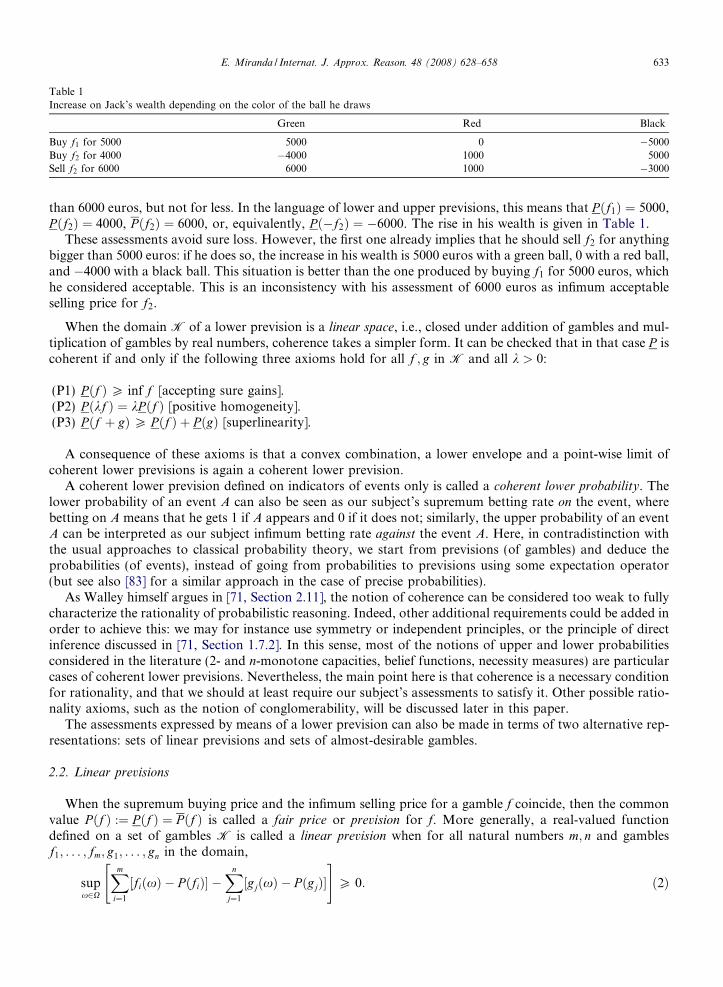
Table 1Increase on Jack’s wealth depending on the color of the ball he draws

Green Red Black

Buy f1 for 5000 5000 0 �5000Buy f2 for 4000 �4000 1000 5000Sell f2 for 6000 6000 1000 �3000


than 6000 euros, but not for less. In the language of lower and upper previsions, this means that P ðf1Þ ¼ 5000,P ðf2Þ ¼ 4000, P ðf2Þ ¼ 6000, or, equivalently, P ð�f2Þ ¼ �6000. The rise in his wealth is given in Table 1.

These assessments avoid sure loss. However, the first one already implies that he should sell f2 for anythingbigger than 5000 euros: if he does so, the increase in his wealth is 5000 euros with a green ball, 0 with a red ball,and �4000 with a black ball. This situation is better than the one produced by buying f1 for 5000 euros, whichhe considered acceptable. This is an inconsistency with his assessment of 6000 euros as infimum acceptableselling price for f2.

When the domain K of a lower prevision is a linear space, i.e., closed under addition of gambles and mul-tiplication of gambles by real numbers, coherence takes a simpler form. It can be checked that in that case P iscoherent if and only if the following three axioms hold for all f ; g in K and all k > 0:

(P1) P ðf ÞP inf f [accepting sure gains].(P2) P ðkf Þ ¼ kP ðf Þ [positive homogeneity].(P3) P ðf þ gÞP P ðf Þ þ PðgÞ [superlinearity].

A consequence of these axioms is that a convex combination, a lower envelope and a point-wise limit ofcoherent lower previsions is again a coherent lower prevision.

A coherent lower prevision defined on indicators of events only is called a coherent lower probability. Thelower probability of an event A can also be seen as our subject’s supremum betting rate on the event, wherebetting on A means that he gets 1 if A appears and 0 if it does not; similarly, the upper probability of an eventA can be interpreted as our subject infimum betting rate against the event A. Here, in contradistinction withthe usual approaches to classical probability theory, we start from previsions (of gambles) and deduce theprobabilities (of events), instead of going from probabilities to previsions using some expectation operator(but see also [83] for a similar approach in the case of precise probabilities).

As Walley himself argues in [71, Section 2.11], the notion of coherence can be considered too weak to fullycharacterize the rationality of probabilistic reasoning. Indeed, other additional requirements could be added inorder to achieve this: we may for instance use symmetry or independent principles, or the principle of directinference discussed in [71, Section 1.7.2]. In this sense, most of the notions of upper and lower probabilitiesconsidered in the literature (2- and n-monotone capacities, belief functions, necessity measures) are particularcases of coherent lower previsions. Nevertheless, the main point here is that coherence is a necessary conditionfor rationality, and that we should at least require our subject’s assessments to satisfy it. Other possible ratio-nality axioms, such as the notion of conglomerability, will be discussed later in this paper.

The assessments expressed by means of a lower prevision can also be made in terms of two alternative rep-resentations: sets of linear previsions and sets of almost-desirable gambles.

2.2. Linear previsions

When the supremum buying price and the infimum selling price for a gamble f coincide, then the commonvalue P ðf Þ :¼ P ðf Þ ¼ P ðf Þ is called a fair price or prevision for f. More generally, a real-valued functiondefined on a set of gambles K is called a linear prevision when for all natural numbers m; n and gamblesf1; . . . ; fm; g1; . . . ; gn in the domain,

supx2X

Xm

i¼1

½fiðxÞ � PðfiÞ� �Xn

j¼1

½gjðxÞ � P ðgjÞ�" #

P 0: ð2Þ


Assume that this condition does not hold for certain gambles f1; . . . ; fm; g1; . . . ; gn in K. Then there existssome d > 0 such that

g1

g2

g3

g4

Xm

i¼1

½fiðxÞ � P ðfiÞ þ d� þXn

j¼1

½P ðgjÞ � gj þ d� < �d ð3Þ

for all x 2 X. Since P ðfiÞ is our subject’s supremum acceptable buying price for the gamble fi, he is disposed topay P ðfiÞ � d for it, so the transaction fi � P ðfiÞ þ d is acceptable for him; on the other hand, since PðgjÞ is hisinfimum acceptable selling price for gj, he is disposed to sell it for the price PðgjÞ þ d, so the transactionPðgjÞ þ d� gj is acceptable. But Eq. (3) tells us that the sum of these acceptable transactions produces a lossof at least d, no matter the outcome of the experiment!

A linear prevision P is coherent, both when interpreted as a lower and as an upper prevision; the formermeans that P :¼ P is a coherent lower prevision on K, the latter that the functional P 1 on�K :¼ f�f : f 2Kg given by P 1ðf Þ ¼ �Pð�f Þ is a coherent lower prevision on �K. However, not everyfunctional which is coherent both as a lower and as an upper prevision is a linear prevision. This is becausecoherence as a lower prevision only guarantees that Eq. (2) holds for n 6 1, and coherence as an upper pre-vision only guarantees that the same equation holds for the case where m 6 1. An example showing that thesetwo properties do not imply that Eq. (2) holds for all non-negative natural numbers n;m is the following:

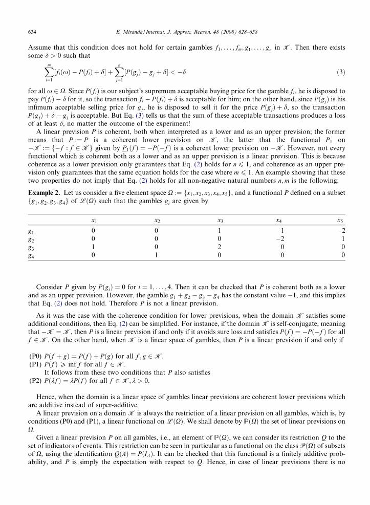
Example 2. Let us consider a five element space X :¼ fx1; x2; x3; x4; x5g, and a functional P defined on a subsetfg1; g2; g3; g4g of LðXÞ such that the gambles gi are given by

x1 x2 x3 x4 x5

0 0 1 1 �20 0 0 �2 11 0 2 0 00 1 0 0 0

Consider P given by P ðgiÞ ¼ 0 for i ¼ 1; . . . ; 4. Then it can be checked that P is coherent both as a lowerand as an upper prevision. However, the gamble g1 þ g2 � g3 � g4 has the constant value �1, and this impliesthat Eq. (2) does not hold. Therefore P is not a linear prevision.

As it was the case with the coherence condition for lower previsions, when the domain K satisfies someadditional conditions, then Eq. (2) can be simplified. For instance, if the domain K is self-conjugate, meaningthat �K ¼K, then P is a linear prevision if and only if it avoids sure loss and satisfies Pðf Þ ¼ �Pð�f Þ for allf 2K. On the other hand, when K is a linear space of gambles, then P is a linear prevision if and only if

(P0) P ðf þ gÞ ¼ P ðf Þ þ P ðgÞ for all f ; g 2K.(P1) P ðf ÞP inf f for all f 2K.

It follows from these two conditions that P also satisfies(P2) P ðkf Þ ¼ kPðf Þ for all f 2K; k > 0.

Hence, when the domain is a linear space of gambles linear previsions are coherent lower previsions whichare additive instead of super-additive.

A linear prevision on a domain K is always the restriction of a linear prevision on all gambles, which is, byconditions (P0) and (P1), a linear functional on LðXÞ. We shall denote by PðXÞ the set of linear previsions onX.

Given a linear prevision P on all gambles, i.e., an element of PðXÞ, we can consider its restriction Q to theset of indicators of events. This restriction can be seen in particular as a functional on the class PðXÞ of subsetsof X, using the identification QðAÞ ¼ PðIAÞ. It can be checked that this functional is a finitely additive prob-ability, and P is simply the expectation with respect to Q. Hence, in case of linear previsions there is no


difference in expressive power between representing the information in terms of events or in terms of gambles:the restriction to events (the probability) determines the value on gambles (the expectation) and vice versa.This is no longer true in the imprecise case, where there usually are infinitely many coherent extensions ofa coherent lower probability [71, Section 2.7.3], and this is why the theory is formulated in general in termsof gambles. The fact that lower previsions of events do not determine uniquely the lower previsions of gamblesis due to the fact that we are not dealing with additive functionals anymore.

A linear prevision P whose domain is made up of the indicators of the events in some class A is called anadditive probability on A. If in particular A is a field of events, then P is a finitely additive probability in theusual sense, and moreover condition 2 simplifies to the usual axioms of finite additivity:

(a) P ðAÞP 0 for all A in A.(b) P ðXÞ ¼ 1.(c) P ðA [ BÞ ¼ PðAÞ þ P ðBÞ whenever A \ B ¼ ;.

Example 1(cont.). Assume that Jack knows that there are only 10 balls in the urn, and that the drawing is fair,so that the probability of each color depends only on the proportion of balls of that color. If he knew the exactcomposition of the urn, for instance that there are five green balls, four red balls and one black ball, then hisexpected gain with the gamble f1 would be 0:5 � 10000 þ 0:4 � 5000� 0:1 � 0 ¼ 7000 euros, and this should behis fair price for the gamble. Any linear prevision will be determined by its restriction to events via theexpectation operator. This restriction to events corresponds to some particular composition of the urn: if heknows that there are four red balls out of 10 in the urn, then his betting rate on or against drawing a red ball(that is, his fair price for a gamble with reward 1 if he draws a red ball and 0 if he does not) should be 0.4.

We can characterize the coherence of a lower prevision P with domain K by means of its set of dominating

linear previsions, which we shall denote as

4 Re(has thwill nodecisio

MðPÞ :¼ fP 2 PðXÞ : P ðf ÞP P ðf Þ for all f in Kg:
It can be checked that P is coherent if and only if it is the lower envelope of MðP Þ, that is, if and only if
P ðf Þ ¼ minfP ðf Þ : P 2MðP Þg
for all f in K. Moreover, the set of dominating linear previsions allows us to establish a one-to-one correspon-dence between coherent lower previsions P and closed (in the weak-* topology) and convex sets of linear pre-visions: given a coherent lower prevision P we can consider the (closed and convex) set of linear previsionsMðP Þ. Conversely, every closed and convex set M of linear previsions determines uniquely a coherent lowerprevision P by taking lower envelopes.4 Besides, it can be checked that these two operations (taking lowerenvelopes of closed convex sets of linear previsions and considering the linear previsions that dominate a givencoherent lower prevision) commute. We should warn the reader, however, that this equivalence does not holdin general for the conditional lower previsions that we shall introduce in Section 3, although there exists anenvelope result for the alternative approach developed by Williams that we shall present in Section 5.2.
The representation of coherent lower previsions in terms of sets of linear previsions allows us to give them aBayesian sensitivity analysis representation: we may assume that there is a fair price for every gamble f on X,which results on a linear prevision P 2 PðXÞ, and such that our subject’s imperfect knowledge of P only allowshim to place it among a set of possible candidates, M. Then the inferences he can make from M are equivalentto the ones he can make using the lower envelope P of this set. This lower envelope is a coherent lower prevision.

Hence, all the developments we make with (unconditional) coherent lower previsions can also be made withsets of finitely additive probabilities, or equivalently with the set of their associated expectation operators,which are linear previsions. In this sense, there is a strong link between this theory and robust Bayesian anal-

mark nonetheless that convexity is not really an issue here, since a set of linear previsions represents the same behavioral dispositionse same lower and upper envelopes) as its convex hull, and in many cases, the set of linear previsions compatible with some beliefst be convex; see [10,13] for more details, and [55] for a more critical approach to the assumption of convexity in the context ofn making.


ysis [53]. We shall see in Section 3 that, roughly speaking, this link only holds when we update our informationif we deal with finite sets of categories.

Example 1(cont.). The lower previsions P ðf1Þ ¼ 5000 and P ðf2Þ ¼ 4000 that Jack established before for thegambles f1; f2 are coherent. The information P gives is equivalent to its set of dominating linear previsions,MðP Þ. Any of these linear previsions is characterized by its restriction to events, which gives the probability ofdrawing a ball of some particular color. In this case, it can be checked that

TableThe pr

P(Gre

00.10.10.20.20.20.30.30.40.40.50.5

MðP Þ :¼ fðp1; p2; p3Þ : p1 P p3; p2 P 4ðp1 � p3Þ � p3g;
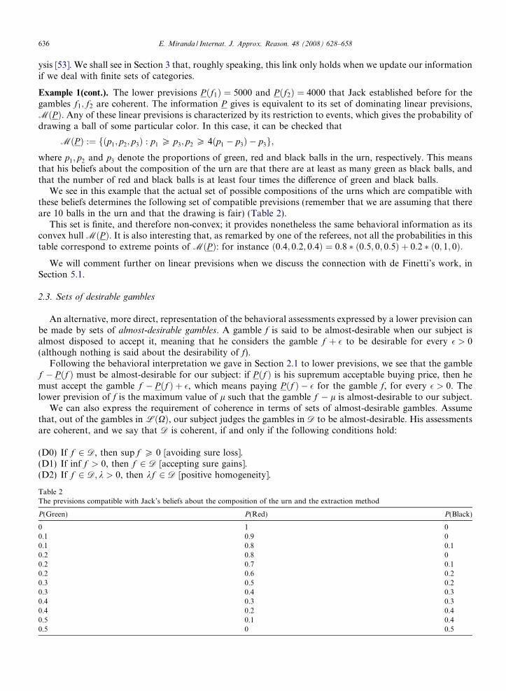
where p1; p2 and p3 denote the proportions of green, red and black balls in the urn, respectively. This meansthat his beliefs about the composition of the urn are that there are at least as many green as black balls, andthat the number of red and black balls is at least four times the difference of green and black balls.
We see in this example that the actual set of possible compositions of the urns which are compatible withthese beliefs determines the following set of compatible previsions (remember that we are assuming that thereare 10 balls in the urn and that the drawing is fair) (Table 2).

This set is finite, and therefore non-convex; it provides nonetheless the same behavioral information as itsconvex hull MðP Þ. It is also interesting that, as remarked by one of the referees, not all the probabilities in thistable correspond to extreme points of MðP Þ: for instance ð0:4; 0:2; 0:4Þ ¼ 0:8 � ð0:5; 0; 0:5Þ þ 0:2 � ð0; 1; 0Þ:

We will comment further on linear previsions when we discuss the connection with de Finetti’s work, inSection 5.1.

2.3. Sets of desirable gambles

An alternative, more direct, representation of the behavioral assessments expressed by a lower prevision canbe made by sets of almost-desirable gambles. A gamble f is said to be almost-desirable when our subject isalmost disposed to accept it, meaning that he considers the gamble f þ � to be desirable for every � > 0(although nothing is said about the desirability of f).

Following the behavioral interpretation we gave in Section 2.1 to lower previsions, we see that the gamblef � P ðf Þ must be almost-desirable for our subject: if P ðf Þ is his supremum acceptable buying price, then hemust accept the gamble f � P ðf Þ þ �, which means paying Pðf Þ � � for the gamble f, for every � > 0. Thelower prevision of f is the maximum value of l such that the gamble f � l is almost-desirable to our subject.

We can also express the requirement of coherence in terms of sets of almost-desirable gambles. Assumethat, out of the gambles in LðXÞ, our subject judges the gambles in D to be almost-desirable. His assessmentsare coherent, and we say that D is coherent, if and only if the following conditions hold:

(D0) If f 2 D, then sup f P 0 [avoiding sure loss].(D1) If inf f > 0, then f 2 D [accepting sure gains].(D2) If f 2 D; k > 0, then kf 2 D [positive homogeneity].

2evisions compatible with Jack’s beliefs about the composition of the urn and the extraction method

en) P(Red) P(Black)

1 00.9 00.8 0.10.8 00.7 0.10.6 0.20.5 0.20.4 0.30.3 0.30.2 0.40.1 0.40 0.5


(D3) If f ; g 2 D, then f þ g 2 D [addition].(D4) If f þ d 2 D for all d > 0, then f 2 D [closure].

Let us give an interpretation of these axioms. D0 states that a gamble f which makes him lose utiles, nomatter the outcome, should not be acceptable for our subject. D1 on the other hand tells that he should accepta gamble which will always increase his wealth. D2 means that the almost desirability of a gamble f should notdepend on the scale of utility we are considering. D3 states that if two gambles f and g are almost-desirable,our subject should be disposed to accept their combined transaction. Axioms D0–D3 characterize the so-calleddesirable gambles (see [71, Section 2.2.4]). A class of desirable gambles is always a convex cone of gambles.Axiom D4 is a closure property, and allows us to give an interpretation in terms of almost-desirability.

It is a consequence of axioms (D1) and (D4) that any non-negative gamble f is almost-desirable. From thisand (D3), we can deduce that if a gamble f dominates an almost-desirable gamble g, then f (which is the sum ofthe almost-desirable gambles g and f � g) is also almost-desirable. Finally, it follows from (D2) and (D3) thata positive linear combination of almost-desirable gambles is also almost-desirable. These are the rationalityrequirements we have used in Section 2.1 to justify the notion of coherence.

A coherent set of almost-desirable gambles is a closed convex cone containing all non-negative gambles andnot containing any uniformly negative gambles. There is, moreover, a one-to-one correspondence betweencoherent lower previsions on LðXÞ and coherent sets of almost-desirable gambles: given a coherent lower pre-vision P on LðXÞ, the class

DP :¼ ff 2LðXÞ : P ðf ÞP 0g ð4Þ
is a coherent set of almost-desirable gambles. Conversely, if D is a coherent set of almost-desirable gambles,the lower prevision PD given by
PDðf Þ :¼ maxfl : f � l 2 Dg ð5Þ
is coherent. Moreover, it can be checked that the operations given in Eqs. (4) and (5) commute, meaning that ifwe consider a coherent lower prevision P on LðXÞ and the set DP of almost-desirable gambles that we canobtain from it via Eq. (4), then the lower prevision PDP that we define on LðXÞ by Eq. (5) coincides withP ; and similarly if we start with a set of almost-desirable gambles.
Since the assessments expressed by means of a coherent lower prevision P can also be expressed by means ofits set of dominating linear previsions MðP Þ, we see that this set is also equivalent to the set of almost-desirablegambles D we have just derived. Indeed, given a coherent set of almost-desirable gambles D, we can considerthe set of linear previsions

MD :¼ fP 2 PðXÞ : P ðf ÞP 0 for all f in Dg:
MD is a closed and convex set of linear previsions, and its lower envelope P coincides with the coherent lowerprevision induced by D through Eq. (5).
Conversely, given a closed and convex set of linear previsions M, we can consider the set of gambles

DM ¼ ff 2LðXÞ : P ðf ÞP 0 for all P in Mg:
DM is a coherent set of almost-desirable gambles, and the lower prevision PDM
it induces is equal to the lowerenvelope of M.

Example 1(cont.). From the set of linear previsions MðP Þ compatible with Jack’s coherent assessments, weobtain the class of almost-desirable gambles

D ¼ fða1; a2; a3Þ : a1 þ a3 P 0; a2 P 0; a1 P maxf�4a2;�3ða1 þ a2 þ a3Þ;�a2 � 4ða1 þ a3Þgg;

where a1 ¼ f ðgreenÞ; a2 ¼ f ðredÞ; a3 ¼ f ðblackÞ:

Hence, we have three equivalent representations of coherent assessments: coherent lower previsions, closedand convex sets of linear previsions, and coherent sets of almost-desirable gambles. The use of one or anotherof these representations will depend on the context: for instance, a representation in terms of sets of linear pre-visions may be more useful if we want to give our model a Bayesian sensitivity analysis interpretation, while theuse of sets of almost-desirable gambles may be more interesting in connection when decision making.


Note however that these representations do not tell us anything about our subject’s buying behavior for thegambles f at the price P ðf Þ: he may accept it, as he does for the price P ðf Þ � � for all � > 0, but then he also mightnot. If we want to give information about the behavior for P ðf Þ, we have to consider a more informative model: setsof really desirable gambles. These sets allow to distinguish between desirability and almost desirability, and theysolve moreover some of the difficulties we shall see in Section 3 when talking about conditioning on sets of prob-ability zero [77]. We refer to [71, Appendix F] and [20,77] for a more detailed account of this more general model.

2.4. Natural extension

Assume now that our subject has established his acceptable buying prices rates for all gambles on somedomain K. He may then wish to check which are the consequences of these assessments for other gambles.If for instance he is disposed to pay a price l1 for a gamble f1 and a price l2 for a gamble f2, he should bedisposed to pay at least the price l1 þ l2 for their sum f1 þ f2. In general, given a gamble f which is not inthe domain, he would like to know which is the supremum buying price that he should find acceptable forf, taking into account his previous assessments ðP Þ, and using only the condition of coherence.

Assume that for a given price l there exist gambles g1; . . . ; gn in K and non-negative real numbersk1; . . . ; kn, such that

f ðxÞ � l PXn

i¼1

kiðgiðxÞ � P ðgiÞÞ:

Since all the transactions in the sum of the right-hand side are acceptable to him, so should be the left-handside, which dominates their sum. Hence, he should be disposed to pay the price l for the gamble f, and there-fore his supremum acceptable buying price should be greater than or equal to l. To use the language of theprevious section, the right-hand side of the inequality is an almost-desirable gamble, and as a consequence somust be the gamble on the left-hand side. And the correspondence between almost-desirable gambles andcoherent lower previsions implies then that the lower prevision of f should be greater than, or equal to, l.

The lower prevision that provides these supremum acceptable buying prices is called the natural extension

of P . It is given, for f 2LðXÞ, by

Eðf Þ ¼ supgi2K;kiP0;

i¼1;...;ni ;ni2N

infx2X

f ðxÞ �Xn

i¼1

ki½giðxÞ � P ðgiÞ�( )

: ð6Þ

The reasoning above tells us that our subject should be disposed to pay the price Eðf Þ � � for the gamble f, andthis for every � > 0. Hence, his supremum acceptable buying price should dominate Eðf Þ. But we can checkalso that this value is sufficient to achieve coherence [71, Theorem 3.1.2].

Therefore, Eðf Þ is the smallest, or more conservative, value we can give to the buying price of f in order toachieve coherence with the assessments in P . There may be other coherent extensions, which may be interest-ing in some situations; however, any other of these less conservative, coherent extensions will represent stron-ger assessments than the ones that can be derived purely from P and the notion of coherence. This is why weusually adopt E as our inferred model.

Coherent lower previsions constitute a very general model for uncertainty: they include for instance as par-ticular cases 2- and n-monotone capacities, belief functions, or probability measures. In this style, the procedureof natural extension includes as particular cases many of the extension procedures present in the literature:Choquet integration of 2- and n-monotone capacities, Lebesgue integration of probability measures, or Bayes’srule for updating probability measures. It provides the consequences for other gambles of our previous assess-ments and the notion of coherence. If for instance we consider a probability measure on some r-field of eventsA, the natural extension to all events will determine the set of finitely additive extensions of P to PðXÞ, and itwill be equal to the lower envelope of this set. It coincides moreover with the inner measure of P.

Example 1(cont.). Jack is offered next a new gamble f3, whose reward is 2000 euros if he draws a green ball,3000 if he draws a red ball, and 4000 euros if he draws a black ball. Taking into account his previousassessments, P ðf1Þ ¼ 5000; Pðf2Þ ¼ 4000, he should at least pay


Eðf3Þ ¼ supk1;k2P0

minf2000� 5000k1 þ 4000k2; 3000� 1000k2; 4000þ 5000k1 � 5000k2g:

It can be checked that this supremum is achieved for k1 ¼ 0; k2 ¼ 0:2. We obtain then Eðf3Þ ¼ 2800. This is thesupremum acceptable buying price for f3 that Jack can derive from his previous assessments and the notion ofcoherence.

If the lower prevision P does not avoid sure loss, then Eq. (6) yields Eðf Þ ¼ 1 for all f 2LðXÞ. The idea isthat if our subject’s initial assessments are such that he can end up losing utiles no matter the outcome of theexperiment, he will also lose utiles with any other gamble that they offer to him. Because of this, the first thingwe have to verify is whether the initial assessments avoid sure loss, and only then we can consider their con-sequences on other gambles.

When P avoids sure loss, E is the smallest coherent lower prevision on all gambles that dominates P on K,in the sense that E is coherent and any other coherent lower prevision E0 on LðXÞ such that E0ðf ÞP P ðf Þ forall f 2K will satisfy E0ðf ÞP Eðf Þ for all f in LðXÞ. E is not in general an extension of P ; it will only be sowhen P is coherent itself. Otherwise, the natural extension will correct the assessments present in P into thesmallest possible coherent lower prevision. Hence, the notion of natural extension can be used to modifythe initial assessments into other assessments that satisfy the notion of coherence, and it does so in theleast-committal way, i.e., it provides the smallest coherent lower prevision with the same property.

Example 1(cont.). Let us consider again the assessments P ðf1Þ ¼ 5000, P ðf2Þ ¼ 4000 and P ðf2Þ ¼ 6000. Theseimply the acceptable buying transactions in Table 1, which, as we showed, avoid sure loss but are incoherent.If we apply Eq. (6) to them we obtain that their natural extension is Eðf1Þ ¼ 5000, Eðf2Þ ¼ 4000, Eðf2Þ ¼ 5000.Hence, it is a consequence of coherence that Jack should be disposed to sell the gamble f2 for anything biggerthan 5000 euros.

The natural extension of the assessments given by a coherent lower prevision P can also be calculated interms of the equivalent representations we have given in Sections 2.2 and 2.3.

Consider a coherent lower prevision P with domain K, and let DP be the set of almost-desirable gamblesassociated with the lower prevision P by Eq. (4):

DP :¼ ff 2K : P ðf ÞP 0g:

The natural extension EDP of DP provides the smallest set of almost-desirable gambles that contains DP and iscoherent. It is the closure (in the supremum norm topology) of

f : 9fj 2 DP ; kj > 0 such that f PXn

j¼1

kjfj

( ); ð7Þ

which is the smallest convex cone that contains DP and all non-negative gambles. Then the natural extensionof P to all gambles is given by

Eðf Þ ¼ supfl : f � l 2 EDP g:

If we consider the set MðP Þ of linear previsions that dominate P on K, then

Eðf Þ ¼ minfP ðf Þ : P 2MðP Þg: ð8Þ
This last expression also makes sense if we consider the Bayesian sensitivity analysis interpretation we havegiven to coherent lower previsions in Section 2.2: there is a linear prevision modelling our subject’s informa-tion, but his imperfect knowledge of it makes him consider a set of linear previsions MðPÞ, whose lower enve-lope is P . If he wants to extend P to a bigger domain, he should consider all the linear previsions in MðP Þ aspossible models (he has no additional information allowing to disregard any of them), or equivalently theirlower envelope. He obtains then that MðP Þ ¼MðEÞ.
The procedure of natural extension preserves the equivalence between the different representations of ourassessments: if we consider for instance a coherent lower prevision P withK and the set of almost-desirable gam-bles DP we derive from Eq. (4), then we can consider the natural extension of DP via Eq. (7). The coherent lowerprevision we can derive from this set of acceptable gambles using Eq. (5) coincides with the natural extension E of


P . This is because the notion of natural extension, both for lower or linear previsions or for sets of desirable gam-bles determines the least-committal extension of our initial model that satisfies the notion of coherence.

On the other hand, we can also consider the natural extension of a lower prevision P from a domain K to abigger domain K1 (not necessarily equal to LðXÞ). It can be checked then that the procedure of natural exten-sion is transitive, in the following sense: if E1 denotes the natural extension of P to K1 and we later considerthe natural extension E2 of E1 to some bigger domain K2 �K1, then E2 agrees with the natural extension of Pfrom K to K2: in both cases we are only considering the behavioral consequences of the assessments on Kand the condition of coherence. This is easiest to see using Eq. (8): we have MðE1Þ ¼MðE2Þ ¼MðP Þ.

3. Updating and combining information

So far, we have assumed that the only information that our subject possesses about the outcome of theexperiment is that it belongs to the set X. But it may happen that, after he has made his assessments, he comesto have some additional information about this outcome, for instance that it belongs to some element of apartition B of X. He then has to update his assessments, and the way to do this is by means of what we shallcall conditional lower previsions.

3.1. Conditional lower previsions

Let B be a subset of the sampling space X, and consider a gamble f on X. Walley’s theory of coherent lowerprevisions gives two different interpretations of Pðf jBÞ: the updated and the contingent one. The most naturalin our view is the contingent interpretation, under which P ðf jBÞ is our subject’s current supremum buyingprice for the gamble f contingent on B, that is, the supremum value of l such that the gamble IBðf � lÞ isdesirable for our subject.

In order to relate our subject’s current dispositions on a gamble f contingent on B with his dispositionstowards this gamble if he later shall come to know whether the outcome of the experiment belongs to B, Wal-ley introduces the so-called updating principle. We say a gamble f is B-desirable for our subject when he is cur-rently disposed to accept f provided he later observes that the outcome belongs to B. Then the updatingprinciple requires that a gamble is B-desirable if and only if IBf is desirable. In this way, we can relate thecurrent and future dispositions of our subject.

Under the updated interpretation of conditional lower previsions, P ðf jBÞ is the subject’s supremum accept-able buying price he would pay for the gamble f now if he came to know later that the outcome belongs to theset B, and nothing more. It coincides with the value determined by the contingent interpretation of Pðf jBÞbecause of the updating principle.

Let B be a partition of our sampling space, X, and consider an element B of this partition. This partitioncould be for instance a class of categories of the set of outcomes. Assume that our subject has given condi-tional assessments P ðf jBÞ for all gambles f on some domain HB. As it was the case for (unconditional) lowerprevisions, we should require that these assessments are consistent with each other. We say that the condi-tional lower prevision P ð�jBÞ is separately coherent when the following two conditions are satisfied:

(SC1) It is coherent as an unconditional prevision, i.e.,

supx2X

Xn

i¼1

½fiðxÞ � PðfijBÞ� � m½f0ðxÞ � P ðf0jBÞ�P 0 ð9Þ

for all non-negative integers n;m and all gambles f0; . . . ; fn in HB;(SC2) the indicator function of B belongs to HB and P satisfies P ðBjBÞ ¼ 1.

The coherence requirement (9) can be given a behavioral interpretation in the same way as with (uncondi-tional) coherence in Eq. (1): if it does not hold for some non-negative integers n;m and gambles f0; . . . ; fn inHB, then it can be checked that either: (i) the almost-desirable gamble

Pni¼1½fi � P ðfijBÞ� incurs in a sure loss

(if m ¼ 0) or (ii) we can raise Pðf0jBÞ in some positive quantity d, contradicting our interpretation of it as hissupremum acceptable buying price (if m > 0).


On the other hand, Eq. (9) already implies that P ðBjBÞ should be smaller than, or equal to, 1. That werequire it to be equal to one means just that our subject should bet at all odds on the occurrence of the eventB after having observed it.

In this way, we can obtain separately coherent conditional lower previsions P ð�jBÞ with domains HB for allevents B in the partition B. It is a consequence of separate coherence that the conditional lower previsionP ðf jBÞ does only depend on the values that f takes on B, i.e, for every two gambles f and g such thatf ðxÞ ¼ gðxÞ for all x 2 B, we should have P ðf jBÞ ¼ P ðgjBÞ. This property implies that all the domains HB

can be extended to the common domain H :¼ ff ¼P

B2BfB : fB 2HB 8Bg, and we can define on H a con-

ditional lower prevision P ð�jBÞ by

5 Thfor mo

P ðf jBÞ :¼XB2B

IBP ðf jBÞ;

i.e., the gamble on X that assumes the value P ðf jBÞ on all elements of B. This conditional lower prevision isthen called separately coherent when P ð�jBÞ is separately coherent for all B 2 B. It provides the updated supre-mum buying price after learning that the outcome of the experiment belongs to some particular element of B.We shall later use the notation

Gðf jBÞ :¼ IBðf � P ðf jBÞÞ; Gðf jBÞ :¼XB2B

Gðf jBÞ ¼ f � Pðf jBÞ: ð10Þ

When the domain H of Pð�jBÞ is a linear space containing all constant gambles, then separate coherence isequivalent to:

(C1) P ðf jBÞP infx2Bf ðxÞ.(C2) P ðkf jBÞ ¼ kP ðf jBÞ.(C3) P ðf þ gjBÞP P ðf jBÞ þ P ðgjBÞ

for all positive real k;B 2 B and gambles f ; g in H. The first requirement shows that the conditional lowerprevision on B should only depend on the behavior of f on this set; conditions (C2) and (C3) are the counter-parts of the requirements (P2) and (P3) we made for unconditional lower previsions, respectively.

Example 1(cont.). For the gambles f1 and f2 whose reward in terms of the color of the ball drawn is given inTable 3.

Jack had established the coherent assessments Pðf1Þ ¼ 5000 and P ðf2Þ ¼ 4000. But he may also establishnow his supremum acceptable buying prices for these gambles depending on some future information on thecolor of the ball drawn. If for instance he is informed that the ball drawn is not green, Jack should update hislower prevision for the gamble f2, because he is sure that in that case he would get at least a prize of 5000 eurosout of it. On the other hand, if he keeps the supremum buying prize of 5000 euros for f1 he is implying that heis sure that the ball that has been drawn is red once he comes to know that it is not green.

If for instance he considers as possible models the ones in Table 2 and updates them using Bayes’s rule, thenthe updated supremum buying prices he should give by taking lower envelopes would be P ðf1jnot greenÞ ¼ 0and P ðf2jnot greenÞ ¼ 5000.5

3.2. Coherence of a finite number of conditional lower previsions

In practice, it is not uncommon to have lower previsions conditional on different partitions B1; . . . ;Bn of X.We can think for instance of different sets of categories, or of information provided in a sequential way. Weend up then with a finite number of conditional lower previsions P ð�jB1Þ; . . . ; P ð�jBnÞ with respective domainsH1; . . . ;Hn �LðXÞ, which we shall assume are separately coherent.

is is an instance of a procedure called regular extension, that can sometimes be used to coherently update beliefs; see [71, Appendix J]re details.

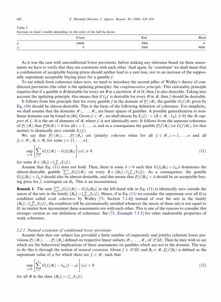
Table 3Increase on Jack’s wealth depending on the color of the ball he draws

Green Red Black

f1 10000 5000 0f2 0 5000 9000


As it was the case with unconditional lower previsions, before making any inference based on these assess-ments we have to verify that they are consistent with each other. And again, by ‘consistent’ we shall mean thata combination of acceptable buying prices should neither lead to a sure loss, nor to an increase of the suppos-edly supremum acceptable buying price for a gamble f.

To see which form coherence takes now, we need to introduce the second pillar of Walley’s theory of con-ditional previsions (the other is the updating principle): the conglomerative principle. This rationality principlerequires that if a gamble is B-desirable for every set B in a partition B of X, then f is also desirable. Taking intoaccount the updating principle, this means that if IBf is desirable for every B in B, then f should be desirable.

It follows from this principle that for every gamble f in the domain of P ð�jBÞ, the gamble Gðf jBÞ given byEq. (10) should be almost-desirable. This is the basis of the following definition of coherence. For simplicity,we shall assume that the domains H1; . . . ;Hn are linear spaces of gambles. A possible generalization to non-linear domains can be found in [46]. Given fi 2Hi, we shall denote by SiðfiÞ :¼ fB 2 Bi : IBfi 6¼ 0g the Bi-sup-

port of fi. It is the set of elements of Bi where fi is not identically zero. It follows from the separate coherenceof P ð�jBiÞ that P ð0jBiÞ ¼ 0 for all i ¼ 1; . . . ; n, and as a consequence the gamble P ðf jBiÞ (or Gðf jBiÞ, for thatmatter) is identically zero outside SiðfiÞ.

We say that P ð�jB1Þ; . . . ; P ð�jBnÞ are (jointly) coherent when for all fi 2Hi; i ¼ 1; . . . ; n and allf0 2Hj;B0 2 Bj for some j 2 f1; . . . ; ng,

supx2B

Xn

i¼1

GðfijBiÞ � Gðf0jB0Þ" #

ðxÞP 0 ð11Þ

for some B 2 fB0g [Sn

i¼1SiðfiÞ.Assume that Eq. (11) does not hold. Then, there is some d > 0 such that Gðf0jB0Þ þ IB0

d dominates thealmost-desirable gamble

Pni¼1GðfijBiÞ on every B 2 fB0g [

Sni¼1SiðfiÞ. As a consequence, the gamble

Gðf0jB0Þ þ IB0d should also be almost-desirable, and this means that P ðf jB0Þ þ d should be an acceptable buy-

ing price for f, contingent on B0. This is an inconsistency.

Remark 1. The sumPn

i¼1GðfijBiÞ � Gðf0jB0Þ� in the left-hand side in Eq. (11) is identically zero outside theunion of the sets in the family fB0g [

Sni¼1SiðfiÞ. Hence, if in Eq. (11) we consider the supremum over all X (a

condition called weak coherence by Walley [71, Section 7.1.4]) instead of over the sets in the familyfB0g [

Smi¼1SiðfiÞ, the condition will be automatically satisfied whenever the union of these sets is not equal to

X, no matter how inconsistent these assessments are with each other. This is one of the reasons to consider thisstronger version as our definition of coherence. See [71, Example 7.3.5] for other undesirable properties ofweak coherence.

3.2.1. Natural extension of conditional lower previsions

Assume then that our subject has provided a finite number of (separately and jointly) coherent lower pre-visions P ð�jB1Þ; . . . ; Pð�jBnÞ defined on respective linear subsets H1; . . . ;Hn of LðXÞ. Then he may wish to seewhich are the behavioral implications of these assessments on gambles which are not in the domain. The wayto do this is through the notion of natural extension. Given f 2LðXÞ and B0 2 Bi;Eðf jB0Þ is defined as thesupremum value of l for which there are fi 2Hi such that

supx2B

Xn

i¼1

GðfijBiÞ � IB0ðf � lÞ

" #ðxÞ < 0 ð12Þ

for all B in the class fB0g [ [ni¼1SiðfiÞ.


In the particular case where we only have an unconditional lower prevision, i.e., when n ¼ 1 and B1 ¼ fXg,this notion coincides with the unconditional natural extension we introduced in Section 2.4. If we have a num-ber of conditional lower previsions P ð�jB1Þ; . . . ; P ð�jBnÞ, we can calculate their natural extensionsEð�jB1Þ; . . . ;Eð�jBnÞ to all gambles using Eq. (12). If the partitions B1; . . . ;Bn are finite, then these naturalextensions share some of the properties of the unconditional natural extension:

1. They coincide with Pð�jB1Þ; . . . ; P ð�jBnÞ if and only if these conditional lower previsions are coherent.2. They are the smallest coherent extensions of P ð�jB1Þ; . . . ; P ð�jBnÞ to all gambles.3. They are the lower envelope of a family of coherent conditional linear previsions, fP cð�jB1Þ; . . . ;

P cð�jBnÞ : c 2 Cg.

Hence, when the partitions are finite, the notion of natural extension of a number of conditional lower pre-vision also provides us with the consequences of the assessments present on these previsions and the notion of(joint) coherence, to all gambles in the domain, and it can also be given a Bayesian sensitivity analysis inter-pretation. This is interesting for many applications, where we must deal with finite spaces only; however, thereare also interesting situations, such as parametric inference, where we must deal with infinite spaces and wherewe end up with partitions that have an infinite number of different elements. In that case, it is easy to see thatin order to achieve coherence, P ðf jB0Þ must be at least as large as the supremum l that satisfies Eq. (12) forsome fi 2Hi; i ¼ 1; . . . ; n. However, and unlike the case of finite partitions, we cannot guarantee that thesevalues provide coherent extensions of P ð�jB1Þ; . . . ; P ð�jBnÞ to all gambles: in general these will only be lowerbounds of all the coherent extensions. Indeed, when the partitions are infinite, we can have a number ofproblems:

1. There may be no coherent extensions, and as a consequence the natural extensions may not be coherent [71,Sections 6.6.6 and 6.6.7].

2. Even if the smallest coherent extensions exist, they may differ from the natural extensions, which are notcoherent [71, Section 8.1.3].

3. The minimal coherent extensions, and as a consequence also the natural extensions, may not be lower enve-lopes of coherent linear collections [71, Sections 6.6.9 and 6.6.10].

The natural extensions are the minimal coherent extensions of the lower previsions P ð�jB1Þ; . . . ; P ð�jBnÞ ifand only if they are jointly coherent themselves. But we need some additional conditions to guarantee the jointcoherence of Eð�jB1Þ; . . . ;Eð�jBnÞ. One of these conditions is that all the partitions Bi are finite. But even whenthe partitions are infinite it may happen that we are able to characterize the minimal coherent extensions, butthey differ from the natural extensions. One of the reasons for this defective behaviour of the natural extensionin the conditional case is the notion of conglomerability, that we shall treat in detail in the following section,and that becomes trivial in the case where the partitions are finite.

Example 3. An example where the natural extension fails to provide the minimal coherent extensions is givenin [48, Example 1]. Let us consider the possibility space X ¼ X1 �X2, where X1 ¼ X2 ¼ ½0; 1�, and thepartition B ¼ fBx1

: x1 2 X1g, where Bx1:¼ fx1g �X2. Let K ¼ fkp1 : k 2 Rg and H ¼ fgp2 : g 2LðX1Þg,

where the gamble kp1 is defined by kp1ðx1; x2Þ ¼ kx1, and the gamble gp2 by gp2ðx1; x2Þ ¼ gðx1Þx2. Let us definethe linear (and therefore coherent lower) prevision P on K by

P ðkp1Þ ¼ k;

and the conditional linear prevision P ð�jBÞ on H by

P ðgp2jBx1Þ ¼ gðx1Þ

for all x1 in X1. Then it can be checked that P and P ð�jBÞ are coherent. Given the gamble f on X, given by

f ðx1; x2Þ ¼0 if ðx1; x2Þ ¼ ð1� 1

n ; 1� 1nÞ for some n > 0;

1 otherwise;

�


it can be checked that the natural extension E of P ; P ð�jBÞ provides Eðf Þ ¼ 0. However, in this case the small-est coherent extensions M ;Mð�jBÞ of P ; P ð�jBÞ can be calculated, and we obtain Mðf Þ ¼ 1. The reason for thisdiscrepancy is that E only gives an extension of P which is coherent with P ð�jBÞ; if we also want to extendPð�jBÞ to all gambles the natural extension may not guarantee coherence.

This example provides an instance of the marginal extension of a number of conditional and unconditionallower previsions. When these previsions are conditioning on a sequence of increasingly finer partitions, themarginal extension can be used to determine the smallest coherent extensions to all gambles. See [71, Section6.7.2] and [48] for more information.

3.3. Coherence of an unconditional and a conditional lower prevision

Let us consider in more detail the case where we have a conditional lower prevision P ð�jBÞ on some domainH and an unconditional lower prevision P on some set of gambles K. Assume that they satisfy the followingconditions:

(a) K;H are linear subspaces of LðXÞ.(b) Given f 2H, the gambles P ðf jBÞ and IBf belong to H for all B 2 B.(c) P ð�jBÞ is separately coherent on H and P is coherent on K.

As Walley points out, the first two assumptions are made for mathematical convenience only; (b) can beassumed without loss of generality [71, Section 6.3.1], and the results can be extended to situations where(a) does not hold [46]. Note that the unconditional lower prevision can be seen as a conditional lower previsionby simply considering the partition {X}, and then Eq. (10) becomes Gðf Þ ¼ f � P ðf Þ.

The lower previsions P and P ð�jBÞ are jointly coherent, i.e., they satisfy Eq. (11), if and only if

(JC1) supx2X½Gðf1Þ þ Gðg1jBÞ � Gðf2Þ�P 0(JC2) supx2X½Gðf1Þ þ Gðg1jBÞ � Gðg2jB0Þ�P 0

for all f1; f2 2K; g1; g2 2H and B0 2 B. These conditions can be simplified under some additional assump-tions on the domains (see [71, Section 6.5] for details).

Again, it can be checked that if any of these conditions fails, the assessments of our subject produce incon-sistencies. Assume first that (JC1) does not hold. If f2 ¼ 0, then we have a sum of acceptable transactions thatproduces a sure loss. If f2 6¼ 0, then there is some d > 0 such that the gamble Gðf2Þ � d dominates the desirablegamble Gðf1Þ þ Gðg1jBÞ þ d. This means that our subject is willing to increase his supremum acceptable buy-ing price for f2 in d, a contradiction.

Similarly, if (JC2) does not hold and g2 ¼ 0 we have a sum of acceptable transactions that produces a sureloss; and if g2 6¼ 0 there is some d > 0 such that Gðg2jB0Þ � d dominates Gðf1Þ þ Gðg1jBÞ þ d and is thereforedesirable. Hence, our subject should be willing to pay P ðg2jB0Þ þ d for g2 contingent on B0, a contradiction.

It is a consequence of the joint coherence of P , P ð�jBÞ that, given f 2H and B 2 B;PðGðf jBÞÞ ¼ P ðIBðf � P ðf jBÞÞÞ ¼ 0, where Gðf jBÞ is defined in Eq. (10). When PðBÞ > 0, there is a uniquevalue l such that P ðIBðf � lÞÞ ¼ 0, and therefore this l must be the conditional lower prevision P ðf jBÞ. Thisis called the Generalised Bayes Rule (GBR). This rule has a number of interesting properties:

1. It is a generalization of Bayes’s rule in classical probability theory.2. If PðBÞ > 0 and we define P ðf jBÞ via the Generalized Bayes Rule, then it is the lower envelope of the con-

ditional linear previsions P ðf jBÞ that we can define using Bayes’s rule on the elements of MðP Þ.3. When the partition B is finite and P ðBÞ > 0 for all B 2 B, then the GBR uniquely determines the condi-

tional lower prevision P ð�jBÞ.

Example 4. Three horses (a, b and c) take part in a race. Our a priori lower probability for each horse beingthe winner is P ðfagÞ ¼ 0:1; P ðfbgÞ ¼ 0:25; P ðfcgÞ ¼ 0:3; Pðfa; bgÞ ¼ 0:4; P ðfa; cgÞ ¼ 0:6; P ðfb; cgÞ ¼ 0:7. Since


there are rumors that c is not going to take part in the race due to some injury, we may provide our updatedlower probabilities for that case using the Generalised Bayes Rule. Taking into account that we are dealingwith finite spaces and that the conditioning event has positive lower probability, applying the GeneralisedBayes Rule is equivalent to taking the lower envelope of the linear conditional previsions that we obtainapplying Bayes’s rule on the elements of MðP Þ. Thus, we obtain:

P ðfagjfa; bgÞ ¼ infP ðfagÞ

P ðfa; bgÞ : P 2MðP Þ� �

¼ 0:1=0:5 ¼ 0:2;

P ðfbgjfa; bgÞ ¼ infP ðfbgÞ

P ðfa; bgÞ : P 2MðP Þ� �

¼ 0:25=0:55 ¼ 0:45:

We saw in the previous section that a number of conditional lower previsions may be coherent and still havesome undesirable properties, when the partitions are infinite. Something similar applies to the case where wehave only a conditional and an unconditional lower prevision. For instance, a coherent pair P ; P ð�jBÞ is notnecessarily the lower envelope of coherent pairs of linear unconditional and conditional previsions, P ; P ð�jBÞ(these even may not exist). On the other hand, there are linear previsions P for which there is no conditionallinear prevision P ð�jBÞ such that P ; P ð�jBÞ are coherent in the sense of Eq. (11), i.e., linear previsions that can-not be updated in a coherent way to a linear conditional prevision P ð�jBÞ, but which can be updated to a con-ditional lower prevision.

Taking this into account, given an unconditional prevision P representing our subject’s beliefs and a par-tition B of X, he may be interested in considering the conditional lower previsions P ð�jBÞ which are coherentwith P , i.e., those for which conditions (JC1) and (JC2) are satisfied. A necessary and sufficient condition forthe existence of such P ð�jBÞ is that P is B-conglomerable: this is the case when given distinct sets B1;B2; . . . in Bsuch that P ðBnÞ > 0 for all n and a gamble f such that P ðIBn f ÞP 0 for all n, it holds that P ðI[nBn f ÞP 0.

The condition of B-conglomerability holds trivially when the partition B is finite, or when P ðBÞ ¼ 0 forevery set B in the partition. It only becomes non-trivial when we consider a partition B for which there areinfinitely many elements B satisfying P ðBÞ > 0. It makes sense as a rationality axiom once we accept the updat-ing and conglomerability principles: to see this, consider that if fBngn is a partition of X with P ðBnÞ > 0 andP ðIBn f ÞP 0, then for every d > 0 the gamble IBnðf þ dÞ is desirable. The updating and conglomerative prin-ciples imply then that f þ d is desirable, whence P ðf þ dÞP 0. Since this holds for all d > 0, we deduce thatP ðf ÞP 0.

More generally, Walley says that a coherent lower prevision P is fully conglomerable when it is B-conglo-merable for every partition B. A full conglomerable coherent lower prevision can be coherently updated to aconditional lower prevision P ð�jBÞ for any partition B of X. Again, full conglomerability can be accepted as anaxiom of rationality provided we accept the updating and conglomerability principles, and also provided thatwhen we define our coherent lower prevision we want to be able to updated for all possible partitions of our setof values.

There is an important connection between full conglomerability and countable additivity: given a linearprevision P on LðXÞ taking infinitely many values, it is fully conglomerable if and only for every countablepartition fBngn of X it satisfies

PnP ðBnÞ ¼ 1.

Full conglomerability is one of the points of disagreement between Walley’s and de Finetti’s work, that weshall present in more detail in Section 5.1. De Fintetti rejects the assumption of countable additivity on prob-abilities, and taking into account the above relationship also the property of full conglomerability. One keyobservation here is that de Finetti does not assume the conglomerative principle as a rationality axiom,and full conglomerability can be seen as a consequence of it.

When P is B-conglomerable and B 2 B, the conditional lower prevision P ðf jBÞ is uniquely determined bythe Generalised Bayes Rule if PðBÞ > 0. If P ðBÞ ¼ 0, however, there is not a unique value for P ðf jBÞ for whichwe achieve coherence. The smallest conditional lower prevision P ð�jBÞ which is coherent with P is the vacuousconditional prevision, given by Pðf jBÞ ¼ infx2Bf ðxÞ, and if we want to have more informative assessments wemay need some additional assumptions. Indeed, the approach to conditioning on sets of probability zero isone of the differences in the approach to conditioning by Walley (and also by de Finetti and Williams) andthat by Kolmogorov. In Kolmogorov’s approach, conditioning is made on a r-field A, and a conditional pre-


vision P ðf jAÞ is any A-measurable gamble which satisfies P ðgP ðf jAÞÞ ¼ P ðgf Þ for every A-measurable gam-ble g. In particular, if we consider an event B of probability zero, Kolmogorov allows the prevision P ð�jBÞ tobe completely arbitrary. Walley’s coherence condition is more general because it can be applied on previsionsconditional on partitions, and is more restrictive when dealing with sets of probability zero than Kolmogo-rov’s (although it may be argued that it also makes more sense). In particular, for a given linear previsionP there may not exist linear conditional previsions which are coherent with P.

One interesting approach to conditioning on sets of probability zero in a coherent setting is the use of zero-

layers by Coletti and Scozzafava [8, Chapter 12], which also appears in some earlier work by Krauss [38].Their approach to conditioning is nevertheless slightly different from Walley, since they consider conditionalprevisions as previsions whose domain is a class of conditional events. See [6–8] for further information onColetti and Scozzafava’s work, and [71, Section 6.10] and [78, Section 1.4] for further details on Walley’sapproach to conditioning on events of lower probability zero.

4. Independence

Next, we see how we can define the concept of independence in the context of coherent lower previsions. Letus consider two random variables X 1;X 2 taking values in respective sets X1;X2. In the classical setting, we callthe two variables (stochastically) independent when, given the probability measure P that models the valuethat ðX 1;X 2Þ assume jointly, any of the following conditions holds6

(a) P ðX 1 ¼ x1;X 2 ¼ x2Þ ¼ P ðX 1 ¼ x1Þ � P ðX 2 ¼ x2Þ for all x1 2 X1; x2 2 X2 [decomposition].(b) P ðX 1 ¼ x1jX 2 ¼ x2Þ ¼ P ðX 1 ¼ x1Þ for all x1 2 X1; x2 2 X2 [marginalization].

Remark 2. These two conditions are equivalent provided the marginal distributions are everywhere non-zero,that is, provided we are not conditioning on sets of probability zero. But if P ðX 2 ¼ x2Þ ¼ 0 for instance, thencondition (a) holds trivially, while there are many values of P ðX 1 ¼ x1jX 2 ¼ x2Þ for which condition (b) maynot hold, and this even under the more restrictive treatment of conditioning of sets of probability zero that wepresented in the previous section. To simplify this section, we shall assume throughout that the conditioningevents have all positive lower probability.

Provided we are conditioning on sets of positive probability, independence is a symmetrical notion: if (b)holds, then we also have

6 Indensity

7 Altcan be

P ðX 2 ¼ x2jX 1 ¼ x1Þ ¼ P ðX 2 ¼ x2Þ
for all x1 2 X1; x2 2 X2.
When our knowledge about the value that ðX 1;X 2Þ assume jointly is represented by means of a coherentlower prevision P on LðX1 �X2Þ, there is no unique way of extending the notion of independence. The prop-erties of decomposition and marginalization are no longer equivalent, and moreover symmetry is not immedi-ate anymore, meaning that we must distinguish between irrelevance (an asymmetrical notion) andindependence (its symmetric counterpart). On the other hand, all our definitions must be made in terms of vari-ables and not of events, since events do not keep all the information about the coherent lower prevision P .

In this section, we shall present some of the generalizations proposed in the literature and the relationshipsbetween them. To fix things, consider a coherent lower prevision P on LðX1 �X2Þ representing our knowl-edge about the value that X 1;X 2 assume jointly.7 We shall assume throughout that these two variables arelogically independent, meaning that the joint variable ðX 1;X 2Þ can assume any value in the product spaceX1 �X2. Our information about the random variable X 1 is given by the marginal lower prevision P 1, where

P 1ðf Þ ¼ Pðf Þ

this definition we assume that the sets X1;X2 are finite in order to simplify the notation; in the infinite case we would simply considerfunctions instead of probability mass functions. We also use X 1 ¼ x1 for denoting the event X�1

1 ðfx1gÞ to simplify the notation.hough here we are assuming for simplicity that the domain of P is LðX1 �X2Þ, all the developments we shall make in this sectiongeneralized to the case where the domain of P is some subset K of LðX1 �X2Þ.


for all f 2LðX1Þ, where f is the gamble given by f ðx1; x2Þ ¼ f ðx1Þ for all ðx1; x2Þ in X1 �X2 (such a gamble iscalled X1-measurable). Similarly, we can express our information about the outcome of X 2 by means of acoherent lower prevision P 2 on LðX2Þ, given by

P 2ðgÞ ¼ P ðgÞ
for all g 2LðX2Þ, where g is the gamble given by gðx1; x2Þ ¼ gðx2Þ for all ðx1; x2Þ in X1 �X2. We shall alsoassume that we have conditional lower previsions P ð�jX 1Þ; Pð�jX 2Þ on LðX1 �X2Þ such that P ; P ð�jX 1Þ andP ð�jX 2Þ are jointly coherent (i.e., they satisfy Eq. (11)). These conditional lower previsions represent our beliefsabout the outcome of one of the experiments provided we observe the outcome of the other. P ð�jX 1Þ is a lowerprevision conditional on the partition fX 1 ¼ x1 : x1 2 X1g of X, and similarly Pð�jX 2Þ is a lower prevision con-ditional on the partition fX 2 ¼ x2 : x2 2 X2g of X. To simplify the notation we shall sometimes use P ð�jx1Þ todenote P ð�jX 1 ¼ x1Þ and P ð�jx2Þ to denote P ð�jX 2 ¼ x2Þ for any x1 2 X1; x2 2 X2.
In the examples we shall consider in this section we shall deal with finite spaces only, and the conditioningevents shall always have positive lower probability; this will simplify the calculations of the conditional lowerprobabilities, because (i) they will be uniquely determined by the Generalised Bayes Rule and (ii) they will alsobe the lower envelope of the conditional precise probabilities that can be obtained by applying Bayes’s rule tothe set of compatible (precise) models.

4.1. Epistemic irrelevance

The first generalization of the concept of independence to imprecise probabilities is based on the margin-alization property, and is called epistemic irrelevance. We say that the experiment X 1 is epistemically irrelevant

for X 2 when our beliefs about the value that X 2 takes do not change after we learn the value that X 1 has taken.Formally, this holds if and only if

P ðf jX 1 ¼ x1Þ ¼ P 2ðf Þ

for all X2-measurable gambles f, and all x1 2 X1.The notion of epistemic irrelevance can also be defined in terms of sets of linear previsions [10,11]: we say

that X 1 is epistemically irrelevant for X 2 when

fP 2ð�jx1Þ : P 2 2MðPÞg ¼MðP 2Þ
for all x1 in X1, i.e., when learning the outcome about the first experiment does not change our uncertainty (theset of possible precise models) about the second experiment. Similarly, this notion can also be expressed interms of sets of desirable gambles: epistemic irrelevance means that the set of acceptable gambles for X 2 shouldnot change after learning the outcome of X 1 [49].
Example 5. We consider three urns with green and red balls. The first urn has one red ball and one green ball.In the second urn, we have two green balls, one red ball and two other balls of unknown color (they may bered or green). In the third urn, we have one green ball, two red balls and two other balls of unknown color.

We select a ball from the first urn. If it is green, then we select a ball from the second urn; if it is red, weselect a ball from the third urn. Let X 1 be the color of the first ball selected and X 2 the color of the second ball.We have

P ðthe second ball is greenjthe first ball is greenÞ ¼ 2=5;

P ðthe second ball is greenjthe first ball is redÞ ¼ 1=5

and thus the first experiment is not epistemically irrelevant to the second.

4.2. Epistemic independence

The notion of epistemic irrelevance is an asymmetric notion, meaning that X 1 can be epistemic irrelevantfor X 2 while X 2 is not epistemic irrelevant for X 1. When X 1 and X 2 are epistemically irrelevant to each other,we say that the two experiments are epistemically independent. This holds if and only if


P ðf jX 1 ¼ x1Þ ¼ P 2ðf Þ and P ðgjX 2 ¼ x2Þ ¼ P 1ðgÞ

for all X2-measurable gambles f ;X1-measurable gambles g; x1 2 X1, and x2 2 X2.In terms of sets of linear previsions, the notion of epistemic independence means that, for every x1 2 X1 and

x2 2 X2,

fP 2ð�jx1Þ : P 2 2MðP Þg ¼MðP 2Þ and fP 1ð�jx2Þ : P 1 2MðP Þg ¼MðP 1Þ:

The behavioral interpretation of these definitions is that our sets of desirable gambles for either experiment donot change after we learn the outcome of the other experiment.

Example 5(cont.). Assume now that in the third urn we also have two green balls, one red ball and two balls ofunknown color. We have

Pðthe second ball is greenjthe first ball is greenÞ ¼ 2=5 and

Pðthe second ball is greenjthe first ball is redÞ ¼ 2=5

and similarly

Pðthe second ball is redjthe first ball is greenÞ ¼ 1=5 and

Pðthe second ball is redjthe first ball is redÞ ¼ 1=5:

Hence, the first variable is epistemically irrelevant for the second. However,

P ðthe first ball is greenjthe second ball is greenÞ ¼ 1=3;

(use the composition where we have two green balls in the second urn and 4 in the third one) whilePðthe first ball is greenÞ ¼ 0:5. We conclude that the second variable is not epistemically irrelevant to the first,and therefore they are not epistemically independent.

This example provides an instance of the phenomena of dilation, where by updating our beliefs we makethem more imprecise. We indeed have

Pðthe first ball is greenjthe second ball is greenÞ ¼ 2=3 and

Pðthe first ball is greenjthe second ball is greenÞ ¼ 1=3;

so knowing the color of the second ball makes our beliefs about the probability of drawing a red ball in thefirst urn change from being precise in 0.5 to belong to the interval ½1

3; 2

3�. See [54] for more information about

dilation.

4.3. Independent envelopes

As we said before, in the classical case, if all the marginals are everywhere non-zero, then independence canbe expressed equivalently through the decomposition and the marginalization notions. These two properties,however, are no longer equivalent in the imprecise case, and we can have two epistemically independent exper-iments for which P ðx1; x2Þ 6¼ P 1ðx1Þ � P 2ðx2Þ for some x1 2 X1; x2 2 X2.

The first two notions we have considered are based on extending the marginalization property to the impre-cise case. Next, we introduce two conditions of independence which are based on the decomposition property.These conditions are only applied to the extreme points of the set MðP Þ, because these keep all the informa-tion about P and moreover it can be checked that a decomposition property cannot hold for all the elements ofthe convex set MðP Þ.

We say that P is an independent envelope when every extreme point P of MðPÞ factorizes as P ¼ P 1 � P 2,where P 1 is the marginal distribution of P on X1 and P 2 is the marginal distribution of P on X2. This concept iscalled independence in the selection in [10] and type-2 independence in [14].

It is easier to understand the ideas behind this notion if we consider the Bayesian sensitivity analysis inter-pretation of our beliefs. Assume then that we have two experiments X 1;X 2, and that the probability modellingthe first experiment belongs to some set MðP 1Þ, while the probability modelling the second experiment belongsto another set MðP 2Þ. Let MðP Þ be the set of possible models for the behavior of the two experiments, taken


together. This set of models can be characterized by its set of extreme points. Independence in the selectionmeans that each of these extreme points satisfies the classical notion of independence, in the sense that itcan be written as a product of its marginals.

Example 5(cont.). Assume now that in the first urn we have one red ball, one green ball and one ball ofunknown color, and that in the second and third urns we have two green balls, one red ball and two balls ofunknown color. Then the variables X 1 and X 2 are epistemically independent: reasoning as in the example inSection 4.2 we deduce that the color of the first ball drawn is irrelevant for the second; conversely, we have thatP ðthe first ball is greenÞ ¼ P ðthe first ball is redÞ ¼ 1

3, and we deduce from the same example that the color ofthe second ball is epistemically irrelevant for the first.

Let P be the probability distribution associated to the following composition or the urns:

Urn 1 Urn 2 Urn 3

2 red, 1 green 2 green, 3 red 4 green, 1 red

It is easy to check that this is an extreme point of the set of all the probability distributions compatible withthe available information (i.e., those associated to the possible compositions of the urns). However, it does notfactorize: we have for instance

P ðthe 2nd ball is green and the 1st is redÞ

¼ P ðthe 2nd ball is greenjthe 1st is redÞ � Pðthe 1st ball is redÞ ¼ 4

5� 23¼ 8

15;

while

P ðthe 2nd ball is greenÞ � P ðthe 1st ball is redÞ ¼ 2

3� 23¼ 4

9:

Hence, the set of possible models is not an independent envelope.

It is important to remark that this condition does not prevent the existence of some dependence between theexperiments: we could think for instance of two urns with one ball of the same color, but such that we do notknow if it is red or green. Then knowing the color of the ball in the first urn completely determines the color ofthe second, so there is no independence; however, the set of possible models is an independent envelope.Another example, where we do not condition on events with lower probability zero, is given in next section.

4.4. Strong independence

Independence in the selection implies that MðP Þ is included in the convex hull of the product set

fP 1 � P 2 : P 1 2MðP 1Þ; P 2 2MðP 2Þg;
but the two sets are not necessarily equal. When we do have the equality, we say that the two experiments arestrongly independent. This is called type-3 independence in [14]. This equality means that if we consider a com-patible model with our beliefs for each of the experiments, then we can construct their independent productand we obtain a compatible model with the information we have about the behavior of the two experiments,taken together. Hence, we do not have any information about the experiments that allows us to rule out any ofthe combinations of the marginal distributions.
Note nevertheless that this information may be misleading: if we have no information at all about the twoexperiments, we should consider the set of all previsions on LðX1 �X2Þ, and this set satisfies strong indepen-dence. Hence, strong independence implies that we have no information pointing towards some dependencebetween the two experiments.

Example 6. Consider that we have two urns with one red ball, one green ball and one ball of unknown color,either red or green, but the same in both cases. The set of possible compositions is given by the following table:

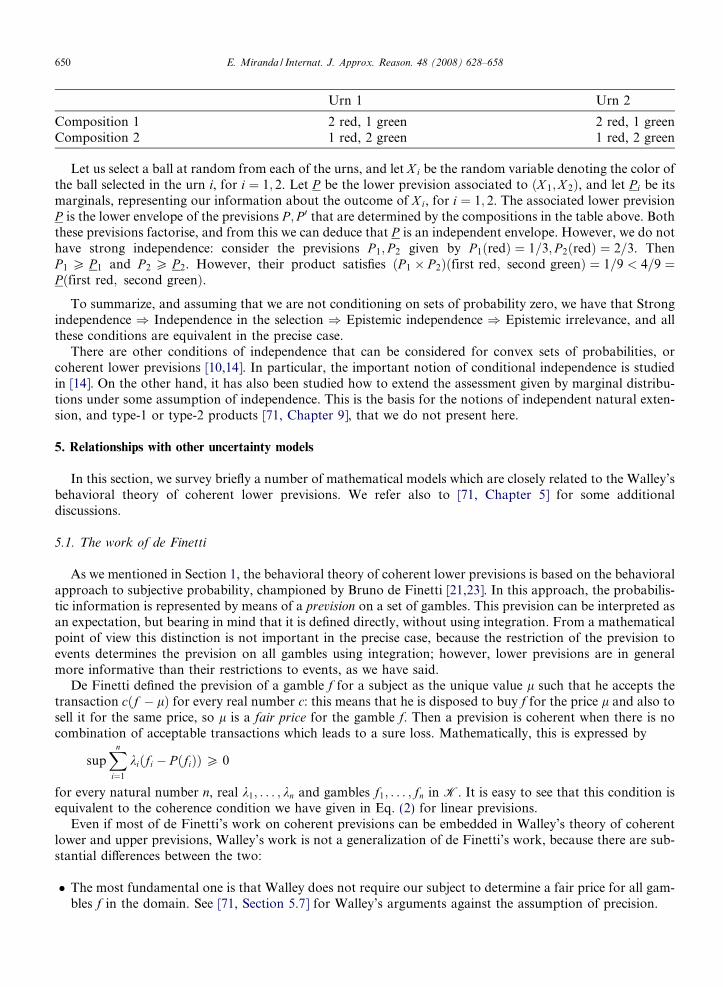
Urn 1 Urn 2

Composition 1 2 red, 1 green 2 red, 1 greenComposition 2 1 red, 2 green 1 red, 2 green


Let us select a ball at random from each of the urns, and let X i be the random variable denoting the color ofthe ball selected in the urn i, for i ¼ 1; 2. Let P be the lower prevision associated to ðX 1;X 2Þ, and let P i be itsmarginals, representing our information about the outcome of X i, for i ¼ 1; 2. The associated lower previsionP is the lower envelope of the previsions P ; P 0 that are determined by the compositions in the table above. Boththese previsions factorise, and from this we can deduce that P is an independent envelope. However, we do nothave strong independence: consider the previsions P 1; P 2 given by P 1ðredÞ ¼ 1=3; P 2ðredÞ ¼ 2=3. ThenP 1 P P 1 and P 2 P P 2. However, their product satisfies ðP 1 � P 2Þðfirst red; second greenÞ ¼ 1=9 < 4=9 ¼Pðfirst red; second greenÞ.

To summarize, and assuming that we are not conditioning on sets of probability zero, we have that Strongindependence ) Independence in the selection ) Epistemic independence ) Epistemic irrelevance, and allthese conditions are equivalent in the precise case.

There are other conditions of independence that can be considered for convex sets of probabilities, orcoherent lower previsions [10,14]. In particular, the important notion of conditional independence is studiedin [14]. On the other hand, it has also been studied how to extend the assessment given by marginal distribu-tions under some assumption of independence. This is the basis for the notions of independent natural exten-sion, and type-1 or type-2 products [71, Chapter 9], that we do not present here.

5. Relationships with other uncertainty models

In this section, we survey briefly a number of mathematical models which are closely related to the Walley’sbehavioral theory of coherent lower previsions. We refer also to [71, Chapter 5] for some additionaldiscussions.

5.1. The work of de Finetti

As we mentioned in Section 1, the behavioral theory of coherent lower previsions is based on the behavioralapproach to subjective probability, championed by Bruno de Finetti [21,23]. In this approach, the probabilis-tic information is represented by means of a prevision on a set of gambles. This prevision can be interpreted asan expectation, but bearing in mind that it is defined directly, without using integration. From a mathematicalpoint of view this distinction is not important in the precise case, because the restriction of the prevision toevents determines the prevision on all gambles using integration; however, lower previsions are in generalmore informative than their restrictions to events, as we have said.

De Finetti defined the prevision of a gamble f for a subject as the unique value l such that he accepts thetransaction cðf � lÞ for every real number c: this means that he is disposed to buy f for the price l and also tosell it for the same price, so l is a fair price for the gamble f. Then a prevision is coherent when there is nocombination of acceptable transactions which leads to a sure loss. Mathematically, this is expressed by

supXn

i¼1

kiðfi � P ðfiÞÞP 0

for every natural number n, real k1; . . . ; kn and gambles f1; . . . ; fn in K. It is easy to see that this condition isequivalent to the coherence condition we have given in Eq. (2) for linear previsions.

Even if most of de Finetti’s work on coherent previsions can be embedded in Walley’s theory of coherentlower and upper previsions, Walley’s work is not a generalization of de Finetti’s work, because there are sub-stantial differences between the two:

The most fundamental one is that Walley does not require our subject to determine a fair price for all gam-bles f in the domain. See [71, Section 5.7] for Walley’s arguments against the assumption of precision.


Although he did not provide a detailed theory of conditional previsions, his interpretation for them isslightly different from Walley’s: he regards them as previsions defined on a family of conditional eventsEjH , where EjH is a logical entity which is true if both E and H are true, false if H is true and E is false,and void if H is false. Another difference between the two approaches is their regard towards the condition of conglomerability,

which is rejected by de Finetti in [23, Section 4.19]: he gives two examples where conglomerability is notsatisfied. One argument here is that full conglomerability rules out linear previsions which are not count-ably additive (see Section 3.3 for a more precise formulation). The key of the matter, as Walley says in [71,p. 327] is that

8 Thsupx2su

really

‘‘Those who insist on additivity and linearity must either reject conglomerability or the possibility ofextensions to larger domains.”

5.2. The work of Williams

A first approach to generalizing de Finetti’s work taking into account the presence of imprecision was con-sidered by Peter Williams in [84–86] (see also [67] for a recent review of Williams’ work). It was also motivatedby the treatment of conditional previsions in de Finetti’s work. Williams defines a coherent conditional lowerprevision by means of a set of acceptable gambles, in the sense that P ðf jBÞ is defined as the supremum value ofl such that IBðf � lÞ is an acceptable transaction for our subject. In particular, if we consider B ¼ X; P ðf jXÞagrees with Walley’s behavioral interpretation of a lower prevision (see [86] for a more detailed account of theunconditional case). Similarly, P ðf jBÞ is defined as the infimum value of l such that the gamble IBðl� f Þ isacceptable for our subject, which in the case of unconditional lower previsions ðB ¼ XÞ becomes the infimumselling price for f.

In order to define coherence, he requires the set of acceptable gambles to satisfy conditions which areslightly weaker than (D0)–(D3).8 He proves then that a necessary condition for coherence is that

supx2[n

i¼0Bi

Xn

i¼1

kiIBiðfi � P ðfijBiÞÞ � k0IB0ðf0 � P ðf0jB0ÞÞ

" #ðxÞP 0 ð13Þ

for every natural number n, Bi included in X, non-negative real ki and fi in the domain of P ð�jBiÞ fori ¼ 0; . . . ; n. This condition is sufficient if we require the set of acceptable gambles to satisfy (D0)–(D3).

Let us compare this Condition, that we shall call W-coherence, with Walley’s notion of coherence for con-ditional lower previsions (11). We see that, under Walley’s terminology (see Section 3.2), Condition (13)corresponds to the particular case of Eq. (11) where the sets SiðfiÞ are finite for all i. Hence, if we considera number of conditional lower previsions P ð�jB1Þ; . . . ; Pð�jBnÞ where B1; . . . ;Bn are finite partitions of X, thenthey are coherent in the sense of Walley if and only if they are W-coherent. However, for arbitrary (not nec-essarily finite) partitions B1; . . . ;Bn, Walley’s notion of coherence is stronger than that of Williams.

The use of W-coherence for conditional lower previsions has a number of technical advantages over Wal-ley’s condition:

W-coherent conditional lower previsions are always lower envelopes of sets of W-coherent conditional lin-ear previsions ([85, Theorem 2], see also [71, Section 8.1]), and as a consequence they can be given a Bayes-ian sensitivity analysis interpretation. We can always construct the smallest W-coherent extension of a W-coherent conditional lower prevision

[85, Theorem 1]. Moreover, this result can be generalized towards unbounded gambles [63].

e difference is that he does not require a gamble f 6¼ 0 with infx2suppðf Þf ðxÞ ¼ 0 to be accepted, nor a gamble f 6¼ 0 with

ppðf ÞðxÞ ¼ 0 to be rejected, where suppðf Þ ¼ fx 2 X : f ðxÞ 6¼ 0g is the support of f. This is related also to Walley’s discussion ofdesirable gambles [71, Appendix F].


There are also, however, a number of drawbacks:

If we express the condition using Walley’s terminology, it assumes the finiteness of the sets SiðfiÞ involved,whereas for many statistical applications it is important to consider non-finite spaces and partitions. It does not satisfy in general the conglomerability condition, as a consequence when we consider infinite par-

titions we may end up with acceptable transactions (W-coherent) which incur in a sure loss [71, Example 6.6.9].

As a summary, Williams’ definition of coherence is a valid and interesting alternative to Walley, that avoidssome of the drawbacks of Walley’s approach to conditional lower previsions. Moreover, it seems to be bettersuited for extending the theory to unbounded gambles. The choice between the two is based in whether weaccept full conglomerability as a rationality requirement, which means essentially that we assume countableadditivity of the involved previsions (but without measurability requirements): see Section 3.3 and [71, Section6.9] for more details.

5.3. Kuznetsov’s work on interval-valued probabilities

In a relatively unknown book on interval-valued probabilities [40], the Russian mathematician V. Kuznetsovestablished, in parallel to Walley, a theory of interval-valued probabilities and previsions which has many thingsin common with the behavioral theory we have presented. Starting from some axioms which are equivalent toWalley, he deduces many of the properties that can also be found in Walley’s book. He also obtains some inter-esting limit results for coherent lower and upper previsions. The main differences between both theories are:

Kuznetsov does not consider the behavioral interpretation for coherent lower and upper previsions in termsof buying and selling prices. He makes some assumptions in the domains, and therefore we cannot consider previsions with arbitrary

domains as is the case with Walley’s theory. His theory is valid for unbounded gambles, and the domain of his upper previsions contains at least those

gambles which are bounded above (and similarly, the domain of his lower previsions includes at least thegambles which are bounded below). When conditioning on a set B of lower probability zero and positive upper probability, he suggests taking

the limit on conditional dominating previsions, which give positive probability to B. This is related to thenotion of regular extension in Walley [71, Appendix K].

See [41,42] for two short papers in English presenting Kuznetsov’s work, and [12,66] for some worksderived from his theory.

5.4. Weischelberger’s F- and R-probabilities

Recently, Kurt Weischleberger and some of his colleagues have also established a theory of interval-valuedprobabilities [79–81] that is more statistically oriented than Walley’s. This theory considers two non-additivemeasures L 6 U determining the lower and upper bounds for our probabilities. The set of (finitely additive)probabilities M that lie between L and U are called the structure determined by L;U .

L and U are said to determine an R-probability with structure M when M 6¼ ;, and an F-probability whenL;U are the infimum and the supremum of the probabilities in M, respectively. Hence, these concepts areequivalent to the notions of avoiding sure loss and coherence for imprecise probabilities.

Weischleberger’s theory is more related to the classical works on probability theory, in the sense that itfocuses on probabilities instead of previsions and that it also makes some measurability assumptions thatare not present in Walley’s theory. Another difference is that Weischelberger’s work does not use a subjectiveinterpretation of lower and upper probabilities, and it allows to connect the notions of avoiding sure loss andcoherence with a frequentist interpretation of probability (see also [69] for another paper in this direction). Thetreatment of conditional lower and upper probabilities and of the notion of independence is also different [82].

See [2,82] for some recent work based on this theory.


5.5. The Dempster–Shafer theory of evidence

Next, we outline the main features of the Dempster–Shafer theory of evidence [57]. The origin of this theoryis in Dempster’s work on random sets, or measurable multi-valued mappings [24,25].

Let A be a field of subsets of X, and consider a lower probability P : A! ½0; 1� that satisfiesP ð;Þ ¼ 0; P ðXÞ ¼ 1. P is said to be completely monotone if it is monotone and for any events A1; . . . ;An inA and n P 2,

P ð[ni¼1AiÞP

XI�f1;...;ng

ð�1ÞjI jþ1P ð\i2I AiÞ; ð14Þ

where jI j denotes the cardinality of the set I. A lower probability that satisfies Eq. (14) for all k 6 p is called p-monotone. A complete monotone lower probability is then one that is n-monotone for every natural numbern. When X is a finite space, and the field A is the class of all subsets of X, a completely monotone lower prob-ability is called a belief function. A belief function is determined by its so-called basic probability assignment m,which is given by

mðAÞ ¼XB�A

ð�1ÞjA�BjP ðBÞ:

Then P is given, for all A � X , by PðAÞ ¼P

B�AmðBÞ. The upper probability that we can generate from a com-pletely monotone lower probability using conjugacy is said to be completely alternating, and, in the particularcase where X is finite, a plausibility function. The relationship between a plausibility function P and the basicprobability assignment m of its conjugate belief function P is P ðAÞ ¼

PB\A 6¼;mðBÞ. The basic probability

assignment of a set A can be interpreted as the measure of belief that is committed exactly to A. ThenP ðAÞ would be our subject’s belief that the result of the experiment belongs to the set A, while P ðAÞ is the mea-sure of his belief that the outcome of the experiment may belong to A (or, perhaps more clearly, the measure ofbelief that does not rule out that the outcome is in A). This is the so-called evidential interpretation.

From the behavioral point of view, multi-valued mappings have been studied in [71, Section 4.3.5] and in [47].On the other hand, 2- (and in particular completely-) monotone functions were studied by Walley in [68]. Some ofhis results generalize to the case where the domain is a lattice of events instead of a field [18]. It can be checked [68]that a 2-monotone lower probability is in particular coherent, and therefore so are n- and completely monotonecapacities. More generally, we can consider n-monotone lower previsions, which appeared in [5, Chapter 3] asfunctionals between an Abelian semigroup and an Abelian group, and were studied from a behavioral pointof view in [17,18]. Hence, from a static point of view (without considering updating or combination of informa-tion) Dempster–Shafer theory can be embedded into Walley’s theory of coherent lower previsions.

One of the main features of the evidential theory, and Walley’s main point of criticism (see [71, Section 5.13]and [74]) is Dempster’s Rule of Combination [24,57]. It is used to combine several belief functions which arebased on different sources of information into one belief function. Let P 1; P 2 be two belief functions with basicprobability assignments m1;m2, respectively. The combined belief function P is the one related to the basicprobability assignment

mðCÞ ¼X

A\B¼C

m1ðAÞm2ðBÞ; ð15Þ

where, if necessary, we normalize it by multiplying by

1�X

A\B¼;m1ðAÞm2ðBÞ

" #�1

;

which is a measure of the extent of the conflict between P 1 and P 2.This rule of combination is only reasonable for Walley provided we make some additional assumptions on

the relationship between the experiments that underlie P 1; P 2 [71, Section 5.13.7]. In particular, the condition-ing rule that we may derive from it may fail to produce conditional lower previsions which are coherent withthe unconditional ones. We may have to make some extra assumptions of conditional independence if we want


it to satisfy coherence, and this requirement may be unreasonable in some cases. See also [44,50,87] for furthercriticism of this rule.

5.6. The game-theoretic approach to imprecise probabilities

We would like to conclude this section by making a brief summary of recent work by Shafer and Vovk [59],where a connection is established between probability and finance through a game-theoretic approach tocoherent lower previsions. The ideas of this approach are roughly similar to the ones behind the behavioraltheory we have outlined: we also have here acceptable transactions and study whether they can lead to a sureloss. There are, however, a number of important differences between the two: Shafer and Vovk consider agame between two players, whereas Walley’s theory is focused on one subject who establishes buying and sell-ing prices;9 there is no assumption of boundedness of the variables involved; and they focus on the conse-quences and not so much on probability.

Let us make a short summary of the main ideas in this work. We refer to [59,60] for more details. Considera game between two players, called World and Skeptic, who play according to a certain protocol. The firstplayer (World) can make a number of moves, where the next move may depend on his previous moves,but not on the ones made by Skeptic. These moves can be represented in a tree, and we call a situation someconnected path in the tree that starts at the root of the tree.

In each situation t, Skeptic has a number of possible moves, and a gain function associated to the move hemakes and World’s next move, representing the change in Skeptic capital associated to these two moves. Astrategy is then a function determining Skeptic next move for each non-final situation in the tree representingWorld’s moves, and the associated capital if he starts the game with zero capital is his capital process.

Under this interpretation, Shafer and Vovk define upper and lower prices for real variables. The upper price

for a variable f in a non-final situation t is the lowest price at which Skeptic can buy the variable f at the end ofthe game, no matter what moves World makes, using some strategy. The lower price for a variable f in a non-final situation t can be given an analogous interpretation using conjugacy.

A gambling protocol is called a probability protocol when the following two conditions are satisfied:

(PP1) The set of possible moves for Skeptic in any situation t is a convex cone.(PP2) For each non-final situation, Skeptic’s gain function is linear with respect to Skeptic’s moves, for any

move of World fixed.

It is called coherent when for each non-final situation and each possible move s of Skeptic there is anothermove w of World such that the gain associated to ðs;wÞ is non-positive.

For many of their developments Shafer and Vovk decompose World into multiple players. They consider forinstance Reality and Forecaster, where Forecaster determines for each non-final situation the set of possiblemoves and the gain function for Skeptic, while Reality determines the move of World. Shafer and Vovk establisha number of limit results, such as weak and strong laws of large numbers, for coherent probability protocols.

Under the terminology we have considered throughout this survey, our subject would take the role of Fore-caster, in the sense that he establishes the supremum buying prices for all gambles in the domain. Then, wecheck the coherence of these prices using the roles of Skeptic (selecting some gambles in the domain) and Real-ity (determining the outcome of the experiment, that is, the value x in X). Walley’s notion of coherence meansthat the buying prices established by Forecaster should not be exploitable by Skeptic in order to assure himselfa gain, no matter how World moves.

We see then that, although some of the concepts used by Shafer and Vovk are similar to the ones in Wal-ley’s theory of coherent lower previsions (the behavioral interpretation, the notion of coherence, etc.), thereare also differences between the two approaches, like the use of two players and the extension to unboundedgambles. It is therefore interesting that Shafer and Vovk’s work on coherent probability protocols has beenrecently connected to Walley’s theory of coherent lower previsions in [19]. It has been proven that for every

9 A two player model is already present in [61].


coherent probability protocol there exists an immediate prediction model such that both lead to identical buy-ing prices, and vice versa. See [19] for more information. In this sense, in spite of some of their differences, theresults from one theory can be embedded into the other.10

6. Applications

Let us give some comments now on the use of the theory of coherent lower previsions in other contexts.Since the origins of subjective probability are in decision making, it is not really surprising that much ofthe work made on practical uses of coherent lower previsions, which stem from subjective probability theory,is related to decision theory. Indeed, imprecise probabilities can be seen as a more realistic model for practicaldecision problems, because they allow us to treat some of the most common problems that appear in practice:lack of available information, conflicting sources of beliefs, and difficulties in eliciting expert’s opinions.

The theory of coherent lower previsions, in different forms, has been employed in a number of applications,in different frameworks such as the environmental [70] or the bio-medical [64,72,90]. One of the consequencesof the use of sets of probabilities will be that sometimes we cannot decide which of two alternatives must bepreferred, something which is to be expected on the other hand in the case of little information. Another fea-ture is that there are many possible ways of generalizing the principle of maximum expected utility to coherentlower previsions, such as E-admissibility, interval dominance, C-maximinity and maximality, etc. We refer to[65] for an overview of the different criteria, and to [56] for a comparison of E-admissibility and C-maximinity.There have also been several studies connecting the behavioral theory of coherent lower previsions with dif-ferent aspects of statistics [73,75]. One of the most important is the work in [73], where Walley defined the so-called Imprecise Dirichlet Model. This is a model for inference which relates past and future observationsabout some variables. See also [3,76] for additional information about this model. The Imprecise DirichletModel has been applied in different contexts, such as classification [1,90,91], reliability analysis [9] or gametheory [52]. See also [16,89] for further theoretical developments on this subject.

Finally, coherent lower previsions have also been used for dealing with uncertainty scenarios in climatechange [39] and forestry [28].

7. Strengths and challenges

The results mentioned in this paper constitute an attempt to overview the main features of the behavioraltheory of coherent lower previsions. As a summary, the main virtues of this theory are:

1. It is better suited for situations where the available information does not justify the use of a precise prob-ability distribution.

2. It encompasses most of the other generalizations considered in the literature (belief functions, 2-monotonecapacities, coherent lower probabilities). This is done mainly in two ways: By focusing on the behavior towards variables (gambles), and therefore on the notion of expectation,

without going through the behavior on events first. By moving away from the measurability requirements on classical probability theory and considering

previsions for arbitrary sets of gambles.

3. It provides a behavioral interpretation that leads naturally to decision making, and it can at the same timebe given a sensitivity analysis representation in some cases.

Nevertheless, the theory of coherent lower previsions has a number of challenges that need to be studied inmore detail:

10 The (possible) unboundedness of the variables in the models is overcome in the case of coherent lower previsions by working with setsof (really) desirable gambles, instead of almost-desirable ones [19, Sections 3 and 4].


1. The concept of coherence, although a reasonable rationality requirement, may be too weak to produceinformative inferences.

2. The theory is established for bounded random variables, or gambles, and the generalization towardsunbounded random variables is not straightforward.

3. Like other theories, it assumes the linearity of the utility scale, something which may not be reasonable inpractice.11

4. Walley’s notion of natural extension of conditional lower previsions has some undesirable properties, whichdo not seem to be resolvable without giving up on conglomerability.

5. Computing with coherent lower previsions in practice means often solving non-linear problems, whence forbig problems the computational costs may be high.

6. There have been until now relatively few applications, and more are needed in order to effectively comparethe applicability of this theory with classical tools.

7. More generally, we need to develop tools to be able to compare the effectiveness of precise and impreciseapproaches in a number of situations.

8. There are several notions of independence as well as different optimality criteria, and it is not always clearwhich of them is better suited for each situation.

9. From the theoretical point of view there are a number of notions and results from classical probability the-ory which have not been generalized, such as ergodic theorems.

These problems constitute the main avenues for future research in the theory.

Acknowledgements

I would like to express my gratitude to Gert de Cooman, Marco Zaffalon, Roman Effremov and the anon-ymous referees for some very helpful comments that improved substantially earlier versions of this paper. Ialso acknowledge the financial support of the project TSI2007-66706-C04-01.

References

[1] A. Antonucci, A. Salvetti, M. Zaffalon, Credal networks for hazard assessment of debris flows, in: J. Kropp, J. Scheffran (Eds.),Advanced Methods for Decision Making and Risk Management in Sustainability Science, Nova Science, 2007, pp. 237–256.

[2] T. Augustin, F. Coolen, Non parametric predictive inference and interval probability, Journal of Statistical Planning and Inference124 (2004) 251–272.

[3] J.M. Bernard, An introduction to the imprecise Dirichlet model for inference with multinomial data, International Journal ofApproximate Reasoning 39 (2–3) (2005) 123–150.

[4] E. Borel, Probabilities and Life, Dover, New York, 1962.[5] G. Choquet, Theory of capacities, Annales de l’Institut Fourier. Universite de Grenoble 5 (1953) 131–295.[6] G. Coletti, Coherent numerical and ordinal probability assessments, IEEE Transactions on Systems, Man and Cybernetics 24 (1994)

1747–1754.[7] G. Coletti, R. Scozzafava, Zero probabilities in stochastic independence, in: R.R. Yager, B. Bouchon-Meunier, L.A. Zadeh (Eds.),

Information, Uncertainty, Fusion, Kluwer, 2000, pp. 185–196.[8] G. Coletti, R. Scozzafava, Probabilistic Logic in a Coherent Setting, Kluwer, New York, 2002.[9] F. Coolen, An imprecise Dirichlet model for Bayesian analysis of failure data including right-censored observations, Reliability

Engineering and System Safety 56 (1997) 61–68.[10] I. Couso, S. Moral, P. Walley, A survey of concepts of independence for imprecise probabilities, Risk, Decision and Policy 5 (2) (2000)

165–181.[11] F. Cozman, Irrelevance and independence relations in quasi-Bayesian networks, in: G.F. Coopen, S. Moral (Eds.), Proceedings of the

14th conference on Uncertainty in Artificial Intelligence, 1998, pp. 89–96.[12] F. Cozman, Constructing sets of probability measures through Kuznetsov’s independence condition, in: Proceedings of the 2nd

International Symposium on Imprecise Probabilities and Their Applications, 2001, pp. 104–111.[13] F. Cozman, P. Walley, Graphoid properties of epistemic irrelevance and independence, Annals of Mathematics and Artificial

Intelligence 45 (1–2) (2005) 173–195.

11 But see [51] for an interesting solution to this problem.


[14] L.M. de Campos, S. Moral, Independence concepts for convex sets of probabilities, in: Proceedings of 11th Conference onUncertainty in Artificial Intelligence, 1995, pp. 108–115.

[15] G. de Cooman, Possibility theory I–III, International Journal of General Systems 25 (4) (1997) 291–371.[16] G. de Cooman, M. Zaffalon, Updating beliefs with incomplete observations, Artificial Intelligence 159 (1–2) (2004) 75–125.[17] G. de Cooman, M.C.M. Troffaes, E. Miranda, n-Monotone lower previsions and lower integrals, in: Proceedings of the 4th

International Symposium on Imprecise Probabilities and Their Applications, 2005, pp. 145–154.[18] G. de Cooman, M.C.M. Troffaes, E. Miranda, n-Monotone lower previsions, Journal of Intelligent and Fuzzy Systems 16 (4) (2005)

253–263.[19] G. de Cooman, F. Hermans, On coherent immediate prediction: connecting two theories of imprecise probability, in: Proceedings of

the 5th International Symposium on Imprecise Probabilities and Their Applications, 2007, pp. 97–106.[20] G. de Cooman, E. Miranda, Symmetry of models versus models of symmetry, in: W.L. Harper, G.R. Wheeler (Eds.), Probability and

Inference: Essays in Honor of Henry E. Kyburg, Jr., King’s College Publications, 2007, pp. 67–149.[21] B. de Finetti, La prevision: ses lois logiques, ses sources subjectives, Annales de l’Institut Henri Poincare 7 (1937) 1–68.[22] B. de Finetti, Teoria delle Probabilita, Einaudi, Turin, 1970.[23] B. de Finetti, Theory of Probability, John Wiley and Sons, Chichester, 1974 (English translation of [22]).[24] A.P. Dempster, Upper and lower probabilities induced by a multivalued mapping, Annals of Mathematical Statistics 38 (1967) 325–

339.[25] A.P. Dempster, Upper and lower probabilities generated by a random closed interval, Annals of Mathematical Statistics 39 (1968)

957–966.[26] D. Denneberg, Non-additive Measure and Integral, Kluwer Academic Publishers, Dordrecht, 1994.[27] D. Dubois, H. Prade, Possibility Theory, Plenum Press, New York, 1988.[28] M. Ducey, Imprecision in a timber asset sale model: motivation, specification, and behavioural implications, in: Proceedings of 2nd

International Symposium on Imprecise Probabilities and Their Applications, 2001, pp. 162–170.[29] S. Ferson, V. Kreinovich, L. Ginzburg, D. Myers, Kari Sentz, Constructing probability boxes and Dempster–Shafer structures,

Technical Report SAND2002–4015, Sandia National Laboratories, January 2003.[30] T. Fine, Theories of Probability, Academic Press, New York, 1973.[31] I.J. Good, Subjective probability as the measure of a non-measurable set, in: E. Nagel, P. Suppes, A. Tarski (Eds.), Logic,

Methodology and Philosophy of Science, Stanford University Press, Stanford, 1962, pp. 319–329.[32] M. Grabisch, H.T. Nguyen, E.A. Walker, Fundamentals of Uncertainty Calculi with Applications to Fuzzy Inference, Kluwer

Academic Publishers, Dordrecht, 1995.[33] J.M. Keynes, A Treatise on Probability, McMillan, London, 1921.[34] F.H. Knight, Risk, Uncertainty and Profit, University of Chicago Press, 1971 (First published in 1921).[35] B. Koopman, The axioms and algebra of intuitive probability, Annals of Mathematics 41 (1940) 269–292.[36] B. Koopman, The bases of probability, Bulletin of the American Mathematical Society 46 (1940) 763–774.[37] B. Koopman, Intuitive probabilities and sequences, Annals of Mathematics 42 (1941) 169–187.[38] P.H. Krauss, Representation of conditional probability measures on Boolean algebras, Acta Mathematica Academiae Scientiarum

Hungaricae 19 (1968) 229–241.[39] E. Kriegler, Utilizing belief functions for the estimation of future climate change, International Journal of Approximate Reasoning 39

(2–3) (2005) 185–209.[40] V. Kuznetsov, Interval statistical models, radio and communication, 1991 (in Russian).[41] V. Kuznetsov, Interval methods for processing statistical characteristics, Reliable Computing, supplement on Extended Abstracts of

APIC’95, 1995, pp. 116–122.[42] V. Kuznetsov, Auxiliary problems of statistical data processing: interval approach, Reliable Computing, supplement on Extended

Abstracts of APIC’95, 1995, pp. 123–129.[43] H.E. Kyburg, H.E. Smokler, Studies in Subjective Probability, Wiley, New York, 1964.[44] H.E. Kyburg, Bayesian and non-Bayesian evidential updating, Artificial Intelligence Journal 31 (1987) 271–294.[45] I. Levi, The Enterprise of Knowledge, MIT Press, Cambridge, 1980.[46] E. Miranda, G. de Cooman, Coherence and independence on non-linear spaces. Technical Reports on Statistics and Decision

Sciences, TR05/10, May 2005. <http://www.deio.urjc.es/publicaciones.php>.[47] E. Miranda, G. de Cooman, I. Couso, Lower previsions induced by multi-valued mappings, Journal of Statistical Planning and

Inference 133 (2005) 173–197.[48] E. Miranda, G. de Cooman, Marginal extension in the theory of coherent lower previsions, International Journal of Approximate

Reasoning 46 (1) (2007) 188–225.[49] S. Moral, Epistemic irrelevance on sets of desirable gambles, Annals of Mathematics and Artificial Intelligence 45 (1–2) (2005) 197–

214.[50] J. Pearl, Reasoning with belief functions: an analysis of compatibility, International Journal of Approximate Reasoning 4 (1990) 363–

390.[51] R. Pelessoni, P. Vicig, Uncertainty modelling and conditioning with convex imprecise previsions, International Journal of

Approximate Reasoning 39 (2–3) (2005) 297–319.[52] E. Quaeghebeur, G. de Cooman, Game theoretic learning using the imprecise Dirichlet model, in: Proceedings of the 3rd International

Symposium on Imprecise Probabilities and Their Applications, 2003, pp. 452–466.[53] D. Rıos Insua, F. Ruggieri, Robust Bayesian Analysis, Springer, 2000.

http://www.deio.urjc.es/publicaciones.php


[54] T. Seidenfeld, L. Wasserman, Dilation for sets of probabilities, Annals of Statistics 21 (3) (1993) 1139–1154.[55] T. Seidenfeld, M. Schervisch, J. Kadane, A representation of partially ordered preferences, Annals of Statistics 23 (6) (1995) 2168–

2217.[56] T. Seidenfeld, A contrast between two decision rules for use with (convex) sets of probabilities: gamma-maximin versus E-admisibility,

Synthese 140 (1–2) (2004) 69–88.[57] G. Shafer, A Mathematical Theory of Evidence, Princeton University Press, New Jersey, 1976.[58] G. Shafer, Non-additive probabilities in the work of Bernoulli and Lambert, Archive for History of Exact Sciences 19 (4) (1978) 309–

370.[59] G. Shafer, V. Vovk, Probability and Finance: It’s Only a Game! John Wiley and Sons, New York, 2001.[60] G. Shafer, P. Gillett, R. Scherl, A new understanding of subjective probability and its generalization to lower and upper prevision,

International Journal of Approximate Reasoning 33 (2003) 1–49.[61] C.A.B. Smith, Consistency in statistical inference and decision (with discussion), Journal of the Royal Statistical Society 23 (1961) 1–

37.[62] M. Troffaes, G. de Cooman, Extensions of coherent lower previsions to unbounded random variables, in: B. Bouchon-Meunier, L.

Foulloy, R. Yager (Eds.), Intelligent Systems for Information Processing: from Representation to Applications, North-Holland,Amsterdam, 2003, pp. 277–288.

[63] M. Troffaes, Conditional lower previsions for unbounded random quantities, in: J. Lawry, E. Miranda, A. Bugarin, S. Li, M.A. Gil,P. Grzegiorzewski, O. Hryniewicz (Eds.), Soft Methods in Integrated Uncertainty Modelling, Springer, 2006, pp. 201–210.

[64] M. Troffaes, Efficient and robust global amino acid sequence alignment with uncertain evolutionary distances, in: B. Bouchon-Meunier, G. Coletti, R. Yager (Eds.), Modern Information Processing: from Theory to Applications, Elsevier, 2006, pp. 371–381.

[65] M. Troffaes, Decision making under uncertainty using imprecise probabilities, International Journal of Approximate Reasoning 45(1) (2007) 17–29.

[66] L. Utkin, I. Kozine, Different faces of the natural extension, in: Proceedings of the 2nd International Symposium on ImpreciseProbabilities and Their Applications, 2001, pp. 316–323.

[67] P. Vicig, M. Zaffalon, F. Cozman, Notes on ‘Notes on conditional previsions’, International Journal of Approximate Reasoning 44(3) (2007) 358–365.

[68] P. Walley, Coherent lower (and upper) probabilities. Statistics Research Report, University of Warwick (Coventry), 22, 1981.[69] P. Walley, T. Fine, Towards a frequentist theory of upper and lower probability, Annals of Statistics 10 (1982) 741–761.[70] P. Walley, F. Campello de Souza, Uncertainty and indeterminacy in assessing the economic viability of energy options: a case study of

solar heating systems in Brazil, Energy, Systems and Policy 14 (1990) 281–304.[71] P. Walley, Statistical Reasoning with Imprecise Probabilities, Chapman and Hall, London, 1991.[72] P. Walley, L. Gurrin, P. Burton, Analysis of clinical data using imprecise prior probabilities, The Statistician 45 (1996) 457–485.[73] P. Walley, Inferences from multinomial data: learning about a bag of marbels, Journal of the Royal Statistical Society, B 58 (1996) 3–

57.[74] P. Walley, Measures of uncertainty in expert systems, Artificial Intelligence 83 (1996) 1–58.[75] P. Walley, A bounded derivative model for prior ignorance about a real-valued parameter, Scandinavian Journal of Statistics 24

(1997) 463–483.[76] P. Walley, J.M. Bernard, Imprecise probabilistic prediction for categorical data, Technical Report CAF9901, Universite Paris 8, 1999.[77] P. Walley, Towards a unified theory of imprecise probability, International Journal of Approximate Reasoning 24 (2000) 125–148.[78] P. Walley, R. Pelessoni, P. Vicig, Direct algorithms for checking consistency and making inferences from conditional probability

assessments, Journal of Statistical Planning and Inference 126 (2004) 119–151.[79] K. Weischelberger, Axiomatic foundations of the theory of interval probability, in: Proceedings of the 2nd Gauss Symposium, 1995,

pp. 47–64.[80] K. Weischelberger, The theory of interval probability as a unifying model for uncertainty, International Journal of Approximate

Reasoning 24 (2000) 149–170.[81] K. Weichselberger, Elementare Grundbegriffe einer allgemeineren Wahrscheinlichkeitsrechnung I: Intervallwahrscheinlichkeit als

umfassendes Konzept (in cooperation with T. Augustin and A. Wallner), Physica, Heidelberg, 2001.[82] K. Weischleberger, The logical concept of probability: foundation and interpretation, in: Proceedings of the 5th International

Symposium on Imprecise Probabilities and Their Applications, 2007, pp. 455–464.[83] P. Whittle, Probability via Expectation, fourth ed., Springer, 2000.[84] P. Williams, Coherence, strict coherence and zero probabilities, in: Proceedings of the Fifth International Congress on Logic,

Methodology and Philosophy of Science, 1975, pp. 29–33.[85] P. Williams. Notes on conditional previsions. Technical report, University of Sussex, 1975. Reprinted in a revised form in the

International Journal of Approximate Reasoning 44(3) (2007) 366–383.[86] P. Williams, Indeterminate probabilities, in: M. Przelecki, K. Szaniawski, R. Wojcicki (Eds.), Formal Methods in the Methodology

of Empirical Sciences, D. Reidel Publishing Company, 1976, pp. 229–246.[87] P. Williams, On a new theory of epistemic probability, British Journal for the Philosophy of Science 29 (4) (1978) 375–378.[88] L.A. Zadeh, Fuzzy sets as a basis for a theory of possibility, Fuzzy Sets and Systems 1 (1) (1978) 3–28.[89] M. Zaffalon, Exact credal treatment of missing data, Journal of Statistical Planning and Inference 105 (1) (2002) 105–122.[90] M. Zaffalon, K. Wesnes, O. Petrini, Reliable diagnoses of dementia by the naive credal classifier from incomplete cognitive data,

Artificial Intelligence in Medicine 29 (1–2) (2003) 61–79.[91] M. Zaffalon, Credible classification for environmental problems, Environmental modelling and software 20 (8) (2005) 1003–1012.

Documents

A survey of the theory of coherent lower previsions