A Theory of Binary Digital Pictures - Department of … THEORY OF BINARY DIGITAL PICTURES 223 is simply-connected if given any two curves in Y with the same endpoints we can transform

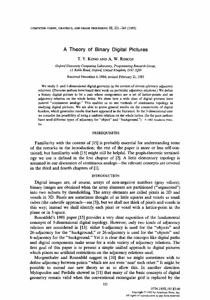
COMPUTER VISION, GRAPHICS, AND IMAGE PROCESSING 32, 221-243 (1985)

A Theory of Binary Digital Pictures

T. Y. KONG AND A. W. ROSCOE

Oxford University Computing Laboratory, Programming Research Group, 11 Keble Roa~ Oxford, United Kingdom, OXI 3QD

Received December 4, 1984; revised February 21, 1985

We study 2- and 3-dimensional digital geometry in the context of almost arbitrary adjacency relations. (Previous authors have based their work on particular adjacency relations.) We define a binary digital picture to be a pair whose components are a set of lattice-points and an adjacency relation on the whole lattice. We show how a wide class of digital pictures have natural "continuous analogs." This enables us to use methods of continuous topology in studying digital pictures. We are able to prove general results on the connectivity of digital borders, which generalize results that have appeared in the literature. In the 3-dimensional case we consider the possibility of using a uniform relation on the whole lattice. (In the past authors have used different types of adjacency for "object" and "background.") �9 1985 Academic Press, Inc.

PREREQUISITES

Familiarity with the content of [15] is probably essential for understanding some of the remarks in the introduction; the rest of the paper is more or less self-contained, but familiarity with [15] might still be helpful. The graph-theoretic terminology we use is defined in the first chapter of [3]. A httle elementary topology is assumed in our discussion of continuous analogs--the relevant concepts are covered in the third and fourth chapters of [1].

INTRODUCTION

Digital images are, of course, arrays of non-negative numbers (gray values); binary images are obtained when the array elements are partitioned ("segmented") into two subsets by thresholding. The array elements are called pixels in 2D and voxels in 3D. Pixels are sometimes thought of as little squares and voxels as small cubes (the cuberille approach--see [5]), but we shall not think of pixels and voxels in this way; instead we shall identify each pixel or voxel with a lattice-point in the plane or in 3-space.

Rosenfeld's 1981 paper [15] provides a very clear exposition of the fundamental concepts of 3-dimensional digital topology. However, only two kinds of adjacency relation are considered in [15]: either 6-adjacency is used for the "objects" and 26-adjacency for the "background," or 26-adjacency is used for the "objects" and 6-adjacency for the "background." Yet it is clear that the concepts like digital paths and digital components make sense for a wide variety of adjacency relations. The first goal of this paper is to present a simple unified approach to digital pictures which places no artificial restrictions on the adjacency relations used.

Morgenthaler and Rosenfeld suggest in [10] that we might sometimes wish to define adjacency between points "which are not even 'near' each other." It might be possible to extend our new theory so as to allow this. In another direction Mylopoulos and Pavlidis showed in [11] that many of the basic concepts of digital geometry remain valid when the conventional rectangular grid is replaced by the

221 0734-189X/85 $3.00

Copyright �9 1985 by Academic Press, Inc. All rights of reproduction in any form reserved.

222 KONG AND ROSCOE

Cayley diagram (of. [3, Chap. 8]) of any finite presentation of an abelian group--they called such group presentations discrete spaces. It is likely that the ideas introduced in our present article can be applied to many of these discrete spaces.

Further motivation for the present paper comes from our investigation of the "surface-points" introduced by Morgenthaler, Reed, and Rosenfeld [10, 13, 12]. In our paper [7] we prove non-trivial results by transforming problems of digital topology into problems of polyhedral topology. The transformation is done by constructing "continuous analogs" of digital pictures. However, the full potential of this approach is not realized in [7]: although continuous analogs exist for "most" digital pictures, their existence is proved only in very special cases. The second goal of this paper is to develop a general theory of continuous analogs and to give good necessary and sufficient conditions for their existence.

Our work on general binary digital pictures has interesting corollaries for particular adjacency relations. Not only can we obtain Propositions 5 and 6 of [15] but we also find that similar results hold for every pair of "pure" adjacency relations (6-, 18-, or 26-adjacency) other than (6, 6). We regard a proof of these results as our third goal. That these results are fairly deep becomes apparent when we note that the 2-dimensional analogs of both results fail on the surface of a cylinder (when Z 2 is replaced by Z , • Z, where Z n denotes the integers modulo n). The point is that if n is large then Z n • Z is locally indistinguishable from Z 2, which shows that the two propositions express global properties of Euclidean space. (Geometric topol- ogists will recognize that the propositions express discrete versions of two "Phragmen-Brouwer properties" [18]). Many of the propositions proved in our earlier paper [7] are also global results in this sense.

To establish the validity of such results we must use a "global proof method": purely local methods (such as straightforward induction on the number of points in S, or simple graph-theoretic arguments) are unlikely to suffice. Our method of attack involves applying techniques from continuous topology to the continuous analogs of binary digital pictures. We do this in the "IV implies I" part of the proof of Theorem 2.

Finally we point out some of the drawbacks of using any single elementary adjacency relation (4-, 6-, 26-, etc.) on the conventional square and cubic grids. In order to overcome these difficulties many other workers have resorted to the use of different adjacency relations for object and background points. Our investigations suggest that for some purposes it may be a better choice to use a 2-dimensional hexagonal lattice or a 3-dimensional face-centered cubic lattice equipped with the corresponding "nearest neighbor" adjacency relations.

This paper is structured in such a way that it is possible to omit the sections relating to continuous analogs, and the proofs of Theorems 2 and 2', provided that the "I is equivalent to II" part of these theorems is assumed without proof. The statement and proof of Proposition 3 may also be omitted on a first reading; however, the corollary to Proposition 3 is used in the proof of Proposition 4.

SIMPLY-CONNECTED SETS

It will emerge from our paper that Propositions 5 and 6 in [15] are valid because R 2 and R 3 are both simply-connected.

A connected subset Y of R 2 or R 3 is said to be simply-connected if it has no "holes." (A solid cube is simply-connected but a solid torus is not.) Equivalently, Y

A THEORY OF BINARY DIGITAL PICTURES 223

is simply-connected if given any two curves in Y with the same endpoints we can t ransform one curve into the other by means of a "continuous deformation" during which both endpoints remain fixed and the rest of the curve remains in Y. The precise definition is as follows:

A curve in a subset Yof R 1 is a continuous map `/: [0,1] --, Y. The curve ` / is said to be a curve in Y from the point `/(0) to the point ,/(1). The trace of a curve `/ is another name for the image of `/. A connected subset Y of R" is said to be simply-connected if given any two points p and q in Y and any two curves `/0 and /̀1 each of which is a curve in Y from p to q, we can find a continuous map h: [0,1] • [0,1] --, Y such that for all s and t in [0,1] we have

(i) h(s,O)= Vo(S) (ii) h(s, 1) = `/l(s)

(iii) h (0, t) = p

(iv) h (1, t) = q.

The "continuous deformation" h is called a fixed endpoint homotopy of `/0 onto `/1. I t is customary to think of t as "' time."

The definition we have just given is the one we shall use; but it is not the standard definition. We show in the Appendix that the two definitions are equivalent. We asserted above that a solid torus is not simply-connected. This is intuitively clear but not so easy to prove. However, it is a corollary of Theorem 2 below.

ELEMENTARY TERMINOLOGY

In this paper Z denotes the set of integers and R denotes the set of real numbers; Z is regarded as a subset of R. Thus R" denotes Euclidean n-space and Z" is the set of all lattice-points in Euclidean n-space.

Recall that two points in 13 are said to be 26-adjacent if they are distinct and each coordinate of one differs from the corresponding coordinate of the other by at most 1; two points are 18-adjacent if they are 26-adjacent and differ in at most two of their coordinates; two points are 6-adjacent if they are 26-adjacent and differ in at most one coordinate. Two points (x, y ) and (x ' , y ' ) in Z 2 are said to be 8-adjacent or 4-adjacent according as (x, y,O) and (x ' , y',O) are 26-adjacent or 6-adjacent. Unless otherwise stated the greek letters a, p, `/, and 8 will denote integers from the set (4, 8, 6, 18, 26}. We use the term "latt ice-point" to denote a point in Z 2 or Z 3. In this paper we identify Z n with the set of points in R n that have integer coordinates (in the obvious way). If W _c Z" then W c denotes the complementary set Z ' \ W (here n = 3 in the sections relating to 3-dimensional digital pictures and n = 2 in the sections on 2-dimensional pictures). A unit cell is a closed unit cube (in 3D) or a closed unit square (2D) whose corners are all lattice-points. (Note that a unit cell is a connected subset of R 3 or R 2 and not a set of lattice-points.) A window is any union of unit cells.

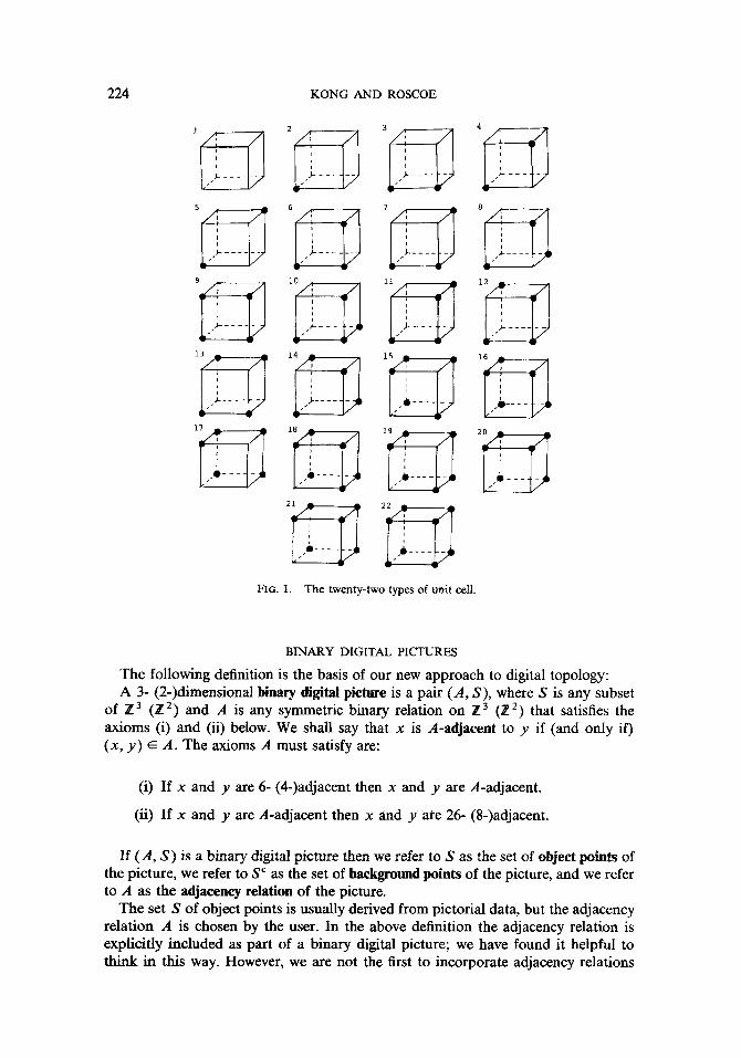
I f K is a unit cell and S _ Z 3 then K N S can be mapped by rotation or reflection onto one of the 22 sets shown in Fig. 1. (A proof is given in the Appendix, but in any event it is readily confirmed that Fig. 1 does exhaust all possibilities.) We shall say that the pair (K, S) is of type n if K (3 S can be mapped by rotation or reflection on the nth set in Fig. 1.

224 KONG AND ROSCOE

v v - - v

FIG. 1. The twenty-two types of unit cell.

BINARY DIGITAL PICTURES

The following definition is the basis of our new approach to digital topology: A 3- (2-)dimensional binary digital picture is a pair (A, S), where S is any subset

of Z 3 (Z 2) and A is any symmetric binary relation on Z 3 (Z 2) that satisfies the axioms (i) and (ii) below. We shall say that x is A-adjacent to y if (and only if) (x, y) ~ A. The axioms A must satisfy are:

(i) If x and y are 6- (4-)adjacent then x and y are A-adjacent.

(ii) If x and y are A-adjacent then x and y ate 26- (8-)adjacent.

I f (A, S) is a binary digital picture then we refer to S as the set of object points of the picture, we refer to S c as the set of background points of the picture, and we refer to A as the adjacency relation of the picture.

The set S of object points is usually derived from pictorial data, but the adjacency relation A is chosen by the user. In the above definition the adjacency relation is explicitly included as part of a binary digital picture; we have found it helpful to think in this way. However, we are not the first to incorporate adjacency relations


into the mathematical structure of a digital picture. Previous authors did so implicitly when using terms like "connectedness in the sense of the background."

Nevertheless, the definition just given represents a slight but significant departure f rom the usual conceptual framework of digital geometry, because the adjacency relation has been freed of all dependence on the set of object points: there is no longer any notion of "adjacency in the S (or S c) sense." In the rest of this paper (A, S) will be a 2- or 3-dimensional binary digital picture.

MORE ELEMENTARY TERMINOLOGY

In this section and the next we adapt the terminology of [15] to our new definition of digital pictures.

If two points are A-adjacent then each is called an A-neighbor of the other. A point is A-adjacent to a set if it is A-adjacent to some member of that set. Two disjoint sets of lattice-points will be said to be A-adjacent if there is a point in one subset that is A-adjacent to some point in the other. An A-path is a sequence of distinct lattice-points such that any two consecutive points in the sequence are A-adjacent. If each point in an A-path belongs to some set T then we shall call the path an A-path in T. An A-path whose first point is x and whose last point is y will be called an A-path from x to y, or alternatively an A-path that links x to y. We shall say S is A-connected if every pair of points in S is linked by an A-path. An A-connected subset of S that is not A-adjacent to any other point in S will be called an A-component of S. Thus S is A-connected iff S contains just one A-component. If S and T are disjoint sets of lattice-points then the (A, S)-border of T (or, alternatively, the A-border of T with respect to S) is defined to be the set of all points in T that are A-adjacent to a point in S.

If A is an adjacency relation on 12 or Z 3 and X is a window then A ( X ) denotes the adjacency relation on the set of lattice-points in X such that x is A(X)-adjacent to y ill' there is a unit cell in X which contains both x and y, and x is A-adjacent to y.

We shall frequently want to use these definitions in the special cases where A is the a-adjacency relation for some a; it will then be very convenient to use the prefix " a " in place of "A." Thus we might refer to an 18-component ( = an A-component where A is the 18-adjacency relation), or " t h e (6, S)-border of T " ( = the (A, S)- border of T where A is the 6-adjacency relation. This use of the numbers 6, 18, 26, 4, and 8 as prefixes is fully consistent with the usage established by previous authors [15,10,13,12], etc.).

If K is any unit cell in R 2 then we define K* to be the union of K with the four other unit cells that have an edge in common with K. Similarly, if K is any unit cell in R 3 then we define K* to be the union of K with the six other unit cells that have a face in common with K.

Finally, we define A(a, ~, "/, S) to be the adjacency relation on Z 2 or Z 3 in which two points x, y are adjacent iff either x and y are a-neighbors in S or x and y are ~8-neighbors in S c or x and y are ,/-neighbors, and exactly one of x and y belongs to S.

ADJACENCY GRAPHS

Let X be any window. The X-adjacency graph of (A, S), denoted by adj(A, X, S), is a (possibly infinite) bipartite graph each of whose vertices is a whole A(X)-com-

226 KONG AND ROSCOE

ponent of S N X or S c n X. The first vertex class of adj(A, X, S) consists of the vertices corresponding to A(X)-components of S O X (these are called the S-vertices of adj(A, X, S)); the second vertex class consists of the vertices corresponding to A(X)-components of S ~ O X (these are called the SC-vertices of adj(A, X, S)). An S-vertex x and an S%vertex y are joined by an edge of adj(A, X, S) if and only if the components represented by x and y are A(X)-adjacent.

The adjaeeney graph of (A, S), which we denote by adj(A, S) is defined to be the (possibly infinite) graph adj(A, R3, S) (3D case) or adj(A, R2, S) (2D case). "adj (a , fl, -/, S )" will be an abbreviation for "adj(A(a, fl, y, S), S)." Thus the S- and SC-vertices of adj(a, fl, 3', S) are respectively the a-components of S and the fl-components of S~; and an S-vertex is joined to an SC-vertex iff the corresponding components are y-adjacent. Following Rosenfeld [15] we observe that if a and fl are not both equal to 6 (or, in the 2D case, not both equal to 4) then an a-component of S and a fl-component of S c are 6- (4-)adjacent iff they are 26- (8-)adjacent. So unless a - - - f l = 6 ( = 4) we can suppress the y in "adj(a, fl, 'r,S)" and just write "adj (a , fl, S) ." (Note that adj(6,26, S) and adj(26,6, S) are just the adjacency graphs considered in [15].)

If x is a vertex of adj(A, X, S) then we use the notation COMPT(x) to denote the A(X)-component corresponding to the vertex x. (Strictly speaking there is no difference between x and COMPT(x) , but we use the latter notation whenever we are interested in the "internal structure" of COMPT(x).)

NORMAL DIGITAL PICTURES

The following concept is very important in our paper.

DEFINITION. We shall say that a binary digital picture (A ,S ) is normal if adj(A, K, S ) is a tree for every unit cell K. If (A, S) is normal then we shall say that S is A-normal.

There are some adjacency relations A such that (A, S) is a normal binary digital picture for any set of lattice-points S. The simplest examples are the 18- and 26-adjacency relations (in 3D) and the 8-adjacency relation (in 2D). On the other hand there are some sets S which have the property that (A, S) is normal for all adjacency relations A that satisfy the conditions (i) and (ii) in the definition of a binary digital picture. In fact any S such that for every unit cell K one of the sets S n K and S c O K is 6-connected will have this property.

Note also that if one of a and fl is not equal to 6 (4 in the 2D case) then for all K and S either S n K is a-connected or S c n K is fl-connected; so if a and fl are not both equal to 6 (4) then for all choices of y the binary digital picture (A(a, fl, "r, S), S) is normal.

DIGITAL REPRESENTATIONS AND CONTINUOUS ANALOGS

In this section we shall assume that we are working in three dimensions. Defini- tions of 2-dimensional digital representations and continuous analogs are obtained by substituting R 2 and Z 2 for R 3 and Z 3. Let C be any dosed subset of • 3. We shall call the binary digital picture (A, S) a digital representation of C if there exists a dosed set C' which is geometrically similar to C and which satisfies the following


conditions:

(i) S = C ' n Z 3 .

(ii) Let K be any unit cell. If F is any connected component of K n C' then F n Z 3 is a non-empty union of A-components of S n K and is contained in one A(K*)-component of S n K*.

(iii) Let K be any unit cell. If B is any connected component of K \ C' then B n Z 3 is an A-component of S c N K.

(iv) If D is a face or edge of any unit cell K then each connected component of D n C' and of D \ C' contains a comer of K.

(v) If K is any unit cell and F and B are connected components of K n C' and K \ C' respectively then ~F meets ~B itf F n Z 3 is A-adjacent to B N Z 3 (Note: OX = the boundary of X).

Observe that in (v) the condition "OF meets 0B" is equivalent to " F U B is connected." (A, S) is a digital representation of C with resolution factor ~ if C' is congruent to )~C (i.e., C' is exactly )~ times as big as C). Note that the resolution factor of a digital representation is not in general unique.

The reader may be puzzled by the asymmetry between (ii) and (iii). Admittedly we should like to .replace (ii) by the simpler condition that if F is any connected component of K n C' then F n at 3 is an A-component of S n K. But if we do this then the inverse concept of a continuous analog (which is precisely defined below) will no longer satisfy Theorem 2.

Some closed subsets of R 3 have no digital representation. Indeed, it is easy to see that any bounded set which has infinitely many connected components or cavities has none. (Sets which have "zero thickness" in some places will also cause problems.) However, the following rather pedestrian argument shows that given any dosed subset F of R 3 and any positive ~ there exists a dosed superset Fo of F such that every point in F o is within er of a point in F and such that F o has digital representations of arbitrarily large resolution factor.

Let Q be the set of dosed cubes with sides of length e whose comer coordinates are all integer multiples of e. We define F 0 to be the union of all the cubes in Q that meet F. Let n be any integer greater than 1 and let F ' = ((n/e)Fo). Let S = F ' N Z 3 and let A be any adjacency relation satisfying the conditions in the definition of a binary digital picture. Then (A, S) is a digital representation of F 0 with resolution factor n/e.

By inverting the concept of a digital representation we get the notion of a continuous analog: Let X be any window. A polyhedral set in 3-space is a set which is a locally finite union of discrete points, closed straight line segments, closed triangles, and dosed tetrahedra ("locally finite" means that every bounded region meets only finitely many of the sets in the union). A continuous analog of a binary digital picture (A, S) relative to X is a polyhedral set C _ X which satisfies the following conditions:

(i) S A X = C A at 3.

(ii) Let K be any unit cell contained in X. If F is any connected component of K n C then F N 13 is a union of A-components of S n K and is contained in one A(K*)-component of S n K* n X.

228 KONG AND ROSCOE

(iii) Let K be any unit cell contained in X. If B is any connected component of K \ C then B N Z 3 is an A-component of S ~ N K.

(iv) If D is a face or edge of a unit cell K and K is contained in X then each connected component of D o C and of D \ C contains a comer of K.

(v) If K is any unit cell contained in X and F and B are connected components of K O C and K \ C respectively then OF meets 0B iff F n Z 3 is A-adjacent to B N Z 3.

A very reasonable alternative condition to (v) in this definition is the following: (v') If x is a comer of the unit cell K belonging to S and B is a connected component of K \ C then x ~ OB iff x is A-adjacent to B O 1_3. In fact, Theorem 2 remains true if we replace (v) by (v').

Note that if C is a continuous analog of (A, S) relative to R 3 then (A, S) is a digital representation of C with resolution factor 1.

The following proposition expresses an important property of continuous analogs; essential use will be made of this property in the proof of our principal result (Theorem 2).

PROPOSITION O. Let C be a continuous analog of the binary digital picture (A, S) relative to the window X. Then

(i) l f F is any connected component of C then F n 1_ 3 is an A( X)-component of S N X .

(ii) I f B is any connected component of X \ C then B t3 1_3 is an A( X)-component of S ~ n X.

Proof. We shall prove (i); a proof of (ii) is obtained by substituting the terms in square brackets [ . . . ] for the terms that immediately precede the brackets. Let (x o, x 1 . . . . . Xm) (where m > 1) be an arbitrary A(X)-path in X. Then for every 0 < i < m there exists a unit cell K i in X that contains both xi and xi+ 1. So if the x i all belong to S [S c] then by (ii) [(iii)] in the definition of a continuous analog they all belong to the same connected component of C [ X \ C]. This shows that if two points u and v belong to the same A(X)-component of S n X [S c n X] then they belong to the same connected component of C I X \ C]. In order to establish part (i) [part (ii)] of Proposition 0 it remains to show that if x and y are any two points in ][3 which belong to the same connected component of C [ X \ C] then x and y both belong to the same A(X)-component of S n X [S c n X].

So let x and y be two such points, let P be the point-set of a polygonal arc in C [ X \ C] from x to y, and let p ( t ) denote the (unique) point on P whose distance from x, when measured along P, is exactly t. Let l be the total length of P. Thus p(O) = x and p ( l ) = y. Define a finite sequence (tll 0 < i < n) of real numbers in accordance with the following rules (the value of n is determined by rule 3):

(1) t o -- O.

(2) If t i < 1 then ti+ 1 is the greatest real number such that { p(t )[ t i < t <_ ti+l} is contained in a single unit cell.

( 3 ) t n = 1.


For every i < n pick a unit cell that contains { p ( t ) l t i < t < ti+l}. Call this cell K i. Then for all 1 < i < n p(t~) and P( t i_ l ) both belong to the same connected component of C N Ki_ 1 [K/_ 1 \ C]. For each i define u i as follows:

(1) If p( t i ) E l 3 then u i = p(ti).

(2) If F is a face or edge of K~ such that p(t~) belongs to the relative interior of F then by (iv) in the definition of a continuous analog there is a point in F n Z 3 that belongs to the same connected component of F n C [ F \ C] as p ( q ) : define u~ to be such a point.

Hence if 1 < i < n then u~ and P(ti) both belong to the same connected component of C N Ki_ 1 [K~_ 1 \ C]. If 0 < i < n - 1 then it follows from our construction of the uj that ui_l, p( t i_ t ) , p(t~), and u~ all belong to the same connected component of C n Ki_ 1 [Ki_ 1 \ C]. So by (ii) [(iii)] in the definition of a continuous analog both u~_ 1 and u i belong to the same A(X)-component of S n gi*_ 1 ~ X [ S c n

Ki_l]. Therefore x ( = u0) and y ( = u , ) belong to the same A(X)-componen t of S n X IS c n X], as required. []

In the 3-dimensional case Theorem 2 will provide a useful, necessary, and sufficient condition for a continuous analog to exist.

THE 3-DIMENSIONAL CASE

In this section (A, S) will be a 3-dimensional binary digital picture. The following proposi t ion should give the reader an intuitive understanding of the geometric significance of normality.

PROPOSITION 1. (i) I f (A, S ) is normal then so is (A, So).

(ii) Suppose adj(A, X, S) is a tree and suppose W is a subset of S such that W N X is a union of A(X)-components of S n X. Then adj(A, X, W ) is a tree. (Hence if T is any A-normal set then any union of A-components of T is A-normaL)

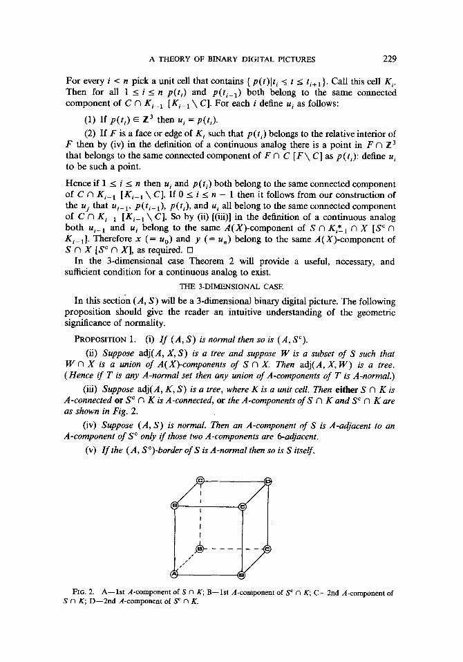
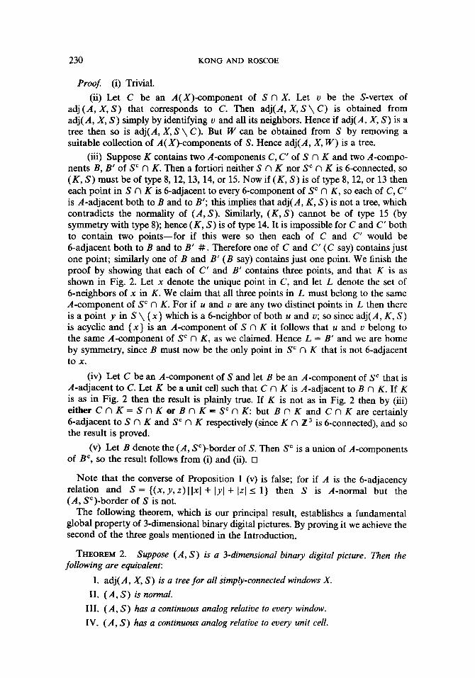
(iii) Suppose adj(A, K, S) is a tree, where K is a unit cell. Then either S N K is A-connected or S ~ n K is A-connected, or the A-components of S n K and S ~ n K are as shown in Fig. 2.

(iv) Suppose ( A, S) is normal. Then an A-component of S is A-adjacent to an A-component of S ~ only i f those two A-components are 6-adjacent.

(v) I f the ( A, SC)-border of S is A-normal then so is S itself.

L I

I

I

11 r f

FIG. 2. A--lst A-component of S O K; B--lst A-component of S c N K; C--2nd A-component of S n K; D--2nd A-component of S c n K.

230 KONG AND ROSCOE

Proof (i) Trivial.

(ii) Let C be an A(X)-component of S n X. Let v be the S-vertex of adj (A, X , S ) that corresponds to C. Then adj(A, X , S \ C ) is obtained from adj(A, X, S) simply by identifying v and all its neighbors. Hence if adj(A, X, S) is a tree then so is adj(A, X, S \ C). But W can be obtained from S by removing a suitable collection of A(X)-components of S. Hence adj(A, X, W) is a tree.

(iii) Suppose K contains two A-components C, C' of S n K and two A-components B, B ' of S c O K. Then a fortiori neither S n K nor S c O K is 6-connected, so (K, S) must be of type 8, 12, 13, 14, or 15. Now if (K, S) is of type 8, 12, or 13 then each point in S N K is 6-adjacent to every 6-component of S c O K, so each of C, C' is A-adjacent both to B and to B'; this implies that adj(A, K, S) is not a tree, which contradicts the normality of (A, S). Similarly, (K, S) cannot be of type 15 (by symmetry with type 8); hence (K, S) is of type 14. It is impossible for C and C' both to contain two points--for if this were so then each of C and C' would be 6-adjacent both to B and to B' # . Therefore one of C and C' (C say) contains just one point; similarly one of B and B' (B say) contains just one point. We finish the proof by showing that each of C' and B' contains three points, and that K is as shown in Fig. 2. Let x denote the unique point in C, and let L denote the set of 6-neighbors of x in K. We claim that all three points in L must belong to the same A-component of S r n K. For if u and v are any two distinct points in L then there is a point y in S \ (x} which is a 6-neighbor of both u and v; so since adj(A, K, S) is acyclic and { x } is an A-component of S r K it follows that u and v belong to the same A-component of S c n K, as we claimed. Hence L = B' and we are home by symmetry, since B must now be the only point in S c o K that is not 6-adjacent to x.

(iv) Let C be an A-component of S and let B be an A-component of S ~ that is A-adjacent to C. Let K be a unit cell such that C o K is A-adjacent to B n K. If K is as in Fig. 2 then the result is plainly true. If K is not as in Fig. 2 then by (iii) either C A K = S A K o r B A K = S o A K : but B A K and C A K are certainly 6-adjacent to S N K and S ~ n K respectively (since K n Z 3 is 6-connected), and so the result is proved.

(v) Let B denote the (A, SC)-border of S. Then S ~ is a union of A-components of B ~, so the result follows from (i) and (ii). []

Note that the converse of Proposition 1 (v) is false; for if A is the 6-adjacency relation and S = {(x, y, z) l lx l + lyl + Izl -< 1} then S is A-normal but the (A, S~)-border of S is not.

The following theorem, which is our principal result, establishes a fundamental global property of 3-dimensional binary digital pictures. By proving it we achieve the second of the three goals mentioned in the Introduction.

THEOREM 2. Suppose ( A, S) is a 3-dimensional binary digital picture. Then the following are equivalent:

I. adj(A, X, S) is a tree for all Simply-connected windows X.

II. (A, S) is normal.

III. ( A, S) has a continuous analog relative to every window.

IV. ( A, S) has a continuous analog relative to every unit cell.


Proof. I implies H; I l l implies IV. These implications are trivial.

H implies 111. Suppose II holds. Let X be a simply-connected window. For each unit cell K contained in X we shall construct a closed polyhedral set C(A, K, S) which is a continuous analog of (A, S) relative to K. C(A, K, S) is defined as follows:

1. If every comer of K belongs to S then C(A, K, S) = K; if every comer of K belongs to S c then C(A, K, S) -- { }.

2. If S c n K is non-empty and A-connected then C(A, K, S) is the union of S o K with all faces of K whose four comers are all in S, all (1,1, ~/2) triangles whose comers are all in S N K, and all straight line segments whose endpoints are comers of K that belong to the same A-component of S n K x for some unit cell g 1 ___ K* n S .

3. If S~A K is not A-connected and ( K , S ) is not of type 14 or 15 then C( A, K, S) = co( S n K ). (Note: co = "convex-hull of".)

4. If SeN K is not A-connected and (K,S) is of type 14 or 15 then let r, s, t, u, v,w, x, y, z denote the points with coordinates (�89 �89 �89 (0, 0, 0), (0, 0, 1), (0, 1, 0), (1, 0, 0), (1, 1, 0), (0,1,1), (1, 0,1), (1, 1,1), respectively. C(A, K, S) is defined by the following five rules:

(A) If each point in K n S ~ belongs to a different A-component of S ~ n K then we define C(A, K, S) = co(S N K).

(B) If (K, S) is of type 15 and S c O K has exactly two A-components then let p be a rotation which maps these A-components onto the sets { s, y } and { w }. We define C(A, K, S) = p - l ( c o ( { l , u, x, g}) U co( ( u, v, 2}) U co({t, v})).

(In (C), (D), and (E) (K, S) is assumed to be of type 14.)

(C) If S c n K has exactly three A-components then let p be a rotation which maps these A-components onto the sets {u}, {v}, and (t, z}. We define C(A, K, S)

= p-l(co((s, w, y)) u co((s, w, x}) u co((x, y})). (D) If S ~ n K has two different A-components and each of them contains just

two points then let p be a rotation which maps these A-components onto the sets {t ,v} and {u,z}. We define C(A,K ,S )=p- l ( co ( { s , x , r } )Oco({s ,w , r } )U co({y, w, r}) O co({x, y, r}) O co({s, y}) U co({x,w))).

(E) If one A-component of S ~ n K contains three points and a second A-component of S r O K contains just one point then let p be a rotation which maps these two A-components onto the sets { v } and { t, u, z }. Let R be the subset of { s, y, w } consisting of those comers which belong to the same A-component of S O K~ as x for some unit cell K 1 _ K* n X. We define C ( A , K , S ) = p- l (co({s ,y ,w})u L) where L is the union of all straight line segments with one endpoint at x and one endpoint in R.

We claim that C(A, K, S) satisfies (i), (ii), (iii), (iv), and (v) in the definition of a continuous analog relative to K. This is easily confirmed in cases 1, 2, and 4. (Note that in (A), (B), (C), and (D) of case 4, Proposition 1 (iii) implies that S o K is A-connected.) Now suppose case 3 applies. Then (i), (iv), and the first assertions of (ii) and (iii) are plainly satisfied; furthelxnore, Proposition 1 (iii) implies that S n K is A-connected, so since C(A, K, S) is convex (and hence connected) (ii) holds. By inspection of Fig. 1 we see that if (K, S) is not of type 14 or 15 then there are at

232 KONG AND ROSCOE

most two 6-components of S c n K, so by the hypotheses of case 3, two points in S c n K belong to the same A-component of S e n K iff they belong to the same 6-component of S ~ n K. Further inspection of Fig. 1 reveals that if (K, S) is not of type 14 or 15 then each connected component of K \ c o ( S n K ) meets Z 3 in a 6-component of S e n K. Hence (iii) holds. We now know that C(A, K, S) is a connected set which meets Z 3 in just one A-component of S n K, and that each connected component of K \ C(A,K, S) meets Z 3 in just one A-component of S ~ n K; so since the boundary of C(A, K, S) must meet the boundary of each component of K \ C(A, K, S) and C(A, K, S) O Z 3 must be A-adjacent to each A-component of ( K \ C(A, K, S)) N 13, it follows that (v) also holds.

Define C = U(C(A, K, S)IK is a unit cell contained in X) . Observe that, by our construction of C(A, K, S), we have C(A, K, S) = C n K for every unit cell K contained in X. So since C(A, K, S) is a continuous analog of (A, S) relative to K, it follows that C is a continuous analog of (A, S) relative to X, and this proves that II implies III.

1V implies H; III implies L Suppose (A, S) has a continuous analog relative to a simply-connected window X (thus X might be a unit cell or the whole of R 3). We shall show that adj(A, X, S) is a tree. Suppose (for the purpose of getting a contradiction) that adj(A, X, S) contains a cycle. Let U and V be distinct A-components of S c n X which correspond to two vertices on the cycle. Pick a point u in U and a point v in V.

By definition of u and v we may partition S n X into two subsets M and N such that each of M and N is a union of A-components of S N X and such that there exist A-paths Po in X O M c and Qo in x N N c each of which links u to v. Now let C be a continuous analog of (A, S) relative to X. By Proposition 0(i) there exist closed sets F and B, each of which is a union of connected components of C, such that F O Z 3 = M and B O 13 = N. By conditions (ii), (iii), and (v) of the definition of a continuous analog u and v are connected in X \ F and in X \ B. X \ F and X \ B are both open relative to X, so there exist two curves "/0 and Y1 in X joining u to v such that the trace of ~'0 does not meet B and the trace of 3'1 does not meet F.

By our definition of simple-connectedness there exists a continuous map h: [0,1] • [0, 1] --* X such that for all s and t in [0, 1]:

(i) h(s,O) = Vo(S) (ii) h(s, ] ) = v l ( s )

(iii) h (0, t) = u

(iv) h(1, t) = v.

In the rest of this proof the term "square" denotes a closed 2-dimensional square (and not just the interior or boundary of the "square"). By "drawing" lines parallel to the x and y axes we may dissect the unit square [0, 1] • [0,1] into n 2 little squares of side l/n, where n is chosen so large that the image under h of each little square always misses at least one of the two sets F and B. Let Q be the set of all the little squares whose image under h meets F. Define E o = {ele is an edge of exactly one square in Q }. Let L denote the straight line segment with endpoints (0, 0) and (1,0) and let E 1 denote the set {ele is an edge of a little square and e c L}. Let E denote the symmetric difference of E 0 and E x. With the exceptions of (0, 0) and (1, 0) each comer of a little Square is incident either on no edges in E or on exactly


two edges in E. Each of (0, 0) and (0,1) is incident on exactly one edge in E. It follows that (0, 0) and (0,1) belong to the same connected component of UE; call this connected component P. Then h(P) is a connected subset of X which contains both u and v but does not meet F or B. So since X \ C is open in X there exists a simple polygonal arc in X \ C which joins u and o. So by Proposition 0, u and o belong to the same A-component of S ~ n X, which is the required contradiction. []

Theorem 2 implies that if a closed set has a digital representation then all its digital representations are normal. Another easy corollary is the following generali- zation of Corollary 7 in [15].

COROLLARY. Suppose one of a and fl is not equal to 6. Then adj(a, fl, S) is a tree for every S.

Proof. By definition adj(a, fl, S) = adj(A(a, fl, 6, S), S). But we have already noted that (A(a , fl, 3', S), S) is normal whenever a and fl are not both equal to 6; so the corollary follows from the theorem. []

Remark. Theorem 2 remains true if property I is replaced by the more general assertion:

I ' : For all windows X the Euler characteristic of adj(A, X, S) is not less than the Euler characteristic of X minus the number of cavities of X.

(This says that adj(A, X, S) never has more "holes" than X. Thus if X has just one hole then "adj(A, X, S) has at most one cycle.)

Proposition 1 (ii) implies that if (A, W) is normal then every A-component of W is A-normal. The converse of this result is false; indeed, if A is the 6-adjacency relation and S = ((x, y, z) I lxl + lYl + Izl = 1} then adj(A, S) is the complete bipartite graph K(6, 2) which is not a tree. However, a partial converse is provided by the corollary to the following proposition.

PROPOSITION 3. Let X be a window, and let ( A, T) be a binary digital picture such that adj(A, X, T) is a tree. Let {T,.10 < i < n} be the set of A-components of T n X and let W be a subset of T such that for each i the adjacency graph adj(A, X, T/O W) is a tree. Then adj(A, X, W) is a tree.

Proof. Suppose the hypotheses are satisfied but adj(A, X, W) contains a cycle F. Let W~ denote T~ n X. We shall deduce the contradiction that for some i adj(A, X, W~) contains a cycle. Let a, x, and b be three consecutive vertices on F such that x is a W vertex, and let T O be the A-component of T n X that contains COMPT(x). Thus COMPT(x) is an A-component of W n X while COMPT(a) and COMPT(b) are A-components of W c n X. Now COMPT(a) and COMPT(b) are both A-adjacent to COMPT(x), but since I" is a cycle they are not separated by COMPT(x). So since by assumption adj(A, X, W0) is a tree it follows that COMPT(a) and COMPT(b) are contained in the same A-component of W~ n X.

Pick u and v on the (A, COMPT(x))-borders of COMPT(a) and COMPT(b), respectively. By the last sentence in the previous paragraph there exists an A-path P in X which joins u to o and which does not meet W 0. Now a ~ : b means COMPT(a) and COMPT(b) are different A-components of W e n X. Hence P contains at least one point in W and since P does not meet W 0 = T O O W it follows that every point w in W that lies on P belongs to ( T \ To). For every point w in W that lies on P let z (w) and z '(w) denote the two points on P which are such that:

234 KONG AND ROSCOE

(a) z(w) and z'(w) both lie in To; (b) z(w) comes before w and z'(w) comes after w on P; (c) the portion of P between z(w) and z'(w) contains no other points in T 0. Also, let r(w) denote the immediate successor of z(w) on P and let s(w) denote the immediate predecessor of z'(w) on P. Suppose temporarily that there is no point w such that r(w) and s(w) belong to different A-components of T c n X. Then we can construct an A-path P ' in ( T 0 \ W) U (T r n X) that joins u to v - P ' passes through each r(w) and s(w) but bypasses every point w in W that lies on P. The A-path P ' does not meet W, which implies that a = b # . This contradiction shows that there must exist a point w 0 such that r(wo) and S(Wo) belong to different A-components of T c. But by construction r(Wo) and S(Wo) are both A-adjacent to T 0, and they are not separated by T 0. Hence adj(A, X, T ) contains a cycle and this contradiction proves the proposition. []

COROLLARY. Let T be an A-normal set and let W be a subset of T which meets each A-component of T in an A-normal set. Then W is A-normal.

Proof. Let K be an arbitrary unit cell and let T O be any A-component of T n K. Let T 0' be the A-component of T that contains T 0. Then adj(A, K, TO' N W) is a tree, so by Proposition 1 (ii) adj(A, K, T O N W) is a tree. Also, adj(A, K, T) is a tree since T is A-normal. So since T O was any A-component of T n K Proposition 3 implies that adj(A, K, W) is a tree. This argument works for all unit cells K, so W is A-normal. []

We are now ready to prove a very general result on the connectivity of digital borders. Basically, we give conditions which ensure that the border of a component of object points with respect to a component of background points is connected and separates the components. If any digital picture contains a border which does not have these two properties then it is clear that the adjacency relation is incompatible with the set of object points.

PROPOSITION 4. Let F and B be A-components of S and S ~ respectively and let W denote the (A, B)-border of F. Suppose both S and W are A-normal. Then W is A-connected. Furthermore, if W is non-empty and P is an A-path linking a point in F to a point in B then there are two consecutive points u, o on P such that u ~ W and v ~ B .

Proof. Let T denote the set W w (S \ F) . Suppose W is not A-connected. Let U and V be distinct A-components of W. Then there exists an A-path in F that links U to V; on such an A-path pick a point x that does not belong to W, and let X denote the A-component of T r that contains x. U and V are distinct A-components of T. Furthermore, B is an A-component of T c and B ~ X. Now there exist two A-paths Po and Pt from x to B such that P0 goes through V and does not meet U while Px goes through U and does not meet V. It follows that there exist two different paths in adj(A, T) from X to B (of which one contains U and the other contains V). But R 3 is a simply-connected window; therefore Theorem 2 implies that T is not A-normal. But, by the corollary to Proposition 3, T is A-normal since T meets each A-component of S is an A-normal set. This contradiction proves the first assertion.

To prove the second assertion suppose W is non-empty, and let z be any point in F. If z ~ Wdef ine C = W; if z ~ F \ W then let C be the A-component of T ~ that contains z. Let P be an A-path from z to a point in B. Let b, c, and w be the


vertices of adj(A, T) such that COMPT(b) = B, COMPT(c) = C, and COMPT(w) = W, so that w is adjacent to b and either w = c or else w is adjacent to c. We have already noted that T is A-normal, so adj(A, T ) is a tree. Now the A-path P induces a walk in adj(A, T ) from c to b, and this walk must traverse the edge in adj(A, T) joining w to b (since adj(A, T) is acydic). This implies the result. []

The next proposition is the analog of Proposition 4 in the conventional theory of binary digital pictures (as described in [15 or 16]). The proposition contains Proposition 5 in [15] as a special case and can also be shown to imply the principal theorem in [6] (use the technique described in the final section of [10]). So by proving it we achieve the third and last of our goals. Results of this kind are used to establish the soundness of border-tracking algorithms.

PROPOSITION 5. Leg each o f a, fl, and ~ be equal to 6, 18, or 26, and let 8 = min( f l , u Le t F be an a-component o f S, let B be a fl-component o f S c, and let W denote the (y, B)-border of F:

(i) Suppose at least one of a and 8 is not equal to 6. Then W is a-connected.

(ii) Suppose W is non-empty and at least one of a and fl is not equal to 6. Then any 8-path P f rom a point in F to a point in B contains two consecutive points u, v such that u ~ W and v ~ B.

Proof. Case I: a and 8 are not both equal to 6. We shall prove (i) and (ii) simulta-

neously. Let A denote the adjacency relation on Z 3 such that x and y are A-adjacent

either if they are A ( a , fl, y, S)-adjacent or if x and y are 26-neighbors in S \ W. Observe that B is an A-component of S c.

Let K be any unit cell. If a = 6 (so that nefther fl nor ~, is equal to 6) then either S n K is 6-connected (and hence A-connected) or else S r n K is 18-connected (and hence A-connected). If on the other hand a 4 :6 then either S N K is 18-connected (and hence A-connected) or else S r O K is 6-connected (and hence A-connected). Thus S is A-normal in all cases.

Let F ' denote the A-component of S that contains F, and let IV' denote the (A, B)-border of F ' . Let K be any unit cell. If a = 6 (so that neither 13 not ~, is equal to 6) then either W' N K is 6-connected (and hence A-connected) or else W 'c t~ K is 18-connected (and hence A-connected). If on the other hand a 4:6 then either W' n K is 18-connected (and hence A-connected) or else W 'c n K is 6-connected (and hence A-connected). Thus W' is A-normal in all cases. Recalling that S is also A-normal, we see that by Proposition 4 the set W ' is A-connected. But it is easy to see that W = IV' r F, so that W is a subset of W' that is not A-adjacent to W ' \ W. Hence W = IV'. This proves part (i) of the proposition. Since W is A-connected it follows that given any &path P we can construct an A-path P ' which agrees with P except possibly on W (in the sense that if x and y are consecutive points on P which are not both in W then x and y are consecutive points on P ' , and vice versa). Thus we are home by Proposition 4 (applied to A, F' , B, and VII' = W ).

Case H: a = 6 and 8 = 6. Here only part (ii) of the proposition applies. Note that fl 4 :6 (by the hypothesis that at least one of a and fl is not equal to 6), and so "t = 6. Let P be a 8-path (i.e., a 6-path) from a point in F to a point in B. Let W "

236 KONG AND ROSCOE

be the (26, B)-border of F and let 8' = min(/3, 26) =/3. Then since the 6-path P is (a fortiori) a 8'-path, and since 8' ~ 6 it follows from Case I that there are two consecutive points u, v on P such that u ~ W" and v ~ B. But u ~ W'" implies u ~ F, and, since u and v are consecutive on P, u is 6-adjacent to the point v, which is in B. Hence u ~ W, and we are home. D

We can show that Proposition 5 is a "best possible" result. First of all, it is obvious that W will not in general be more than a-connected, simply because that is the only sort of connectivity that is assumed for F. Now put S = X U Y U ( ( 2 , 0 , 0 ) , ( - 2 , 0 , 0 ) } where X = { ( x , y , z ) ~ Z3lmax(lx[, [y[, Izl) = 3 and just one of Ixl, lYl, Izl is equal to 3}, and Y = ((x, y, z) ~ Z31 Ixl + lYl + Izl -< 1}. We shall consider the consequences of different choices of a , /3 , and 7. In all cases let B denote the only unbounded/3-component of S c, let z 0 be the point (0, 0, 0), let F denote the a-component of S that contains z0, and let W denote the (7, B)-border of F. If a = 8 = 6 then W is not a-connected, so part (i) fails; if ot = /3 = 6 then z 0 is contained in the same 8-component of W c as B so part (ii) fails. Also, part (ii) cannot be strengthened by substituting/3 or 7 for 8: If a = /3 = 18 and 7 = 6 then z o is contained in the same/3-component of W c as B while if a = 7 = 18 and 13 = 6 then z o is contained in the same 7-component of W ~ as B. Even if ~ = 18, part (ii) may fail if 8 is replaced by /3 or 7- To see this put (fl, 7) = (26,18) or (18, 26) S = F = X \ Y, where X = ( ( x , y , z ) ~ Z31max(Ixl, lYl, Izl) -< 2) a n d Y = {(x, y, z) ~ 131 Ix[ = lyl = Izl >- 1}.

THE 2-DIMENSIONAL CASE

It is easily seen that Proposition 1 remains true in two dimensions (in part (iv) "6-adjacent" should be replaced by "4-adjacent," and the assumption that (A, S) is normal is unnecessary).

Unfortunately Theorem 2 fails when (A, S) is a 2-dimensional binary digital picture; indeed, if S = { ( x , y ) ~ 121 Ixl + l Y l - - 1 } and A is the 8-adjacency relation then (A, S) is normal but has no continuous analog. (The fact that (A, S) has no continuous analog is the essence of the "paradox" mentioned in ([17, p. 475]). If S is as above and A is the 4-adjacency relation then (A, S) again has no continuous analog--this can be regarded as the source of the "Euler theorem paradox" mentioned in ([14, p. 147]), where these paradoxes are put forward as a reason for not "using the same type of connectivity for both set and complement." But note that in the second case (A, S) is not normal, and so would not be expected to have a continuous analog.) It is easy to prove the following weak analogy of Theorem 2:

THEOm~M 2'. Suppose ( A, S ) is a 2-dimensional binary digital picture. Let four conditions I, 11, 111, and I V be defined as follows:

I. adj(A, X, S) is a tree for all simply-connected windows X.

II. (A, S ) is normal.

III. ( A, S ) has a continuous analog relative to every window.

IV. ( A, S ) has a continuous analog relative to every unit cell. Then I and 11 are equivalent, I I I and I V are equivalent, and 111 and I V imply ! and H.

Proof. Let (A, S) be a 2-dimensional binary digital picture. It is readily confirmed that if for every unit cell K the set C(K) is a continuous analog of (A, S)


relative to K then for every window X the set U{C(K)IK c__ X} is a continuous analog of (A, S) relative to X. Hence III and IV are equivalent. Now define an adjacency relation A' on Z 3 such that two points (x ,y , z ) and (x ' ,y ' ,z ' ) are A'-adjacent iff they are 26-adjacent and the points (x, y) and (x', y') are either equal or A-adjacent. Define S' to be the set S • {0,1}. Then if X is any 2-dimensional window we have that adj(A, X, S) is a tree if and only if adj(A', X • [0,1], S') is a tree (here [0,1] denotes the closed unit interval {x I 0 < x < 1}). Hence I and II are equivalent by Theorem 2. Moreover, if C is a continuous analog of (A, S) relative to X then C • [0, 1] is a continuous analog of (A', S') relative to X • [0,1]. So IV implies II by Theorem 2. []

Remark. In this paper we never actually make use of the assumption that an n-dimensional window is actually embedded in n-dimensional Euclidean space. Thus one might define a generalized window to be any space obtainable by taking a disjoint collection of unit cells and "gluing together" some of the corners, edges and (in three dimensions) faces of these cells. Observe that any union of faces of 3-dimensional unit cells is a 2-dimensional generalized window, regardless of whether or not the faces all lie in one plane. Theorems 2 and 2' remain valid if X is a generalized window.

Propositions 3 and 4 remain true in two dimensions: the proofs are obtained from the 3-dimensio.nal proofs by replacing references to Theorem 2 by references to Theorem 2'. If in the statement and proof of Proposition 5 we replace "26" and "18" by "8", and we replace "6" by "4" then we get a correct statement and proof of a 2-dimensional version of Proposition 5. This is again a "best possible" result--2-dimensional versions of the examples given after the proof of Proposition 5 are easily constructed.

THE HEXAGONAL AND FACE-CENTRED CUBIC LATTICES

It is unfortunate that, in general, neither of the 2-dimensional binary digital pictures (4, S) and (8, S) has a continuous analog relative to any given window; the same applies to the 3-dimensional picture (6, S). As a result, digital objects in these pictures can have properties which real objects never have--recall the counterexam- pies given after the proof of Proposition 5. Although continuous analogs always exist for the binary digital pictures (18, S) and (26, S) (because they are always normal) these continuous analogs do not always reflect the topological structure of the picture. As an example, consider the digital picture (a, {(0,0, 0), (1, 1, 0),(0, 1, 1)}), where a = 18 or 26: although one feels that this digital picture ought to be simply connected, since any two object points are mutually adjacent, it does not have a simply-connected continuous analog (relative to R 3). A related problem is that if we define the Euler characteristic of (18, S) and (26, S) to be the Euler characteristic of the natural continuous analogs of these pictures, then the topological structure of a picture may change when a simple point (defined in [9]) is removed. A much more obvious drawback of (18, S) and (26, S) is that the 18- and 26-adjacency relation give each point too many neighbors: it is desirable to have fewer neighbors, as this will reduce the amount of computation involved in many algorithms.

The standard way of avoiding these difficulties is to use adjacency relations of the form A(a, fl, fl, S), where S is the set of object points, and exactly one of a and fl (usually fl) is equal to 4 or 6. This approach was suggested by Duda [4]. But in both two and three dimensions there is an elegant alternative.

238 KONG AND ROSCOE

In the 2-dimensional case this alternative is in fact quite well known, although it has never been widely used in practice. It involves abandoning the rectangular grid in favor of the hexagonal lattice which is constructed by tessellating the plane with unit equilateral triangles and regarding each point lying at a corner of a triangle as a lattice-point. The hexagonal lattice is so called because it is possible to tessellate the plane with regular hexagons in such a way that the set of lattice-points is exactly the set of centers of the hexagons.

The only adjacency relation we shall use with this lattice is the relation A such that each lattice-point is A-adjacent to its six nearest neighbors and to no other points. A binary digital picture on the hexagonal lattice is just a set of lattice-points (since the adjacency relation is fixed there is no need to include it in the definition). The relation A assigns just 6 neighbors to each lattice-point, which is an improvement on the 8-adjacency relation on the rectangular lattice. Actually, the hexagonal lattice has another advantage over 8-adjacency: in the hexagonal lattice each lattice-point is equidistant from all its neighbors. More generally, the adjacency relation A is isotropie in the sense that if p, q, and r are any three lattice-points in the hexagonal lattice such that p and q are both adjacent to r then there is a plane rotation with center r which preserves the lattice and maps p to q.

Digital pictures on the hexagonal lattice can be incorporated into the theory of digital pictures developed above. Indeed, if A' denotes the adjacency relation on the rectangular lattice Z 2 such that (x, y) is A'-adjacent to (s, t) iff (x, y) is 4-adjacent to (s, t) or (x - s, y - t) ~ {(1, 1), ( - 1, - 1)}, then there is an afline map T of the plane to itself which induces a bijection of the points of the hexagonal lattice to Z 2 with the property that two lattice-points in the hexagonal lattice are A-adjacent iff their images in the rectangular lattice are A'-adjacent. So for the purposes of digital topology every binary digital picture W on the hexagonal lattice is equivalent to the binary digital picture (A', T(W)) on the rectangular lattice.

It is readily confirmed that (A ' ,S ) is normal for all S. Moreover, a very well-behaved continuous analog for (A', S) relative to an arbitrary window X can be constructed by taking the union of all points in S n X, all straight line segments joining two A'-adjacent points in S n X, and all (1,1, r triangles each of whose sides joins two A'-adjacent points in S n X. Thus the "borders are connected and surround" result (Proposition 4) holds for digital pictures on a hexagonal lattice. Note that this is a property of the hexagonal lattice itself, and not merely a property of A'.

The 3-dimensional analog of the 2-dimensional hexagonal lattice is the face- centered cubic lattice whose set of lattice-points can be taken to be ((x, y, z) ~ Za[ x + y + z is even}. The only adjacency relation we shall use with this lattice is the relation A 1 in which each lattice-point is adjacent to its nearest neighbors. As the adjacency relation is again fixed we can define a binary digital picture on the lattice to be any set of lattice-points. The adjacency relation A 1 assigns 12 neighbors to each lattice-point, which is an improvement on the 18- or 26-adjacency relations on the rectangular lattice. Like the adjacency relation A on the 2-dimensional hexagonal lattice the adjacency relation A1 is isotropic, which the 18- and 26-adjacency relations are not.

It is interesting to note that there we can tessellate 3-space with equal rhombic dodecahedra in such a way that the set of centers of the rhombic dodecahedra is exactly the points set of the face-centered cubic lattice. (The convex polyhedron


whose vertex set is ( ( x , y , z ) ~ Zallxl + lYl + Izl = 2 and IxllYl + Izl > 0} is a rhombic dodecahedron.)

As in the case of the hexagonal lattice, digital pictures on the face-centered lattice can be incorporated into our general theory. There are two natural ways of doing this. The first way is based on the adjacency relation A t on the rectangular grid such that the point (x, y, z) is A~-adjacent to the point (t, u, v) if and only if the two points are 6-adjacent, or (x - t, y - u, z - v) ~ {(1, 0, 1), (0,1, 1), ( - 1,1, 0), ( - 1, 0, - 1), (0, - 1, - 1), (1, - 1, 0)}. The other way is based on the adjacency relation A t' on the rectangular grid such that the point (x, y, z) is A~'-adjacent to the point (t, u, o) if and only if the two points are 6-adjacent, or (x - t, y - u, z - v) {(1 ,0 ,1) , (0 ,1 ,1) , (1 ,1 ,1) , ( -1 ,0 , - 1),(0, - 1 , - 1 ) , ( - 1, - 1 , - 1 ) ) .

There are affine transformations T{ and T~' which map the points of a face- centered cubic lattice onto the points of a rectangular lattice in such a way that two points of the face-centered cubic lattice are At-adjacent ill their images under T t' and TI" are respectively At-adjacent and A~'-adjacent. So for the purposes of digital topology every binary digital picture on the face-centered cubic lattice is equivalent to binary digital pictures on the rectangular lattice based on the adjacency relations A t and At'.

We claim that (At, S) and (At', S) are normal for all S. To justify this claim, it suffices to show that each of adj(A i, K, S) and adj(A~', K, S) is a tree when K is the unit cell that contains (0, 0, 0) and (1,1,1). We may assume w.l.o.g. (by symmetry between S and S c) that (0, 0, 0) ~ S. If (1, 0, 0) or (0,1, 0) is also in S then S n K is At-connected so adj(A{, K, S) is a tree. If both of these points are in S c then the set consisting of these two points (which are contained in one At-component of S c n K) is At-adjacent to every At-component of S n K. Moreover, if there is a second At-component of S r N K then it must be ((0, 0, 1)} (since all other points in S c n K are At-adjacent to (1, 0, 0) or (0,1, 0)), and {(0, 0,1)} is adjacent to only one Ai-component of S n K. So adj(A{, K, S) is a tree in all cases. Again, if one of the three points (1, 0,0), (0,1,0), and (1,1,1) is in S then S n K is Ai'-connected, whence adj(Ai' , K, S) is a tree. If all three of these points are in S c then the set consisting of these three points (which are contained in one Ai'-component of S c N K ) is Ai'-adjacent to every Ai'-component of S n K. Moreover, if there is a second Ai'-component of A c n K then it must be {(0, 0,1)}, which is Ai'-adjacent to only one A{'-component of S N K. So adj(Ai', K, S) is a tree in all cases.

It follows that the "borders are connected and surround" result (Proposition 4) holds for digital pictures based on the face-centered cubic lattice. Although this result is proved by consideration of A t (or At' ), it expresses a property of the face-centered cubic lattice itself.

Moreover, it turns out that for all S the digital pictures (At, S) and (Ai', S) have well-behaved continuous ~malogs relative to every window, which meet each unit cell in a simply-connected set. The construction of such continuous analogs is not hard; but it does involve a certain amount of case analysis and will not be described here.

CONCLUDING REMARKS

This paper may be summarized as follows:

(a) We introduced a new definition of a binary digital picture (based on the lattice-point representation of voxels); the new definition was more general but at the same time rather simpler than the definition used in [15].

240 KONG AND ROSCOE

(b) We adapted Rosenfeld's adjacency graphs to the new definition, and at the same time introduced the slightly broader concept of the X-adjacency graph of a binary digital picture, where X can be any window (i.e., any union of unit cells).

(c) We defined a normal binary digital picture to be a picture (A, S) whose K-adjacency graph is a tree for every unit cell K.

(d) We introduced the notion of the continuous analog of a binary digital picture relative to a window.

(e) Using the method of continuous analogs, we proved satisfying theorems (Theorems 2 and 2'), which show that the concept of normality is of fundamental importance in the theory of binary digital pictures.

(f) Two results (Propositions 4 and 5 and their 2-dimensional variants) concern- ing the connectedness of digital borders were deduced from Theorems 2 and 2' (without making further use of the powerful but rather complex machinery of continuous analogs). These results are general forms of Proposition 5 in [15] and they are useful for proving the soundness of border tracking algorithms.

(g) We showed how binary digital pictures on the hexagonal and face-centered cubic lattices with nearest neighbor adjacency could be incorporated into the theory, and explained why they are well behaved.

Our approach to digital topology (based on the new definition of a binary digital picture) produces stronger theorems than the conventional approach described in [15]. Thus no result as powerful as Theorem 2 could be stated in terms of the old theory, and so it would be impossible to prove a result like Proposition 5 in the way we have. The relationship of our approach to previous ones is akin to that between the study of topology and the study of particular topological spaces. The generality of our approach has paid off in the applications ((f) and (g) above) which have emerged.

The new theory could have other, more practical, advantages too. Suppose we wished to extract "connected components" of S--which in one context (see [2]) might correspond to organs in a human body. Then we would use an algorithm which finds A-components of S, where many different choices of the adjacency relation A are acceptable. This is a well-known example of a family of algorithms that is naturally parameterized by a set of "possible choices" of adjacency relation. The new theory can cope with a greater variety of different adjacency relations than the old theory and this increased power might have applications in situations where our pictorial data is "noisy" and of low resolution.

Finally, this paper provides a second illustration (following [7]) of how continuous methods can be used to prove deep results in digital topology.

APPENDIX

A. Simple-Connectedness

In most texts (e.g., [1]) a connected set Y is said to be simply-connected iff every closed curve in Y can be continuously deformed to a single point. Thus Y is simply connected ill given any curve ,/: [0,1] ~ Y such that ,/(0) = -/(1) there exists a


cont inuous funct ion h: [0,1] • [0,1] ~ Y with the f o l l o ~ n g properties:

(i) h(x,O) = .t(x) (0 < x < 1),

(ii) h(x , 1) = p (0 < x < 1), where p is a point in Y and is the same for all x,

(iii) h(0, t) = h(1, t) (0 < t < 1).

We shall call this the standard definition. If Y is s imply-connected according to our earlier definition then it is readily seen

to be s imply-connected in the standard sense. To prove the converse suppose Y satisfies the s tandard definition and suppose "to and .t~ are two curves on Y such that .to(0) = .tl(0) and .t0(1) = .tl(1). We must prove the existence of a fixed endpoint h o m o t o p y H of .to onto .tl.

Define a closed curve .t such that . t ( x ) = .to(2X) if x ~ [0 ,1 /2 ] and . t ( x ) = ,/1(2(1 - x ) ) if x ~ [1 /2 ,1] . By hypothesis there exists a cont inuous function h satisfying (i), (i_i), and (iii) above. Now define go, gl, Go, G1, H: [0,1] x [0,1] ~ Y such that:

g o ( x , t ) - h ( x / 2 , t); g l ( t ) = h(1 - x / 2 , t ) ; f o r j = 0 ,1 ,

Gj(x , t) = gj(O, 2 x ) if x < t /2 ,

Gj(x , t . ) = g j (1 ,2 (1 - x ) ) i f x >__ 1 - t / 2 ,

Gj(x , t) = g j ( (2x - t ) / ( 2 ( 1 - t ) ) , t ) otherwise;

H ( x , t) = Go(x, 2t ) if t _< 1 / 2 ,

H ( x , t ) = Gl (X ,2 (1 - t ) ) if t >__ 1 / 2 .

Then

H(x,O) = . to(X);

H ( x , 1) = . t l (X);

H(0 , t ) = Y0(0) - . t l(0);

H(1 , t ) - .t0(1) = .tl(1).

I t is easily verified that G is continuous. (The only point where there is any doubt is (�89 which is a discontinuity of (2x - 0 / ( 2 ( 1 - t)); however, all is well because gj is uni formly cont inuous ( j = 0,1): given any t > 0 we can pick 8 > 0 so small tha t whenever t > 1 - ~ the distance between gj(x, t) and p is at mos t e, irrespec- tive of the value of x.) Hence H is cont inuous and so H is a fixed endpoint h o m o t o p y that takes .t0 to .tl.

This p roof looks complicated until one realizes the geometric meaning of G and H.

B. Proof That Fig. 1 ls Complete

We shall work out the number of different ways in which we can color the comers of a cube using two colors (black and white, say), where two colorings are considered to be the same if "one is a rotat ion of the other ." We shall use Polya 's enumerat ion theorem. Readers who are unfamiliar with this result are referred to chapter 8 of [3].

242 KONG AND ROSCOE

Each of the 6 faces of a cube has 4 sides, so there are just 24 different rotations which map a cube onto itself. These 24 rotations can be classified as follows:

1. The identity,

2. A quarter turn (clockwise or anticlockwise) about an axis passing through the centers of two opposite faces (3 x 2 = 6 possibilities),

3. A half turn about an axis passing through the centers of two opposite faces (3 possibilities),

4. A half turn about an axis passing through the mid-points of two diagonally opposite edges (6 possibilities),

5. Rotat ion through an angle of 2~r/3 or - 2~r/3 about an axis passing through two diametrically opposite corners (4 • 2 = 8 possibilities).

The cycle index associated with this group of rotations is (a~ 8 + 6a24 + 3a 4 + 6a~ + 8a2a2)/24. Hence if we associate a weight of 1 with all points, black or white, then Polya's enumeration theorem shows that the number of different colorings is

(28 + 6 • 22 + 3 • 24 + 6 • 24 + 8 • 22 • 22) /24 = 23.

Plainly each of the 22 cells in Fig. 1 corresponds to a different one of these 23 colorings. The only remaining coloring corresponds to a reflection of cell 11. This proves that any unit cell can be mapped by an appropriate rotation either onto one of the cells in Fig. 1 or onto a reflection of cell 11. []

ACKNOWLEDGMENTS

The authors wish to thank Professor C. A. R. Hoare for a number of useful comments which have influenced various parts of this paper. The first author gratefully acknowledges the support of the Science and Engineering Research Council of Great Britain under Research Studentship B 8200186.

REFERENCES

1. T. M. Apostol, Mathematical Analysis, 2nd ed., Addison-Wesley, Reading, Mass., 1974. 2. E. Artzy, G. Frieder, and G. T. Herman, The theory, design, implementation evaluation of a

three-dimensional surface-detection algorithm, Comput. Graphics Image Process. 15, 1981, 1-24. 3. B. Bollobas, Graph Theory: An Introductory Course, Graduate Texts in Math. Vol. 63, Springer-Verlag,

New York, 1979. 4. R. O. Duda et al., Graphical Data-processing Research Study and Experimental Investigation,

AD650926, March, 1967. 5. G. T. Herman and H. K. Liu, Three-dimensional display of human organs from computed tomo-

grams, Comput. Graphics Image Process. 9, 1979, 1-21. 6. G. T. Herman and D. Webster, Surfaces of organs in discrete three-dimensional space, in Mathemati-

cal Aspects of Computerized Tomography (G. T. Herman and F. Natterer, Eds.), Springer-Verlag, Berlin, 1981.

7. T. Y. Kong and A. W. Roscoe, Continuous analogs of axiomatized digital surfaces, Comput. Vision Graphics Image Process. 29, 1985, 60-86.

8. S. Levialdi, Neighbourhood operators: an outlook, in Pictorial Data Analysis (R. M. Haralick, Ed.), NATO ASI Ser. F, No. 4, pp. 1-14, Springer-Verlag, Berlin/Heidelberg, 1983.

9. D. G. Morgenthaler, Three-Dimensional Simple Points: Serial Erosion Parallel Thinning and Skeletoni- zation, TR-1005, Computer Vision Laboratory, University of Maryland, College Park, Md. 20742.

10. D. G. Morgenthaler and A. Rosenfeld, Surfaces in three-dimensional digital images, Inform. and Control $1, 1981, 227-247.


11. J. Mylopoulos and T. Pavlidis, On the topological properties of quantized spaces, (I, II), J. Assoc. Comput. Mach. 18, 1971, 239-254.

12. G. M. Reed, On the characterization of simple closed surfaces in three-dimensional digital images, Comput. Vision Graphics Image Process. 25, 1984, 226-235.

13. G. M. Reed and A. Rosenfeld, Recognition of surfaces in three-dimensional digital images, Inform. and Control 53, 1982, 108-120.

14. A. Rosenfeld, Connectivity in digital pictures, J. Assoc. Comput. Mach. 17, 1970, 146-160. 15. A. Rosenfeld, Three-dimensional digital topology, Inform. and Control 50, 1981, 119-127. 16. A. Rosenfeld and A. C. Kak, Digital Picture Processing, Vol. II, Academic Press, New York, 1983. 17. A. Rosenfeld and J. L. Pfaltz, Sequential operations in digital picture processing, J. Assoc. Comput.

Mach. 13, 1966, 471-494. 18. R. L. Wilder, Topology of Manifolds, Amer. Math. Soc. Colloq. Publ. Vol. 32, Chap. 2, Amer. Math.

Soc. New York, 1949.

Documents

A Theory of Binary Digital Pictures - Department of … THEORY OF BINARY DIGITAL PICTURES 223 is simply-connected if given any two curves in Y with the same endpoints we can transform