@O&7949187 S3.W + 0.00 Prrgamon Jourwl~ Ltd.

A THREE-DIMENSIONAL IMPACT-PEN~T~TION ALGORITHM WITH EROSION

TED BELYTSCHKO and JERRY I. LIN

Department of Civil Engineering, Northwestern University, Evanston, IL 60201, U.S.A.

(Received 7 February 1986)

Abstract-A new interaction algorithm for treating three-dimensional impact-penetration simulations with erosion is presented. This algorithm is based on interactions between slave nodes (projectile) and master elements (target) and no tracking of the sliding interfaces is needed. It employs an assembly of normals to identify the interface surface adaptively so that it can handle eroding elements in both the target and the penetrator. In the interaction algorithm, momentum is exchanged between interacting nodes so that the total momentum is conserved. Examples of three-dimensional cakulations are also given.

1. INTRODUCFION

In simulating thr~-dimensional impact-~netration mechanics problems, algorithms based on inter- actions between master nodes and slave nodes (I,21 are often used. These algorithms require redefinition or tracking of the sliding interfaces once the elements on the contact surfaces are eroded, which is extremely awkward.

A new algorithm which allows arbitrary erosion in the target or projectile is developed. This algorithm handles the interaction by operations on slave nodes (projectile) and master elements (target) and requires no definition of the contact surfaces. The interaction procedure is designed in such a manner that total momentum is always conserved. This may result in some loss of energy, but it is not considered harmful if the interaction nodes contain only a small portion of the total mass.

An isoparametric hexahedral element with eight nodes and 24 degrees of freedom is incorporated with the new algorithm. The stresses and strains are evaluated only at a single point in the element [3,4J. This can result in certain physically unrealistic modes of deformation, known as hourglass modes. These are avoided by the use of hourglass control [5].

Several other important features of this algorithm are:

(I) A cell structure which subdivides the inter- action domain into smaller zones to localize the detailed penetration detection.

(2) A two-step check procedure, consisting of a rough-but-quick check and a precise check, to detect the penetration.

(3) A standard finite element assembly procedure to assign normal directions for the nodes on the sliding surfaces so that the outside inter- acting surfaces of both the target and pene- trator are readily identified regardless of any erosion that takes place on either body.

2. OVERVIEW OF THE ALGORITHM

The basic purpose of this algorithm is to treat the interaction of two bodies with eroding elements. Eroding elements are elements which are destroyed during the course of the computation because of very high strains, which implies that they represent elements of the target or penetrator which have ceased to play a significant role in the physics of the probIem.

Algorithms with eroding elements in three dimen- sions are very difficult to treat within the conven- tional framework of master and slave contact surfacesfl, 21. It is difficult to design algorithms to redefine the contact surfaces when elements are destroyed, particularly in three dimensions. More- over, the comers which are created in the surfaces by the erosion of elements present severe algorithmic difficulties.

Therefore, this new algorithm uses a concept of slave nodes and master elements. One of the two bodies, usually the projectile, is defined by the nodes, hereafter called slave nodes; the second body is defined by elements, called master elements. If a slave node is found to be inside a master element, it is then brought back to an outside surface. In order to deter- mine the outside surfaces, a set of normal vectors is assembled for all master elements as described in Sec. 5. Because of the character of the assembly process, a nonzero normal vector will only result on outside surfaces and will provide an effective average normal to the surface.

The mechanics of the interaction of the two bodies is executed completely through the interaction of the slave nodes with the master elements. The rules of this interaction are as follows.

(1) Slave nodes are not permitted to penetrate master elements,

(2) Whenever penetration of a slave node into a master element is detected, the slave node is

95 C.A.S. 2511-G

96 TED BELYTSCHKO and JERRY 1. Lrs

returned by a projection to the surface of the element it has penetrated and the associated loss of momentum is transferred to the appro- priate nodes of the master element. If a check shows that this projection has not moved the slave node to an exterior surface, the node is moved to the appropriate edge.

The efficacy of this procedure hinges strongly on the use of explicit time integration, since stability requirements then restrict the time step so that the master element which is penetrated effectively repre- sents the zone of the interaction; it should be noted that in cases of high-velocity impact the time step of nodes on the interface must be restricted so that node does not move more than l&20% of a zone size during a time step. Because of the large number of slave nodes and master elements involved in three- dimensional simulations, special techniques are needed to quickly identify the slave nodes and master elements between which interaction is possible. This is accomplished by using a cell structure which is fixed in space. Cells are considered to be substantially larger than elements and so may include many master elements and slave nodes. The basis of the procedure is to identify all slave nodes in a cell, and then in treating an element to identify the cell number in which it is located and to check the slave nodes which occupy the same cells in the interaction algorithm.

The steps of the interaction procedures within the structure of the complete algorithm are shown in Table 1. As can he seen, the locations of the slave nodes are determined during the time integration of the velocities. Penetration of master elements by slave nodes is then determined in a loop over all master elements. This loop must precede the element loop in which new nodal forces are determined because the interaction algo~thm modifies the velocities of the slave nodes and master element nodes.

Table 1. The interaction procedures

1. Initial conditions: velocities and positions of all nodes

2. Integrate velocities to obtain new displacements

3. tDetermine the cell locations of all slave nodes

4. tFor each master element: 4a. Compute surface normal vectors and assemble into

global array 4b. Determine ceils in which element is located 4c. By checking all slave nodes in these cells, determine

if any slave nodes are in the element 4d. If a slave node is in the element. move it back to an

outside surface and transfer the momentum to the element nodes, which modifies its nodal velocities

5. For each element: Sa. Compute strain-rates from the nodal velocities and

stress-rates from the constitutive equations 5b. Integrate stress-rates to obtain new stresses and

compute nodal forces 5c. Assemble nodal forces into global array

6. Find nodal accelerations from equations of motion

7. Integrate accelerations to find new se&ties; go to 2

t Denotes steps which pertain to the interaction algorithm.

3. CELL STRUCTURE AND LOCATION OF NODES

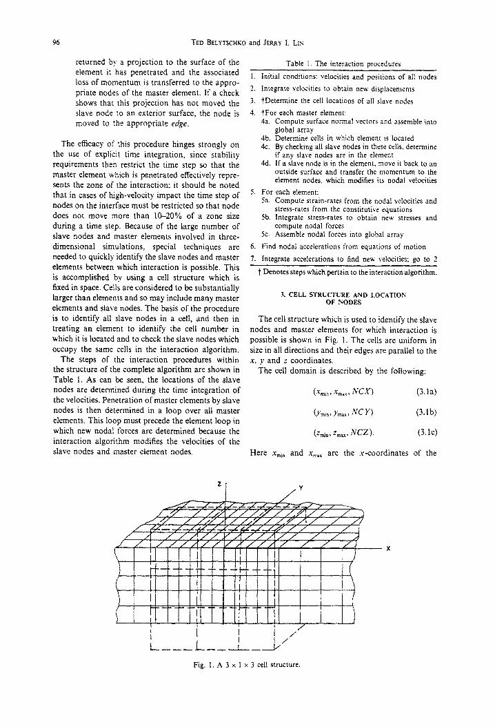
The cell structure which is used to identify the slave nodes and master elements for which interaction is possible is shown in Fig. 1. The cells are uniform in size in all directions and their edges are parallel to the X, y and z coordinates.

The ceil domain is described by the following:

(3. I a)

(3.lb)

(3. lc)

Here x,~,, and x,,,,, are the s-coordinates of the

Fig. I. A 3 x I x 3 cell structure.

A 3-D impact-penetration algorithm with erosion 91

extreme points of the cell domain and NCX is the number of cells in the x-direction; the definitions of

the terms in (3.1 b) and (3. lc) are analogous.

The cell location of a node with coordinates (x. _v,

z) is computed in two steps. First the integer cell numbers in the x, y and z directions are computed by

IX = NCX* (x - x,,)/(x,, - xc,) + 1

IY = NCY* CY - ,‘,,)/Cv,, -v,,,) + 1

(3.2a)

(3.2b)

IZ = NCZ* (z - z,,)/(z,, - zmin) + 1. (3.k)

These numbers are then used to compute the cell number of the node, ZCELL, as follows. If the node is outside the cell domain, the cell number ICELL is set to zero, i.e.

ICELL=Q if IX<1 or IX>NCX

or IYcl or IY>NCY

or IZ < 1 or IZ > NCX. (3.3)

Otherwise, ICELL is computed by

ICELL = (IZ - l)*NCX*NCY

+ (IY - l)*NCX + IX. (3.4)

The locations of all slave nodes are stored in an array K = LOCSLA(IC, J), where ZC is the cell num- ber and K is the node number of the Jth slave node in cell IC. If LOCSLA(IC, 1) = 0, then no slave nodes are located within cell IC.

The identification of the cell locations of slave nodes is made during the time integration loop. AS the new positions of slave nodes are calculated (prior to any adjustment for interaction with master ele- ments), the cell number is obtained by the procedures (3.2)-(3.4).

For purposes of efficiency, the cell structure should extend only over the domain in which interaction is

expected. This includes the domain occupied by the master elements in the undeformed configuration and any part of the domain into which master elements are anticipated to move as a result of the interaction. Although the optimal relation between cell size and master element size has to be determined, a cell should span at least two element lengths in each direction to reduce the number of elements which occupy more than one cell. A cell structure consisting of 3 x 3 x 1 cells in the .T, y and r directions as shown in Fig. 1 has been found quite effective in the

calculations performed so far.

4. ELEXIENT PENETRATION DETECTION

Any slave nodes which penetrate an element are treated during a loop through the elements; this loop is separate from the element loop in which the nodal forces are updated, and considers only master elements. The element level steps consist of the following for each element e:

(1) determine whether any slave node has pene- trated element e;

(2) if a slave node has penetrated element e, place the node outside the element and transfer the momentum loss to the element nodes.

Note that this procedure is carried out only for muster elements so the subdomain of the target that is designated to consist of master elements must be sufficiently large so that no slave node can penetrate the target without penetrating a master element.

The algorithm for step 1 must be streamlined as much as possible in order to insure that computer time is not wasted. The cell scheme is used to minim- ize as much as possible the number of computations required. The details of the procedure are as follows.

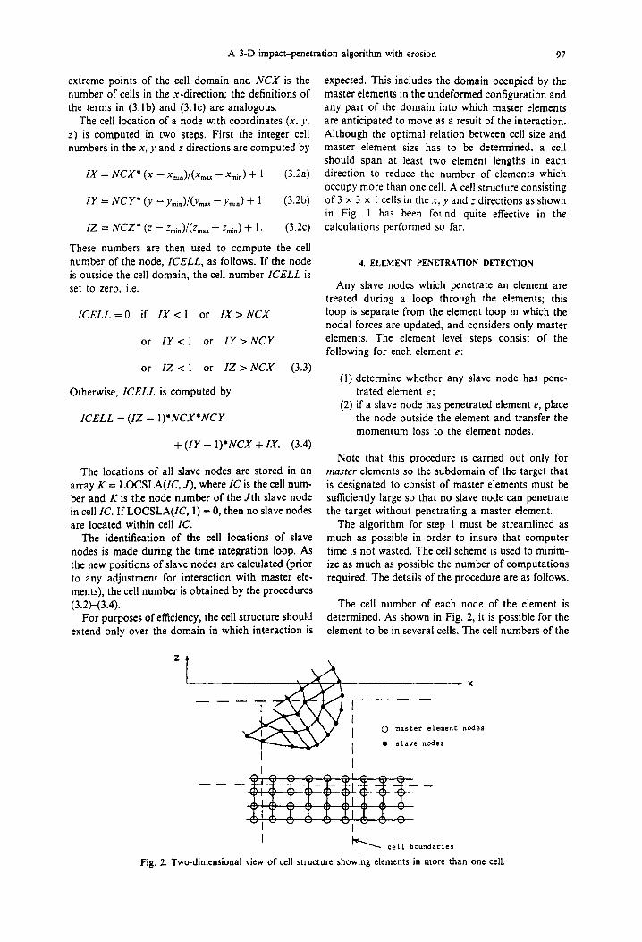
The cell number of each node of the element is determined. As shown in Fig. 2, it is possible for the element to be in several cells. The cell numbers of the

I

0 master element nodes

a slave nodes

I

cell boundaries

Fig. 2. Two-dimensional view of cell structure showing elements in more than one cell.

98 TED BELYISCHKO and JERRY I. LIN

7

6

1

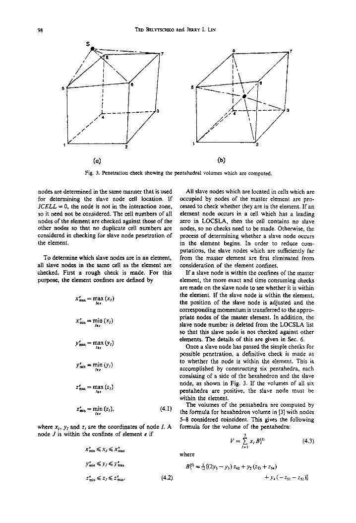
(4 (b) Fig. 3. Penetration check showing the pentahedral volumes which are computed.

nodes are determined in the same manner that is used for determining the slave node cell location. If ICELL = 0, the node is not in the interaction zone, so it need not be considered. The cell numbers of all nodes of the element are checked against those of the other nodes so that no duplicate cell numbers are considered in checking for slave node penetration of the element.

To determine which slave nodes are in an element, all slave nodes in the same cell as the element are checked. First a rough check is made. For this purpose, the element contines are defined by

G2.X = T.;x W

zc,, = m==: G%), (4.1)

where x,, yI and z, are the coordinates of node I. A node J is within the confines of element e if

All slave nodes which are located in cells which are occupied by nodes of the master element are pro- cessed to check whether they are in the element. If an element node occurs in a cell which has a leading zero in LOCSLA, then the cell contains no slave nodes, so no checks need to be made. Otherwise, the process of determining whether a slave node occurs in the element begins. In order to reduce com- putations, the slave nodes which are sufficiently far from the master element are first eliminated from consideration of the element confines.

If a slave node is within the confines of the master element, the more exact and time consuming checks are made on the slave node to see whether it is within the element. If the slave node is within the element, the position of the slave node is adjusted and the corresponding momentum is transferred to the appro- priate nodes of the master element. In addition, the slave node number is deleted from the LOCSLA list so that this slave node is not checked against other elements. The details of this are given in Sec. 6.

Once a slave node has passed the simple checks for possible penetration, a definitive check is made as to whether the node is within the element. This is accomplished by constructing six pentahedra, each consisting of a side of the hexahedron and the slave node, as shown in Fig, 3. If the volumes of all six pentahedra are positive, the slave node must be within the element.

The volumes of the pentahedra are computed by the formula for hexahedron volume in f3] with nodes 5-g considered coincident. This gives the following formula for the volume of the pentahedra:

5

V= cxrBj5’ (44.3) I-1

where

B?’ = $ WYS -Y,) 242 + ~2 @s> f zw)

zk,, Q z, c .z;,. (4.2) + Y4 (- 253 - zsdl

A 3-D impact-penetration algorithm with erosion 99

w = B KY4 - ZY,) z31+ y3 (234 + qg )

B{j’ = & KY, - 2Y,) 242 +Y4 (23, + 252)

+Yz(-% -zdl

as1 = 6 KJY, - YJ Z3f + Yl @J2 + za>

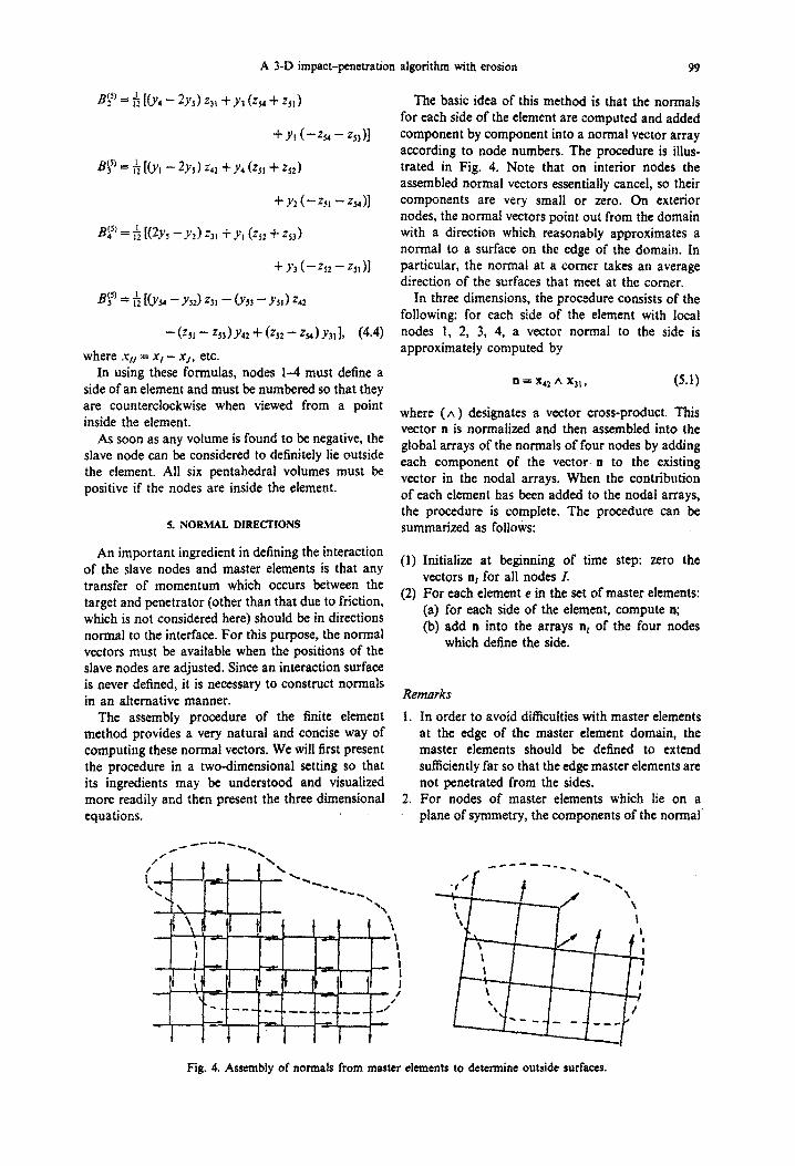
The basic idea of this method is that the normals for each side of the element are computed and added component by component into a normal vector array according to node numbers. The procedure is illus- trated in Fig. 4. Note that on interior nodes the assembled normal vectors essentially cancel, so their components are very small or zero. On exterior nodes, the normal vectors point out from the domain with a direction which reasonably approximates a normal to a surface on the edge of the domain. In particular, the normal at a comer takes an average direction of the surfaces that meet at the comer.

B$S’ = h KY34 - YJJ ZSi - C&l - Y,,) r.%,

- (rs, - 253 ) Y42 + cQ* - %I > Y3r I, (4.4)

where xN = x, - x,, etc.

In three dimensions, the procedure consists of the following: for each side of the element with local nodes 1, 2, 3, 4, a vector normal to the side is approximately computed by

In using these formulas, nodes 1-4 must define a side of an element and must be numbered so that they are counterclockwise when viewed from a point inside the element.

n=x42A~31, (5.1)

As soon as any volume is found to be negative, the slave node can be considered to definitely lie outside the element. All six pentahedral volumes must be positive if the nodes are inside the element.

5. NORMAL DIRECTIONS

where (A) designates a vector cross-product. This vector n is normalized and then assembled into the global arrays of the normals of four nodes by adding each component of the vector n to the existing vector in the nodal arrays. When the contribution of each element has been added to the nodal arrays, the procedure is complete. The procedure can be summarized as follows:

An important ingredient in defining the interaction of the slave nodes and master elements is that any transfer of momentum which occurs between the target and penetrator (other than that due to friction, which is not considered here) should be in directions normal to the interface. For this purpose, the normal vectors must be available when the positions of the slave nodes are adjusted. Since an interaction surface is never defined, it is necessary to construct normals in an alternative manner.

(1) Initialize at beginning of time step: zero the vectors n, for all nodes i.

{2) For each element e in the set of master elements: (a> for each side of the element, compute a; (b) add II into the arrays nI of the four nodes

which define the side.

Remarks

The assembly procedure of the finite element 1. In order to avoid difficulties with master elements method provides a very natural and concise way of at the edge of the master element domain, the computing these normal vectors. We will first present master elements should be defined to extend the procedure in a two-dimensional setting so that sufficiently far so that the edge master elements are its ingredients may be understood and visualized not penetrated from the sides. more readily and then present the three dimensional 2. For nodes of master elements which lie on a equations. plane of symmetry, the components of the normal

Fig. 4. Assnnbly of normals from master elements to determine outside surfaces.

100 TED BELYTXHKO and JEICRY 1. IS

vector which do not lie in the plane of symmetry are set to zero.

3. For master elements which lie on the bottom of the target (opposite to the original position of the projectile), the normals to the bottom surface are omitted to avoid driving the slave nodes in the wrong direction.

6. ADJUSTMENT OF SLAVE NODE POSITIONS

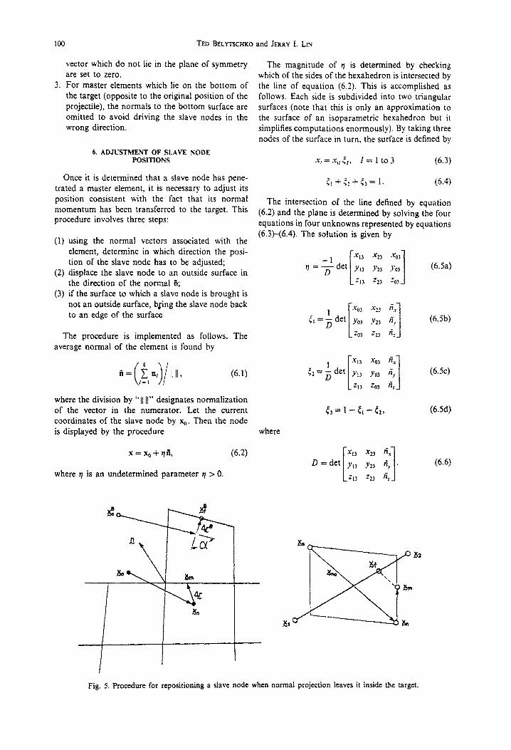
Once it is determined that a slave node has pene- trated a master element, it is necessary to adjust its position consistent with the fact that its normal momentum has been transferred to the target. This procedure involves three steps:

(1) using the normal vectors associated with the element, determine in which direction the posi- tion of the slave node has to be adjusted;

(2) displace the slave node to an outside surface in the direction of the normal 8;

(3) if the surface to which a slave node is brought is not an outside surface, bfing the slave node back to an edge of the surface

The procedure is implemented as follows. The average normal of the element is found by

fi= f: nI II II, ( Ii I-1 (6.1)

where the division by ” 1) /I” designates normalization of the vector in the numerator. Let the current coordinates of the slave node by x0. Then the node is displayed by the procedure

x=x,+‘lii, (6.2)

where q is an undetermined parameter q > 0.

The magnitude of r~ is determined by checking which of the sides of the hexahedron is intersected by the line of equation (6.2). This is accomplished as follows. Each side is subdivided into two triangular surfaces (note that this is only an approximation to the surface of an isoparametric hexahedron but it simplifies computations enormously). By taking three nodes of the surface in turn, the surface is defined by

.r, = .Y{[ &, I=1to3 (6.3)

<I f & + 5s = 1. (6,4)

The intersection of the line defined by equation (6.2) and the plane is determined by solving the four equations in four unknowns represented by equations (6.3X6.4). The solution is given by

-1 q =% det

where

r2 =i det Xl3 x01 4

i -1

Y13 Yo3 f."

213 zo3 fi:

c3= 1 -t,- (29

(6Sa)

(6Sb)

(6.5~)

(6Sd)

(6.6)

Fig. 5. Procedure for re~sitioning a slave node when normal projection leaves it inside the target.

A 3-D impact-~netration algorithm with erosion 101

A particular triangular surface is intersected by the parametric ray of equation (6.2) if and only if

r1>0 (6.7)

O<&<l. for I=1 to3. (6.8)

Once the surface on which the slave node is projected is determined, the surface is checked to ascertain whether it is an outside surface, This is done by checking whether the four normals of the nodes of the surface are non-zero. If this check fails, the node is projected to an edge of the surface as shown in Fig. 5.

The equations which govern this realignment of the slave node are the following. Let x, be given by

~,=x,+Atv”‘~, (6.9)

where x, is the position of the slave node at the beginning of the time step as shown in Fig. 5. The edges of the side are then considered in turn and its nodes are genericalfy identified as 1 and 2, with the vector connecting them denoted by x2,. The previ- ously computed new position of the node is denoted by x,, where

x, = x, + Ar. (6.10)

The node is then repositioned on the intersection of the line x1* with the plane defined by the vectors x, and x,,. The equations to be solved are

Xl0 + xzi Vi - %!I ‘12 - %ln tf3 - - 0, (6.11)

where Q, i L- t to 3, are the unknowns. If the edge x1, is the correct one q, must satisfy 0 < 9, < 1. Other- wise, another edge of the surface is considered.

The final position is denoted by xr which is given

by

x/= XI + 91 x21, (6.12a)

where q, is the above solution. The reposition vector is then redefined by

Ar=xi,=xf-xn. (6.12b)

If a slave node is on a plane of symmetry, the component or Ar normal to the plane of symmetry is now set to zero.

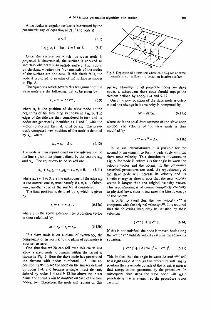
One situation which can foil even this check and allow a slave node to remain within the target is shown in Fig. 6. Here the slave node has penetrated the element with nodes numbered l-g. The re- positioning will place the node on the surface defined by nodes I-4, and because a single intact element, defined by nodes l-4 and 9-12 Iies above the intact plane, the normals wilf be nonzero on each of the four nodes, l-4. Therefore, the node will remain on this

Fig. 6. Depiction of a situation where checking for nonzero normals is not sutlicient to detect an interior surface.

surface. However, if all projectile nodes are slave nodes, a subsequent slave node should engage the element defined by nodes l-4 and 9-12.

Once the new position of the slave node is deter- mined the change in its velocity is computed by

Av = Air/At, (6.13a)

where Ar is the total displacement of the slave node needed. The velocity of the slave node is then modified by

v”W = void + Av. (6.13b)

In unusual circumstances it is possible for the normal of an element to form a wide angle with the slave node velocity. This situation is illustrated in Fig. 5, for node B, where a is the angle between the velocity vector and the normal. If the previously described procedures are used, the repositioning of the slave node will increase its velocity and its kinetic energy as shown; note that the new velocity vector is longer than the original velocity vector. This repositioning is of course completely contrary to physical laws, since it increases the kinetic energy of the system.

In order to avoid this, the new velocity Pew is compared with the original velocity void. It is required that the following inequality be satisfied by these velocities:

j/ Pew 11 < /I void I/ . (6.14)

If this is not satisfied, the node is moved back along the vector v~‘” until its velocity satisfies the foliowing equation:

/I vnew I/‘+ )( A r/At II2 = 11 void /I’. (6.15)

This implies that the angle between Ar and vnW will be a right angle. Although this procedure will usually position the slave node outside of the target, it insures that energy is not generated by the procedure. In subsequent time steps the slave node will again penetrate a master element so the procedure is not ha~fu1.

102 TED BEI_WCHKO and JERRY 1. LIS

The momentum loss associated with this adjust- ment is MAv, where M is the mass of the slave node. This momentum is now transferred to the nodes of the penetrated surface. The formula used for node J of the surface is

Av ,=-$n~fiAv (no sum on JX (6.16) I

where m, is its mass and

(6.17)

This formula apportions the momentum to the nodes according to how strongly their vectors point in the direction of the interface normal ii.

Table 2. Parameters for Example I

Projecrile Shape Dimensions Density Bulk modulus Shear modulus Yield stress Ultimate stress Initial velocity

Targer Shape Dimensions Density Bulk modulus Shear modulus Yield stress Ultimate stress initial velocitv

rod with a round nose 4.04 in. long, 0.201 in. radius OOOO73 lb-sec’iin’ 23.810,~0 psi I 1,630,OOO psi 250,oOO psi 310,OOO psi .x-component 56155.0 inisec z-component - 3242 I .O inisec

plate 5.6 in. x 0.6 in. x I in. (half piate) OOOO73 lb-sec’jin“ 27,780,OOO psi 11,360,OOO psi I60,OOO psi 185,000 psi 0

7. NUMERICAL EXAMPLES

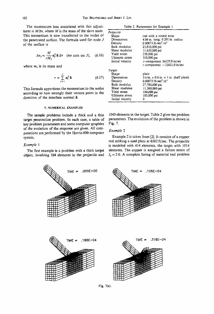
The sample problems include a thick and a thin target penetration problem. In each case, a table of key problem parameters and some computer graphics of the evolution of the response are given. All com- putations are performed by the Harris-800 computer system.

Example t

The first example is a problem with a thick target object, involving 104 elements in the projectile and

1040 elements in the target. Table 2 gives the problem parameters. The evolution of the problem is shown in Fig. 7.

Example 2

Example 2 is taken from [2]. It consists of a copper rod striking a steel plate at 6562 ftjsec. The projectile is modeled with 414 elements, the target with 1014 elements. The copper is assigned a failure strain of 5 = 2.0. A complete listing of material and problem

TIME = .318E-04

Fig. 7(a).

A 3-D impact-penetration algorithm with erosion

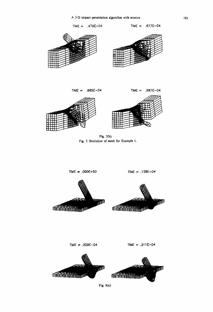
TIME = .479E-04 TIME = .W?E-04

103

TIME = .88X-04 TIME = .987E-04

Fig. 7(b).

Fig. 7. Evolution of mesh for Example 1.

TIME = .OOOE+OO TIME = .I 28E-04

TIME = .229E-04 TIME = ,311 E-04

Fig. 8(a).

I04 TED BELYTSCHKO and JERRY I. l.,r~

TlME = .366E-34 TIME = .405E-04

TiME = ,453E-04 TIME = .48X-04

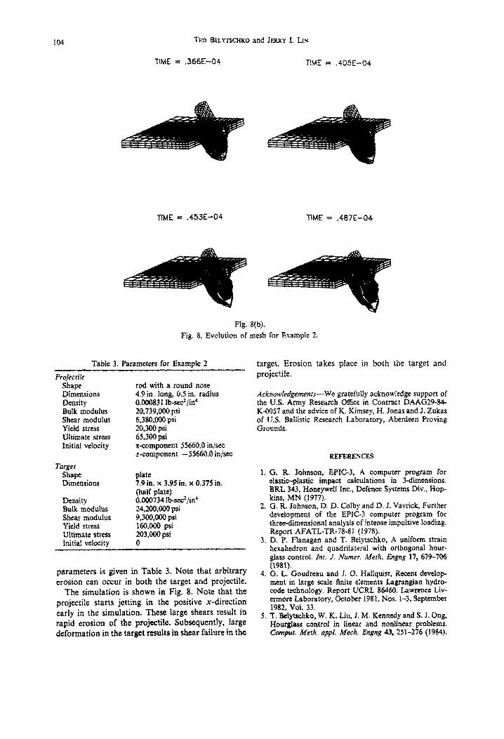
Fig, Sfb). Fig. 8. Evolution of mesh for Example 2.

Table 3. Parameters for Example 2

Projecrite Shape Dimensions Density Bulk modulus Shear modulus Yield stress ~~t~rn&t~ &es5 Initial velocity

Target Shape Dimensions

Density Bulk modulus Shear modulus Yield stress tiltimate stress Initial velocity

rod with a round nose 4.9 in. kng, 0.5 in. radius ~.~831 lb-sec’/in’ 20,739,080 psi 6,380,OOO psi 20.309 usi

paraneters is given in Table 3. Note that ~~b~~~~~ erosion can occur in both the target and projectik,

The ~rn~~a~~~~ is shown in Fig, 8. IWe that the projectile starts jetting in the positive x-direction early in the simulation. These large shears result in rapid erosion of the projectiil. ~ub~~ue~~I~, brge deformation in the targot nsuits in shear failure in the

target Erosion takes place in both the target and projectile.

~~k~aw~e~g~~~~~$-We gratefully acknowledp support of the US. Army Research Office in Contract DAAtr29-84 K-0057 and the advice of K. Kimsey, II. Jonas and J. Zukas of U.S. Ballistic Research Laboratory, Aberdeen Proving Grounds.

I. G. R. Johnson, EPIC-3, A computer program for &&tic-plastic impact calculations in 3-dimensions. BRL 343, Honeywell Inc., Defence Systems Div., Rap kins, MN (1977).

2. G, R. Johnson, IX D. Coiby and D. f. Vavrick, Further development of the EPIC3 computer program for three-dimeusjonai analysis of intense impulsive loading. Report AFAT~-TR-78.gI (1978).

3. D. P. Flanagan and T. Belytscbko, A uniform strain hexahedron and quadrilateral with orthogonal hour- glass controf. inr. J. Nwrer. Merh. Engng 17, 679-706 (19813.

4. 6. L. Goudreau and J. 0, Hallquist, Recent develop- ment in large scale finite elements Lagrangian hydro- code technofogy. Report UCRL 86460. Lawrence Liv- et-more Laboratory, October 198f, Nos. l-3, September t982, Vol. 33.

5. T. Beiytschko, W. K. Liu, J. M. Kennedy and S. 1. Ong, ~~u~~ control in linear and downer problems. Cwsqxa Me&. appi! Me&. Engrzg 43, 251-276 (1984).