A variational principle for molecular motors

MICHEL CHIPOT, DAVID KINDERLEHRER, AND MICHAL KOWALCZYK

Dedicated to PIERO VILLAGGIO

1. Introduction

Intracellular transport in eukarya is attributed to motor proteins that transduce chemical

energy into directed mechanical motion. Muscle myosin has been known since the mid

nineteenth century and its role in muscle contraction demonstrated by A. F. Huxley and

H. E. Huxley in the 1950's. Kinesins and their role in intracellular transport were

discovered only in 1985, [20]. These nanoscale sized motors carry organelles and other

cargo on microtubules. They function in a highly viscous setting with overdamped

dynamics. Taken as a system, they are in configurations far from conventional notions of

equilibrium even though they are in an isothermal environment. Because of the presence

of significant diffusion in the environment they are sometimes referred to as Brownian

motors. Since a specific type tends to move in a single direction, for example, either

anterograde or retrograde to the cell periphery, these proteins are sometimes referred to as

molecular rachets.

In this note we establish a dissipation principle that describes transport in a typical motor

system like conventional kinesin. This begins a chain of events. It suggests, in a natural

way, a variational principle and an implicit scheme in the sense of Otto [14], [15] and

Jordan, Kinderlehrer and Otto [10]. This determines, in turn, a system of differential

equations, by design that suggested by Adjari and Prost, cf. [16], or by Doering,

Ermentrout, and Peskin [4] and Peskin, Ermentrout, and Oster [17]. We have a clear

notion of equilibrium or minimum energy for a macroscopic process. However, to quote

J. L. Ericksen, a great friend of Prof. Villaggio, most of the systems we meet are only

metastable. It is, indeed, very common to model systems in a way that this metastability

disappears. Moreover even when we permit this type of behavior, when we think of

evolution, especially when we have in hand a smooth solution, we often neglect to

recognize that in saying states are close to each other we are imposing an environment for

2

the motion. The novelty of our principle is that it sets this dynamical environment for the

process in a weak topology as described by a Kantorovich-Wasserstein metric. This

owes in part to a result of Benamou and Brenier [2]. Our derivation illustrates the

feasibility of mesoscale modeling for these systems.

In [11] we discussed a different type of model, the flashing rachet, cf. Astumian [1].

Here we were successful in approximating the system by a Markov chain on Dirac

masses and were able to show how this led to transport in the system.

The version of these descriptions that we consider is a two state model consisting of a

system of Fokker-Planck Equations coupled by first order chemistry. For this, we take

Ω = (0,1) and

σ > 0 constant

ψi ≥ 0 and νi ≥ 0, i = 1,2, smooth and periodic of period X = 1/M

with supp ν1 = supp ν2 and ν1 + ν2 ≤ 1.

M is an integer. We often abbreviate writing bi = i'ψ .

We ask for ρ = (ρ1, ρ2) satisfying

∂

∂1ρ

t =

∂∂x

(σ∂

∂1ρ

x + b1ρ1) – ν1 ρ1 + ν2 ρ2

in Ω, t > 0∂

∂2ρ

t =

∂∂x

(σ∂

∂2ρ

x + b2ρ2) + ν1 ρ1 – ν2 ρ2

(1.1)

σ∂

∂1ρ

x + b1ρ1 = 0

on ∂Ω, t > 0

σ∂

∂2ρ

x + b2ρ2 = 0

ρ1 = 10( )ρ and ρ2 = 2

0( )ρ in Ω, t = 0.

3

We assume that

10( )ρ ≥ 0, 2

0( )ρ ≥ 0, and ∫Ω

( 10( )ρ + 2

0( )ρ ) dx = 1. (1.2)

Explanations of these equations may be found in [4], [16], [17], cf. also [19]. We give

our derivation in §4. It is a classical fact that under (1.2) solutions of the system (1.1)

are nonnegative [18] and, thanks to the boundary condition,

∫Ω

(ρ1 + ρ2) dx = 1 for all t.

Fig. 1 A typical ψ1.

Fig. 2 A typical ψ2. Note that the minima of ψ2 interpolate the minima of ψ1.

The key elements to achieve transport are

(a) asymmetry of the potentials ψi in a given period interval and

(b) the relationship of the conformation change factors νi to the ψi .

ψ1

ψ2

4

Here we provide results of simulations to illustrate this, leaving to a future work the

analysis. Prior to proceeding, we would like to remark on a few aspects of (1.1).

Fig. 3 Typical conformational change coefficient ν1 = ν2 . Note that the maxima ofνi are located at the minima of the potentials.

(i) νi constant. Suppose that the νi ≥ 0 with ν1 + ν2 = 1 are constants.

For the moment denote by

µi(t) = ∫Ω ρi(x,t) dx (1.3)

so µ1 + µ2 = 1. Then, using the boundary condition, we have a system of ordinary

differential equations

d

dt

µ1 = –ν1 µ1 + ν2 µ2 and d

dt

µ2 = ν1 µ1 – ν2 µ2 (1.4)

and thus

µ(t) = (ν2,ν1) + c e–t(1,–1) → (ν2,ν1) (1.5)

exponentially fast. Hence although the averages are not a good indicator of distance to

equilibrium for the system, they do converge rapidly. For these averages we also have

that their entropy is decreasing, namely,

νi

5

d

dt(µ1 log µ1 + µ2 log µ2) < 0. (1.6)

(ii) comparison with ordinary Fokker-Planck Equation. Consider briefly the

problem

∂∂ρt

= ∂∂x

(σ∂∂ρx

+ bρ) in Ω, t > 0

σ∂∂ρx

+ bρ = 0 on ∂Ω, t > 0 (1.7)

ρ = ρ0 in Ω, t = 0.

where ρ0 ≥ 0 and ∫Ω ρ0 dx = 1. Above b = ψ ', where ψ ≥ 0 is a smooth

potential. Let

ρ#(x) = 1Z

– ( )ψσ

x

e , Z = ∫Ω

– ( )ψσ

x

e dx , (1.8)

denote the stationary solution of (1.7). It is a standard computation that

d

dt σ ∫

Ω ρ log

ρ

ρ# dx =

d

dt ∫

Ω (ψ ρ + σ ρ log ρ) dx

= – ∫Ω

1ρ

(σ∂∂ρx

+ bρ)2 dx < 0,

from which it follows that

∫Ω

ρ log ρ

ρ# dx → 0 as t → ∞.

6

Since, by the Cesar - Kullback Inequality, just based on the fact that t log t is convex,

[13] p. 15,

( ∫Ω

| ρ(x,t) – ρ#(x)| dx )2

≤ 2 ∫Ω

ρ log ρ

ρ# dx,

the decrease of the entropy implies that the solution

ρ(x,t) → ρ#(x) in L1(Ω) as t → ∞.

Consequently both in cases (i) and (ii) above, an entropy inequality is a key to the trend

to equilibrium. We shall show this again, in a different context, for (1.7), but we are

unable to determine such behavior in such a straightforward manner for our system (1.1).

In fact, it is not even obvious that there is a stationary solution to (1.1); however a proof

may be based on the Schauder Fixed Point Theorem.

2. Resumé of transport

In this section we give a brief description of the Kantorovich-Wasserstein metric and its

relationship to transport, eg. [6]. Given densities f, f* ∈ L1(Ω) with

∫Ω

f dx = ∫Ω

f* dx = c > 0,

suppose that there is a strictly increasing continuous mapping

φ : Ω → Ω, φ(0) = 0, φ(1) = 1,

such that

∫Ω ζ

f dx = ∫

Ω ζ(φ(x))

f*(x) dx for ζ ∈ C(Ω). (2.1)

7

We then say that f is the push forward of f* and φ is the associated transfer function.

In particular, if ζ = χA, the characteristic function of A ⊂ Ω, then

∫A

f(x) dx = ∫φ–1(A)

f*(x) dx,

or with E = φ–1(A),

∫φ(E)

f(x) dx = ∫ E

f*(x) dx.

In particular for E = [0, x],

∫[0,φ(x)]

f(x') dx' = ∫ [0.x]

f*(x') dx',

or

F(φ(x)) = F*(x),

where F and F* are the distribution functions of f and f*. Thus, in one dimension, the

transfer function is uniquely determined as

φ(x) = F–1(F*(x)), x ∈ Ω, (2.2)

which was known to Frechet, [5].

Now φ is the unique solution of the Kantorovich formulation of the Monge-Kantorovich

mass transfer problem: among all joint distributions q(x,y) with marginals f and f*.

d(f, f*)2 = min ∫Ω×Ω

| x – y |2 dq(x,y) = ∫Ω

| x – φ(x) |2 f*(x) dx.(2.3)

| x – y |2 may be replaced by any suitable cost function in this one-dimensional situation.

It turns out that d is a metric on the measures f dx with mass c which induces the

weak* topology on them (as the dual space of C(Ω)).

8

Now suppose that f(x,t), 0 ≤ t ≤ τ, and f*(x) are given with

∫Ω

f(x,t) dx = ∫Ω

f* dx = c > 0 with transfer functions φ(x,t).

Thus,

∫Ω ζ(x)

f(x,t) dx = ∫

Ω ζ(φ(x,t))

f*(x) dx for ζ ∈ C(Ω), 0 ≤ t ≤ τ, (2.4)

and in particular,

∫[0,φ(x,t)]

f(x') dx' = ∫ [0.x]

f*(x') dx'.¸

Assuming requisite smoothness, differentiate this expression with respect to x and t.

Then

f(φ(x,t),t) ∂φ∂x

= f*(x) and

fξ(φ(x,t),t) ∂φ∂t

∂φ∂x

+ ft(φ(x,t),t) ∂φ∂x

+ f(φ(x,t),t)2∂

∂ ∂φ

x t = 0.

Now define a velocity by

∂φ∂t

= v(φ, t) so 2∂

∂ ∂φ

x t = vξ (φ, t)

∂φ∂x

.

Substituting gives

ft + (v f)x = 0 in Ω, 0 < t < τ. (2.5)

9

So f is the solution to a continuity equation. The converse is easy to check. Brenier and

Benamou [2] show that

d(f**,f*)2 = τ v

min ∫0

τ

∫

Ω v2 f dx dt, (2.6)

where

ft + (v f)x = 0 in Ω, 0 < t < τ,

f(x,0) = f*(x), f(x,τ) = f**(x). (2.7)

We review their verification of this. Let φ denote the transfer function for f**, f*.

Given f(x,t) satisfying (2.7), by (2.4),

∫Ω

v(ξ,t)2 f(ξ,t) dξ = ∫Ω

v(φ(x,t),t)2 f*(x) dx and

τ ∫0

τ

∫Ω

v(ξ,t)2 f(ξ,t) dξ dt = τ ∫0

τ

∫Ω

v(φ(x,t),t)2 f*(x) dx dt

= τ ∫0

τ

∫Ω φt(x,t)2 f*(x) dx dt.

On the other hand, recalling that φ(x,0) = x, by Schwarz's Inequality,

| x – φ(x,τ)| = | φ(x,0) – φ(x,τ)| ≤ ∫0

τ | φt(x,t) | dt

≤ τ (∫0

τ φt(x,t)2 dt )

1/2

.

Multiplying by f* and integrating gives

d(f**,f*)2 = ∫Ω

| x – φ(x,τ)|2 f*(x) dx ≤ τ ∫0

τ ∫

Ω φt(x,t)2 f*(x) dx dt (2.8)

10

= τ ∫0

τ ∫

Ω v(ξ,t)2 f(ξ,t) dξ dt.

Thus

d(f**,f*)2 ≤ inf τ ∫0

τ ∫

Ω v(ξ,t)2 f(ξ,t) dξ dt.

Now choose the special φ(x,t) = x + t

τ ( φ (x) – x). For this choice,

φt(x,t) = 1τ

( φ (x) – x),

and equality holds in (2.8). This shows (2.6).

3. Dissipation and the Kantorovich-Wasserstein metric

In this section, we discuss a dissipation inequality and use it to suggest a variational

principle for a general Fokker-Planck Equation. To begin, we establish an expression for

the dissipation in an ensemble of mass-spring-dashpot systems. For a single elementary

mass-spring-dashpot system, we commonly write an ordinary differential equation

m 2

2d

dt

ξ + γ

d

dt

ξ + κ ξ = F, 0 < t < τ

ξ(0) = x (3.1)d

dt

ξ(0) = 0

Multiplying by d

dt

ξ and integrating over (0, τ) gives the familiar relation

12 m

d

dt

ξ(τ)2 + γ ∫

0

τ( d

dt

ξ )

2

dt + κ2

ξ(τ)2 = κ2

x2 + F(ξ(τ) – x), (3.2)

11

relating the kinetic energy, the potential energy, the work done on the system, and the

energy loss due to frictional dissipation. In particular,

γ ∫0

τ( d

dt

ξ )

2

dt

is the term which represents the dissipation. We may regard τ as a relaxation time. Our

interest is in the left hand side of (3.2). Suppose an ensemble is distributed with a

number density f*(x). Set ξ = φ(x,t). Then at time τ we have for this ensemble

12 m ∫

Ω φt (x,τ)2 f*(x) dx + γ ∫

0

τ ∫

Ω φt(x,t)2 f*(x) dx dt +

κ2

∫Ω φ(x,τ)2 f*(x) dx

which identifies

δ = γ ∫0

τ ∫

Ω φt(x,t)2 f*(x) dx dt (3.3)

as the energy dissipated in the system. Define the transported density f(ξ,t) by

∫Ω ζ(ξ) f(ξ,t) dx = ∫

Ω ζ(φ(x,t)) f*(x) dx, 0 ≤ t ≤ τ (3.4)

so we have that

δ = γ ∫0

τ ∫

Ω v(ξ,t)2 f(ξ,t) dx dt with (3.5)

ft + (v f)ξ = 0 in Ω, 0 < t < τ,

analogous to the discussion of the last section. For a fixed initial distribution f* and

terminal distribution f(x) = f(x,τ),

12

min ∫0

τ ∫

Ω v(ξ,t)2 f(ξ,t) dx dt =

1τ

d(f, f*)2, (3.6)

where d is the Kantorovich-Wasserstein distance.

The above permits us to write the dissipation inequality for successive states of the

system as an implicit scheme. First recall that our system is overdamped and kinetic

energy may be ignored, as discussed in the introduction. Suppose that we are given a

potential ψ ≥ 0 and a diffusion coefficient σ. Take γ = 12 for simplicity. Assume

that the system starts from a distribution f* and relaxes to a distribution f during a

relaxation time τ. Then we require that

12 ∫

0

τ ∫

Ω v(ξ,t)2 f(ξ,t) dx dt + ∫

Ω ψ(ξ) f(ξ) + σ f(ξ) log f(ξ) dξ ≤

∫Ω

ψ(ξ) f*(ξ) + σ f*(ξ) log f*(ξ) dξ (3.7)

whenever

ft + (v f)ξ = 0 in Ω, 0 < t < τ,

f(x,0) = f*(x), f(x,τ) = f(x). (3.8)

So,

12τ

d(f, f*)2 + ∫Ω

ψ(ξ) f(ξ) + σ f(ξ) log f(ξ) dξ ≤

∫Ω

ψ(ξ) f*(ξ) + σ f*(ξ) log f*(ξ) dξ (3.9)

Our dissipation principle is: given a probability density f* ≥ 0, find a probability

density f such that

13

12τ

d(f, f*)2 + ∫Ω

ψ f + σ f log f dx = min. (3.10)

Since f* is among the admissible competitors in (3.10) and d(f*, f*) = 0, (3.9) is

automatically satisfied when f satisfies (3.10).

We take a moment to interpret (3.10) as an implicit scheme, [10]. With f (0) given, and

f (1), …, f (k–1) known, determine f (k) by solving (3.10) with f* = f (k–1) and lable the

solution f(k). Define

f (τ)(x,t) = f (k)(x) for kτ ≤ t < (k + 1)τ. (3.11)

In [10], it is shown that f (τ) → f as τ → 0 and f is a solution of the Fokker-Planck

Equation

∂∂f

t = σ

2

2∂∂

f

x +

∂∂x

(ψ' f) in Ω, t > 0

σ ∂∂f

x + ψ' f = 0 on ∂Ω, t > 0 (3.12)

f = f (0) in Ω, t = 0

4. A variational principle for a molecular motor

Let us discuss the hand-over-hand (rotating cross-bridge) model for conventional kinesin,

[8]. Conventional kinesin has two identical head domains (heavy chains) which walk in a

hand over hand fashion along a rigid microtubule. A head may be thought of as having

two states: an a state when it undergoes conformational change owing to release of ADP

and binding of ATP and a b state executing a powerstroke when it steps along the

microtubule, releasing Pi. The a state for head 1 induces the b state for head 2. We

regard the a state conformational change to be governed by a first order chemistry

description and the b state by interaction with potentials, diffusion, and dissipation.

14

Divide the heads of the ensemble of motors into two sets, set 1 and set 2; for example the

set 1 motors attach to the odd-labeled sites on microtubules and the set 2 motors attach to

even labled sites. This permits distance along the microtubule to be used as a process

variable. Let ρ1 and ρ2 denote the relative densities of set 1 and set 2 motors in state b,

the powerstroke state. Introduce, the the standard way, the potentials and coefficients for

conformational change

σ > 0 constant

ψi ≥ 0 and νi ≥ 0, i = 1,2, smooth and periodic of period X = 1/M

with supp ν1 = supp ν2 and ν1 + ν2 ≤ 1. (4.1)

Let

ν = 1 1

2 2

–

–

ν ν

ν ν

and P = 1 + τ ν, (4.2)

where τ is a relaxation time. In view of the discussion above, set 1 heads enter the a

state at the rate that set 2 heads enter the b state and vice versa. We may thus envision a

cycle, starting with a density ρ* = ( 1*ρ , 2

*ρ )

ρ∗ → ρ∗ P → ρ (4.3)

subject to the dissipation principle: given ρ∗ , such that

∫Ω

( 1*ρ + 2

*ρ ) dx = 1 and i*ρ ≥ 0 in Ω,

determine ρ by

∑i = 1,2

12τ

d(ρi, (ρ*P)i)2 + ∑

i = 1,2 ∫

Ω ψ i ρ i + σ ρ i log ρi dx = min. (4.4)

among all ρ satisfying

15

∫Ω ρ i dx = ∫

Ω (ρ∗P) i dx, and ρi ≥ 0 in Ω, i = 1,2.

This variational principle leads to (1.1). In reprise, looking at the cycle (4.3) and the

dissipation inequality (4.4), we realize that there are many systems that can be described

in a very similar fashion. Moreover, (4.4) is not unique in leading to (1.1).

Note that for τ small and ν constant, P is a probability matrix and ρ∗ → ρ∗ P is

one step in a Markov chain.

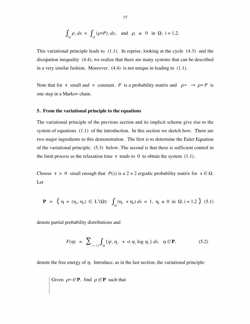
5. From the variational principle to the equations

The variational principle of the previous section and its implicit scheme give rise to the

system of equations (1.1) of the introduction. In this section we sketch how. There are

two major ingredients to this demonstration. The first is to determine the Euler Equation

of the variational principle, (5.3) below. The second is that there is sufficient control in

the limit process as the relaxation time τ tends to 0 to obtain the system (1.1).

Choose τ > 0 small enough that P(x) is a 2 × 2 ergodic probability matrix for x ∈ Ω.

Let

P = η = (η1, η2) ∈ L1(Ω): ∫Ω

(η1 + η2) dx = 1, ηi ≥ 0 in Ω, i = 1,2 (5.1)

denote partial probability distributions and

F(η) = ∑ i = 1,2

∫Ω

ψ i η i + σ η i log ηi dx, η ∈ P, (5.2)

denote the free energy of η. Introduce, as in the last section, the variational principle:

Given ρ∗ ∈ P, find ρ ∈ P such that

16

∑i = 1,2

12τ

d(ρi, (ρ*P)i)2 + F(ρ) = min P (5.31)

subject to

∫Ω ρ dx = ∫

Ω ρ∗ P dx . (5.32)

(5.32) is a vector equation. Our implicit scheme, suggested in §3, is defined by choosing

ρ(0) ∈ P and determining ρ(k) as the solution of (5.3) with ρ* = ρ(k–1). We then set

ρ (τ)(x,t) = ρ (k)(x) for k τ ≤ t ≤ (k + 1) τ (5.4)

Our objective is to show that ρ (τ) converges to the solution of (1.1).

Suppose for a moment that νi ≥ 0 are constant, ν1 + ν2 = 1. Then the averages

α(k) = ∫Ω ρ(k) dx

satisfy

α(k) = α(k–1)P (5.5)

and are iterates of a Markov Chain. As mentioned above, this is analogous to (1.4) for

the system (1.1). Hence the single statistic of the process

α(k) → α(k)P

satsifies

α(k) → α# = (ν2, ν1)

its equilibrium value, exponentially fast. The system itself may be very far from

equilibrium.

It is straightforward to check that (5.3) admists a solution since the functional F is

convex, superlinear, and bounded below. The novel feature of this variational principle is

17

that we cannot control F(ρ) in terms of F(ρ∗), and, indeed, the sequence F(ρ(k)) need

not be decreasing. The control we have is given by the elementary fact about Markov

chains that a step in the chain reduces relative entropy. More precisely, abusing our

notation for a moment:

Let P = ( pij ), pij > 0, be a probability matrix with stationary distribution µ#.

Then

∑ (µP)j log j

j

P( )#

µ

µ ≤ ∑ µj log j

j

µ

µ#(5.6)

for µj ≥ 0 (µ does not have to be a probability vector)

Now observe that η = ρ*P is admissible in (5.3) and, of course, d((ρ*P)i, (ρ*P)i) = 0.

Hence,

∑i = 1,2

12τ

d(ρi, (ρ*P)i)2 + F(ρ) ≤ F(ρ*P) (5.7)

Let µ#(x) denote the stationary distribution of P(x), whence by (5.6),

∑ i = 1,2

∫Ω (ρ∗P)i log i

i

P( )*

#

ρ

µ dx ≤ ∑

i = 1,2 ∫

Ω i

*ρ log i

i

*

#

ρ

µ dx (5.8)

So

F(ρ*P) = ∑ i = 1,2

∫Ω (ψ i + σ log i

#µ )(ρ*P) i + σ (ρ∗P)i log i

i

P( )*

#

ρ

µ dx

≤ ∑ i = 1,2

∫Ω (ψ i + σ log i

#µ )(ρ*P) i + σ i*ρ log i

i

*

#

ρ

µ dx

= F(ρ*) + τ ∑ i = 1,2

∫Ω

(ψ i + σ log i#µ )(ρ*ν) i dx.

18

Thus we arrive at our main control estimate

∑i = 1,2

12τ

d(ρi, (ρ*P)i)2 + F(ρ) ≤ F(ρ*) + τ ∑

i = 1,2 ∫

Ω (ψ i + σ log i

#µ )(ρ*ν) i dx.

(5.9)

Note that the second term is bounded by C τ since all of ψ i , i#µ , and ν are bounded

and ρ* is bounded in L1.

Now we describe the approximate Euler Equation of (5.3), whose derivation is based on

the classical method of variation of domain. Details of this will be presented elsewhere,

but cf. [3],[9], [10],[12],[14],[15]. Let ρ denote the solution of the variational principle

(5.3) for a given ρ*. Then

| ∑ i = 1,2

∫Ω

( 1τ (ρi – i

*ρ ) – (ρ* ν)i) ζi – σ i"ζ ρi + i

'ψ ρi i'ζ dx |

≤ 12 max sup | i

"ζ | 1τ ∑

i = 1,2 d(ρi, (ρ*P)i)

2 (5.10)

≤ 12 max sup | i

"ζ | (F(ρ∗) – F(ρ) + C τ) (5.11)

for ζ = (ζ1, ζ2) ∈ 0∞C (Ω)

where we have used the main estimate (5.9) in (5.11).

Suppose that T = n τ and that ρ (k) denote the solutions of the iterative scheme.

Summing (5.16), we arrive at the estimate

19

| ∑ i = 1,n

∑ i = 1,2

∫Ω

( 1τ ( i

k( )ρ – ik( – )1ρ ) –

(ρ (k–1) ν)i) ζi – σ i"ζ i

k( )ρ + i'ψ i

k( )ρ i'ζ dx τ |

≤ C0 τ (F(ρ (n)) – F(ρ (0)) + C T) (5.12)

This leads to convergence of the sequence ρ (τ) defined in (5.4)

6. Some results of simulations

In this section we present a brief summary of the results of some simulations. For these

we chose the potentials depicted in Figure 1 and Figure 2 and a diffusion coefficient σ

= 2–7. Both simulations were run for a time T = 25. Figure 4 represents the result of

choosing ν1 = ν2 with maxima near the well minima, where the densities are highly

populated, pictured in Figure 3. This exhibits exceptional transport. The same figure, in

fact, is produced by choosing ν1 = ν2 = 1. Figure 5 represents the result of choosing ν1

= ν2 but with maxima near the well maxima, where the densities are scarcely populated.

This shows negligable transport. These simulations show that the present theory is

consistent with the work of Hackney [7] who determined that the hydrolization step

occurs when the kinesin heads are in their bound state.

Fig. 4 Simulation with conformational coefficients localized to well minima, illustratingtransport.

ρ1

ρ2

20

Fig. 5 Simulation with conformational coefficients localized to well maxima, illustrating failureof transport.

Acknowledgements

We are grateful to Chun Liu, Noel Walkington, and Shlomo Ta'asan for stimulatingconversations. M. C. acknowledges support from Swiss National Science Foundationunder the contract 2000-67618.02. D. K. acknowledges support from NSF DMS0072194.

References

[1] Astumian, R. D. 1997 Thermodynamics and kinetics of a brownian motor, Science,276, 917-922

[2] Benamou, J.-D. and Brenier, Y. 2000 A computational fluid mechanics solution to theMonge-Kantorovich mass transfer problem, Numer. Math., 84, 375-393

[3] Carlen, E.A. and Gangbo, W. On the solution of a model Boltzmann equation viasteepest descent in the 2-Wasserstein metric (preprint)

[4] Doering, C., Ermentrout, B., and Oster, G. 1995 Rotary DNA motors, Biophys. J., 69,2256-2267

[5] Frechet, M. 1957 Sur la distance de deux lois de probabilite, CRAS Paris, 244, 689-692[6] Gangbo, W 1999 The Monge mass transfer problem and its applications. Monge Ampère

equation: applications to geometry and optimization, Contemp. Math. 226, AMS,Providence, 79-104

[7] Hackney, D. D. 1996 The kinetic cycles of myosin, kinesin, and dynein, Annu. Rev.Physiol., 58, 731-750

[8] Howard, J. 2001 Mechanics of motor proteins and the cytoskeleton, Sinauer Associates,Sunderland MA (ISBN 0-87893-334-3)

[9] Huang, C. and Jordan, R. 2000 Variational formulatiosn for Vlasov-Poisson-Fokker-Planck systems, Math. Meth. Aool. Sci., 23, 803-843

[10] Jordan, R., Kinderlehrer, D., and Otto, F. 1998 The variational principle of theFokker-Planck Equation, SIAM J. Math. Anal.,29,1-17

[11] Kinderlehrer, D. and Kowalczyk, M. 2002 Diffusion mediated transportand the flashing rachet, Arch. Rat. Mech. Anal. 161, 149-179

ρ1 ρ2

21

[12] Kinderlehrer, D. and Walkington, N. 1999 Appriximations of parabolic equationsbased upon Wasserstein's variational principle, Math Mod Num Anal, 33.4, 837-852

[13] Kullback, S. 1968 Information theory and statistics, Dover, Mineola, NY (ISBN 0-486-69684-7)

[14] Otto, F. 1998 Dynamics of labyrinthine pattern formation: a mean field theory, Arch.Rat. Mec. Anal. 141, 63-103

[15] Otto, F. 2001 The geometry of dissipative evolution equations: the porous mediumequation, Comm. PDE 26, 101-174

[16] Parmeggiani, A., Jülicher, F., Adjari, A., and Prost, J. 1999 Energy transduction ofisothermal rachets: generic aspects and specific examples close to and far from equilibrium,Phys. Rev. E, 60, 2127-2140

[17] Peskin, C.S., Ermentrout, G.B., and Oster, G.F. 1995 The correlation rachet: a novelmechanism for generating directed motion by ATP hydrolysis, in cell Mechanics andCellular Engineering, (Mow, V.C. et al. eds), Springer, New York

[18] Protter, M. and Weinberger, H. 1967 Maximum principles in differential equations,Prentice Hall, Englewood Cliffs, NJ

[19] Reimann, P. Brownian motors: noisy transport far from equilibrium (to appear)[20] Vale, R. D. and Milligan, R. A. 2000 The way things move: looking under the hood

of molecular motor proteins, Science 288, 88-95

M. C.

University of ZurichAngewandte MathematikWinterthurerstr. 190CH-8057 Zurich, Switzerland

D. K.Department of Mathematical SciencesCarnegie Mellon UniversityPittsburgh, PA 15213

M. K.Department of Mathematical Sciences,Kent State UniversityKent, OH 44242