A way to visualise heat transfer in 3D and maintenance of ...bura.brunel.ac.uk/bitstream/2438/6868/1/MNF2009.pdf · A way to visualise heat transfer in 3D ... the heat transfer from

2nd Micro and Nano Flows Conference

West London, UK, 1-2 September 2009

A way to visualise heat transfer in 3D

unsteady flows

Michel F.M. Speetjens

* Corresponding author: Tel.: ++31 (0)40 2475428; Email: m.f.m.speetjens @tue.nl

Energy Technology Laboratory, Mechanical Engineering

Department, Eindhoven University of Technology, The

Netherlands

Abstract Heat transfer in fluid flows traditionally is

examined in terms of temperature field and heat-transfer

coefficients. However, heat transfer may alternatively be

considered as the transport of thermal energy by the total

convective-conductive heat flux in a way analogous to the

transport of fluid by the flow field. The paths followed by

the total heat flux are the thermal counterpart to fluid

trajectories and facilitate heat-transfer visualisation in a

similar manner as flow visualisation. This has great

potential for applications in which insight into the heat

fluxes throughout the entire configuration is essential

(e.g. cooling systems, heat exchangers). To date this

concept has been restricted to 2D steady flows. The

present study proposes its generalisation to 3D unsteady

flows by representing heat transfer as the 3D unsteady

motion of a virtual fluid subject to continuity. The heat-

transfer visualisation is provided with a physical

framework and demonstrated by way of representative

examples. Furthermore, a fundamental analogy between

fluid motion and heat transfer is addressed that may pave

the way to future heat-transfer studies by well-established

geometrical methods from laminar-mixing studies.

Keywords: Heat-Transfer Visualisation, Laminar Flows,

Micro-Fluidics

1. Introduction

Industrial heat transfer problems may roughly be

classified into two kinds of configurations. First,

configurations in which the goal is rapid achievement

of a uniform temperature field from a non-uniform

initial state (“thermal homogenisation”). Second,

configurations in which the goal is accomplishment

and maintenance of high heat-transfer rates in certain

directions. Thermal homogenisation is relevant for e.g.

attainment of uniform product properties and

processing conditions (polymers, glass, steel) and its

key determinant is the temporal evolution of the

temperature field towards its desired uniform state (see

e.g. Lester et al., 2009). Sustained high heat-transfer

rates are relevant for e.g. heat exchangers, conjugate

heat transfer, thermofluids mixers and cooling

applications and the key determinants here are the

direction and intensity of heat fluxes (see e.g. Shah

and Sekulic (2003). The present study concentrates on

the latter kind of heat-transfer problems and then

specifically under laminar flow conditions. This is

motivated by the persistent relevance of viscous

thermofluids (polymers, glass, steel) and, in particular,

by the growing importance of compact applications

due to continuous miniaturisation of heat-transfer and

thermal-processing equipment (Sundén and Shah,

2007), the rapid development of micro-fluidics (Stone

et al., 2004) and the rising thermal challenges in

electronics cooling (Chu et al., 2004).

Heat transfer traditionally is examined in terms

of convective heat-transfer coefficients at non-

adiabatic walls as a function of the flow conditions

(Shah and Sekulic, 2003). However, heat transfer

may alternatively be considered as the transport of

thermal energy by the total convective-conductive

heat flux in a way analogous to the transport of fluid

by the flow field. This concept has originally been

introduced by Kimura and Bejan (1983) for 2D

steady flows and has found application in a wide

range of studies (a review is in Costa, 2006). Here

the thermal trajectories are defined by a thermal

streamfunction; a generalisation to generic 3D

unsteady flows may lean on describing heat transfer

as the “motion” of a “fluid” subject to continuity by

the approach proposed in Speetjens (2008). This

admits 3D heat-transfer visualisation by isolation of

the thermal trajectories delineated by a “thermal

velocity” in the same way as flow visualisation

involves isolation of the fluid trajectories delineated

by the fluid velocity.

The fluid-motion analogy is particularly suited

for laminar flows, where flow and thermal paths are

well-defined, and affords insight into the thermal



transport beyond that of conventional methods by

disclosing heat fluxes throughout the entire domain of

interest, that is, in all flow regions and solid walls

instead of just on solid-fluid interfaces. Thus this

ansatz has great potential for the thermal analysis of

the (compact) heat-transfer problems that motivate this

study. Though beyond the present scope, the fluid-

motion analogy furthermore enables heat-transfer

analysis by well-established geometrical methods from

laminar-mixing studies (Speetjens et al., 2006, Ottino

and Wiggins, 2004). Thus, apart from the “mere”

visualisation of heat fluxes considered in the present

study, heat-transfer visualisation offers promising new

ways for analysis of laminar heat-transfer problems.

The present exposition elaborates the heat-

transfer visualisation and its application for thermal

analyses by way of examples. Considered are a 2D

steady, 3D steady and a 2D unsteady system.

Furthermore, an first step towards generic 3D unsteady

systems is made. The discussion ends with conclusions

and an outlook to future investigations.

2. Heat-transfer visualization: general

For incompressible fluids, the non-dimensional energy

equation collapses on the form

0=⋅∇+∂

∂Q

t

T r, T

PeuTQ ∇−=

1rr, (1)

with Qr

the total physical heat flux due to combined

convective and conductive heat transfer and Pe the

well-known Péclet number, representing the ratio of

convective to conductive heat transfer (Speetjens

2008). The temperature is defined such that T=0

corresponds with the minimum temperature in the

domain of interest. The velocity field ur

is governed

by the well-known continuity and momentum (Navier-

Stokes) equations.

Flux Qr

in (1) delineates the thermal transport

routes in an analogous way as the velocity ur

delineates the transport routes of fluid parcels. The

paths followed by the total heat flux (“thermal

trajectories”) are the thermal counterpart to fluid

trajectories and admit heat-transfer visualisation in a

similar manner as flow visualisation. Furthermore,

since Qr

is defined in flow and solid regions, heat-

transfer visualisation is possible in the entire

configuration. This has great potential for studies on

thermal fluid-solid interaction and conjugate heat

transfer, both cases of evident practical relevance. The

heat-transfer visualisation is elaborated in the

following by way of examples.

3. 2D Steady heat-transfer visualisation

3.1 Introduction

2D steady heat-transfer visualisation is demonstrated

for a basic cooling problem. Considered is a square

object (side length unity) with its bottom side

maintained at a constant temperature T=1 and exposed

to a steady incompressible fluid flow with uniform

inlet velocity U=1 and at uniform inlet temperature

T=0. Relevant parameters are Pe, as defined before,

the fixed Reynolds number Re=10 and the fixed ratio

of thermal conductivities 2/ ==Λ oλλ , with “o”'

referring to the object. Only Pe is varied here. For the

heat transfer in the object TPeQ ∇−= −1r

and Pe is

substituted by Λ= /PePeo in (1). Numerical

methods for resolution of the flow and temperature

fields and the heat-transfer visualisation are furnished

in Speetjens and van Steenhoven (2009).

3.2 Flow visualisation: fluid streamlines

2D steady flow via continuity implies a solenoidal

mass flux uMrr

ρ= , i.e. 0=⋅∇ Mr

, in turn, implying

a stream function Ψ for the fluid motion, governed by

xx uMy

ρ==∂

Ψ∂, yy uM

xρ−=−=

∂

Ψ∂ (2)

holding for arbitrary (non-constant) fluid density ρ .

(Here 1=ρ ; form (2) is retained to underscore the

generality of the stream function.) The isopleths of Ψ

coincide with the streamlines and thus visualise the

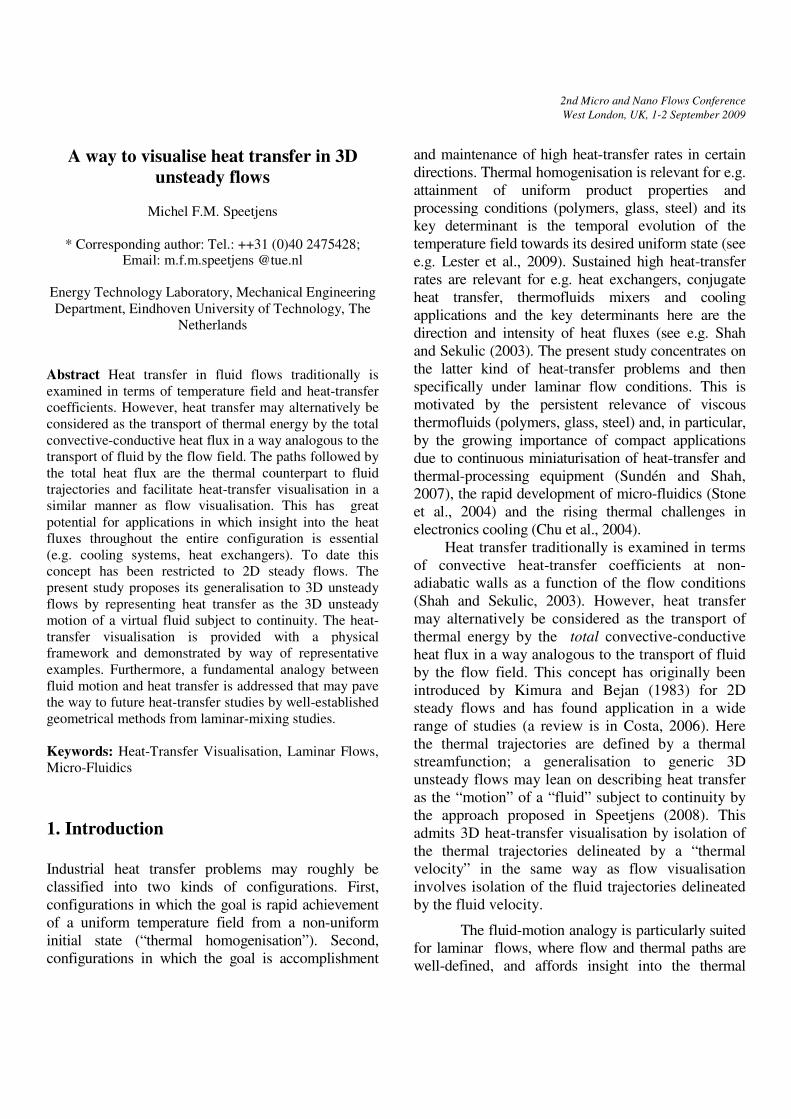
flow field. Figure 1a gives the resulting streamline

portrait, revealing the flow around the object and the

formation of a recirculation zone in its wake.



a) Streamline portrait

b) Temperature field

Fig. 1. 2D case study: (panel b: blue: T=0; red: T=1).

3.3 Heat-transfer visualisation: thermal streamlines

The present steady conditions reduce the energy

equation (1) to 0=⋅∇ Qv

, exposing the total heat flux

Qr

as solenoidal. Thus the energy equation takes the

same form as the steady-state continuity equation

underlying (2). This mathematical equivalence

naturally leads to the concept of a “thermal stream

function” TΨ , which is governed by

x

T Qy

=∂

Ψ∂, y

T Qx

−=∂

Ψ∂,, (3)

as the thermal analogy to the stream function Ψ .

The isopleths of TΨ delineate the sought-after

thermal transport routes and are the thermal

equivalent of the streamlines of the fluid flow (i.e.

“thermal streamlines”). The thermal streamline

portrait thus visualizes the heat transfer in essentially

the same way as the streamline portrait visualises the

fluid transport. This concept has originally been

introduced by Kimura and Bejan (1983) and has

found application in a wide range of studies (refer to

Costa, 2006 for a review).

The equivalence between (2) and (3) implies

a fundamental analogy between fluid and heat

transport. First, it advances the total heat flux Qr

as

the thermal counterpart to the mass flux Mv

. Second,

it implies that (the isopleths of) Ψ and TΨ are

subject to the same geometrical restrictions: the

(thermal) streamlines cannot suddenly emerge or

terminate; they must either be closed or connect with

a boundary. This has fundamental ramifications for

the transport properties in the sense that the

(thermal) streamlines are organised into coherent

structures that geometrically determine the fluid

motion and heat transfer. For the fluid motion this

manifests itself in the formation of a throughflow

region, consisting of “channels” that connect inlet

and outlet of the domain, and a recirculation zone

(Figure 1a). For the heat transfer a similar

organisation happens. This is demonstrated below.

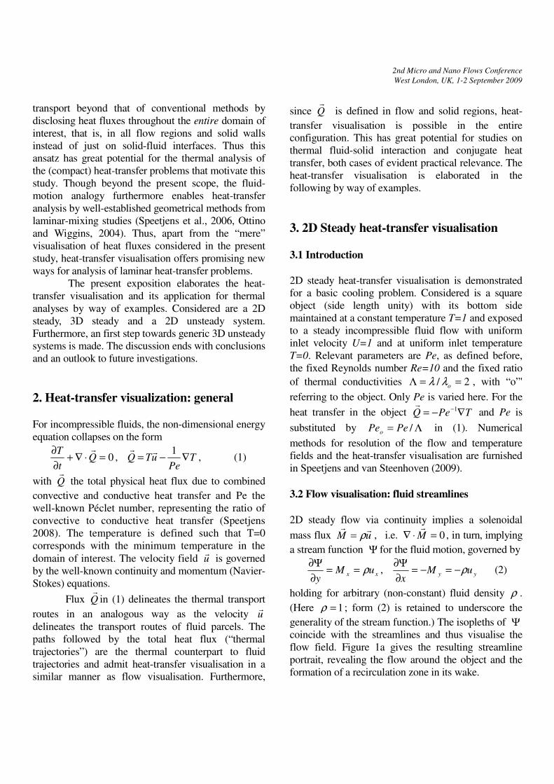
Fig. 2. 2D case study: thermal streamlines (Pe=50).

The temperature field is displayed in

Figure 1b and its distribution clearly reflects the

cooling of the object by the passing fluid. Figure 2

gives the corresponding thermal streamline portrait

TΨ . The thermal streamlines bound, similar to its

counterpart in the streamline portrait (Figure 1a),

adjacent channels. These channels transport thermal

energy in the same manner as stream tubes transport

fluid and are the thermal equivalent to stream tubes

(“heat conduits”). The fact that thermal streamlines

must either be closed or connect with a boundary

implies two kinds of heat conduits: (i) open heat

conduits connected with boundaries; (ii) closed heat

conduits. Both types are present in Figure 2 and their

role in the heat transfer is considered below.

The open heat conduits inside the object facilitate

the heat transfer from its hot bottom side through its

interior towards the fluid-solid interface. Here the

open heat conduits continue into the flow region and

collectively form a “plume” that emerges from the

perimeter of the object and rapidly aligns itself with

the flow in downstream direction. This plume



constitutes the “thermal path” by which heat is

removed from the object by the passing fluid. The

thermal path is bend around a family of concentric

closed heat conduits that collectively form a thermal

recirculation zone (“thermal island”). The thermal

island entraps and circulates thermal energy and,

consequently, forms a thermally-isolated region. The

blank region upstream of the thermal path has

negligible heat flux ( 0rr

≈Q ) and, consequently,

renders TΨ undefined (“thermally-inactive region”).

Thus heat-transfer visualisation exposes the several

relevant regions of the heat-transfer problem and puts

forth the thermal path as the only region actively

involved in the cooling process of the object.

3.4 Thermal path: the role of convection

Heat transfer in the flow region has two asymptotic

states: Pe=0 (purely-conductive heat transfer) and

∞→Pe (purely-convective heat transfer). The

actual state sits between both asymptotic states for

finite Pe and progresses from its conductive to its

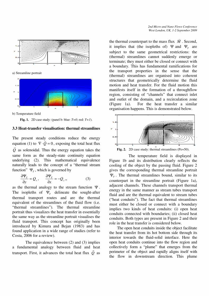
convective limit with rising Pe. This is demonstrated

in Figure 3. For the conductive state (panel a) the

thermal path occupies the entire flow region,

signifying heat release into the entire domain and has

two sections, separated by a separatrix emanating

from the top wall of the object (not shown), the left

and right of which transport heat to inlet and outlet,

respectively, of the flow region. The separatrix

propagates towards the lower-left corner of the

object (panel b) with rising Pe until one thermal path

connecting object with outlet forms (panel c).

Furthermore, the thermal island emerges in the wake

of the object and the thermal path becomes spatially

more confined (panel d).

4. 3D Steady heat-transfer visualisation

4.1 Introduction

Here the 3D extension to the above cooling problem

is considered. The configuration consists of a cubical

object (side length unity) with its bottom side

maintained at a constant temperature T=1 and expo-

sed to a steady incompressible fluid flow with uni-

form inlet velocity U=1 and at uniform inlet tem-

perature T=0. The system parameters are identical to

those of the 2D counterpart. Numerical methods for

resolution of the 3D flow and temperature fields and

the 3D heat-transfer visualisation are furnished in

Speetjens and van Steenhoven (2009).

a) Pe=0

b) Pe=1

c) Pe=10

d) Pe=200

Fig. 3. Progression of the thermal streamline portrait with

increasing Pe.



4.2 Flow visualisation: 3D streamlines

Essential difference with the 2D case is that in the

3D case streamfunctions no longer exists. Here the

fluid streamlines )(tx are governed by

,uM

dt

xd==

ρ 0=⋅∇ M

r, (4)

with uMrr

ρ= the solenoidal mass flux as introduced

before. Hence, the fluid streamlines coincide with

the field lines of both ur

and Mr

. Note that (4) is a

generalisation of the streamfunction relation (2).

Continuity imposes the same geometrical

restrictions upon the 3D streamlines )(tx as found

before for the 2D case: the streamlines cannot

suddenly emerge or terminate; they must either be

closed or connect with a boundary. This manifests

itself, essentially similar to the 2D steady case, in the

fact that continuity organises the streamlines into

coherent structures, albeit of a greater variety and

complexity due to the larger geometric freedom

afforded by 3D conditions. These structures

determine the topological make-up (“flow

topology”) of the web of fluid trajectories

(Speetjensd at al., 2006, Malyuga et al., 2002). This

flow topology is the generalisation of the 2D

streamline portrait.

4.3 Heat-transfer visualisation: 3D thermal

streamlines

The analogy between (thermal) stream functions

Ψ and TΨ and mass and heat flux M

r and Q

established before naturally leads to

,TT

uT

Q

dt

xd== 0=⋅∇ Q , (5)

as thermal counterpart to (4) (Speetjens and van

Steenhoven, 2009). The mathematical equivalence

between (4) and (5) implies that heat transfer in

essence is the “motion” of a “fluid” with “density” T

propagating along thermal trajectories Tx

delineated by a “thermal velocity” Tu subject to

continuity. This, in turn, implies a “thermal

topology” as thermal counterpart to the flow

topology that is organised into the same kinds of

coherent structures as the latter. The concept of a 3D

thermal topology is exemplified below by the 3D

thermal path originating from the 3D object.

4.4 Thermal path revisited

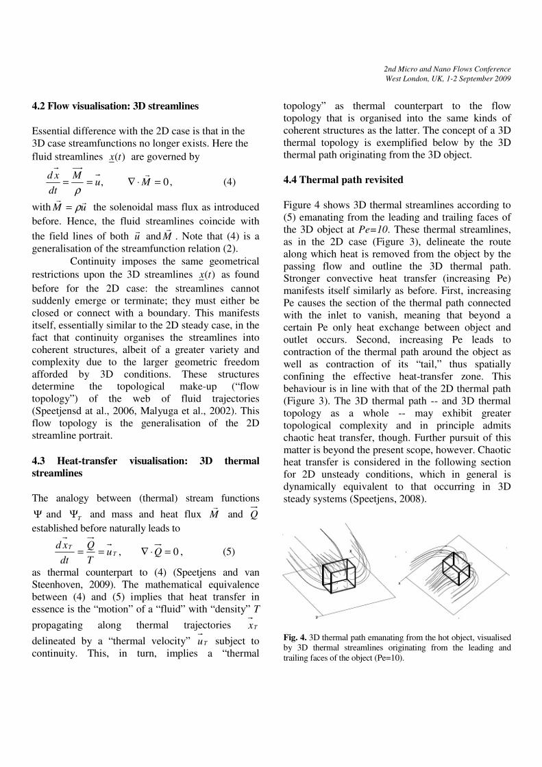
Figure 4 shows 3D thermal streamlines according to

(5) emanating from the leading and trailing faces of

the 3D object at Pe=10. These thermal streamlines,

as in the 2D case (Figure 3), delineate the route

along which heat is removed from the object by the

passing flow and outline the 3D thermal path.

Stronger convective heat transfer (increasing Pe)

manifests itself similarly as before. First, increasing

Pe causes the section of the thermal path connected

with the inlet to vanish, meaning that beyond a

certain Pe only heat exchange between object and

outlet occurs. Second, increasing Pe leads to

contraction of the thermal path around the object as

well as contraction of its “tail,” thus spatially

confining the effective heat-transfer zone. This

behaviour is in line with that of the 2D thermal path

(Figure 3). The 3D thermal path -- and 3D thermal

topology as a whole -- may exhibit greater

topological complexity and in principle admits

chaotic heat transfer, though. Further pursuit of this

matter is beyond the present scope, however. Chaotic

heat transfer is considered in the following section

for 2D unsteady conditions, which in general is

dynamically equivalent to that occurring in 3D

steady systems (Speetjens, 2008).

Fig. 4. 3D thermal path emanating from the hot object, visualised

by 3D thermal streamlines originating from the leading and

trailing faces of the object (Pe=10).



5. 2D Unsteady heat-transfer visualisation

5.1 Unsteady flow and heat-transfer visualisation

Relation (4) under unsteady conditions becomes

,uM

dt

xd==

ρ 0=⋅∇+

∂

∂M

t

rρ, (6)

and, via (1), naturally leads to

,TT

uT

Q

dt

xd== 0=⋅∇+

∂

∂Q

t

T, (7)

as its thermal equivalent, meaning the physical

analogy between fluid motion and heat transfer – and

flow and thermal topologies – established above is

upheld. The unsteady flow and thermal topologies,

governed by (6) and (7), respectively, are illustrated

hereafter for the heat transfer in a time-periodic flow

(period time 1=τ ) set up by a horizontally-

oscillating vortex pair inside a non-dimensional

periodic channel (width W=1; height H=1/2) with

hot bottom and cold top wall. The velocity field is

given by the analytical expressions

))(())(()1,(),( txutxutxutxu −+ +=+= , (8)

with )4/1),(()( /

0/ txxtx ∆−= −+−+ the positions of

the two adjacent vortices ( 4/10 =−x and 4/30 =+x )

and πε 2sin)( =∆ tx t the oscillation at amplitude

ε .The basic velocity reads yxxu x ππ 2cos2sin)( =

and yxxu y ππ 2sin2cos)( −= . System parameters are

the Péclet number Pe (here fixed at Pe=10) and the

amplitude ε . The employed numerical methods are

detailed in Speetjens and van Steenhoven (2009).

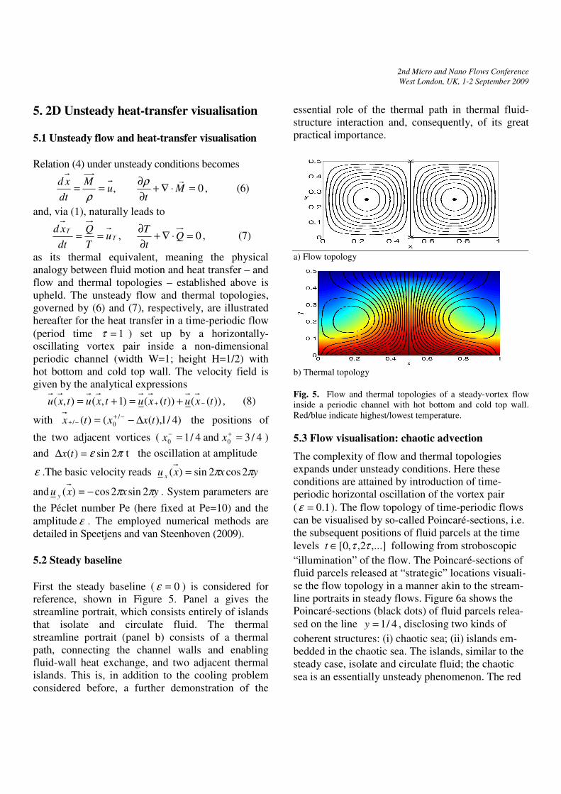
5.2 Steady baseline

First the steady baseline ( 0=ε ) is considered for

reference, shown in Figure 5. Panel a gives the

streamline portrait, which consists entirely of islands

that isolate and circulate fluid. The thermal

streamline portrait (panel b) consists of a thermal

path, connecting the channel walls and enabling

fluid-wall heat exchange, and two adjacent thermal

islands. This is, in addition to the cooling problem

considered before, a further demonstration of the

essential role of the thermal path in thermal fluid-

structure interaction and, consequently, of its great

practical importance.

a) Flow topology

b) Thermal topology

Fig. 5. Flow and thermal topologies of a steady-vortex flow

inside a periodic channel with hot bottom and cold top wall.

Red/blue indicate highest/lowest temperature.

5.3 Flow visualisation: chaotic advection

The complexity of flow and thermal topologies

expands under unsteady conditions. Here these

conditions are attained by introduction of time-

periodic horizontal oscillation of the vortex pair

( 1.0=ε ). The flow topology of time-periodic flows

can be visualised by so-called Poincaré-sections, i.e.

the subsequent positions of fluid parcels at the time

levels ,...]2,,0[ ττ∈t following from stroboscopic

“illumination” of the flow. The Poincaré-sections of

fluid parcels released at “strategic” locations visuali-

se the flow topology in a manner akin to the stream-

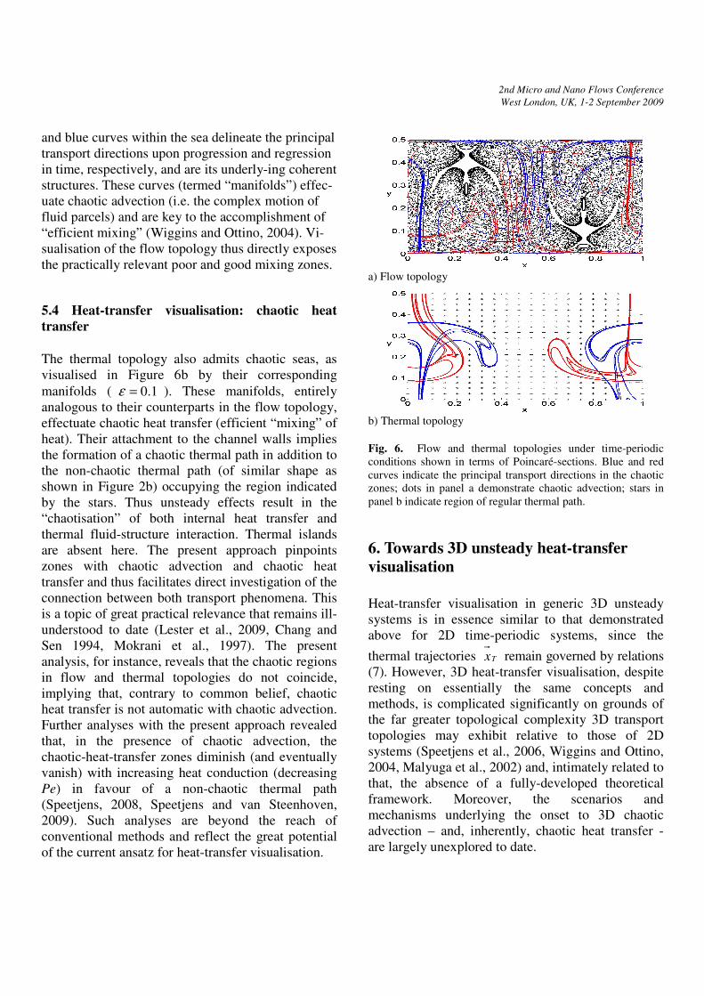
line portraits in steady flows. Figure 6a shows the

Poincaré-sections (black dots) of fluid parcels relea-

sed on the line 4/1=y , disclosing two kinds of

coherent structures: (i) chaotic sea; (ii) islands em-

bedded in the chaotic sea. The islands, similar to the

steady case, isolate and circulate fluid; the chaotic

sea is an essentially unsteady phenomenon. The red



and blue curves within the sea delineate the principal

transport directions upon progression and regression

in time, respectively, and are its underly-ing coherent

structures. These curves (termed “manifolds”) effec-

uate chaotic advection (i.e. the complex motion of

fluid parcels) and are key to the accomplishment of

“efficient mixing” (Wiggins and Ottino, 2004). Vi-

sualisation of the flow topology thus directly exposes

the practically relevant poor and good mixing zones.

5.4 Heat-transfer visualisation: chaotic heat

transfer

The thermal topology also admits chaotic seas, as

visualised in Figure 6b by their corresponding

manifolds ( 1.0=ε ). These manifolds, entirely

analogous to their counterparts in the flow topology,

effectuate chaotic heat transfer (efficient “mixing” of

heat). Their attachment to the channel walls implies

the formation of a chaotic thermal path in addition to

the non-chaotic thermal path (of similar shape as

shown in Figure 2b) occupying the region indicated

by the stars. Thus unsteady effects result in the

“chaotisation” of both internal heat transfer and

thermal fluid-structure interaction. Thermal islands

are absent here. The present approach pinpoints

zones with chaotic advection and chaotic heat

transfer and thus facilitates direct investigation of the

connection between both transport phenomena. This

is a topic of great practical relevance that remains ill-

understood to date (Lester et al., 2009, Chang and

Sen 1994, Mokrani et al., 1997). The present

analysis, for instance, reveals that the chaotic regions

in flow and thermal topologies do not coincide,

implying that, contrary to common belief, chaotic

heat transfer is not automatic with chaotic advection.

Further analyses with the present approach revealed

that, in the presence of chaotic advection, the

chaotic-heat-transfer zones diminish (and eventually

vanish) with increasing heat conduction (decreasing

Pe) in favour of a non-chaotic thermal path

(Speetjens, 2008, Speetjens and van Steenhoven,

2009). Such analyses are beyond the reach of

conventional methods and reflect the great potential

of the current ansatz for heat-transfer visualisation.

a) Flow topology

b) Thermal topology

Fig. 6. Flow and thermal topologies under time-periodic

conditions shown in terms of Poincaré-sections. Blue and red

curves indicate the principal transport directions in the chaotic

zones; dots in panel a demonstrate chaotic advection; stars in

panel b indicate region of regular thermal path.

6. Towards 3D unsteady heat-transfer

visualisation

Heat-transfer visualisation in generic 3D unsteady

systems is in essence similar to that demonstrated

above for 2D time-periodic systems, since the

thermal trajectories Tx remain governed by relations

(7). However, 3D heat-transfer visualisation, despite

resting on essentially the same concepts and

methods, is complicated significantly on grounds of

the far greater topological complexity 3D transport

topologies may exhibit relative to those of 2D

systems (Speetjens et al., 2006, Wiggins and Ottino,

2004, Malyuga et al., 2002) and, intimately related to

that, the absence of a fully-developed theoretical

framework. Moreover, the scenarios and

mechanisms underlying the onset to 3D chaotic

advection – and, inherently, chaotic heat transfer -

are largely unexplored to date.



7. Conclusions

The study proposes an approach by which to visualise

heat transfer in 3D unsteady laminar flows. This

approach hinges on considering heat transfer as the

transport of thermal energy by the total convective-

conductive heat flux in a way analogous to fluid

transport by the flow field. The paths followed by the

total heat flux are the thermal counterpart to fluid

trajectories and facilitate heat-transfer visualisation in

a similar manner as flow visualisation. This has great

potential for applications in which insight into the heat

fluxes throughout the entire configuration is essential.

To date this concept has been restricted to 2D steady

flows. The present study proposes its generalisation to

3D unsteady flows by representing heat transfer as the

3D unsteady “motion” of a “fluid” subject to

continuity. This affords insight into the thermal

transport beyond that of conventional methods.

2D steady heat-transfer visualization centres

on a “thermal stream function” that, analogous to the

fluid stream function delineating the fluid

streamlines, delineates the thermal transport routes

(“thermal streamlines”). The thermal streamline

portraits are, by virtue of continuity, organised into

two kinds of coherent structures: thermal islands and

thermal paths. Thermal islands consist of closed

thermal streamlines and entrap and circulate heat.

Thermal paths consist of open thermal streamlines

attached to non-adiabatic walls and facilitate net heat

exchange between these walls and the flow. Thermal

paths thus are key to many practical heat-transfer

problems.

The thermal topology in 3D steady systems is

organised into similar coherent structures as in 2D

systems, the most important of which again is the

thermal path emanating from non-adiabatic walls.

However, 3D systems may exhibit greater topological

complexity and in principle admit chaotic advection

and chaotic heat transfer. 2D unsteady systems are

dynamically similar to 3D steady systems and also

admit chaotic transport. The connection between

chaotic advection and chaotic heat transfer is highly

non-trivial, though. Thermal topologies in 3D

unsteady systems, though admitting visualisation by

essentially the same methods as their 2D counterparts,

may exhibit an even greater topological complexity.

Hence, their properties remain largely unexplored to

date and are the subject of ongoing investigations.

The analogy between heat transfer and fluid

motion facilitates analysis of heat-transfer problems

by well-established geometrical methods from

laminar mixing. This offers promising new ways for

analysis of laminar heat-transfer problems. Studies to

address these issues are in progress.

References

Lester, D. R., Rudman, M., Metcalfe, G., 2009. Low Reynolds

number scalar transport enhancement in viscous and non-

Newtonian fluids. Int. J. Heat Mass Transfer, 655.

Shah, R.K., Sekulic, D.P., 2003. Fundamentals of Heat

Exchanger Design. Wiley, Chichester.

Sundén, B., Shah, R.K., 2007. Advances in Compact Heat

Exchangers, Edwards. Philadelphia.

Stone, H. A., Stroock, A. D., Ajdari, A., 2004. Engineering

flows in small devices: microfluidics toward a lab-on-a-

chip. Ann. Rev. Fluid Mech. 36, 381.

Ottino, J. M. ,Wiggins, S., 2004. Introduction: mixing in micro-

fluidics. Phil. Trans. R. Soc. Lond. A 362, 923.

Chu, R. C., Simons, R. E., Ellsworth, M. J., Schmidt, R. R.,

Cozzolino, V., 2004. Review of cooling technologies for

computer products. IEEE Trans. Device Mat. Reliab. 4, 568.

Kimura, S. , Bejan, A., 1983. The heatline visualization of

convective heat transfer. ASME J. Heat Transfer 105, 916.

Costa, V.A.F., 2006. Bejan's heatlines and masslines for con-

vection visualization and analysis. ASME Appl. Mech.

Rev. 59, 126.

Speetjens, M.F.M. , 2008. Topology of advective-diffusive scalar

transport in laminar flows. Phys. Rev. E 77, 026309.

Speetjens, M., Metcalfe, G., Rudman, M., 2006. Topological

mixing study of non-Newtonian duct flows. Phys. Fluids 18,

103103.

Wiggins, S., Ottino, J.M., 2004. Foundations of chaotic mixing.

Phil. Trans. R. Soc. Lond. A 362, 937.

Malyuga, V. S., Meleshko, V. V., Speetjens, M. F. M., Clercx,

H. J. H., van Heijst, G. J. F., 2002. Mixing in the Stokes

flow in a cylindrical container. Proc. R. Soc. Lond. A 458,

1867.

Speetjens, M.F.M., van Steenhoven, A.A., 2009. A way to

visualise laminar heat-transfer in 3D unsteady flows.

Submitted to Int. J. Heat Mass Transfer.

Chang, H.-C., Sen, M., 1994. Application of chaotic advection to

heat transfer. Chaos, Solitons & Fractals 4, 955.

Mokrani, A., Casterlain, C., Peerhossaini, H., 1997. The effects of

chaotic advection on heat transfer. Int. J. Heat Mass Transfer

40, 3089.

Documents

A way to visualise heat transfer in 3D and maintenance of ...bura.brunel.ac.uk/bitstream/2438/6868/1/MNF2009.pdf · A way to visualise heat transfer in 3D ... the heat transfer from