A Zonal Method for Modeling Powered-Lift Aircraft Flow · PDF fileNASA Contractor Report 177521 . A Zonal Method for Modeling Powered-Lift Aircraft Flow Fields \ D. W. Roberts Arntec

$Page 1: A Zonal Method for Modeling Powered-Lift Aircraft Flow · PDF fileNASA Contractor Report 177521 . A Zonal Method for Modeling Powered-Lift Aircraft Flow Fields \ D. W. Roberts Arntec$
NASA Contractor Report 177521

. A Zonal Method for Modeling Powered-Lift Aircraft Flow Fields

\

D. W. Roberts

Arntec Engineering, Inc. 11 820 Northup Way, Suite 200 Bellevue, WA 98005

Prepared for Arnes Research Center

March 1989 CONTRACT NAS2-12801

National Aeronautics and Space Administration

Ames Research Center Moffett Field, California 940%

https://ntrs.nasa.gov/search.jsp?R=19890014916 2018-05-26T01:13:56+00:00Z

Contents List of Figures iv

1 Summary

1 Introduction 2

2 Discussion 4 Descriptions of the Flow Code . . . . . . . . . . . . . . . . . . . . . . 4 2.1.1 3DNS . . . . . . . . . . . . . . . . . . . . . . . . . . . . . . . 4 2.1.2 PMARC.. . . . . . . . . . . . . . . . . . . . . . . . . . . . . 6

2.2 Boundary Condition Specification . . . . . . . . . . . . . . . . . . . . 7 2.3 Interzone Boundary Positions . . . . . . . . . . . . . . . . . . . . . . 8 2.4 Modifications to PMARC . . . . . . . . . . . . . . . . . . . . . . . . 9 2.5 Modifications to 3DNS . . . . . . . . . . . . . . . . . . . . . . . . . . 10 2.6 Automated Coupling Procedure . . . . . . . . . . . . . . . . . . . . . 14

2.1

3 Test Cases 16 16 16 19 20

3.1 Coupled PMARC/3DNS Cases . . . . . . . . . . . . . . . . . . . . . 3.1.1 Axisymmetric Jet . . . . . . . . . . . . . .. . . . . . . . . . . . 3.1.2 Jet Impingement . . . . . . . . . . . . . . . . . . . . . . . . . 3DNS to 3DNS Coupling. . . . . . . . . . . . . . . . . . . . . . . . . 3.2

4 Conclusions 22

5 Recommendations 23

PRECEDING PAGE BLANK NOT FILMED

iii

I List of Figures

1 2 3 4 5 6 7 8 9 10 11 12 13 14 15 16 17 18 19 20 21 22

23

24

25

26

27

28

29

30

Half cell overlap when interzone boundaries coincide . . . . . . . . .

Control loop for coupling PMARC and 3DNS . . . . . . . . . . . . . Schematic of zonal boundaries for axisymmetric jet . . . . . . . . . . Computational grid for 3DNS zone . Case 1 . . . . . . . . . . . . . . Computational grid for SDNS zone . Case 2 . . . . . . . . . . . . . . Computational grid for SDNS zone . Case 3 . . . . . . . . . . . . . . Computational grid for SDNS zone . Case 4 . . . . . . . . . . . . . . Computational grid for 3DNS zone . Case 5 . . . . . . . . . . . . . . Velocity vectors for SDNS zone . Case 1 . . . . . . . . . . . . . . . . Velocity vectors for SDNS zone . Case 2 . . . . . . . . . . . . . . . . Velocity vectors for 3DNS zone . Case 3 . . . . . . . . . . . . . . . . Velocity vectors for SDNS zone . Case 4 . . . . . . . . . . . . . . . . Velocity vectors for 3DNS zone . Case 5 . . . . . . . . . . . . . . . . Streamwise velocity contours for axisymmetric jet . . . . . . . . . . . Streamwise velocity profile for axisymmetric jet . . . . . . . . . . . . Convergence of the 3DNS zonal solutions . Case 1 . . . . . . . . . . Convergence of the 3DNS zonal solutions . Case 2 . . . . . . . . . . Convergence of the SDNS zonal solutions . Case 3 . . . . . . . . . . Convergence of the SDNS zonal solutions . Case 4 . . . . . . . . . . Convergence of the 3DNS zonal solutions . Case 5 . . . . . . . . . .

Case 1, 100 SDNS time steps/global iteration . . . . . . . . . . . . .


Case 1, 300 3DNS time steps/global iteration . . . . . . . . . . . . .







27 27 28 29 30 30 31 31 32 32 33 33 34 34 35 35 36 36 37 37 38

38

39

39

40

40

41

41

42

42

PMARC boundary formed from two grid surfaces in the 3DNS zone .

Normal velocity component distribution along PMARC boundary .









I I iv

31

32

33

34

35

36

37

38

39

40

41

42

43

44

45

46

47

48

49

50

Normal velocity component distribution along PMARC boundary -
















Normal velocity convergence versus coupling( global) iteration - Case 1. . . . . . . . . . . . . . . . . . . . . . . . . . . . . . . . . . . . . . Normal velocity convergence versus coupling( global) iteration - Case

Case 2, 500 SDNS time steps/global iteration.

Case 3, 100 3DNS time steps/global iteration.















. . . . . . . . . . . .

. . . . . . . . . . . .

. . . . . . . . . . . .

. . . . . . . . . . . .

. . . . . . . . . . . .

. . . . . . . . . . . .

. . . . . . . . . . . .

. . . . . . . . . . . .

. . . . . . . . . . . .

. . . . . . . . . . . .

. . . . . . . . . . . .

. . . . . . . . . . . .

. . . . . . . . . . . .

. . . . . . . . . . . .

. . . . . . . . . . . .

. . . . . . . . . . . .

2. . . . . . . . . . . . . . . . . . . . . . . . . . . . . . . . . . . . . . Normal velocity convergence versus coupling(g1oba.l) iteration - Case 3. . . . . . . . . . . . . . . . . . . . . . . . . . . . . . . . . . . . . . Normal velocity convergence versus coupling( global) iteration - Case 4. . . . . . . . . . . . . . . . . . . . . . . . . . . . . . . . . . . . . .

43

43

44

44

45

45

46

46

47

47

48

48

49

49

50

50

5 1

51

52

52

V

51

52

53

54

55

56

57 58 59 60 61 62 63 64 65 66 67

Normal velocity convergence versus coupling(gl0bal) iteration . Case 5 . . . . . . . . . . . . . . . . . . . . . . . . . . . . . . . . . . . . . . Normal velocity convergence versus 3DNS time steps/global iteration .Case1 . . . . . . . . . . . . . . . . . . . . . . . . . . . . . . . . . . Normal velocity convergence versus 3DNS time steps/global iteration .Case2 . . . . . . . . . . . . . . . . . . . . . . . . . . . . . . . . . . Normal velocity convergence versus 3DNS time steps/global iteration .Case3 . . . . . . . . . . . . . . . . . . . . . . . . . . . . . . . . . . Normal velocity convergence versus 3DNS time steps/global iteration .Case4 . . . . . . . . . . . . . . . . . . . . . . . . . . . . . . . . . . Normal velocity convergence versus 3DNS time steps/global iteration .Case5 . . . . . . . . . . . . . . . . . . . . . . . . . . . . . . . . . . Schematic of jet impingement configuration for coupled analysis . . . Entrainment induced streamlines in the PMARC zone . . . . . . . . Suckdown pressure decrement on vehicle base due to entrainment . . 2-D convergent-divergent thrust-reversing nozzle . . . . . . . . . . . Computational zonal grid for thrust-reversing nozzle . . . . . . . . . Calculated pressure contours . . . . . . . . . . . . . . . . . . . . . . Close-up of pressure contours at zonal boundary . . . . . . . . . . . . Calculated velocity vectors . . . . . . . . . . . . . . . . . . . . . . . . Close-up of velocity vectors at zonal boundary . . . . . . . . . . . . . Streamlines in the thrust-reverser flow field near the zonal boundary . Comparison of pressure distributions on thrust-reverser blocker . . .

53

53

54

54

55

55 56 57 57 58 58 59 59 60 60 61 61

vi

SUMMARY

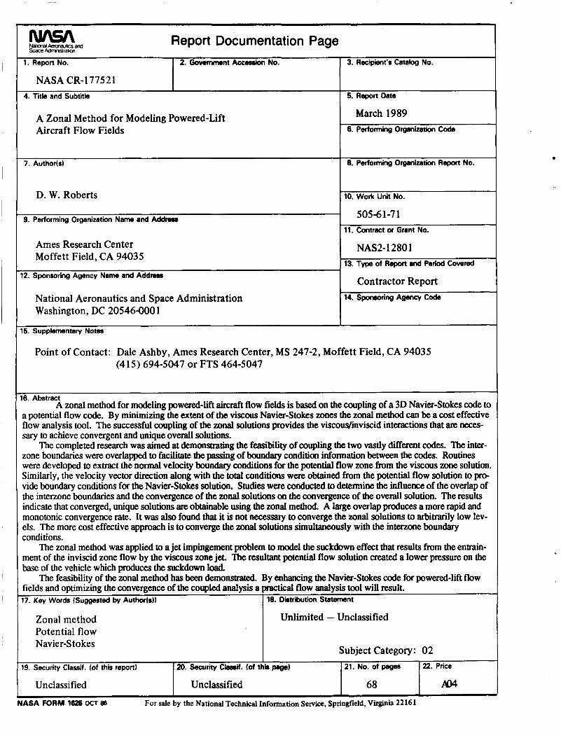
A zonal method for modeling powered-lift aircraft flow fields is based on the coupling of a 3D Navier-Stokes code to a potential flow code. By minimizing the extent of the viscous Navier-Stokes zones the zonal method can be a cost effective flow analysis tool. The successful coupling of the zonal solutions provides the viscous/inviscid interactions that are necessary to achieve convergent and unique overall solutions.

The completed research was aimed at demonstrating the feasibility of coupling the two vastly different codes. The interzone boundaries were overlapped to facil- itate the passing of boundary condition information between the codes. Routines were developed to extract the normal velocity boundary conditions for the potential flow zone from the viscous zone solution. Similarly, the velocity vector direction along with the total conditions were obtained from the potential flow solution to provide boundary conditions for the Navier-Stokes solution. Studies were conducted to determine the influence of the overlap of the interzone boundaries and the convergence of the zonal solutions on the convergence of the overall solution. The results indicate that converged, unique solutions are obtainable using the zonal method. A large overlap produces a more rapid and monotonic convergence rate. It was also found that it is not necessary to converge the zonal solutions to arbitrarily low levels. The more cost effective approach is to converge the zonal solutions simultaneously with the interzone boundary conditions.

The zonal method was applied to a jet impingement problem to model the suckdown effect that results from the entrainment of the inviscid zone flow by the viscous zone jet. The resultant potential flow solution created a lower pressure on the base of the vehicle which produces the suckdown load.

The feasibility of the zonal method has been demonstrated. By enhancing the Navier-Stokes code for powered-lift flow fields and optimizing the convergence of the coupled analysis a practical flow analysis tool will result.

1

1 Introduction

Powered-lift aircraft are designed to use exhaust jets to directly increase lift. Con- cepts [l-71 include vertical jets, vectored nozzles, jet flaps, upper surface blowing (USB) and ejectors to name a few. The flow fields generated by these jets are three-dimensional and dominated by viscous effects. When the jets interact with the ground plane, which is common during take-d, hover, and landing modes, the flow fields become even more complex. Wall jets, ground vortices, fountain flow and other phenomena [8,9] can have a significant influence on the performance and stability of powered-lift aircraft. Currently, most of these flow fields are examined by wind tunnel tests, which tend to be time-consuming and expensive. The need exists for a cost effective flow analysis tool to numerically model powered-lift flow fields.

To model all of the complex flow phenomena, the Navier-Stokes equations with appropriate modeling of the Reynolds stress terms for turbulent flows must be solved. Though the technology may exist for solving the Navier-Stokes equations for a complete aircraft flow domain, the substantial requirements for computer resources to achieve an accurate simulation would be prohibitive for practical usage. Subsets of the Navier-Stokes equations, such as the potential flow equation, the parabolized Navier-Stokes equations, the boundary layer equations, and the Euler equations, are often appropriate for large regions of the flow domain while costing much less in terms of computer time and storage. The physics supplied by the full set of Navier-Stokes equations usually are only required in a small portion of the flow domain. In view of this, a zonal method is the preferred approach for developing a cost effective numerical flow analysis procedure.

I

I

~

With the zonal method the flow domain is divided into a network of zones. In each zone the simplest physically appropriate flow analysis code is used to model the flow. The positioning of the zonal boundaries is based on the complexity of the local flow phenomena and on the geometry of the configuration under consideration. The zone boundaries are chosen to minimize the portion of the domain in which the more expensive Navier-Stokes equation solver is used and, conversely, to maximize the use of the simpler (yet appropriate) numerical flow analyses. The zonal solutions are iteratively coupled at their boundaries to yield a converged, physically accurate solution for the complete flow field. The zone boundaries are also chosen to ease the generation of the computational mesh. For example, the mesh for a domain with many distinct geometric shapes, such as the internal ducting found in powered-lift vehicles, can be generated more easily by a network of distinct meshes than by one large complex mesh.

2

The fundamental benefit of the zonal method is the efficient use of computer resources (including CPU time) by implementing the simplest numerical analysis in each zone while achieving a valid solution for the full domain. A substantial computer and manpower savings also results from the simplified mesh generation approach. Furthermore, existing flow analysis codes can be used as modules in the zonal method, eliminating the need to develop new codes for new geometries.

The key feature of a zonal method is the coupling of the zonal solutions across the interzonal boundaries. This is not a difficult task when one flow code is used for the solution in all zones. When different codes are coupled, it is important that appropriate boundary condition data be passed between the codes and that the interzone boundaries are positioned correctly. Several zonal methods [ 10-171 have been developed to model viscous/inviscid flow interactions, but these have mainly been limited to 2D calculations or to the use of boundary layer or parabolized Navier-Stokes codes in the viscous zones. The scope of the present investigation was aimed at developing a procedure for coupling two vastly different codes which would form the foundation for a zonal method for powered-lift aircraft flow fields. A three-dimensional full Navier-Stokes code is used to model the viscous zones. The surrounding inviscid flow zone is modeled with a potential flow code based on panel methodology, which is sufficient for low-speed flight. These codes are both elliptic which means that any perturbation of a boundary condition will be felt throughout the zonal solution. The panel method views the viscous zones as extensions of the configuration. They influence the inviscid zone through blockage, which is an inviscid effect, and through entrainment, which is the result of viscosity. Similarly, the viscous zones are influenced by the dynamics of the inviscid zone flow field. The coupling procedure that was developed provides the correct interaction between zonal solutions and leads to convergent and consistent overall solutions. The following sections provide descriptions of the codes, the coupling boundary conditions, the coupling procedure, and results of test cases using the coupled analysis.

3

2 Discussion

2.1 Descriptions of the Flow Code

The zonal method couples the flow solutions in viscous and inviscid zones. In each zone the appropriate flow analysis code is activated to model the physics associated with that zone. A 3D Navier-Stokes code, SDNS, was chosen for the viscous zones since the full Navier-Stokes equations can model the wide range of flow phenomena associated with powered-lift aircraft. The 3DNS code was developed by Amtec Engineering and can be easily modified due to its modular structure. The PMARC code, a potential flow analysis based on panel methodology, was selected for modeling the inviscid zone. The potential flow equation is appropriate for low speed aerodynamics. PMARC is a panel code supported by NASA-ARC. Since the PMARC source code is available, modifications and extensions can be made to allow coupling. The following sections provide a brief overview of each code.

2.1.1 3DNS

The Amtec SDNS code uses a mesh built up from multiple i , j , k ordered grids (zones) patched together. The patched grid gives a better discretization of a complex flow domain than can be achieved with a single z,j, IC ordered grid.

I

I

The SDNS code solves the mass-averaged form of the Reynolds-averaged Navier- Stokes equations. These equations are given below in integral form [18].

I

where

and

I

4

N = (0)

E = p e+-u,u = p H - p [ f . j I

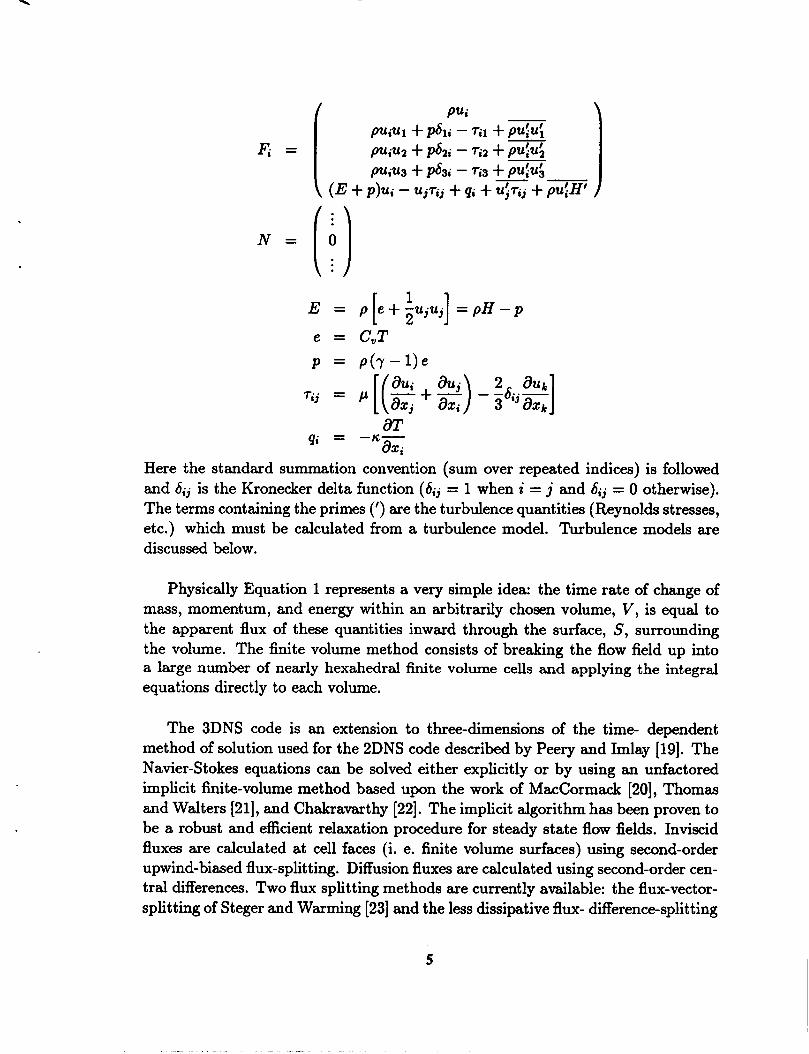
Here the standard summation convention (sum over repeated indices) is followed and Sij is the Kronecker delta function ( S i j = 1 when i = j and Sij = 0 otherwise). The terms containing the primes (') are the turbulence quantities (Reynolds stresses, etc.) which must be calculated from a turbulence model. Turbulence models are discussed below.

Physically Equation 1 represents a very simple idea: the time rate of change of mass, momentum, and energy within an arbitrarily chosen volume, V, is equal to the apparent flux of these quantities inward through the surface, S, surrounding the volume. The finite volume method consists of breaking the flow field up into a large number of nearly hexahedral finite volume cells and applying the integral equations directly to each volume.

The 3DNS code is an extension to three-dimensions of the time- dependent method of solution used for the 2DNS code described by Peery and Imlay [19]. The Navier-Stokes equations can be solved either explicitly or by using an unfactored implicit finite-volume method based upon the work of MacCormack [20], Thomas and Walters [21], and Chakravarthy [22]. The implicit algorithm has been proven to be a robust and efficient relaxation procedure for steady state flow fields. Inviscid fluxes are calculated at cell faces (i. e. finite volume surfaces) using second-order upwind-biased flux-split ting. Diffusion fluxes are calculated using second-order cen- tral differences. Two flux splitting methods are currently available: the flux-vector- splitting of Steger and Warming [23] and the less dissipative flux- difference-splitting

5

of Roe [24]. Linearizing the resulting difference equations forms a system of algebraic equations having a block banded coefficient matrix. Due to the near diagonal dominance of this matrix resulting from the flux splitting, this system of equations may be solved using a line- Gauss-Seidel iteration procedure. Only two to four iterations of the line-Gauss-Seidel are necessary to maintain numerical stability before updating the flow field variables and taking another time step. The resulting time marching scheme is very efficient and usually results in converged solutions in approximately 100 time steps. Mixing-length turbulence models [25] are currently used for calculating turbulent eddy viscosities in boundary layers and mixing layers.

The 3DNS code is structured so that it is efficient, easy to modify, and easy to maintain. The subroutines are organized using a layered approach which mod- ularizes the code according to function. This makes the code comparatively easy to debug and, therefore, reduces the time required to make a modification. As a result, efficient use will be made of the time and money supplied for the proposed R&D effort. The field variable data for all zones are stored in a HEAP (a one- dimensional array) in the upper level routines and are passed using pointers to the lower level routines where they are converted to multiple-dimension arrays. This results in no memory being wasted, even though the i , j , k dimensions of the different zones are unrelated. Utilities are provided for swapping zones to secondary memory and rearranging zonal data on the heap. In this manner, large problems can be accommodated by having only a small number of zones in main memory at a time.

2.1.2 PMARC

The PMARC solution is based upon the assumption that a velocity potential field exists which satisfies Laplace’s equation in the flow field of interest.

V2@ = 0

where @ is the velocity potential. By applying Green’s Theorem an integral equation for @ at any point in the flow field can be formed. The integrated quantities are the contributions from the distributed doublets and sources on the surface of the configuration being modeled. The doublets represent the local jump in potential and the sources represent the local jump in the normal component of velocity. On solid surfaces the source term forces a zero resultant normal velocity component

6

on the surface. To represent entrainment the source term forces a nonzero normal velocity equal to the entrained flow.

The surface is represented by a set of quadrilateral panels which discretize the distributions of doublets and sources. Each panel has a control point at which the potential flow solution is satisfied. The doublet and source distributions are assumed to be constant on each panel. The surface integrals for the velocity potential are transformed into a set of simultaneous linear algebraic equations for the doublet strength on each panel. This leads to a very large dense matrix problem. PMARC uses an iterative solver to obtain a solution. With the doublet strengths known the surface velocity field is determined. Off-body velocity surveys can be performed after the solution is known. This feature is crucial to the procedure for coupling PMARC with 3DNS.

2.2 Boundary Condition Specification

The key ingredient in the development of a successful coupling procedure is the transfer of useful information between zones in order to achieve a converged overall solution. When dealing with two distinctly different flow codes, such as PMARC and 3DNS, what is useful to one code is not appropriate for the other. PMARC models the flow field in its zone with the linearized potential flow equation, which is derived from the incompressible continuity equation. This mathematical model limits the physics that may be accurately simulated to irrotational flow. Since the flow is isentropic, the total pressure and temperature will be constant throughout the PMARC domain. This precludes using the total conditions for transferring information to a PMARC zone. Since continuity is satisfied by PMARC, a mass flux boundary condition provides the necessary, physically appropriate information that quantifies the influence of the viscous 3DNS zone on the PMARC solution. In PMARC this type of boundary condition is enforced by specifying the normal velocity components for the panels that form the boundary to the 3DNS zone. These normal velocities must be extracted from the 3DNS solution.

The 3DNS code models the flow field in the viscous zone with the complete compressible Navier-Stokes equations. Assuming an appropriate turbulence model to close the set of equations for turbulent flows, this flow analysis provides physically accurate simulations for virtually all flow fields of interest for powered-lift aircraft. Since the 3DNS code solves more equations than PMARC, it requires more information to completely specify the boundary conditions. The total pressure and temperature are automatically available from PMARC as discussed above.

7

PMARC can also provide the velocity vectors along the boundary, which are provided to the 3DNS code as the direction cosines that define the angle of the velocity vector. Specifying the velocity magnitude would lead to an over-specification of the boundary conditions. It is important to allow pressure waves to pass through the boundary. This would not be possible if the velocity magnitude was fixed. Hence, the most useful information to be provided by PMARC along the 3DNS boundary is the total pressure, total temperature, and the direction cosines of the velocity vector. Compatibility relations or extrapolation from within the 3DNS are used to obtain any other field variables that are required at the zone boundaries 88 discussed in section 2.5.

2.3 Interzone Boundary Positions

The positions of the interzone boundaries can have a significant influence on the success of the coupled analysis. To be physically accurate the interzone boundaries must be placed in a region of the flow domain where both codes can model all of the local physics. Since the potential flow equation is a subset of the Navier -Stokes equations, the PMARC interzonal boundary determines where the coupling should take place. Clearly, the PMARC boundary cannot be positioned in a shear layer. It should be in a region where viscous effects are negligible, but close enough to the shear layers to minimize the extent of the 3DNS zone for computational efficiency. The basic requirement is to size the SDNS zone such that it will include all of the dominant viscous interactions in the region of interest.

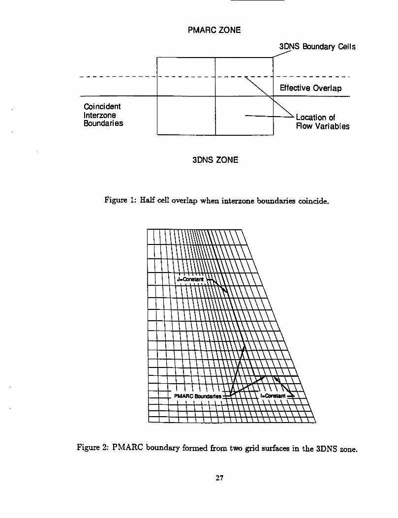
The effect of the amount of overlapping of the PMARC and SDNS interzone boundaries was examined as part of the current investigation. Coincident boundaries can lead to converged coupled solutions. In effect, this creates a half cell overlap since the flow variables in the SDNS zone are located at the computational cell centers, Figure 1. This may adversely effect convergence since the computed flow next to a zone boundary is strongly influenced by the boundary conditions. A poor initial guess for the boundary conditions is more likely to cause a strong perturbation in the zonal flow solutions when the interzonal boundaries are coincident. However, when the interzone boundaries overlap a significant distance into the adjacent zone, the boundary conditions provided by one zone to the other should transmit a better representation of the flow field in each zone. An evaluation of the influence of coincident interzonal boundaries on the coupled solution was not possible during the current investigation. The original PMARC routine for extract- ing flow field data at off-body points did not perform reliably when the specified points were in close proximity to the panels defining the boundary of the PMARC

8

zone. The routine worked satisfactorily when the points were a sufficient distance from the panels. Therefore, an interzonal boundary overlap of several cells could be investigated.

The approach taken was to specify the position of the PMARC interzone boundary. The PMARC boundary was defined to coincide with the surface formed by the grid points in the 3DNS zone having a constant index; i.e. the index J = constant. These mesh points formed the rows and columns of panels on the boundary. The distance between the PMARC boundary and the jet shear layer could be controlled to some degree. The overlap distance and the number of mesh cells between the interzone boundaries could be adjusted to control the position of the 3DNS boundary.

2.4 Modifications to PMARC

In order to implement the coupling procedure in which the boundary condition data is passed between the PMARC and SDNS codes, it was necessary to modify the PMARC code. Since the original PMARC code was an early version which was not well documented, this was a difficult task. Most of the large common blocks in PMARC were used as scratch space for temporary storage of variables in the various subroutines. As such the array memory space was different in several of the subroutines in which the common blocks were used. This inconsistency presented a problem since our inhouse computer does not allow variable length common blocks. It was important to be able to use our computer for interactive debugging. Therefore, it was necessary to pad the common blocks with dummy arrays.

Modifications were also made to the input/output routines. Open statements were added for the 1/0 files, which allows descriptive names to be given to the files. The input data was divided into five files based on the function of the data. Unit 28 was created to contain the program control parameters which are in the NAMELIST format. Unit 5 contained the geometry specification data for the configuration. Unit 99 contained the geometry description for the PMARC interzone boundary plus any other related panel patches. Unit 56 contained the specified normal velocity components for the panels that form the PMARC interzone boundary. Unit 32 contained the mesh points that formed the 3DNS interzone boundary. One additional output file, unit 31, was created to transmit to the SDNS code the velocity vector angle data for the off-body points input from unit 32.

9

The coupling of the PMARC and 3DNS codes requires the automated transfer of large amounts of boundary condition data. It is not reasonable to transmit this data using NAMELIST or by hand when several iterations of the coupling procedure are required. For this reason, subroutine GEOMIN was modified to input the jet boundary definition from unit 99. Subroutine SURPAN was modified to read the normal velocity for each panel from unit 56 when a flag is set to indicate that the file is available. Similarly, subroutine VSCAN was modified to read the off-body velocity scan points from unit 32. Write statements were added to output the velocity vector direction cosines to unit 31 in the format required by the 3DNS code.

Subroutine VEL is used to calculate the velocity components at each of the off-body scan points. Initially, this routine produced inconsistent and erroneous values. By systematically debugging the subroutine it was discovered that several of the arrays were not initialized with the necessary data before being used. The standard practice in PMARC is to store arrays locally in scratch common blocks, but keep them permanently in files as a means to create a type of a ‘virtual’ memory. For Cray-class computers this practice is inefficient and not necessary for most arrays except the influence coefficients which can require substantial storage. After determining which file contained the required data, the local arrays in VEL were filled and the results became acceptable. An exception occurred for off-body points that were very close to panels. The near field capability did not work reliably and, therefore, was avoided.

2.5 Modifications to 3DNS

The modifications to the 3DNS code included routines to define the interzone boundaries, to generate the panel system and normal velocities for individual panels on the PMARC boundary, and to specify the 3DNS boundary points to be used in scanning the PMARC solution to obtain the boundary conditions for 3DNS.

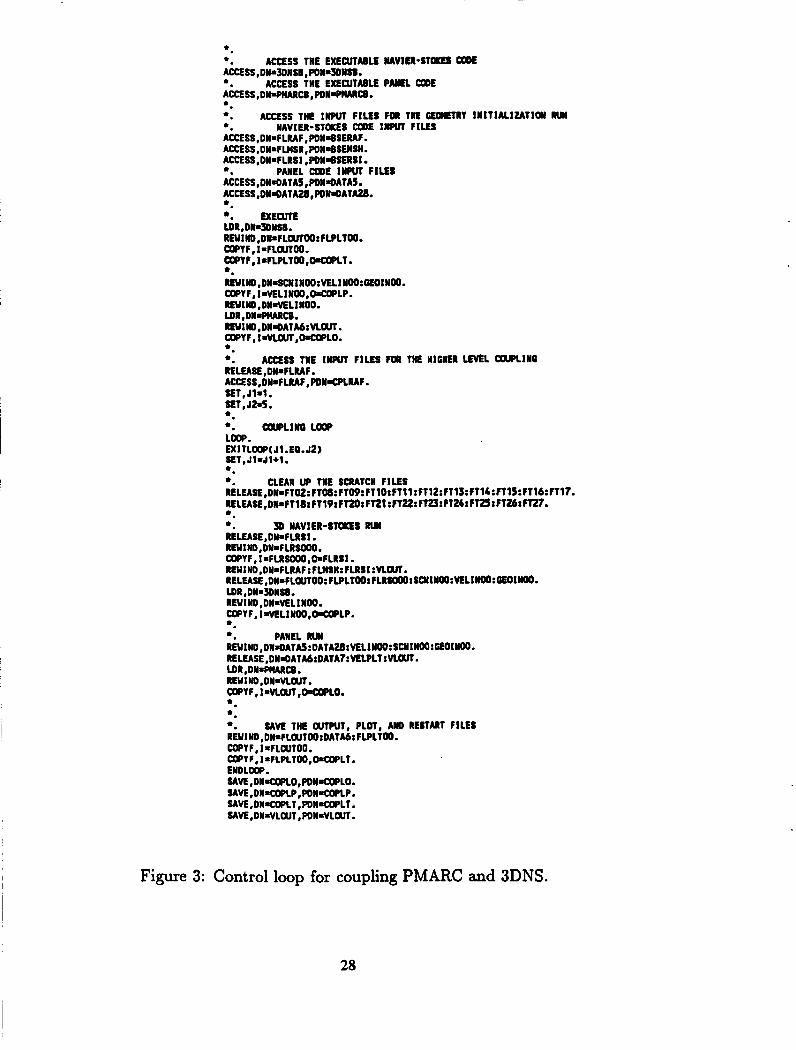
The interzone boundary surfaces are defined in the computational i j k space of the 3DNS grid by specification of ranges for the i , j , and k indicies. The type of interface boundary (e.g. PMARC boundary) is also specified in the input file. The boundaries can consist of more than one surface! to form a complex interzone boundary. On each surface one of the indices is assumed to be constant. For example, in Figure 2 the PMARC boundary is generated from two surfaces defined by the 3DNS grid. On one surface the j-index is constant, on the other the i-index is constant.

10

The panels defining the PMARC boundary are defined to coincide with the computational grid for the 3DNS code. This allows the coupling procedure to proceed without the need for interpolating the 3DNS solution on to the PMARC boundary. However, for complex flows an interpolation would provide more flexi- bility for positioning the PMARC boundary, The normal velocities for individual panels on this surface are calculated at the center of the panel using the 3DNS solution in the surrounding cells. The sign convention for the normal outward as positive in a right hand coordinate system for both codes results in the correct value for the normal velocity.

The 3DNS interzone boundary is specified in a like manner to the PMARC boundary. For this type of surface a file containing the locations of the boundary cell centers, at which the boundary condition information is required, are written to the file used by PMARC in the velocity scan routine.

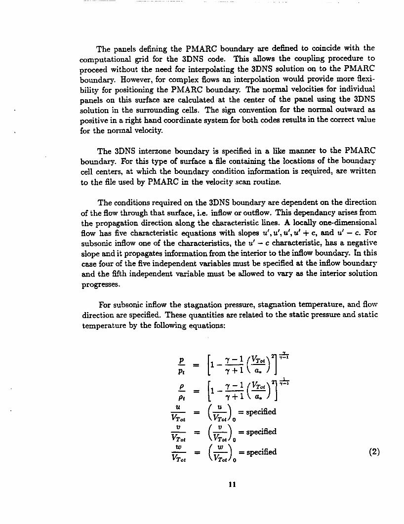
The conditions required on the 3DNS boundary are dependent on the direction of the flow through that surface, i.e. idow or outflow. This dependancy arises from the propagation direction along the characteristic lines. A locally one-dimensional flow has five characteristic equations with slopes u',u', u',u' + c, and u' - c. For subsonic inflow one of the characteristics, the u' - c characteristic, has a negative slope and it propagates information from the interior to the idow boundary. In this case four of the five independent variables must be specified at the inflow boundary and the fifth independent variable must be allowed to vary as the interior solution progresses.

For subsonic inflow the stagnation pressure, stagnation temperature, and flow direction are specified. These quantities are related to the static pressure and static temperature by the following equations:

Pt

Pt U - = (&)o = specified

VTot 2) - = (&)o = specified

VTot W - = (c)o = specified

VTot

11

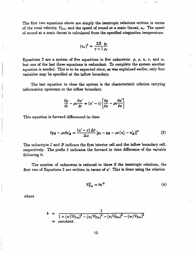
The first two equations above are simply the isentropic relations written in terms of the total velocity, and the speed of sound at a sonic throat, a,. The speed of sound at a sonic throat is calculated from the specified stagnation temperature.

2R pt (a*)2 = -- 7 + b t

Equations 2 are a system of five equations in five unknowns: p, p, u, v , and w, but one of the last three equations is redundant. To complete the system another equation is needed. This is to be expected since, as was explained earlier, only four variables may be specified at the inflow boundary.

The last equation to close the system is the characteristic relation carrying information upstream to the idow boundary.

s p 6u' 6Ut - -pcbt= bt (u' - 4 [$ - P C Z ]

This equation is forward differenced in time.

The subscripts I and B indicate the first interior cell and the inflow boundary cell, respectively. The prefix 6 indicates the forward in time difference of the variable following it.

The number of unknowns is reduced to three if the isentropic relations, the first two of Equations 2 are written in terms of u'. This is done using the relation

v;o* = buR

where

(4)

1 b = 1 + (u'/VTot)2 - (u/vTof)2 - (u /vTot )2 - (W/V*ot)*

= constant.

12

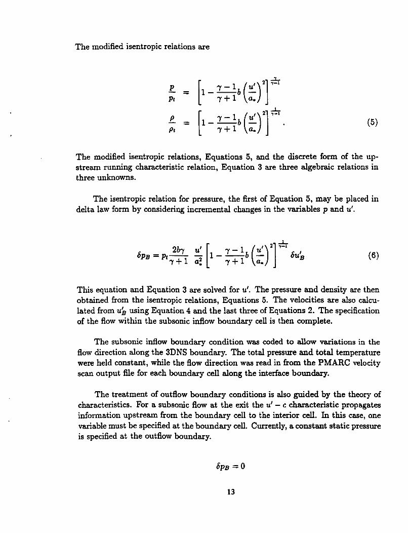
The modified isentropic relations are

1 7-1 u' - - P - ~---&(--)2]7-1-

Pt ( 5 )

The modified isentropic relations, Equations 5, and the discrete form of the upstream running characteristic relation, Equation 3 are three algebraic relations in three unknowns.

The isentropic relation for pressure, the first of Equation 5, may be placed in delta law form by considering incremental changes in the variables p and u'.

This equation and Equation 3 are solved for u'. The pressure and density are then obtained from the isentropic relations, Equations 5. The velocities are also calculated from ub using Equation 4 and the last three of Equations 2. The specification of the flow within the subsonic inflow boundary cell is then complete.

The subsonic inflow boundary condition was coded to allow variations in the flow direction along the 3DNS boundary. The total pressure and total temperature were held constant, while the flow direction was read in from the PMARC velocity scan output file for each boundary cell along the interface boundary.

The treatment of outflow boundary conditions is also guided by the theory of characteristics. For a subsonic flow at the exit the u' - c characteristic propagates information upstream from the boundary cell to the interior cell. In this case, one variable must be specified at the boundary cell. Currently, a constant static pressure is specified at the outflow boundary.

13

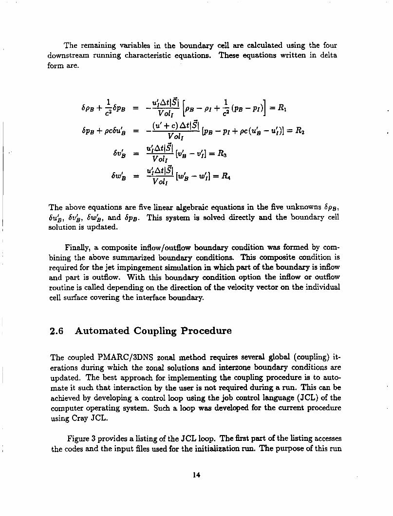
The remaining variables in the boundary cell are calculated using the four downstream running characteristic equations. These equations written in delta form are.

The above equations are five linear algebraic equations in the five unknowns 6 p ~ , 6uL, bvk, Sub, and 6 p ~ . This system is solved directly and the boundary cell solution is updated.

Finally, a composite inflow/outflow boundary condition was formed by com- bining the above summarized boundary conditions. This composite condition is required for the jet impingement simulation in which part of the boundary is inflow and part is outflow. With this boundary condition option the inflow or outflow routine is called depending on the direction of the velocity vector on the individual cell surface covering the interface boundary.

2.6 Automated Coupling Procedure

The coupled PMARC/3DNS zonal method requires several global (coupling) iterations during which the zonal solutions and interzone boundary conditions are updated. The best approach for implementing the coupling procedure is to auto- mate it such that interaction by the user is not required during a run. This can be achieved by developing a control loop using the job control language (JCL) of the computer operating system. Such a loop was developed for the current procedure using Cray JCL.

Figure 3 provides a listing of the JCL loop. The first part of the listing accesses the codes and the input files used for the initialization run. The purpose of this run

14

is for 3DNS to generate the interzone boundaries for PMARC and for PMARC to create an initial boundary condition file for 3DNS. The coupling loop is executed until the counter J1 reaches a preset limit 52. Before each code is m n during an iteration all unnecessary files are released and the input files and boundary condition files are rewound. After the code is run the data files that are accumulated for post-processing are copied to designated storage files. In the current loop the 3DNS code is run before PMARC. A similar procedure could have been developed to run PMARC first.

15

3 Test Cases

3.1 Coupled PMARC/3DNS Cases

To investigate the coupling of PMARC and 3DNS several test cases were run. The test cases were designed to be simple enough to allow the various coupling parameters to be studied efficiently.

3.1.1 Axisymmetric Jet

An axisymmetric jet in a coflowing stream provides a geometrically and numerically simple flow field, which is ideal for parametrically studying the coupling of PMARC and 3DNS. Physically, the important mechanism by which a viscous flow region can influence a potential flow region is through entrainment. The axisymmetric jet entrains mass from the coflowing streams as the jet develops downstream.

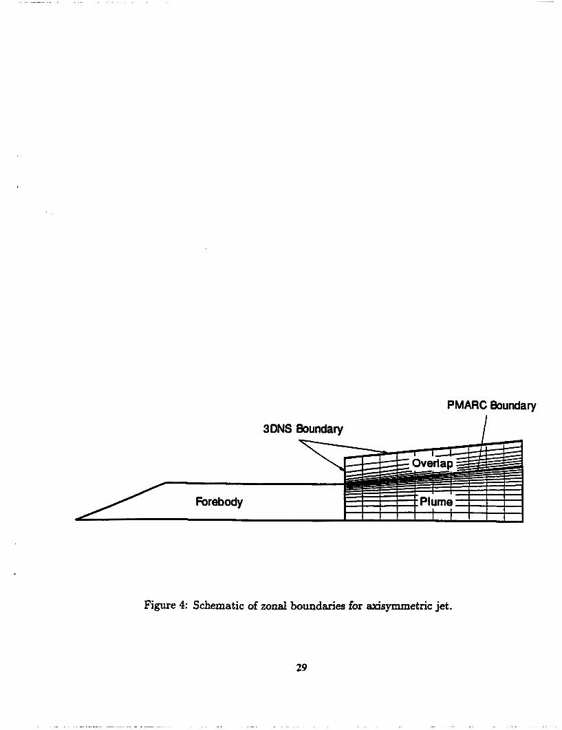
Figure 4 provides a schematic of the flow fieId under consideration. The forebody consists of a cylinder with a conical nose. The purpose of the forebody is to hold the nozzle and straighten the external flow to be parallel to the axis as it approaches the nozzle exit plane. The plume zone includes the complete computational grid used for the 3DNS analysis. The edge of the calculated jet shear layer is below the grid line designated as the PMARC boundary. This grid line attaches to the edge of the nozzle and is specified as part of the grid generation procedure. The 3DNS boundary is also specified as a means of controling the extent of the overlap region, which consists of the computational grid between the 3DNS and PMARC boundaries.

The Mach numbers of the jet and freestream were 0.9 and 0.3, respectively, for all calculations. Even though the flow field was axisymmetric, the calculations were run 3D.

Three patches were used to set up the panels for the PMARC calculations. The forebody patch consisted of 48 panels. The PMARC boundary patch panels were formed from the corresponding grid points in the plume zone. The third patch was a cap that closed the paneled configuration at the end of the PMARC boundary.

The goal of this study was to determine the effect of the overlap region and

16

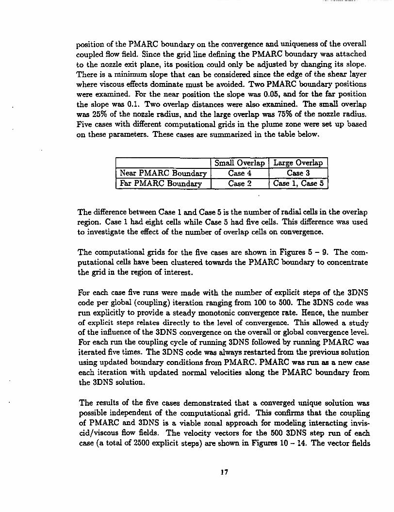
position of the PMARC boundary on the convergence and uniqueness of the overall coupled flow field. Since the grid line defining the PMARC boundary was attached to the nozzle exit plane, its position could only be adjusted by changing its slope. There is a minimum slope that can be considered since the edge of the shear layer where viscous effects dominate must be avoided. Two PMARC boundary positions were examined. For the near position the slope was 0.05, and for the far position the slope was 0.1. Two overlap distances were also examined. The small overlap was 25% of the nozzle radius, and the large overlap was 75% of the nozzle radius. Five cases with different computational grids in the plume zone were set up based on these parameters. These cases are summarized in the table below.

Small Overlap Large Overlap Near PMARC Boundarv Case 4 - , I Far PMARC Boundary I Case 2 I Case 1, Case 5

Case 3

The difference between Case 1 and Case 5 is the number of radial cells in the overlap region. Case 1 had eight cells while Case 5 had five cells. This difference was used to investigate the effect of the number of overlap cells on convergence.

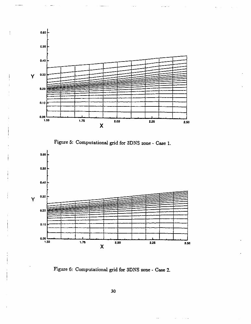
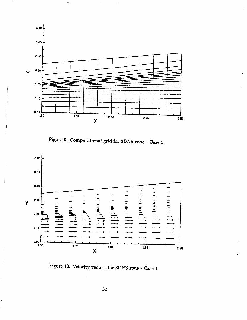
The computational grids for the five cases are shown in Figures 5 - 9. The computational cells have been clustered towards the PMARC boundary to concentrate the grid in the region of interest.

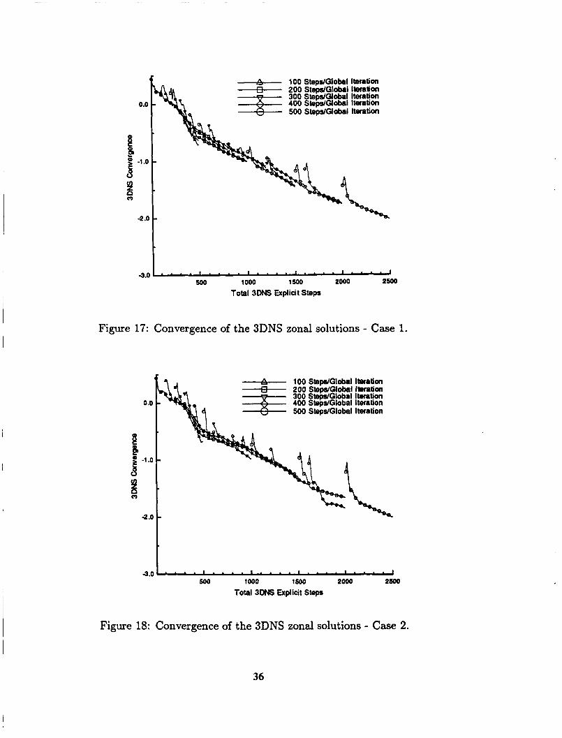
For each case five runs were made with the number of explicit steps of the 3DNS code per global (coupling) iteration ranging from 100 to 500. The 3DNS code was run explicitly to provide a steady monotonic convergence rate. Hence, the number of explicit steps relates directly to the level of convergence. This allowed a study of the influence of the 3DNS convergence on the overall or global convergence level. For each run the coupling cycle of running 3DNS followed by running PMARC was iterated five times. The 3DNS code was always restarted from the previous solution using updated boundary conditions from PMARC. PMARC was run as a new case each iteration with updated normal velocities along the PMARC boundary from the 3DNS solution.

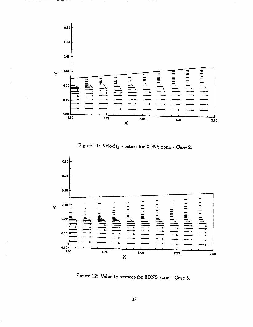
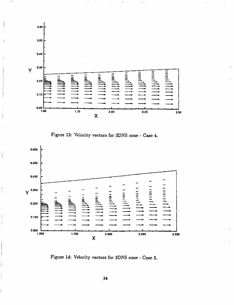
The results of the five cases demonstrated that a converged unique solution was possible independent of the computational grid. This confirms that the coupling of PMARC and 3DNS is a viable zonal approach for modeling interacting inviscid/viscous flow fields. The velocity vectors for the 500 3DNS step run of each case (a total of 2500 explicit steps) are shown in Figures 10 - 14. The vector fields

17

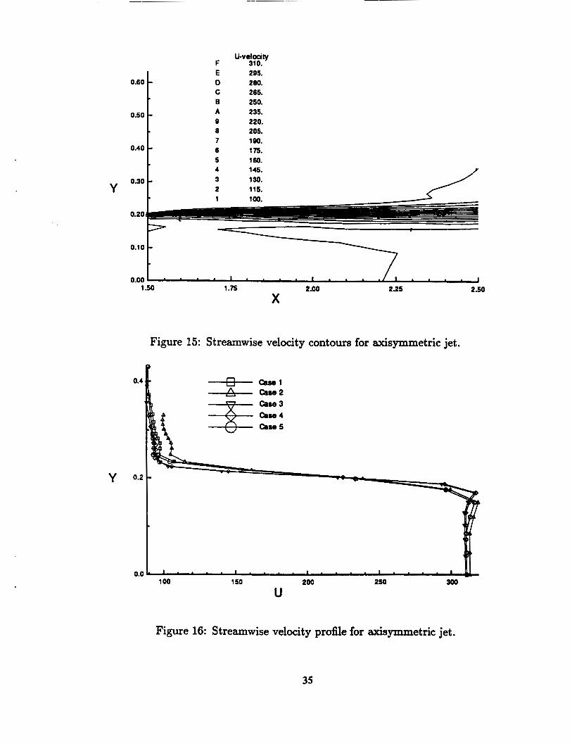
are consistent for each case. Figure 15 provides contours of the streamwise velocity component indicating the development of the shear layer. Figure 16 shows the velocity profile at x = 2.3, which demonstrates that all cases have converged to the same solution. The differences in the thickness of the shear layer are due to the different grid resolutions. Case 2 shows some irregukmties in the vicinity of the freestream, which may be related to the grid which was not one that typically would be chosen.

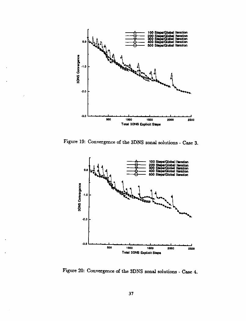
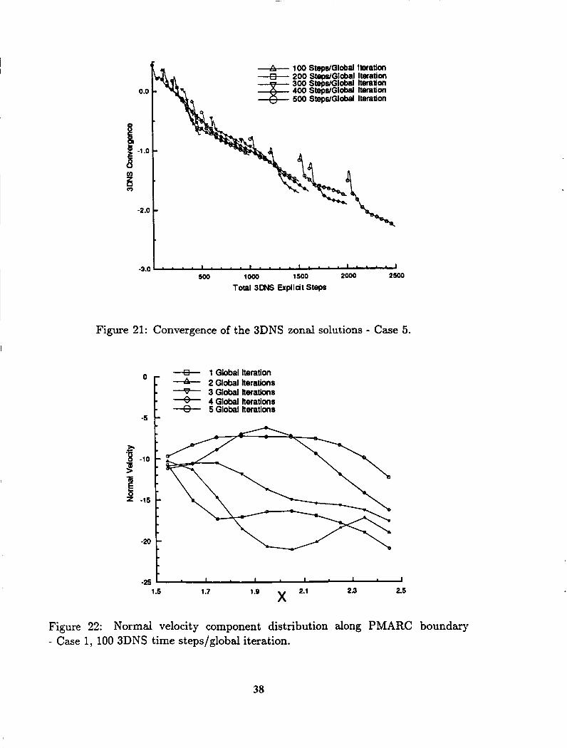
Convergence of the zonal solutions is necessary in order to achieve convergence of the overall solution. PMARC was allowed to converge to a very low level each global (coupled) iteration, because it was not possible to restart the solution from a previous run. This was not detrimental for the current investigation since the total number of panels and, therefore, run times were small. For cases with large numbers of panels it may be advantageous to only converge PMARC to a level comparable to the convergence of the boundary conditions since they govern the convergence of the overall solution. The 3DNS calculations were substantially more expensive than PMARC. Therefore, it was not reasonable to converge the 3DNS solution to a low level each global iteration. Figures 17 - 21 provide the 3DNS solution convergence histories for the five runs of each case. Clearly, each case is convergent. As can be seen, the convergence is basically monotonic and the level of convergence of the 3DNS solution is directly related to the total number of explicit steps. A noticeable feature is the abrupt spikes that occur as the 3DNS solution is restarted each global iteration. They are a result of the updated 3DNS boundary conditions after each PMARC run. The spikes are mostly short-lived and do not seem to significantly influence the convergence path. The spikes appear to be large when the overlap is small and when the PMARC boundary is near to the shear layer. The level of convergence is best when the overlap is large (Cases 1, 3 and 5). The greater distance probably allows the perturbations generated at the boundaries to dissipate more before reaching the PMARC boundary where they can be fed back into the PMARC solution. The convergence path also appears to be influenced by the overlap. The small overlap (Cases 2 and 4) and the large overlap with fewer cells (Case 5 ) show more of a spread in the convergence paths. This again may result from less dissipation of perturbations and a feedback with the outer boundary.

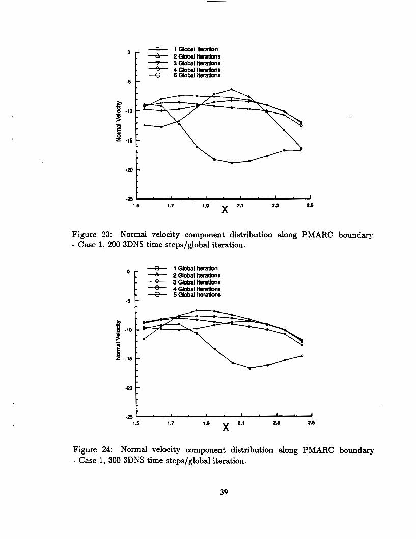
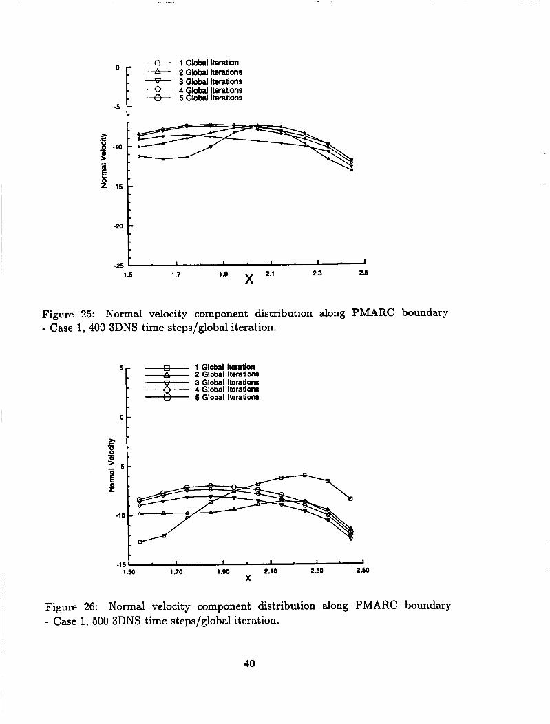
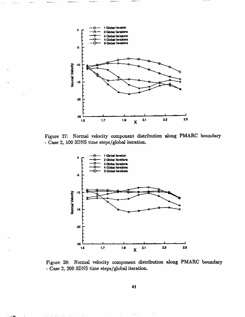
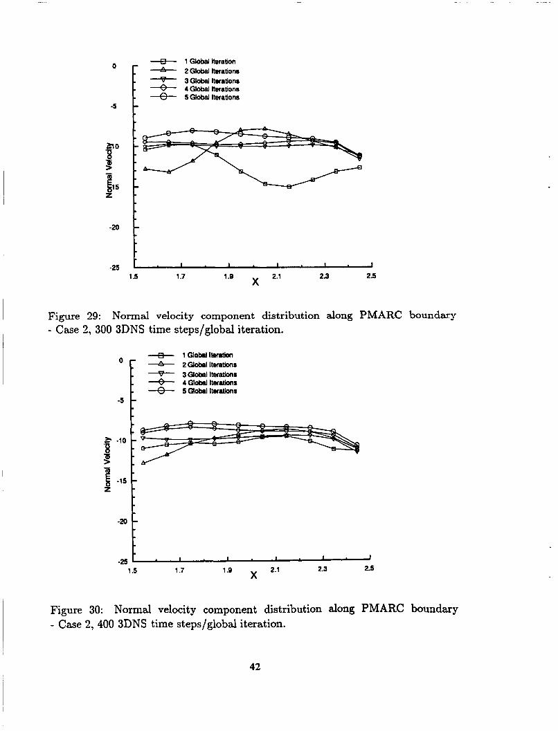
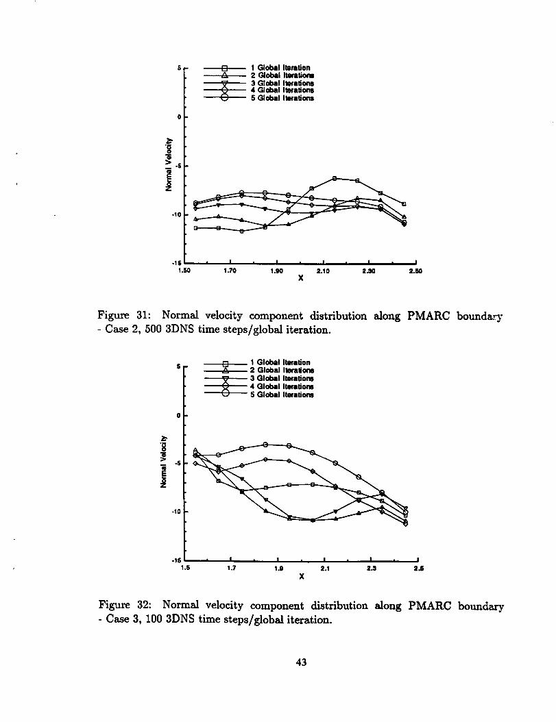
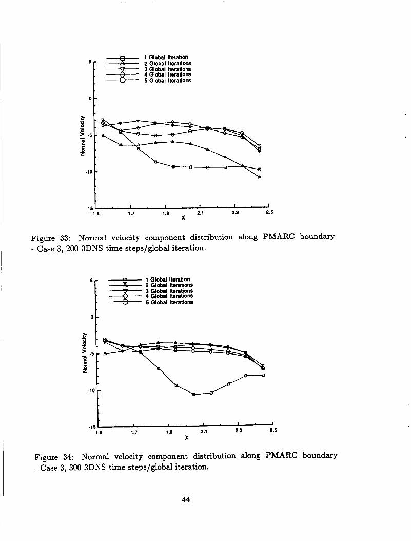
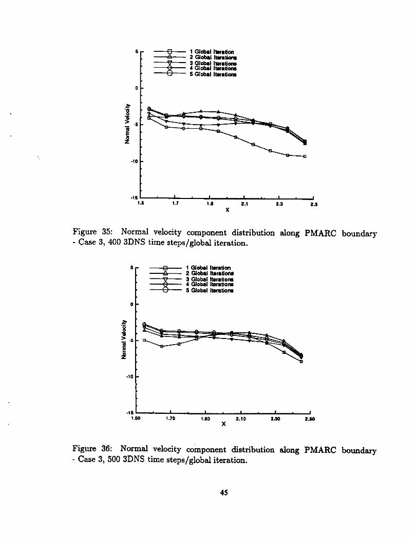
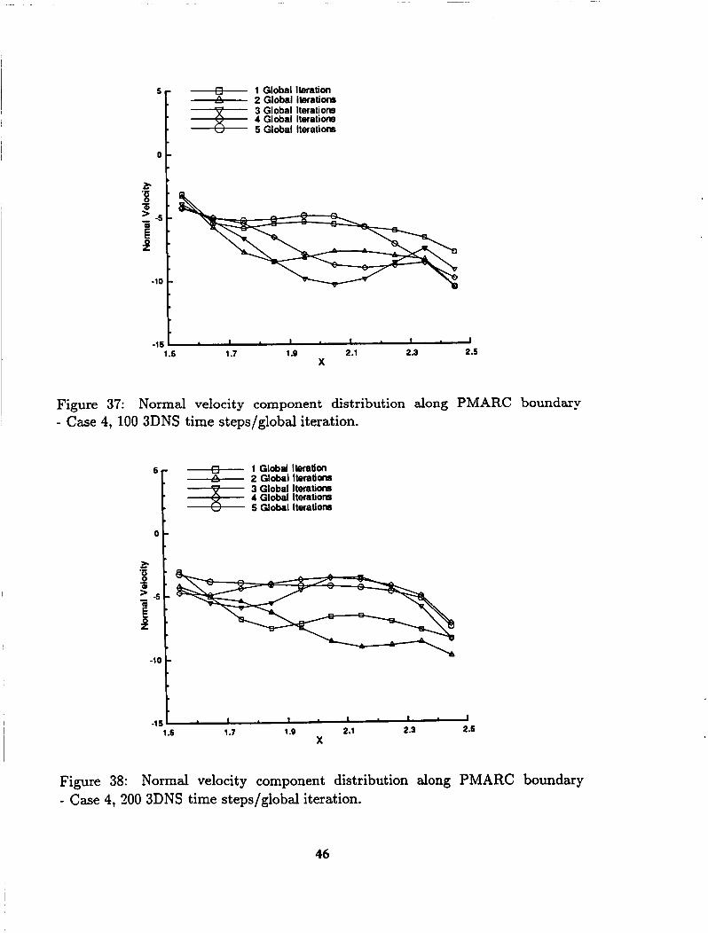
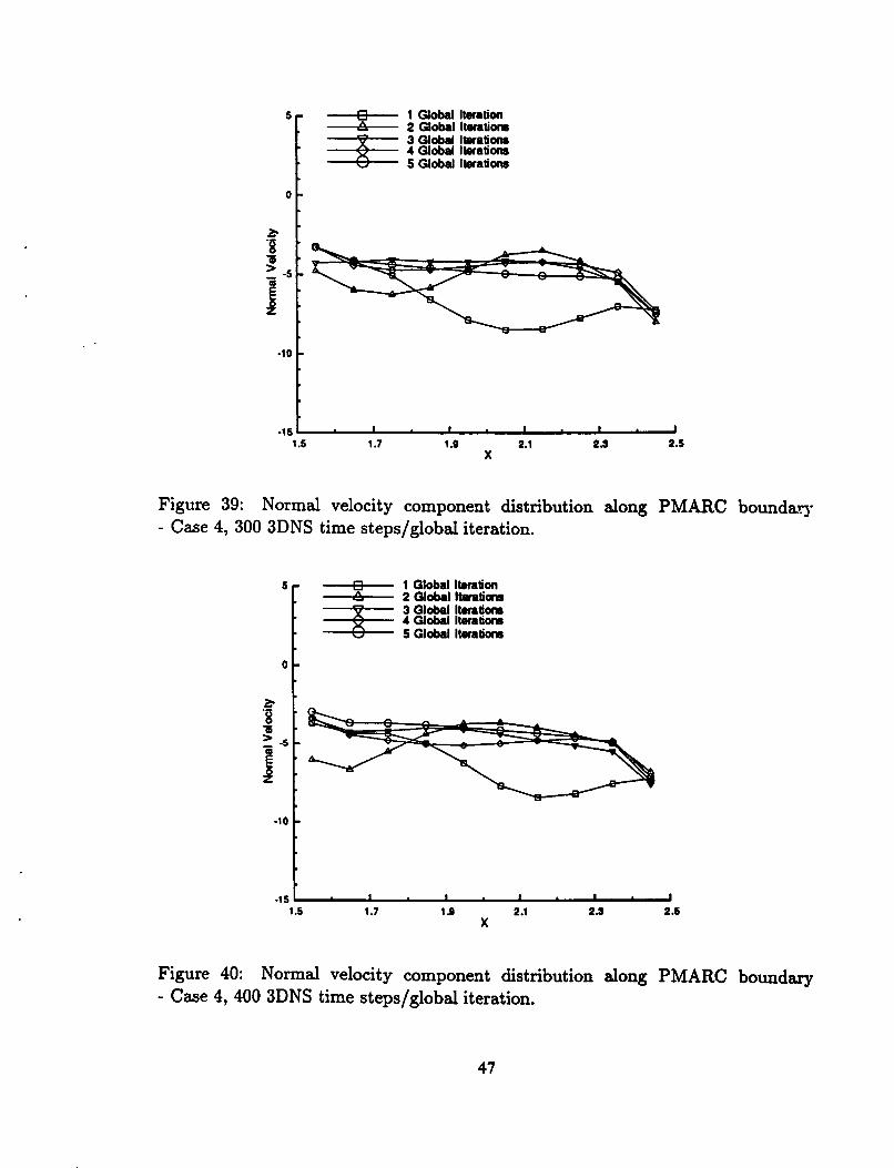
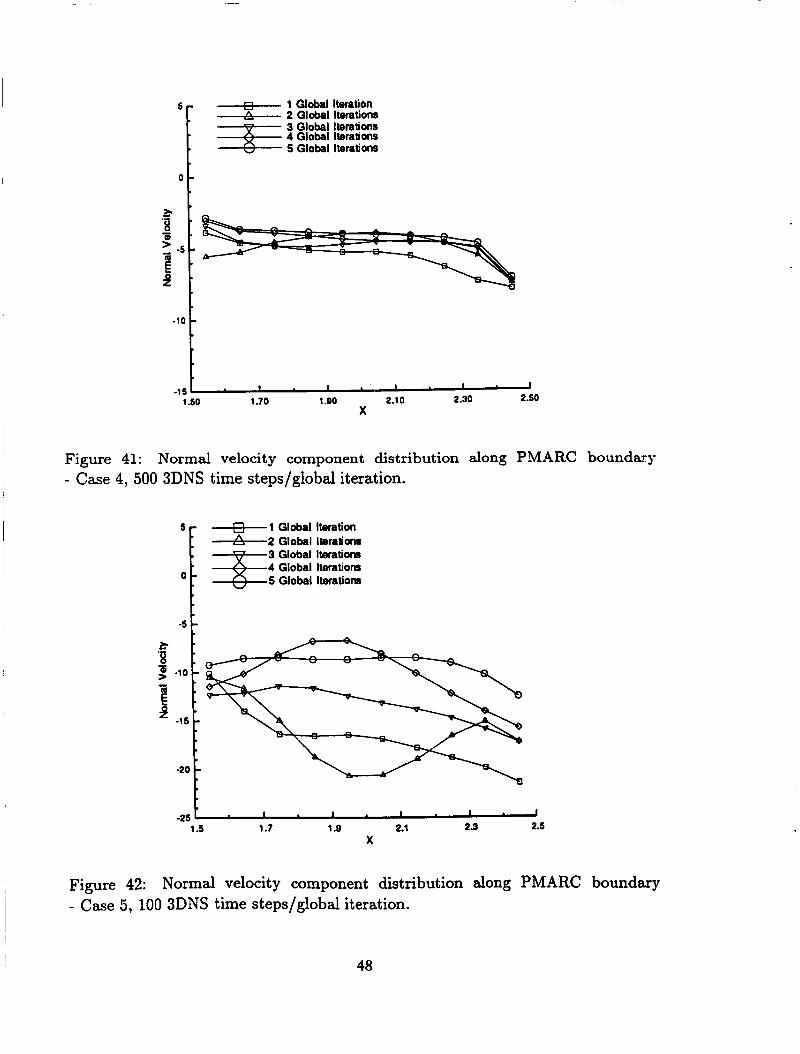
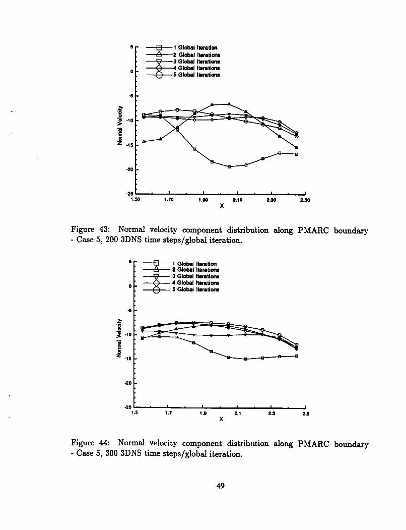
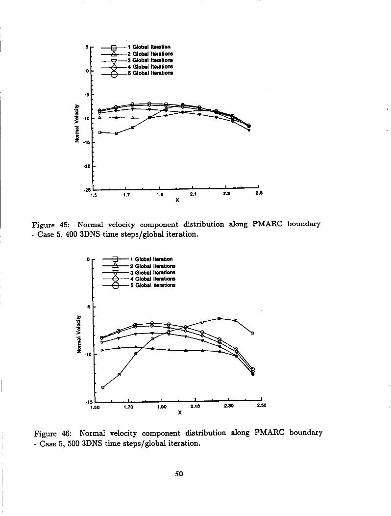
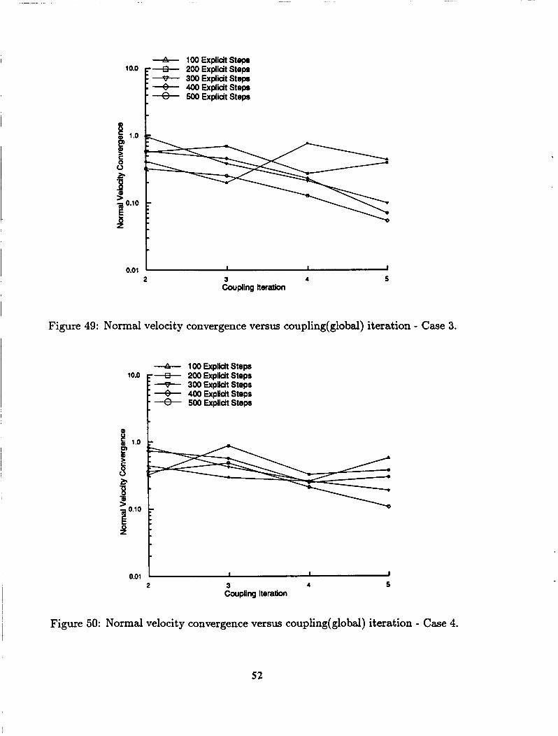
The convergence of the normal velocities on the PMARC boundary is directly indica- tive of the convergence of the overall solution. Figures 22 - 46 provide distributions of the normal velocity along the PMARC boundaries for each global iteration for each run of each case. A survey of these figures leads to the obvious conclusion that more explicit steps of the 3DNS code per global iteration results in better convergence of the normal velocities. However, the situation is not always that simple, particularly when the cost effectiveness of a coupled analysis is considered.

18

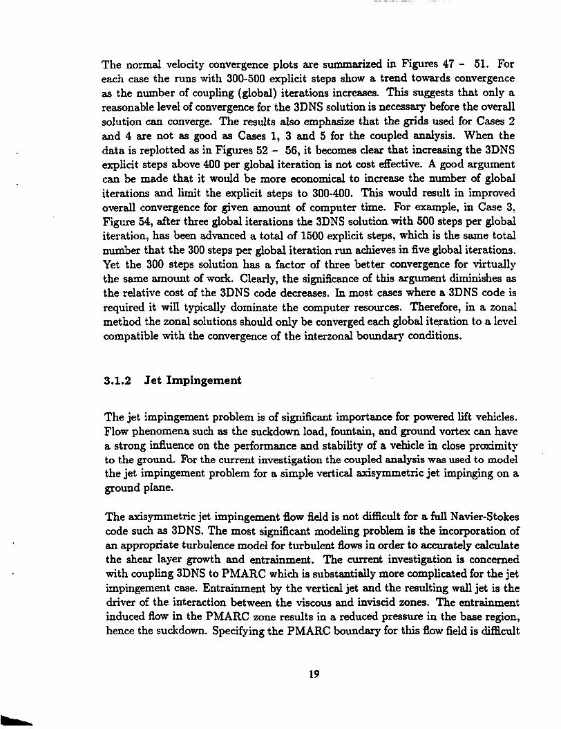
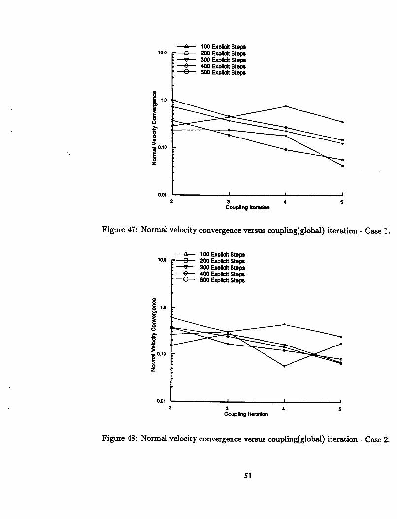
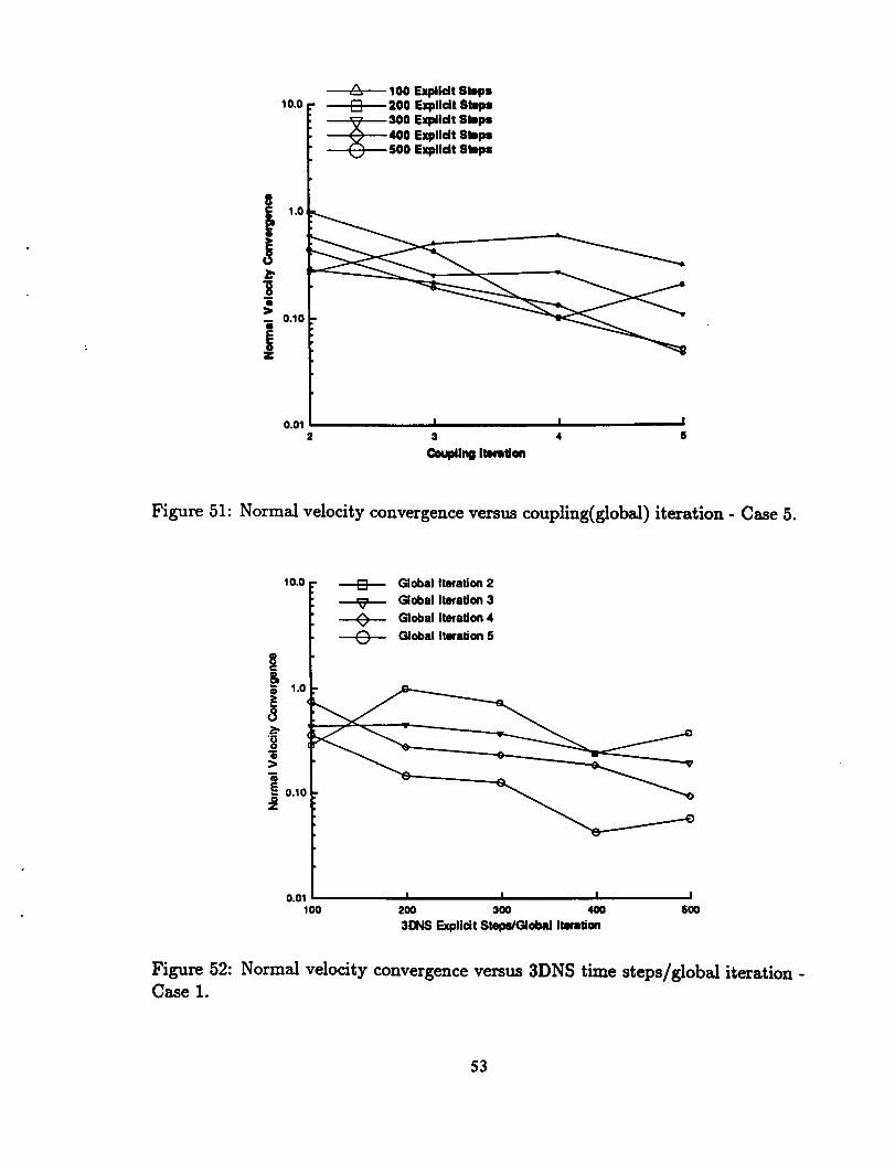
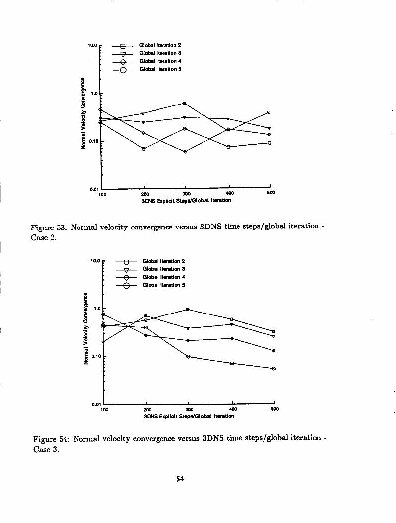
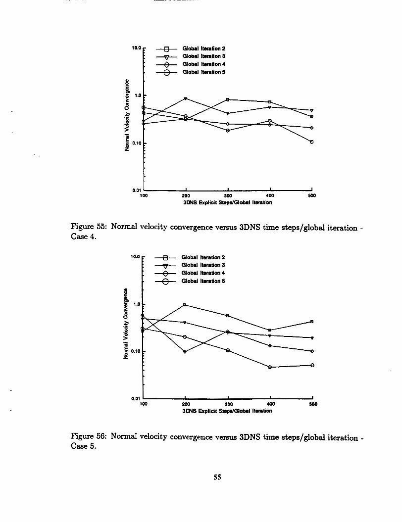
The normal velocity convergence plots are summarized in Figures 47 - 51. For each case the runs with 300-500 explicit steps show a trend towards convergence as the number of coupling (global) iterations increases. This suggests that only a reasonable level of convergence for the 3DNS solution is necessary before the overall solution can converge. The results also emphasize that the grids used for Cases 2 and 4 are not as good as Cases 1, 3 and 5 for the coupled analysis. When the data is replotted as in Figures 52 - 56, it becomes clear that increasing the 3DNS explicit steps above 400 per global iteration is not cost effective. A good argument can be made that it would be more economical to increase the number of global iterations and limit the explicit steps to 300-400. This would result in improved overall convergence for given amount of computer time. For example, in Case 3, Figure 54, after three global iterations the 3DNS solution with 500 steps per global iteration, has been advanced a total of 1500 explicit steps, which is the same total number that the 300 steps per global iteration run achieves in five global iterations. Yet the 300 steps solution has a factor of three better convergence for virtually the same amount of work. Clearly, the significance of this argument diminishes as the relative cost of the 3DNS code decreases. In most cases where a 3DNS code is required it will typically dominate the computer resources. Therefore, in a zonal method the zonal solutions should only be converged each global iteration to a level compatible with the convergence of the interzonal boundary conditions.

3.1.2 Jet Impingement

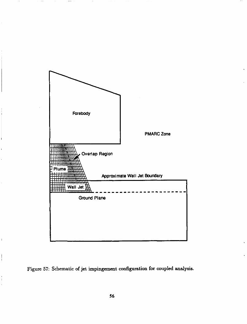
The jet impingement problem is of significant importance for powered lift vehicles. Flow phenomena such as the suckdown load, fountain, and ground vortex can have a strong influence on the performance and stability of a vehicle in close proximity to the ground. For the current investigation the coupled analysis was used to model the jet impingement problem for a simple vertical axisymmetric jet impinging on a ground plane.

The axisymmetric jet impingement flow field is not difficult for a full Navier-Stokes code such as 3DNS. The most significant modeling problem is the incorporation of an appropriate turbulence model for turbulent flows in order to accurately calculate the shear layer growth and entrainment. The current investigation is concerned with coupling 3DNS to PMARC which is substantially more complicated for the jet impingement case. Entrainment by the vertical jet and the resulting wall jet is the driver of the interaction between the viscous and inviscid zones. The entrainment induced flow in the PMARC zone results in a reduced pressure in the base region, hence the suckdown. Specifying the PMARC boundary for this flow field is difficult

19

due to the presence of the wall jet. It is not possible to include the actual ground plane in the PMARC boundary, since that would assume that PMARC could model the wall jet. The PMARC boundary must be positioned above the shear layer associated with the wall jet where the only influence results from entrainment by the walljet. The current approach is shown schematically in Figure 57. A segment of the PMARC boundary is positioned along the vertical jet using the same approach as in the axisymmetric jet case. Similarly, a mesh plane (with a constant I-index) is chosen to form the segment of the PMARC boundary above the wall jet. The normal velocities are directly obtained from the SDNS solution. This segment of the PMARC boundary is extended beyond the 3DNS zone as a wall. The configuration is capped-off by segments that form a finite thickness cylinder.

The radius and thickness of the cylinder had a profound influence on the PMARC solution in the overlap region. This was most likely due to the corner flow at the edge of the cylinder. To minimize this influence, several runs were made with the basic configuration at a freestream Mach number of 0.003 while varying the radius and thickness of the cylinder. The results of this study indicated that by increasing both the disk radius and thickness to 12 times the nozzle radius the iduence became negligible.

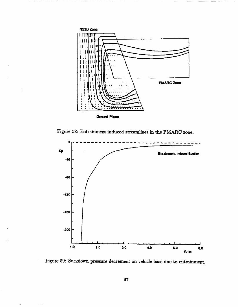
The 3DNS flow field solution created an entrainment of the surrounding fluid in the PMARC zone. Since the entrained flow must pass between the lower boundary and the base of the vehicle, it will accelerate to a velocity greater than the freestream. Figure 58 shows a set of streamlines passing through the PMARC zone and into the jet. The increased velocity of the entrained flow lowers the pressure on the base of the vehicle creating the suckdown load. Figure 59 provides a plot of the pressure from the PMARC solution along the radius of the base, which shows the pressure decreasing as the vertical jet is approached. This coupled solution shows how the interaction of a limited viscous zone with the surrounding inviscid zone can provide an overall flow solution that can be used to determine the loads on a powered-lift aircraft while minimizing the computational expense.

3.2 SDNS to SDNS Coupling

The geometries of 3D powered lift configurations will have viscous flow regions that can not be readily modeled using one zone due to grid generation considerations. These regions may include complex inlets, nozzles, ducts, flaps, separated flow, etc. To simplify the grid generation process it is often convenient to divide the region into severd connected viscous zones which must then be coupled by the solution

20

procedure. This coupling is straight forward since the boundary conditions are directly compatible at the interzonal boundaries.

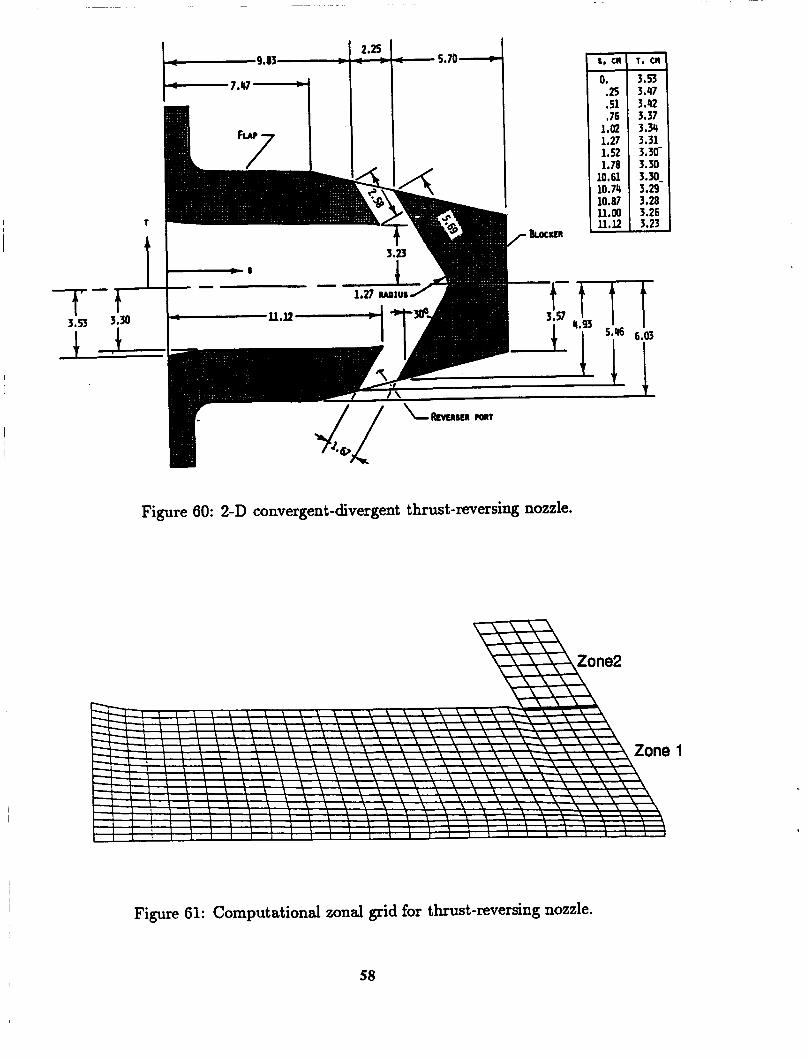
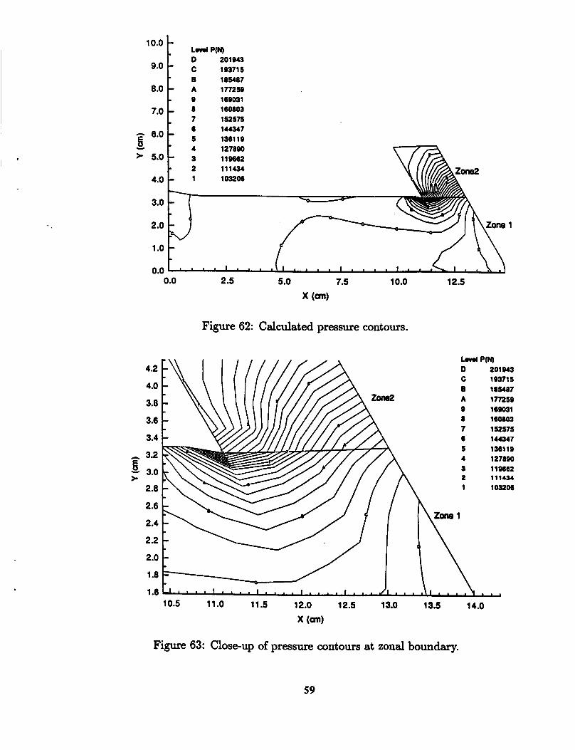
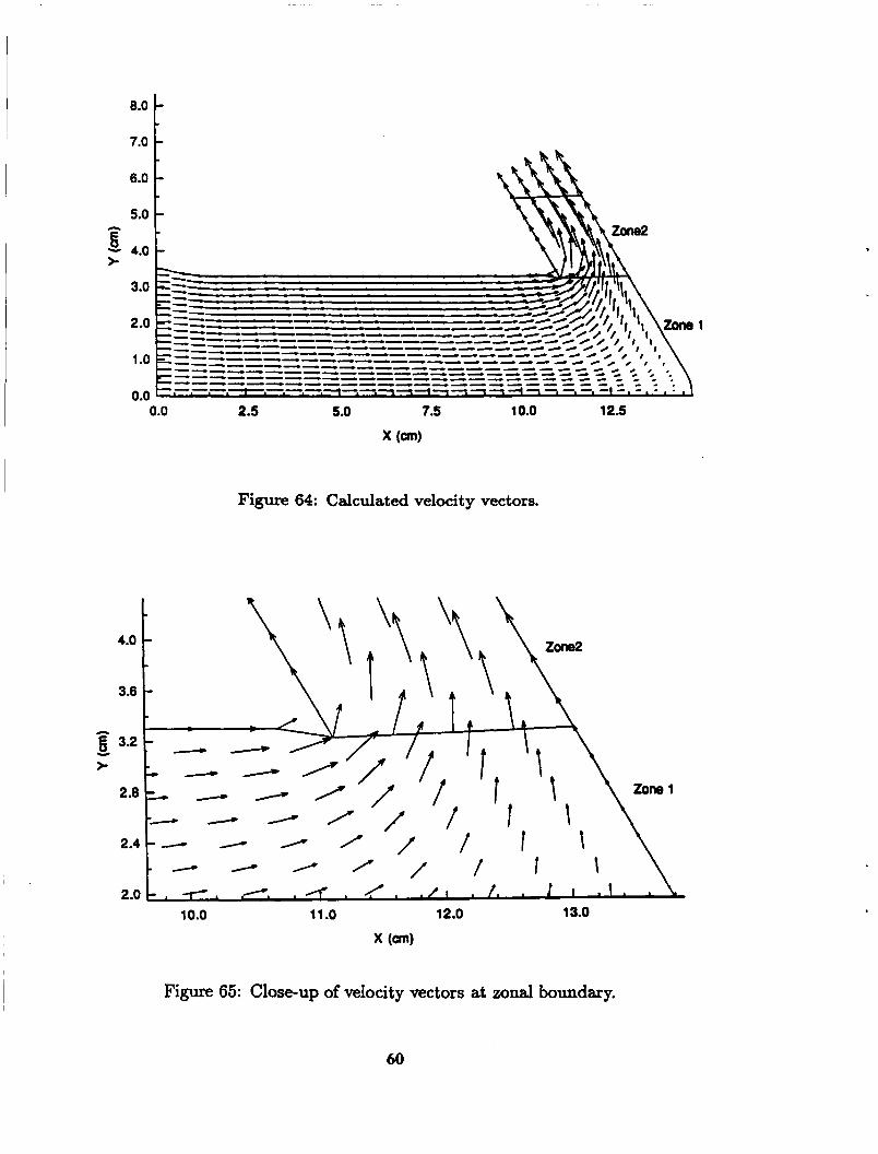
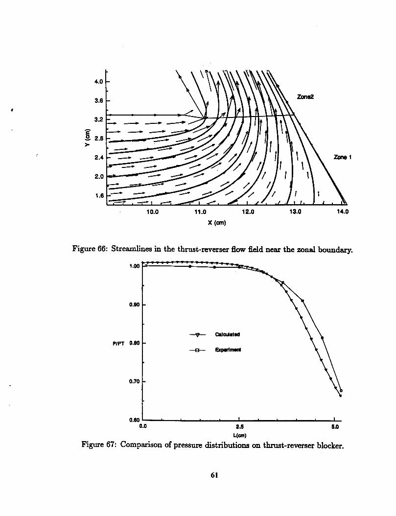
The 3DNS code has the capability to couple multiple zones. To demonstrate this feature a thrust reversing nozzle, Figure 60, flow field was calculated. The geometry was divided into two zones to generate the computational grid as shown in Figure 61. The grid was 3D, but just five cells were used in the %direction. The 3DNS solution was run by advancing the solution one time step in each zone, updating the interzone boundary conditions, then repeating the process. The solution was run 3500 steps at which the residuals had been reduced by approximately five orders of magnitude. The primary concern for this case was verifying the continuity of the solution across the interzone boundary. Figure 62 shows the pressure contours for both zones. A close examination, Figure 63, reveals that the contour lines are smooth and continuous across the boundary. Figures 64 and 65 provide the velocity vectors which do not show any irregularities. Streamlines in the vicinity of the interzone boundary are presented in Figure 66. Again, the streamline trajectories at the boundaries are smooth. The calculated pressure distribution along the internal wall of the blocker is compared with the available experimental data [26] in Figure 67. The agreement is quite reasonable, particularly in consideration of the very coarse mesh in the reverser port.

This case has demonstrated that the coupling of multiple 3DNS zones is operational and provides consistent solutions at the interzone boundaries.

21

4 Conclusions

As a result of the work reported here several conclusions can be made. These are enumerated below.

1. The zonal method based on the coupling of a 3D Navier- Stokes code, 3DNS, to a panel method potential flow code, PMARC, has been demonstrated to provide unique and convergent overall solutions, which make it a viable flow analysis tool.

2. The test cases indicate that a large overlap of the interzone boundaries yields faster convergence rates for the overall solution.

3. The cost effectiveness of the coupled analysis is enhanced if the zonal solutions are converged simultaneously with the interzone boundaries instead of converging them to arbitrarily low levels. In other words the zonal solutions should not be converged faster than the overall solution.

4. The jet impingement case demonstrated the effectiveness of the zonal method for modeling the influence of a viscous zone on the flow field around a vehicle.

5. The 3DNS to 3DNS coupling demonstrated the usefulness of multiple viscous zones for modeling geometrically complex flows.

22

5 Recommendations

The following recommendations are made to encourage the development of the zonal method.

1. The turbulence model in 3DNS should be upgraded to a more general model that can accurately simulate the turbulence of curved shear layers. This is of great importance for powered- lift flow fields.

2. An adaptive grid utility that would automatically adjust the 3DNS grid based on the positions of the shear layers would enhance the accuracy and cost effectiveness of the zonal method.

3. The PMARC boundary position should be made independent of the 3DNS grid lines. This would require the addition of a 3D interpolator to obtain the normal velocities from the 3DNS solution.

4. The coupling procedure should be optimized by forcing both the PMARC and 3DNS zonal solutions to automatically converge simultaneously with the interzone boundary conditions.

5. Numerous test cases for different powered-lift flows should be run and compared with experimental data.

23

References

[l] Richey, G.K. and Campbell, D.J., “Air Force Views on Technology Needs for V/STOL Tactical Fighter Aircraft,” Tactical Aircraft Research and Technol- ogy, Vol. I, NASA CP 2162, Part 1, 1981, p.45.

[2] Bowers, D.L. and Laughrey, J.A., ”Advanced Exhaust Nozzles for Tactical Aircraft,” Tactical Aircraft Research and Technology, Vol. I, NASA CP 2162, Part 2, 1981, p. 633.

[3] Lind, G.W. and Tamplin, G., “V/STOL Technology Requirements for Future Fighter Aircraft ,” AIAA Paper No. 81-1360,17th Joint Propulsion Conference, July 1981.

[4] Capone, F.J., Hunt, B.L., and Poth, G.E., “Subsonic/Supersonic Nonvectored Aeropropulsive Characteristic of Nonaxisymmetric Nozzles Installed on an F- 18 Model,” AIAA Paper No. 81-1445, 17th Joint Propulsion Conference, July 1981.

[5] Paulson, J.W., “Thrust-Induced Aerodynamics of STOL Fighter Confipprii- tions,” Tactical Aircraft Research and Technology Vol. I, NASA CP 2162, Part 2, 1981, p. 695.

[6] Sheridan, -4.E., “Turbine Bypass Remote Augmentor Lift System for V/STOL Aircraft,” AIAA Journal of Aircraft, Vol. 23, No. 9, Sept. 1986, pp 703-710.

(71 Williams,J. Butler,S.F.J., and Wood,M.N., “The Aerodynamics of Jet Flaps,” RAE RStM No. 3304, Jan 1961.

[8] I(rothapal1i.A. and Leopold,D., “Effects of a Ground Vortex on the Aerody- namics of an Airfoil,” NASA Conference Publ. 10008, 1987 Ground Vortez Workshop, edited by Margason,R.J., April 1987.

(91 Kuhn,R.E., “V/STOL Ground Effects and Testing Techniques, Flow Field In- vestigation,” NASA Conference Publ. 2462, 1985 NASA Ames Research Cen- ter’s Ground-Effects Workshop, edited by Mithcell,K., August 1985.

[lo] Roherts,D.W., “Prediction of Subsonic Aircraft Flows with Jet Exhaust In- teractions,” AGARD Confer. Proc. No. 301, Aerodynamics of Power Plant Installations, May 1981, Toulouse, fiance.

(111 Roherts,D.lV., “A Zonal Method for Modeling 3-D Aircraft Flow Fields With Jet Plume Effects,” AIAA Paper No. 87-1436, 1987.

24

[ 121 Lemmerman, L.A. and Sonnad, V.R., "ThreeDimensional Viscous-Inviscid Coupling Using Surface Transpirational," Journal of Aircrajl, Vol. 16, No. 6? June 1979, pp353.

[13] Brune, G.N., Rubbert, P.E., and Forester, C.K., "The Analysis of Flow Fields with Separation by Numerical Matching," Symposium on Flow Separation, AGARD Fluid Dynamics Panel, 27-30, May 1975, Gottingen, Federal Republic of Germany.

[14] Putnam, L.E. and Hodges, J., "Assessment of NASA and RAE Vis- cous/Inviscid Interaction Methods for Predicting Transonic Flow Over Nozzle Afterbodies," AIAA Paper 83-1789, July 1983.

[15] Dash, S.M., Wihouth, R.G. and Pergament, H.S., "An Overlaid Vis- cous/Inviscid Model for the Prediction of Nearfield Jet Entrainment," AIAA Journal, Vol. 17, September 1979, pp950-958.

[16] Mahgoub, H.E.H. and Bradshaw, P., "Calculation of Turbulent-Inviscid Flow Interactions with Large Normal Pressure Gradients." AIAA Journal, pp1025- 1029, October 1979.

[17] Dash, S.M., "Recent Developments in the Modeling of High Speed Jets, Plumes, and Wakes," AIAA Paper 85-1616, July 1985.

[IS] Anderson, D. A. , Tannehill, J. C. , and Pletcher, R. H. Computational Fluid Mechanics and Heat l'kansfer, McGraw-Hill, 1984.

[19] Peery, K.M. and Imlay, S.T., "An Efficient Implicit Method for Solving Viscous Multi-Stream Nozzle/Afterbody Flow Fields," AIAA Paper No. 86-1380, June 1986.

[20] MacCormack, R. W., "Current Status of Numerical Solutions of the Navier- Stokes Equations," AIAA Paper No. 85-0032, Jan. 1985.

Navier-Stokes Equations," AIAA Paper No. 85-150, July 1985.

ization," AIAA Paper No. 840165, Jan. 1984.

[21] Thomas, J.L., and Walters, R.W., "Upwind Relaxation Algorithms for the

[22] Chakravarthy, S.R., "Implicit Upwind Schemes Without Approximate Factor-

[23] Steger, J.L. and Warming, R.F., "Flw Vector Splitting of the Inviscid Gasdy- namic Equations with Applications to Finite- Difference Methods," Journal of C O ~ P . Phys., Vol. 40, pp 263-293, 1981.

[24] Roe, P.L., "Approximate Riemann Solvers, Parameter Vectors, and Difference Schemes," Journal of Computational Physics, Vol. 43, 1981, pp. 357-372.

25

[25] Baldwin, B. and Lomax, H., "Thin-Layer Appraximation and Algebraic Model for Separated Turbulent Flows,'' AIAA Paper No. 78-257, Jan. 1978.

[26] Putnam, L.E. and Strong, E.G., "Internd Pressure Distributions for a Two- Dimensional Thrust-Reversing Nozzle Operating at a Ree-Stream Mach Num- ber of Zero," NASA TM85655, December 1983.

26

PMARC ZONE

Coi nci dent Interzone Boundaries

3DNS Boundary Cells /

_ _ _ - _ - - - - - - - - - - _ _ _ _ _ _ _ _ _ _ - - - - - - - - Effective Overlap

Location of Flow Vari ab1 es

3DNS ZONE

Figure 1: Half cell overlap when interzone boundaries coincide.

Figure 2: PMARC boundary formed from two grid surfaces in the 3DNS zone.

27

*. *. ACCESS THE EXECUTMLE NAVIER-STmt ACCESS,DH~U)HSB~ PDW~U)RSB. *. ACCESS,DNIPIIARCB, PDHrpIuRcS. *. *. *. WAVIER-STOIES CODE INPUT FILES

ACCESS,DW=FUISH,PDH4S~SH.

*. PANEL CODE lWPUT FILES ACCESS,DH.DATAS ,PDWI)ATAS. ACCESS,DW.DATAZ8, PDH.OATA28. *. *. EXECUTE lDR,DH=U)HSB. REWI ND ,DH=FLOUTOO: FLPLTW. COPYF, I-FLOUTOO. COPY F, I=FLPLTW ,OICQPM. *. REWIND ,DW=StW1100:VELl W O O :GEOIYW. COPYF,I=VELIHW,O=CWLP. REWIND,DW=V€LIHOO. lDR ,DH.#URCB. REWIND ,DN.DATA6:VLOUT. QIPYF,I=VLOUT,O=CWLO. *. *. RELEASE,DN=FLRAF. ACCESS ,DH=FLRAF, PDW4PLRAF.

SET,J2.5. *. *. COUPLIHO LOOP LOOP. E)( I TLOOPC J 1 .EO. JZ) SET,Jl=Jl+l. *.

ACCESS THE EXECUTABLE PAMEL COOE

ACCESS THE I W FILES FOR THE GECUETRY I N I T I A L I U T I Q ( RUN

ACCESS,DH=FLRAF ,PDW4SERAF.

ACCESS,DW=FLRSI ,PDH#QRSl

ACCESS THE INPUT FILES FOR THE HIGHER LEVEL COUPLIHO

m,~i=i.

*. RELEASE .DW=FTOZ: FTOB: FTO9: FT10: f 11 1 : f 112: FT13:FT14: FTlS: FT16: FTl7.

CLEAR UP THE SCRATCH FILES

R E L E A ~ ~ D H = F l l ~ : F T l 9 : F ~ : F ~ l : f TtZ:FT~:F12&: fm:FT26:Frn. *. *. 3D WAVIER-SIQQS RUN RELEASE,DW=FLRSI. REVIND,DN=FLRS000. COPYF, I=FLRS000,O=FLRSI.

RELEASE , D ~ = F L O U I O O : F L P L ~ W : F ~ ~ : S o l I N ~ : ~ L I H ~ : ~ ! N ~ . lDR,DN=U)HSI). REWIND ,DH=VELIHOO. COPY F, I -11 W O O ,O=CWLP. *. *. PANEL RUN REWI ND ,DH.DATAS:DATAZ8:VELlHOO :SCN 1NOO:GEO1N~. RELEASE ,DH.DA1A66rDATA7:VELPLt Z V U I I I I lDR,DH=PMARCB. REWIND ,DN=VLOUT. COPY F, IrVLM,O=CWLO. *. *. *. REWIND ,DW=FLWTW:DATA6:F~LT~. COPYF, I=FLWTOO. COPY F , I=FLPLTOO,O=COPLT. EWLOOP.

SAVE,DH=COPLP,PDW.COPLP. SAV€,DN.COPLT,PDN.COPLT. SAVE,DH=VLWT,PDN=VLOUT.

REWIND,DW~FLRAF:FWH:FLRSI :VLOUT.

SAVE THE OUTPUT, PLOT, AND RESTART FILES

SAVE ,DH.C(IPLO,PDW~LO.

Figure 3: Control loop for coupling PMARC and 3DNS.

28

3DNS Boundary

PMARC Boundary

I

Figure 4: Schematic of zonal boundaries for axisymmetric jet.

29

0.50 o*61 Y

Y

2.25 2.60 X

Figure 5: Computational grid for 3DNS zone - Case 1.

0.30 1 0.20


30

0.50

0.40 I

Y

0

0.600

0.500

0.400

Y O-=Oo

0.200

0.1 00

0.000

Figure 7: Computational grid for SDNS zone - Case 3.

1 . 1 1 1

2250 2.500 1 so0 1 .?SO

Figure 8: Computational grid for SDNS zone - Case 4.

31

Y

0.40

0.30 Y

0.20

I I I I I

0.20

0.1 0

0.00 1.

2.00 225 2.50 X


0.50 O a 6 0 1

- - - - - - - - - 0.00 1 . . I . . * * ,

I 2.00 2.25 2.50

1 .so 1.7s

X

Figure 10: Velocity vectors for 3DNS zone - Case 1.

32

0.60

0.50

0.40

0.30 Y

0.20

0.1 0

0.00 1

Y

1 . . . I . . - 1 . .

2.25 2.50 1.75 2 .oo 1 .so X


0.60

0.50

0.40

0.20 0.30L O * l O E

2.25 2.50 1.75 2.00 1.50

X


33

Y

0.60

0.50

0.40

0.30

0.20

0.1 0

I - - - - - - _ _ c - - = = I - -

0.001 - a . a ’ a - a - I - . ~ a I . ~. a J 1.75 2.00 2.25 2.50 1.50

X

0.600

0.500

0.400

Y 0300

0.200

0.100


0.000 l . , . l . . . . l . * * *

1.500 1.750 2.000 2.250 2.500 X


34

U-Velocity F 310.

0.60

0.50

0.40

0.30 Y

0.20

0.10

0.00 1.75 2 .oo 2.25 2.50 1.50

X

Figure 15: Streamwise velocity contours for axisymmetric jet.

Y

0.4 * cam1 - 2

0.2

0.0

U

Figure 16: Streamwise velocity profile for axisymmetric jet.

35

500 steps/Global Iteration

500 1000 1500 2000 2500

Total 3DNS Explicit Steps

Figure 17: Convergence of the 3DNS zonal solutions - Case 1.

d loo Steps/Global Iteratian - 200 Steps/Global lten+m 300 Sleps/Global lteratlon 400 Steps/Global Iteration 500 Steps/Global Iteration

0.0

g B

x c)

-2 .O

500 1000 1500 2000 2600



36

0.0

K -1.0

i c)

-2.0

-3.0

Figure 19:

A 100 Slepd0lob.l Itention __Et_ 200 StopdCu0b.l Iteration

300 Slspdolobal IteratIOn 400 Slspdcu0b.l Iteration 500 StopQ/olobal Iteration

2 . . * 1 . * * 1 . . . . 1 . . . . ’ . . . . 1

Totel 3DNS Explicit Staps 500 1000 1600 2000 2600

Convergence of the 3DNS zonal solutions - Case 3.

c

“I -3.01 . * - I . * * - 1 . - . . I . . . . I . . . . ,

1000 1600 2000 2600 500



37

0.0 hq 100 Steps/Global Iteration + 200 Steps/Global Iteration 300 StepsIGlobal Iteration 400 StepsIGlobal Iteration % 500 Steps/Global Iteration

-2.0 I 500 1000 1500 2000 2500

Total 3 W Explicit Steps


-e- 1 Global Iteration ,h 2 Global Iterations V 3Global Iterations -9- 4 Global Iterations -8- 5 Global Iterations

-5

1.5 1.7 2.1 l 3 x 2.3 2.5

Figure 22: - Case 1, 100 3DNS time steps/global iteration.

Normal velocity component distribution along PMARC boundary

38

L

8 -10 1

f i >

-15 -

. I I I I I

1 .s 1.7 2 1 2.3 25



-25 -20 0 1 .S 1.7 2.1 23 2.5 x



39

-e- 1Globallteratbn -4- 2Globallterations

3 Global Iterations -3- 4 Global Iterations -8- 5 Global Iterations

-5

f -lol E x

-25 I I I I I 1.5 1 .I 2.1 2.3 2.5

lag x I

I

Figure 25: Normal velocity component distribution along PMARC boundary - Case 1, 400 3DNS time steps/global iteration.

.- 1 Global Iteration h 2 Global Iterations

3 Global Iterations 4 Global Iterations 5 Global Iterations

-1 5 I 1 I I I 1.50 1.70 1 .eo 2.10 2.30 2.50

X


40

-15 i"'j z

-20

-25

-25 -20 15 0 1.7 1 P X 2.1 2.3 2.5

-

I I I I I



-15 2 "i



41

+ 1 Global Iteration 4 2 Global Iterations

3GloW Iterations + 4 GIU Iterations -8- 5 Global Iterations

-5

-25 I I I I I

1.5 1.7 1.9 2.1 2.3 2 5 X



-e- 1aoballtention 2GloballterationS * 3Globellterations 4Globalltsrations SGlobal Iterations

-5

-25 I I I I f 1 .s 1.7 1.9 2.1 2.3 2.5

X



42

5 r

0 -

b

3 . 'B

.-- 1 Global Iteration 2 Global Iteratiom 3 Global Iteratiom 4 Global Iteralom 5 Global Iteratiom

-

-15 I I I I I I 1.54 1.70 1 .so 2.10 2.M 2.60

X


Normal velocity component distribution dong PMARC boundary

1 Global Iteration 2 Global Iterahna 3 Global Iteratiom 4 Global Iteratiom 5 Global Iteratiom

x

1.5 1 .O 2.1 2.3 2.6 X

Figure 32: - Case 3, 100 3DNS time steps/globd iteration.


43

- 1 Global Iteration h 2 Global Iterations


'8

i-/ -1 0

-15 I 1 I I I I 1.7 1 .O 2.1 2.3 2.5

X 1.5

Figure 33: - Case 3, 200 3DNS time steps/globa.l iteration.


- 1 Global Iteration A 2 Global Iteratiom 3 Global Iterations 4 Global Iterations 5 Global Iterations

I I 1 I I 1 .O 2.1 2.3 2 .S 1.5 1 .7

X



44

- 1GlobalIteration - 2 Global Itentiom 3 Global Iteraqotm 4 Global Iteratlom 5 Global Iterations

0

6 -

0 -

b ’%

i P

-10

-1 5

-1 - 1 ° 5 5 1.5 1.7 1.8 X 2.1 2.3 2.5

’

-

I I I I I



,- 1 Global Itemtian A 2 Global Itentiom

3 Global lteraqom 4 Global lteraeom 5 Global Itemtiom



45

--E3--. 1 Global Iteration I\ 2 Global Iterations


0

a b ‘B

P ’ ; -5

-10

- :

-

-15 I I I I I I 1.5 1.7 1.9 2.1 2.3 2 .S

X



.-- 1 Global Iteration h 2 Global Iterations


-1 5 I I I

1.7 1.9 2.1 2.3 2.5 I I

1.5 X


46

1 Global Iteration 2 Global Itemtiom 3 Global Iteration8 4 Global Iteratiam 5 Global Iteration8

5 -

0 -

b '8

; -5

P .

-10

-15

'

:

-

I I I I I



1 Global IteraOon 2 Global Itentiam 3 Global Itemtiom 4 Global Iterations 5 Global Iteralim

'8

P i-i c

-1 5 I 1 I I J I .5 1.7 1 9 2.1 2.5 2.6

X



47

.-, 1 Global Iteration A 2 Global Iterations


'8

6 - 5 P i 2.50

-1 5 1 .so 1.70 1.90 2.10 2.30

X

Figure 41: - Case 4, 500 SDNS time steps/global iteration.


"2 Global Iterations 3 Global Iterations 4 Global Iterations 5 Global Iterations

-5 L

3 '8 $ -10 - 2 P -15 -

-20 -

-25 1.5 1.7 1 .o 2.1 2.3 2.5

X

Figure 42: - Case 5, 100 SDNS time steps/global iteration.


48

A 2 Iterations 3 Global Iteralions 4 Global Iterapions 5 Global Itenpions

-5 L

b ‘8 - >” -10 : 2 ’ -15 1

-20 -

-25 1.50 I..... 1.70 1 .eo 2.1 0 2.30 2.50

X



-5 :j -1 5

+ 1 aobal Iteration 2 Global Iteratiom 3 Global Iterations 4 Global Iterations 5 Global Iterations

-20a -2 5 1.5 1.7 1 .s X 2.1 2.3 2.6



49

+2 Global Iteratiom 3 Global Iterations 4 Global Iterations 5 Global Iterations

-5

-25 1.5 1.7 1 .s X 2.1 2.3 2.5



-* 1 Global Iteration I\ 2 Global Iterations


I I I I I t .70 1 .so 2.10 2.30 2.50 1 S O

X



50

10.0

0.01

Figure 47: Normal

1 0.0

E 1.0

i 0.10

e E

i 2

2 3 4 coupling lteraEion

velocity convergence versus coupling(g1obal) iteration - Case 1.

A 100 Explicit Step * 200 Explicit Steps v 300Expudtsteps + 4OOExplicitStep --ff 500 Explicit Steps

0.01

2 3 4 5 Coupling Iteration

Figure 48: Normal velocity convergence versus coupling(g1obaJ) iteration - Case 2.

51

h 100 Explicit step8 -+- 200 Explidt Steps v 300ExplidtStep8 + 400ExplidtStepr -8- 5ooExplicitsteps

0.01 I I I I

2 3 4 5 Coupling lteratbn

Figure 49: Normal velocity convergence versus coupling(g1obal) iteration - Case 3.

-4- 100 Explidt Steps + 200 Explidt Steps v 300 Explicit Steps + 4ooExplicitSteps -8- 500 Explidt Steps

m

0.01 I I I I 2 3 4 5

Coupling Iteration


52

100 Explldt Staps

300 Explldt Staps 400 Explldt Steps 500 Erplldt Staps

0.01 I I I I 2 9 4 S

Coupling ItenUon


.*~ Global Iteration 2

.+ Global Iteration 3 ~+, Global Iteration 4 .e. Global Iteration 5

0.01 I I I I 100 200 300 400 600

3DNs Explicit Stepdolobal Itomtion

Figure 52: Normal velocity convergence versus 3DNS time steps/global iteration - Case 1.

53

f3- Global Iteration 2 + Global Iteration 3 + Global Iteration4 + Global Iteration 5

500 0.01

100 200 300 400

3oNs Explicit StepdGlobal Iteration

I Figure 53: Normal velocity convergence versus 3DNS time steps/global iteration - I Case 2.

.+ Global Iteration 2 ~+ Global Itsfation 3 ,+, Global Iteration 4 .+ Global Iteration 5

> T \

2 0.10 1 P

0.01 I 1 1 1 1 100 200 300 400 500

3DNS Explicit Steps/Global Iteration


54

* Global Iteration2 .+ Global Iteration3 -+- Global Iteration4 .+ Global Iteration5

F 0.01 I I I I I

loo 200 300 400 500 3DNS Explicit StepaGIobal Iteration


* Global Iteration2 -+ Global Iteration3 -+, Global Iteration4

Global Iteration5

0.01 I I I I I 100 200 300 400 wo

3p(s Explicit StepdGI0b.l Itcmtion


55

Forebody

PMARC Zone

Wall Jet Boundary

Figure 57: Schematic of jet impingement configuration for coupled analysis.

56

CLOund Plane

Figure 58: Entrainment induced streamlines in the PMARC zone.

0

w -40

-1 20

-160

-200

3.0 4.0 6.0 6.0 1 .o 2.0 RlRn

Figure 59: Suckdown pressure decrement on vehicle base due to entrainment.

57

1.02 1.27

1.78 10.61 10.74 10 87 ll.00 ll.12

t' 3 . 9

Figure 60: 2-D convergent-divergent thrust-reversing nozzle.

~

1. al 3 . 9 3.47 3.42 3.37 3.34 3.31 3.30- 3.30 3.30- '3.29 3.28 3.26 3.23

-

-

Figure 61: Computational zonal grid for thrust-reversing nozzle.

58

~

1.0 -

0.0 2.5 5 .O 7.5 10.0 12.5

x (an)

Figure 62: Calculated pressure contours.

4.2

4.0

3.8

3.6

3.4

E 3.2 - 3.0 > 2.8

2.6

2.4

2.2

2.0

1 .e 1.6

10.5 11.0 11.5 12.0 12.5 13.0 13.5 14.0

x (an)

Figure 63: Close-up of pressure contours at zonal boundary.

59

F - 6.0

5.0

4.0

3.0

2 .o

1 .o

0.0

1

0.0 2.5 10.0 12.5

Figure 64: Calculated velocity vectors.

.

Figure 65: Close-up of velocity vectors at zonal boundary.

60

10.0 11.0 12.0 13.0 14.0

x

Figure 66: Streamlines in the thrust-reverser flow field near the zonal boundary.

Figure

PlPT

0.90 -

PlPT 0.80 -

0.70 -

0.60 I I 0.0 2.5 5.0

L ( m

67: Comparison of pressure distributions on thrust-reverser blocker.

f 0.60 I I I

0.0 2.5 5.0 L ( m

67: Comparison of pressure distributions on thrust-reverser blocker.

61

Report Documentation Page 1. Report No. 2. Government Accwrkn No.

NASA CR-17752 1 4. Title and Subtitle

3. Recipient's Catalog No.

5. Report Date

A Zonal Method for Modeling Powered-Lift Aircraft Flow Fields

7. AuthorM

D. W. Roberts

9. Performing Organization Name and Add-

Ames Research Center Moffett Field, CA 94035

12. Sponsoring Agency Name and Add-

I March 1989

8. Performing Organization Report No.

10. Work Unit No.

5056 1-7 1 11. Contract or Grant No.

NAS2-1280 1 13. Type of Report and Period Covered

Contractor Report

6. Performing Organization Code &

17. Key Words (Suggested by AuthorW 18. Dmtribution Statement

National Aeronautics and Space Administration Washington, DC 20546-0001

21. No. of pages 19. Security Classif. lof this report) 20. Security Classif. (of thm page)

14. Sponsoring Agency Code I

22. Price

I

15. Supplementary Notes

Unclassified

Point of Contact: Dale Ashby, Ames Research Center, MS 247-2, Moffett Field, CA 94035 (4 15) 694-5047 or FTS 464-5047

Unclassified 68 m

Zonal method Potential flow Navier-Stokes

Unlimited - Unclassified

Subject Category: 02

Documents

A Zonal Method for Modeling Powered-Lift Aircraft Flow · PDF fileNASA Contractor Report 177521 . A Zonal Method for Modeling Powered-Lift Aircraft Flow Fields \ D. W. Roberts Arntec