Price War Risk

Winston Wei Dou Yan Ji Wei Wu∗

November 30, 2018

Abstract

We develop a general-equilibrium asset pricing model incorporating dynamic

supergames of price competition. Price wars can arise endogenously from declines in

long-run consumption growth, because firms become effectively more impatient for

cash flows and their incentives to undercut prices are stronger. The triggered price

wars amplify the initial shocks in long-run growth by narrowing profit margins and

discouraging customer base development. In the industries with a higher capacity of

distinctive innovation, incentives of price undercutting are less responsive to persistent

growth shocks, and thus firms are more immune to price war risks and thus long-run

risks. Exploiting detailed patent, product price, and brand-perception survey data, we

find evidence for price war risks, which are significantly priced. Our results shed new

light on how long-run risks are priced cross-sectionally through industry competition.

Keywords: Long-run risks, Cross-sectional returns, Oligopoly, Innovation similarity,

Deep habits, Financial constraints. (JEL: G1, G3, O3, L1)

∗Dou: University of Pennsylvania (wdou@wharton.upenn.edu). Ji: HKUST (jiy@ust.hk). Wu: TexasA&M (wwu@mays.tamu.edu). We thank Hui Chen, Will Diamond, Markus Brunnermeier, Itamar Drechsler,Joao Gomes, Vincent Glode, Daniel Greenwald, Don Keim, Richard Kihlstrom, Leonid Kogan, PeterKoudijs, Doron Levit, Kai Li, Xuewen Liu, Andrey Melanko, Thomas Philippon, Krishna Ramaswamy, NickRoussanov, Larry Schmidt, Stephanie Schmitt-Grohé, Zhaogang Song, David Thesmar, Gianluca Violante,Jessica Wachter, Neng Wang, Amir Yaron, Jialin Yu, Mindy Zhang, Haoxiang Zhu, and participants atWharton, Mack Institute Workshop, MIT Junior Faculty Conference for their comments. We also thank JohnGerzema, Anna Blender, Dami Rosanvo, and Ed Lebar of the BAV Group for sharing the BAV data, andDave Reibstein for his valuable support and guidance. We thank Yuang Chen, Wenting Dai, Tong Deng,Haowen Dong, Hezel Gadzikwa, Anqi Hu, Kangryun Lee, Yutong Li, Zexian Liang, Zhihua Luo, Emily Su,Ran Tao, Shuning Wu, Yuan Xue, Dian Yuan, Yifan Zhang, and Ziyue Zhang for their excellent researchassistance. Winston Dou is especially grateful for the generous financial support of the Rodney L. WhiteCenter for Financial Research and the Mack Institute for Innovation Management, and the tremendous helpoffered by Marcella Barnhart, director of the Lippincott Library, and Hugh MacMullan, director of researchcomputing at the Wharton School.

1 Introduction

Price war risks are vital and concern investors, partly because product markets are highlyconcentrated, featuring rich strategic competition among leading firms (see, e.g. Autoret al., 2017; Loecker and Eeckhout, 2017).1 According to the U.S. Census data, the topfour firms within each 4-digit SIC industry account for about 48% of the industry’s totalrevenue on average (see Figure B.1), and the top eight firms own over 60% market shares.However, little is known about what fundamentally drives price war risks at the aggregatelevel and how the heterogeneous exposures to price war risks are determined acrossindustries.

This paper answers these two questions. First, we show that persistent growth shocks(as in Bansal and Yaron, 2004) can drive price war risks. The endogenous price war risksamplify the impact of the underlying long-run-risk shocks, because price wars furthernarrow down profit margins and depress customer base development. Second, in themodel and the data, we show that in the industry with a larger capacity of distinctiveand radical innovations (see, e.g. Jaffe, 1986; Christensen, 1997; Manso, 2011; Kelly et al.,2018), firms’ exposures to price war risks and thus long-run risks are lower. Importantly,our results shed new light on how long-run risks are priced in the cross section (see, e.g.Bansal, Dittmar and Lundblad, 2005; Hansen, Heaton and Li, 2008; Bansal, Dittmar andKiku, 2009; Malloy, Moskowitz and Vissing-Jørgensen, 2009; Constantinides and Ghosh,2011; Ai, Croce and Li, 2013; Kung and Schmid, 2015; Bansal, Kiku and Yaron, 2016;Dittmar and Lundblad, 2017).

We develop a general-equilibrium asset pricing model incorporating dynamic su-pergames of price competition among firms. Our baseline model deviates from thestandard long-run-risk model (Bansal and Yaron, 2004) mainly in two aspects: (1) con-sumers have deep habits (see Ravn, Schmitt-Grohe and Uribe, 2006) over firms’ products,and thus firms need to maintain their customer bases; and (2) there are a continuum ofindustries and each industry features dynamic Bertrand oligopoly with differentiatedproducts and implicit price collusion (Tirole, 1988, Chapter 6).2 We further extend thebaseline model with costly financing and endogenous cash holdings similar to Bolton,

1There has been extensive and constant media coverage on the implications of price war risks on stockreturns. We list a few of headline quotes in Appendix A.

2Tirole (1988) builds oligopoly models with Bertrand price competition and obtains similar price warimplications as in the models of Cournot quantity competition (Green and Porter, 1984; Rotemberg andSaloner, 1986).

1

Chen and Wang (2011). In the extended model, the endogenous amplification effect ofprice war risks is enhanced by the adverse feedback loop between price war risks andfinancial constraints risks, generating significant asset pricing implications.

Price wars can arise endogenously from declines in long-run consumption growth,because firms become effectively more impatient for cash flows and their incentives toundercut prices become stronger. This essentially follows the key economic insight ofthe Folk theorem, which proposes that sub-game perfect outcomes with higher averagepayoffs are attainable when agents are more patient. More precisely, oligopolies tend toimplicitly collude with each other on setting high product prices.3 Given the implicitcollusive price levels, a firm can boost up its short-run revenue by secretly undercuttingpeers on prices to attract more customers; however, deviating from the collusive pricelevels may reduce revenue in the long run when the price undercutting behavior isdetected and punished by its peers. Following the literature (see, e.g. Green and Porter,1984; Brock and Scheinkman, 1985; Rotemberg and Saloner, 1986), we adopt the non-collusive Nash equilibrium as the incentive-compatible punishment for deviation, whichcan be interpreted as the most severe price war. The implicit collusive price levels dependon firms’ deviation incentives: a higher implicit collusive price can only be sustainedby a lower deviation incentive, which is further shaped by firms’ tradeoff betweenshort-term and long-term cash flows. In other words, a higher collusive price becomesmore difficult to sustain when the long-run growth rate is lower, because firms expect apersistent decline in aggregate consumption demand, rendering the future punishmentless threatening. As a result, price wars emerge from negative long-run-growth shocks,and importantly, the triggered price wars amplify the initial shocks in long-run growthby narrowing profit margins and discouraging customer base development.

We emphasize that long-run consumption risks play an essential role in altering firms’incentives to undercut prices. A moderate temporary shock to the level of aggregateconsumption demand has little impact on the potential losses caused by the punishment,and hence, it has little impact on the deviation incentive. Therefore, moderate temporaryshocks cannot drive substantial price war risks in equilibrium. Only persistent shocksin long-run growth can significantly change the severity of punishment and thus firms’

3Even though explicit collusion is illegal in many countries including United States, Canada and most ofthe EU due to antitrust laws, but implicit collusion in the form of price leadership and tacit understandingsstill takes place. For example, Intel and AMD implicitly collude on prices of graphic cards and centralprocessing units in the 2000s, though a price war was waged between the two companies recently inOctober 2018.

2

effective discount rates. We show that the magnitude of price war risks declines whenthe growth shocks become less persistent. Specifically, price war risks become negligiblewhen there are only moderate temporary shocks in consumption growth.

In the baseline model without financial frictions, the endogenously triggered pricewars force firms to experience a double whammy when long-run growth drops. Quanti-tatively, we show that the amplification mechanism from price war risks alone increasesthe industry’s exposure to long-run risks by about 30% on average. More importantly, wefind that financial frictions further amplify price war risks. In our extended model, byintroducing costly financing and endogenous cash holdings following the literature on ex-ternal financing constraints (see, e.g. Gomes, 2001; Riddick and Whited, 2009; Gomes andSchmid, 2010; Bolton, Chen and Wang, 2011; Eisfeldt and Muir, 2016), the amplificationeffect of price war risks is levered up to about 50%. Intuitively, firms’ financial constraintsare rapidly tightened as cash flow growth plunges, owing to both the negative shocks inlong-run growth and the triggered price wars. The heightened marginal value of liquidityraises firms’ valuation of short-term cash flows, motivating them to further undercutpeers. This in turn makes implicit collusion on product prices more difficult and drag theindustry into more severe price wars. Such an adverse feedback loop between price warrisks and financial constraints risks dramatically amplify the asset pricing implications oflong-run-risk shocks. This novel feedback channel shares the spirit of He and Xiong (2012)and Edmans, Goldstein and Jiang (2015) who emphasize frictions in financial markets,but ours is through the interaction between imperfect competition in product marketsand frictions in financial markets.

Our theory sheds new light on industries’ heterogeneous exposures to price war risksand thus long-run risks. In the model and the data, we show that firms in the industrieswith a higher capacity of distinctive innovation are more immune to price war risks. Thecapacity of distinctive innovation is a fundamental, persistent, and predictable industrycharacteristic. Intuitively, a successful distinctive innovation allows firms to radicallydisrupt the market and rapidly grab substantial market shares. A prominent recentexample is from Apple, a company that disrupted the mobile phone market by cobblingtogether an amazing touch screen with user-friendly interface. Thus, in the industrieswith a higher capacity of distinctive innovation, the market structure is more likely toexperience dramatic changes and become highly concentrated in the future. This impliesthat firms in such industries would find it more difficult to implicitly collude with eachother, because they all rationally expect that the product market is likely to be monopo-

3

lized in the future, rendering future punishment on price undercutting less threatening.As a result, these industries feature low implicit collusive prices regardless of long-rungrowth rates, generating much less variation in product prices over long-run growthfluctuations. By contrast, in the industries with a lower capacity of distinctive innovation,the market structure is relatively stable, making a costly future punishment more credible.As a result, firms have stronger incentives for implicit price collusion, and rationallyfocus on maintaining existing customer bases and profit margins. However, because firmscollude on higher prices on average in these industries, the equilibrium levels of collusiveprices become more sensitive to the fluctuations in firms’ collusion incentives, which arefundamentally driven by long-run-risk shocks. Hence, these industries are more exposedto price war risks and long-run risks.

Particularly, our model has the following main implications on product prices andstock returns across industries with different capacities of distinctive innovation. In theindustries where the capacity of distinctive innovation is higher, (1) product markups(product prices minus marginal costs) are lower and less sensitive to long-run consump-tion growth shocks; (2) firms are less likely to engage in price wars in response to declinesin long-run consumption growth, and (3) the (risk-adjusted) expected excess returns arelower.

We test these predictions using detailed data on patents and product prices. Wefirst construct an innovation similarity measure based on U.S. patenting activities from1976 to 2017 to capture the capacity of distinctive innovation across industries. In lightof previous studies (e.g. Jaffe, 1986; Bloom, Schankerman and Van Reenen, 2013), ourinnovation similarity measure is constructed based on the technology classifications offirms’ patents within industries. An industry is associated with a higher innovationsimilarity measure, if the patents produced by firms within the industry have moresimilar technology classifications. Thus, intuitively, an industry with a lower innovationsimilarity measure should have a higher capacity of distinctive innovation. We find thatindustries’ capacities of distinctive innovation are priced in the cross section of industryreturns. In particular, industries with a higher capacity of distinctive innovation areassociated with lower (risk-adjusted) expected excess returns. Importantly, we showthat the industries with a higher capacity of distinctive innovation are less exposed tolong-run-risk shocks; moveover, the growth rates of their sales and markups are lessexposed to long-run-risk shocks than those with a lower capacity of distinctive innovation.

We further test the key economic mechanism of our model by examining the dynamics

4

of product prices in industries with different capacities of distinctive innovation. Wemeasure the changes in product prices using the Nielsen retail scanner data, whichcontain price information for more than 3.5 million products from 2006 to 2016. We findthat industries with a higher capacity of distinctive innovation have less dramatic productprice declines after negative shocks in long-run growth. In particular, our event-type studyshows that the industries with a higher capacity of distinctive innovation were less likelyto engage in price wars in response to the Lehman crash in September of 2008, a timeperiod in which the U.S. economy experienced a prominent negative long-run-risk shockaccording to the estimation of Schorfheide, Song and Yaron (2018). Finally, consistent withour model, we find that the sensitivity of product prices to long-run risks becomes muchmore similar across industries with different innovation capacities following antitrustenforcement.

Related Literature. Our paper contributes to the literature on long-run risks (see, e.g.Bansal and Yaron, 2004; Bansal, Dittmar and Lundblad, 2005; Hansen, Heaton and Li, 2008;Malloy, Moskowitz and Vissing-Jørgensen, 2009; Ai, 2010; Chen, 2010; Constantinidesand Ghosh, 2011; Bansal, Kiku and Yaron, 2012; Gârleanu, Panageas and Yu, 2012; Croce,2014; Kung and Schmid, 2015; Bansal, Kiku and Yaron, 2016; Dittmar and Lundblad, 2017;Schorfheide, Song and Yaron, 2018). Our main contribution is to show that price war riskscan endogenously arise from long-run risks, generating a novel amplification mechanism.Moreover, we shed new light on the cross-sectional implication of long-run risks basedon industries’ capacity of distinctive innovation.

Our paper contributes to the burgeoning literature on the intersection between indus-trial organization, marketing and finance (see, e.g. Phillips, 1995; Kovenock and Phillips,1997; Allen and Phillips, 2000; Hou and Robinson, 2006; Carlin, 2009; Aguerrevere, 2009;Hoberg and Phillips, 2010; Hackbarth and Miao, 2012; Carlson et al., 2014; Hoberg,Phillips and Prabhala, 2014; Bustamante, 2015; Weber, 2015; Hoberg and Phillips, 2016;Loualiche, 2016; Bustamante and Donangelo, 2017; Corhay, 2017; Corhay, Kung andSchmid, 2017; Hackbarth and Taub, 2018; D’Acunto et al., 2018; Dou and Ji, 2018; Douet al., 2018; Andrei and Carlin, 2018).4 In a closely related paper, Corhay, Kung andSchmid (2017) develop a novel general equilibrium model to understand the endogenous

4There is also a strand of the literature that studies the asset pricing implications of imperfect competitionin the market micro-structure setting (see, e.g. Christie and Schultz, 1994; Biais, Martimort and Rochet,2000; Liu and Wang, 2018).

5

relation between markups and stock returns. Their model implies that industries withhigher markups are associated with higher expected returns. Our model yields a similarimplication through price war risks. We show that industries with a lower capacity ofdistinctive innovation are associated with higher markups and more exposed to pricewar risks and long-run risks. Theoretically, our paper pushes forward the literatureby developing a general-equilibrium model incorporated with dynamic supergames, inwhich price war risks arise endogenously and industry competition is endogenouslyconnected to fundamental long-run risks in consumption growth.

Our paper is also related to a growing literature that studies the implications ofinnovation on asset prices (see, e.g. Li, 2011; Gârleanu, Kogan and Panageas, 2012;Gârleanu, Panageas and Yu, 2012; Hirshleifer, Hsu and Li, 2013; Kung and Schmid,2015; Kumar and Li, 2016; Hirshleifer, Hsu and Li, 2017; Kogan et al., 2017; Dou, 2017;Fitzgerald et al., 2017; Kogan, Papanikolaou and Stoffman, 2018; Kogan et al., 2018).We contribute to this literature by showing that industries with a higher capacity ofdistinctive innovation are less prone to price war risks and are associated with lower(risk-adjusted) expected excess returns. Importantly, as emphasized in our paper, thecapacity of distinctive innovation provides forward-looking competition information,complementing the traditional static measures of competition such as HHI and theproduct similarity measure.

Our paper also contributes to the macroeconomics and industrial organization liter-ature on implicit collusion and price wars in dynamic oligopoly industries (see Stigler,1964; Green and Porter, 1984; Rotemberg and Saloner, 1986; Haltiwanger and Harrington,1991; Rotemberg and Woodford, 1991; Staiger and Wolak, 1992; Bagwell and Staiger, 1997;Athey, Bagwell and Sanchirico, 2004; Opp, Parlour and Walden, 2014). We make severalcontributions to this literature. First, we analyze the asset pricing implications of pricewar risks. Second, we show that, in the model and the data, the exposure to price warrisks varies across industries with different capacities of distinctive innovation. Third, weshow that there exists an adverse feedback loop between financial constraints risks andprice war risks, which further amplifies firms’ exposure to long-run risks. The implica-tion of financial constraints on product prices has been analyzed in existing literature(Chevalier and Scharfstein, 1996; Gilchrist et al., 2017; Dou and Ji, 2018). However, none ofthem consider dynamic supergame equilibria or analyze the interaction between financialconstraints risks and price collusion incentive.

Finally, our paper lies in the cross-sectional asset pricing literature (see, e.g. Cochrane,

6

1991; Berk, Green and Naik, 1999; Gomes, Kogan and Zhang, 2003; Pastor and Stambaugh,2003; Nagel, 2005; Belo and Lin, 2012; Ai and Kiku, 2013; Kogan and Papanikolaou, 2013;Belo, Lin and Bazdresch, 2014; Donangelo, 2014; Kogan and Papanikolaou, 2014; Tsai andWachter, 2016; Koijen, Lustig and Nieuwerburgh, 2017; Kozak, Nagel and Santosh, 2017;Ai et al., 2018; Dou et al., 2018; Gomes and Schmid, 2018). A comprehensive survey isprovided by Nagel (2013). We show that the exposure to price war risks varies acrossindustries with different capacities of distinctive innovation. The price wars risks interactwith financial constraints risks, further amplify firms’ exposures to long-run risks. Thus,our paper is particularly related to the works investigating the cross-sectional stock returnimplications of firms’ fundamental characteristics through intangible capital (see, e.g. Ai,Croce and Li, 2013; Eisfeldt and Papanikolaou, 2013; Belo, Lin and Vitorino, 2014; Douet al., 2018) and through financial constraints (see, e.g. Campbell, Hilscher and Szilagyi,2008; Livdan, Sapriza and Zhang, 2009; Gomes and Schmid, 2010; Garlappi and Yan, 2011;Belo, Lin and Yang, 2018; Dou et al., 2018).

2 The Baseline Model

The economy contains a continuum of industries indexed by i ∈ I ≡ [0, 1]. Each industryi is a duopoly, consisting of two all-equity firms that are indexed by j ∈ F ≡ {1, 2}. Welabel a generic firm by ij and its competitor in industry i by ik. All firms are owned by acontinuum of atomistic homogeneous households. Firms produce differentiated goodsand set prices strategically to maximize shareholder value.

2.1 Preferences

Households are homogeneous and have stochastic differential utility of Duffie and Ep-stein (1992a,b). This preference is a continuous-time version of the recursive preferencesproposed by Kreps and Porteus (1978), Epstein and Zin (1989), and Weil (1990). TheEpstein-Zin-Weil recursive preference has become a standard preference in asset pricingand macro literature to capture reasonable joint behavior of asset prices and macroeco-nomic quantities. More precisely, the utility is defined recursively as follows:

U0 = E0

[∫ ∞

0f (Ct, Ut)dt

], (2.1)

7

where

f (Ct, Ut) = βUt1− γ

1− 1/ψ

C1−1/ψt

[(1− γ)Ut]1−1/ψ

1−γ

− 1

. (2.2)

The felicity function f (Ct, Ut) is an aggregator over current consumption rate Ct andfuture utility level Ut. The coefficient β is the rate parameter of time preference, γ is therelative risk aversion parameter for one-period consumption, and ψ is the parameter ofelasticity of intertemporal substitution (EIS) for deterministic consumption paths.

Utility is derived from consuming the final consumption good Ct, which is obtainedthrough a two-layer aggregation. Firm-level differentiated goods Cij,t are aggregated intoindustry-level consumption composites Ci,t, which are further aggregated into Ct. Thissetup ensures tractable aggregation across industries, while at the same time allowingus to model firms’ strategic competition within each industry. We follow the functionalform of relative deep habits developed by Ravn, Schmitt-Grohe and Uribe (2006).5

In particular, the demand for the final consumption good Ct is determined by theaggregation of industry composites

Ct =

(∫ 1

0M1/ε

i,t Cε−1

εi,t di

) εε−1

, (2.3)

where ε > 1 captures the elasticity of substitution among industry composites. Theweight Mi,t > 0 captures the preference for industry i’s composite at time t.

Further, industry i’s composite is determined by the aggregation of firm-level differen-tiated goods

Ci,t =

(∑j∈F

m1/ηij,t C

η−1η

ij,t

) ηη−1

, (2.4)

where ∑j∈F mij,t = 1. The parameter η > 0 captures the elasticity of substitution amongthe goods produced in the same industry. Consistent with the empirical evidence, weassume η > ε so that goods produced within the same industry are more substitutablerelative to goods produced across different industries. mij,t is the relative deep habit of firm

5This specification is inspired by Abel (1990), preferences feature catching up with the Joneses. The keydifference is that Agents form habits over individual varieties of goods as opposed to over a compositeconsumption good. It is referred to as deep habit formation.

8

j in industry i defined as

mij,t =Mij,t

Mi,t=

Mij,t

∑j′∈F

Mij′,t, with j = 1, 2. (2.5)

The weight Mij,t captures the household’s preference for firm j’s good in industry i attime t. Given Mi,t, a higher relative deep habit mij,t means that the household prefersfirm j’s goods more than firm k’s goods in industry i.

2.2 Consumption Risks for the Long Run

We directly model the dynamics of aggregate consumption demand Ct. We incorporateproduct market frictions into a Lucas-tree model (Lucas, 1978) with homogeneous agentsand complete financial markets. Many other extensions of the basic homogeneous-agentcomplete-market Lucas-tree models have been developed in the literature. For example,Longstaff and Piazzesi (2004), Bansal and Yaron (2004), Santos and Veronesi (2006), andWachter (2013) consider leveraged dividends and implicitly incorporate labor marketfrictions in the Lucas-tree model; Menzly, Santos and Veronesi (2004) and Santos andVeronesi (2006, 2010), Martin (2013), and Tsai and Wachter (2016) consider a multi-asset(or multi-sector) Lucas-tree economy. We consider a Lucas-tree economy with multiplesectors whose shares are endogenously determined in the equilibrium.6 Specifically, weassume that Ct evolves according to

dCt

Ct= θtdt + σcdZc,t, (2.6)

wheredθt = κ(θ − θt)dt + ϕθσcdZθ,t. (2.7)

The consumption growth rate contains a persistent predictable component θt, whichdetermines the conditional expectation of consumption growth (see, e.g. Kandel andStambaugh, 1991, for early empirical evidence). The parameter θ captures the average

6The heterogenous-agent complete-market Lucas-tree models have also been developed and widelyused in asset pricing literature. For example, Xiong and Yan (2010) introduced information frictions to theLucas-tree model, and Chan and Kogan (2002) introduced heterogeneous risk aversions in the Lucas-treemodel.

9

long-run consumption growth rate. The parameter κ determines the persistence of theexpected growth rate process. The parameter ϕθ determines the exposure to long-runrisks. dZc,t and dZθ,t are independent standard Brownian motions.

2.3 Stochastic Discount Factors

The state-price density Λt is

Λt = exp[∫ t

0fU(Cs, Us)ds

]fC(Ct, Ut). (2.8)

The market price of risk evolves according to

dΛt

Λt= −rdt− λcdZc,t − λθdZθ,t, (2.9)

where r is the interest rate and

λc = γσc and λθ =γ− 1/ψ

h + η, (2.10)

where h is the long-run deterministic steady-state consumption-wealth ratio determinedin general equilibrium (see Section 2.8). Compared to other models with long-run risks,the key feature of our model is that firm-level demand is endogenous and depends onstrategic competition, which we illustrate below.

2.4 What’s a Firm’s Customer Base?

A firm’s customer base determines the demand for the firm’s goods, and it exists dueto consumers’ brand loyalty or their habits in consumption. Below, we derive the firm’sdemand curve as a function of the firm’s customer base.

Demand Curves. Let Pi,t denote the price of industry i’s composite. Given Pi,t and Ct,solving a standard expenditure minimization problem gives the demand for industry i’scomposite:

Ci,t = Mi,t

(Pi,t

Pt

)−ε

Ct, (2.11)

10

where the price index Pt for the final consumption good is

Pt =

(∫ 1

0Mi,tP1−ε

i,t di) 1

1−ε

. (2.12)

Without loss of generality, we normalize Pt ≡ 1 so that the final consumption goodis the numeraire. Given Ct, equation (2.11) implies that demand Ci,t increases withMi,t and decreases with Pi,t. Thus, we can think of the household’s preference Mi,t ascapturing industry i’s total customer base. Importantly, the customer base Mi,t evolvesendogenously and gradually in the equilibrium (see Section 2.6).

Next, given Ci,t and the price of firm j’s good Pij,t, the demand for firm j’s good is:

Cij,t = mij,t

(Pij,t

Pi,t

)−η

Ci,t, with j = 1, 2, (2.13)

where industry i’s price index is

Pi,t =

(∑j∈F

mij,tP1−ηij,t

) 11−η

. (2.14)

In equation (2.13), households’ preference share mij,t reflects the relative consumptioninertia towards good j in industry i. At the same time, according to equation (2.14), ahigher mij,t indicates that firm j has more influence on the industry’s price index Pi,t.Thus, we can think of mij,t as firm j’s intrinsic market share in industry i. In the economy,firms would undercut their competitors’ prices in order to gain intrinsic market shares.

There are two different elasticity coefficients: the coefficient ε captures the between-industry elasticity of substitution, and the coefficient η captures the within-industryelasticity of substitution. Consistent with the literature, we assume that η ≥ ε > 1,meaning that products are more similar to those in the same industry and thus havehigher within-industry elasticity of substitution. For example, the elasticity of substitutionbetween Apple iPhone and Samsung Galaxy is higher than the elasticity of substitutionbetween Apple iPhone and Dell Desktop.

11

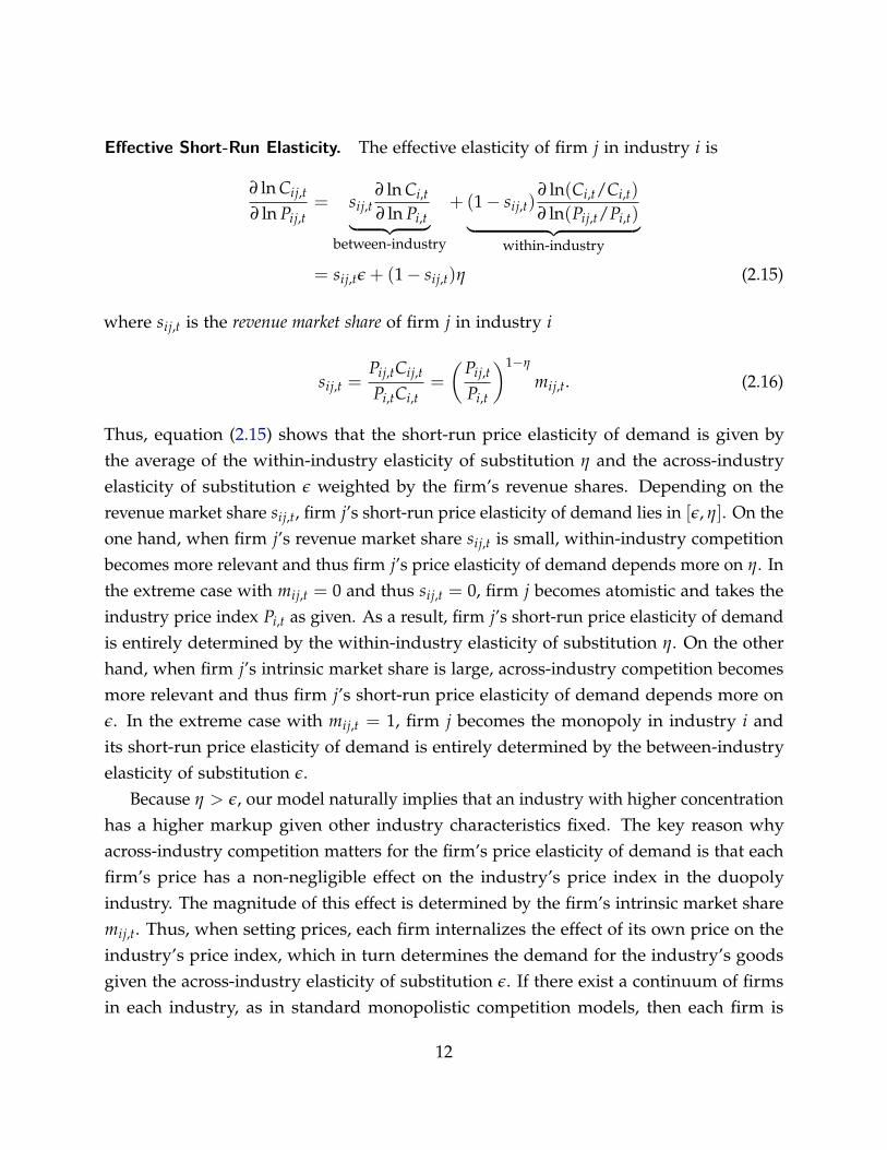
Effective Short-Run Elasticity. The effective elasticity of firm j in industry i is

∂ ln Cij,t

∂ ln Pij,t= sij,t

∂ ln Ci,t

∂ ln Pi,t︸ ︷︷ ︸between-industry

+ (1− sij,t)∂ ln(Ci,t/Ci,t)

∂ ln(Pij,t/Pi,t)︸ ︷︷ ︸within-industry

= sij,tε + (1− sij,t)η (2.15)

where sij,t is the revenue market share of firm j in industry i

sij,t =Pij,tCij,t

Pi,tCi,t=

(Pij,t

Pi,t

)1−η

mij,t. (2.16)

Thus, equation (2.15) shows that the short-run price elasticity of demand is given bythe average of the within-industry elasticity of substitution η and the across-industryelasticity of substitution ε weighted by the firm’s revenue shares. Depending on therevenue market share sij,t, firm j’s short-run price elasticity of demand lies in [ε, η]. On theone hand, when firm j’s revenue market share sij,t is small, within-industry competitionbecomes more relevant and thus firm j’s price elasticity of demand depends more on η. Inthe extreme case with mij,t = 0 and thus sij,t = 0, firm j becomes atomistic and takes theindustry price index Pi,t as given. As a result, firm j’s short-run price elasticity of demandis entirely determined by the within-industry elasticity of substitution η. On the otherhand, when firm j’s intrinsic market share is large, across-industry competition becomesmore relevant and thus firm j’s short-run price elasticity of demand depends more onε. In the extreme case with mij,t = 1, firm j becomes the monopoly in industry i andits short-run price elasticity of demand is entirely determined by the between-industryelasticity of substitution ε.

Because η > ε, our model naturally implies that an industry with higher concentrationhas a higher markup given other industry characteristics fixed. The key reason whyacross-industry competition matters for the firm’s price elasticity of demand is that eachfirm’s price has a non-negligible effect on the industry’s price index in the duopolyindustry. The magnitude of this effect is determined by the firm’s intrinsic market sharemij,t. Thus, when setting prices, each firm internalizes the effect of its own price on theindustry’s price index, which in turn determines the demand for the industry’s goodsgiven the across-industry elasticity of substitution ε. If there exist a continuum of firmsin each industry, as in standard monopolistic competition models, then each firm is

12

atomic and has no influence on the industry’s price index. As a result, across-industrycompetition would have no impact on firms’ price elasticities of demand.

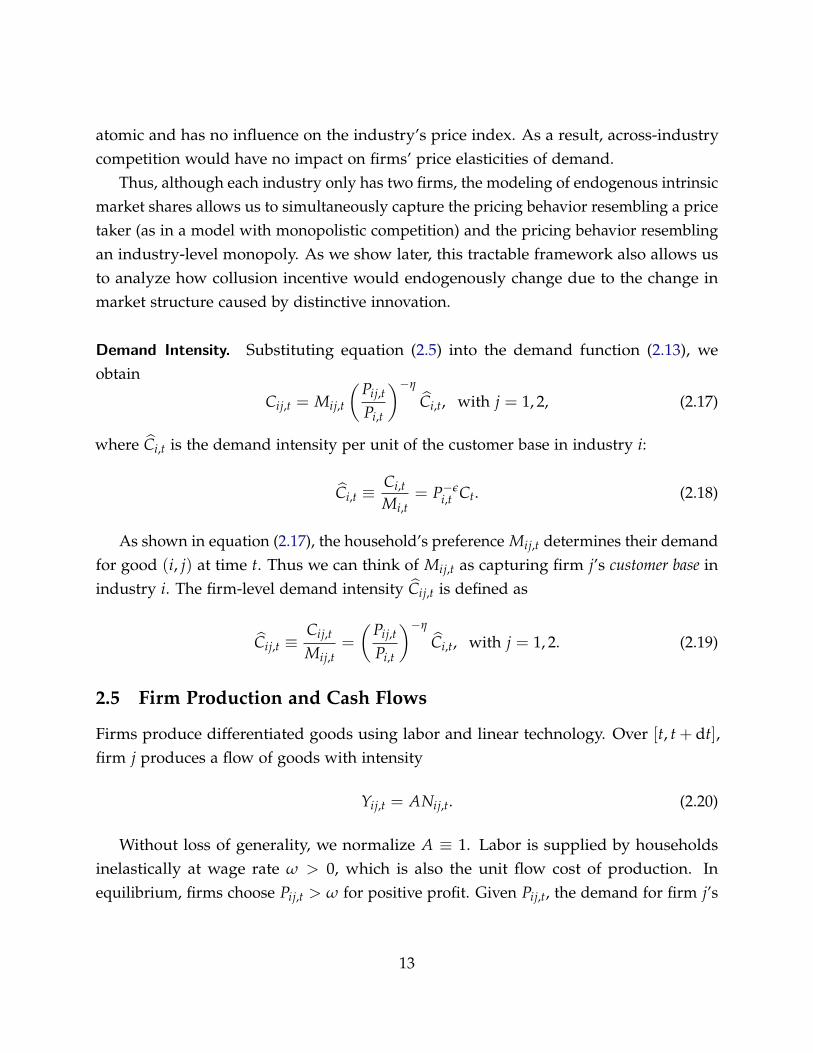
Thus, although each industry only has two firms, the modeling of endogenous intrinsicmarket shares allows us to simultaneously capture the pricing behavior resembling a pricetaker (as in a model with monopolistic competition) and the pricing behavior resemblingan industry-level monopoly. As we show later, this tractable framework also allows usto analyze how collusion incentive would endogenously change due to the change inmarket structure caused by distinctive innovation.

Demand Intensity. Substituting equation (2.5) into the demand function (2.13), weobtain

Cij,t = Mij,t

(Pij,t

Pi,t

)−η

Ci,t, with j = 1, 2, (2.17)

where Ci,t is the demand intensity per unit of the customer base in industry i:

Ci,t ≡Ci,t

Mi,t= P−ε

i,t Ct. (2.18)

As shown in equation (2.17), the household’s preference Mij,t determines their demandfor good (i, j) at time t. Thus we can think of Mij,t as capturing firm j’s customer base inindustry i. The firm-level demand intensity Cij,t is defined as

Cij,t ≡Cij,t

Mij,t=

(Pij,t

Pi,t

)−η

Ci,t, with j = 1, 2. (2.19)

2.5 Firm Production and Cash Flows

Firms produce differentiated goods using labor and linear technology. Over [t, t + dt],firm j produces a flow of goods with intensity

Yij,t = ANij,t. (2.20)

Without loss of generality, we normalize A ≡ 1. Labor is supplied by householdsinelastically at wage rate ω > 0, which is also the unit flow cost of production. Inequilibrium, firms choose Pij,t > ω for positive profit. Given Pij,t, the demand for firm j’s

13

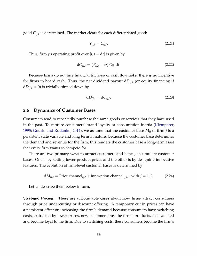
good Cij,t is determined. The market clears for each differentiated good:

Yij,t = Cij,t. (2.21)

Thus, firm j’s operating profit over [t, t + dt] is given by

dOij,t =(

Pij,t −ω)

Cij,tdt. (2.22)

Because firms do not face financial frictions or cash flow risks, there is no incentivefor firms to hoard cash. Thus, the net dividend payout dDij,t (or equity financing ifdDij,t < 0) is trivially pinned down by

dDij,t = dOij,t. (2.23)

2.6 Dynamics of Customer Bases

Consumers tend to repeatedly purchase the same goods or services that they have usedin the past. To capture consumers’ brand loyalty or consumption inertia (Klemperer,1995; Gourio and Rudanko, 2014), we assume that the customer base Mij of firm j is apersistent state variable and long term in nature. Because the customer base determinesthe demand and revenue for the firm, this renders the customer base a long-term assetthat every firm wants to compete for.

There are two primary ways to attract customers and hence, accumulate customerbases. One is by setting lower product prices and the other is by designing innovativefeatures. The evolution of firm-level customer bases is determined by

dMij,t = Price channelij,t + Innovation channelij,t, with j = 1, 2. (2.24)

Let us describe them below in turn.

Strategic Pricing. There are uncountable cases about how firms attract consumersthrough price undercutting or discount offering. A temporary cut in prices can havea persistent effect on increasing the firm’s demand because consumers have switchingcosts. Attracted by lower prices, new customers buy the firm’s products, feel satisfiedand become loyal to the firm. Due to switching costs, these consumers become the firm’s

14

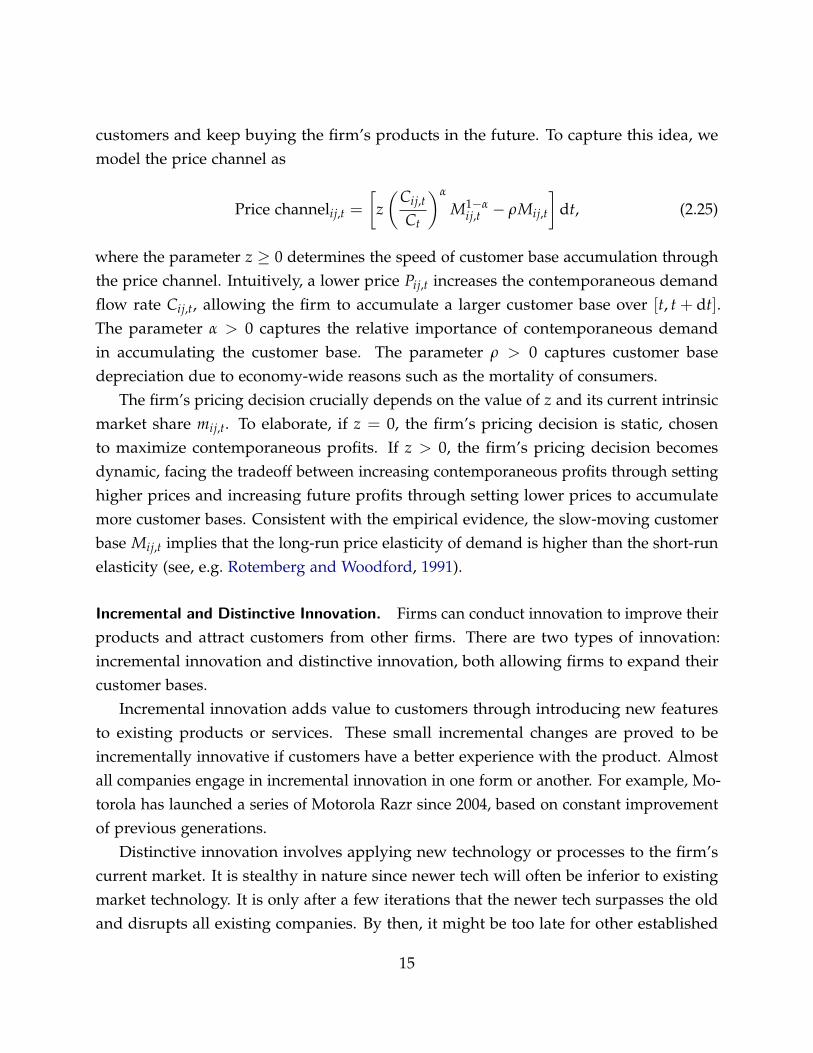
customers and keep buying the firm’s products in the future. To capture this idea, wemodel the price channel as

Price channelij,t =[

z(

Cij,t

Ct

)α

M1−αij,t − ρMij,t

]dt, (2.25)

where the parameter z ≥ 0 determines the speed of customer base accumulation throughthe price channel. Intuitively, a lower price Pij,t increases the contemporaneous demandflow rate Cij,t, allowing the firm to accumulate a larger customer base over [t, t + dt].The parameter α > 0 captures the relative importance of contemporaneous demandin accumulating the customer base. The parameter ρ > 0 captures customer basedepreciation due to economy-wide reasons such as the mortality of consumers.

The firm’s pricing decision crucially depends on the value of z and its current intrinsicmarket share mij,t. To elaborate, if z = 0, the firm’s pricing decision is static, chosento maximize contemporaneous profits. If z > 0, the firm’s pricing decision becomesdynamic, facing the tradeoff between increasing contemporaneous profits through settinghigher prices and increasing future profits through setting lower prices to accumulatemore customer bases. Consistent with the empirical evidence, the slow-moving customerbase Mij,t implies that the long-run price elasticity of demand is higher than the short-runelasticity (see, e.g. Rotemberg and Woodford, 1991).

Incremental and Distinctive Innovation. Firms can conduct innovation to improve theirproducts and attract customers from other firms. There are two types of innovation:incremental innovation and distinctive innovation, both allowing firms to expand theircustomer bases.

Incremental innovation adds value to customers through introducing new featuresto existing products or services. These small incremental changes are proved to beincrementally innovative if customers have a better experience with the product. Almostall companies engage in incremental innovation in one form or another. For example, Mo-torola has launched a series of Motorola Razr since 2004, based on constant improvementof previous generations.

Distinctive innovation involves applying new technology or processes to the firm’scurrent market. It is stealthy in nature since newer tech will often be inferior to existingmarket technology. It is only after a few iterations that the newer tech surpasses the oldand disrupts all existing companies. By then, it might be too late for other established

15

firms to quickly compete with the newer technology. There are quite a few examples ofdistinctive innovation, one of the more prominent being Apple’s iPhone disruption of themobile phone market.7

In our model, we assume that each firm’s incremental innovation and distinctiveinnovation succeed independently with different intensities φi,tλι and (1− φi,t)λd. Theindustry characteristic φi,t reflects the units of incremental R&D projects that firmshave in industry i, and 1 − φi,t reflects the units of distinctive R&D projects, or theindustry’s capacity of distinctive innovation. φi,t is the only ex-ante heterogeneity acrossindustries, evolving idiosyncratically according to a finite-state Markov chain on Φ =

{0 ≤ φ1 < φ2 < ... < φN ≤ 1}.Conditional on successful innovations, incremental and distinctive innovations sepa-

rately create new customer bases with rate gι and gd. In addition, successful innovationalso snatches the peer firm’s customer bases by τι and τd fractions. We emphasize thedifference in the customer base competition effect between the two types of innovation byassuming

0 ≈ τι << τd ≈ 1 and λι >> λd ≥ 0, (2.26)

so that distinctive innovation happens rarely but allows firms to capture almost the entireindustry’s market share. The average growth effects from the two types of innovation areassumed to be equal, i.e. λιgι = λdgd.

Thus, the innovation channel for customer base accumulation is given by

Innovation channelij,t =[τιdI ι

ij,t + τddIdij,t

]Mik,t︸ ︷︷ ︸

j’s competition effect

+[

gιdI ιij,t + gddId

ij,t

]Mi,t︸ ︷︷ ︸

j’s growth effect

−[τιdI ι

ik,t + τddIdik,t

]Mij,t,︸ ︷︷ ︸

k’s competition effect

(2.27)

where I ιij,t and Id

ij,t are independent Poisson processes with intensity φi,tλι and (1− φi,t)λd,capturing the success of incremental and distinctive innovation.

7Prior to the iPhone, most popular phones relied on buttons, keypads or scroll wheels for user input.The iPhone was the result of a technological movement that was years in making, mostly iterated by PalmTreo phones and personal digital assistants (PDAs). In order to disrupt the mobile phone market, Applecobbled together an amazing touch screen that had a simple to use interface, and provided users access toa large assortment of built-in and third-party mobile applications.

16

Evolution of Customer Bases. Substituting the price channel (2.25) and the innovationchannel (2.27) into equation (2.24), we derive the evolution of firm j’s customer base

dMij,t =

[z(

Cij,t

Ct

)α

M1−αij,t − ρMij,t

]dt +

(τιdI ι

ij,t + τddIdij,t

)Mik,t

+(

gιdI ιij,t + gddId

ij,t

)Mi,t −

(τιdI ι

ik,t + τddIdik,t

)Mij,t. (2.28)

The evolution of industry i’s aggregate customer base is

dMi,t

Mi,t=

[z

(∑j∈F

mij,tCαij,t

)− ρ

]dt + ∑

j∈F

(gιdI ι

ij,t + gddIdij,t

). (2.29)

Therefore, the growth rate of each industry i’s customer base is the average growthrate of the two firms’ customer bases weighted by their intrinsic market shares:

dMi,t

Mi,t= ∑

j∈Fmij,t

dMij,t

Mij,t. (2.30)

2.7 Price Setting Supergames

In this section, we illustrate the rich interactions among firms in the same industry.Essentially, the two firms in the same industry play a stochastic dynamic game. As timeis continuous, the stage game of setting prices are played continuously and infinitelyrepeated. In this setting, there exist multiple equilibria because one can apply a conditionalpunishment strategy to sustain some specific payoff distribution. Below, we first illustratethe non-collusive equilibrium. Then we define and characterize the collusive equilibriumthat yields higher profits for both firms.

Non-Collusive Equilibrium. Substituting equation (2.17) into equation (2.23), we obtain

dDij,t

Mij,t= Πij(Pi1,t, Pi2,t, Mi1,t, Mi2,t, Ct)dt, (2.31)

17

where Πij(Pi1,t, Pi2,t, Mi1,t, Mi2,t, Ct) is the conditional expected profit rate defined by8

Πij(Pi1,t, Pi2,t, Mi1,t, Mi2,t, Ct) ≡(

Pij,t −ω) (Pij,t

Pi,t

)−η

P−εi,t Ct. (2.32)

Equation (2.32) shows that the (local) conditional expected profit rate of firm j dependson its peer firm k’s product price Pik,t through the industry’s price index Pi,t. This reflectsthe externality of firm k’s decisions. For example, if firm k sets a low price Pik,t, the priceindex Pi,t will drop, and thus the demand for firm j’s goods Cij,t will decrease. This willmotivate firm j to set a lower price Pij,t, and thus the two firms’ pricing decisions exhibitstrategic complementarity in equilibrium.

In the non-collusive equilibrium, firm j chooses product price Pij,t to maximize share-holder value VN

ij (Mi1,t, Mi2,t, φi,t, Ct, θt), conditional on its peer firm k setting the equilib-rium price PN

ik,t. The firm’s value also depends on persistent consumption growth rate θt

because it affects the state-price density Λt. Following the standard recursive formulationin dynamic games with Markov Perfect Nash Equilibrium (see, e.g. Pakes and McGuire,1994; Ericson and Pakes, 1995; Maskin and Tirole, 2001), the optimization problem forfirm 1 can be formulated recursively by an HJB equation:

0 = maxPi1,t

ΛtΠi1(Pi1,t, PNi2,t, Mi1,t, Mi2,t, Ct)Mij,tdt + Et

[d(ΛtVN

i1 (Mi1,t, Mi2,t, φi,t, Ct, θt))]

.

(2.33)Similarly, the optimization problem for firm 2 is given by the following HJB equation:

0 = maxPi2,t

ΛtΠi2(PNi1,t, Pi2,t, Mi1,t, Mi2,t, Ct)Mij,tdt + Et

[d(ΛtVN

i2 (Mi1,t, Mi2,t, φi,t, Ct, θt))]

(2.34)The non-collusive equilibrium prices PN

ij,t(Mi1,t, Mi2,t, φi,t, Ct, θt) (with j = 1, 2) aredetermined by solving the coupled HJB equations (2.33-2.34).

A couple of points are worth mentioning. First, the expectation Et is conditioning onthe exogenous state variable φi,t, Ct, θt and endogenous state variables Mi1,t and Mi2,t.Second, The expectation is also conditioning on the endogenous control variables, Pij,t andPik,t, because they determine the evolution of endogenous state variables (see equation2.28). Third, the Nash equilibrium considered here is non-collusive, because it does

8Note we define the conditional expected profit rate as Πij(Pi1,t, Pi2,t, Mi1,t, Mi2,t, Ct) rather thanΠij(Pij,t, Pik,t, Mij,t, Mik,t, Ct) because we want to keep the order of state variables the same when weconsider j = 1 (k = 2) and j = 2 (k = 1).

18

not depend on historical information (i.e. not using conditional punishment strategiesbased on the two firms’ historical decisions). Such an equilibrium is called “static Nashequilibrium” by Fudenberg and Tirole (1991). Fourth, the non-collusive equilibriumis actually the equilibrium of a dynamic game because the strategic pricing decisionsinvolve dynamic concerns. Each firm j’s price Pij,t not only affects both firms’ contempo-raneous cash flows through the current price index Pi,t but also their continuation valuesdVN

ij (Mi1,t, Mi2,t, φi,t, Ct, θt) due to the price channel specified in equation (2.25).

Collusive Equilibrium. The non-collusive equilibrium features low product prices andlow operating profits due to the lack of collusion. In a dynamic setting, the repeatedinteractions between the two firms within the same industry naturally motivate theformation of a cartel, in which firms collectively set higher prices to gain higher operatingprofits. We define the collusive equilibrium as the sub-game perfect equilibrium in whichthe two firms adopt prices higher than non-collusive prices.9

Consider a collusive equilibrium in which firms follow the collusive pricing schedulePC

ij (Mi1,t, Mi2,t, φi,t, Ct, θt) (with j = 1, 2).10 Firm j’s value in the collusive equilibrium,denoted by VC

ij (Mi1,t, Mi2,t, φi,t, Ct, θt), is determined by

0 = ΛtΠij(PCi1, PC

i2, Mi1,t, Mi2,t, Ct)Mij,tdt+Et

[d(ΛtVC

ij (Mi1,t, Mi2,t, φi,t, Ct, θt))]

, with j = 1, 2.(2.35)

The sub-game perfection of the collusive equilibrium is ensured by conditional strate-gies with punishment on deviation. In particular, we assume that firms receive theopportunity to inspect peers’ past prices up to t with Poisson intensity ς over [t, t + dt].11

When a price deviation is detected by the peer firm, the peer firm will start setting thenon-collusive price in the future. Conditional on the peer firm’s price being non-collusive,

9In the industrial organization and macroeconomics literature, this equilibrium is called collusiveequilibrium or collusion (see e.g. Green and Porter, 1984; Rotemberg and Saloner, 1986). Game theoristsgenerally call it the equilibrium of repeated game (Fudenberg and Tirole, 1991) in order to distinguish itsnature from the equilibrium of stage games (i.e. our non-collusive equilibrium).

10Fershtman and Pakes (2000) require all firms to adopt the same collusive price to maintain tractability.Our collusive pricing schedule is more general because it allows firms to set different prices based on theircustomer bases, the industry’s characteristic, and aggregate conditions.

11In discrete time, a standard assumption in dynamic game-theoretic models is that deviation is observedin the next period. This assumption, however, is unrealistic in a continuous time model. If we assumethat deviation is observed in the next instant, it means that information flows infinitely fast, then anyaverage payoffs can be achieved by a sub-game perfect equilibrium. Bergin and MacLeod (1993) discuss thetechnical difficulties in continuous-time repeated games.

19

the deviating firm would also set the non-collusive price after her deviation is detected,because setting the non-collusive price is the best response to the peer firm’s non-collusiveprice. Thus, the punishment on deviation is based on switching to the non-collusiveequilibrium, which itself has sub-game perfection.12 The collusive equilibrium is a sub-game perfect equilibrium if the collusive pricing schedule PC

ij (Mi1,t, Mi2,t, φi,t, Ct, θt) isset to ensure that there is no deviation along the equilibrium path. Formally, denoteVD

ij (Mi1,t, Mi2,t, φi,t, Ct, θt) as firm j’s value conditional on one-shot deviation13, the HJBequations are:

0 =maxPi1,t

ΛtΠi1(Pi1, PCi2, Mi1,t, Mi2,t, Ct)Mi1,tdt + Et

[d(ΛtVD

i1 (Mi1,t, Mi2,t, φi,t, Ct, θt))]

+ Λt

[VN

i1 (Mi1,t, Mi2,t, φi,t, Ct, θt)−VDi1 (Mi1,t, Mi2,t, φi,t, Ct, θt)

]ςdt, (2.36)

0 =maxPi2,t

ΛtΠi2(PCi1, Pi2, Mi1,t, Mi2,t, Ct)Mi2,tdt + Et

[d(ΛtVD

i2 (Mi1,t, Mi2,t, φi,t, Ct, θt))]

+ Λt

[VN

i2 (Mi1,t, Mi2,t, φi,t, Ct, θt)−VDi2 (Mi1,t, Mi2,t, φi,t, Ct, θt)

]ςdt. (2.37)

To ensure that the collusive equilibrium with the pricing schedule PCij (Mi1,t, Mi2,t, φi,t, Ct, θt)

is a sub-game perfect equilibrium, there must be no deviation along the equilibrium path.Thus the following incentive compatibility (IC) constraints have to be satisfied:

VDij (Mi1,t, Mi2,t, φi,t, Ct, θt) ≤ VC

ij (Mi1,t, Mi2,t, φi,t, Ct, θt), (2.38)

for j = 1, 2, Mi1,t, Mi2,t > 0, φi,t ∈ Φ, Ct > 0, and all θt. In fact, there exist infinitely manycollusive pricing schedules PC

ij (Mi1,t, Mi2,t, φi,t, Ct, θt) that satisfy the IC constraints, andhence infinitely many collusive equilibrium. Because firms maximize profits in generalequilibrium, it is reasonable for them two collude on prices as high as possible.14 We

12We adopt the non-collusive equilibrium as the incentive-compatible punishment for deviation tofollow the literature (see, e.g. Green and Porter, 1984; Rotemberg and Saloner, 1986). The non-collusiveequilibrium can be interpreted as the most severe price war, though it never happens in equilibrium. Allelse equal, adopting a less stringent punishment would lower collusive prices. In a similar multi-periodgame, Bond and Krishnamurthy (2004) consider a lenient “debt-default” rule as a punishment for debtdefault, rather than a full exclusion from financial markets. Interestingly, the “debt-default” rule providesoptimal repayment incentives while at the same time resembles laws governing default on debt contracts.

13The one-shot deviation principle indicates that there is no need to consider the case with two firmssimultaneously deviating from collusive pricing to obtain a sub-game perfect equilibrium (see Fudenbergand Tirole, 1991).

14There are two reasons why we focus on the highest collusive pricing schedule. First, non-binding ICconstraints imply that there is room to further increase both firms’ values by increasing collusive prices.

20

thus focus on the highest collusive pricing schedule, under which the IC constraints arebinding, i.e. PC

ij (Mi1,t, Mi2,t, φi,t, Ct, θt) are determined such that

VDij (Mi1,t, Mi2,t, φi,t, Ct, θt) = VC

ij (Mi1,t, Mi2,t, φi,t, Ct, θt). (2.39)

Intuitively, a higher ς increases the likelihood of implementing the punishment strategy,dampening the incentive to deviate by reducing VD

ij (Mi1,t, Mi2,t, φi,t, Ct, θt). Thus, all elseequal, a higher ς allows firms to collude on higher prices. Importantly, the collusionincentive also depends on the long-run growth rate θt and its persistence.15 We discussthem in Section 4.

2.8 General Equilibrium Conditions

In equilibrium, the value function of the representative household is

Ut = exp (A0 + A1θt)W1−γ

t1− γ

, (2.40)

where A0 is a deterministic function of model parameters, and A1 is equal to

A1 =ψ−1(1− γ)

h + κ, with h = exp

(ln C− ln W

). (2.41)

The equilibrium wealth-consumption ratio is

Wt

Ct= ρ−ψ exp

[1− ψ

1− γA0 +

(1− ψ−1

h + κ

)θt

]. (2.42)

In equilibrium, the long-run deterministic steady-state consumption-wealth ratio is:

ln(h) = ln C− ln W = ψ ln(ρ)− 1− ψ

1− γA0 −

1− ψ−1

h + κθ. (2.43)

Given that firms collude with each other to maximize their values, it is a bit unreasonable to rule out abetter collusion. Second, considering the highest collusive price allows us to conduct more disciplinedcomparative statics in the presence of multiple equilibria. In other words, focusing on the highest collusiveprice ensures that we always pick up the same equilibrium when we compare across different industries.

15We do not model dynamic entries and exits due to the complexity of the current setup. Introducingentries and exits will strengthen our mechanism by increasing the magnitude of price war risks. Intuitively,it becomes even harder for firms to collude during periods with low long-run growth rates because exitsare more likely due to lower operating cash flows.

21

2.9 Model Solution

By exploiting linearity on Mi,tCt, we reduce the model to three state variables: mi1,t,φi,t, and θt. We solve the normalized firm value vN

ij (mi1,t, φi,t, θt), vCij(mi1,t, φi,t, θt), and

vDij (mi1,t, φi,t, θt). The details of our numerical algorithm are presented in Appendix D.

We solve the model in risk-neutral measure. By Girsanov’s theorem, we have

dZc,t =− λcdt + dZc,t, (2.44)

dZθ,t =− λθdt + dZθ,t. (2.45)

Under the risk-neutral measure, the dynamics of aggregate conditions are

dCt

Ct=θtdt + σcdZc,t, (2.46)

dθt =κ(

θQ − θt

)dt + ϕθσcdZθ,t, (2.47)

whereθ

Q= θ − λcσc − κ−1λθ ϕθσc. (2.48)

3 Illustration of Equilibrium Concepts

Our model is based on a general equilibrium framework with a continuum of industries.Within each industry, we formulate the two firms’ dynamic competition using stochasticgame-theoretic models. In this section, we illustrate the dynamic game-theoretic equilib-rium within an industry. We start by illustrating the non-collusive equilibrium in Section3.1. We highlight that the strategic complementarity embedded in the non-collusiveequilibrium is a crucial force that generates price wars during periods with low long-runconsumption growth. We then illustrate the collusive equilibrium that naturally arisesfrom the dynamic repeated interaction between the two firms. The collusive equilib-rium is a sub-game perfect equilibrium that is endogenously sustained by using thenon-collusive equilibrium as punishment. In Section 3.3, we illustrate the IC constraintsand the determination of collusive prices in the collusive equilibrium.

22

3.1 Non-Collusive Equilibrium

In the non-collusive equilibrium, the two firms simultaneously set prices, taking the otherfirm’s price as given. Thus, the equilibrium prices are determined by the intersection ofthe two firms’ optimal price as a function of the other firm’s price. To characterize thedetermination of the non-collusive equilibrium, we consider an industry with φ = 0 andlong-run growth rate θ = 0.06. Denote PN

i1 (mi1; Pi2) as firm 1’s optimal price as a functionof its intrinsic market share mi1 and firm 2’s price Pi2. Similarly, we denote PN

i2 (mi1; Pi1)

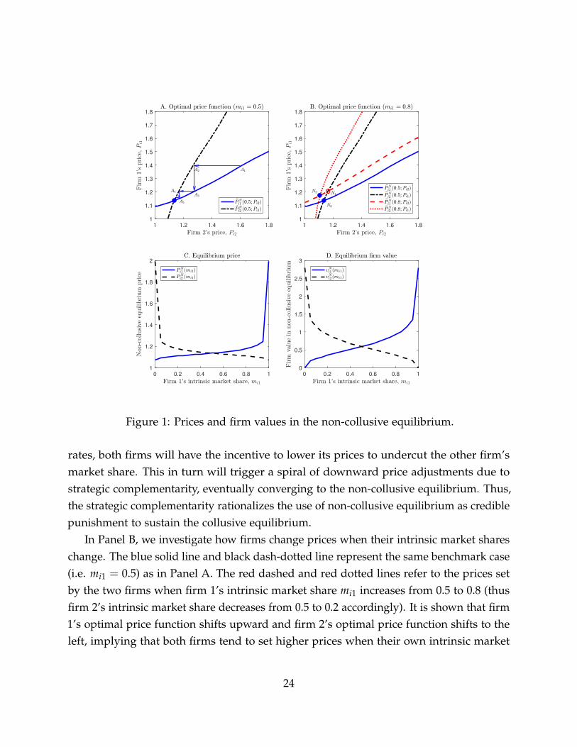
as firm 2’s optimal price as a function of firm 1’s intrinsic market share mi1 and price Pi1.In Panel A of Figure 1, the blue solid line plots firm 1’s optimal price as a function of

firm 2’s price Pi2, when the two firms have equal intrinsic market shares (i.e. mi1 = 0.5).The black dash-dotted line plots firm 2’s optimal price as a function of firm 1’s price Pi1

for the same intrinsic market share. The intersection of the two curves (the blue filledcircle) determines the equilibrium prices, i.e. PN

i1 (0.5) and PNi2 (0.5):

PNi1 (0.5) = PN

i1 (0.5; PNi2 (0.5)) and PN

i2 (0.5) = PNi2 (0.5; PN

i1 (0.5)). (3.1)

The two firms set exactly the same prices when they have the same intrinsic marketshares. Both curves are upward sloping, indicating that there exists strategic comple-mentarity in setting prices in the non-collusive equilibrium: both firms tend to set lowerprices when the other firm’s price is lower. This is because when the other firm’s price islower, the price elasticity of demand endogenously increases, motivating the firm to lowerits own price. Because of such strategic complementarity, the non-collusive equilibriumfeatures low prices and hence low profit margins for both firms. To see it clearly, supposefirm 2 sets Pi2 = 1.6, then firm 1’s best response is to set Pi1 = 1.4 (A1). Given that firm 1’sprice is lower than firm 2’s, firm 2 will further lower its price to Pi2 = 1.28 (A2). But thenfirm 2’s price is lower than firm 1’s, which triggers firm 1 to lower its price to Pi1 = 1.2(A3), and so on, until the prices reach equilibrium values. Such price adjustments happeninstantaneously in rational expectation equilibrium.16

We emphasize that the strategic complementarity in price setting is a crucial force thatgenerates price wars from declines in long-run consumption growth. As we discuss inSection 4.1, collusive prices decrease with long-run growth rates in consumption. This isbecause if firms were to collude on high prices during periods with low long-run growth

16The dynamics of price adjustment is related to the old tradition that used Tatonnement or Cobwebdynamics to capture the off-equilibrium adjustment of prices in Walrasian economies.

23

1 1.2 1.4 1.6 1.8

1

1.1

1.2

1.3

1.4

1.5

1.6

1.7

1.8

1 1.2 1.4 1.6 1.8

1

1.1

1.2

1.3

1.4

1.5

1.6

1.7

1.8

0 0.2 0.4 0.6 0.8 1

1

1.2

1.4

1.6

1.8

2

0 0.2 0.4 0.6 0.8 1

0

0.5

1

1.5

2

2.5

3

Figure 1: Prices and firm values in the non-collusive equilibrium.

rates, both firms will have the incentive to lower its prices to undercut the other firm’smarket share. This in turn will trigger a spiral of downward price adjustments due tostrategic complementarity, eventually converging to the non-collusive equilibrium. Thus,the strategic complementarity rationalizes the use of non-collusive equilibrium as crediblepunishment to sustain the collusive equilibrium.

In Panel B, we investigate how firms change prices when their intrinsic market shareschange. The blue solid line and black dash-dotted line represent the same benchmark case(i.e. mi1 = 0.5) as in Panel A. The red dashed and red dotted lines refer to the prices setby the two firms when firm 1’s intrinsic market share mi1 increases from 0.5 to 0.8 (thusfirm 2’s intrinsic market share decreases from 0.5 to 0.2 accordingly). It is shown that firm1’s optimal price function shifts upward and firm 2’s optimal price function shifts to theleft, implying that both firms tend to set higher prices when their own intrinsic market

24

shares increase. Intuitively, there are two main reasons. First, when the intrinsic marketshare is higher, setting low prices to further compete for the market share is relativelymore costly compared to setting high prices to profit from inertial customers. Second, thefirm’s influence on the equilibrium price index increases with its intrinsic market share(see equation 2.14). Therefore, a higher market share increases the firm’s market powerand lowers the price elasticity of demand, resulting in higher prices.

Panel B also clearly illustrates the implication of strategic pricing. In the benchmarkequilibrium (N0), the prices are Pi1,N0 and Pi2,N0 . A higher market share mi1 shifts theequilibrium to N2, and the new equilibrium prices satisfy Pi1,N2 > Pi1,N0 and Pi2,N2 < Pi2,N0 .However, if firm 2 were to hold its price decisions unchanged (at the black-dashed line),the new equilibrium would be N1, with Pi1,N1 > Pi1,N2 , indicating that firm 1 would raiseits price more in response to the increase in its intrinsic market share mi1. Therefore, firm1’s price is less responsive precisely because it anticipates that firm 2 would lower itsprice Pi2 (as captured by the red dotted line). Such strategic concerns result in a smallerincrease in firm 1’s price Pi1, which helps prevent too much loss in its intrinsic marketshare mi1.

Panel C shows that when firm 1’s intrinsic market share increases, firm 1’s valueincreases (the blue solid line) and firm 2’s value decreases symmetrically (black dashedline). Moreover, both firms set higher equilibrium prices when their intrinsic marketshares increase (see Panel D).

3.2 Collusive Equilibrium

We now turn to the illustration of the collusive equilibrium. In the collusive equilibrium,both firms set prices according to the collusive pricing schedule Pij(mi1,t, φi,t, θt). Weillustrate the collusive equilibrium with φ = 0 and θ = 0.06 below.

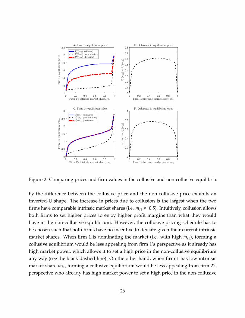
In Panel A of Figure 2, we compare the firm’s prices in the collusive equilibriumand the non-collusive equilibrium. As the two firms are symmetric, we only focus onillustrating firm 1’s price. The black dashed line plots firm 1’s price in the non-collusiveequilibrium (as in Panel C of Figure 1). The blue solid line plots firm 1’s price in thecollusive equilibrium. It is shown that due to collusion, firm 1 sets higher prices thanwhat it would set in the non-collusive equilibrium. The prices increase monotonicallywith intrinsic market shares in both the collusive and the non-collusive equilibria.

Interestingly, Panel B shows that the ability to collude on higher prices, as reflected

25

0 0.2 0.4 0.6 0.8 1

1

1.2

1.4

1.6

1.8

2

2.2

0 0.2 0.4 0.6 0.8 1

0

0.1

0.2

0.3

0.4

0.5

0.6

0.7

0.8

0 0.2 0.4 0.6 0.8 1

0

0.5

1

1.5

2

2.5

3

0 0.2 0.4 0.6 0.8 1

0

0.2

0.4

0.6

0.8

1

Figure 2: Comparing prices and firm values in the collusive and non-collusive equilibria.

by the difference between the collusive price and the non-collusive price exhibits aninverted-U shape. The increase in prices due to collusion is the largest when the twofirms have comparable intrinsic market shares (i.e. mi1 ≈ 0.5). Intuitively, collusion allowsboth firms to set higher prices to enjoy higher profit margins than what they wouldhave in the non-collusive equilibrium. However, the collusive pricing schedule has tobe chosen such that both firms have no incentive to deviate given their current intrinsicmarket shares. When firm 1 is dominating the market (i.e. with high mi1), forming acollusive equilibrium would be less appealing from firm 1’s perspective as it already hashigh market power, which allows it to set a high price in the non-collusive equilibriumany way (see the black dashed line). On the other hand, when firm 1 has low intrinsicmarket share mi1, forming a collusive equilibrium would be less appealing from firm 2’sperspective who already has high market power to set a high price in the non-collusive

26

equilibrium. Thus, it is easier to collude on relatively higher prices when firm 1 and firm2 have comparable intrinsic market shares.

The above intuition is more clearly seen in two extreme cases. When firm 1’s intrinsicmarket share mi1 ≈ 1, Panel A shows that it sets a price close to ε

ε−1 ω = 2. This is theprice that firm 1 would choose facing a price elasticity of demand ε. In this case, firm1 essentially acts almost as a monopoly in industry i and sets prices to compete withfirms in other industries. Thus, the constant across-industry price elasticity of demandis what determines firm 1’s optimal price in both the collusive and the non-collusiveequilibria. By contrast, when firm 1’s intrinsic market share mi1 ≈ 0, Panel A shows thatit sets a price close to η

η−1 ω = 1.07. This is the price that firm 1 would choose facing aprice elasticity of demand η. In this case, firm 1 essentially acts almost as a price takerin industry i because it has little market power to influence the industry’s price index.Thus, the constant within-industry price elasticity of demand is what determines firm 1’soptimal price in both the collusive and the non-collusive equilibria.

Panel C compares firm 1’s value in the collusive and the non-collusive equilibria.Colluding on higher prices increases firm 1’s profit margins, leading to higher firm values.Not surprisingly, due to the inverted-U collusive prices, the difference in firm valuesdisplays a similar inverted-U shape (Panel D) when the intrinsic market share varies.

3.3 Determination of Collusive Prices

In this section, we clarify how the collusive prices are determined in equilibrium. In PanelA of Figure 2, the red line plots the optimal price that firm 1 would choose conditionalon its deviation from the collusive pricing schedule.17 It shows that the optimal deviationprice is always lower than the collusive price. This is intuitive because firms colludeon higher prices relative to what they would set in the non-collusive equilibrium, andthus both firms have the incentive to undercut the other firms in order to increase bothcontemporaneous demand and gain more intrinsic market shares. Whether firm 1 woulddeviate depends on what deviation value firm 1 would obtain by setting the optimaldeviation price. Intuitively, there are countervailing forces that determine the gains from

17Here, we follow the standard game theory by considering one-shot deviation. That is, we considerwhat the deviation price that firm 1 would choose conditional on firm 2 not deviating from the collusiveequilibrium. The one-shot deviation property ensures that no profitable one-shot deviations for everyplayer is a necessary and sufficient condition for a strategy profile of a finite extensive-form game to form asub-game perfect equilibrium.

27

deviation. If deviation is not detected by firm 2, then firm 1 would gain by stealingintrinsic market shares from firm 2 through lower prices. However, if deviation is detectedby firm 2, then firm 1 will be punished by switching to the non-collusive equilibriumwhich features low prices and low profit margins.

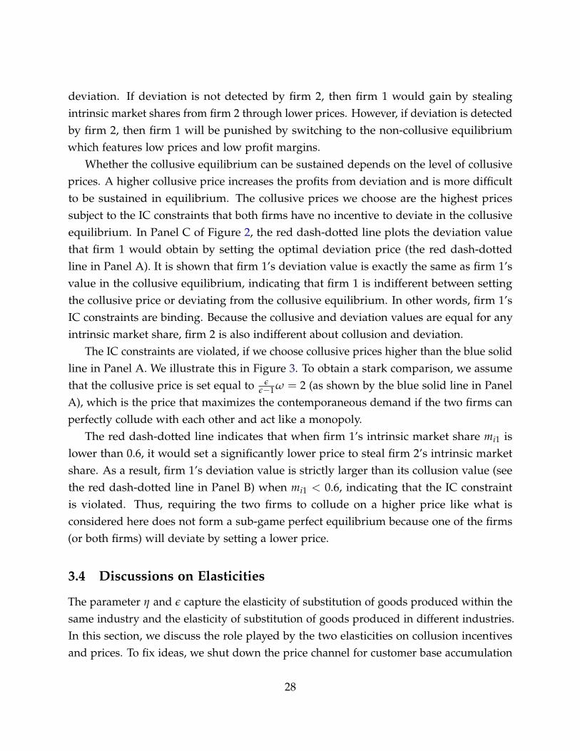
Whether the collusive equilibrium can be sustained depends on the level of collusiveprices. A higher collusive price increases the profits from deviation and is more difficultto be sustained in equilibrium. The collusive prices we choose are the highest pricessubject to the IC constraints that both firms have no incentive to deviate in the collusiveequilibrium. In Panel C of Figure 2, the red dash-dotted line plots the deviation valuethat firm 1 would obtain by setting the optimal deviation price (the red dash-dottedline in Panel A). It is shown that firm 1’s deviation value is exactly the same as firm 1’svalue in the collusive equilibrium, indicating that firm 1 is indifferent between settingthe collusive price or deviating from the collusive equilibrium. In other words, firm 1’sIC constraints are binding. Because the collusive and deviation values are equal for anyintrinsic market share, firm 2 is also indifferent about collusion and deviation.

The IC constraints are violated, if we choose collusive prices higher than the blue solidline in Panel A. We illustrate this in Figure 3. To obtain a stark comparison, we assumethat the collusive price is set equal to ε

ε−1 ω = 2 (as shown by the blue solid line in PanelA), which is the price that maximizes the contemporaneous demand if the two firms canperfectly collude with each other and act like a monopoly.

The red dash-dotted line indicates that when firm 1’s intrinsic market share mi1 islower than 0.6, it would set a significantly lower price to steal firm 2’s intrinsic marketshare. As a result, firm 1’s deviation value is strictly larger than its collusion value (seethe red dash-dotted line in Panel B) when mi1 < 0.6, indicating that the IC constraintis violated. Thus, requiring the two firms to collude on a higher price like what isconsidered here does not form a sub-game perfect equilibrium because one of the firms(or both firms) will deviate by setting a lower price.

3.4 Discussions on Elasticities

The parameter η and ε capture the elasticity of substitution of goods produced within thesame industry and the elasticity of substitution of goods produced in different industries.In this section, we discuss the role played by the two elasticities on collusion incentivesand prices. To fix ideas, we shut down the price channel for customer base accumulation

28

0 0.2 0.4 0.6 0.8 1

1

1.2

1.4

1.6

1.8

2

2.2

0 0.2 0.4 0.6 0.8 1

0

0.5

1

1.5

2

2.5

3

Figure 3: An illustration of non-incentive compatible collusive prices.

by setting z = 0.In our baseline calibration, we set η > ε to be consistent with empirical estimates. As

we vary η and ε, the model can capture different degrees of within- and across-industrycompetition. As we show in equation (2.15), the price elasticity of demand for firm 1depends on both the within-industry elasticity η and the across-industry elasticity ε

because firm 1 simultaneously faces within-industry competition from firm 2 as well asthe across-industry competition from firms in other industries.

With η > ε, within-industry competition is more fierce than across-industry compe-tition due to the higher elasticity of substitution among goods produced in the sameindustry. Thus, essentially the within-industry elasticity η gives the upper bound ofcompetition, and hence determines the lower bound of prices; whereas the across-industryelasticity ε gives the lower bound of competition, and hence determines the upper boundof prices.

In particular, the highest level of competition is obtained by firm 1 when it becomesatomic in industry i (i.e. mi1 = 0). In this case, firm 1 would set the lower-bound price

ηη−1 ω, determined by the within-industry elasticity η. However, when firm 1 is atomic,firm 2 is essentially the monopoly in industry i, facing the minimal level of competitiondue to the absence of within-industry competition. Thus, firm 2 would set the upper-bound price ε

ε−1 ω, determined by the across-industry elasticity ε. Because firm 2 alreadysets its price equal to the upper bound, there is no incentive for firm 2 to collude withfirm 1, although firm 1 wants to collude due to its low price.

Thus, the two firms have the incentive to collude with each other only when neitherfirm is the monopoly in industry i. In this case, collusion benefits both firms by alleviating

29

0 0.2 0.4 0.6 0.8 1

1

1.2

1.4

1.6

1.8

2

2.2

2.4

0 0.2 0.4 0.6 0.8 1

0

0.5

1

1.5

2

2.5

3

0 0.2 0.4 0.6 0.8 1

1

1.2

1.4

1.6

1.8

2

2.2

2.4

0 0.2 0.4 0.6 0.8 1

0

0.5

1

1.5

2

2.5

3

0 0.2 0.4 0.6 0.8 1

1

1.2

1.4

1.6

1.8

2

2.2

2.4

0 0.2 0.4 0.6 0.8 1

0

0.5

1

1.5

2

2.5

3

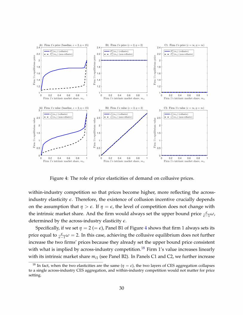
Figure 4: The role of price elasticities of demand on collusive prices.

within-industry competition so that prices become higher, more reflecting the across-industry elasticity ε. Therefore, the existence of collusion incentive crucially dependson the assumption that η > ε. If η = ε, the level of competition does not change withthe intrinsic market share. And the firm would always set the upper bound price ε

ε−1 ω,determined by the across-industry elasticity ε.

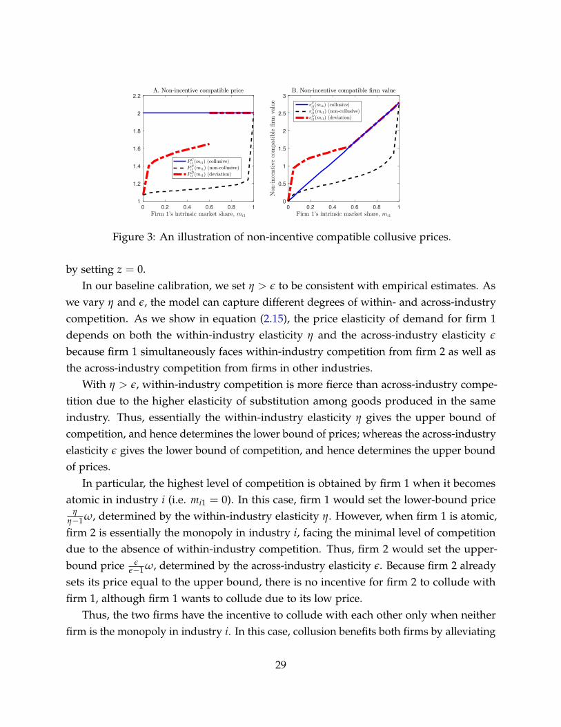
Specifically, if we set η = 2 (= ε), Panel B1 of Figure 4 shows that firm 1 always sets itsprice equal to ε

ε−1 ω = 2. In this case, achieving the collusive equilibrium does not furtherincrease the two firms’ prices because they already set the upper bound price consistentwith what is implied by across-industry competition.18 Firm 1’s value increases linearlywith its intrinsic market share mi1 (see Panel B2). In Panels C1 and C2, we further increase

18 In fact, when the two elasticities are the same (η = ε), the two layers of CES aggregation collapsesto a single across-industry CES aggregation, and within-industry competition would not matter for pricesetting.

30

η = ε = ∞ to mimic an economy with perfect competition. The infinite elasticity resultsin zero markups. Both firms set their prices equal to the marginal costs (see Panel C1)and attain zero values (see Panel C2) in equilibrium regardless of their intrinsic marketshares.

4 Main Predictions

In this section, we present the main predictions of our model. First, we show that collusiveprices are lower when the long-run consumption growth rate is low. The endogenousprice wars during periods with low long-run growth rates amplify firms’ exposure tolong-run risks. Second, we show that the industries with a larger capacity of distinctiveinnovation are less exposed to long-run risks because there are less variations in collusiveprices over long-run growth fluctuations. Thus our model implies that industries with alarger capacity of distinctive innovation are less risky. Finally, we discuss the effect oflong-run risks and antitrust enforcement on our model’s asset pricing implications.

4.1 Price Wars and Long-Run Growth Rates

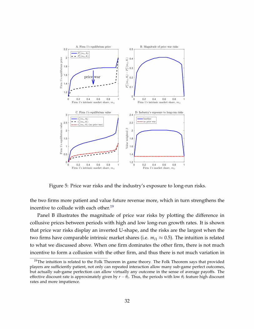
In this section, we study the endogenous change in collusive prices and firm values overbusiness cycles. Figure 5 plots firm 1’s collusive price during periods with high long-rungrowth rates (i.e. θt = θb = 0.06, blue solid line) and periods with low long-run growthrates (i.e. θt = θr = −0.06, black dashed line). We choose large differences in growth ratesfor better visualizing the channels. It is shown that the two firms collude on significantlylower prices during periods with low long-run growth rates. Thus, our model predictsthe occurrence of price wars during periods with low long-run consumption growth.

Intuitively, the incentive to collude on higher prices depends on the extent to whichthe two firms value future revenue relative to its current revenue. By deviating from thecollusive price, firms can attain higher contemporaneous revenue and accumulate morecustomer bases in the short run. However, firms run into the risk of losing future revenuebecause once the deviation is detected by the other firm, the non-collusive equilibriumwill be implemented as a punishment strategy. Switching to the non-collusive equilibriumwill be more costly when the future revenue is relatively higher, which happens duringperiods with high long-run growth rates. In fact, firms’ effective discount rate is lowerduring high long-run-growth periods due to the high growth rate in revenue. This makes

31

0 0.2 0.4 0.6 0.8 1

1.2

1.4

1.6

1.8

2

2.2

0 0.2 0.4 0.6 0.8 1

0

0.1

0.2

0.3

0.4

0.5

0 0.2 0.4 0.6 0.8 1

0

0.5

1

1.5

2

2.5

3

0 0.2 0.4 0.6 0.8 1

1.2

1.4

1.6

1.8

2

2.2

2.4

Figure 5: Price war risks and the industry’s exposure to long-run risks.

the two firms more patient and value future revenue more, which in turn strengthens theincentive to collude with each other.19

Panel B illustrates the magnitude of price war risks by plotting the difference incollusive prices between periods with high and low long-run growth rates. It is shownthat price war risks display an inverted U-shape, and the risks are the largest when thetwo firms have comparable intrinsic market shares (i.e. mi1 ≈ 0.5). The intuition is relatedto what we discussed above. When one firm dominates the other firm, there is not muchincentive to form a collusion with the other firm, and thus there is not much variation in

19The intuition is related to the Folk Theorem in game theory. The Folk Theorem says that providedplayers are sufficiently patient, not only can repeated interaction allow many sub-game perfect outcomes,but actually sub-game perfection can allow virtually any outcome in the sense of average payoffs. Theeffective discount rate is approximately given by r− θt. Thus, the periods with low θt feature high discountrates and more impatience.

32

collusive prices when long-run growth rates change.The time-varying collusion incentive amplifies the effect of long-run risks, making

firms riskier. In Panel C, the blue solid line and the black dashed line plot firm 1’s valueduring periods with high long-run growth rates (θt = θb) and periods with low long-rungrowth rates (θt = θr). Firms have significantly lower values during periods with lowlong-run growth rates due to low growth rates and low product prices. Different fromcanonical long-run-risk models, our model emphasizes that the endogenous price warsarising from declines in long-run consumption growth further reduce firms’ cash flows,generating an amplification mechanism for the effect of adverse long-run growth shocks.This amplification effect is quantitatively important. The red-dashed line illustrates thatthe firm’s value in periods with low long-run growth rates would be 20% higher onaverage if collusive prices were the same as those in periods with high long-run growthrates.

To illustrate the industry’s exposure to long-run risks, we calculate the industry-levelbeta as value-weighted firm-level betas

βi(mi1) = ∑j=1,2

vCij(mi1, θr)

vCi1(mi1, θr) + vC

i2(mi1, θr)βij(mi1), (4.1)

whereβij(mi1) = vC

ij(mi1, θb)/vCij(mi1, θr)− 1. (4.2)

The blue solid line in Panel D plots industry i’s beta when firm 1’s market sharemi1 varies. It shows that the industry’s exposure to long-run risks displays an invertedU-shape due to the inverted-U price war risks (see Panel B). As a benchmark, the reddash-dotted line plots the industry’s exposure to long-run risks in the absence of pricewar risks (i.e. when collusive prices do not change with long-run growth rates). It isshown that when the two firms have comparable intrinsic market shares, the price warrisks significantly amplify the industry’s exposure to long-run risks, increasing the valueof beta by about 50%, from 1.35 to 2.

4.2 Distinctive Innovation and the Exposure to Long-Run Risks

In this section, we study the implication of distinctive innovation on collusive prices andfirm values. We consider two industries different in the units of distinctive R&D projects.

33

0 0.2 0.4 0.6 0.8 1

1

1.2

1.4

1.6

1.8

2

2.2

0 0.2 0.4 0.6 0.8 1

0

0.5

1

1.5

2

2.5

3

0 0.2 0.4 0.6 0.8 1

1.4

1.6

1.8

2

2.2

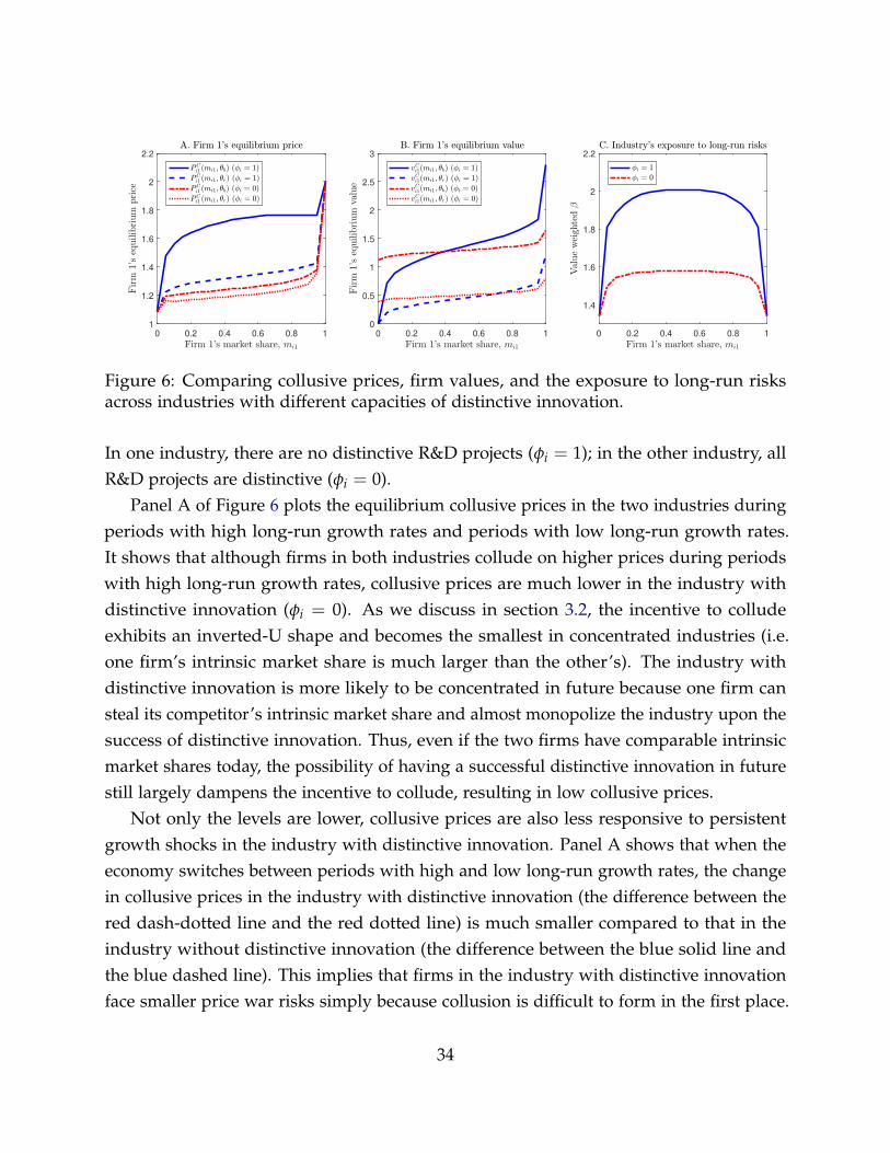
Figure 6: Comparing collusive prices, firm values, and the exposure to long-run risksacross industries with different capacities of distinctive innovation.

In one industry, there are no distinctive R&D projects (φi = 1); in the other industry, allR&D projects are distinctive (φi = 0).

Panel A of Figure 6 plots the equilibrium collusive prices in the two industries duringperiods with high long-run growth rates and periods with low long-run growth rates.It shows that although firms in both industries collude on higher prices during periodswith high long-run growth rates, collusive prices are much lower in the industry withdistinctive innovation (φi = 0). As we discuss in section 3.2, the incentive to colludeexhibits an inverted-U shape and becomes the smallest in concentrated industries (i.e.one firm’s intrinsic market share is much larger than the other’s). The industry withdistinctive innovation is more likely to be concentrated in future because one firm cansteal its competitor’s intrinsic market share and almost monopolize the industry upon thesuccess of distinctive innovation. Thus, even if the two firms have comparable intrinsicmarket shares today, the possibility of having a successful distinctive innovation in futurestill largely dampens the incentive to collude, resulting in low collusive prices.

Not only the levels are lower, collusive prices are also less responsive to persistentgrowth shocks in the industry with distinctive innovation. Panel A shows that when theeconomy switches between periods with high and low long-run growth rates, the changein collusive prices in the industry with distinctive innovation (the difference between thered dash-dotted line and the red dotted line) is much smaller compared to that in theindustry without distinctive innovation (the difference between the blue solid line andthe blue dashed line). This implies that firms in the industry with distinctive innovationface smaller price war risks simply because collusion is difficult to form in the first place.

34

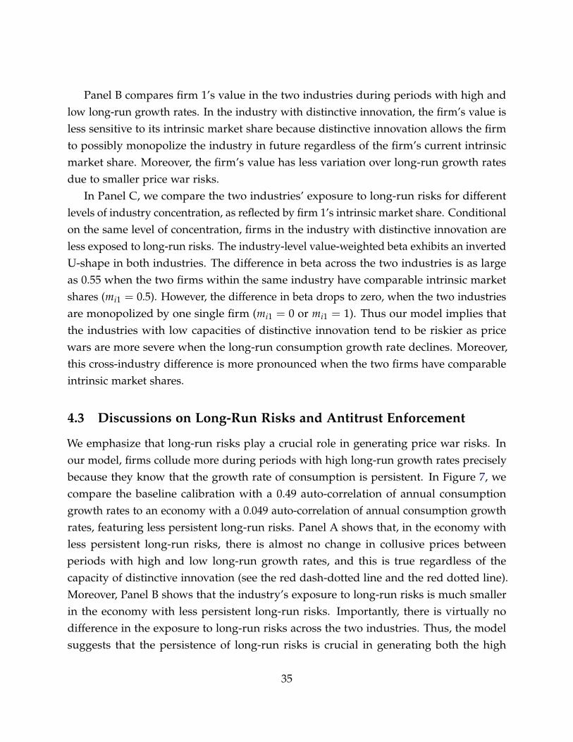
Panel B compares firm 1’s value in the two industries during periods with high andlow long-run growth rates. In the industry with distinctive innovation, the firm’s value isless sensitive to its intrinsic market share because distinctive innovation allows the firmto possibly monopolize the industry in future regardless of the firm’s current intrinsicmarket share. Moreover, the firm’s value has less variation over long-run growth ratesdue to smaller price war risks.

In Panel C, we compare the two industries’ exposure to long-run risks for differentlevels of industry concentration, as reflected by firm 1’s intrinsic market share. Conditionalon the same level of concentration, firms in the industry with distinctive innovation areless exposed to long-run risks. The industry-level value-weighted beta exhibits an invertedU-shape in both industries. The difference in beta across the two industries is as largeas 0.55 when the two firms within the same industry have comparable intrinsic marketshares (mi1 = 0.5). However, the difference in beta drops to zero, when the two industriesare monopolized by one single firm (mi1 = 0 or mi1 = 1). Thus our model implies thatthe industries with low capacities of distinctive innovation tend to be riskier as pricewars are more severe when the long-run consumption growth rate declines. Moreover,this cross-industry difference is more pronounced when the two firms have comparableintrinsic market shares.

4.3 Discussions on Long-Run Risks and Antitrust Enforcement

We emphasize that long-run risks play a crucial role in generating price war risks. Inour model, firms collude more during periods with high long-run growth rates preciselybecause they know that the growth rate of consumption is persistent. In Figure 7, wecompare the baseline calibration with a 0.49 auto-correlation of annual consumptiongrowth rates to an economy with a 0.049 auto-correlation of annual consumption growthrates, featuring less persistent long-run risks. Panel A shows that, in the economy withless persistent long-run risks, there is almost no change in collusive prices betweenperiods with high and low long-run growth rates, and this is true regardless of thecapacity of distinctive innovation (see the red dash-dotted line and the red dotted line).Moreover, Panel B shows that the industry’s exposure to long-run risks is much smallerin the economy with less persistent long-run risks. Importantly, there is virtually nodifference in the exposure to long-run risks across the two industries. Thus, the modelsuggests that the persistence of long-run risks is crucial in generating both the high

35

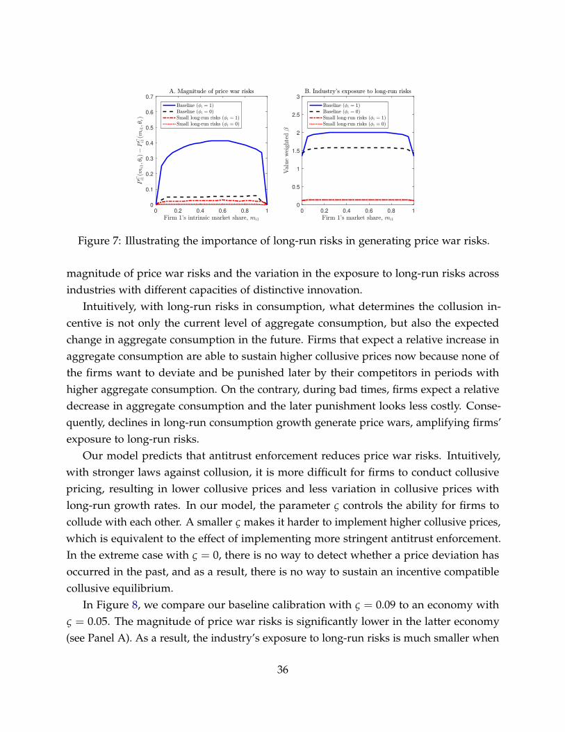
0 0.2 0.4 0.6 0.8 1

0

0.1

0.2

0.3

0.4

0.5

0.6

0.7

0 0.2 0.4 0.6 0.8 1

0

0.5

1

1.5

2

2.5

3

Figure 7: Illustrating the importance of long-run risks in generating price war risks.

magnitude of price war risks and the variation in the exposure to long-run risks acrossindustries with different capacities of distinctive innovation.

Intuitively, with long-run risks in consumption, what determines the collusion in-centive is not only the current level of aggregate consumption, but also the expectedchange in aggregate consumption in the future. Firms that expect a relative increase inaggregate consumption are able to sustain higher collusive prices now because none ofthe firms want to deviate and be punished later by their competitors in periods withhigher aggregate consumption. On the contrary, during bad times, firms expect a relativedecrease in aggregate consumption and the later punishment looks less costly. Conse-quently, declines in long-run consumption growth generate price wars, amplifying firms’exposure to long-run risks.

Our model predicts that antitrust enforcement reduces price war risks. Intuitively,with stronger laws against collusion, it is more difficult for firms to conduct collusivepricing, resulting in lower collusive prices and less variation in collusive prices withlong-run growth rates. In our model, the parameter ς controls the ability for firms tocollude with each other. A smaller ς makes it harder to implement higher collusive prices,which is equivalent to the effect of implementing more stringent antitrust enforcement.In the extreme case with ς = 0, there is no way to detect whether a price deviation hasoccurred in the past, and as a result, there is no way to sustain an incentive compatiblecollusive equilibrium.

In Figure 8, we compare our baseline calibration with ς = 0.09 to an economy withς = 0.05. The magnitude of price war risks is significantly lower in the latter economy(see Panel A). As a result, the industry’s exposure to long-run risks is much smaller when

36

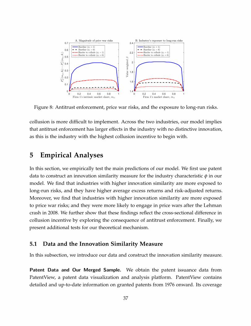
0 0.2 0.4 0.6 0.8 1

0

0.1

0.2

0.3

0.4

0.5

0.6

0.7

0 0.2 0.4 0.6 0.8 1

1.4

1.6

1.8

2

2.2

2.4

Figure 8: Antitrust enforcement, price war risks, and the exposure to long-run risks.

collusion is more difficult to implement. Across the two industries, our model impliesthat antitrust enforcement has larger effects in the industry with no distinctive innovation,as this is the industry with the highest collusion incentive to begin with.

5 Empirical Analyses

In this section, we empirically test the main predictions of our model. We first use patentdata to construct an innovation similarity measure for the industry characteristic φ in ourmodel. We find that industries with higher innovation similarity are more exposed tolong-run risks, and they have higher average excess returns and risk-adjusted returns.Moreover, we find that industries with higher innovation similarity are more exposedto price war risks; and they were more likely to engage in price wars after the Lehmancrash in 2008. We further show that these findings reflect the cross-sectional difference incollusion incentive by exploring the consequence of antitrust enforcement. Finally, wepresent additional tests for our theoretical mechanism.

5.1 Data and the Innovation Similarity Measure

In this subsection, we introduce our data and construct the innovation similarity measure.

Patent Data and Our Merged Sample. We obtain the patent issuance data fromPatentView, a patent data visualization and analysis platform. PatentView containsdetailed and up-to-date information on granted patents from 1976 onward. Its coverage

37

of recent patenting activities is more comprehensive than the NBER patent data (Hall,Jaffe and Trajtenberg, 2001) and the patent data assembled by Kogan et al. (2017).20

Patent assignees in PatentView are disambiguated and their locations and patenting ac-tivities are longitudinally tracked. PatentView categorizes patent assignees into differentgroups, such as corporations, individuals, and government agencies. It also providesdetailed information of individual patents, including their grant dates and technologyclassifications.

We match patent assignees in PatentView to U.S. public firms in CRSP/Compustat,and to U.S. private firms and foreign firms in Capital IQ.21 We drop patents granted toindividuals and government agencies. We include private firms in our sample becausethey play an important role in industry competition (see e.g. Ali, Klasa and Yeung, 2008).

We use a fuzzy name-matching algorithm to obtain a pool of potential matches fromCRSP/Compustat and Capital IQ for each patent assignee in PatentView. We thenmanually screen these potential matches to identify the exact matches based on patentassignees’ names and addresses. In Appendix B.2, we detail our matching procedure. Intotal, we match 2, 235, 201 patents to 10, 139 U.S. public firms, 132, 100 patents to 3, 080U.S. private firms, 241, 582 patents to 300 foreign public firms, and 35, 597 patents to285 foreign private firms.22 The merged sample covers 13, 804 firms in 752 4-digit SICindustries from 1976 to 2017.23

Innovation Similarity Measure. We construct our innovation similarity measure (de-noted as “innosimm”) for the industry-level innovation similarity based on the technologyclassifications of an industry’s patents. In light of previous studies (e.g. Jaffe, 1986; Bloom,Schankerman and Van Reenen, 2013), we measure the cosine similarity of two patentswithin the same industry based on their technology classification vectors.24 Specifically,

20The PatentView data contain all patents granted by the U.S. Patent and Trademark Office (USPTO)from 1976 to 2017, while the NBER data and the data used by Kogan et al. (2017) only cover patents grantedup to 2006 and 2010, respectively.

21Capital IQ is one of the most comprehensive data that include private firms and foreign firms.22Our empirical results remain robust if we confine the patent data to those granted to U.S. public firms.23We use 4-digit SIC codes in Compustat and Capital IQ to identify the industries of patent assignees.

Both Compustat and Capital IQ are developed and maintained by S&P Global and the SIC industryclassifications in these two datasets are consistent with each other. We verify the consistency by comparingthe SIC codes for U.S. public firms covered by both Compustat and Capital IQ. We find that the SIC codesof these firms are virtually identical across the two data sources.

24PatentView provides both the Cooperative Patent Classification (CPC) and the U.S. Patent Classification(USPC), the two major classification systems for U.S. patents. We use CPC for our analyses because USPC

38

the similarity between two patents, a and b, is defined by:

similarity (a, b) =A · B‖A‖ ‖B‖ , (5.1)

where A and B are the technology vectors of patent a and patent b. If the two patents shareexactly the same technology classifications, the cosine similarity attains the maximumvalue, 1. If the two patents are mutually exclusive in their technology classifications, thecosine similarity reaches the minimum value, 0. Because patent technology classificationsare assigned according to the technical features of patents, the cosine similarity measurecaptures how similar the patents are in terms of their technological positions. Based onthe pairwise cosine similarity of patents, we take the following steps to construct theindustry-level innovation similarity measure.

First, we construct the patent-level similarity measure to capture to what extent apatent is differentiated from other patents recently developed by peer firms. In particular,for a patent granted to firm i in year t, the patent-level similarity measure is the averageof the pairwise cosine similarity (defined by equation 5.1) between this patent and theother patents granted to firm i’s peer firms in the same 4-digit SIC industry from yeart− 5 to year t− 1.

Next, we aggregate patent-level similarity measures to obtain industry-level similaritymeasures. For example, a 4-digit SIC industry’s similarity measure in year t is theaverage of patent-level similarity measures associated with all the patents granted tofirms in the industry in year t. Because firms are not granted with patents every year, wefurther average the industry-level similarity measures over time to filter noise and bettercapture firms’ ability in generating differentiated innovations. In particular, our innosimmmeasure in industry i and year t (i.e. innosimmit) is constructed as the time-series averageof industry i’s similarity measures from year t− 9 to year t.

Panel A of Figure 9 presents the time-series of several industries’ innosimm measure.In the “Search, Detection, Navigation, Guidance, Aeronautical, and Nautical Systemsand Instruments” industry, the innosimm measure is low throughout our sample period,suggesting that firms in this industry seem to be able to consistently generate distinctiveinnovation. The innosimm measure keeps increasing for the “Drilling Oil and Gas Wells”

is not available after 2015. Our results are robust to the classification based on USPC for data prior to 2015.There are 653 unique CPC classes in PatentView. The technology classification vector for a patent consistsof 653 indicator variables that represent the patent’s CPC classes.

39

industry, while it peaks in year 2000 for the “Rubber and Plastics Footwear.” industry.

Validation of the Innosimm Measure. We conduct one external validation for ourinnosimm measure. If a higher innosimm captures a lower capacity of distinctive in-novation in an industry, we expect that fewer consumers would consider the brandsof high-innosimm industries as distinctive. We test this hypothesis by examining therelation between innosimm and the relative change in brand distinctiveness over time,measured using the BAV consumer survey data.25 We standardize innosimm using itsunconditional mean and the standard deviation of all industries’ innosimm across alltime to ease the interpretation of coefficients in our regression analyses. Column (1) ofTable 1 shows that innosimm is negatively correlated with the two-year percent change inthe industry-level brand distinctiveness, suggesting that industries with higher innosimmare associated with lower brand distinctiveness in future.

Our innosimm measure is conceptually different from the product similarity measure(denoted as “prodsimm”) constructed by Hoberg and Phillips (2016). Innosimm capturesto what extent firms in an industry can differentiate their products from peers’ throughinnovation. Thus, it is a forward-looking measure that captures the (potential) similar-ity/distinctiveness of firms’ businesses in the future. Product similarity, on the other hand,is derived from text analyses based on firms’ current product description (Hoberg andPhillips, 2016). Therefore, it reflects the similarity of products produced by different firmsas of today, rather than the potential similarity/distinctiveness of firms’ products in thefuture. In other words, product similarity contains littile information, if at all, about firms’innovation activities, which are the necessary inputs for making products distinctive inthe future. The conceptual difference between the two measures is formally confirmed bycolumn (2) of Table 1, which shows that innosimm is unrelated with product similarity.26

In Section 5.2 and 5.3, we further show that the product similarity measure is neitherpriced in the cross section nor related to industries’ price war risks.

25The BAV database is regarded as the world’s most comprehensive database of consumers’ perceptionof brands (see, e.g. Gerzema and Lebar, 2008; Keller, 2008; Mizik and Jacobson, 2008; Aaker, 2012; Lovett,Peres and Shachar, 2014; Tavassoli, Sorescu and Chandy, 2014). The BAV brand perception survey consistsof more than 870,000 respondents in total, and it is constructed to represent the U.S. population accordingto gender, ethnicity, age, income group, and geographic location. See Dou et al. (2018) for the details of thesurvey.

26The correlation between product similarity and innosimm is low. The Pearson correlation coefficient,the Spearman’s rank correlation coefficient, and the Kendall’s τA and τB coefficients between the twovariables are 0.06, 0.02, 0.04, and 0.04, respectively.

40

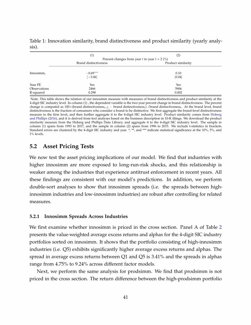
Table 1: Innovation similarity, brand distinctiveness and product similarity (yearly analy-sis).

(1) (2)Percent changes from year t to year t + 2 (%)

Brand distinctiveness Product similarity

Innosimmt −0.69∗∗∗ 0.10[−3.06] [0.04]

Year FE Yes YesObservations 2466 5906R-squared 0.298 0.002

Note: This table shows the relation of our innosimm measure with measures of brand distinctiveness and product similarity at the4-digit SIC industry level. In column (1) , the dependent variable is the two-year percent change in brand distinctiveness. The percentchange is computed as 100×(brand distinctivenesst+2 − brand distinctivenesst) /brand distinctivenesst. At the brand level, branddistinctiveness is the fraction of consumers who consider a brand to be distinctive. We first aggregate the brand-level distinctivenessmeasure to the firm level, and then further aggregate it to the 4-digit SIC industry level. Product similarity comes from Hobergand Phillips (2016), and it is derived from text analyses based on the business description in 10-K filings. We download the productsimilarity measure from the Hoberg and Phillips Data Library, and aggregate it to the 4-digit SIC industry level. The sample incolumn (1) spans from 1993 to 2017, and the sample in column (2) spans from 1996 to 2015. We include t-statistics in brackets.Standard errors are clustered by the 4-digit SIC industry and year. *, **, and *** indicate statistical significance at the 10%, 5%, and1% levels.

5.2 Asset Pricing Tests

We now test the asset pricing implications of our model. We find that industries withhigher innosimm are more exposed to long-run-risk shocks, and this relationship isweaker among the industries that experience antitrust enforcement in recent years. Allthese findings are consistent with our model’s predictions. In addition, we performdouble-sort analyses to show that innosimm spreads (i.e. the spreads between high-innosimm industries and low-innosimm industries) are robust after controlling for relatedmeasures.

5.2.1 Innosimm Spreads Across Industries

We first examine whether innosimm is priced in the cross section. Panel A of Table 2presents the value-weighted average excess returns and alphas for the 4-digit SIC industryportfolios sorted on innosimm. It shows that the portfolio consisting of high-innosimmindustries (i.e. Q5) exhibits significantly higher average excess returns and alphas. Thespread in average excess returns between Q1 and Q5 is 3.41% and the spreads in alphasrange from 4.75% to 9.24% across different factor models.

Next, we perform the same analysis for prodsimm. We find that prodsimm is notpriced in the cross section. The return difference between the high-prodsimm portfolio

41

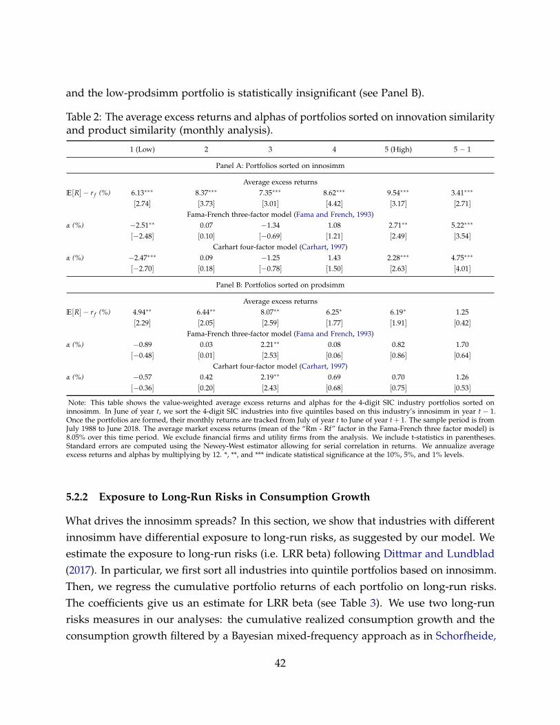
and the low-prodsimm portfolio is statistically insignificant (see Panel B).

Table 2: The average excess returns and alphas of portfolios sorted on innovation similarityand product similarity (monthly analysis).

1 (Low) 2 3 4 5 (High) 5 − 1

Panel A: Portfolios sorted on innosimm

Average excess returnsE[R]− r f (%) 6.13∗∗∗ 8.37∗∗∗ 7.35∗∗∗ 8.62∗∗∗ 9.54∗∗∗ 3.41∗∗∗

[2.74] [3.73] [3.01] [4.42] [3.17] [2.71]Fama-French three-factor model (Fama and French, 1993)

α (%) −2.51∗∗ 0.07 −1.34 1.08 2.71∗∗ 5.22∗∗∗

[−2.48] [0.10] [−0.69] [1.21] [2.49] [3.54]Carhart four-factor model (Carhart, 1997)

α (%) −2.47∗∗∗ 0.09 −1.25 1.43 2.28∗∗∗ 4.75∗∗∗

[−2.70] [0.18] [−0.78] [1.50] [2.63] [4.01]

Panel B: Portfolios sorted on prodsimm

Average excess returnsE[R]− r f (%) 4.94∗∗ 6.44∗∗ 8.07∗∗ 6.25∗ 6.19∗ 1.25

[2.29] [2.05] [2.59] [1.77] [1.91] [0.42]Fama-French three-factor model (Fama and French, 1993)

α (%) −0.89 0.03 2.21∗∗ 0.08 0.82 1.70[−0.48] [0.01] [2.53] [0.06] [0.86] [0.64]

Carhart four-factor model (Carhart, 1997)α (%) −0.57 0.42 2.19∗∗ 0.69 0.70 1.26

[−0.36] [0.20] [2.43] [0.68] [0.75] [0.53]

Note: This table shows the value-weighted average excess returns and alphas for the 4-digit SIC industry portfolios sorted oninnosimm. In June of year t, we sort the 4-digit SIC industries into five quintiles based on this industry’s innosimm in year t− 1.Once the portfolios are formed, their monthly returns are tracked from July of year t to June of year t + 1. The sample period is fromJuly 1988 to June 2018. The average market excess returns (mean of the “Rm - Rf” factor in the Fama-French three factor model) is8.05% over this time period. We exclude financial firms and utility firms from the analysis. We include t-statistics in parentheses.Standard errors are computed using the Newey-West estimator allowing for serial correlation in returns. We annualize averageexcess returns and alphas by multiplying by 12. *, **, and *** indicate statistical significance at the 10%, 5%, and 1% levels.

5.2.2 Exposure to Long-Run Risks in Consumption Growth

What drives the innosimm spreads? In this section, we show that industries with differentinnosimm have differential exposure to long-run risks, as suggested by our model. Weestimate the exposure to long-run risks (i.e. LRR beta) following Dittmar and Lundblad(2017). In particular, we first sort all industries into quintile portfolios based on innosimm.Then, we regress the cumulative portfolio returns of each portfolio on long-run risks.The coefficients give us an estimate for LRR beta (see Table 3). We use two long-runrisks measures in our analyses: the cumulative realized consumption growth and theconsumption growth filtered by a Bayesian mixed-frequency approach as in Schorfheide,

42

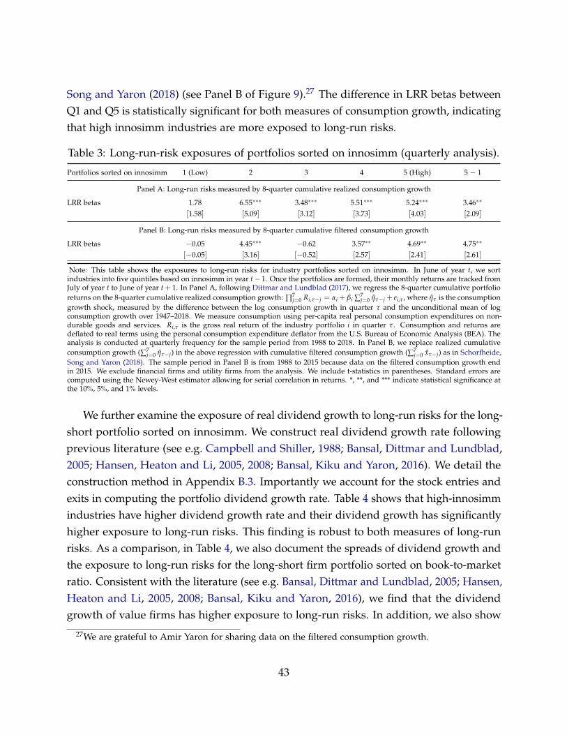
Song and Yaron (2018) (see Panel B of Figure 9).27 The difference in LRR betas betweenQ1 and Q5 is statistically significant for both measures of consumption growth, indicatingthat high innosimm industries are more exposed to long-run risks.

Table 3: Long-run-risk exposures of portfolios sorted on innosimm (quarterly analysis).

Portfolios sorted on innosimm 1 (Low) 2 3 4 5 (High) 5 − 1

Panel A: Long-run risks measured by 8-quarter cumulative realized consumption growth

LRR betas 1.78 6.55∗∗∗ 3.48∗∗∗ 5.51∗∗∗ 5.24∗∗∗ 3.46∗∗

[1.58] [5.09] [3.12] [3.73] [4.03] [2.09]

Panel B: Long-run risks measured by 8-quarter cumulative filtered consumption growth

LRR betas −0.05 4.45∗∗∗ −0.62 3.57∗∗ 4.69∗∗ 4.75∗∗

[−0.05] [3.16] [−0.52] [2.57] [2.41] [2.61]

Note: This table shows the exposures to long-run risks for industry portfolios sorted on innosimm. In June of year t, we sortindustries into five quintiles based on innosimm in year t− 1. Once the portfolios are formed, their monthly returns are tracked fromJuly of year t to June of year t + 1. In Panel A, following Dittmar and Lundblad (2017), we regress the 8-quarter cumulative portfolioreturns on the 8-quarter cumulative realized consumption growth: ∏7

j=0 Ri,τ−j = αi + βi ∑7j=0 ητ−j + ei,τ , where ητ is the consumption

growth shock, measured by the difference between the log consumption growth in quarter τ and the unconditional mean of logconsumption growth over 1947–2018. We measure consumption using per-capita real personal consumption expenditures on non-durable goods and services. Ri,τ is the gross real return of the industry portfolio i in quarter τ. Consumption and returns aredeflated to real terms using the personal consumption expenditure deflator from the U.S. Bureau of Economic Analysis (BEA). Theanalysis is conducted at quarterly frequency for the sample period from 1988 to 2018. In Panel B, we replace realized cumulativeconsumption growth (∑7

j=0 ητ−j) in the above regression with cumulative filtered consumption growth (∑7j=0 xτ−j) as in Schorfheide,

Song and Yaron (2018). The sample period in Panel B is from 1988 to 2015 because data on the filtered consumption growth endin 2015. We exclude financial firms and utility firms from the analysis. We include t-statistics in parentheses. Standard errors arecomputed using the Newey-West estimator allowing for serial correlation in returns. *, **, and *** indicate statistical significance atthe 10%, 5%, and 1% levels.

We further examine the exposure of real dividend growth to long-run risks for the long-short portfolio sorted on innosimm. We construct real dividend growth rate followingprevious literature (see e.g. Campbell and Shiller, 1988; Bansal, Dittmar and Lundblad,2005; Hansen, Heaton and Li, 2005, 2008; Bansal, Kiku and Yaron, 2016). We detail theconstruction method in Appendix B.3. Importantly we account for the stock entries andexits in computing the portfolio dividend growth rate. Table 4 shows that high-innosimmindustries have higher dividend growth rate and their dividend growth has significantlyhigher exposure to long-run risks. This finding is robust to both measures of long-runrisks. As a comparison, in Table 4, we also document the spreads of dividend growth andthe exposure to long-run risks for the long-short firm portfolio sorted on book-to-marketratio. Consistent with the literature (see e.g. Bansal, Dittmar and Lundblad, 2005; Hansen,Heaton and Li, 2005, 2008; Bansal, Kiku and Yaron, 2016), we find that the dividendgrowth of value firms has higher exposure to long-run risks. In addition, we also show

27We are grateful to Amir Yaron for sharing data on the filtered consumption growth.

43

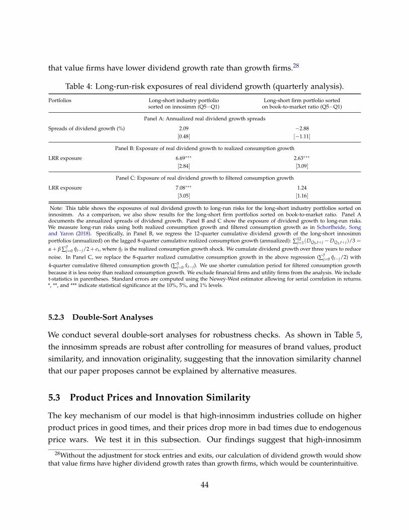
that value firms have lower dividend growth rate than growth firms.28

Table 4: Long-run-risk exposures of real dividend growth (quarterly analysis).

Portfolios Long-short industry portfoliosorted on innosimm (Q5−Q1)

Long-short firm portfolio sortedon book-to-market ratio (Q5−Q1)

Panel A: Annualized real dividend growth spreads

Spreads of dividend growth (%) 2.09 −2.88[0.48] [−1.11]

Panel B: Exposure of real dividend growth to realized consumption growth

LRR exposure 6.69∗∗∗ 2.63∗∗∗

[2.84] [3.09]

Panel C: Exposure of real dividend growth to filtered consumption growth

LRR exposure 7.08∗∗∗ 1.24[3.05] [1.16]

Note: This table shows the exposures of real dividend growth to long-run risks for the long-short industry portfolios sorted oninnosimm. As a comparison, we also show results for the long-short firm portfolios sorted on book-to-market ratio. Panel Adocuments the annualized spreads of dividend growth. Panel B and C show the exposure of dividend growth to long-run risks.We measure long-run risks using both realized consumption growth and filtered consumption growth as in Schorfheide, Songand Yaron (2018). Specifically, in Panel B, we regress the 12-quarter cumulative dividend growth of the long-short innosimmportfolios (annualized) on the lagged 8-quarter cumulative realized consumption growth (annualized): ∑12

j=1(DQ5 ,t+j −DQ1 ,t+j)/3 =

α + β ∑7j=0 ηt−j/2+ et, where ηt is the realized consumption growth shock. We cumulate dividend growth over three years to reduce

noise. In Panel C, we replace the 8-quarter realized cumulative consumption growth in the above regression (∑7j=0 ηt−j/2) with

4-quarter cumulative filtered consumption growth (∑3j=0 xt−j). We use shorter cumulation period for filtered consumption growth

because it is less noisy than realized consumption growth. We exclude financial firms and utility firms from the analysis. We includet-statistics in parentheses. Standard errors are computed using the Newey-West estimator allowing for serial correlation in returns.*, **, and *** indicate statistical significance at the 10%, 5%, and 1% levels.

5.2.3 Double-Sort Analyses

We conduct several double-sort analyses for robustness checks. As shown in Table 5,the innosimm spreads are robust after controlling for measures of brand values, productsimilarity, and innovation originality, suggesting that the innovation similarity channelthat our paper proposes cannot be explained by alternative measures.

5.3 Product Prices and Innovation Similarity

The key mechanism of our model is that high-innosimm industries collude on higherproduct prices in good times, and their prices drop more in bad times due to endogenousprice wars. We test it in this subsection. Our findings suggest that high-innosimm

28Without the adjustment for stock entries and exits, our calculation of dividend growth would showthat value firms have higher dividend growth rates than growth firms, which would be counterintuitive.

44

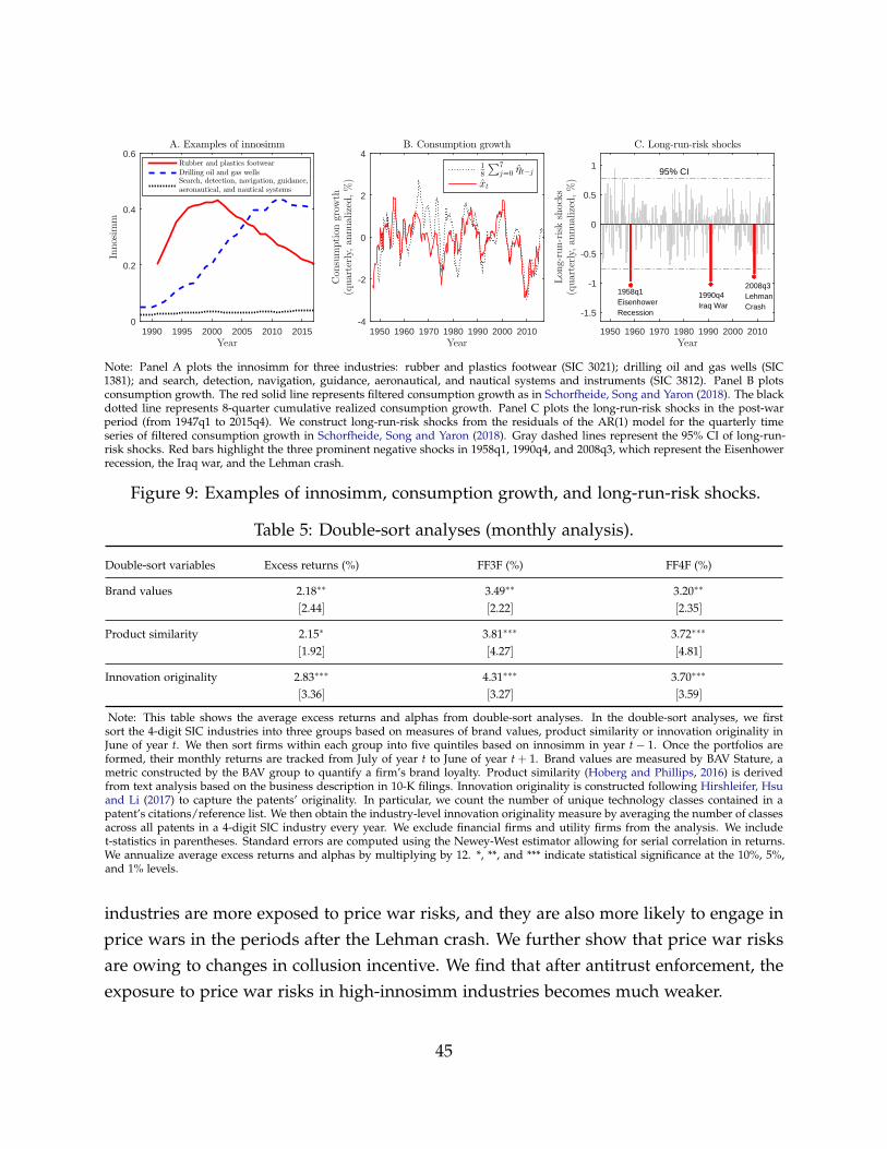
Year1990 1995 2000 2005 2010 2015

Innosim

m

0

0.2

0.4

0.6A. Examples of innosimm

Rubber and plastics footwearDrilling oil and gas wellsSearch, detection, navigation, guidance,aeronautical, and nautical systems

Year1950 1960 1970 1980 1990 2000 2010

Con

sumption

grow

th(quarterly,

annualized,%)

-4

-2

0

2

4B. Consumption growth

18

∑7j=0 ηt−j

xt

Year1950 1960 1970 1980 1990 2000 2010

Lon

g-run-riskshocks

(quarterly,

annualized,%)

-1.5

-1

-0.5

0

0.5

1

1958q1EisenhowerRecession

1990q4Iraq War

2008q3LehmanCrash

95% CI

C. Long-run-risk shocks

Note: Panel A plots the innosimm for three industries: rubber and plastics footwear (SIC 3021); drilling oil and gas wells (SIC1381); and search, detection, navigation, guidance, aeronautical, and nautical systems and instruments (SIC 3812). Panel B plotsconsumption growth. The red solid line represents filtered consumption growth as in Schorfheide, Song and Yaron (2018). The blackdotted line represents 8-quarter cumulative realized consumption growth. Panel C plots the long-run-risk shocks in the post-warperiod (from 1947q1 to 2015q4). We construct long-run-risk shocks from the residuals of the AR(1) model for the quarterly timeseries of filtered consumption growth in Schorfheide, Song and Yaron (2018). Gray dashed lines represent the 95% CI of long-run-risk shocks. Red bars highlight the three prominent negative shocks in 1958q1, 1990q4, and 2008q3, which represent the Eisenhowerrecession, the Iraq war, and the Lehman crash.

Figure 9: Examples of innosimm, consumption growth, and long-run-risk shocks.

Table 5: Double-sort analyses (monthly analysis).

Double-sort variables Excess returns (%) FF3F (%) FF4F (%)

Brand values 2.18∗∗ 3.49∗∗ 3.20∗∗

[2.44] [2.22] [2.35]

Product similarity 2.15∗ 3.81∗∗∗ 3.72∗∗∗

[1.92] [4.27] [4.81]

Innovation originality 2.83∗∗∗ 4.31∗∗∗ 3.70∗∗∗

[3.36] [3.27] [3.59]

Note: This table shows the average excess returns and alphas from double-sort analyses. In the double-sort analyses, we firstsort the 4-digit SIC industries into three groups based on measures of brand values, product similarity or innovation originality inJune of year t. We then sort firms within each group into five quintiles based on innosimm in year t− 1. Once the portfolios areformed, their monthly returns are tracked from July of year t to June of year t + 1. Brand values are measured by BAV Stature, ametric constructed by the BAV group to quantify a firm’s brand loyalty. Product similarity (Hoberg and Phillips, 2016) is derivedfrom text analysis based on the business description in 10-K filings. Innovation originality is constructed following Hirshleifer, Hsuand Li (2017) to capture the patents’ originality. In particular, we count the number of unique technology classes contained in apatent’s citations/reference list. We then obtain the industry-level innovation originality measure by averaging the number of classesacross all patents in a 4-digit SIC industry every year. We exclude financial firms and utility firms from the analysis. We includet-statistics in parentheses. Standard errors are computed using the Newey-West estimator allowing for serial correlation in returns.We annualize average excess returns and alphas by multiplying by 12. *, **, and *** indicate statistical significance at the 10%, 5%,and 1% levels.

industries are more exposed to price war risks, and they are also more likely to engage inprice wars in the periods after the Lehman crash. We further show that price war risksare owing to changes in collusion incentive. We find that after antitrust enforcement, theexposure to price war risks in high-innosimm industries becomes much weaker.

45

5.3.1 The Nielsen Data for Product Prices

We use the Nielsen Retail Measurement Services scanner data to measure product pricechanges.29 The Nielsen data record prices and quantities of every unique product thathad any sales in the 42, 928 stores of more than 90 retail chains in the U.S. market fromJanuary 2006 to December 2016. In total, the Nielsen data consist of more than 3.5 millionunique products identified by the Universal Product Codes (UPCs), and the data represent53% of all sales in grocery stores, 55% in drug stores, 32% in mass merchandisers, 2%in convenience stores, and 1% in liquor stores (see e.g. Argente, Lee and Moreira, 2018).We use the product-firm links provided by GS1, the official source of UPCs in the U.S.,to match products in the Nielsen data to firms in CRSP/Compustat and Capital IQ. InAppendix B.4, we detail the matching procedure. Our merged data cover the productprices of 472 4-digit SIC industries.

5.3.2 Product Prices around the Lehman Crash

To begin, we examine the changes in product prices around the Lenman crash, the periodduring which the U.S. economy experienced a prominent negative long-run-risk shock(see Panel C of Figure 9). We sort all industries into tertiles based on innosimm. Table6 quantifies the changes in product prices among high-innosimm industries (Tertile 3)relative to low-innosimm industries (Tertile 1) around the Lehman crash. In particular, werestrict the sample to industries in Tertile 1 and Tertile 3, and create a Tertile-3 indicator forthe latter group. We also create a post-Lehman indicator that equals one for observationsin Oct. 2008 and thereafter. We then regress the percent change in product prices on theTertile-3 indicator, the post-Lehman indicator, and an interaction term between these twoindicators. The coefficient of the interaction term is negative and statistically significantacross different regression specifications (see column 1 - 4), suggesting that productprices in high-innosimm industries reduce significantly relative to those in low-innosimmindustries after the Lehman crash. The difference in product prices is economicallysignificant. Relative to low-innosimm industries, product prices decrease by 4.98% to6.64% in high-innosimm industries after the Lehman crash.

29The Nielsen data are obtained from the Kilts Center for Marketing at the University of ChicagoBooth School of Business (https://www.chicagobooth.edu/research/kilts/datasets/nielsen). Thedata have been widely used in the macroeconomics literature (e.g. Aguiar and Hurst, 2007; Broda andWeinstein, 2010; Hottman, Redding and Weinstein, 2016; Argente, Lee and Moreira, 2018; Jaravel, 2018).

46

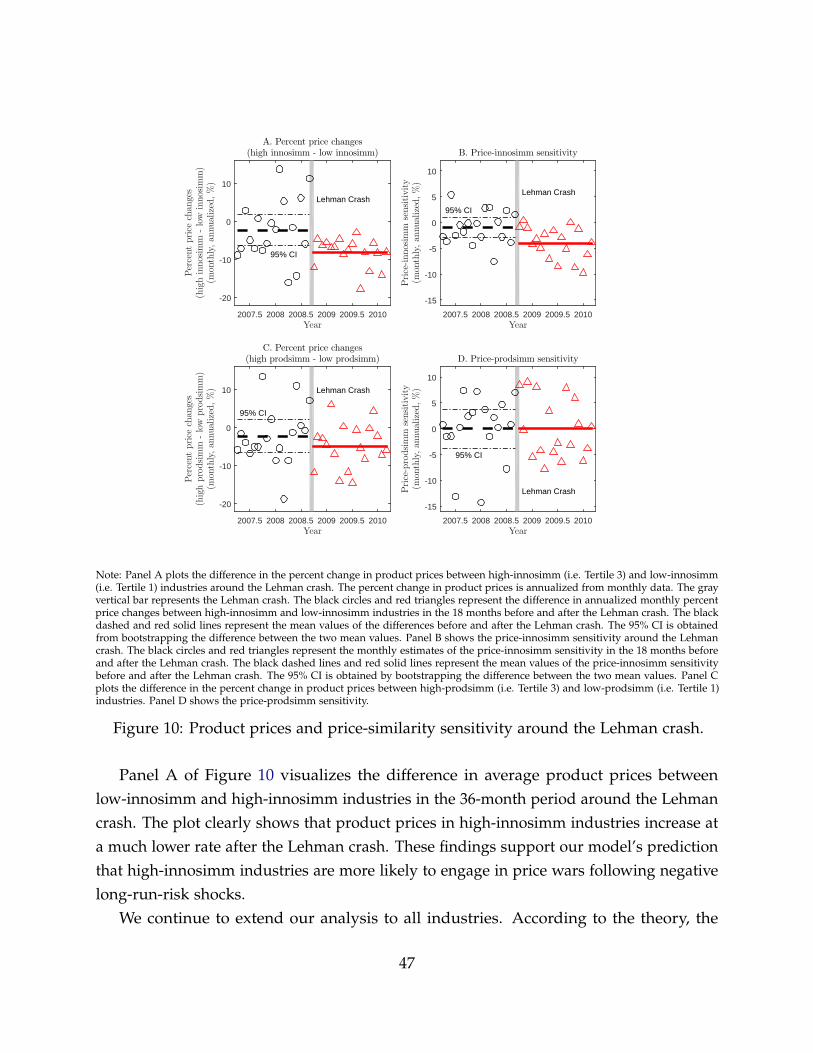
Year2007.5 2008 2008.5 2009 2009.5 2010

Percentprice

chan

ges

(highinnosim

m-low

innosim

m)

(mon

thly,an

nualized,%)

-20

-10

0

10

Lehman Crash

95% CI

A. Percent price changes(high innosimm - low innosimm)

Year2007.5 2008 2008.5 2009 2009.5 2010

Price-innosim

msensitivity

(mon

thly,an

nualized,%)

-15

-10

-5

0

5

10

Lehman Crash

95% CI

B. Price-innosimm sensitivity

Year2007.5 2008 2008.5 2009 2009.5 2010

Percentprice

chan

ges

(highprodsimm

-low

prodsimm)

(mon

thly,an

nualized,%)

-20

-10

0

10 Lehman Crash

95% CI

C. Percent price changes(high prodsimm - low prodsimm)

Year2007.5 2008 2008.5 2009 2009.5 2010

Price-prodsimm

sensitivity

(mon

thly,an

nualized,%)

-15

-10

-5

0

5

10

Lehman Crash

95% CI

D. Price-prodsimm sensitivity

Note: Panel A plots the difference in the percent change in product prices between high-innosimm (i.e. Tertile 3) and low-innosimm(i.e. Tertile 1) industries around the Lehman crash. The percent change in product prices is annualized from monthly data. The grayvertical bar represents the Lehman crash. The black circles and red triangles represent the difference in annualized monthly percentprice changes between high-innosimm and low-innosimm industries in the 18 months before and after the Lehman crash. The blackdashed and red solid lines represent the mean values of the differences before and after the Lehman crash. The 95% CI is obtainedfrom bootstrapping the difference between the two mean values. Panel B shows the price-innosimm sensitivity around the Lehmancrash. The black circles and red triangles represent the monthly estimates of the price-innosimm sensitivity in the 18 months beforeand after the Lehman crash. The black dashed lines and red solid lines represent the mean values of the price-innosimm sensitivitybefore and after the Lehman crash. The 95% CI is obtained by bootstrapping the difference between the two mean values. Panel Cplots the difference in the percent change in product prices between high-prodsimm (i.e. Tertile 3) and low-prodsimm (i.e. Tertile 1)industries. Panel D shows the price-prodsimm sensitivity.

Figure 10: Product prices and price-similarity sensitivity around the Lehman crash.

Panel A of Figure 10 visualizes the difference in average product prices betweenlow-innosimm and high-innosimm industries in the 36-month period around the Lehmancrash. The plot clearly shows that product prices in high-innosimm industries increase ata much lower rate after the Lehman crash. These findings support our model’s predictionthat high-innosimm industries are more likely to engage in price wars following negativelong-run-risk shocks.

We continue to extend our analysis to all industries. According to the theory, the

47

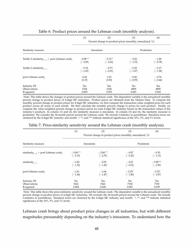
Table 6: Product prices around the Lehman crash (monthly analysis).(1) (2) (3) (4)

Percent change in product prices (monthly, annualized, %)

Similarity measure Innosimm Prodsimm

Tertile-3 similarityt−1 × post Lehman crasht −4.98∗∗∗ −5.12∗∗ −2.02 −1.48[−2.85] [−2.64] [−1.33] [−0.78]

Tertile-3 similarityt−1 −2.32 −4.73 −2.25 −3.17[−1.05] [−0.93] [−1.07] [−1.58]

post Lehman crasht 0.40 1.03 −0.82 −0.74[0.19] [0.50] [−0.59] [−0.44]

Industry FE No Yes No YesObservations 5106 5106 4809 4809R-squared 0.003 0.053 0.001 0.041

Note: This table shows the changes in product prices around the Lehman crash. The dependent variable is the annualized monthlypercent change in product prices of 4-digit SIC industries. Product prices are obtained from the Nielsen Data. To compute themonthly percent change in product prices for 4-digit SIC industries, we first compute the transaction-value weighted price for eachproduct across all stores in each month. We then calculate the monthly percent change in prices for each product. Finally, wecompute the value-weighted percent change in product prices for each 4-digit SIC industry based on the transaction values of theindustry’s products. In column (1) and (2), the similarity measure is innosimm. In column (3) and (4), the similarity measure isprodsimm. We consider the 36-month period around the Lehman crash. We include t-statistics in parentheses. Standard errors areclustered by the 4-digit SIC industry and month. *, **, and *** indicate statistical significance at the 10%, 5%, and 1% levels.

Table 7: Price-similarity sensitivity around the Lehman crash (monthly analysis).(1) (2) (3) (4)

Percent change in product prices (monthly, annualized, %)

Similarity measure Innosimm Prodsimm

similarityt−1 × post Lehman crasht −3.04∗∗∗ −2.84∗∗∗ −0.07 −0.35[−3.19] [−2.79] [−0.20] [−1.15]

similarityt−1 −1.00 −2.05 −0.01 −5.90∗∗∗

[−1.32] [−1.45] [−0.01] [−3.95]

post Lehman crasht −1.61 −1.64 −2.25∗ −2.35∗

[−1.44] [−1.47] [−1.80] [−1.87]

Industry FE No Yes No YesObservations 7641 7641 7192 7192R-squared 0.004 0.040 0.001 0.039

Note: This table shows the price-similarity sensitivity around the Lehman crash. The dependent variable is the annualized monthlypercent change in product prices of 4-digit SIC industries. We consider the 36-month period around the Lehman crash. We includet-statistics in parentheses. Standard errors are clustered by the 4-digit SIC industry and month. *, **, and *** indicate statisticalsignificance at the 10%, 5%, and 1% levels.

Lehman crash brings about product price changes in all industries, but with differentmagnitudes presumably depending on the industry’s innosimm. To understand how the

48

percent change in product prices varies with industry-level innosimm, or what we call theprice-innosimm sensitivity, we regress the percent change in product prices on innosimm,the post-Lehman indicator, and an interaction term between innosimm and the post-Lehman indicator. The regression results are presented in Table 8. The price-innosimmsensitivity before the Lehman crash is given by the coefficient on innosimm; the price-innosimm sensitivity after the Lehman crash is given by the sum of the coefficients oninnosimm and the interaction term; and the change in price-innosimm sensitivity owingto the Lehman crash is given by the coefficient on the interaction term. Table 8 showsthat the coefficient of the interaction term is negative, indicating that high-innosimmindustries are more affected by the Lehman crash and their product prices decreaserelatively more (or increase relatively more slowly) compared to low-innosimm industries.Panel B of Figure 10 visualizes the monthly price-innosimm sensitivity. It is evident thatthe price-innosimm sensitivity reduces significantly after the Lehman crash.

We also examine the product prices around the Lehman crash for industries withdifferent prodsimm. We find that product prices do not move differently for high-prodsimm industries and low-prodsimm industries (Panel B of Figure 10, Columns (3)and (4) in Table 6). Moreover, we observe little change in price-prodsimm sensitivityfollowing the Lehman crash (Panel D of Figure 10, Columns (3) and (4) in Table 7).

5.3.3 Product Prices for 2006–2016

Having tested a particular period around the Lehman crash, we now extend our analysisto the whole time series covered by the Nielsen data from 2006 to 2016. Specifically, weregress the percent change in product prices on innosimm, consumption growth, andthe interaction term between innosimm and consumption growth. Columns (1) and (3)of Table 8 show that the coefficients of the interaction term are positive and statisticallysignificant for realized and filtered consumption growth, suggesting that high-innosimmindustries are associated with higher price war risks.

5.4 The Impact of Antitrust Enforcement

We now test whether the difference in the price war risks across industries with differentinnosimm is due to the difference in collusion incentive. We exploit the variation incollusion incentive due to antitrust enforcement, which punishes collusive behavior and

49

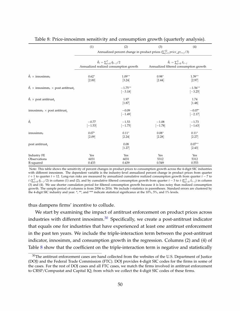
Table 8: Price-innosimm sensitivity and consumption growth (quarterly analysis).(1) (2) (3) (4)

Annualized percent change in product prices (∑12j=1 price_grt+j/3)

θt = ∑7j=0 ηt−j/2 θt = ∑3

j=0 xt−jAnnualized realized consumption growth Annualized filtered consumption growth

θt × innosimmt 0.62∗ 1.09∗∗ 0.98∗ 1.39∗∗

[2.00] [3.24] [2.44] [2.97]

θt × innosimmt × post antitrustt −1.75∗∗ −1.56∗∗

[−3.18] [−3.25]

θt × post antitrustt 1.97 1.74[1.87] [1.48]

innosimmt × post antitrustt −0.09 −0.07∗

[−1.49] [−2.17]

θt −0.77 −1.53 −1.08 −1.73[−1.53] [−1.75] [−1.78] [−1.63]

innosimmt 0.07∗ 0.11∗ 0.08∗ 0.11∗

[2.09] [2.24] [2.28] [2.27]

post antitrustt 0.08 0.07∗∗

[1.27] [2.43]

Industry FE Yes Yes Yes YesObservations 6031 6031 5312 5312R-squared 0.433 0.439 0.549 0.553

Note: This table shows the sensitivity of percent changes in product prices to consumption growth across the 4-digit SIC industrieswith different innosimm. The dependent variable is the industry-level annualized percent change in product prices from quartert + 1 to quarter t + 12. Long-run risks are measured by annualized cumulative realized consumption growth from quarter t− 7 tot (∑7

j=0 ηt−j/2) in column (1) and (2), and by cumulative filtered consumption growth from quarter t− 3 to t (∑3j=0 xt−j) in column

(3) and (4). We use shorter cumulation period for filtered consumption growth because it is less noisy than realized consumptiongrowth. The sample period of columns is from 2006 to 2016. We include t-statistics in parentheses. Standard errors are clustered bythe 4-digit SIC industry and year. *, **, and *** indicate statistical significance at the 10%, 5%, and 1% levels.

thus dampens firms’ incentive to collude.We start by examining the impact of antitrust enforcement on product prices across

industries with different innosimm.30 Specifically, we create a post-antitrust indicatorthat equals one for industries that have experienced at least one antitrust enforcementin the past ten years. We include the triple-interaction term between the post-antitrustindicator, innosimm, and consumption growth in the regression. Columns (2) and (4) ofTable 8 show that the coefficient on the triple-interaction term is negative and statistically

30The antitrust enforcement cases are hand collected from the websites of the U.S. Department of Justice(DOJ) and the Federal Trade Commission (FTC). DOJ provides 4-digit SIC codes for the firms in some ofthe cases. For the rest of DOJ cases and all FTC cases, we match the firms involved in antitrust enforcementto CRSP/Compustat and Capital IQ, from which we collect the 4-digit SIC codes of these firms.

50

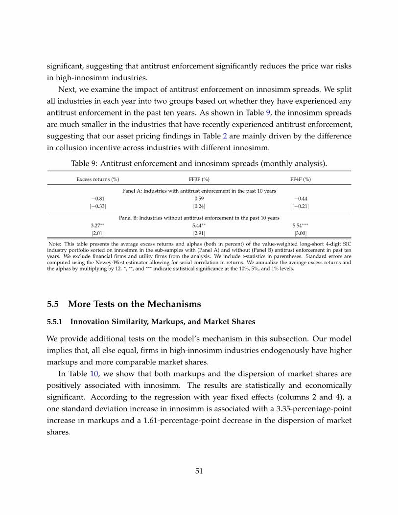
significant, suggesting that antitrust enforcement significantly reduces the price war risksin high-innosimm industries.

Next, we examine the impact of antitrust enforcement on innosimm spreads. We splitall industries in each year into two groups based on whether they have experienced anyantitrust enforcement in the past ten years. As shown in Table 9, the innosimm spreadsare much smaller in the industries that have recently experienced antitrust enforcement,suggesting that our asset pricing findings in Table 2 are mainly driven by the differencein collusion incentive across industries with different innosimm.

Table 9: Antitrust enforcement and innosimm spreads (monthly analysis).

Excess returns (%) FF3F (%) FF4F (%)

Panel A: Industries with antitrust enforcement in the past 10 years−0.81 0.59 −0.44[−0.33] [0.24] [−0.21]

Panel B: Industries without antitrust enforcement in the past 10 years3.27∗∗ 5.44∗∗ 5.54∗∗∗

[2.01] [2.91] [3.00]

Note: This table presents the average excess returns and alphas (both in percent) of the value-weighted long-short 4-digit SICindustry portfolio sorted on innosimm in the sub-samples with (Panel A) and without (Panel B) antitrust enforcement in past tenyears. We exclude financial firms and utility firms from the analysis. We include t-statistics in parentheses. Standard errors arecomputed using the Newey-West estimator allowing for serial correlation in returns. We annualize the average excess returns andthe alphas by multiplying by 12. *, **, and *** indicate statistical significance at the 10%, 5%, and 1% levels.

5.5 More Tests on the Mechanisms

5.5.1 Innovation Similarity, Markups, and Market Shares

We provide additional tests on the model’s mechanism in this subsection. Our modelimplies that, all else equal, firms in high-innosimm industries endogenously have highermarkups and more comparable market shares.

In Table 10, we show that both markups and the dispersion of market shares arepositively associated with innosimm. The results are statistically and economicallysignificant. According to the regression with year fixed effects (columns 2 and 4), aone standard deviation increase in innosimm is associated with a 3.35-percentage-pointincrease in markups and a 1.61-percentage-point decrease in the dispersion of marketshares.

51

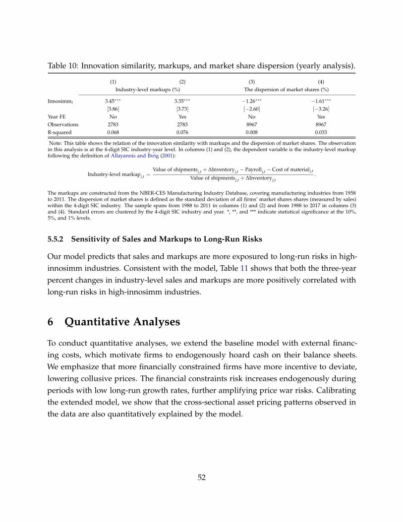
Table 10: Innovation similarity, markups, and market share dispersion (yearly analysis).

(1) (2) (3) (4)Industry-level markups (%) The dispersion of market shares (%)

Innosimmt 3.45∗∗∗ 3.35∗∗∗ −1.26∗∗∗ −1.61∗∗∗

[3.86] [3.73] [−2.60] [−3.26]Year FE No Yes No YesObservations 2783 2783 8967 8967R-squared 0.068 0.076 0.008 0.033

Note: This table shows the relation of the innovation similarity with markups and the dispersion of market shares. The observationin this analysis is at the 4-digit SIC industry-year level. In columns (1) and (2), the dependent variable is the industry-level markupfollowing the definition of Allayannis and Ihrig (2001):

Industry-level markupj,t =Value of shipmentsj,t + ∆Inventoryj,t − Payrollj,t −Cost of materialj,t

Value of shipmentsj,t + ∆Inventoryj,t.

The markups are constructed from the NBER-CES Manufacturing Industry Database, covering manufacturing industries from 1958to 2011. The dispersion of market shares is defined as the standard deviation of all firms’ market shares shares (measured by sales)within the 4-digit SIC industry. The sample spans from 1988 to 2011 in columns (1) and (2) and from 1988 to 2017 in columns (3)and (4). Standard errors are clustered by the 4-digit SIC industry and year. *, **, and *** indicate statistical significance at the 10%,5%, and 1% levels.

5.5.2 Sensitivity of Sales and Markups to Long-Run Risks

Our model predicts that sales and markups are more exposured to long-run risks in high-innosimm industries. Consistent with the model, Table 11 shows that both the three-yearpercent changes in industry-level sales and markups are more positively correlated withlong-run risks in high-innosimm industries.

6 Quantitative Analyses

To conduct quantitative analyses, we extend the baseline model with external financ-ing costs, which motivate firms to endogenously hoard cash on their balance sheets.We emphasize that more financially constrained firms have more incentive to deviate,lowering collusive prices. The financial constraints risk increases endogenously duringperiods with low long-run growth rates, further amplifying price war risks. Calibratingthe extended model, we show that the cross-sectional asset pricing patterns observed inthe data are also quantitatively explained by the model.

52

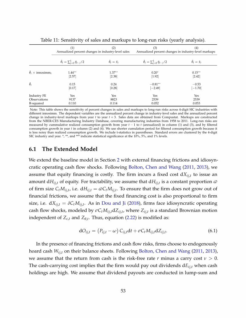
Table 11: Sensitivity of sales and markups to long-run risks (yearly analysis).(1) (2) (3) (4)

Annualized percent changes in industry-level sales Annualized percent changes in industry-level markups

θt = ∑1j=0 ηt−j/2 θt = xt θt = ∑1

j=0 ηt−j/2 θt = xt

θt × innosimmt 1.44∗∗ 1.37∗∗ 0.20∗ 0.15∗∗

[2.57] [2.38] [1.92] [2.42]

θt 0.15 0.24 −0.81∗∗ −0.53[0.17] [0.28] [−2.49] [−1.70]

Industry FE Yes Yes Yes YesObservations 9137 8823 2539 2539R-squared 0.110 0.114 0.052 0.053

Note: This table shows the sensitivity of percent changes in sales and markups to long-run risks across 4-digit SIC industries withdifferent innosimm. The dependent variables are the annualized percent change in industry-level sales and the annualized percentchange in industry-level markups from year t to year t + 3. Sales data are obtained from Compustat. Markups are constructedfrom the NBER-CES Manufacturing Industry Database, covering manufacturing industries from 1958 to 2011. Long-run risks aremeasured by cummulative realized consumption growth from year t − 1 to t (annualized) in column (1) and (3), and by filteredconsumption growth in year t in column (2) and (4). We use shorter cumulation period for filtered consumption growth because itis less noisy than realized consumption growth. We include t-statistics in parentheses. Standard errors are clustered by the 4-digitSIC industry and year. *, **, and *** indicate statistical significance at the 10%, 5%, and 1% levels.

6.1 The Extended Model

We extend the baseline model in Section 2 with external financing frictions and idiosyn-cratic operating cash flow shocks. Following Bolton, Chen and Wang (2011, 2013), weassume that equity financing is costly. The firm incurs a fixed cost dXij,t to issue anamount dHij,t of equity. For tractability, we assume that dHij,t is a constant proportion v

of firm size CtMij,t, i.e. dHij,t = vCtMij,t. To ensure that the firm does not grow out offinancial frictions, we assume that the fixed financing cost is also proportional to firmsize, i.e. dXij,t = δCtMij,t. As in Dou and Ji (2018), firms face idiosyncratic operatingcash flow shocks, modeled by σCtMij,tdZij,t, where Zij,t is a standard Brownian motionindependent of Zc,t and Zθ,t. Thus, equation (2.22) is modified as:

dOij,t =(

Pij,t −ω)

Cij,tdt + σCtMij,tdZij,t. (6.1)

In the presence of financing frictions and cash flow risks, firms choose to endogenouslyhoard cash Wij,t on their balance sheets. Following Bolton, Chen and Wang (2011, 2013),we assume that the return from cash is the risk-free rate r minus a carry cost ν > 0.The cash-carrying cost implies that the firm would pay out dividends dEij,t when cashholdings are high. We assume that dividend payouts are conducted in lump-sum and

53

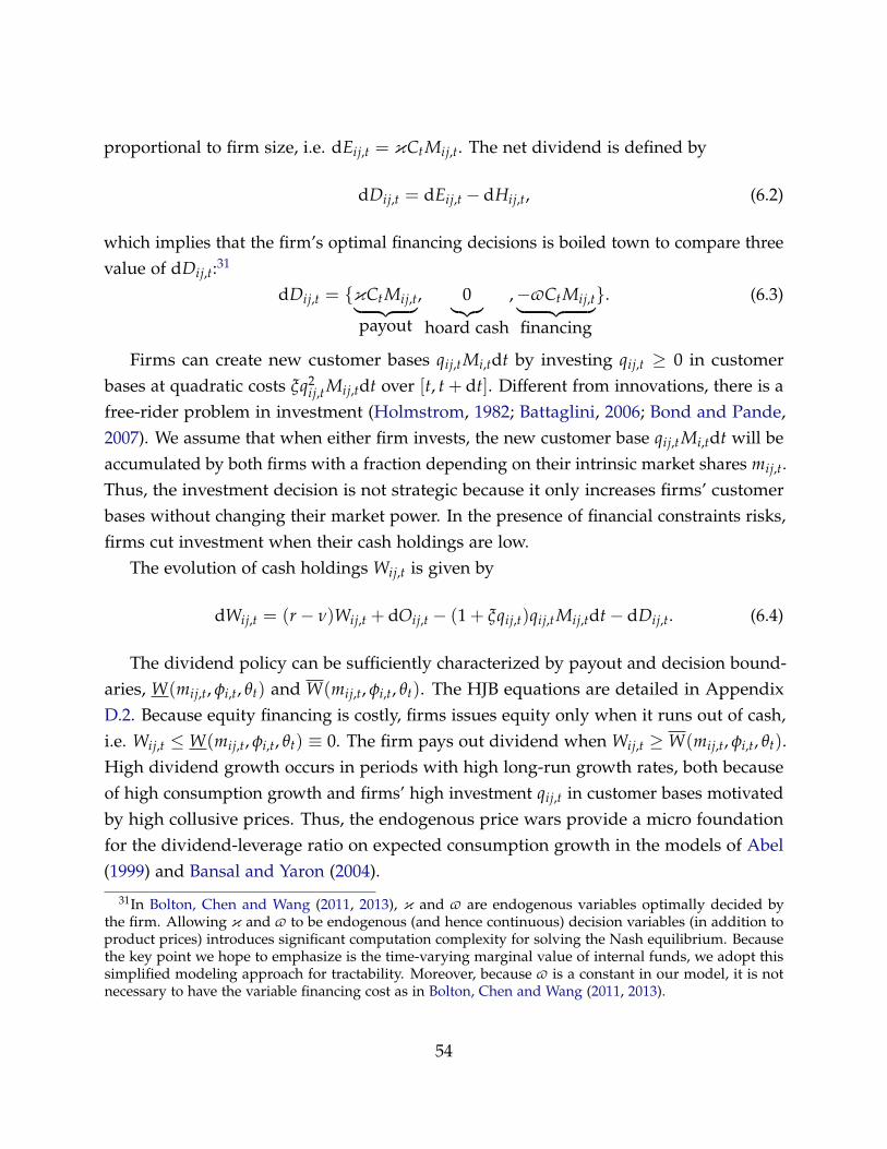
proportional to firm size, i.e. dEij,t = κCtMij,t. The net dividend is defined by

dDij,t = dEij,t − dHij,t, (6.2)

which implies that the firm’s optimal financing decisions is boiled town to compare threevalue of dDij,t:31

dDij,t = {κCtMij,t︸ ︷︷ ︸payout

, 0︸︷︷︸hoard cash

,−vCtMij,t︸ ︷︷ ︸financing

}. (6.3)

Firms can create new customer bases qij,tMi,tdt by investing qij,t ≥ 0 in customerbases at quadratic costs ξq2

ij,tMij,tdt over [t, t + dt]. Different from innovations, there is afree-rider problem in investment (Holmstrom, 1982; Battaglini, 2006; Bond and Pande,2007). We assume that when either firm invests, the new customer base qij,tMi,tdt will beaccumulated by both firms with a fraction depending on their intrinsic market shares mij,t.Thus, the investment decision is not strategic because it only increases firms’ customerbases without changing their market power. In the presence of financial constraints risks,firms cut investment when their cash holdings are low.

The evolution of cash holdings Wij,t is given by

dWij,t = (r− ν)Wij,t + dOij,t − (1 + ξqij,t)qij,tMij,tdt− dDij,t. (6.4)

The dividend policy can be sufficiently characterized by payout and decision bound-aries, W(mij,t, φi,t, θt) and W(mij,t, φi,t, θt). The HJB equations are detailed in AppendixD.2. Because equity financing is costly, firms issues equity only when it runs out of cash,i.e. Wij,t ≤W(mij,t, φi,t, θt) ≡ 0. The firm pays out dividend when Wij,t ≥W(mij,t, φi,t, θt).High dividend growth occurs in periods with high long-run growth rates, both becauseof high consumption growth and firms’ high investment qij,t in customer bases motivatedby high collusive prices. Thus, the endogenous price wars provide a micro foundationfor the dividend-leverage ratio on expected consumption growth in the models of Abel(1999) and Bansal and Yaron (2004).

31In Bolton, Chen and Wang (2011, 2013), κ and v are endogenous variables optimally decided bythe firm. Allowing κ and v to be endogenous (and hence continuous) decision variables (in addition toproduct prices) introduces significant computation complexity for solving the Nash equilibrium. Becausethe key point we hope to emphasize is the time-varying marginal value of internal funds, we adopt thissimplified modeling approach for tractability. Moreover, because v is a constant in our model, it is notnecessary to have the variable financing cost as in Bolton, Chen and Wang (2011, 2013).

54

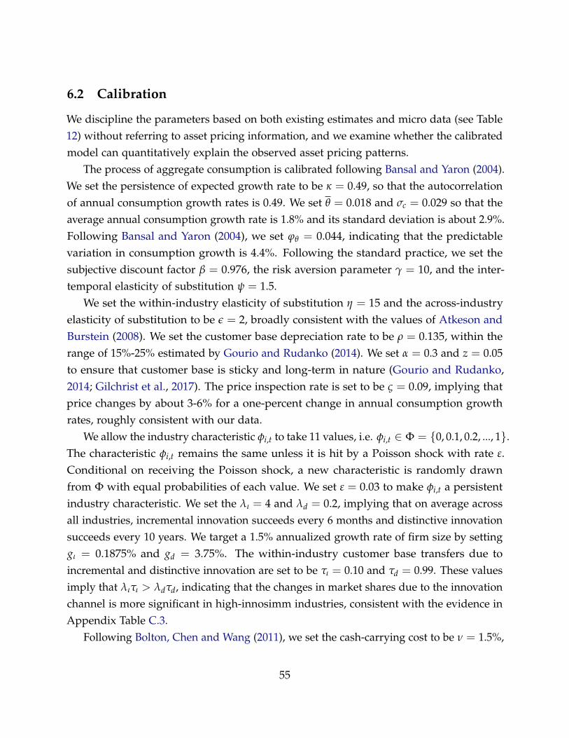
6.2 Calibration

We discipline the parameters based on both existing estimates and micro data (see Table12) without referring to asset pricing information, and we examine whether the calibratedmodel can quantitatively explain the observed asset pricing patterns.

The process of aggregate consumption is calibrated following Bansal and Yaron (2004).We set the persistence of expected growth rate to be κ = 0.49, so that the autocorrelationof annual consumption growth rates is 0.49. We set θ = 0.018 and σc = 0.029 so that theaverage annual consumption growth rate is 1.8% and its standard deviation is about 2.9%.Following Bansal and Yaron (2004), we set ϕθ = 0.044, indicating that the predictablevariation in consumption growth is 4.4%. Following the standard practice, we set thesubjective discount factor β = 0.976, the risk aversion parameter γ = 10, and the inter-temporal elasticity of substitution ψ = 1.5.

We set the within-industry elasticity of substitution η = 15 and the across-industryelasticity of substitution to be ε = 2, broadly consistent with the values of Atkeson andBurstein (2008). We set the customer base depreciation rate to be ρ = 0.135, within therange of 15%-25% estimated by Gourio and Rudanko (2014). We set α = 0.3 and z = 0.05to ensure that customer base is sticky and long-term in nature (Gourio and Rudanko,2014; Gilchrist et al., 2017). The price inspection rate is set to be ς = 0.09, implying thatprice changes by about 3-6% for a one-percent change in annual consumption growthrates, roughly consistent with our data.

We allow the industry characteristic φi,t to take 11 values, i.e. φi,t ∈ Φ = {0, 0.1, 0.2, ..., 1}.The characteristic φi,t remains the same unless it is hit by a Poisson shock with rate ε.Conditional on receiving the Poisson shock, a new characteristic is randomly drawnfrom Φ with equal probabilities of each value. We set ε = 0.03 to make φi,t a persistentindustry characteristic. We set the λι = 4 and λd = 0.2, implying that on average acrossall industries, incremental innovation succeeds every 6 months and distinctive innovationsucceeds every 10 years. We target a 1.5% annualized growth rate of firm size by settinggι = 0.1875% and gd = 3.75%. The within-industry customer base transfers due toincremental and distinctive innovation are set to be τι = 0.10 and τd = 0.99. These valuesimply that λιτι > λdτd, indicating that the changes in market shares due to the innovationchannel is more significant in high-innosimm industries, consistent with the evidence inAppendix Table C.3.

Following Bolton, Chen and Wang (2011), we set the cash-carrying cost to be ν = 1.5%,

55

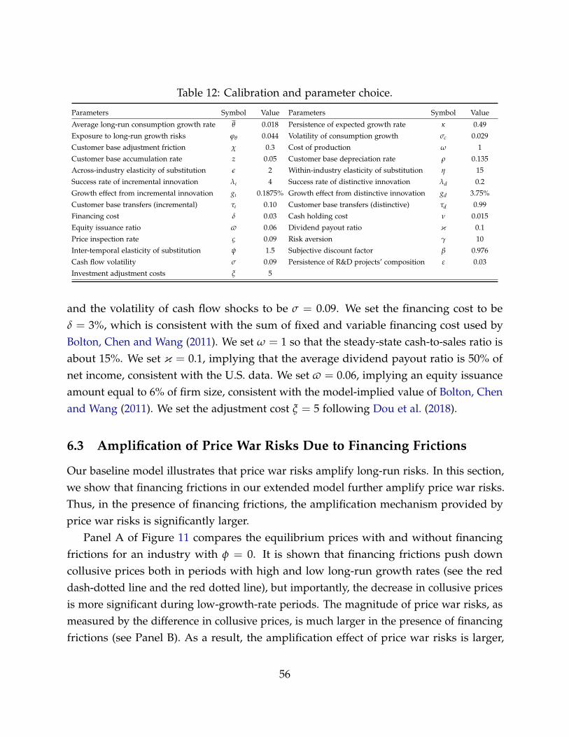
Table 12: Calibration and parameter choice.

Parameters Symbol Value Parameters Symbol Value

Average long-run consumption growth rate θ 0.018 Persistence of expected growth rate κ 0.49

Exposure to long-run growth risks ϕθ 0.044 Volatility of consumption growth σc 0.029

Customer base adjustment friction χ 0.3 Cost of production ω 1

Customer base accumulation rate z 0.05 Customer base depreciation rate ρ 0.135

Across-industry elasticity of substitution ε 2 Within-industry elasticity of substitution η 15

Success rate of incremental innovation λι 4 Success rate of distinctive innovation λd 0.2

Growth effect from incremental innovation gι 0.1875% Growth effect from distinctive innovation gd 3.75%

Customer base transfers (incremental) τι 0.10 Customer base transfers (distinctive) τd 0.99

Financing cost δ 0.03 Cash holding cost ν 0.015

Equity issuance ratio v 0.06 Dividend payout ratio κ 0.1

Price inspection rate ς 0.09 Risk aversion γ 10

Inter-temporal elasticity of substitution ψ 1.5 Subjective discount factor β 0.976

Cash flow volatility σ 0.09 Persistence of R&D projects’ composition ε 0.03

Investment adjustment costs ξ 5

and the volatility of cash flow shocks to be σ = 0.09. We set the financing cost to beδ = 3%, which is consistent with the sum of fixed and variable financing cost used byBolton, Chen and Wang (2011). We set ω = 1 so that the steady-state cash-to-sales ratio isabout 15%. We set κ = 0.1, implying that the average dividend payout ratio is 50% ofnet income, consistent with the U.S. data. We set v = 0.06, implying an equity issuanceamount equal to 6% of firm size, consistent with the model-implied value of Bolton, Chenand Wang (2011). We set the adjustment cost ξ = 5 following Dou et al. (2018).

6.3 Amplification of Price War Risks Due to Financing Frictions

Our baseline model illustrates that price war risks amplify long-run risks. In this section,we show that financing frictions in our extended model further amplify price war risks.Thus, in the presence of financing frictions, the amplification mechanism provided byprice war risks is significantly larger.

Panel A of Figure 11 compares the equilibrium prices with and without financingfrictions for an industry with φ = 0. It is shown that financing frictions push downcollusive prices both in periods with high and low long-run growth rates (see the reddash-dotted line and the red dotted line), but importantly, the decrease in collusive pricesis more significant during low-growth-rate periods. The magnitude of price war risks, asmeasured by the difference in collusive prices, is much larger in the presence of financingfrictions (see Panel B). As a result, the amplification effect of price war risks is larger,

56

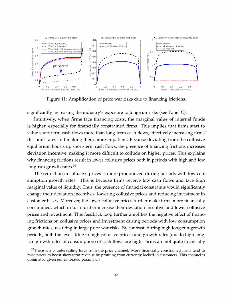
0 0.2 0.4 0.6 0.8 1

1.2

1.4

1.6

1.8

2

2.2

0 0.2 0.4 0.6 0.8 1

0

0.1

0.2

0.3

0.4

0.5

0.6

0.7

0.8

0 0.2 0.4 0.6 0.8 1

1.5

2

2.5

3

Figure 11: Amplification of price war risks due to financing frictions.

significantly increasing the industry’s exposure to long-run risks (see Panel C).Intuitively, when firms face financing costs, the marginal value of internal funds

is higher, especially for financially constrained firms. This implies that firms start tovalue short-term cash flows more than long-term cash flows, effectively increasing firms’discount rates and making them more impatient. Because deviating from the collusiveequilibrium boosts up short-term cash flows, the presence of financing frictions increasesdeviation incentive, making it more difficult to collude on higher prices. This explainswhy financing frictions result in lower collusive prices both in periods with high and lowlong-run growth rates.32

The reduction in collusive prices is more pronounced during periods with low con-sumption growth rates. This is because firms receive low cash flows and face highmarginal value of liquidity. Thus, the presence of financial constraints would significantlychange their deviation incentives, lowering collusive prices and reducing investment incustomer bases. Moreover, the lower collusive prices further make firms more financiallyconstrained, which in turn further increase their deviation incentive and lower collusiveprices and investment. This feedback loop further amplifies the negative effect of financ-ing frictions on collusive prices and investment during periods with low consumptiongrowth rates, resulting in large price war risks. By contrast, during high long-run-growthperiods, both the levels (due to high collusive prices) and growth rates (due to high long-run growth rates of consumption) of cash flows are high. Firms are not quite financially

32There is a countervailing force from the price channel. More financially constrained firms tend toraise prices to boost short-term revenue by profiting from currently locked-in customers. This channel isdominated given our calibrated parameters.

57

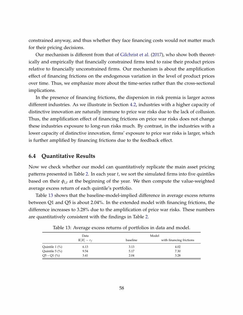
constrained anyway, and thus whether they face financing costs would not matter muchfor their pricing decisions.

Our mechanism is different from that of Gilchrist et al. (2017), who show both theoret-ically and empirically that financially constrained firms tend to raise their product pricesrelative to financially unconstrained firms. Our mechanism is about the amplificationeffect of financing frictions on the endogenous variation in the level of product pricesover time. Thus, we emphasize more about the time-series rather than the cross-sectionalimplications.

In the presence of financing frictions, the dispersion in risk premia is larger acrossdifferent industries. As we illustrate in Section 4.2, industries with a higher capacity ofdistinctive innovation are naturally immune to price war risks due to the lack of collusion.Thus, the amplification effect of financing frictions on price war risks does not changethese industries exposure to long-run risks much. By contrast, in the industries with alower capacity of distinctive innovation, firms’ exposure to price war risks is larger, whichis further amplified by financing frictions due to the feedback effect.

6.4 Quantitative Results

Now we check whether our model can quantitatively replicate the main asset pricingpatterns presented in Table 2. In each year t, we sort the simulated firms into five quintilesbased on their φi,t at the beginning of the year. We then compute the value-weightedaverage excess return of each quintile’s portfolio.

Table 13 shows that the baseline-model-implied difference in average excess returnsbetween Q1 and Q5 is about 2.04%. In the extended model with financing frictions, thedifference increases to 3.28% due to the amplification of price war risks. These numbersare quantitatively consistent with the findings in Table 2.

Table 13: Average excess returns of portfolios in data and model.

Data ModelE[R] − r f baseline with financing frictions

Quintile 1 (%) 6.13 3.13 4.02Quintile 5 (%) 9.54 5.17 7.30Q5 – Q1 (%) 3.41 2.04 3.28

58

7 Conclusion

In this paper, we explore the the implication of price war risks. We develop a general-equilibrium asset pricing model incorporating dynamic supergames of price competitionamong firms. In our model, price wars can arise endogenously from declines in long-runconsumption growth, since firms become effectively more impatient for cash flows andtheir incentives to undercut prices become stronger.

Our model implies that financial frictions amplify price war risks, which in turnlargely amplify long-run risks and generate cross-sectional implications on stock returns.The exposure to price war risks reflect predictable and persistent heterogeneous industrycharacteristics. Firms in industries with more frequent distinctive innovation are moreimmune to price war risks due to the higher likelihood of creative destruction and marketdisruption. Exploring detailed patent and product price data, we found evidence for theexistence of price war risks. Moreover, that endogenous price war risks are priced in thecross section.

ReferencesAaker, David A. 2012. Building Strong Brands. Simon and Schuster.

Abel, Andrew B. 1990. “Asset Prices under Habit Formation and Catching Up with the Joneses.” AmericanEconomic Review, 80(2): 38–42.

Abel, Andrew B. 1999. “Risk premia and term premia in general equilibrium.” Journal of Monetary Economics,43(1): 3–33.

Abreu, Dilip, David Pearce, and Ennio Stacchetti. 1986. “ Optimal cartel equilibria with imperfect moni-toring.” Journal of Economic Theory, 39(1): 251–269.

Abreu, Dilip, David Pearce, and Ennio Stacchetti. 1990. “Toward a Theory of Discounted Repeated Gameswith Imperfect Monitoring.” Econometrica, 58(5): 1041–1063.

Aguerrevere, Felipe L. 2009. “Real Options, Product Market Competition, and Asset Returns.” Journal ofFinance, 64(2): 957–983.

Aguiar, Mark, and Erik Hurst. 2007. “Life-cycle prices and production.” American Economic Review,97(5): 1533–1559.

Ai, Hengjie. 2010. “Information quality and long-run risk: Asset pricing implications.” Journal of Finance,65(4): 1333–1367.

Ai, Hengjie, and Dana Kiku. 2013. “Growth to Value: Option Exercise and the Cross Section of EquityReturns.” Journal of Financial Economics, 107(2): 325–349.

59

Ai, Hengjie, Kai Li, Jun Li, and Christian Schlag. 2018. “The Collateralizability Premium.” Workingpapers.

Ai, Hengjie, Mariano Massimiliano Croce, and Kai Li. 2013. “Toward a Quantitative General EquilibriumAsset Pricing Model with Intangible Capital.” Review of Financial Studies, 26(2): 491–530.

Ali, Ashiq, Sandy Klasa, and Eric Yeung. 2008. “The limitations of industry concentration measures con-structed with Compustat data: Implications for finance research.” Review of Financial Studies, 22(10): 3839–3871.

Allayannis, George, and Jane Ihrig. 2001. “Exposure and markups.” Review of Financial Studies, 14(3): 805–835.

Allen, Jeffrey W, and Gordon M Phillips. 2000. “Corporate equity ownership, strategic alliances, andproduct market relationships.” Journal of Finance, 55(6): 2791–2815.

Andrei, Daniel, and Bruce I. Carlin. 2018. “The Risk of Schumpeterian Competition.” Working Paper,UCLA Anderson School of Management.

Argente, David, Munseob Lee, and Sara Moreira. 2018. “Innovation and product reallocation in the greatrecession.” Journal of Monetary Economics, 93: 1–20.

Athey, Susan, Kyle Bagwell, and Chris Sanchirico. 2004. “Collusion and Price Rigidity.” Review of EconomicStudies, 71(2): 317–349.

Atkeson, Andrew, and Ariel Burstein. 2008. “Pricing-to-Market, Trade Costs, and International RelativePrices.” American Economic Review, 98(5): 1998–2031.

Autor, David, David Dorn, Lawrence F. Katz, Christina Patterson, and John Van Reenen. 2017. “TheFall of the Labor Share and the Rise of Superstar Firms.” Centre for Economic Performance, LSE CEPDiscussion Papers.

Bagwell, Kyle, and Robert Staiger. 1997. “Collusion Over the Business Cycle.” RAND Journal of Economics,28(1): 82–106.

Bansal, Ravi, and Amir Yaron. 2004. “Risks for the Long Run: A Potential Resolution of Asset PricingPuzzles.” Journal of Finance, 59(4): 1481–1509.

Bansal, Ravi, Dana Kiku, and Amir Yaron. 2012. “An Empirical Evaluation of the Long-Run Risks Modelfor Asset Prices.” Critical Finance Review, 1(1): 183–221.

Bansal, Ravi, Dana Kiku, and Amir Yaron. 2016. “Risks for the long run: Estimation with time aggregation.”Journal of Monetary Economics, 82: 52–69.

Bansal, Ravi, Robert Dittmar, and Dana Kiku. 2009. “Cointegration and Consumption Risks in AssetReturns.” Review of Financial Studies, 22(3): 1343–1375.

Bansal, Ravi, Robert F. Dittmar, and Christian T. Lundblad. 2005. “Consumption, Dividends, and theCross Section of Equity Returns.” Journal of Finance, 60(4): 1639–1672.

Battaglini, Marco. 2006. “Joint production in teams.” Journal of Economic Theory, 130: 138–167.

Belo, Frederico, and Xiaoji Lin. 2012. “The Inventory Growth Spread.” Review of Financial Studies, 25(1): 278–313.

60

Belo, Frederico, Xiaoji Lin, and Fan Yang. 2018. “External Equity Financing Shocks, Financial Flows, andAsset Prices.” Review of Financial Studies, forthcoming.

Belo, Frederico, Xiaoji Lin, and Maria Ana Vitorino. 2014. “Brand Capital and Firm Value.” Review ofEconomic Dynamics, 17(1): 150–169.

Belo, Frederico, Xiaoji Lin, and Santiago Bazdresch. 2014. “Labor Hiring, Investment, and Stock ReturnPredictability in the Cross Section.” Journal of Political Economy, 122(1): 129–177.

Bergin, James, and W Bentley MacLeod. 1993. “Continuous Time Repeated Games.” International EconomicReview, 34(1): 21–37.

Berk, Jonathan B., Richard C. Green, and Vasant Naik. 1999. “Optimal Investment, Growth Options, andSecurity Returns.” Journal of Finance, 54(5): 1553–1607.

Biais, Bruno, David Martimort, and Jean-Charles Rochet. 2000. “Competing Mechanisms in a CommonValue Environment.” Econometrica, 68(4): 799–838.

Bloom, Nicholas, Mark Schankerman, and John Van Reenen. 2013. “Identifying technology spilloversand product market rivalry.” Econometrica, 81(4): 1347–1393.

Bolton, Patrick, Hui Chen, and Neng Wang. 2011. “A Unified Theory of Tobin’s q, Corporate Investment,Financing, and Risk Management.” Journal of Finance, 66(5): 1545–1578.

Bolton, Patrick, Hui Chen, and Neng Wang. 2013. “Market timing, investment, and risk management.”Journal of Financial Economics, 109(1): 40–62.

Bond, Philip, and Arvind Krishnamurthy. 2004. “Regulating Exclusion from Financial Markets.” Reviewof Financial Studies, 71(3): 681–707.

Bond, Philip, and Rohini Pande. 2007. “Coordinating development: Can income-based incentive schemeseliminate Pareto inferior equilibria?” Journal of Development Economics, 83(2): 368–391.

Brock, William A, and Jose A Scheinkman. 1985. “Price setting supergames with capacity constraints.”The Review of Economic Studies, 52(3): 371–382.

Broda, Christian, and David E Weinstein. 2010. “Product creation and destruction: Evidence and priceimplications.” American Economic Review, 100(3): 691–723.

Bustamante, Maria Cecilia. 2015. “Strategic investment and industry risk dynamics.” Review of FinancialStudies, 28(2): 297–341.

Bustamante, M. Cecilia, and Andres Donangelo. 2017. “Product Market Competition and Industry Re-turns.” Review of Financial Studies, 30(12): 4216–4266.

Campbell, John, Jens Hilscher, and Jan Szilagyi. 2008. “In Search of Distress Risk.” Journal of Finance,63(6): 2899–2939.

Campbell, John Y, and Robert J Shiller. 1988. “The dividend-price ratio and expectations of futuredividends and discount factors.” Review of Financial Studies, 1(3): 195–228.

Carhart, Mark M. 1997. “On Persistence in Mutual Fund Performance.” Journal of Finance, 52(1): 57–82.

61

Carlin, Bruce I. 2009. “Strategic price complexity in retail financial markets.” Journal of Financial Economics,91(3): 278 – 287.

Carlson, Murray, Engelbert J. Dockner, Adlai Fisher, and Ron Giammarino. 2014. “Leaders, Followers,and Risk Dynamics in Industry Equilibrium.” Journal of Financial and Quantitative Analysis, 49(2): 321–349.

Chan, Yeung Lewis, and Leonid Kogan. 2002. “Catching Up with the Joneses: Heterogeneous Preferencesand the Dynamics of Asset Prices.” Journal of Political Economy, 110(6): 1255–1285.

Chen, Hui. 2010. “Macroeconomic Conditions and the Puzzles of Credit Spreads and Capital Structure.”The Journal of Finance, 65(6): 2171–2212.

Chevalier, Judith A, and David S Scharfstein. 1996. “Capital-Market Imperfections and CountercyclicalMarkups: Theory and Evidence.” American Economic Review, 86(4): 703–25.

Christensen, Clayton. 1997. The innovator’s dilemma: when new technologies cause great firms to fail. HarvardBusiness Review Press.

Christie, William, and Paul H Schultz. 1994. “Why Do NASDAQ Market Makers Avoid Odd-EighthQuotes?” Journal of Finance, 49(5): 1813–40.

Cochrane, John H. 1991. “ Production-Based Asset Pricing and the Link between Stock Returns andEconomic Fluctuations.” Journal of Finance, 46(1): 209–237.

Constantinides, George M., and Anisha Ghosh. 2011. “Asset Pricing Tests with Long-run Risks in Con-sumption Growth.” Review of Asset Pricing Studies, 1(1): 96–136.

Corhay, Alexandre. 2017. “Industry competition, credit spreads, and levered equity returns.” University ofToronto Working Papers.

Corhay, Alexandre, Howard Kung, and Lukas Schmid. 2017. “Competition, markups, and predictablereturns.” Working Papers.

Croce, Mariano Massimiliano. 2014. “Long-run productivity risk: A new hope for production-based assetpricing?” Journal of Monetary Economics, 66(C): 13–31.

D’Acunto, Francesco, Ryan Liu, Carolin Pflueger, and Michael Weber. 2018. “Flexible prices and leverage.”Journal of Financial Economics, 129(1): 46–68.

Dittmar, Robert F, and Christian T Lundblad. 2017. “Firm characteristics, consumption risk, and firm-levelrisk exposures.” Journal of Financial Economics, 125(2): 326–343.

Donangelo, Andres. 2014. “Labor Mobility: Implications for Asset Pricing.” Journal of Finance, 68(3): 1321–1346.

Dou, Winston. 2017. “Embrace or Fear Uncertainty: Growth Options, Limited Risk Sharing, and AssetPrices.” University of Pennsylvania.

Dou, Winston Wei, and Yan Ji. 2018. “External Financing and Customer Capital: A Financial Theory ofMarkups.” Working Papers.

Dou, Winston, Yan Ji, David Reibstein, and Wei Wu. 2018. “Customer Capital, Financial Constraints, andStock Returns.” Working Papers.

62

Duffie, Darrell, and Larry G. Epstein. 1992a. “Asset Pricing with Stochastic Differential Utility.” Review ofFinancial Studies, 5(3): 411–36.

Duffie, Darrell, and Larry G. Epstein. 1992b. “Stochastic Differential Utility.” Econometrica, 60(2): 353–94.

Edmans, Alex, Itay Goldstein, and Wei Jiang. 2015. “Feedback Effects, Asymmetric Trading, and theLimits to Arbitrage.” American Economic Review, 105(12): 3766–3797.

Eisfeldt, Andrea L., and Dimitris Papanikolaou. 2013. “Organization Capital and the Cross-Section ofExpected Returns.” Journal of Finance, 68(4): 1365–1406.

Eisfeldt, Andrea L., and Tyler Muir. 2016. “Aggregate External Financing and Savings Waves.” Journal ofMonetary Economics, 84: 116–133.

Epstein, Larry G., and Stanley E. Zin. 1989. “Substitution, Risk Aversion, and the Temporal Behavior ofConsumption and Asset Returns: A Theoretical Framework.” Econometrica, 57(4): 937–69.

Ericson, Richard, and Ariel Pakes. 1995. “Markov-Perfect Industry Dynamics: A Framework for EmpiricalWork.” Review of Economic Studies, 62(1): 53–82.

Fama, Eugene F., and Kenneth R. French. 1993. “Common Risk Factors in the Returns on Stocks andBonds.” Journal of Financial Economics, 33(1): 3–56.

Fershtman, Chaim, and Ariel Pakes. 2000. “A Dynamic Oligopoly with Collusion and Price Wars.” RANDJournal of Economics, 31(2): 207–236.

Fitzgerald, Tristan, Benjamin Balsmeier, Lee Fleming, and Gustavo Manso. 2017. “Innovation searchstrategy and predictable returns: A bias for novelty.” Working Paper, University of California at Berkeley.

Fudenberg, Drew, and Jean Tirole. 1991. Game Theory. The MIT Press.

Garlappi, Lorenzo, and Hong Yan. 2011. “Financial Distress and the Cross-Section of Equity Returns.”Journal of Finance, 66(3): 789–822.

Gârleanu, Nicolae, Leonid Kogan, and Stavros Panageas. 2012. “Displacement risk and asset returns.”Journal of Financial Economics, 105(3): 491 – 510.

Gârleanu, Nicolae, Stavros Panageas, and Jianfeng Yu. 2012. “Technological Growth and Asset Pricing.”Journal of Finance, 67(4): 1265–1292.

Gerzema, John, and Edward Lebar. 2008. The Brand Bubble: The Looming Crisis in Brand Value and How toAvoid It. Jossey-Bass.

Gilchrist, Simon, Jae Sim, Raphael Schoenle, and Egon Zakrajsek. 2017. “Inflation Dynamics During theFinancial Crisis.” American Economic Review, 107(3): 785–823.

Gomes, Joao, and Lukas Schmid. 2018. “Equilibrium Asset Pricing with Leverage and Default.” Journal ofFinance, forthcoming.

Gomes, Joao F. 2001. “Financing Investment.” American Economic Review, 91(5): 1263–1285.

Gomes, Joao F., and Lukas Schmid. 2010. “Levered Returns.” Journal of Finance, 65(2): 467–494.

63

Gomes, Joao, Leonid Kogan, and Lu Zhang. 2003. “Equilibrium Cross Section of Returns.” Journal ofPolitical Economy, 111(4): 693–732.

Gourio, Francois, and Leena Rudanko. 2014. “Customer Capital.” Review of Economic Studies, 81(3): 1102–1136.

Green, Edward J, and Robert H Porter. 1984. “Noncooperative Collusion under Imperfect Price Informa-tion.” Econometrica, 52(1): 87–100.

Hackbarth, Dirk, and Bart Taub. 2018. “Does the Potential to Merge Reduce Competition?” WorkingPaper.

Hackbarth, Dirk, and Jianjun Miao. 2012. “The dynamics of mergers and acquisitions in oligopolisticindustries.” Journal of Economic Dynamics and Control, 36(4): 585–609.

Hall, Bronwyn H, Adam B Jaffe, and Manuel Trajtenberg. 2001. “The NBER patent citation data file:Lessons, insights and methodological tools.” National Bureau of Economic Research.

Haltiwanger, John, and Joseph E. Harrington. 1991. “The Impact of Cyclical Demand Movements onCollusive Behavior.” RAND Journal of Economics, 22(1): 89–106.

Hansen, Lars Peter, John C Heaton, and Nan Li. 2005. “Intangible risk.” In Measuring Capital in the NewEconomy. 111–152. University of Chicago Press.

Hansen, Lars Peter, John C Heaton, and Nan Li. 2008. “Consumption strikes back? Measuring long-runrisk.” Journal of Political Economy, 116(2): 260–302.

He, Zhiguo, and Wei Xiong. 2012. “Rollover Risk and Credit Risk.” Journal of Finance, 67(2): 391–430.

Hirshleifer, David A., Po-Hsuan Hsu, and Dongmei Li. 2017. “Innovative Originality, Profitability, andStock Returns.” Review of Financial Studies, forthcoming.

Hirshleifer, David, Po-Hsuan Hsu, and Dongmei Li. 2013. “Innovative efficiency and stock returns.”Journal of Financial Economics, 107(3): 632–654.

Hoberg, Gerard, and Gordon Phillips. 2010. “Product market synergies and competition in mergers andacquisitions: A text-based analysis.” Review of Financial Studies, 23(10): 3773–3811.

Hoberg, Gerard, and Gordon Phillips. 2016. “Text-based network industries and endogenous productdifferentiation.” Journal of Political Economy, 124(5): 1423–1465.

Hoberg, Gerard, Gordon Phillips, and Nagpurnanand Prabhala. 2014. “Product market threats, payouts,and financial flexibility.” Journal of Finance, 69(1): 293–324.

Holmstrom, Bengt. 1982. “Moral Hazard in Teams.” Bell Journal of Economics, 13(2): 324–340.

Hottman, Colin J, Stephen J Redding, and David E Weinstein. 2016. “Quantifying the sources of firmheterogeneity.” Quarterly Journal of Economics, 131(3): 1291–1364.

Hou, Kewei, and David T. Robinson. 2006. “Industry Concentration and Average Stock Returns.” Journalof Finance, 61(4): 1927–1956.

Jaffe, Adam B. 1986. “Technological Opportunity and Spillovers of R & D: Evidence from Firms’ Patents,Profits, and Market Value.” The American Economic Review, 76(5): 984–1001.

64

Jaravel, Xavier. 2018. “The unequal gains from product innovations: Evidence from the us retail sector.”Quarterly Journal of Economics, forthcoming.

Kandel, Shmuel, and Robert F. Stambaugh. 1991. “Asset returns and intertemporal preferences.” Journalof Monetary Economics, 27(1): 39–71.

Keller, Kevin Lane. 2008. Strategic Brand Management: Building, Measuring, and Managing Brand Equity.Pearson Education.

Kelly, Bryan, Dimitris Papanikolaou, Amit Seru, and Matt Taddy. 2018. “Measuring technological inno-vation over the long run.” Working Paper.

Klemperer, Paul. 1995. “Competition when Consumers have Switching Costs: An Overview with Applica-tions to Industrial Organization, Macroeconomics, and International Trade.” Review of Economic Studies,62(4): 515–539.

Kogan, Leonid, and Dimitris Papanikolaou. 2013. “Firm Characteristics and Stock Returns: The Role ofInvestment-Specific Shocks.” Review of Financial Studies, 26: 2718–2759.

Kogan, Leonid, and Dimitris Papanikolaou. 2014. “Growth Opportunities, Technology Shocks, and AssetPrices.” Journal of Finance, 69(2): 675–718.

Kogan, Leonid, Dimitris Papanikolaou, Amit Seru, and Noah Stoffman. 2017. “Technological innovation,resource allocation, and growth.” Quarterly Journal of Economics, 132(2): 665–712.

Kogan, Leonid, Dimitris Papanikolaou, and Noah Stoffman. 2018. “Winners and Losers: Creative De-struction and the Stock Market.” Working Papers.

Kogan, Leonid, Dimitris Papanikolaou, Lawrence Schmidt, and Jae Song. 2018. “Technological Innova-tion and the Distribution of Labor Income Growth.” Working Papers.

Koijen, Ralph S.J., Hanno Lustig, and Stijn Van Nieuwerburgh. 2017. “The cross-section and time seriesof stock and bond returns.” Journal of Monetary Economics, 88: 50–69.

Kovenock, Dan, and Gordon M Phillips. 1997. “Capital structure and product market behavior: Anexamination of plant exit and investment decisions.” Review of Financial Studies, 10(3): 767–803.

Kozak, Serhiy, Stefan Nagel, and Shrihari Santosh. 2017. “Shrinking the Cross Section.” National Bureauof Economic Research, Inc NBER Working Papers 24070.

Kreps, David M., and Evan L. Porteus. 1978. “Temporal Resolution of Uncertainty and Dynamic ChoiceTheory.” Econometrica, 46(1): 185–200.

Kumar, Praveen, and Dongmei Li. 2016. “Capital investment, innovative capacity, and stock returns.”Journal of Finance, 71(5): 2059–2094.

Kung, Howard, and Lukas Schmid. 2015. “Innovation, Growth, and Asset Prices.” Journal of Finance,70(3): 1001–1037.

Lerner, Josh, and Amit Seru. 2017. “The use and misuse of patent data: Issues for corporate finance andbeyond.” National Bureau of Economic Research.

Li, Dongmei. 2011. “Financial Constraints, R&D Investment, and Stock Returns.” Review of Financial Studies,24(9): 2974–3007.

65

Liu, Hong, and Yajun Wang. 2018. “Asset Pricing Implications of Short-Sale Constraints in ImperfectlyCompetitive Markets.” Management Science, 1–18.

Livdan, Dmitry, Horacio Sapriza, and Lu Zhang. 2009. “Financially Constrained Stock Returns.” Journalof Finance, 64(4): 1827–1862.

Loecker, Jan De, and Jan Eeckhout. 2017. “The Rise of Market Power and the Macroeconomic Implications.”National Bureau of Economic Research, Inc NBER Working Papers.

Longstaff, Francis A., and Monika Piazzesi. 2004. “Corporate earnings and the equity premium.” Journalof Financial Economics, 74(3): 401–421.

Loualiche, Erik. 2016. “Asset Pricing with Entry and Imperfect Competition.” Working Papers.

Lovett, Mitchell, Renana Peres, and Ron Shachar. 2014. “A Data Set of Brands and Their Characteristics.”Marketing Science, 33(4): 609–617.

Lucas, Robert E, Jr. 1978. “Asset Prices in an Exchange Economy.” Econometrica, 46(6): 1429–1445.

Malloy, Christopher J., Tobias J. Moskowitz, and Annette Vissing-Jørgensen. 2009. “Long-Run Stock-holder Consumption Risk and Asset Returns.” Journal of Finance, 64(6): 2427–2479.

Manso, Gustavo. 2011. “Motivating innovation.” Journal of Finance, 66(5): 1823–1860.

Martin, Ian. 2013. “The Lucas Orchard.” Econometrica, 81(1): 55–111.

Maskin, Eric, and Jean Tirole. 2001. “Markov Perfect Equilibrium: I. Observable Actions.” Journal ofEconomic Theory, 100(2): 191 – 219.

Menzly, Lior, Tano Santos, and Pietro Veronesi. 2004. “Understanding Predictability.” Journal of PoliticalEconomy, 112(1): 1–47.

Mizik, Natalie, and Robert Jacobson. 2008. “The Financial Value Impact of Perceptual Brand Attributes.”Journal of Marketing Research, 45(1): 15–32.

Nagel, Stefan. 2005. “Short Sales, Institutional Investors and the Cross-Section of Stock Returns.” Journal ofFinancial Economics, 78(2): 277–309.

Nagel, Stefan. 2013. “Empirical Cross-Sectional Asset Pricing.” Annual Review of Financial Economics,5(1): 167–199.

Opp, Marcus M., Christine A. Parlour, and Johan Walden. 2014. “Markup cycles, dynamic misallocation,and amplification.” Journal of Economic Theory, 154(C): 126–161.

Pakes, Ariel, and Paul McGuire. 1994. “Computing Markov-Perfect Nash Equilibria: Numerical Implica-tions of a Dynamic Differentiated Product Model.” RAND Journal of Economics, 25(4): 555–589.

Pastor, Lubos, and Robert F. Stambaugh. 2003. “Liquidity Risk and Expected Stock Returns.” Journal ofPolitical Economy, 111(3): 642–685.

Phillips, Gordon M. 1995. “Increased debt and industry product markets an empirical analysis.” Journal ofFinancial Economics, 37(2): 189–238.

66

Ravn, Morten, Stephanie Schmitt-Grohe, and Martin Uribe. 2006. “Deep Habits.” Review of EconomicStudies, 73(1): 195–218.

Riddick, Leigh A., and Toni M. Whited. 2009. “The Corporate Propensity to Save.” Journal of Finance,64(4): 1729–1766.

Rotemberg, Julio J, and Garth Saloner. 1986. “A Supergame-Theoretic Model of Price Wars during Booms.”American Economic Review, 76(3): 390–407.

Rotemberg, Julio J., and Michael Woodford. 1991. “Markups and the Business Cycle.” In NBER Macroeco-nomics Annual 1991, Volume 6. NBER Chapters, 63–140. National Bureau of Economic Research, Inc.

Rouwenhorst, K. Geert. 1995. “Asset pricing implications of equilibrium business cycle models.” In In:Cooley, T.F. (Ed.), Frontiers of Business Cycle Research. 294–330. Princeton University Press, Princeton, NJ.

Santos, Tano, and Pietro Veronesi. 2006. “Habit formation, the cross section of stock returns and thecash-flow risk puzzle.” Review of Financial Studies, 19(1): 1–44.

Santos, Tano, and Pietro Veronesi. 2010. “Habit formation, the cross section of stock returns and thecash-flow risk puzzle.” Journal of Financial Economics, 98(2): 385–413.

Schorfheide, Frank, Dongho Song, and Amir Yaron. 2018. “Identifying long-run risks: A bayesian mixed-frequency approach.” Econometrica, forthcoming.

Staiger, Robert W., and Frank A. Wolak. 1992. “Collusive Pricing with Capacity Constraints in the Presenceof Demand Uncertainty.” RAND Journal of Economics, 23(2): 203–220.

Stigler, George J. 1964. “A Theory of Oligopoly.” Journal of Political Economy, 72(1): 44–61.

Tauchen, George. 1986. “Finite state markov-chain approximations to univariate and vector autoregressions.”Economics Letters, 20: 177–181.

Tavassoli, Nader T., Alina Sorescu, and Rajesh Chandy. 2014. “Employee-Based Brand Equity: Why Firmswith Strong Brands Pay Their Executives Less.” Journal of Marketing Research, 51(6): 676–690.

Tirole, Jean. 1988. The Theory of Industrial Organization. Vol. 1 of MIT Press Books, The MIT Press.

Tsai, Jerry, and Jessica A. Wachter. 2016. “Rare booms and disasters in a multi-sector endowment economy.”Review of Financial Studies, 29(5): 1377–1408.

Wachter, Jessica. 2013. “Can Time-Varying Risk of Rare Disasters Explain Aggregate Stock Market Volatil-ity?” Journal of Finance, 68(3): 987–1035.

Weber, Michael. 2015. “Nominal Rigidities and Asset Pricing.” Working Paper.

Weil, Philippe. 1990. “Nonexpected Utility in Macroeconomics.” The Quarterly Journal of Economics,105(1): 29–42.

Weiser, Alan, and Sergio E. Zarantonello. 1988. “A Note on Piecewise Linear and Multilinear TableInterpolation in Many Dimensions.” Mathematics of Computation, 50(181): 189–196.

Xiong, Wei, and Hongjun Yan. 2010. “Heterogeneous Expectations and Bond Markets.” Review of FinancialStudies, 23(4): 1433–1466.

67

Appendix

A Headline Quotes for Price Wars and Stock ReturnsWe cite a few recent media headlines on how price wars can depress firms’ stock returns.

• “Best Buy Co. shares plunged 11% Tuesday, after the electronics chain warned investors about pricewar fears.” – The Wall Street Journal on November 20th of 2013.

• “Target shares dive as it shifts to cut-price strategy.” – Financial Times on February 28th of 2017.

• “Price war eats into the profits of pharmaceutical wholesalers and manufacturers alike and erasesbillions of dollars of the market value in recent days” – The Wall Street Journal on August 5th of 2017.

• “Airline stocks plunge on price war fears.” – Financial Times on January 24th of 2018.

• “Investors Purge Infinera Stock on Price War Concerns, Ignore Q1 Results.” – SDxCentral on May10th of 2018.

• “A fierce price war between consumer goods giants hit Unilever shares hard.” – The Wall StreetJournal on July 19th of 2018.

• “Coffee price war takes jolt out of Dunkin’ results.” – Financial Times on September 27th of 2018.

B Data

B.1 Industry Concentration RatioWe use the U.S. Census concentration ratio data from 1987, 1992, 1997, 2002, 2007, and 2012 to computethe time-series maximal and mean revenue shares for the top 4 firms (CR4) and top 8 firms (CR8) in each4-digit SIC industry. The concentration ratios are at the 6-digit NAICS level after 1997. We follow Ali, Klasaand Yeung (2008) and convert the ratios to 4-digit SIC levels. Figure B.1 plots the histogram of the maxCR4 (Panel A1), max CR8 (Panel B1), mean CR4 (Panel A2), and mean CR8 (Panel B2) in all 4-digit SICindustries. Red vertical lines represent the cross-sectional mean values.

B.2 Match PatentView with CRSP/Compustat/Capital IQIn this Appendix, we detail the matching procedure for the data from PatentView, CRSP/Compustat, andCapital IQ.33 We first drop patent assignees that are classified as individuals and government agencies byPatentView, because these assignees are not associated with any particular industry. We then clean assigneenames in PatentView and firm names in CRSP/Compustat and Capital IQ following the approach of Hall,Jaffe and Trajtenberg (2001). To elaborate, we remove punctuations and clean special characters. We then

33The PatentView data are available at http://www.patentsview.org/download/.

68

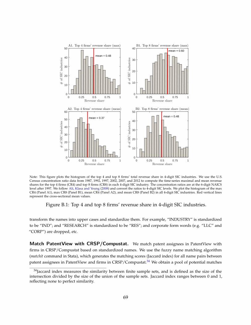
Revenue share0 0.25 0.5 0.75 1

#of

SIC

industries

0

10

20

30

40

50

mean = 0.48

A1. Top 4 firms’ revenue share (max)

Revenue share0 0.25 0.5 0.75 1

#of

SIC

industries

0

10

20

30

40mean = 0.60

B1. Top 8 firms’ revenue share (max)

Revenue share0 0.25 0.5 0.75 1

#of

SIC

industries

0

10

20

30

40

50

60

mean = 0.37

A2. Top 4 firms’ revenue share (mean)

Revenue share0 0.25 0.5 0.75 1

#of

SIC

industries

0

10

20

30

40

50

mean = 0.48

B2. Top 8 firms’ revenue share (mean)

Note: This figure plots the histogram of the top 4 and top 8 firms’ total revenue share in 4-digit SIC industries. We use the U.S.Census concentration ratio data from 1987, 1992, 1997, 2002, 2007, and 2012 to compute the time-series maximal and mean revenueshares for the top 4 firms (CR4) and top 8 firms (CR8) in each 4-digit SIC industry. The concentration ratios are at the 6-digit NAICSlevel after 1997. We follow Ali, Klasa and Yeung (2008) and convert the ratios to 4-digit SIC levels. We plot the histogram of the maxCR4 (Panel A1), max CR8 (Panel B1), mean CR4 (Panel A2), and mean CR8 (Panel B2) in all 4-digit SIC industries. Red vertical linesrepresent the cross-sectional mean values.

Figure B.1: Top 4 and top 8 firms’ revenue share in 4-digit SIC industries.

transform the names into upper cases and standardize them. For example, “INDUSTRY” is standardizedto be “IND”; and “RESEARCH” is standardized to be “RES”; and corporate form words (e.g. “LLC” and“CORP”) are dropped, etc.

Match PatentView with CRSP/Compustat. We match patent assignees in PatentView withfirms in CRSP/Compustat based on standardized names. We use the fuzzy name matching algorithm(matchit command in Stata), which generates the matching scores (Jaccard index) for all name pairs betweenpatent assignees in PatentView and firms in CRSP/Compustat.34 We obtain a pool of potential matches

34Jaccard index measures the similarity between finite sample sets, and is defined as the size of theintersection divided by the size of the union of the sample sets. Jaccard index ranges between 0 and 1,reflecting none to perfect similarity.

69

based on two criteria: (1) we require the matching score to be higher than 0.6; (2) we require the first threeletters of patent assignees to be the same as those of firms in CRSP/Compustat.35 We then go through allpotential matches to manually identify exact matches.36

As pointed out by Lerner and Seru (2017), one major challenge for linking patent data to CRSP/Compustatis that some patent assignees are subsidiaries of firms in CRSP/Compustat. For these assignees, we cannotdirectly match them with CRSP/Compustat based on firm names. To deal with this challenge, the NBERpatent data (Hall, Jaffe and Trajtenberg, 2001) use the 1989 edition of the Who Owns Whom directory (nowknown as the D&B WorldBase R©- Who Owns Whom) to match subsidiaries to parent companies. Koganet al. (2017) purged the matches identified by the NBER patent data, and extended the matching betweenpatent data and CRSP/Compustat to 2010. For those patent assignees who are subsidiaries of firms inCRSP/Compustat, we augment our matches by incorporating the data of Kogan et al. (2017) for patentsgranted before 2010. For patents granted after 2010, we use the subsidiary-parent link table from the 2017snapshot of the Orbis data to match subsidiaries in PatentView to their parent firms in CRSP/Compustat.

Match PatentView with Capital IQ. We match the remaining patent assignees in PatentViewwith firms in Capital IQ following the same matching procedure. To keep the workload manageable, wedrop firms in Capital IQ whose assets are worth less than $100 million (in 2017 dollars). Because we focuson the U.S. product market, we also drop foreign firms whose asset values are below the 90th percentile ofthe asset value distribution among firms in the CRSP/Compustat sample in each year, respectively. This isbecause small foreign firms are less likely to have a material impact on the competition environment of theU.S. product market. We match PatentView to Capital IQ directly using the information on subsidiariesprovided by Capital IQ.

B.3 Construct Dividend GrowthWe follow previous studies (see e.g. Campbell and Shiller, 1988; Bansal, Dittmar and Lundblad, 2005;Hansen, Heaton and Li, 2005, 2008; Bansal, Kiku and Yaron, 2016) to contrust dividend growth rates ofportfolios.

Denote V0t as the market value of all firms in a given portfolio. Denote the value of this portfolio atdate t + 1 to be Vt+1. The aggregate dividends for data t + 1 for this portfolio is Dt+1. The total return onthe portfolio between t and t + 1 is:

Rt+1 =Vt+1 + Dt+1

V0t= ht+1 + dt+1. (B.1)

where ht+1 is the price appreciation, which represents the ratio of the value at time t + 1 to time t (i.e.,Vt+1V0t

), while dt+1 is the dividend yield, which represents the total dividends paid by at time t + 1 divied by

35These two matching criteria are sufficiently conservative to ensure that exact matches are included inthe pool of potential matches. For example, among all the exact matches in the first quarter of 2016, 98% ofthem satisfy the two matching criteria and are included in our pool of potential matches.

36We rely on assignee names in PatentView and firm names in CRSP/Compustat to identify matches. Inaddition, we use location information in both datasets to facilitate the matching process.

70

portfolio value at time t (i.e., Dt+1V0t

).Holding the portfolio composition constant (i.e., no exits and entries), the real dividend growth rate is:

Dt+1/PCEt+1

Dt/PCEt=

dt+1V0t

dtV0(t−1)

PCEt

PCEt+1=

dt+1ht

dt

PCEt

PCEt+1=

(Rt+1 − ht+1)ht

Rt − ht

PCEt

PCEt+1, (B.2)

where PCE is the personal consumption expenditure deflator from the U.S. BEA.Because stocks move in and out of portfolios, we account for the entries and exits following the literature

(see e.g. Hansen, Heaton and Li, 2005, 2008; Bansal, Kiku and Yaron, 2016) by adding an adjustment term.Specifically, the real dividend growth rate for a portfolio is:

Vt

V0t

Dt+1/PCEt+1

Dt/PCEt, (B.3)

where Vt is exit value of the portfolio at time t (i.e., the time t market value of firms in the portfolio formedat time t− 1), and V0t is the market value of firms in the new position we initiate at time t. Plug equationB.2 into B.3, the real dividend growth rate for a portfolio is:

Vt

V0t

Dt+1/PCEt+1

Dt/PCEt=

Vt

V0t

(Rt+1 − ht+1)ht

Rt − ht

PCEt

PCEt+1. (B.4)

We calculate portfolio Rt and ht by computing the value-weighted RET and RETX (both from CRSP)across firms within the portfolio. Since share repurchases are prevelant in our sample period, we followBansal, Dittmar and Lundblad (2005) and adjust the capital gain series for a given firm as following:

RETX∗t+1 = RETXt+1 min[(

nt+1

nt

), 1]

, (B.5)

where nt is the number of shares after adjusting for splits, stock dividends, etc using the CRSP shareadjustment factor.

B.4 Match Nielsen with CRSP/Compustat/Capital IQWe follow previous studies (e.g. Hottman, Redding and Weinstein, 2016; Argente, Lee and Moreira, 2018;Jaravel, 2018) to find the companies that own the products in the Nielsen data using the product-firmlink table in the “GS1 US Data Hub | Company” data, which is provided by GS1 – the official source ofUPCs in the U.S.37 We match 95.3% of the products in the Nielsen data with firms in the GS1 data. Ourmatching rate is the same as those reported by Argente, Lee and Moreira (2018) and Jaravel (2018). Wefurther match the companies in the GS1 data to CRSP/Compustat and Capital IQ to find their SIC industrycodes. The matching procedures are the same as patent matching. Our merged data cover products in 472SIC industries.

37The “GS1 US Data Hub | Company” data provide the company names, company addresses, and theUPC prefixes owned by the companies. More information about the “GS1 US Data Hub | Company” isavailable at: https://www.gs1us.org/tools/gs1-us-data-hub/company.

71

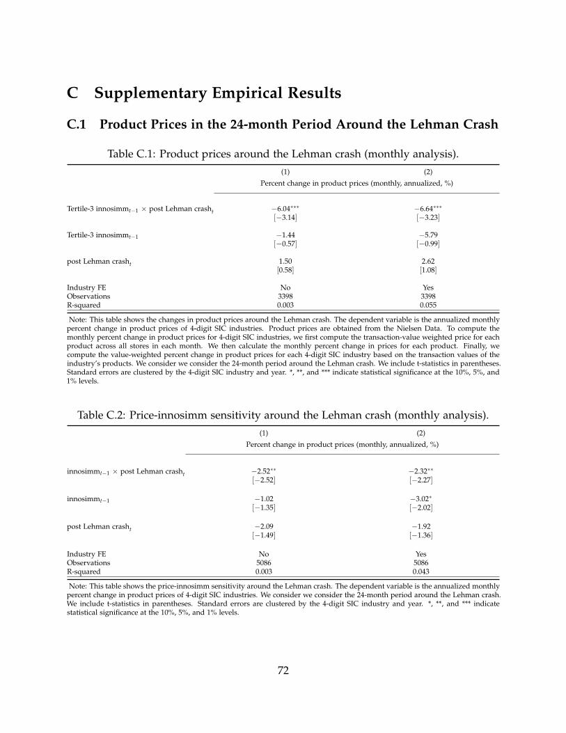
C Supplementary Empirical Results

C.1 Product Prices in the 24-month Period Around the Lehman Crash

Table C.1: Product prices around the Lehman crash (monthly analysis).(1) (2)

Percent change in product prices (monthly, annualized, %)

Tertile-3 innosimmt−1 × post Lehman crasht −6.04∗∗∗ −6.64∗∗∗

[−3.14] [−3.23]

Tertile-3 innosimmt−1 −1.44 −5.79[−0.57] [−0.99]

post Lehman crasht 1.50 2.62[0.58] [1.08]

Industry FE No YesObservations 3398 3398R-squared 0.003 0.055

Note: This table shows the changes in product prices around the Lehman crash. The dependent variable is the annualized monthlypercent change in product prices of 4-digit SIC industries. Product prices are obtained from the Nielsen Data. To compute themonthly percent change in product prices for 4-digit SIC industries, we first compute the transaction-value weighted price for eachproduct across all stores in each month. We then calculate the monthly percent change in prices for each product. Finally, wecompute the value-weighted percent change in product prices for each 4-digit SIC industry based on the transaction values of theindustry’s products. We consider we consider the 24-month period around the Lehman crash. We include t-statistics in parentheses.Standard errors are clustered by the 4-digit SIC industry and year. *, **, and *** indicate statistical significance at the 10%, 5%, and1% levels.

Table C.2: Price-innosimm sensitivity around the Lehman crash (monthly analysis).(1) (2)

Percent change in product prices (monthly, annualized, %)

innosimmt−1 × post Lehman crasht −2.52∗∗ −2.32∗∗

[−2.52] [−2.27]

innosimmt−1 −1.02 −3.02∗

[−1.35] [−2.02]

post Lehman crasht −2.09 −1.92[−1.49] [−1.36]

Industry FE No YesObservations 5086 5086R-squared 0.003 0.043

Note: This table shows the price-innosimm sensitivity around the Lehman crash. The dependent variable is the annualized monthlypercent change in product prices of 4-digit SIC industries. We consider we consider the 24-month period around the Lehman crash.We include t-statistics in parentheses. Standard errors are clustered by the 4-digit SIC industry and year. *, **, and *** indicatestatistical significance at the 10%, 5%, and 1% levels.

72

C.2 The Sensitivity of Market Shares to Innovative OutputsIn this Appendix, we examine the relation between innovation similarity and the sensitivity of marketshares to innovative outputs. Specifically, we regress the changes in firms’ market shares on the firm’s owninnovative outputs, peers’ innovative outputs, lagged innosimm, the interaction term between innosimmand the firm’s own innovative outputs, and the interaction term between innosimm and peers’ innovativeoutputs. Table C.3 shows that the coefficient of the interaction term between innosimm and the firm’s owninnovative outputs is significantly positive, while the coefficient of the interaction term between innosimmand peers’ innovative outputs is significantly negative. These findings suggest that in high-innosimmindustries, firms obtain more market shares from their own innovation, but also lose more market sharesfrom their peers’ innovation. These results are economically significant. Consider two firms, one in anindustry with the mean value of innosimm and the other is in an industry whose innosimm is one standarddeviation above the mean. According to the regression specification with year fixed effect (column 4 ofTable C.3), the latter firm’s market share increases by 8.3 percentage points more in two years in response toa one standard deviation increase in the firm’s own innovative outputs. Moreover, the latter firm’s marketshare decreases by 4.2 percentage points more in two years in response to a one standard deviation increasein peers’ innovative outputs.

D Numerical AlgorithmIn this section, we detail the numerical algorithm that solves the model. To give an overview, our algorithmproceeds in the following steps:

(1). We solve for the non-collusive equilibrium. This requires us to solve the Markov-Perfect equilibriumof the dynamic game played by two firms. The simultaneous-move dynamic game requires us tosolve the intersection of the two firms’ best response (i.e. optimal price) functions, which themselvesare optimal solutions to coupled PDEs.

(2). We solve for the collusive equilibrium using the value functions in the non-collusive equilibrium aspunishment values. Because we are interested in the highest collusive prices with binding incentive-compatibility constraints, this requires us to solve a high-dimensional fixed-points problem. We thususe an iteration method inspired by and to solve the problem (Abreu, Pearce and Stacchetti, 1986,1990; Ericson and Pakes, 1995; Fershtman and Pakes, 2000).

(3). After solving the baseline model, we solve the extended model with endogenous cash holdings byrepeating steps (1) and (2). The extended model is more challenging because it involves solvingPDEs with free boundaries (due to endogenous payout boundaries). We employ the piecewisemultilinear interpolation method of Weiser and Zarantonello (1988) to obtain accurate interpolantsin a 3-dimensional space.

Note that standard methods for solving PDEs with free boundaries (e.g. finite difference or finiteelement) can easily lead to non-convergence of value functions. To mitigate such problems and obtainaccurate solutions, we solve the continuous-time game using a discrete-time dynamic programming method.

73

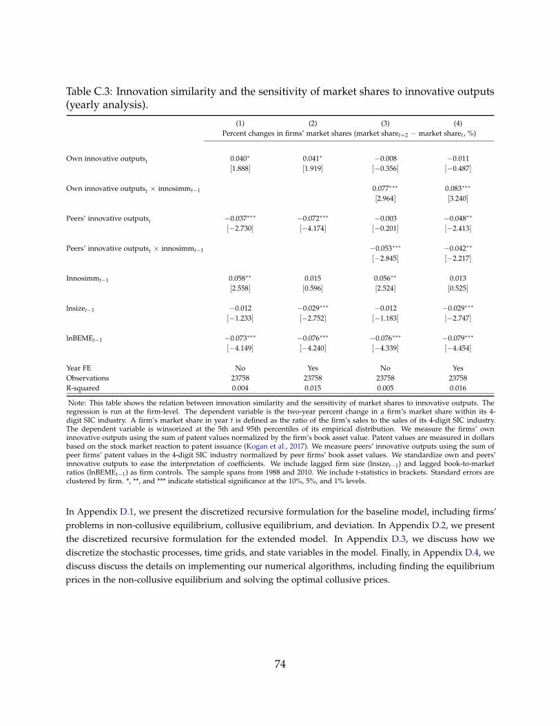
Table C.3: Innovation similarity and the sensitivity of market shares to innovative outputs(yearly analysis).

(1) (2) (3) (4)Percent changes in firms’ market shares (market sharet+2 − market sharet, %)

Own innovative outputst 0.040∗ 0.041∗ −0.008 −0.011[1.888] [1.919] [−0.356] [−0.487]

Own innovative outputst × innosimmt−1 0.077∗∗∗ 0.083∗∗∗

[2.964] [3.240]

Peers’ innovative outputst −0.037∗∗∗ −0.072∗∗∗ −0.003 −0.048∗∗

[−2.730] [−4.174] [−0.201] [−2.413]

Peers’ innovative outputst × innosimmt−1 −0.053∗∗∗ −0.042∗∗

[−2.845] [−2.217]

Innosimmt−1 0.058∗∗ 0.015 0.056∗∗ 0.013[2.558] [0.596] [2.524] [0.525]

lnsizet−1 −0.012 −0.029∗∗∗ −0.012 −0.029∗∗∗

[−1.233] [−2.752] [−1.183] [−2.747]

lnBEMEt−1 −0.073∗∗∗ −0.076∗∗∗ −0.076∗∗∗ −0.079∗∗∗

[−4.149] [−4.240] [−4.339] [−4.454]

Year FE No Yes No YesObservations 23758 23758 23758 23758R-squared 0.004 0.015 0.005 0.016

Note: This table shows the relation between innovation similarity and the sensitivity of market shares to innovative outputs. Theregression is run at the firm-level. The dependent variable is the two-year percent change in a firm’s market share within its 4-digit SIC industry. A firm’s market share in year t is defined as the ratio of the firm’s sales to the sales of its 4-digit SIC industry.The dependent variable is winsorized at the 5th and 95th percentiles of its empirical distribution. We measure the firms’ owninnovative outputs using the sum of patent values normalized by the firm’s book asset value. Patent values are measured in dollarsbased on the stock market reaction to patent issuance (Kogan et al., 2017). We measure peers’ innovative outputs using the sum ofpeer firms’ patent values in the 4-digit SIC industry normalized by peer firms’ book asset values. We standardize own and peers’innovative outputs to ease the interpretation of coefficients. We include lagged firm size (lnsizet−1) and lagged book-to-marketratios (lnBEMEt−1) as firm controls. The sample spans from 1988 and 2010. We include t-statistics in brackets. Standard errors areclustered by firm. *, **, and *** indicate statistical significance at the 10%, 5%, and 1% levels.

In Appendix D.1, we present the discretized recursive formulation for the baseline model, including firms’problems in non-collusive equilibrium, collusive equilibrium, and deviation. In Appendix D.2, we presentthe discretized recursive formulation for the extended model. In Appendix D.3, we discuss how wediscretize the stochastic processes, time grids, and state variables in the model. Finally, in Appendix D.4, wediscuss discuss the details on implementing our numerical algorithms, including finding the equilibriumprices in the non-collusive equilibrium and solving the optimal collusive prices.

74

D.1 The Baseline ModelBecause firm 1 and firm 2 are symmetric, one firm’s value and policy functions are obtained directly giventhe other firm’s value and policy functions. In this section, we illustrate firm 1’s problem in our baselinemodel. We first illustrate the non-collusive equilibrium and then we illustrate the collusive equilibrium.

D.1.1 Non-Collusive Equilibrium

Below, we present the recursive formulation for the firm’s value in the non-collusive equilibrium. Then weexploit linearity to simplify the problem and present the recursive formulation for the normalized firmvalue. Finally, we present the conditions that determine the non-collusive (Nash) equilibrium.

Recursive Formulation for The Non-Collusive Firm Value. The industry’s state is charac-terized by five state variables, firm 1’s customer base Mi1,t, firm 2’s customer base Mi2,t, the industry’sR&D characteristic φi,t, the aggregate consumption Ct, and the long-run growth rate θt. Denote the valuefunctions in the non-collusive equilibrium as VN

ij (Mi1,t, Mi2,t, φi,t, Ct, θt) for j = 1, 2.To characterize the equilibrium value functions, it is more convenient to introduce two off-equilibrium

value functions. Let VNij (Mi1,t, Mi2,t, φi,t, Ct, θt; Pik,t) be firm j(= 1, 2)’s value when its peer firm k’s price is

set at any (off-equilibrium) value Pik,t.Firm 1 solves the following problem:

VNi1 (Mi1,t, Mi2,t, φi,t, Ct, θt; Pi2,t) =max

Pi1,t(Pi1,t −ω)

(Pi1,t

Pi,t

)−η

P−εi,t Ct Mi1,t∆t

+ Et

[Λt+∆t

ΛtVN

i1 (Mi1,t+∆t, Mi2,t+∆t, φi,t+∆t, Ct+∆t, θt+∆t)

], (D.1)

subject to the evolution of state variables, including:The evolution of the customer base is

Mij,t+∆t =Mij,t +

[z(Cij,t

Ct

)α

M1−αij,t − ρMij,t

]∆t + Mik,t(τι∆I ι

ij,t + τd∆Idij,t) + Mi,t(gι∆I ι

ij,t + gd∆Idij,t)

−Mij,t(τι∆I ιik,t + τd∆Id

ik,t), for j = 1, 2 (D.2)

where firm-level demand is given by

Cij,t =

(Pij,t

Pi,t

)−η

P−εi,t Ct Mij,t, for j = 1, 2 (D.3)

and the industry’s price index is given by

Pi,t =

(Mi1,t

Mi,tP1−η

i1,t +Mi2,t

Mi,tP1−η

i2,t

) 11−η

. (D.4)

75

The evolution of aggregate consumption Ct is

Ct+∆t = (1 + θt∆t + σ∆Zc,t)Ct, (D.5)

The industry’s R&D characteristic φi,t and the long-run growth rate θt evolves according to the discreteMarkov chain specified in Appendix D.3.

Recursive Formulation for The (Normalized) Non-Collusive Firm Value. Exploiting thelinearity, we normalize the firm’s value by Mi,tCt. Firm 1’s intrinsic market share is mi1,t = Mi1,t/Mi,t; firm2’s intrinsic market share is mi2,t = Mi2,t/Mi,t = 1−mi1,t. Define

vNij (mi1,t, φi,t, θt) =

VNij (Mi1,t, Mi2,t, φi,t, Ct, θt)

Mi,tCt(D.6)

vNij (mi1,t, φi,t, θt; Pik,t) =

VNij (Mi1,t, Mi2,t, φi,t, Ct, θt; Pik,t)

Mi,tCt(D.7)

Firm 1 solves the following normalized problem:

vNi1(mi1,t, φi,t, θt; Pi2,t) =max

Pi1,t(Pi1,t −ω)

(Pi1,t

Pi,t

)−η

P−εi,t mi1,t∆t

+ Et

[Λt+∆t

Λt

Mi,t+∆t

Mi,t(1 + θt∆t + σ∆Zc,t)vN

i1(mi1,t+∆t, φi,t+∆t, θt+∆t)

], (D.8)

subject to the evolution of state variables, including:The evolution of firm 1’s intrinsic market share is

mi1,t+∆tMi,t+∆t

Mi,t=mi1,t +

[z(

Pi1,t

Pi,t

)−ηα

P−εαi,t − ρ

]mi1,t∆t + (1−mi1,t)(τι∆I ι

i1,t + τd∆Idi1,t) + (gι∆I ι

i1,t + gd∆Idi1,t)

−mi1,t(τι∆I ιi2,t + τd∆Id

i2,t), (D.9)

where the industry’s price index is given by

Pi,t =[mi1,tP

1−ηi1,t + (1−mi1,t)P1−η

i2,t

] 11−η . (D.10)

The evolution of the industry’s customer base is

Mi,t+∆t

Mi,t=1 +

[z(

Pi1,t

Pi,t

)−ηα

P−εαi,t − ρ

]mi1,t∆t +

[z(

Pi2,t

Pi,t

)−ηα

P−εαi,t − ρ

](1−mi1,t)∆t

+ gι∆I ιi1,t + gd∆Id

i1,t + gι∆I ιi2,t + gd∆Id

i2,t. (D.11)

The industry’s R&D characteristic φi,t and the long-run growth rate θt evolve according to the discreteMarkov chain specified in Appendix D.3.

76

Non-Collusive (Nash) Equilibrium. Denote the equilibrium price functions as PNij (mi1,t, φi,t, θt) and

the off-equilibrium price functions as PNij (mi1,t, φi,t, θt; Pik,t). Exploiting the symmetry between firm 1 and

firm 2, we can obtain firm 2’s off-equilibrium value and policy functions as

vNi1(mi1,t, φi,t, θt; Pi2,t) =vN

i2(1−mi1,t, φi,t, θt; Pi1,t), (D.12)

PNi1 (mi1,t, φi,t, θt; Pi2,t) =PN

i2 (1−mi1,t, φi,t, θt; Pi1,t). (D.13)

Given j = 1, 2’s price Pij, firm k optimally sets the price Pik. The non-collusive (Nash) equilibrium isderived from the fixed point—each firm’s price is optimal given the other firm’s optimal price:

PNi1 (mi1,t, φi,t, θt) =PN

i1 (mi1,t, φi,t, θt; PNi2 (mi1,t, φi,t, θt)), (D.14)

PNi2 (mi1,t, φi,t, θt) =PN

i2 (mi1,t, φi,t, θt; PNi1 (mi1,t, φi,t, θt)). (D.15)

The equilibrium value functions are given by

vNi1(mi1,t, φi,t, θt) =vN

i1(mi1,t, φi,t, θt; PNi2 (mi1,t, φi,t, θt)), (D.16)

vNi2(mi1,t, φi,t, θt) =vN

i2(mi1,t, φi,t, θt; PNi1 (mi1,t, φi,t, θt)). (D.17)

After solving the equilibrium value and policy functions above, we can verify that the followingconditions are satisfied due to symmetry,

vNi1(mi1,t, φi,t, θt) =vN

i2(1−mi1,t, φi,t, θt), (D.18)

PNi1 (mi1,t, φi,t, θt) =PN

i2 (1−mi1,t, φi,t, θt). (D.19)

D.1.2 Collusive Equilibrium

Below, we present the recursive formulation for the firm’s value in the collusive equilibrium. Then wepresent the recursive formulation for the firm’s value when the firm deviates from the collusive equilibrium.Finally, we present the incentive compatibility constraints and the conditions that determine the optimalcollusive prices.

Recursive Formulation for The Collusive Firm Value. In the collusive equilibrium, we canstill exploit the linearity property and solve firms’ values as a function of intrinsic market shares. Specif-ically, denote vC

ij(mi1,t, φi,t, θt; PCij ) as firm j’s value in the collusive equilibrium with collusive prices

PCij (mi1,t, φi,t, θt). Note that because the two firms in the same industry are symmetric, the collusive prices

satisfy PCi1(mi1,t, φi,t, θt) = PC

i2(1−mi1,t, φi,t, θt).

77

Firm 1 solves the following normalized problem:

vCi1(mi1,t, φi,t, θt; PC

ij ) =(

PCi1(mi1,t, φi,t, θt)−ω

)( PCi1(mi1,t, φi,t, θt)

Pi,t

)−η

P−εi,t mij,t∆t

+ Et

[Λt+∆t

Λt

Mi,t+∆t

Mi,t(1 + θt∆t + σ∆Zc,t)vC

i1(mi1,t+∆t, φi,t+∆t, θt+∆t; PCij )

], (D.20)

subject to the evolution of state variables, including:The evolution of firm 1’s intrinsic market share is

mi1,t+∆tMi,t+∆t

Mi,t=mi1,t +

z

(PC

i1(mi1,t, φi,t, θt)

Pi,t

)−ηα

P−εαi,t − ρ

mi1,t∆t + (1−mi1,t)(τι∆I ιi1,t + τd∆Id

i1,t)

+ (gι∆I ιi1,t + gd∆Id

i1,t)−mi1,t(τι∆I ιi2,t + τd∆Id

i2,t), (D.21)

where the industry’s price index is given by

Pi,t =[mi1,t PC

i1(mi1,t, φi,t, θt)1−η + (1−mi1,t)PC

i2(mi1,t, φi,t, θt)1−η] 1

1−η . (D.22)

The evolution of the industry’s customer base is

Mi,t+∆t

Mi,t=1 +

z

(PC

i1(mi1,t, φi,t, θt)

Pi,t

)−ηα

P−εαi,t − ρ

mi1,t∆t +

z

(PC

i2(mi1,t, φi,t, θt)

Pi,t

)−ηα

P−εαi,t − ρ

(1−mi1,t)∆t

+ gι∆I ιi1,t + gd∆Id

i1,t + gι∆I ιi2,t + gd∆Id

i2,t. (D.23)

The industry’s R&D characteristic φi,t and the long-run growth rate θt evolve according to the discreteMarkov chain specified in Appendix D.3.

Recursive Formulation for The Deviation Value. The deviation value is obtained by assumingthat firm j optimally sets its price conditional on firm k following the collusive pricing rule PC

ik(mi1,t, φi,t, θt).We exploit the linearity property and solve firms’ deviation values as a function of intrinsic market shares.Denote vD

ij (mi1,t, φi,t, θt; PCij ) as firm j’s deviation value.

Firm 1 solves the following normalized problem:

vDi1(mi1,t, φi,t, θt; PC

ij ) = maxPi1,t

(Pi1,t −ω)

(Pi1,t

Pi,t

)−η

P−εi,t mij,t∆t

+ Et

[Λt+∆t

Λt

Mi,t+∆t

Mi,t(1 + θt∆t + σ∆Zc,t)

[(1− ς∆t)vD

i1(mi1,t+∆t, φi,t+∆t, θt+∆t; PCij ) + ς∆tvN

i1(mi1,t+∆t, φi,t+∆t, θt+∆t)]]

,

(D.24)

subject to the evolution of state variables, including:

78

The evolution of firm 1’s intrinsic market share is

mi1,t+∆tMi,t+∆t

Mi,t=mi1,t +

[z(

Pi1,t

Pi,t

)−ηα

P−εαi,t − ρ

]mi1,t∆t + (1−mi1,t)(τι∆I ι

i1,t + τd∆Idi1,t) + (gι∆I ι

i1,t + gd∆Idi1,t)

−mi1,t(τι∆I ιi2,t + τd∆Id

i2,t), (D.25)

where the industry’s price index is given by

Pi,t =[mi1,tP

1−ηi1,t + (1−mi1,t)PC

i2(mi1,t, φi,t, θt)1−η] 1

1−η . (D.26)

The evolution of the industry’s customer base is

Mi,t+∆t

Mi,t=1 +

[z(

Pi1,t

Pi,t

)−ηα

P−εαi,t − ρ

]mi1,t∆t +

z

(PC

i2(mi1,t, φi,t, θt)

Pi,t

)−ηα

P−εαi,t − ρ

(1−mi1,t)∆t

+ gι∆I ιi1,t + gd∆Id

i1,t + gι∆I ιi2,t + gd∆Id

i2,t. (D.27)

The industry’s R&D characteristic φi,t and the long-run growth rate θt evolve according to the discreteMarkov chain specified in Appendix D.3.

Incentive Compatibility Constraints and Optimal Collusive Prices. The collusive equilib-rium is a sub-game perfect equilibrium if and only if the collusive prices PC

ij (mi1,t, φi,t, θt) satisfy thefollowing incentive compatibility constraints:

vCij(mi1,t, φi,t, θt; PC

ij ) ≥ vDij (mi1,t, φi,t, θt; PC

ij ), (D.28)

for all mi1,t ∈ [0, 1], φi,t ∈ Φ, θt, and j = 1, 2.There exist infinitely many sub-game perfect collusive equilibrium. We focus on the collusive equilib-

rium with the highest collusive prices (denoted by PCij (mi1,t, φi,t, θt)), which are obtained when all incentive

compatibility constraints are binding, i.e.

vCij(mi1,t, φi,t, θt; PC

ij ) = vDij (mi1,t, φi,t, θt; PC

ij ), (D.29)

for all mi1,t ∈ [0, 1], φi,t ∈ Φ, θt, and j = 1, 2. We denote vCij(mi1,t, φi,t, θt) as firm j’s value in the collusive

equilibrium with collusive prices PCij (mi1,t, φi,t, θt), thus by definition

vCij(mi1,t, φi,t, θt) = vC

ij(mi1,t, φi,t, θt; PCij ). (D.30)

D.2 The Extended ModelIn this section, we present firm 1’s problem in the extended model. The main difference between ourbaseline model and the extended model is that firms face equity financing frictions and endogenously hoard

79

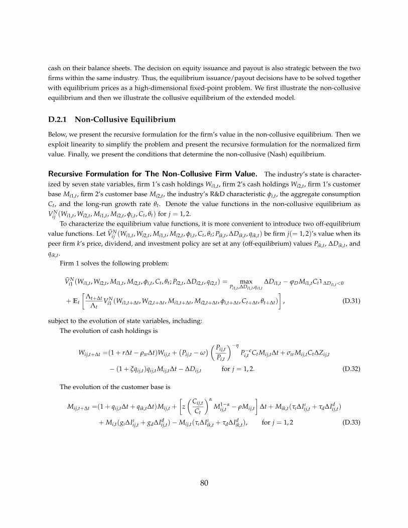
cash on their balance sheets. The decision on equity issuance and payout is also strategic between the twofirms within the same industry. Thus, the equilibrium issuance/payout decisions have to be solved togetherwith equilibrium prices as a high-dimensional fixed-point problem. We first illustrate the non-collusiveequilibrium and then we illustrate the collusive equilibrium of the extended model.

D.2.1 Non-Collusive Equilibrium

Below, we present the recursive formulation for the firm’s value in the non-collusive equilibrium. Then weexploit linearity to simplify the problem and present the recursive formulation for the normalized firmvalue. Finally, we present the conditions that determine the non-collusive (Nash) equilibrium.

Recursive Formulation for The Non-Collusive Firm Value. The industry’s state is character-ized by seven state variables, firm 1’s cash holdings Wi1,t, firm 2’s cash holdings Wi2,t, firm 1’s customerbase Mi1,t, firm 2’s customer base Mi2,t, the industry’s R&D characteristic φi,t, the aggregate consumptionCt, and the long-run growth rate θt. Denote the value functions in the non-collusive equilibrium asVN

ij (Wi1,t, Wi2,t, Mi1,t, Mi2,t, φi,t, Ct, θt) for j = 1, 2.To characterize the equilibrium value functions, it is more convenient to introduce two off-equilibrium

value functions. Let VNij (Wi1,t, Wi2,t, Mi1,t, Mi2,t, φi,t, Ct, θt; Pik,t, ∆Dik,t, qik,t) be firm j(= 1, 2)’s value when its

peer firm k’s price, dividend, and investment policy are set at any (off-equilibrium) values Pik,t, ∆Dik,t, andqik,t.

Firm 1 solves the following problem:

VNi1 (Wi1,t, Wi2,t, Mi1,t, Mi2,t, φi,t, Ct, θt; Pi2,t, ∆Di2,t, qi2,t) = max

Pi1,t ,∆Di1,t ,qi1,t∆Di1,t − ϕD Mi1,tCt1∆Di1,t<0

+ Et

[Λt+∆t

ΛtVN

i1 (Wi1,t+∆t, Wi2,t+∆t, Mi1,t+∆t, Mi2,t+∆t, φi,t+∆t, Ct+∆t, θt+∆t)

], (D.31)

subject to the evolution of state variables, including:The evolution of cash holdings is

Wij,t+∆t =(1 + r∆t− ρw∆t)Wij,t +(

Pij,t −ω) (Pij,t

Pi,t

)−η

P−εi,t Ct Mij,t∆t + σw Mij,tCt∆Zij,t

− (1 + ξqij,t)qij,t Mij,t∆t− ∆Dij,t for j = 1, 2. (D.32)

The evolution of the customer base is

Mij,t+∆t =(1 + qij,t∆t + qik,t∆t)Mij,t +

[z(Cij,t

Ct

)α

M1−αij,t − ρMij,t

]∆t + Mik,t(τι∆I ι

ij,t + τd∆Idij,t)

+ Mi,t(gι∆I ιij,t + gd∆Id

ij,t)−Mij,t(τι∆I ιik,t + τd∆Id

ik,t), for j = 1, 2 (D.33)

80

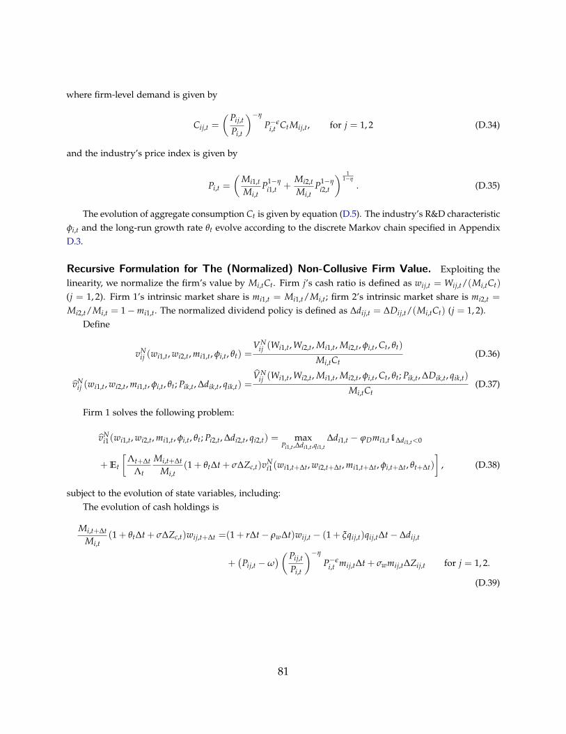
where firm-level demand is given by

Cij,t =

(Pij,t

Pi,t

)−η

P−εi,t Ct Mij,t, for j = 1, 2 (D.34)

and the industry’s price index is given by

Pi,t =

(Mi1,t

Mi,tP1−η

i1,t +Mi2,t

Mi,tP1−η

i2,t

) 11−η

. (D.35)

The evolution of aggregate consumption Ct is given by equation (D.5). The industry’s R&D characteristicφi,t and the long-run growth rate θt evolve according to the discrete Markov chain specified in AppendixD.3.

Recursive Formulation for The (Normalized) Non-Collusive Firm Value. Exploiting thelinearity, we normalize the firm’s value by Mi,tCt. Firm j’s cash ratio is defined as wij,t = Wij,t/(Mi,tCt)

(j = 1, 2). Firm 1’s intrinsic market share is mi1,t = Mi1,t/Mi,t; firm 2’s intrinsic market share is mi2,t =

Mi2,t/Mi,t = 1−mi1,t. The normalized dividend policy is defined as ∆dij,t = ∆Dij,t/(Mi,tCt) (j = 1, 2).Define

vNij (wi1,t, wi2,t, mi1,t, φi,t, θt) =

VNij (Wi1,t, Wi2,t, Mi1,t, Mi2,t, φi,t, Ct, θt)

Mi,tCt(D.36)

vNij (wi1,t, wi2,t, mi1,t, φi,t, θt; Pik,t, ∆dik,t, qik,t) =

VNij (Wi1,t, Wi2,t, Mi1,t, Mi2,t, φi,t, Ct, θt; Pik,t, ∆Dik,t, qik,t)

Mi,tCt(D.37)

Firm 1 solves the following problem:

vNi1(wi1,t, wi2,t, mi1,t, φi,t, θt; Pi2,t, ∆di2,t, qi2,t) = max

Pi1,t ,∆di1,t ,qi1,t∆di1,t − ϕDmi1,t1∆di1,t<0

+ Et

[Λt+∆t

Λt

Mi,t+∆t

Mi,t(1 + θt∆t + σ∆Zc,t)vN

i1(wi1,t+∆t, wi2,t+∆t, mi1,t+∆t, φi,t+∆t, θt+∆t)

], (D.38)

subject to the evolution of state variables, including:The evolution of cash holdings is

Mi,t+∆t

Mi,t(1 + θt∆t + σ∆Zc,t)wij,t+∆t =(1 + r∆t− ρw∆t)wij,t − (1 + ξqij,t)qij,t∆t− ∆dij,t

+(

Pij,t −ω) (Pij,t

Pi,t

)−η

P−εi,t mij,t∆t + σwmij,t∆Zij,t for j = 1, 2.

(D.39)

81

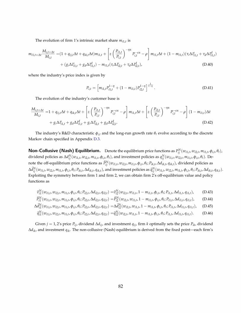
The evolution of firm 1’s intrinsic market share mi1,t is

mi1,t+∆tMi,t+∆t

Mi,t=(1 + qij,t∆t + qik,t∆t)mi1,t +

[z(

Pi1,t

Pi,t

)−ηα

P−εαi,t − ρ

]mi1,t∆t + (1−mi1,t)(τι∆I ι

i1,t + τd∆Idi1,t)

+ (gι∆I ιi1,t + gd∆Id

i1,t)−mi1,t(τι∆I ιi2,t + τd∆Id

i2,t), (D.40)

where the industry’s price index is given by

Pi,t =[mi1,tP

1−ηi1,t + (1−mi1,t)P1−η

i2,t

] 11−η . (D.41)

The evolution of the industry’s customer base is

Mi,t+∆t

Mi,t=1 + qij,t∆t + qik,t∆t +

[z(

Pi1,t

Pi,t

)−ηα

P−εαi,t − ρ

]mi1,t∆t +

[z(

Pi2,t

Pi,t

)−ηα

P−εαi,t − ρ

](1−mi1,t)∆t

+ gι∆I ιi1,t + gd∆Id

i1,t + gι∆I ιi2,t + gd∆Id

i2,t. (D.42)

The industry’s R&D characteristic φi,t and the long-run growth rate θt evolve according to the discreteMarkov chain specified in Appendix D.3.

Non-Collusive (Nash) Equilibrium. Denote the equilibrium price functions as PNij (wi1,t, wi2,t, mi1,t, φi,t, θt),

dividend policies as ∆dNij (wi1,t, wi2,t, mi1,t, φi,t, θt), and investment policies as qN

ij (wi1,t, wi2,t, mi1,t, φi,t, θt). De-

note the off-equilibrium price functions as PNij (wi1,t, wi2,t, mi1,t, φi,t, θt; Pik,t, ∆dik,t, qik,t), dividend policies as

∆dNij (wi1,t, wi2,t, mi1,t, φi,t, θt; Pik,t, ∆dik,t, qik,t), and investment policies as qN

ij (wi1,t, wi2,t, mi1,t, φi,t, θt; Pik,t, ∆dik,t, qik,t).Exploiting the symmetry between firm 1 and firm 2, we can obtain firm 2’s off-equilibrium value and policyfunctions as

vNi1(wi1,t, wi2,t, mi1,t, φi,t, θt; Pi2,t, ∆di2,t, qi2,t) =vN

i2(wi2,t, wi1,t, 1−mi1,t, φi,t, θt; Pi1,t, ∆di1,t, qi1,t), (D.43)

PNi1 (wi1,t, wi2,t, mi1,t, φi,t, θt; Pi2,t, ∆di2,t, qi2,t) =PN

i2 (wi2,t, wi1,t, 1−mi1,t, φi,t, θt; Pi1,t, ∆di1,t, qi1,t), (D.44)

∆dNi1(wi1,t, wi2,t, mi1,t, φi,t, θt; Pi2,t, ∆di2,t, qi2,t) =∆dN

i2(wi2,t, wi1,t, 1−mi1,t, φi,t, θt; Pi1,t, ∆di1,t, qi1,t), (D.45)

qNi1(wi1,t, wi2,t, mi1,t, φi,t, θt; Pi2,t, ∆di2,t, qi2,t) =qN

i2(wi2,t, wi1,t, 1−mi1,t, φi,t, θt; Pi1,t, ∆di1,t, qi1,t). (D.46)

Given j = 1, 2’s price Pij, dividend ∆dij, and investment qij, firm k optimally sets the price Pik, dividend∆dik, and investment qik. The non-collusive (Nash) equilibrium is derived from the fixed point—each firm’s

82

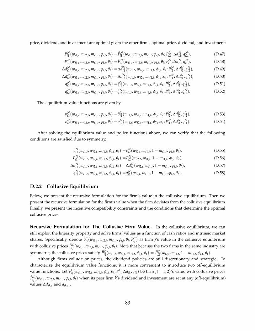
price, dividend, and investment are optimal given the other firm’s optimal price, dividend, and investment:

PNi1 (wi1,t, wi2,t, mi1,t, φi,t, θt) =PN

i1 (wi1,t, wi2,t, mi1,t, φi,t, θt; PNi2 , ∆dN

i2 , qNi2), (D.47)

PNi2 (wi1,t, wi2,t, mi1,t, φi,t, θt) =PN

i2 (wi1,t, wi2,t, mi1,t, φi,t, θt; PNi1 , ∆dN

i1 , qNi1), (D.48)

∆dNi1(wi1,t, wi2,t, mi1,t, φi,t, θt) =∆dN

i1(wi1,t, wi2,t, mi1,t, φi,t, θt; PNi2 , ∆dN

i2 , qNi2), (D.49)

∆dNi2(wi1,t, wi2,t, mi1,t, φi,t, θt) =∆dN

i2(wi1,t, wi2,t, mi1,t, φi,t, θt; PNi1 , ∆dN

i1 , qNi1), (D.50)

qNi1(wi1,t, wi2,t, mi1,t, φi,t, θt) =qN

i1(wi1,t, wi2,t, mi1,t, φi,t, θt; PNi2 , ∆dN

i2 , qNi2), (D.51)

qNi2(wi1,t, wi2,t, mi1,t, φi,t, θt) =qN

i2(wi1,t, wi2,t, mi1,t, φi,t, θt; PNi1 , ∆dN

i1 , qNi1). (D.52)

The equilibrium value functions are given by

vNi1(wi1,t, wi2,t, mi1,t, φi,t, θt) =vN

i1(wi1,t, wi2,t, mi1,t, φi,t, θt; PNi2 , ∆dN

i2 , qNi2), (D.53)

vNi2(wi1,t, wi2,t, mi1,t, φi,t, θt) =vN

i2(wi1,t, wi2,t, mi1,t, φi,t, θt; PNi1 , ∆dN

i1 , qNi1). (D.54)

After solving the equilibrium value and policy functions above, we can verify that the followingconditions are satisfied due to symmetry,

vNi1(wi1,t, wi2,t, mi1,t, φi,t, θt) =vN

i2(wi2,t, wi1,t, 1−mi1,t, φi,t, θt), (D.55)

PNi1 (wi1,t, wi2,t, mi1,t, φi,t, θt) =PN

i2 (wi2,t, wi1,t, 1−mi1,t, φi,t, θt), (D.56)

∆dNi1(wi1,t, wi2,t, mi1,t, φi,t, θt) =∆dN

i2(wi2,t, wi1,t, 1−mi1,t, φi,t, θt), (D.57)

qNi1(wi1,t, wi2,t, mi1,t, φi,t, θt) =qN

i2(wi2,t, wi1,t, 1−mi1,t, φi,t, θt). (D.58)

D.2.2 Collusive Equilibrium

Below, we present the recursive formulation for the firm’s value in the collusive equilibrium. Then wepresent the recursive formulation for the firm’s value when the firm deviates from the collusive equilibrium.Finally, we present the incentive compatibility constraints and the conditions that determine the optimalcollusive prices.

Recursive Formulation for The Collusive Firm Value. In the collusive equilibrium, we canstill exploit the linearity property and solve firms’ values as a function of cash ratios and intrinsic marketshares. Specifically, denote vC

ij(wi1,t, wi2,t, mi1,t, φi,t, θt; PCij ) as firm j’s value in the collusive equilibrium

with collusive prices PCij (wi1,t, wi2,t, mi1,t, φi,t, θt). Note that because the two firms in the same industry are

symmetric, the collusive prices satisfy PCi1(wi1,t, wi2,t, mi1,t, φi,t, θt) = PC

i2(wi2,t, wi1,t, 1−mi1,t, φi,t, θt).Although firms collude on prices, the dividend policies are still discretionary and strategic. To

characterize the equilibrium value functions, it is more convenient to introduce two off-equilibriumvalue functions. Let vC

ij(wi1,t, wi2,t, mi1,t, φi,t, θt; PCij , ∆dik, qik) be firm j(= 1, 2)’s value with collusive prices

PCij (wi1,t, wi2,t, mi1,t, φi,t, θt) when its peer firm k’s dividend and investment are set at any (off-equilibrium)

values ∆dik,t and qik,t .

83

Firm 1 solves the following normalized problem:

vCi1(wi1,t, wi2,t, mi1,t, φi,t, θt; PC

ij , ∆di2,t, qi2,t) = max∆di1,t ,qi1,t

∆di1,t − ϕDmi1,t1∆di1,t<0

+ Et

[Λt+∆t

Λt

Mi,t+∆t

Mi,t(1 + θt∆t + σ∆Zc,t)vC

i1(wi1,t+∆t, wi2,t+∆t, mi1,t+∆t, φi,t+∆t, θt+∆t; PCij )

], (D.59)

subject to the evolution of state variables, including:The evolution of cash ratios is

Mi,t+∆t

Mi,t(1 + θt∆t + σ∆Zc,t)wij,t+∆t = (1 + r∆t− ρw∆t)wij,t − (1 + ξqij,t)qij,t∆t− ∆dij,t

+(

PCij (wi1,t, wi2,t, mi1,t, φi,t, θt)−ω

)( PCij (wi1,t, wi2,t, mi1,t, φi,t, θt)

Pi,t

)−η

P−εi,t mij,t∆t + σwmij,t∆Zij,t for j = 1, 2.

(D.60)

The evolution of firm 1’s intrinsic market share mi1,t is

mi1,t+∆tMi,t+∆t

Mi,t=(1 + qi1,t∆t + qi2,t∆t)mi1,t +

z

(PC

i1(mi1,t, φi,t, θt)

Pi,t

)−ηα

P−εαi,t − ρ

mi1,t∆t

+ (1−mi1,t)(τι∆I ιi1,t + τd∆Id

i1,t) + (gι∆I ιi1,t + gd∆Id

i1,t)−mi1,t(τι∆I ιi2,t + τd∆Id

i2,t), (D.61)

where the industry’s price index is given by

Pi,t =[mi1,t PC

i1(mi1,t, φi,t, θt)1−η + (1−mi1,t)PC

i2(mi1,t, φi,t, θt)1−η] 1

1−η . (D.62)

The evolution of the industry’s customer base is

Mi,t+∆t

Mi,t=1 +

z

(PC

i1(mi1,t, φi,t, θt)

Pi,t

)−ηα

P−εαi,t − ρ

mi1,t∆t +

z

(PC

i2(mi1,t, φi,t, θt)

Pi,t

)−ηα

P−εαi,t − ρ

(1−mi1,t)∆t

+ qi1,t∆t + qi2,t∆t + gι∆I ιi1,t + gd∆Id

i1,t + gι∆I ιi2,t + gd∆Id

i2,t. (D.63)

The industry’s R&D characteristic φi,t and the long-run growth rate θt evolve according to the discreteMarkov chain specified in Appendix D.3.

Next, we characterize dividend and investment policies in collusive equilibrium. Denote the equilibriumdividend policies as ∆dC

ij(wi1,t, wi2,t, mi1,t, φi,t, θt; PCij ) and investment policies as qC

ij(wi1,t, wi2,t, mi1,t, φi,t, θt; PCij ).

Denote the off-equilibrium dividend policies as ∆dCij(wi1,t, wi2,t, mi1,t, φi,t, θt; PC

ij , ∆dik,t, qik,t) and investment

policies as qCij(wi1,t, wi2,t, mi1,t, φi,t, θt; PC

ij , ∆dik,t, qik,t). Exploiting the symmetry between firm 1 and firm 2,

84

we can obtain firm 2’s off-equilibrium value and policy functions as

vCi1(wi1,t, wi2,t, mi1,t, φi,t, θt; PC

ij , ∆di2,t, qi2,t) =vCi2(wi2,t, wi1,t, 1−mi1,t, φi,t, θt; PC

ij , ∆di1,t, qi1,t), (D.64)

∆dCi1(wi1,t, wi2,t, mi1,t, φi,t, θt; PC

ij , ∆di2,t, qi2,t) =∆dCi2(wi2,t, wi1,t, 1−mi1,t, φi,t, θt; PC

ij , ∆di1,t, qi1,t), (D.65)

qCi1(wi1,t, wi2,t, mi1,t, φi,t, θt; PC

ij , ∆di2,t, qi2,t) =qCi2(wi2,t, wi1,t, 1−mi1,t, φi,t, θt; PC

ij , ∆di1,t, qi1,t). (D.66)

Given j = 1, 2’s dividend ∆dij and investment qij, firm k optimally sets its dividend ∆dik and investmentqik. The collusive-equilibrium dividend and investment policies are derived from the fixed points—eachfirm’s dividend and investment policies are optimal given the other firm’s dividend and investment policies:

∆dCi1(wi1,t, wi2,t, mi1,t, φi,t, θt; PC

ij ) =∆dCi1(wi1,t, wi2,t, mi1,t, φi,t, θt; PC

ij , ∆dCi2, qC

i2), (D.67)

∆dCi2(wi1,t, wi2,t, mi1,t, φi,t, θt; PC

ij ) =∆dCi2(wi1,t, wi2,t, mi1,t, φi,t, θt; PC

ij , ∆dCi1, qC

i1), (D.68)

qCi1(wi1,t, wi2,t, mi1,t, φi,t, θt; PC

ij ) =qCi1(wi1,t, wi2,t, mi1,t, φi,t, θt; PC

ij , ∆dCi2, qC

i2), (D.69)

qCi2(wi1,t, wi2,t, mi1,t, φi,t, θt; PC

ij ) =qCi2(wi1,t, wi2,t, mi1,t, φi,t, θt; PC

ij , ∆dCi1, qC

i1). (D.70)

The equilibrium value functions are given by

vCi1(wi1,t, wi2,t, mi1,t, φi,t, θt; PC

ij ) =vCi1(wi1,t, wi2,t, mi1,t, φi,t, θt; PC

ij , ∆dCi2, qC

i2), (D.71)

vCi2(wi1,t, wi2,t, mi1,t, φi,t, θt; PC

ij ) =vCi2(wi1,t, wi2,t, mi1,t, φi,t, θt; PC

ij , ∆dCi1, qC

i1). (D.72)

After solving the equilibrium value and policy functions above, we can verify that the followingconditions are satisfied due to symmetry,

vCi1(wi1,t, wi2,t, mi1,t, φi,t, θt; PC

ij ) =vCi2(wi2,t, wi1,t, 1−mi1,t, φi,t, θt; PC

ij ), (D.73)

∆dCi1(wi1,t, wi2,t, mi1,t, φi,t, θt; PC

ij ) =∆dCi2(wi2,t, wi1,t, 1−mi1,t, φi,t, θt; PC

ij ), (D.74)

qCi1(wi1,t, wi2,t, mi1,t, φi,t, θt; PC

ij ) =qCi2(wi2,t, wi1,t, 1−mi1,t, φi,t, θt; PC

ij ). (D.75)

Recursive Formulation for The Deviation Value. The deviation value is obtained by assumingthat firm j optimally sets its price, dividend, and investment policies conditional on firm k not knowingthat deviation has happened. Thus, firm k remains setting price PC

ik(wi1,t, wi2,t, mi1,t, φi,t, θt), dividend∆dC

ik(wi1,t, wi2,t, mi1,t, φi,t, θt; PCij ), and investment qC

ik(wi1,t, wi2,t, mi1,t, φi,t, θt; PCij ) as in the collusive equilib-

rium. We exploit the linearity property and solve firms’ deviation values as a function of intrinsic marketshares. Denote vD

ij (wi1,t, wi2,t, mi1,t, φi,t, θt; PCij ) as firm j’s deviation value.

Firm 1 solves the following problem:

vDi1(wi1,t, wi2,t, mi1,t, φi,t, θt; PC

ij ) = maxPi1,t ,∆di1,t ,qi1,t

∆di1,t − ϕDmi1,t1∆di1,t<0 + Et

[Λt+∆t

Λt

Mi,t+∆t

Mi,t(1 + θt∆t + σ∆Zc,t)

×[(1− ς∆t)vD

i1(wi1,t+∆t, wi2,t+∆t, mi1,t+∆t, φi,t+∆t, θt+∆t; PCij ) + ς∆tvN

i1(wi1,t+∆t, wi2,t+∆t, mi1,t+∆t, φi,t+∆t, θt+∆t)]]

,

(D.76)

85

subject to the evolution of state variables, including:The evolution of firm 1’s cash holdings is

Mi,t+∆t

Mi,t(1 + θt∆t + σ∆Zc,t)wi1,t+∆t =(1 + r∆t− ρw∆t)wi1,t − (1 + ξqi1,t)qi1,t∆t− ∆di1,t

+ (Pi1,t −ω)

(Pi1,t

Pi,t

)−η

P−εi,t mi1,t∆t + σwmi1,t∆Zi1,t. (D.77)

The evolution of firm 2’s cash holdings is

Mi,t+∆t

Mi,t(1 + θt∆t + σ∆Zc,t)wi2,t+∆t = (1 + r∆t− ρw∆t)wi2,t − ∆dC

i2(wi1,t, wi2,t, mi1,t, φi,t, θt; PCij )

− [1 + ξ qCi2(wi1,t, wi2,t, mi1,t, φi,t, θt; PC

ij )]qCi2(wi1,t, wi2,t, mi1,t, φi,t, θt; PC

ij )∆t

+(

PCi2(wi1,t, wi2,t, mi1,t, φi,t, θt)−ω

)( PCi2(wi1,t, wi2,t, mi1,t, φi,t, θt)

Pi,t

)−η

P−εi,t (1−mi1,t)∆t + σw(1−mi1,t)∆Zi2,t.

(D.78)

The evolution of firm 1’s intrinsic market share is

mi1,t+∆tMi,t+∆t

Mi,t=[1 + qi1,t∆t + qC

i2(wi1,t, wi2,t, mi1,t, φi,t, θt; PCij )∆t]mi1,t +

[z(

Pi1,t

Pi,t

)−ηα

P−εαi,t − ρ

]mi1,t∆t

+ (1−mi1,t)(τι∆I ιi1,t + τd∆Id

i1,t) + (gι∆I ιi1,t + gd∆Id

i1,t)−mi1,t(τι∆I ιi2,t + τd∆Id

i2,t), (D.79)

where the industry’s price index is given by

Pi,t =[mi1,tP

1−ηi1,t + (1−mi1,t)PC

i2(mi1,t, φi,t, θt)1−η] 1

1−η . (D.80)

The evolution of the industry’s customer base is

Mi,t+∆t

Mi,t=1 + qi1,t∆t + qC

i2(wi1,t, wi2,t, mi1,t, φi,t, θt; PCij )∆t + gι∆I ι

i1,t + gd∆Idi1,t + gι∆I ι

i2,t + gd∆Idi2,t.

+

[z(

Pi1,t

Pi,t

)−ηα

P−εαi,t − ρ

]mi1,t∆t +

z

(PC

i2(mi1,t, φi,t, θt)

Pi,t

)−ηα

P−εαi,t − ρ

(1−mi1,t)∆t.

(D.81)

The industry’s R&D characteristic φi,t and the long-run growth rate θt evolve according to the discreteMarkov chain specified in Appendix D.3.

Incentive Compatibility Constraints and Optimal Collusive Prices. The collusive equilib-rium is a sub-game perfect equilibrium if and only if the collusive prices PC

ij (wi1,t, wi2,t, mi1,t, φi,t, θt) satisfy

86

the following incentive compatibility constraints:

vCij(wi1,t, wi2,t, mi1,t, φi,t, θt; PC

ij ) ≥ vDij (wi1,t, wi2,t, mi1,t, φi,t, θt; PC

ij ), (D.82)

for all wi1,t, wi2,t > 0, mi1,t ∈ [0, 1], φi,t ∈ Φ, θt, and j = 1, 2.There exist infinitely many sub-game perfect collusive equilibrium. We focus on the collusive equilib-

rium with the highest collusive prices (denoted by PCij (wi1,t, wi2,t, mi1,t, φi,t, θt)), which are obtained when

all incentive compatibility constraints are binding, i.e.

vCij(wi1,t, wi2,t, mi1,t, φi,t, θt; PC

ij ) = vDij (wi1,t, wi2,t, mi1,t, φi,t, θt; PC

ij ), (D.83)

for all wi1,t, wi2,t > 0, mi1,t ∈ [0, 1], φi,t ∈ Φ, θt, and j = 1, 2. We denote vCij(wi1,t, wi2,t, mi1,t, φi,t, θt) as firm

j’s value in the collusive equilibrium with collusive prices PCij (wi1,t, wi2,t, mi1,t, φi,t, θt), thus by definition

vCij(wi1,t, wi2,t, mi1,t, φi,t, θt) = vC

ij(wi1,t, wi2,t, mi1,t, φi,t, θt; PCij ). (D.84)

D.3 DiscretizationWe discretize the cash flow shocks dZij,t based on n grids spanning from −3σ to 3σ, the unpredictableconsumption growth shocks dZc,t based on nc grids spanning from −3σc and 3σc using the method ofTauchen (1986). We use the method of Rouwenhorst (1995) to approximate the persistent AR(1) process oflong-run risks θt using nθ discrete states. The time line is discretized into intervals with length ∆t.

We use collocation methods to solve each firm’s problem. Let Sm × Sφ × Sθ be the grid of collocationnodes for a firm’s equilibrium value in the baseline model, Sm× Sφ× Sθ × Sp be the grid of collocation notesfor a firm’s off-equilibrium value in the baseline model, Sw × Sw × Sm × Sφ × Sθ be the grid of collocationnodes for a firm’s equilibrium value in the extended model, and Sw × Sw × Sm × Sφ × Sθ × Sp × Sd × Sq

be the grid of collocation nodes for a firm’s off-equilibrium value in the extended model. We have Sw =

{w1, w2, ..., wnw}, Sm = {m1, m2, ..., mnm}, Sφ = {φ1, φ2, ..., φnφ}, Sθ = {θ1, θ2, ..., θnθ}, Sp = {p1, p2, ..., pnp},

Sd = {d1, d2, ..., dnd}, and Sq = {q1, q2, ..., qnq}.We approximate the firm’s value function v(·) on the grid of collocation notes using a linear spline

with coefficients corresponding to each grid point. We first form a guess for the spline’s coefficients, thenwe iterate to obtain a vector that solves the system of Bellman equations. For our extended model, becausethere are three continuous endogenous states, Sw × Sw × Sm, we use the piecewise multilinear interpolationmethod of Weiser and Zarantonello (1988) to obtain interpolant in a 3-dimensional space.

D.4 ImplementationThe numerical algorithms are implemented using C++. The program is run on the server of MIT EconomicsDepartment, supply.mit.edu and demand.mit.edu, which are built on Dell PowerEdge R910 (64 cores, Intel(R)Xeon(R) CPU E7-4870, 2.4GHz) and Dell PowerEdge R920 (48 cores, Intel(R) 4 Xeon E7-8857 v2 CPUs). Weuse OpenMP for parallelization when iterating value functions and simulating the model.

87

Selection of Grids For our baseline model, we set nc = 11, nθ = 21, nm = 21, ∆t = 1/24, nφ = 11,np = 11. The grids for long-run risks Sθ is given by the method of Rouwenhorst (1995). The grids forunpredictable consumption growth shocks Sc is given by the method of Tauchen (1986). The grid of intrinsicmarket share Sm is discretized into 21 nodes from 1e− 7 to 1− 1e− 7 with equal spaces. We do not set Sm

from 0 to 1 to avoid the indeterminacy of optimal price with m = 0. The time interval ∆t is set to be 1/24.A higher ∆t implies faster convergence for the same number of iterations but lower accuracy. We checkedthat the solution is accurate enough for ∆t = 1/24, further reducing ∆t would not change the accuracymuch. With 1/24, 5000 times iterations allow us to achieve convergence in value functions. The industrycharacteristic grid is discretized into 11 notes from 0 to 1 with equal spaces. The price grids is discretizedinto 11 nodes from 1 to 2 with equal spaces. The upper bound is chosen according to ε/(ε− 1)×ω = 2,which is the highest price a firm will ever set.

For our extended model, we set nc = 3, nθ = 3, nm = 21, ∆t = 1/365, nφ = 11, np = 11, n = 5, nw = 26,nd = 3, nq = 3. The extended model is much more difficult to compute due to endogenous cash holdings.Thus, to ensure we can solve the model within a reasonable amount of time, we reduce the number ofnodes for unpredictable consumption growth shocks to 3, and reduce the number of nodes for long-runrisks to 3. To ensure accuracy, we keep the number of nodes for intrinsic market shares unchanged at21, and the number of price nodes unchanged at 11. We use nw = 26 equi-spaced nodes from 0 to 0.5 toconstruct Sw, which is dense enough to capture the nonlinearity in marginal value of cash. We set use n = 5to approximate cash flow shocks. We have tested that further reducing n would not be able to generatesufficient cash flow risks due to discretization error, although it increases the speed of computation. Notethat with endogenous cash holdings, we cannot set ∆ = 1/24 because the discretized cash flow shock withrelatively larger ∆ could exceed the upper bound of our cash holding grids. Thus, there is a tradeoff. If weuse more grids for Sw to have higher upper bound, we can choose relatively larger ∆ to save iteration time.However, each iteration will take longer. Given our grids nw = 26 and upper bound of w equal to 0.5, wehave to choose ∆ = 1/365 in order to maintain reasonable accuracy. With ∆ = 1/365, 20000 iterations areneeded for value function convergence.

Calculating Iterations and Searching For the Nash Equilibrium. Given the value functionsfrom the previous iteration, we use the golden section search method to find the equilibrium prices. Thecomputational complexity of this algorithm is at the order of log(n), much faster and more accurate than asimple grid search.

Searching for the equilibrium markup is very difficult because we have to solve a fixed-point problem(D.47-D.54) that involves both firms’ simultaneous prices and net payout decisions. Our solution techniqueis to iteratively solve the following three steps.

First, given vNi1(wi1, wi2, mi1, φi, θ), we solve for the off-equilibrium value vN

i1(wi1, wi2, mi1, φi, θ; Pi2, ∆di2, qi2),the off-equilibrium policy functions PN

i1 (wi1, wi2, mi1, φi, θ; Pi2, ∆di2, qi2), ∆dNi1(wi1, wi2, mi1, φi, θ; Pi2, ∆di2, qi2),

qNi1(wi1, wi2, mi1, φi, θ; Pi2, ∆di2, qi2). Exploiting symmetry, we obtain vN

i2(wi1, wi2, mi1, φi, θ; Pi1, ∆di1, qi1), andPN

i2 (wi1, wi2, mi1, φi, θ; Pi1, ∆di1, qi1), ∆dNi2(wi1, wi2, mi1, φi, θ; Pi1, ∆di1, qi1), qN

i2(wi1, wi2, mi1, φi, θ; Pi1, ∆di1, qi1).Second, for each (wi1, wi2, mi1, φi, θ) ∈ Sw × Sw × Sm × Sφ × Sθ , we use a nonlinear solver knitro to

solve equations (D.47-D.52) and obtain the equilibrium prices PNi1 (wi1, wi2, mi1, φi, θ), PN

i1 (wi2, wi2, mi1, φi, θ),

88

the equilibrium net payout ddNi1(wi1, wi2, mi1, φi, θ), ddN

i2(wi1, wi2, mi1, φi, θ), and the equilibrium investmentqN

i1(wi1, wi2, mi1, φi, θ), qNi2(wi1, wi2, mi1, φi, θ). Third, we solve equations (D.53-D.54) and obtain equilibrium

value functions vNi1(wi1, wi2, mi1, φi, θ), and vN

i2(wi1, wi2, mi1, φi, θ).Searching for the optimal net payout is also difficult because financing and payout only happen at

the boundaries when time is continuous. There are two complications when solving this continuous-timemodel in discrete time. First, the firm starts to issue equity in advance before the cash ratio hits the zerolower bound. Second, the discretized cash flow shocks may drive the next-period cash ratio to a negativenumber even when the firm’s current-period cash ratio is strictly positive. We deal with the first problemby choosing a fine time grid, i.e. ∆ = 1/365. This ensures a reasonably good approximation as the firmissues equity when cash ratio drops below 0.02, the smallest cash ratio grid we consider. To deal withthe second issue, we impose a sufficiently large penalty on the firm’s value (in the code, we subtract thefirm’s value by 10) whenever the next-period cash ratio drops below zero. This is to ensure that the firmwould issue equity whenever there is a chance to have a negative cash ratio in the next period given ourdiscretization of cash flow shocks. The large penalty is important to guarantee the convergence of the valuefunctions. If the penalty is not large enough, then the firm may wait for a bit longer before issuing equity,and as a result, the optimal financing boundary is not correctly solved at this level of discretization.

Searching For Collusive Prices. We modify the golden section search method to find the highestcollusive prices PC(wi1, wi2, mi1, φi, θ) by iterations. Within each iteration, we solve firms’ collusion valueand deviation value using standard recursive methods given PC

ij (wi1, wi2, mi1, φi, θ).There are two key differences between our method and a standard golden section search method.

First, we guess and update the collusive pricing schedule PCij (wi1, wi2, mi1, φi, θ) simultaneously for all

(wi1, wi2, mi1, φi, θ) ∈ Sw × Sw × Sm × Sφ × Sθ , instead of doing it one by one for each state. This is toincrease efficiency. But, a natural problem introduced by the simultaneous updating is that there mightbe overshooting. For example, if for some particular state (w∗, w∗, m∗, φ∗, θ∗), we updated a collusiveprice PC

ij (w∗, w∗, m∗, φ∗, θ∗) too high in the previous iteration, the collusive price for some other states

(w, w, m, φ, θ) 6= (w∗, w∗, m∗, φ∗, θ∗) might be affected in this iteration and never achieve a binding incentivecompatibility constraint. Eventually, this may lead to non-convergence.

We solve this problem by gradually updating the collusive prices. In particular, in each roundof iteration, we first compute the updated collusive pricing schedule PC′

ij (wi1, wi2, mi1, φi, θ) impliedby the golden section search method. Then, instead of changing the upper search bound or lowersearch bound to PC′

ij (wi1, wi2, mi1, φi, θ) directly, we change it to (1− adj)× PCij (wi1, wi2, mi1, φi, θ) + adj×

PC′ij (wi1, wi2, mi1, φi, θ), a weighted average of the current collusive price PC

ij (wi1, wi2, mi1, φi, θ) and the

updated collusive price PC′ij (wi1, wi2, mi1, φi, θ). For our baseline model, we set adj = 0.3 to ensure perfect

convergence. For our extended model, due to larger nonlinearity, we change adj = 0.1 to obtain perfectconvergence.

89