ACCIDENT DATA AND THE PASSIVE SAFETY OF VEHICLES

OR

CAN YOU RATE THE PASSIVE SAFETY OF VEHICLES FROM ACCIDENT DATA?

ABSTRACT

Robert Zobel Volkswagen AG

The purpose of this paper is to report on a study made by Volkswagen, comparing the results from different institutes on the passive safety of vehicles. These institutes use accident data from the police or from insurance companies. They derive a rating from these figures and publish it as a guideline for the customer, "to choose safety."

At least their publications seek to give this impression:

Title of the leaflet of the British Ministry of Transportation: Buying a Car? Choose Safety.

The Australian Monash University Accident Research Centre uses the title: How does your car rate in a crash?

Folksam, a Swedish insurance company is very clear: How safe is your car?

Clearly they feel that their data can answer this question.

lt is the purpose of this paper to summarize a number of observations which make it hard to believe that we are already in a position to evaluate the passive safety of vehicles from accident statistics alone.

- 375 -

1 . Basic problems

The probability of an accident is influenced by a lot of factors. In principle, these are classified as driver-related, vehicle-related and environment-related. Two basic observations indicate, why these factors have to be considered very carefully.

lnfluence of Driving Environment to Fatality Rate

Total Urban Rural Autobahn

Road types

Average Only autobahn Only rural Only urban Primarily autobahn Primarily rural Primarily urban Equally distributed

West Germany 1 993 Bill ion Fatalities

vehicle-ki lometres

485.7 1 42.4 1 92.9 1 50.4

4080 465

2971 647

Rate

8.4 3 .3 1 5.4 4.3

Distribution of road types in % urban rural autobahn 29.3 39.7 31 .0 0.0 0.0 1 00.0 0.0 1 00.0 0.0

1 00.0 0.0 0.0 20.0 20.0 60.0 20.0 60.0 20.0 60.0 20.0 20.0 33.3 33.3 33.3

Rate

8.4 4.3 1 5.4 3.3 6.3 1 0.8 5.9 7.7

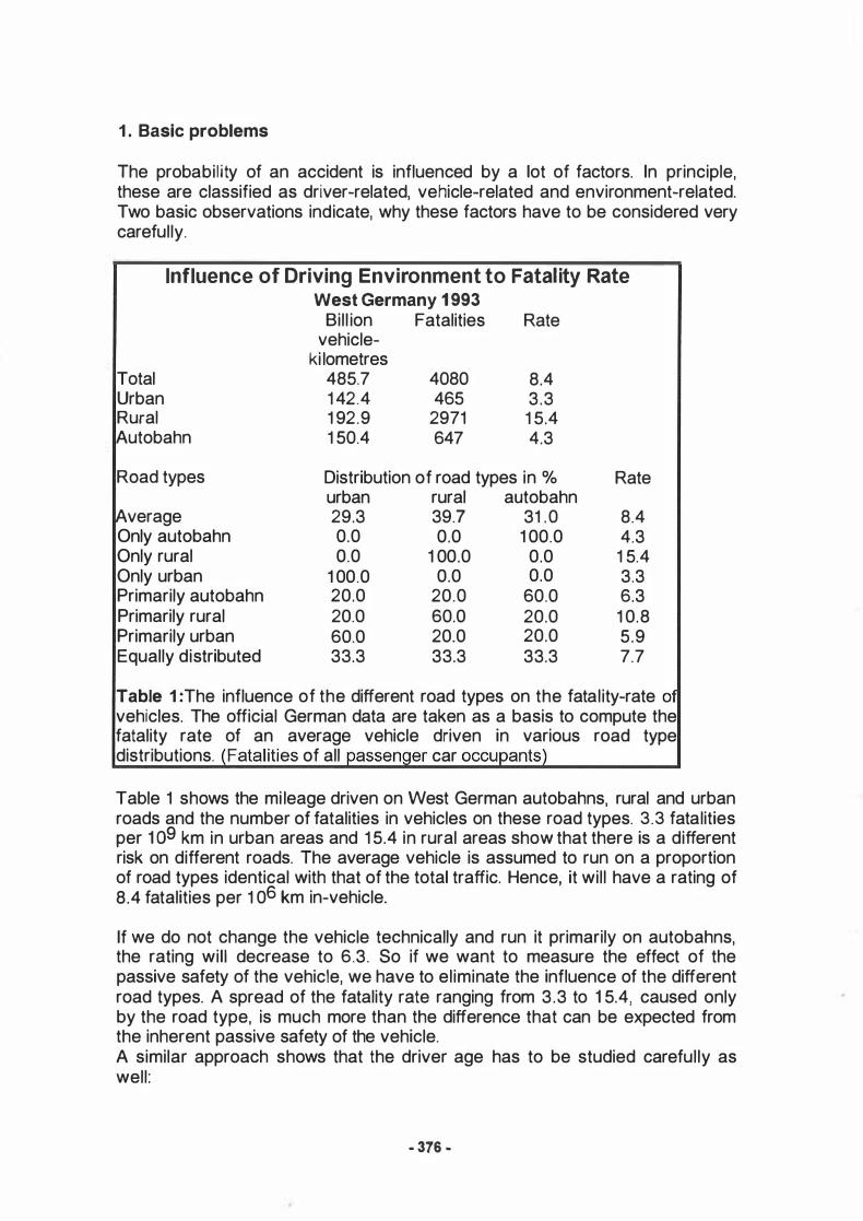
Table 1 :The influence of the different road types on the fatality-rate o1 vehicles. The official German data are taken as a basis to compute the fatality rate of an average vehicle driven in various road type distributions. (Fatalities of all passenQer car occupants)

Table 1 shows the mi leage driven on West German autobahns, rural and urban roads and the number of fatalities in vehicles on these road types. 3.3 fatalities per 1 o9 km in urban areas and 1 5.4 in rural areas show that there is a different risk on different roads. The average vehicle is assumed to run on a proportion of road types identical with that of the total traffic. Hence, it will have a rating of 8.4 fatalities per 1 06 km in-vehicle.

lf we do not change the vehicle technically and run it primarily on autobahns, the rating will decrease to 6.3. So if we want to measure the effect of the passive safety of the vehicle, we have to eliminate the influence of the different road types. A spread of the fatality rate ranging from 3.3 to 1 5.4, caused only by the road type, is much more than the difference that can be expected from the inherent passive safety of the vehicle. A similar approach shows that the driver age has to be studied carefully as well:

- 376 -

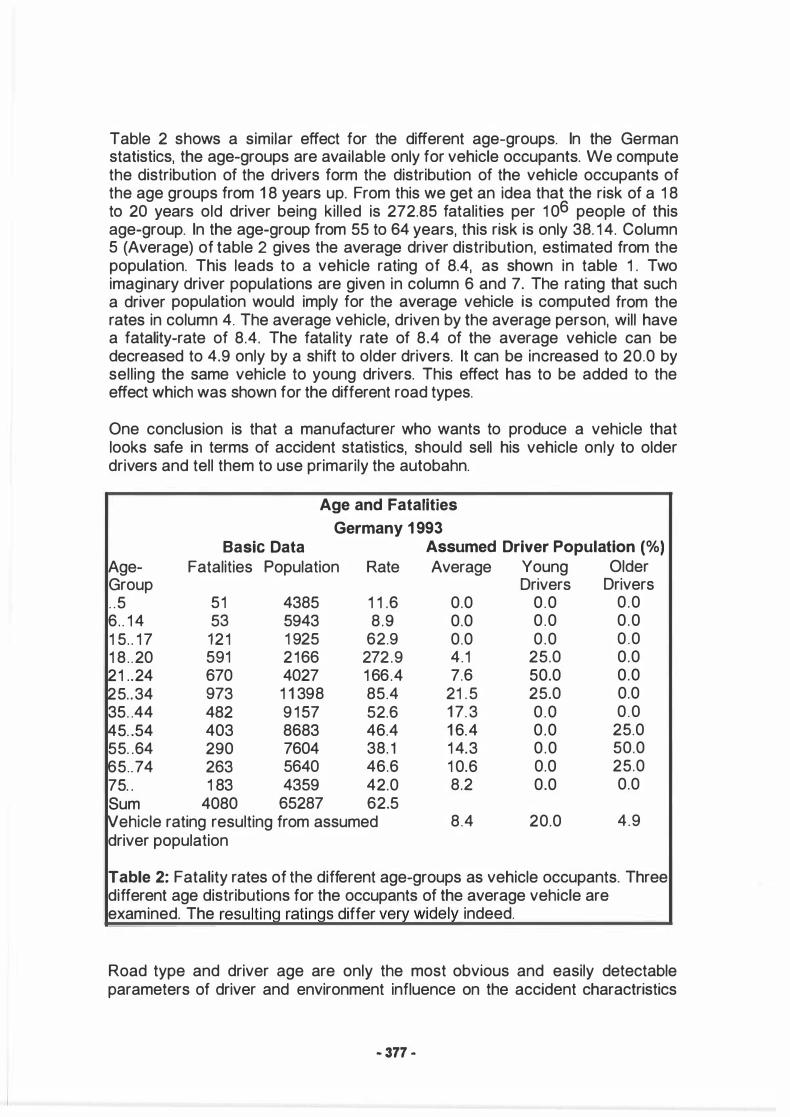
Table 2 shows a similar effect for the different age-groups. In the German statistics, the age-groups are available only for vehicle occupants. We compute the distribution of the drivers form the distribution of the vehicle occupants of the age groups from 1 8 years up. From this we get an idea that the risk of a 1 8 to 20 years old driver being killed is 272.85 fatalities per 1 06 people of this age-group. In the age-group from 55 to 64 years, this risk is only 38. 1 4. Column 5 (Average) of table 2 gives the average driver distribution, estimated from the population. This leads to a vehicle rating of 8.4, as shown in table 1 . Two imaginary driver populations are given in column 6 and 7. The rating that such a driver population would imply for the average vehicle is computed from the rates in column 4. The average vehicle, driven by the average person, will have a fatality-rate of 8.4. The fatality rate of 8.4 of the average vehicle can be decreased to 4.9 only by a shift to older drivers. lt can be increased to 20.0 by selling the same vehicle to young drivers. This effect has to be added to the effect which was shown for the different road types.

One conclusion is that a manufacturer who wants to produce a vehicle that looks safe in terms of accident statistics, should seil his vehicle only to older drivers and tell them to use primarily the autobahn.

Age and Fatalities

Germany 1 993 Basic Data Assumed Driver Population (%)

Age- Fatalities Population Rate Average Young Older Group Drivers Drivers . . 5 51 4385 1 1 .6 0.0 0 .0 0 .0 6 . . 1 4 53 5943 8.9 0.0 0 .0 0 .0 1 5 . . 1 7 121 1 925 62.9 0.0 0 .0 0 .0 1 8 . . 20 591 2166 272.9 4.1 25.0 0.0 21 . . 24 670 4027 1 66.4 7.6 50.0 0.0 25 . . 34 973 1 1 398 85.4 21 .5 25.0 0.0 35 . .44 482 9 1 57 52.6 1 7.3 0 .0 0 .0 45 . . 54 403 8683 46.4 1 6.4 0 .0 25.0 55 . . 64 290 7604 38. 1 1 4.3 0 .0 50.0 65 .. 74 263 5640 46.6 1 0.6 0.0 25.0 75 . . 1 83 4359 42.0 8.2 0.0 0.0 Sum 4080 65287 62.5 Vehicle rating resulting from assumed 8.4 20.0 4.9 driver population

Table 2: Fatality rates of the different age-groups as vehicle occupants. Three different age distributions for the occupants of the average vehicle are examined. The resultinq ratinqs differ very widely indeed.

Road type and driver age are only the most obvious and easily detectable parameters of driver and environment influence on the accident charactristics

• 377 .

of vehicles. Other parameters such as the probability of alcohol misuse in the driver population, personal behaviour in traffic, the number of traffic offences etc. are to be studied carefully as wei l . Otherwise a vehicle will be rated worse because of its drivers or the environment in which it is driven. The different regional and personal insurance premiums prove clearly that these differences are significant.

2. The double-pair approach

In 1 985, L. Evans from the General Motors Research Laboratories published a paper on "Double Pair Comparison: A New Method to Determine How Occupant Characteristics Affect Fatality Risk in Traffic Crashes." His main idea was to determine belt effectiveness by comparing the percentage of fatalities of belted drivers with the percentage of fatalities of unbelted drivers, where the crash severity was so high that the unbelted passenger was killed. Since he did not know the accident severity from the data file, he defined a severity threshold in line with whether or not the unbelted passenger was killed.

This method was adopted by Folksam researchers for use in vehicle rating.

They also define a severity threshold for crashes to be taken into account: They choose all collisions between a vehicle 1 and all other vehicles, where at least one driver is injured. For a special vehicle, this means e.g. : In 1 22 cases the driver is injured in both vehicles. In 1 66 cases the driver is injured in the vehicle 1 but not in the other vehicle. In 220 cases the driver is not injured in vehicle 1 but is injured in the other vehicle. A coefficient R is calculated by

R = 122 + 1 66

= o. 84. R is taken as a basis for an evaluation of vehicle 1 . So two 122 + 220

vehicles can be compared by calculating R1 for vehicle 1 and R2 for vehicle 2.

There is a list of assumptions Evans made when applying the double pair method to belt effectiveness, among other things: For crashes of identical severity, the probability that the passenger will be killed does not depend an whether the driver is belted or unbelted.

This assumption means for the Folksam approach:

For crashes of identical severity, the probability that the driver of the other vehicle is injured does not depend on whether the vehicle 1 or vehicle 2 is under investigation.

lf this assumption were true, it would mean that the injury in a vehicle does not depend on the structure of the vehicle which hits it. There is no difference between the "aggressiveness" of different vehicles.

We can show this effect, if we look at the example above.

- 378 -

But first of all some remarks on the methodology used here. In the colloquial scientific language of automotive safety, "aggressiveness" of a vehicle deals with the risk of a driver or occupant of a struck vehicle being injured or kil led in an accident with the vehicle under consideration. This aggressiveness may depend on vehicle structure, geometry, or mass. lt is not the purpose of this paper to define an aggressiveness rating. This would be as difficult to define as a crashworthiness rating. In the following paragraphs, we will not deal with aggressiveness. We merely assume that design changes to the vehicle are conceivable which leave the injury risk in the vehicle almost unchanged, while increasing the injury risk in a struck vehicle. In other words, we assume changes that leave the number of injured in the vehicle constant, but increase the number of injured in the struck vehicle. An "increase of aggressiveness" means always such measures.

Let us assume, we want to increase the safety of the vehicle 1 to reach a Folksam figure of R = 0.5. How can we do this. We can try the expensive way by increasing the inherent safety of vehicle 1 . lt we are successful and decrease the number of injured drivers in vehicle 1 , when the driver of the other vehicle is uninjured, from 1 66 to 49, then we have R = ( 1 22 + 49) I ( 1 22 + 220) or R = 0.5. But we can also try a less ethical and less expensive way to reach the goal: We increase the aggressiveness of vehicle 1 in such a way that the number of drivers injured in the other vehicle, when the driver of vehicle 1 is uninjured, increases from 220 to 454. This leads to R = ( 1 22 + 1 66)/( 1 22 + 454) or R = 0.5. So the relative risk is not able to distinguish between an increase of inherent safety and an increase of aggressiveness. Table 3 shows this relationship.

The relative risk of injury according to the Folksam study

Normal lncrease of

Driver of vehicle 1 injured/driver of other vehicle injured Driver of vehicle 1 injured/driver of other vehicle uninjured Driver of vehicle 1 uninjured/driver of other vehicle injured

Relative risk

vehicle

1 22

1 66

220

0.84

inherent aggressive-safety ness

1 22 1 22

49 1 66

220 454

0.5 0.5

The relative risk of injury according to Folksam does not distinguish between more inherent safety and more aggressiveness of a vehicle

Table 3: The reaction of the Folksam R-value on a change of inherent safety and a change of aaaressiveness of a vehicle.

- 379 -

1 w g

The rel

ativ

e ns

k of

miu

ry

in t

he s

ense

of t

he F

olks

am s

tudy

com

pare

d to

the

Brit

ish

M.O

.T. s

tudy

Cas

e 1

2

Cha

nge

of in

here

nt s

afet

y 0%

10

%

Cha

nge

of

aggr

essi

vene

ss

0%

0

%

Driv

er o

f ca

r 1

inju

red/

driv

er o

f ot

her c

ar in

jure

d 12

2

110

D

river

of

car

1 in

jure

d/d

river

of

othe

r ca

r un

inju

red

166

14

9

Driv

er o

f ca

r 1

unin

jure

d/d

river

of o

ther

ca

r inj

ured

2

20

232

Sum

of

inju

red

driv

ers

in c

ar 1

2

88

2

59

Sum

of

inju

red

driv

ers

in t

he o

ther

cars

* 3

42

342

Sum

of

inju

red

driv

ers

in a

ll ca

rs-

50

8

49

1

Rel

ativ

e ri

sk in

the

sen

se o

f M

.O.T

. 0

.57

0

.53

R

elat

ive

risk

in t

he s

ens

e o

f F

olks

am

0.8

4

0.7

6

Be

st m

easu

re in

the

sen

se o

f bo

th e

val

uatio

ns is

to c

hang

e th

e in

here

nt s

afet

y an

d th

e a

ggre

ssiv

enes

s by

10

%.

Thi

s "b

est

mea

sure

" w

ould

hav

e a

slig

htly

neg

ativ

e ef

fect

on

the

tota

l num

ber o

f in

jure

d d

river

s.

3

0%

10

%

139

14

9

24

2

288

3

81

53

0

0.5

4

0.7

6

The

obj

ectiv

ely

best

mea

sure

, to

incr

ease

the

inhe

rent

saf

ety,

and

to d

ecre

ase

the

agg

ress

iven

ess

is r

anke

d d

ose

to

"no

chan

ge a

gain

st c

urre

nt s

tatu

s".

The

sam

e is

tru

e fo

r th

e ob

ject

ivel

y w

orst

mea

sure

, to

decr

ease

the

inhe

rent

saf

ety,

and

to

incr

ease

the

agg

ress

iven

ess.

*

co

llidi

ng w

ith c

ar 1

-

car 1

and

all

cars

colli

ding

with

car

1

4

5

6

7

10%

-1

0%

0

%

-10%

10

%

0%

-1

0%

-1

0%

125

13

4

105

11

6

134

18

3

183

2

01

25

5

20

8 19

8

187

25

9 3

17

28

8

317

3

80

34

2

303

303

514

5

25

4

86

50

4

0.5

0

.6

0.5

9

0.6

3

0.6

8

0.9

3

0.9

5

1.0

5

Tab

le 4

: S

cena

rio,

com

pari

ng th

e in

fluen

ce o

f cha

nges

of

inhe

rent

saf

ety

and

aggr

essi

vene

ss in

acc

iden

t st

atis

tics

and

in th

e Fo

lksa

m a

nd M

.O.T

. ev

alua

tion.

8

9

10%

-1

0%

-1

0%

10

%

95

15

2

164

16

4

20

9 2

29

25

9 3

16

304

3

81

46

8 5

45

0.5

5

0.5

8

0.8

5

0.8

3

The study of the British Ministry of Transportation (M.0.T. ) uses a similar approach to Folksam, but slightly changes the computation of R. The numerator is the same as in the Folksam formula. The denominator is the sum of all cases. In the above example RMQT = ( 1 22 + 1 66)/(1 22 + 1 66 + 220). The main difference between Folksam and M.O.T. is the range of R. RFolksam varies between 0 and indefinite, RMQT between 0 and 1 . An increase of inherent safety is evaluated positively by both studies. An increase of aggressiveness is evaluated positively, too, by both studies.

The evaluation of aggressiveness and inherent safety by Folksam and M.O.T. is documented in table 4. For comparison, the sum of injured drivers is given. lt is obvious that the best measure is to increase the inherent safety and to decrease the aggressiveness. This would reduce the number of injured drivers in vehicle 1 and also the number of injured drivers in the vehicles colliding with vehicle 1 . M.O.T. and Folksam do not detect this perfect vehicle. They evaluate it as if nothing had changed. The reason for this is that in such a case the numerator ( counting inherent safety) and the denominator ( counting the aggressiveness) decrease. Thus, the ratio is constant. The slight changes, M.O.T. made, when applying the Folksam approach, unfortunately do not avoid this inconsistency. The best measure from the view-point of the M.O.T. and Folksam studies is to increase the inherent safety (decreasing the numerator of R) and to increase ( ! ) the aggressiveness (increasing the denominator of R). This problem is a consequence of the fact that the number of injured in the opposing vehicle is taken as an estimation of the exposure, i .e. the mileage.

On the other hand, the warst measure is, of course, to decrease inherent safety of vehicles and to increase aggressiveness. This maximizes the number of injured drivers in vehicle 1 and in the vehicles colliding with vehicle 1 . Again, M.O.T. and Folksam do not detect this "black sheep". They rate it as though almost nothing had changed, and nearly with the same figure as the perfect vehicle above.

As a conclusion we must state that the double pair approach is not applicable for the evaluation of the passive safety of vehicles, because its assumptions are not fullfilled. In the manner of Folksam and M.O.T. , it is even misleading, because it does not take into account that the aggressiveness of the vehicles is different. Higher aggressiveness leads to a better evaluation by these procedures.

3. Statistical analysis of the results of the different studies

In the previous chapters we discussed three principal topics of the evaluation of vehicles from accident data:

What must be included is:

And:

Information on the road types on which the vehicle is driven Information on the drivers of the vehicle

- 381 -

The double-pair approach, which is developed to avoid these problems, is not applicable, and, if it is applied in the way that Folksam and M.O.T. do, it is indeed misleading, because it neglects the influence of aggressiveness.

These finding would be sufficient to end this paper with the appropriate conclusion that research is needed to develop a correct evaluation procedure. In the public debate there are evaluations widely used and we have to deal with their results, although the questions raised above sti l l hold.

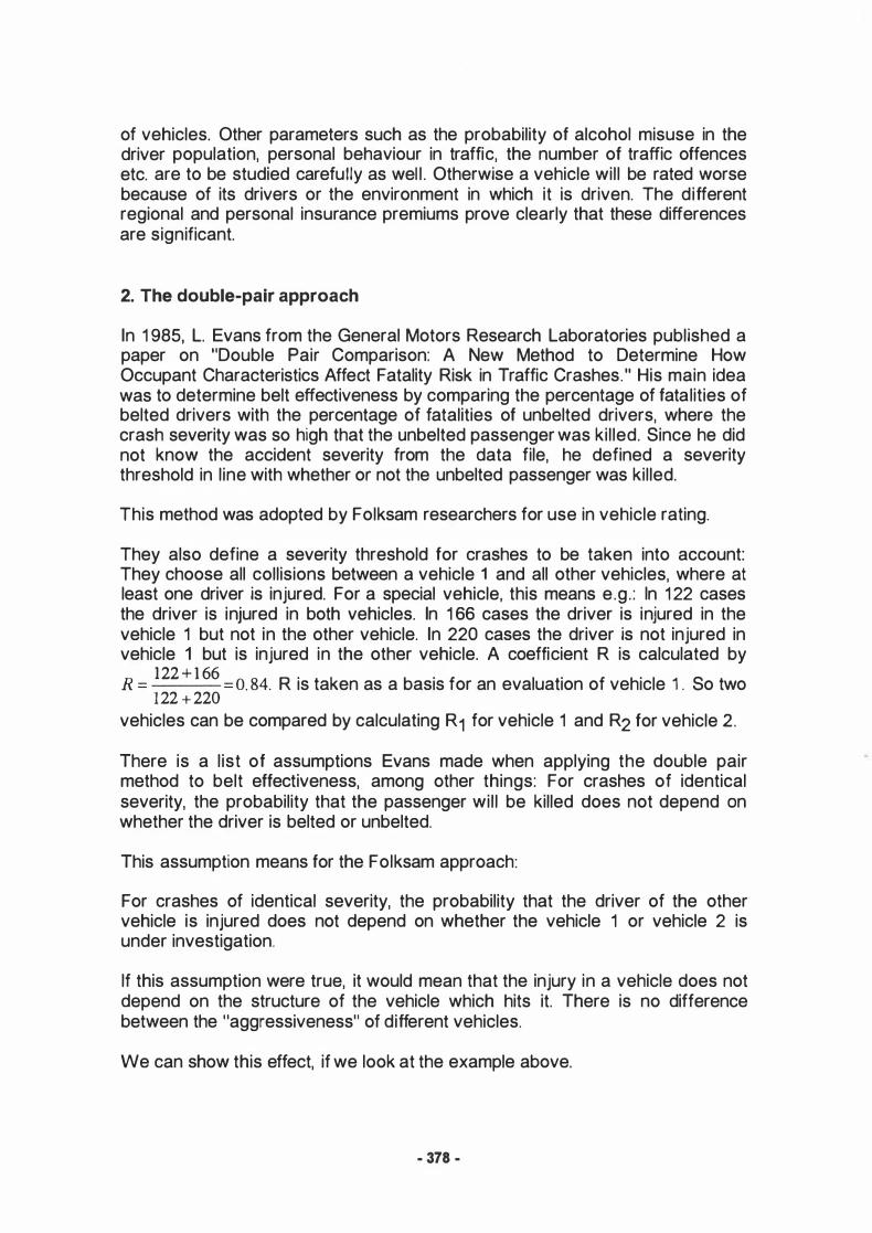
Table 5 l ists some of them. The Folksam procedure was already discussed as an application of the double-pair approach in chapter 2. The MRSC, the mean risk of serious consequences, is very simply computed from insurance data. lt is the arithmetical average of all serious consequences ( death or disablement). The computation is not very clear. Unclear is, how belted and unbelted occupants are treated. Unclear is also, what the basis of MRSC is. lt seems to be the mean value for all injured occupants. So it is somewhat like the conditional probabil ity of serious consequences, when an injury occurred. Z = R * MRSC is the risk of serious consequences for the vehicle under review, in the extend that R is proportional to the risk of injury. The parameter Z is a mixture of different datasets, and, of course, no better than R, from which it is derived. So all the discussions of R in chapter 2 hold also for Z. When Folksam publishes its results, a more precise description of the datasets and of the data subsets used for the computation of special figures would be helpful. Table 5 shows that the results for R, and thus also for Z are negative correlated to the vehicle mass. Folksam-R shows the highest negative correlation to mass.

Vehicle Ratings

Rating Approach Country Source

Folksam R Sweden Police data MRSC lnsurance data Z=R*MRSC Mixture of both

M.O.T. R (injured) Gr. Britain Police data R ( severely inj.) Police data

Oulu R Finland Pol ice/lnsurance lnj. vs. accidents lnsurance data lnj.vs.mileage lnsurance data

HLDI lnj. vs. veh. -month U.S.A. lnsurance data llHS Fatalities vs. U.S.A. FARS (police data)

vehicle-month Actual vs.predicted FARS (police data)

Column "Veh" Number of vehicles rated R various applications of the double-pair approach MRSC mean risk of serious consequences

Table 5: Different vehicle ratings.

- 382 -

Veh. Corr.to mass

58 -0.91 58 -0.05 58 -0.72 9 1 -0.88 91 -0.69 62 -0.83 62 -0.72 62 -0.80 1 70 -0.79 1 03 -0.27

1 03 0 . 16

M.O.T., the Ministry of Transportation of the United Kingdom, computes a R­value similar to Folksam. The main difference is the fact that the M.O.T. value is a value between O and 1 , because M.O.T. computes the ratio of the number of injured drivers in vehicle 1 , the vehicle under review, and as denominator the number of all accidents with involvement of vehicle 1 , and at least one injured driver. But in principal the M.O.T. approach is also a double-pair approach like Folksam, and the arguments of chapter 2 hold.

Again the correlation to mass is high, but it decreases a little, when comparing the R-value derived from severely injured. This observation can also be made when comparing HLDI and l lHS (Table 5).

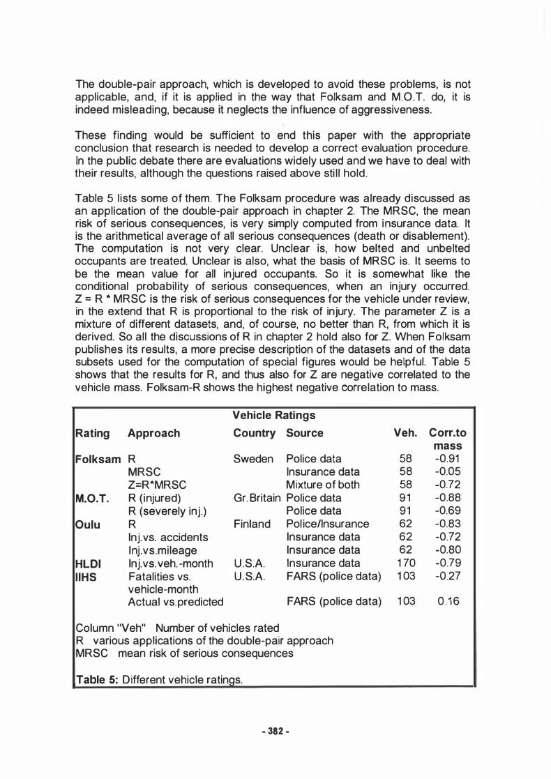
The University of Oulu presented a very interesting paper, producing an R value comparable to Folksam. But in addition, they also evaluate the vehicles by the number of injuries applied to the number of accidents or the mileage. So a comparison between these figures is possible. Table 6 lists the best vehicles by "accidents per 1 00 insurance-years" and "accidents per 1 million kilometres". Only the best vehicles in this sense are listed. These figures should describe the ability of crash avoidance of a vehicle.

The best vehicle should be a vehicle with a highly-sophisticated running gear. Per 1 00 insurance-years the best vehicles are VW Beetle and Wartburg, per 1 mil l ion km the best vehicles are the MB 1 24 and MB 1 23. The VW Beetle is the vehicle with the smallest mileage (9095 km/year), MB 1 24, MB 1 23, and Wartburg are the three vehicles with the smallest percentage of young automobile owners in the list. While there is an average of 1 2,0 % of automobile owners between the ages of 1 8 - 24 years in Finland, in the case of MB 1 24 there are 0,0 %, in the case of MB 1 23 2,9 %, and in the case of Wartburg 3,6 % of these, the youngest and most accident-endangered car owners. So "accidents per 1 mill ion kilometres" detected the vehicles with the smallest percentage of young drivers. lt has to be proven, whether and how far the "active safety" figure "accidents per 1 million km" reflects the active safety of the vehicle and not only the driving abil ity of the ownership of the specific vehicle.

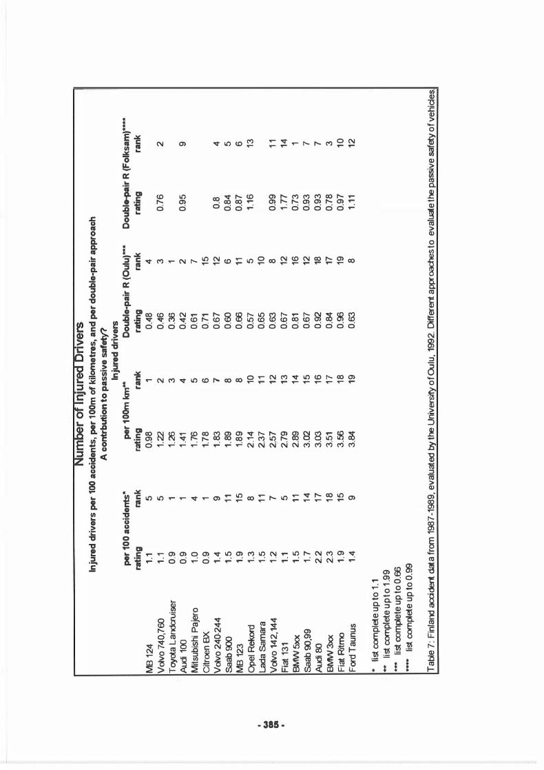
A good figure to describe passive safety might be the number of injured drivers per 1 00 accidents. Active safety determines whether an accident occurs or not. Passive safety determines the injury which is suffered in a specific accident. The list given in table 7 is complete for every column up to a certain level, so that the best vehicles are given for every column. The rank is given for every column. No statistical evaluation of the different rankings of the list is necessary. The position of a vehicle depends to an large extend on the method by which the vehicle is ranked. A customer who wants to buy the best vehicle has to buy as many vehicles as rankings exist. In ice-dance you also have a lot of different rankings by different referees. They add the rankings together to choose the champion. In an area which deals with welfare of people, we should be more careful . We should discuss the reasons for the differences in the rankings. We should answer the question, what the different rankings are measuring. The differences prove at least that the ratings are not measuring

- 383 -

"the safety of the vehicle" but something eise. This might be a partial aspect of "the safety", but this might also be an exposure effect of environment or driver. And in some cases it might be just the wrong approach.

N umber of Accidents

Accidents per 1 00 insurance years and 1 m of kilometres

Accidents per 1 00 insurance years* 1 m km**

rating VW Beetle 3 Wartburg 3.3 N issan Sunny 86- 3.4 N issan Sunny B1 1 82- 3.4 Nissan Micra 3.5 Saab 95,96 3.6 Skoda 3.6 Opel Corsa 3.6 Toyota Corolla 83-86 3.9 VW Golf/Jetta 4.4 Volvo 740,760 5.3 Opel Ascona 4.4 MB 1 24 5 MB 1 23 4.2 MB 1 1 4 , 1 1 5 4.5 * List complete for rating < 4 ** List complete for rating < 2

rank 1 2 3 3 5 6 6 6 9

1 1 1 5 1 1 1 4 1 0 1 3

rating 3.3 2.5 1 .6 1 .6 2.3 2.7 2.9 1 .9 1 .8 1 .9 1 .6 1 .9 1 .3 1 .5 1 .9

rank 1 5 1 2 3 3

1 1 1 3 1 4 7 6 7 3 7 1 2 7

Table 6: Finland accident data from 1 987-1 989, evaluated by the University o1 Oulu, 1 992. The number of accidents, applied to 1 00 insurance years and 1 mil l ion ki lometres, should evaluate the active safety of vehicles. The result looks rather strange.

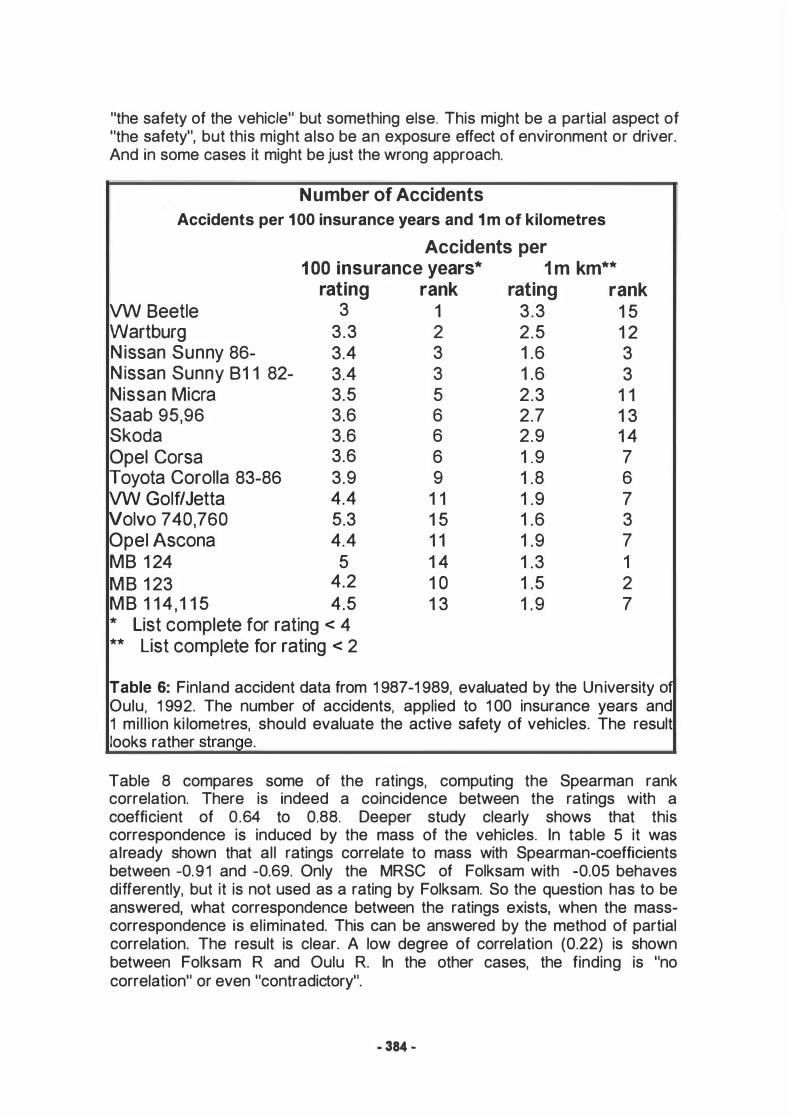
Table 8 compares some of the ratings, computing the Spearman rank correlation. There is indeed a coincidence between the ratings with a coefficient of 0.64 to 0.88. Deeper study clearly shows that this correspondence is induced by the mass of the vehicles. In table 5 it was already shown that all ratings correlate to mass with Spearman-coefficients between -0.91 and -0.69. Only the MRSC of Folksam with -0.05 behaves differently, but it is not used as a rating by Folksam. So the question has to be answered, what correspondence between the ratings exists, when the mass­correspondence is eliminated. This can be answered by the method of partial correlation. The result is clear. A low degree of correlation (0.22) is shown between Folksam R and Oulu R. In the other cases, the finding is "no correlation" or even "contradictory".

- 384 -

• w

Ot

OI

Numbe

r of l

njured

Drivers

lnju

red

dri

ve

rs pe

r 100

acc

ide

nts

, pe

r 10

0m of

kilom

etre

s, a

nd

per

do

ub

le-p

air

ap

pro

ac

h

per

100

ac

cid

ents

*

ratin

g

MB

124

1.1

Vol

vo 7

40,7

60

1.1

Toy

ota

Landau

iser

0.9

Aud

i 100

0.

9 M

itsub

ishi

Paj

ero

1.0

Citr

oen

BX

0.9

Vol

vo 2

40-2

44

1.4

Sa

ab90

0 1.

5

MB

123

1.9

Op

el R

ekor

d 1.

3

IL..ada

Sam

ara

1.5

Vol

vo 1

42, 1

44

1.2

Fiat

131

1.

1 BWr./'J

5xx

1.5

Sa

ab90

,99

1.7

Au

di80

2.

2 BW

W'J3xx

2.3

Fiat

Ritmo

1.

9

Ford

Tau

nus

1.4

*

list com

plet

e up

to 1

.1

**

list com

plet

e up

to 1.

99

***

list co

mpl

ete

up to

0.66

-

. list

compl

ete

up to

0.99

ran

k

5 5 1 1 4 1 9 11

15

8 11

7 5 11

14

17

18

15

9

A c

ont

rbut

ion

to

pa

ss

ive

safety?

lnju

red

dri

ve

rs

per

1 OOm

km**

Do

ub

le-p

air

R (

Ou

lu)**

* D

ou

ble-pa

ir R

(F

olk

sa

m)*

***

ratin

g

ran

k

ratin

g

ran

k

ratin

g

ran

k

0.98

1

0.48

4

1.22

2

0.46

3

0.76

2

1.26

3

0.36

1.

41

4 0.

42

2 0.

95

9 1.

76

5 0.

61

7 1.7

8 6

0.71

15

1.

83

7 0.

67

12

0.8

4 1.

89

8 0.

60

6 0.

84

5 1.8

9 8

0.66

11

0.

87

6 2

.14

10

0.

57

5 1.

16

13

2.37

11

0.

65

10

2.57

12

0.

63

8 0.

99

11

2.79

13

0.

67

12

1.77

14

2.

89

14

0.81

16

0.

73

1 3.

02

15

0.67

12

0.

93

7 3.

03

16

0.92

18

0.

93

7 3.

51

17

0.84

17

0.

78

3 3.

56

18

0.96

19

0.

97

10

3.84

19

0.

63

8 1.

11

12

Tabl

e 7:

Fin

land

accident

data

from

198

7-198

9, e

valu

ated

by the

Uni

versity o

f Oulu

, 199

2. Di

ffer

ent a

pproaches

to e

valuat

e the

passi

ve sa

fety o

f veh

ides

.

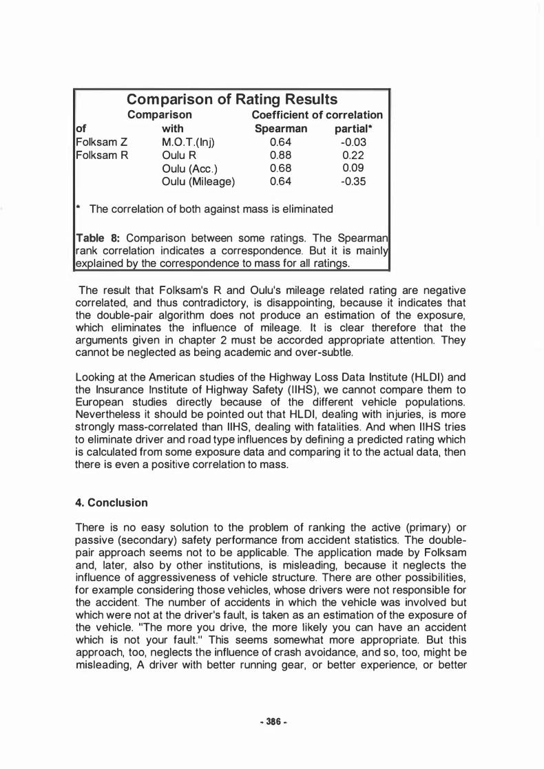
Comparison of Rating Results Comparison Coefficient of correlation

of Folksam Z Folksam R

with Spearman partial*

M.0.T.( lnj) 0.64 -0.03 Oulu R 0.88 0.22 Oulu (Ace.) 0.68 0.09 Oulu (Mi leage) 0.64 -0.35

* The correlation of both against mass is eliminated

Table 8: Comparison between some ratings. The Spearman rank correlation indicates a correspondence. But it is mainly explained by the correspondence to mass for all ratinQs.

The result that Folksam's R and Oulu's mileage related rating are negative correlated, and thus contradictory, is disappointing, because it indicates that the double-pair algorithm does not produce an estimation of the exposure, which eliminates the influence of mileage. lt is clear therefore that the arguments given in chapter 2 must be accorded appropriate attention. They cannot be neglected as being.academic and over-subtle.

Looking at the American studies of the Highway Loss Data Institute (HLDI) and the lnsurance Institute of Highway Safety ( l lHS), we cannot compare them to European studies directly because of the different vehicle populations. Nevertheless it should be pointed out that HLDI, dealing with injuries, is more strongly mass-correlated than l lHS, dealing with fatalities. And when l lHS tries to eliminate driver and road type influences by defining a predicted rating which is calculated from some exposure data and comparing it to the actual data, then there is even a positive correlation to mass.

4. Conclusion

There is no easy solution to the problem of ranking the active (primary) or passive (secondary) safety performance from accident statistics. The double­pair approach seems not to be applicable. The appl ication made by Folksam and, later, also by other institutions, is misleading, because it neglects the influence of aggressiveness of vehicle structure. There are other possibil ities, for example considering those vehicles, whose drivers were not responsible for the accident. The number of accidents in which the vehicle was involved but which were not at the driver's fault, is taken as an estimation of the exposure of the vehicle. "The more you drive, the more l ikely you can have an accident which is not your fault." This seems somewhat more appropriate. But this approach, too, neglects the influence of crash avoidance, and so, too, might be misleading, A driver with better running gear, or better experience, or better

- 386 .

accident-avoidance training, will be assumed to be somebody, who does not drive so much. Same attempts to use this procedure have clearly failed entirely.

A method of ranking the safety performance of vehicles, presupposes a thorough knowledge of the exposure of the vehicle to environment and driver.

Environment means primarily the mileage covered on the different road types. However, other aspects may also be relevant. The age- and sex-breakdown of the driver population should be known. But it is conceivable that the social class and environment of a person, and the possibility of alcohol abuse, will also influence the risk of an accident and the accident severity.

As a conclusion we can state that a rating of vehicles by accident data additionally requires the intensive study of exposure data. Otherwise it cannot be clearly ascertained, whether the "rating" figure as computed rates

the environment, in which the vehicle is driven, or the driver who drives the vehicle with greater or lesser care, or the vehicle itself, or something eise, or a combination of all these parameters.

No rating that is published today is clear on this point. The discrepancies in the ratings which are available today show that this work has to be done. An easy solution does not exist. There is as yet no such thing as "the" definitive accident performance rating. lt is the opinion of the author that without differentiated exposure data, it is not possible to rate vehicles. At the very least, exposure data are necessary to prove that a rating really rates the vehicle, and not something eise.

5. References

1 F olksam Car Model Safety Rating 1 991 /92, Stockholm 1 992

2 How Safe is Your Car? Result of 25 Years' Research of Actual Car Accidents. Folksam. Stockholm 1 994

3 The Ministry of Transportation Statistics Report. Cars: Make and Model : . lnjury Accident and Casuality Rates. Great Britain: 1 991 . London 1 993

4 Buying a Car? Choose Safety. Leaflet of the Ministry of Transportation. London 1 993

5 Ernvall, T. and Pirtala, P. The Effect of Drivers Age And Experience And Car Model on Accident Risk. Road and Transport Laboratory. University of Oulu, 1 992

6 lnsurance lnjury Report 190-1 . Highway Lass Data Institute. Arlington, Virginia, 1 991

- 387 -

7 Technical Appendix. Highway Loss Data Institute. Arlington, Virginia, 1 991

8 lnsurance Institute for Highway Safety Status Report, Special Report: Occupant Death Rates, 1 984-88 Model Cars (Vol. 26, No. 4). Arlington, Virginia, 1 991

9 Computing Fatality Rates By Make and Series of Passenger Cars: 1 984-88 Models. lnsurance Institute for Highway Safety, Arlington, Virginia, 1 991

1 0 Cameron, M. , Mach, T., and Neiger, D. Vehicle Crashworthiness Ratings: Victoria 1 983-90 and NSW 1 989-90 Crashes. Summary Report. Monash University Accident Research Centre, Australia, 1 992

1 1 How does your car rate in a crash? Driver Protection Ratings of 1 982-90 Cars, Station Wagons, Passenger Vans and Four Wheel Drives. Leaflet of the Monash University Accident Research Centre, Australia, 1 992

1 2 Evans, L. Double Pair Comparison: A New Method To Determine How Occupant Characteristics Affect Fatality Risk In Traffic Crashes. General Motors Research Laboratories, Warren, Michigan, 1 985

· 388 .