Embed Size (px)
Citation preview
ACES II Release 2.5.0
User Manual
DRAFT COPY
Quantum Theory Project
P.O. Box 118435
University of Florida
Gainesville, FL 32611
January 29, 2006
Contents
Contents 1
1 Authors 7
1.1 Official ACES II citation . . . . . . . . . . . . . . . . . . . . . . . . . . . . 7
1.2 Specific authors . . . . . . . . . . . . . . . . . . . . . . . . . . . . . . . . . . 7
2 Preface 9
3 Introduction 10
3.1 Overview of capabilities of ACES II . . . . . . . . . . . . . . . . . . . . . . 11
4 Quickstart Guide 14
5 Program Structure 15
5.1 aces2 and p aces2 . . . . . . . . . . . . . . . . . . . . . . . . . . . . . . . 15
5.2 joda . . . . . . . . . . . . . . . . . . . . . . . . . . . . . . . . . . . . . . . . 15
5.3 mopac . . . . . . . . . . . . . . . . . . . . . . . . . . . . . . . . . . . . . . . 15
5.4 vmol . . . . . . . . . . . . . . . . . . . . . . . . . . . . . . . . . . . . . . . 15
5.5 vmol2ja . . . . . . . . . . . . . . . . . . . . . . . . . . . . . . . . . . . . . 16
5.6 vprops . . . . . . . . . . . . . . . . . . . . . . . . . . . . . . . . . . . . . . 16
5.7 nddo . . . . . . . . . . . . . . . . . . . . . . . . . . . . . . . . . . . . . . . 16
5.8 vscf, p vscf, vscf ks, intgrt, and intpack . . . . . . . . . . . . . . . . 16
5.9 dirmp2 and p dirmp2 . . . . . . . . . . . . . . . . . . . . . . . . . . . . . . 16
5.10 vtran . . . . . . . . . . . . . . . . . . . . . . . . . . . . . . . . . . . . . . . 16
5.11 tdhf . . . . . . . . . . . . . . . . . . . . . . . . . . . . . . . . . . . . . . . . 16
5.12 intprc . . . . . . . . . . . . . . . . . . . . . . . . . . . . . . . . . . . . . . 17
5.13 vcc, vcc5t, and vcc5q . . . . . . . . . . . . . . . . . . . . . . . . . . . . . 17
5.14 mrcc . . . . . . . . . . . . . . . . . . . . . . . . . . . . . . . . . . . . . . . 17
5.15 fno . . . . . . . . . . . . . . . . . . . . . . . . . . . . . . . . . . . . . . . . 17
5.16 lambda . . . . . . . . . . . . . . . . . . . . . . . . . . . . . . . . . . . . . . 17
5.17 vea and vee . . . . . . . . . . . . . . . . . . . . . . . . . . . . . . . . . . . 17
5.18 vcceh . . . . . . . . . . . . . . . . . . . . . . . . . . . . . . . . . . . . . . . 17
5.19 dens . . . . . . . . . . . . . . . . . . . . . . . . . . . . . . . . . . . . . . . . 17
5.20 props . . . . . . . . . . . . . . . . . . . . . . . . . . . . . . . . . . . . . . . 18
5.21 anti . . . . . . . . . . . . . . . . . . . . . . . . . . . . . . . . . . . . . . . . 18
5.22 bcktrn . . . . . . . . . . . . . . . . . . . . . . . . . . . . . . . . . . . . . . 18
5.23 vdint, vksdint, scfgrd, and p scfgrd . . . . . . . . . . . . . . . . . . . 18
1
5.24 cphf . . . . . . . . . . . . . . . . . . . . . . . . . . . . . . . . . . . . . . . . 18
5.25 nmr . . . . . . . . . . . . . . . . . . . . . . . . . . . . . . . . . . . . . . . . 18
5.26 asv . . . . . . . . . . . . . . . . . . . . . . . . . . . . . . . . . . . . . . . . 19
5.27 a2proc . . . . . . . . . . . . . . . . . . . . . . . . . . . . . . . . . . . . . . 19
5.27.1 clrdirty . . . . . . . . . . . . . . . . . . . . . . . . . . . . . . . . . 19
5.27.2 mem . . . . . . . . . . . . . . . . . . . . . . . . . . . . . . . . . . . . 19
5.27.3 zerorec . . . . . . . . . . . . . . . . . . . . . . . . . . . . . . . . . 20
5.27.4 rmfiles . . . . . . . . . . . . . . . . . . . . . . . . . . . . . . . . . . 20
5.27.5 parfd . . . . . . . . . . . . . . . . . . . . . . . . . . . . . . . . . . . 20
5.27.6 molden and hyperchem . . . . . . . . . . . . . . . . . . . . . . . . 20
5.27.7 jasum and iosum . . . . . . . . . . . . . . . . . . . . . . . . . . . . 20
5.27.8 jarec . . . . . . . . . . . . . . . . . . . . . . . . . . . . . . . . . . . 20
5.27.9 xyz . . . . . . . . . . . . . . . . . . . . . . . . . . . . . . . . . . . . 21
5.27.10test . . . . . . . . . . . . . . . . . . . . . . . . . . . . . . . . . . . . 21
5.28 gemini . . . . . . . . . . . . . . . . . . . . . . . . . . . . . . . . . . . . . . . 21
6 File Structure 22
6.1 ZMAT . . . . . . . . . . . . . . . . . . . . . . . . . . . . . . . . . . . . . . . . 22
6.2 GENBAS/ZMAT.BAS . . . . . . . . . . . . . . . . . . . . . . . . . . . . . . . . . 22
6.3 ECPDATA . . . . . . . . . . . . . . . . . . . . . . . . . . . . . . . . . . . . . . 22
6.4 GUESS . . . . . . . . . . . . . . . . . . . . . . . . . . . . . . . . . . . . . . . 22
6.5 NEWMOS/OLDMOS . . . . . . . . . . . . . . . . . . . . . . . . . . . . . . . . . . 22
6.6 AOBASMOS/OLDAOMOS . . . . . . . . . . . . . . . . . . . . . . . . . . . . . . . 22
6.7 FCMINT, FCM, FCMSCR, and FCMFINAL . . . . . . . . . . . . . . . . . . . . . 23
6.8 frequency . . . . . . . . . . . . . . . . . . . . . . . . . . . . . . . . . . . . . 23
6.9 ISOMASS . . . . . . . . . . . . . . . . . . . . . . . . . . . . . . . . . . . . . . 23
6.10 System files . . . . . . . . . . . . . . . . . . . . . . . . . . . . . . . . . . . . 23
6.10.1 JOBARC, JAINDX . . . . . . . . . . . . . . . . . . . . . . . . . . . . . 23
6.10.2 MOINTS, GAMLAM, MOABCD, DERINT, DERGAM . . . . . . . . . . . . . 23
6.10.3 MOL, IIII, IIJJ, IJIJ, IJKL . . . . . . . . . . . . . . . . . . . . . 23
6.10.4 OPTARC/OPTARCBK . . . . . . . . . . . . . . . . . . . . . . . . . . . . . 24
6.10.5 DIPOL, DIPDER, POLAR, POLDER . . . . . . . . . . . . . . . . . . . . 24
6.10.6 GRD . . . . . . . . . . . . . . . . . . . . . . . . . . . . . . . . . . . . . 24
6.10.7 HF2, HF2AA, HF2AB, HF2BB . . . . . . . . . . . . . . . . . . . . . . . 24
6.10.8 IUHF . . . . . . . . . . . . . . . . . . . . . . . . . . . . . . . . . . . . 24
6.10.9 TGUESS, LGUESS . . . . . . . . . . . . . . . . . . . . . . . . . . . . . 24
6.10.10VPOUT . . . . . . . . . . . . . . . . . . . . . . . . . . . . . . . . . . . 24
6.10.11GAMESS.LOG, MP2.LOG, DIRGRD.LOG . . . . . . . . . . . . . . . . . . 24
2
6.10.12OUT.000, DUMP.000, 1ELGRAD.000 . . . . . . . . . . . . . . . . . . . 25
7 File Formats 26
7.1 ZMAT . . . . . . . . . . . . . . . . . . . . . . . . . . . . . . . . . . . . . . . . 26
7.1.1 File anatomy . . . . . . . . . . . . . . . . . . . . . . . . . . . . . . . 26
7.1.2 Examples . . . . . . . . . . . . . . . . . . . . . . . . . . . . . . . . . 27
7.1.3 File directives . . . . . . . . . . . . . . . . . . . . . . . . . . . . . . . 28
7.1.4 Molecular orientation . . . . . . . . . . . . . . . . . . . . . . . . . . . 29
7.1.5 Dummy and ghost atoms . . . . . . . . . . . . . . . . . . . . . . . . . 30
7.1.6 Cartesian coordinates . . . . . . . . . . . . . . . . . . . . . . . . . . . 30
7.1.7 Internal coordinates . . . . . . . . . . . . . . . . . . . . . . . . . . . . 31
7.1.8 Z matrix analyzer . . . . . . . . . . . . . . . . . . . . . . . . . . . . . 33
7.1.9 *ACES2 namelist . . . . . . . . . . . . . . . . . . . . . . . . . . . . . . 34
7.1.10 Line-item basis/ECP definitions . . . . . . . . . . . . . . . . . . . . . 37
7.2 GENBAS/ZMAT.BAS . . . . . . . . . . . . . . . . . . . . . . . . . . . . . . . . . 37
7.3 ECPDATA . . . . . . . . . . . . . . . . . . . . . . . . . . . . . . . . . . . . . . 39
7.4 GUESS . . . . . . . . . . . . . . . . . . . . . . . . . . . . . . . . . . . . . . . 40
8 Keywords 42
8.1 *ACES2 namelist . . . . . . . . . . . . . . . . . . . . . . . . . . . . . . . . . . 42
8.1.1 System: general . . . . . . . . . . . . . . . . . . . . . . . . . . . . . . 43
8.1.2 System: molecular control . . . . . . . . . . . . . . . . . . . . . . . . 44
8.1.3 System: debug . . . . . . . . . . . . . . . . . . . . . . . . . . . . . . 45
8.1.4 I/O subsystem . . . . . . . . . . . . . . . . . . . . . . . . . . . . . . 45
8.1.5 Chemical system . . . . . . . . . . . . . . . . . . . . . . . . . . . . . 46
8.1.6 Basis set . . . . . . . . . . . . . . . . . . . . . . . . . . . . . . . . . . 46
8.1.7 Integrals . . . . . . . . . . . . . . . . . . . . . . . . . . . . . . . . . . 47
8.1.8 Reference . . . . . . . . . . . . . . . . . . . . . . . . . . . . . . . . . 48
8.1.9 SCF: general . . . . . . . . . . . . . . . . . . . . . . . . . . . . . . . 49
8.1.10 SCF: orbital control . . . . . . . . . . . . . . . . . . . . . . . . . . . 49
8.1.11 SCF: iteration control . . . . . . . . . . . . . . . . . . . . . . . . . . 51
8.1.12 SCF reference adjustments . . . . . . . . . . . . . . . . . . . . . . . . 52
8.1.13 Post-SCF file options . . . . . . . . . . . . . . . . . . . . . . . . . . . 55
8.1.14 Post-SCF calculations . . . . . . . . . . . . . . . . . . . . . . . . . . 57
8.1.15 Excited states: general . . . . . . . . . . . . . . . . . . . . . . . . . . 58
8.1.16 Excited states: properties . . . . . . . . . . . . . . . . . . . . . . . . 59
8.1.17 Excited states: affinities . . . . . . . . . . . . . . . . . . . . . . . . . 60
8.1.18 Excited states: electronic (absorption) . . . . . . . . . . . . . . . . . 61
3
8.1.19 Excited states: ionizations . . . . . . . . . . . . . . . . . . . . . . . . 62
8.1.20 Excited states: gradients . . . . . . . . . . . . . . . . . . . . . . . . . 63
8.1.21 Properties . . . . . . . . . . . . . . . . . . . . . . . . . . . . . . . . . 64
8.1.22 Geometry optimization: general . . . . . . . . . . . . . . . . . . . . . 66
8.1.23 Geometry optimization: stepping algorithm . . . . . . . . . . . . . . 66
8.1.24 Geometry optimization: iteration control . . . . . . . . . . . . . . . . 67
8.1.25 Geometry optimization: integral derivatives . . . . . . . . . . . . . . 68
8.1.26 Frequencies and other 2nd-order properties . . . . . . . . . . . . . . . 68
8.1.27 Finite displacements . . . . . . . . . . . . . . . . . . . . . . . . . . . 68
8.1.28 External interfaces . . . . . . . . . . . . . . . . . . . . . . . . . . . . 69
9 Examples 70
9.1 Single-point calculations . . . . . . . . . . . . . . . . . . . . . . . . . . . . . 70
9.1.1 RHF CCSD(T) energy . . . . . . . . . . . . . . . . . . . . . . . . . . 70
9.1.2 UHF CCSD(T) energy . . . . . . . . . . . . . . . . . . . . . . . . . . 70
9.1.3 ROHF CCSD(T) energy . . . . . . . . . . . . . . . . . . . . . . . . . 71
9.1.4 QRHF CCSD(T) energy . . . . . . . . . . . . . . . . . . . . . . . . . 71
9.1.5 Effective core potentials . . . . . . . . . . . . . . . . . . . . . . . . . 72
9.1.6 Initial guessing with OLDMOS . . . . . . . . . . . . . . . . . . . . . . . 72
9.1.7 Initial guessing with OLDAOMOS . . . . . . . . . . . . . . . . . . . . . . 73
9.1.8 Improving SCF convergence . . . . . . . . . . . . . . . . . . . . . . . 74
9.1.9 Hartree-Fock stability analysis . . . . . . . . . . . . . . . . . . . . . . 75
9.1.10 Time-dependent Hartree-Fock . . . . . . . . . . . . . . . . . . . . . . 77
9.1.11 EOM-CCSD excitation energy . . . . . . . . . . . . . . . . . . . . . . 79
9.1.12 EOM-CCSD electron attachment energy . . . . . . . . . . . . . . . . 79
9.1.13 NMR chemical shifts . . . . . . . . . . . . . . . . . . . . . . . . . . . 81
9.2 Geometry optimizations . . . . . . . . . . . . . . . . . . . . . . . . . . . . . 85
9.2.1 Full optimization of internal coordinates . . . . . . . . . . . . . . . . 85
9.2.2 Partial optimization of internal coordinates . . . . . . . . . . . . . . . 85
9.2.3 Full optimization of Cartesian coordinates . . . . . . . . . . . . . . . 86
9.2.4 Transition state search . . . . . . . . . . . . . . . . . . . . . . . . . . 87
9.2.5 Restarting an optimization (or frequency) calculation . . . . . . . . . 87
9.2.6 Initializing the Hessian with FCMINT in a geometry search . . . . . . . 88
9.3 Frequency calculations . . . . . . . . . . . . . . . . . . . . . . . . . . . . . . 89
9.3.1 Numerical frequencies from analytical gradients . . . . . . . . . . . . 89
9.3.2 Numerical frequencies from energies . . . . . . . . . . . . . . . . . . . 90
9.3.3 Isotopic shift . . . . . . . . . . . . . . . . . . . . . . . . . . . . . . . 90
4
10 Parallelization 92
10.1 Overview . . . . . . . . . . . . . . . . . . . . . . . . . . . . . . . . . . . . . . 92
10.2 Running xgemini . . . . . . . . . . . . . . . . . . . . . . . . . . . . . . . . . 93
10.2.1 Local scratch directories . . . . . . . . . . . . . . . . . . . . . . . . . 93
10.2.2 Shared scratch directories . . . . . . . . . . . . . . . . . . . . . . . . 94
10.2.3 Command-line flags and pattern macros . . . . . . . . . . . . . . . . 94
10.3 Examples . . . . . . . . . . . . . . . . . . . . . . . . . . . . . . . . . . . . . 96
10.3.1 Parallel finite differences with MPI (automatic) . . . . . . . . . . . . 96
10.3.2 Parallel finite differences with scripts (manual) . . . . . . . . . . . . . 97
10.3.3 SCF geometry optimizations . . . . . . . . . . . . . . . . . . . . . . . 99
11 Troubleshooting 100
11.1 Common mistakes . . . . . . . . . . . . . . . . . . . . . . . . . . . . . . . . . 100
11.2 Basic program restrictions . . . . . . . . . . . . . . . . . . . . . . . . . . . . 101
11.3 Suggestions for reducing resources . . . . . . . . . . . . . . . . . . . . . . . . 101
12 References 102
12.1 Many-body perturbation theory (MBPT) . . . . . . . . . . . . . . . . . . . . 102
12.2 Coupled-cluster (CC) theory . . . . . . . . . . . . . . . . . . . . . . . . . . . 103
12.3 Analytical gradients for MBPT/CC methods . . . . . . . . . . . . . . . . . . 104
12.4 Analytical second derivatives for MBPT/CC methods . . . . . . . . . . . . . 106
12.5 NMR chemical shift calculations . . . . . . . . . . . . . . . . . . . . . . . . . 106
12.6 Methods for calculating excitation energies . . . . . . . . . . . . . . . . . . . 106
12.7 Methods for calculating electron attachment energies . . . . . . . . . . . . . 107
12.8 Time-dependent Hartree-Fock methods . . . . . . . . . . . . . . . . . . . . . 107
12.9 HF-DFT method . . . . . . . . . . . . . . . . . . . . . . . . . . . . . . . . . 107
12.10Basis sets . . . . . . . . . . . . . . . . . . . . . . . . . . . . . . . . . . . . . 107
12.11Integral packages . . . . . . . . . . . . . . . . . . . . . . . . . . . . . . . . . 110
A Other Keywords 111
A.1 Experimental, obsolete, and unused . . . . . . . . . . . . . . . . . . . . . . . 111
A.2 Kohn-Sham DFT namelists . . . . . . . . . . . . . . . . . . . . . . . . . . . 112
A.2.1 *VSCF . . . . . . . . . . . . . . . . . . . . . . . . . . . . . . . . . . . 112
A.2.2 *INTGRT . . . . . . . . . . . . . . . . . . . . . . . . . . . . . . . . . 112
A.3 mrcc namelists . . . . . . . . . . . . . . . . . . . . . . . . . . . . . . . . . . 114
A.3.1 *mrcc gen, *true mrcc, *cse . . . . . . . . . . . . . . . . . . . . . . . 114
A.3.2 *EE EOM, *EE TDA, *EE STEOM . . . . . . . . . . . . . . . . . . 114
A.3.3 *IP EOM, *IP CI, *DIP EOM, *DIP TDA, *DIP STEOM . . . . . . 114
5
A.3.4 *EA EOM, *EA CI, *DEA EOM, *DEA TDA, *DEA STEOM . . . 114
A.3.5 *ACT EA EOM . . . . . . . . . . . . . . . . . . . . . . . . . . . . . . 114
B Standard Basis Sets and ECPs 115
B.1 Basis sets in GENBAS . . . . . . . . . . . . . . . . . . . . . . . . . . . . . . . 115
B.2 ECP sets in ECPDATA . . . . . . . . . . . . . . . . . . . . . . . . . . . . . . . 131
C Queue Scripts 132
C.1 ACES II script body . . . . . . . . . . . . . . . . . . . . . . . . . . . . . . . 132
C.2 LoadLeveler . . . . . . . . . . . . . . . . . . . . . . . . . . . . . . . . . . . . 132
C.3 LSF . . . . . . . . . . . . . . . . . . . . . . . . . . . . . . . . . . . . . . . . 132
C.4 GridEngine . . . . . . . . . . . . . . . . . . . . . . . . . . . . . . . . . . . . 132
Index 134
6
1 Authors
1.1 Official ACES II citation
The users of ACES II must give the following citation:
ACES II is a program product of the Quantum Theory Project, University
of Florida. Authors: J.F. Stanton, J. Gauss, S.A. Perera, J.D. Watts, A.D.
Yau, M. Nooijen, N. Oliphant, P.G. Szalay, W.J. Lauderdale, S.R. Gwaltney,
S. Beck, A. Balkova, D.E. Bernholdt, K.K. Baeck, P. Rozyczko, H. Sekino, C.
Huber, J. Pittner, W. Cencek, D. Taylor, and R.J. Bartlett. Integral packages
included are VMOL (J. Almlof and P.R. Taylor); VPROPS (P. Taylor); ABA-
CUS (T. Helgaker, H.J. Aa. Jensen, P. Jørgensen, J. Olsen, and P.R. Taylor);
HONDO/GAMESS (M.W. Schmidt, K.K. Baldridge, J.A. Boatz, S.T. Elbert,
M.S. Gordon, J.J. Jensen, S. Koseki, N. Matsunaga, K.A. Nguyen, S. Su, T.L.
Windus, M. Dupuis, J.A. Montgomery).
The basis set distributed with the ACES II program system is obtained through Pacific
Northwest National Laboratory (PNNL) and any calculation that uses basis sets from this
catalog must give the following citation in addition to the ACES II citation.
Basis sets were obtained from the Extensible Computational Chemistry Envi-
ronment Basis Set Database, Version 1.0, as developed and distributed by the
Molecular Science Computing Facility, Environmental and Molecular Sciences
Laboratory which is part of the Pacific Northwest Laboratory, P.O. Box 999,
Richland, Washington 99352, USA, and funded by the U.S. Department of En-
ergy. The Pacific Northwest Laboratory is a multi-program laboratory operated
by Battelle Memorial Institute for the U.S. Department Energy under contract
DE-AC06-76RLO 1830. Contact Karen Schuchardt for further information.
1.2 Specific authors
• TD-CCSD energies. P.G. Szalay and A. Balkova.
• TD-CCSD analytical derivatives. P.G. Szalay.
• Dropped molecular orbitals in analytical derivative calculations for RHF, UHF, and
ROHF references. K.-K. Baeck.
• Equation-of-motion CCSD calculation of dynamic polarizabilities (including parti-
tioned scheme). J.F. Stanton, S.A. Perera, and M. Nooijen.
7

• Equation-of-motion CCSD calculation of NMR spin-spin coupling constants (including
partitioned scheme). S.A. Perera and M. Nooijen.
• Partitioned equation-of-motion CCSD calculations of excitation energies. S.R. Gwalt-
ney and M. Nooijen.
• Equation-of-motion CCSD gradient calculations for excited states. J.F. Stanton and
J. Gauss
8
2 Preface
This manual is maintained as a set of LATEX documents under CVS control along with the
ACES II source code. Every version of the code has an accompanying manual, and while
the user interface is relatively stable, it is not guaranteed that the manual of one version is
compatible with binary executables of a different version. Any errors in the manual should
be reported to [email protected]
The goal of this manual is to provide beginners and experts alike with enough information
to run any calculation that the software allows. A reference section is provided for further
reading on the theories and algorithms implemented in the program.
9
3 Introduction
ACES II is a set of programs that performs ab initio quantum chemistry calculations.
The package has a high degree of flexibility and supports many kinds of calculations at a
number of levels of theory. The major strength of the program system is using “many-body”
methods to treat electron correlation. These approaches, broadly categorized as many-body
perturbation theory (MBPT) and the coupled-cluster (CC) approximation, offer a reliable
treatment of correlation and have the attractive property of size-extensivity, which means
the energies scale properly with the size of the system. As a result of this property, MBPT
and CC methods are ideally suited for the study of chemical reactions. While ACES II can
perform Hartree-Fock Self-Consistent-Field (HF-SCF) and Kohn-Sham Density Functional
Theory (KS-DFT) calculations, the ACES II program system is not intended for large scale
HF-SCF or KS-DFT calculations.
Two important features of the ACES II program system are its effective use of molec-
ular symmetry, particularly in MBPT and CC calculations, and the sophisticated gradient
methods which are included in the program. Even if a few elements of symmetry are present
in a molecular system, differences in execution times required for calculations with symme-
try and without can be dramatic. The implementation of symmetry currently is limited to
D2h and its subgroups, and the expected speedup due to symmetry utilization will be on
the order of the square of the order of the computational point group for all steps except
integral and integral derivative generation and integral sorts, in which the speedup can be
no greater than the order of the group.
Gradient techniques are implemented for SCF and the following correlated levels of the-
ory: MBPT(2), MBPT(3), MBPT(4), CCD, QCISD, CCSD, QCISD(T), and CCSD(T) for
both restricted and unrestricted Hartree-Fock (RHF and UHF, respectively) reference func-
tions. In addition, for the MBPT(2), MBPT(3), CCSD, and CCSD(T) methods, gradients
are available for restricted open-shell Hartree-Fock (ROHF) reference functions. They are
also available for certain CCSD calculations based on quasi-restricted Hartree-Fock (QRHF)
reference functions, namely those for high-spin doublet cases and two-determinant CCSD
(TD-CCSD) calculations for open-shell singlet states, in which the open-shell orbitals have
different symmetries.
Efficient algorithms for geometry optimization and transition state searching have also
been included, and may be used at all levels of theory. The analytical gradients employed
during geometry optimizations and vibrational frequency calculations depend on their avail-
ability. When analytical gradients are not available, automated finite differencing proce-
dures can be used to compute the derivatives. Analytic second derivatives have been imple-
mented for SCF using RHF, UHF, and ROHF reference functions. In addition, analytically
evaluated NMR chemical shift tensors are available at the SCF and MBPT(2) levels using
10
gauge-including atomic orbitals (GIAOs) to ensure exact gauge-invariance. Other features
include the direct calculation of electronic excitation energies using the Tamm-Dancoff (or
configuration interaction singles) model (CIS), the random-phase approximation (RPA), the
equation-of-motion coupled-cluster approach (EOM-CC) and similarity transform-equation-
of-motion (STEOM), and molecular ionization potentials and electron affinities with EOM,
STEOM, and Fock-space coupled-cluster methods. Transition moments between ground
and excited states can be calculated for all of the methods, as well as selected excited state
properties. The excited state geometry optimization and frequency calculations employ the
analytical gradients capabilities available for the EOM and STEOM methods.
The programs collectively known as ACES II began development in early 1990, and the
first version of the code was written by J.F. Stanton, J. Gauss, J.D. Watts, W.J. Lauderdale,
and R.J. Bartlett. Program development is continuing, and the capabilities as well as the
contributors to the development of the ACES II program system are continually increas-
ing. At present, there are more than 30 member executables, each of which performs a
well-defined function and communicates with the rest of ACES II through stored files. The
ACES II program system has been interfaced with external programs such as MOLCAS and
GAMESS. The primary function of the MOLCAS and GAMESS interfaces is to provide in-
tegral and integral derivative programs that are more efficient and have direct capabilities to
complement the functionalities of the locally modified version of vmol, vprops, and vdint
programs. A complete replacement of these member executables is not yet feasible since the
specialized integrals such as Gauge-origin-independent (GIAO) integrals and NMR spin-spin
coupling operator integrals are only available in vmol, vprops, and vdint. ACES II can
also generate interfaces to graphical programs such as MOLDEN and gOpenMol, wave func-
tion analysis codes such as Natural Bond Orbital (NBO), and semi-emperical programs such
as HyperChem, NDDO, and MOPAC. The ACES II distribution comes with these capabil-
ities; however, ACES II developers are not responsible for distributing or maintaining the
external programs. Having independent licenses for external programs along with ACES II
will allow users to take full advantage of this functionality.
Since ACES II is the product of academic research group, and not a software company,
we are unable to guarantee that all results obtained with it are correct. Although we have
made great progress in removing serious errors from the codes, problems may still occur
and should be reported to [email protected]. Any suggestions for improving the input or
output, “wish-lists” for features, or other comments may also be sent to this address.
3.1 Overview of capabilities of ACES II
The general capabilities of ACES II to determine single point energies, analytical gra-
dients, and analytical hessians are as follows:
11
Single point energy calculations:
• Independent particle models include RHF, UHF, and ROHF.
• Correlation methods utilizing RHF and UHF reference determinants include MBPT(2),
MBPT(3), SDQ-MBPT(4), MBPT(4), CCD, CCSD, CCSD(T), CCSD+TQ∗(CCSD),
CCSD(TQ), CCSDT-1 CCSDT-2, CCSDT-3, QCISD, QCISD(T), QCISD(TQ), UCCS(4),
UCCSD(4), CID, and CISD.
• Correlation methods that can use ROHF reference determinants include MBPT(2),
CCSD, CCSDT, CCSD(T), CCSDT-1, CCSDT-2, and CCSDT-3.
• Correlation methods that can use QRHF or Brueckner orbital reference determinants
include CCSD, CCSDT, CCSD(T), CCSDT-1, CCSDT-2, and CCSDT-3.
• Two-determinant CCSD calculations for open-shell singlet state.
• Equation-of-motion CCSD calculation of dynamic polarizabilities (including parti-
tioned scheme)
• Equation-of-motion CCSD calculation of NMR spin-spin coupling constants (including
partitioned scheme).
• Partitioned equation-of-motion CCSD calculations of excitation energies.
• Kohn-Sham DFT methods combined with a wide selection of density functionals.
Analytical gradients:
• Independent particle models include RHF, UHF, and ROHF.
• Correlation methods utilizing RHF and UHF reference determinants include MBPT(2),
MBPT(3), SDQ-MBPT(4), MBPT(4), CCD, CCSD, CCSD+T(CCSD), CCSD(T),
CCSDT-1, CCSDT-2, CCSDT-3, QCISD, QCISD(T), UCC(4), UCCSD(4), CID, and
CISD.
• Correlation methods that can also utilize ROHF reference determinants include MBPT(2),
CCSD, and CCSD(T).
• Correlation methods that can also utilize QRHF reference determinants include CCSD.
• Two-determinant CCSD calculations for open-shell singlet state based on QRHF or-
bitals.
12
• EOM-CCSD analytical gradients for excited states.
• TD-CCSD analytical derivatives.
• Dropped core and/or virtual orbitals in analytical derivative calculations for RHF,
UHF, and ROHF references.
Analytical Hessians:
• Independent particle models include RHF, UHF, and ROHF.
13
4 Quickstart Guide
At the bare minimum, the user must provide an input file named ZMAT and a basis set
file named GENBAS. The main executable xaces2 is a driver program for other batch-based
member executables such as xjoda, xvscf, and xvcc. Since xaces2 uses the system()
function to run these programs, the executable path must be set by the user’s regular shell
environment. For example, if xaces2 does not appear in the default login environment, then
running xaces2 directly will likely result in error since the first attempt to run xjoda will
fail with “xjoda: not found”.
The ACES II program system uses many storage files, and the developers initially rec-
ommend running the program in a directory that contains only ZMAT and GENBAS. As expe-
rience with the program increases, users will become comfortable with naming files that do
not conflict with those used by ACES II.
> lsGENBAS> cat <<EOF >ZMATH2HH 1 R
R=0.7356
*ACES2(BASIS=DZP,CALC=SCF)
EOF> xaces2 > out
The file named out now contains the RHF SCF results of H2 in the DZP basis set
(provided GENBAS contains the DZP basis set for H). Since SCF is the default calculation
level, the CALC keyword is not necessary. The minimum requirements for ZMAT are:
− 1-line title
− molecular system in internal or Cartesian coordinates
− blank line
− *ACES2 namelist declaring a basis set to use
− blank line
For more information on ZMAT, GENBAS, and most of the other files used and created by
ACES II, Section 6 (page 22) describes the overall list of files used by the program and
Section 7 (page 26) shows the input formats for certain user files.
14
5 Program Structure
The ACES II program system is a collection of programs that work together to perform
the user’s calculation. An ACES Member Executable (AME) is referenced by the name of
its source code (e.g., joda) and the name of its binary executable (e.g., xjoda). Most users
will only interact with the driver program xaces2, but it is strongly recommended that users
familiarize themselves with xjoda since that program reads the input file and initializes the
ACES II file set.
5.1 aces2 and p aces2
xaces2 is the main program that drives the ACES II program system. After an initial
call to xjoda, it determines the proper calling sequence of programs based on the calculation
level and various other keywords. In principle, this program is not necessary if the user
knows the exact calling sequence of member executables (and the calculation does not involve
dropped MO gradients).
xp aces2 is a parallel version of xaces2 that should be used ONLY for calculations that
perform numerical finite differences (geometry optimizations with GRAD CALC= NUMER-
ICAL or vibrational frequencies with VIB=FINDIF). See the examples of parallel calcula-
tions in Section 10.3 (page 96) for more information.
5.2 joda
Along with parsing ZMAT, building the keyword environment, and initializing the ACES II
file set, joda is responsible for everything between single point calculations. Geometry
optimizations, numerical finite differences, and restart capabilities are all handled by this
program.
5.3 mopac
ACES II has a modified version of mopac (version 5) that can generate an initial guess
Hessian for geometry optimizations.
5.4 vmol
xvmol calculates the one- and two-electron AO integrals over Gaussian basis functions.
vmol was written by J. Amlof and P.R. Taylor and was modified to include an option for
effective core potentials.
15
5.5 vmol2ja
xvmol2ja creates most of the transformation matrices needed to switch between internal
(vmol) and external (ZMAT) ordering of atoms and atomic orbitals. It also creates the
Cartesian-Spherical orbital transformations.
5.6 vprops
xvprops evaluates one-electron integrals needed for the calculation of various first-order
properties such as dipole moment, quadrupole moment, electrical field gradients, or spin
densities. It originates from POLYATOM and was interfaced to the VMOL integral program
by P.R. Taylor.
5.7 nddo
xnddo calculates the NDDO density, which can be used as an initial guess for the SCF
algorithm.
5.8 vscf, p vscf, vscf ks, intgrt, and intpack
These programs are responsible for generating the Hartree-Fock (xvscf) and Kohn-Sham
(xvscf ks) SCF reference wavefunctions. For KS-SCF, the numerical integrator xintgrt is
used to calculate the functional energy and xintpack is used for OEP calculations.
The parallel HF-SCF program xp vscf should be used for GAMESS direct integrals
(FOCK=AO, DIRECT=ON, INTEGRALS=GAMESS).
5.9 dirmp2 and p dirmp2
xdirmp2 calculates the MBPT(2) energy using the GAMESS direct integral package.
xp dirmp2 does this in parallel.
5.10 vtran
xvtran is responsible for the 4-index AO→MO integral transformations after the SCF
calculation.
5.11 tdhf
xtdhf performs time-dependent Hartree-Fock calculations.
16
5.12 intprc
xintprc sorts the two-electron integrals into five basic types: OOOO, OOOV, OOVV,
OVVV, and VVVV, in which O and V stand for occupied and virtual orbitals, respectively.
It also calculates the MBPT(2) energy.
5.13 vcc, vcc5t, and vcc5q
These programs calculate the CC energy by solving the T amplitude equations and
calculating all non-iterative contributions. xvcc also calculates finite-order perturbation
theory energies by manipulating the CC iteration logic.
5.14 mrcc
The xmrcc program uses a different programming environment than the rest of ACES II.
This program implements many EOM-related excited-state theories like IP-EOM, DIP-EOM,
STEOM, etc.
5.15 fno
xfno rotates the orbitals of the reference wavefunction to frozen natural orbitals for the
correlation corrections.
5.16 lambda
xlambda solves the Λ equations to determine the response of the CC amplitudes to a
given perturbation.
5.17 vea and vee
xvea calculates electron attachment energies by the EOM-CC method. xvee calculates
excitation energies, transition moments, and excited state density matrices for TDA EOM-
CC methods. Unlike mrcc, they both use the standard ACES II programming environment.
5.18 vcceh
xvcceh calculates EOM-CCSD polarizability and NMR spin-spin coupling constants.
5.19 dens
xdens calculates the one- and two-particle correlated density matrices in the MO basis.
17
5.20 props
xprops computes all of the first-order properties (dipole moments, electric field gradients,
electric quadrupole moments, electrostatic potentials, spin densities for open-shell molecules,
etc.). It also computes the scalar relativistic corrections and the Mulliken population anal-
ysis.
5.21 anti
xanti sorts and de-antisymmetrizes the two-particle density matrix.
5.22 bcktrn
xbcktrn performs the MO→AO transformation of the density matrices for direct con-
traction with the integral derivatives in the AO basis.
5.23 vdint, vksdint, scfgrd, and p scfgrd
vdint is a heavily modified version of the integral derivative program ABACUS written
by T. Helgaker, P. Jørgensen, H. Aa. Jensen, and P.R. Taylor, suitable for CC/MBPT gradi-
ent calculations. In addition to integral derivatives with respect to geometrical perturbations
it calculates one- and two-electron integrals required for chemical shift calculations within
the GIAO scheme. For the most part, xvdint calculates the gradient in ACES II. For KS
reference wavefunctions, xvksdint calculates the contribution from the functional deriva-
tive. xscfgrd calculates the HF-SCF gradient using the GAMESS direct integral-derivative
package, and xp scfgrd does this in parallel.
5.24 cphf
xcphf solves the coupled-perturbed Hartree-Fock equations either for geometric displace-
ments or for electric or magnetic field components as perturbations.
5.25 nmr
xnmr calculates the paramagnetic contribution to NMR chemical shifts at correlated
levels.
18
5.26 asv
An ACES State Variable (ASV) is a runtime variable that controls the calculation, and
users can affect ASV initialization with keywords in the *ACES2 namelist. xasv is not a
member executable that other AMEs use but rather a tool for the user to examine the
validity of keyword/value pairs. For example, if a user wants to check if CALC=LCCD
is valid, then the user would have to create a valid ZMAT file and run xjoda to guarantee
it passes keyword parsing. Alternatively, the user can run “xasv CALC=LCCD” at the shell
prompt without the hassle of managing files.
5.27 a2proc
This program was initially created to reduce the clutter of member executables in the
ACES II program system. Its two main purposes are to gather many small, single-use
programs and to provide interfaces to external programs like Molden and HyperChem.
“xa2proc help” will show the list of available modules and the arguments that each one
expects.
5.27.1 clrdirty
During an optimization or frequency calculation with RESTART=ON (the default), the
ACES II file set is tagged with a dirty flag. Immediately before a call to xjoda, xaces2 will
clear the dirty flag thus signaling xjoda to backup the files. If the dirty flag is not clear, then
xjoda will assume the calculation has crashed and restore the previous file set instead of
saving the current set. Users must clear the dirty flag manually with “xa2proc clrdirty”
if they are running each AME separately; otherwise, ACES II will loop over the same
geometry forever (it will not even increment the step counter and stop after a certain number
of “steps”).
5.27.2 mem
A user can alter the MEMORY SIZE state variable of a STATIC ACES II file set with
the mem module. If no AMEs are using the JOBARC and JAINDX files, then “xa2proc mem
amount ” will change the value that each AME uses to allocate memory. This change will
remain in effect until the next run of xjoda, which will reset it to whatever value is in the
ZMAT file. amount is a double-precision number optionally followed by a unit. Valid, case-
insensitive units are B, KB, MB, GB, W, KW, MW, and GW. The number and units must
be one string (no spaces).
19
For example, a user might be nursing a large calculation by running each executable by
hand (and backing up the files between them). If he or she discovers ACES needs more
memory, then the user changes the MEMSIZE value in ZMAT and runs xa2proc mem on the
backup files.
5.27.3 zerorec
This module flushes records in the JOBARC file with zeroes.
5.27.4 rmfiles
The rmfiles module will delete the five list storage files MOINTS, GAMLAM, MOABCD, DERINT,
and DERGAM. More importantly, it will reset the appropriate pointers and counters so the next
AME that attempts to initialize the I/O subsystem will not crash.
5.27.5 parfd
The parfd module is used to export and import finite difference information. It was
created as a proof-of-concept program to demonstrate joda’s ability to operate in a parallel
finite difference calculation. Its main capabilities are incrementing the displacement data
(parfd update), dumping the data to standard output (parfd dump), and importing data
from other calculations (parfd load file ). An example of manual parallel finite differences
can be found in Section 10.3.2 (page 97).
5.27.6 molden and hyperchem
These modules create Molden and HyperChem input files, respectively, that contain
geometry, wavefunction, and vibrational frequency information.
5.27.7 jasum and iosum
These modules print summary information of the JOBARC records and storage lists, re-
spectively.
5.27.8 jarec
jarec (and its quiet variant jareq) will show the formatted contents of a JOBARC record.
It requires three arguments: data type, record name (case sensitive), and dimensions. Data
types can be i (integer), d (double), f (float), r (real), ad (array of doubles), and ai (array
of integers). The first four types are all one-dimensional vectors, and ad and ai are two-
dimensional arrays. For the arrays, the dimension string can be of the form “R,C”, “RxC”,
20
and “RXC”, in which R is the number of rows and C is the number of columns. The following
results were taken after an H2O2 DZP SCF geometry optimization:
> xa2proc jareq i NATOMS 14
> xa2proc jareq d TOTENERG 1-0.150816196754E+03
> xa2proc jareq ad GRADIENT 3x4-0.000079292458 0.000079292458 0.000034723378 -0.0000347233780.000006762679 -0.000006762679 0.000088780697 -0.0000887806970.000000000000 0.000000000000 0.000000000000 0.000000000000
5.27.9 xyz
This module prints the Cartesian coordinates of the current geometry. This could be
used in a script that automatically runs a vibrational frequency calculation after a geometry
optimization.
5.27.10 test
The test module is used by the automated regression test suite. Its use is beyond the
scope of this manual, but interested users are encouraged to examine the files in the ACES II
test directory.
5.28 gemini
xgemini is used to manage scratch directories in parallel calculations. Parallel AMEs
xp aces2 (finite differences), xp vscf, xp scfgrd (SCF energies and gradients), and xp dirmp2
(MBPT(2) energies) all operate under the premise that each MPI task has its own ACES II
file set to modify. To prevent the tasks from clobbering each other’s files, xgemini can create,
destroy, and manipulate private scratch directories for each task.
21
6 File Structure
6.1 ZMAT
ZMAT is the primary user interface to ACES II, and it must exist in the run directory.
6.2 GENBAS/ZMAT.BAS
The files named GENBAS and ZMAT.BAS contain the basis set definitions that the program
can use. In practice, GENBAS is a large file, and xjoda can spend most of its time scanning
the file for the basis set definitions. ZMAT.BAS is created by xjoda to cache the relevant basis
sets from GENBAS; in other words, if xjoda sees ZMAT.BAS, then it will try to read the basis
information from there. If a definition is missing from ZMAT.BAS, then xjoda will crash just
as if GENBAS was missing the definition. Appendix B.1 (page 115) lists the contents of the
standard GENBAS file.
6.3 ECPDATA
This file contains the data for effective core potentials. Standard sets can be found in
Appendix B.2 (page 131).
6.4 GUESS
The GUESS file is used to control the “placement” of electrons in the SCF initial guess and
can be used only with GUESS=READ SO MOS (i.e., initial orbitals are read from OLDMOS).
6.5 NEWMOS/OLDMOS
These files contain the MOs (in the symmetry-adapted AO basis) of the SCF wavefunc-
tion. NEWMOS is created by the SCF program after the last iteration, and the user can copy
this file to OLDMOS to initialize the MOs of a later calculation on the same molecule and basis
set. The example in Section 9.1.6 (page 72) illustrates this capability.
6.6 AOBASMOS/OLDAOMOS
These files contain the MOs in the AO basis before symmetry adaptation. AOBASMOS
and OLDAOMOS work the same as NEWMOS and OLDMOS, except that OLDAOMOS can be used
to initialize SCF orbitals in vibrational frequency calculations, in which the point group
symmetry could change for each displacement.
22
6.7 FCMINT, FCM, FCMSCR, and FCMFINAL
FCMINT contains the full internal coordinate force constant matrix. The other files, FCM,
FCMSCR, and FCMFINAL, correspond to the symmetrized, mass-weighted, and analytical force
constant matrices, respectively. The example in Section 9.2.6 (page 88) shows how FCMINT
can be used to initialize the Hessian matrix in a geometry search.
6.8 frequency
This file is a simple ASCII free-format file that specifies the frequency or frequencies at
which dynamic polarizabilities are computed.
6.9 ISOMASS
Vibrational frequencies can be calculated with standard atomic masses or user-supplied
masses—usually of isotopes. If a file named ISOMASS is found, then the vibrational frequency
logic in joda replaces the atomic masses with those found in the file. The content is free
format ASCII, and the order of the masses must match the non-dummy centers in ZMAT.
6.10 System files
6.10.1 JOBARC, JAINDX
The JOBARC file stores records (named arrays) for the ACES II program system. The
accompanying file JAINDX stores metadata about the records.
6.10.2 MOINTS, GAMLAM, MOABCD, DERINT, DERGAM
These files store lists of double-precision arrays used by all of the post-SCF member
executables. They will be VERY large for big molecules and basis sets.
6.10.3 MOL, IIII, IIJJ, IJIJ, IJKL
The MOL file is created by xjoda and stores the molecular system and basis set information
used by xvmol and any AME that uses GAMESS integrals. The IIII file stores the one-
electron integrals and all totally symmetric two-electron integrals in the AO basis. This
file will be very large for big basis sets. The other three files, IIJJ, IJIJ, and IJKL store
two-electron AO integrals that are not totally symmetric.
23
6.10.4 OPTARC/OPTARCBK
The iteration history of geometry optimizations is stored in OPTARC. OPTARCBK is a backup
of the true OPTARC file, which gets clobbered during geometry optimizations with numerical
gradients.
6.10.5 DIPOL, DIPDER, POLAR, POLDER
DIPOL and POLAR contain the dipole moments and polarizabilities, respectively, and
DIPDER and POLDER contain their derivatives.
6.10.6 GRD
This file was intended for programs to extract gradients from ACES II. With the func-
tionality in the acescore library and xa2proc, this file interface is obsolete.
6.10.7 HF2, HF2AA, HF2AB, HF2BB
These files are created by xvtran and store partially-transformed two-electron integrals
for use in xintprc. Usually they are deleted by xintprc unless a particular post-SCF option
requires them (such as ABCDTYPE=MULTIPASS).
6.10.8 IUHF
This file contains the RHF/UHF flag. Its use is limited and it should disappear in a
future release.
6.10.9 TGUESS, LGUESS
These files store the coupled-cluster T and Λ amplitudes, respectively, for restart pur-
poses.
6.10.10 VPOUT
This file contains the first-order property integrals.
6.10.11 GAMESS.LOG, MP2.LOG, DIRGRD.LOG
All of these files are generated by the GAMESS interface in vscf, dirmp2, and scfgrd.
They are strictly log files and might contain error messages if a program crashes.
24

6.10.12 OUT.000, DUMP.000, 1ELGRAD.000
All of these files are generated by the GAMESS interface in vscf, dirmp2, and scfgrd
and are tagged with the MPI rank of each process. They are strictly output files and might
contain error messages if a program crashes.
25
7 File Formats
7.1 ZMAT
7.1.1 File anatomy
This specification pertains to a particular version of joda. Older versions might require
more rigid input formats, but the general structure of ZMAT should never change. Every line
in ZMAT can be at most 80 characters long. The parser does not check the length of each
line; therefore, there are no guarantees that the rules of ZMAT parsing will apply once the
line length has been exceeded.
1. Header
Three types of lines are allowed in the header:
• blank space (consisting of spaces and/or tabs)
• comments (first non-blank character is a hash mark, #)
• file directives (first non-blank character is a percent sign, %)
The header can have an arbitrary number of lines, but the first line that does not
qualify as one of these three will be read as the job title.
2. Job title
The first non-blank, non-comment, non-directive line is the job title. It may consist of
any character and may be at most 80 characters long.
3. Molecular system
The coordinate matrices must immediately follow the job title. Every line must describe
one atom (dummy or otherwise). The first blank or comment line terminates the
coordinate matrix. Atom descriptions may have hash-delimited comments and the
coordinate strings may be separated with spaces or tabs. There are two types of
coordinate matrices: internal (Z matrix) and Cartesian.
Internal coordinate matrices have two parts separated by a blank line: the Z matrix
and the parameter definitions.
Cartesian coordinate matrices are the standard X Y Z format with no blank lines.
For LST and QST geometry search algorithms, multiple XYZ and Z matrix parameter
matrices can be supplied in the following order: INITIAL-[TRANSITION]-FINAL.
The transition geometry is only used for QST. Supplying a transition geometry for
26
LST will yield incorrect results since the parser will read the second set of coordinates
as the final geometry.
4. Namelists
Any number of blank lines may pad the namelists. In general, a namelist is delimited by
an asterisk immediately followed by the case-sensitive name of the namelist (‘*ACES2’,
‘*INTGRT’, . . . ). Only the *ACES2 namelist is required for every calculation. Some
programs or features recognize other namelists, but the rules for parsing the strings
are specific for each list. Rules for parsing the *ACES2 namelist can be found further
down.
5. Line-item basis set and ECP data assignments
If either BASIS=SPECIAL (the default) or ECP=ON (off by default), then there must
be one blank line between the *ACES2 namelist and the assignment block. If both blocks
are required, then there must be one blank line between the *ACES2 namelist and the
basis set block followed by another blank line and the ECP block.
6. Footer
Any unrecognized text (non-namelist) following the internal coordinate definitions is
ignored. If there is no footer, then ZMAT must terminate with a blank line!
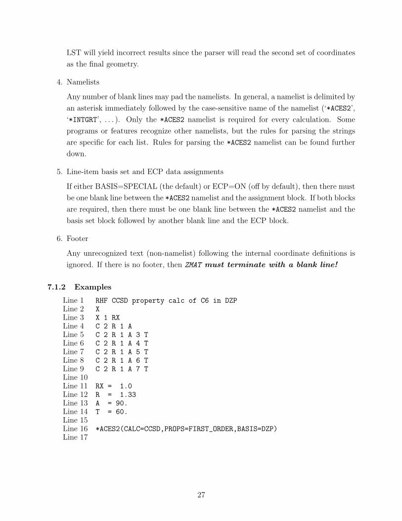
7.1.2 Examples
Line 1 RHF CCSD property calc of C6 in DZPLine 2 XLine 3 X 1 RXLine 4 C 2 R 1 ALine 5 C 2 R 1 A 3 TLine 6 C 2 R 1 A 4 TLine 7 C 2 R 1 A 5 TLine 8 C 2 R 1 A 6 TLine 9 C 2 R 1 A 7 TLine 10Line 11 RX = 1.0Line 12 R = 1.33Line 13 A = 90.Line 14 T = 60.Line 15Line 16 *ACES2(CALC=CCSD,PROPS=FIRST_ORDER,BASIS=DZP)Line 17
27
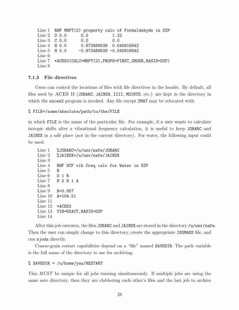
Line 1 RHF MBPT(2) property calc of Formaldehyde in DZPLine 2 O 0.0 0.0 1.22Line 3 C 0.0 0.0 0.0Line 4 H 0.0 0.873489539 0.545816842Line 5 H 0.0 -0.873489539 -0.545816842Line 6Line 7 *ACES2(CALC=MBPT(2),PROPS=FIRST_ORDER,BASIS=DZP)Line 8
7.1.3 File directives
Users can control the locations of files with file directives in the header. By default, all
files used by ACES II (JOBARC, JAINDX, IIII, MOINTS, etc.) are kept in the directory in
which the xaces2 program is invoked. Any file except ZMAT may be relocated with:
% FILE=/some/absolute/path/to/the/FILE
in which FILE is the name of the particular file. For example, if a user wants to calculate
isotopic shifts after a vibrational frequency calculation, it is useful to keep JOBARC and
JAINDX in a safe place (not in the current directory). For water, the following input could
be used:
Line 1 %JOBARC=/u/usr/safe/JOBARCLine 2 %JAINDX=/u/usr/safe/JAINDXLine 3Line 4 RHF SCF vib freq calc for Water in DZPLine 5 HLine 6 O 1 RLine 7 H 2 R 1 ALine 8Line 9 R=0.957Line 10 A=104.51Line 11Line 12 *ACES2Line 13 VIB=EXACT,BASIS=DZPLine 14
After this job executes, the files JOBARC and JAINDX are stored in the directory /u/usr/safe.
Then the user can simply change to this directory, create the appropriate ISOMASS file, and
run xjoda directly.
Coarse-grain restart capabilities depend on a “file” named SAVEDIR. The path variable
is the full name of the directory to use for archiving.
% SAVEDIR = /u/home/yau/RESTART
This MUST be unique for all jobs running simultaneously. If multiple jobs are using the
same save directory, then they are clobbering each other’s files and the last job to archive
28
its files is the one that wins. The default action is to create a directory named SAVEDIR in
the run directory.
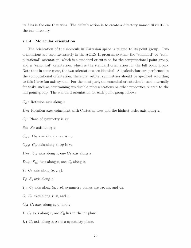
7.1.4 Molecular orientation
The orientation of the molecule in Cartesian space is related to its point group. Two
orientations are used extensively in the ACES II program system: the “standard” or “com-
putational” orientation, which is a standard orientation for the computational point group,
and a “canonical” orientation, which is the standard orientation for the full point group.
Note that in some cases, the two orientations are identical. All calculations are performed in
the computational orientation; therefore, orbital symmetries should be specified according
to this Cartesian axis system. For the most part, the canonical orientation is used internally
for tasks such as determining irreducible representations or other properties related to the
full point group. The standard orientation for each point group follows
CN : Rotation axis along z.
DN : Rotation axes coincident with Cartesian axes and the highest order axis along z.
Cs: Plane of symmetry is xy.
SN : SN axis along z.
CNv: CN axis along z, xz is σv.
CNh: CN axis along z, xy is σh.
DNh: CN axis along z, one C2 axis along x.
DNd: S2N axis along z, one C2 along x.
T : C3 axis along (q, q, q).
Td: S4 axis along z.
Th: C3 axis along (q, q, q), symmetry planes are xy, xz, and yz.
O: C4 axes along x, y, and z.
Oh: C4 axes along x, y, and z.
I: C5 axis along z, one C3 lies in the xz plane.
Ih: C5 axis along z, xz is a symmetry plane.
29
For groups with ambiguities (D2, D2h, C2v), there is no standard orientation at present,
and users might want to run xjoda once to show which orientation is used before assigning
orbital symmetries. For example, water belongs to the C2v point group and the symme-
try plane containing the hydrogen atoms might be assigned to either the xz or yz planes,
leading to an ambiguity between the b1 and b2 irreducible representations. Eventually, some
criterion could be established that can define a standard orientation for these groups thereby
alleviating this issue.
7.1.5 Dummy and ghost atoms
Dummy atoms, represented with “X”, are only useful for internal coordinates and define
points in space. They do not have basis functions and do not affect the symmetry of the
molecule. They are necessary to break angles of 180◦ and are used to define highly symmetric
molecules with no atom at the center of mass.
Ghost atoms, which are specified by the symbol “GH”, have zero nuclear charge. However,
while dummy atoms are “invisible” to the program outside the coordinate generator, ghost
atoms serve as a center for basis functions. This feature is particularly useful for calculations
that determine the basis set superposition error (BSSE) and has several other applications,
such as describing “lone-pair” electrons of a molecule by functions that are not centered at
any of the molecular nuclei. Symmetry can be used in such calculations but is restricted to
the symmetry of the “supermolecule” comprised of the real and ghost atoms. The additional
basis functions do not necessarily form a complete set of symmetry-adapted functions within
the point group of the supermolecule. This is different from the use of dummy atoms, which
do not affect the symmetry of the calculation.
Currently, only single point energy calculations are possible with ghost atoms. In ad-
dition, the basis set must be supplied explicitly with BASIS=SPECIAL and the line-item
basis set definitions after the *ACES2 namelist.
7.1.6 Cartesian coordinates
The format is straightforward. Each line defines one atom with the atomic symbol and
the values of the x, y, and z coordinates in free format. The coordinates may be given in
either atomic units or Angstroms.
Older versions of xjoda require COORDINATE=CARTESIAN for this to work, but any
version after 2.5.0 attempts to figure it out automatically (since the first line of a Z matrix
has only one word). If the Cartesian coordinates are specified in atomic units, then the
keyword UNITS=BOHR must be used.
30
7.1.7 Internal coordinates
The specification by internal coordinates is known as the Z matrix. Centers of the nuclei
are expressed relative to previously defined centers by means of distances and angles. The
specification includes a length, a bond angle, and a dihedral angle. The number associated
with each atom is governed by its position in the Z matrix. The essentials of Z matrix
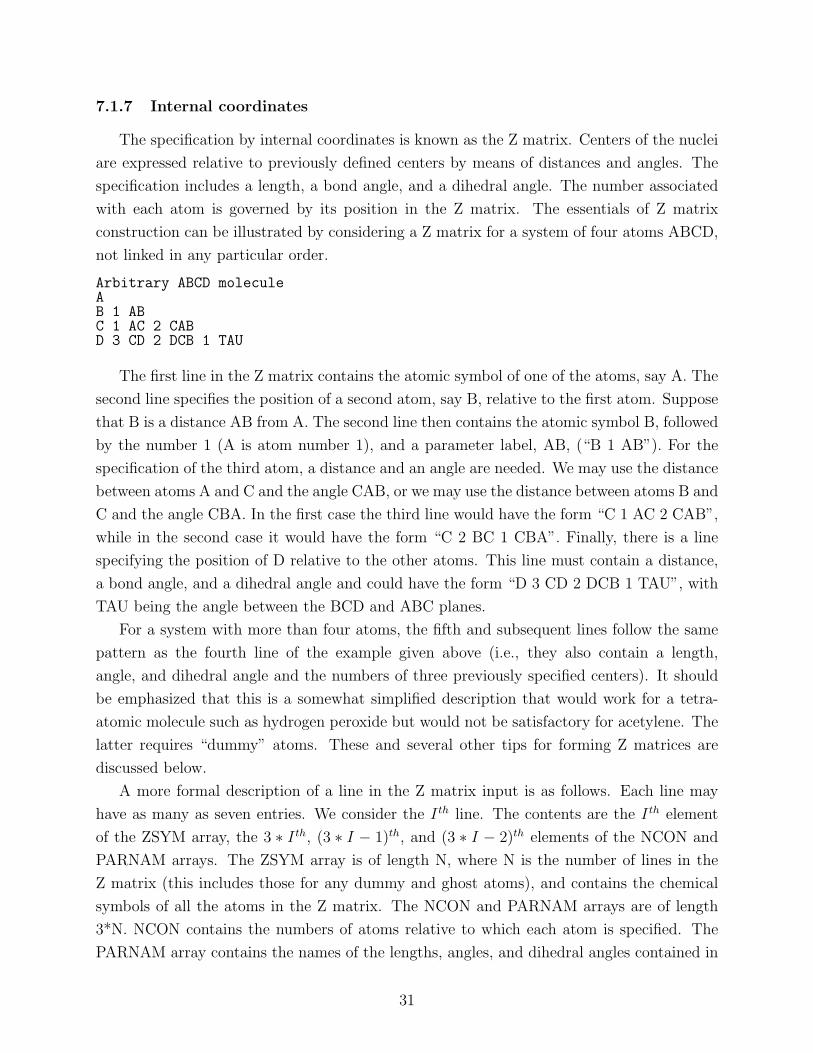
construction can be illustrated by considering a Z matrix for a system of four atoms ABCD,
not linked in any particular order.
Arbitrary ABCD moleculeAB 1 ABC 1 AC 2 CABD 3 CD 2 DCB 1 TAU
The first line in the Z matrix contains the atomic symbol of one of the atoms, say A. The
second line specifies the position of a second atom, say B, relative to the first atom. Suppose
that B is a distance AB from A. The second line then contains the atomic symbol B, followed
by the number 1 (A is atom number 1), and a parameter label, AB, (“B 1 AB”). For the
specification of the third atom, a distance and an angle are needed. We may use the distance
between atoms A and C and the angle CAB, or we may use the distance between atoms B and
C and the angle CBA. In the first case the third line would have the form “C 1 AC 2 CAB”,
while in the second case it would have the form “C 2 BC 1 CBA”. Finally, there is a line
specifying the position of D relative to the other atoms. This line must contain a distance,
a bond angle, and a dihedral angle and could have the form “D 3 CD 2 DCB 1 TAU”, with
TAU being the angle between the BCD and ABC planes.
For a system with more than four atoms, the fifth and subsequent lines follow the same
pattern as the fourth line of the example given above (i.e., they also contain a length,
angle, and dihedral angle and the numbers of three previously specified centers). It should
be emphasized that this is a somewhat simplified description that would work for a tetra-
atomic molecule such as hydrogen peroxide but would not be satisfactory for acetylene. The
latter requires “dummy” atoms. These and several other tips for forming Z matrices are
discussed below.
A more formal description of a line in the Z matrix input is as follows. Each line may
have as many as seven entries. We consider the I th line. The contents are the I th element
of the ZSYM array, the 3 ∗ I th, (3 ∗ I − 1)th, and (3 ∗ I − 2)th elements of the NCON and
PARNAM arrays. The ZSYM array is of length N, where N is the number of lines in the
Z matrix (this includes those for any dummy and ghost atoms), and contains the chemical
symbols of all the atoms in the Z matrix. The NCON and PARNAM arrays are of length
3*N. NCON contains the numbers of atoms relative to which each atom is specified. The
PARNAM array contains the names of the lengths, angles, and dihedral angles contained in
31
the Z matrix. Positions 3∗ I−2 are for lengths, 3∗ I−1 for angles, and 3∗ I are for dihedral
angles (I=1,2,...,N). It should be clear that elements 1, 2, 3, and 5, 6, and 9 of NCON and
PARNAM are not defined. The I th line (I=1,2,...,N) then has the general form:
ZSYM The atomic symbol of the atom (dummy atom is “X”, ghost is “GH”).
NCON(3*I-2) The number of the atomic center to which the atom is formally linked.
Note that this need only be a formal link, the two atoms need not be chemically bonded.
(Only for I>1).
PARNAM(3*I-2) A character variable name corresponding to the distance between atom
NCON(3*I-2) and atom I.
NCON(3*I-1) The third member of the triangle formed by atoms I and NCON(3*I-2).
(Only for I>2).
PARNAM(3*I-1) A character variable corresponding to the associated angle.
NCON(3*I) The fourth member of the dihedral angle formed by atoms I, NCON(3*I-2),
and NCON(3*I-1). (Only for I>3).
PARNAM(3*I) A character variable name corresponding to a dihedral angle determined
as follows: In the plane perpendicular to the NCON(3*I-2)↔NCON(3*I-1) axis, the
angle is that needed to rotate the projection of the [I←NCON(3*I-2)] vector into
the projection of the [NCON(3*I)←NCON(3*I-1)] vector. Clockwise is taken to be
positive. Values must be restricted from -180 to 180◦.
All variable names (PARNAM array) are limited to five characters. An asterisk (∗)immediately after the variable name implies an optimization. No numbers are allowed inside
the Z matrix—all internal coordinates must be given a symbol, even if the value is not going
to be optimized.
Z matrix Parameters
After a blank line following the Z matrix, the values of all unique internal coordinates
(those with different names) are specified as follows:
PNM=Value
where PNM is one of the unique members of the PARNAM array (see above), and Value
is the value assigned to that coordinate. The first non-blank string after the equal sign is
passed to a number parser, so trailing text (like a comment) is ignored.
Angles must be entered in degrees (◦), and bond angles (as distinct from dihedral angles)
of 0◦ and 180◦ are not allowed since these lead to a singularity in the transformation between
32
Cartesian and internal coordinates (and do not allow dihedral angles to be defined). This,
of course, does not mean that ACES II is unable to handle linear molecules such as carbon
dioxide. Rather, for linear molecules, “dummy atoms” must be used in the Z matrix to avoid
problematic bond angles.
To facilitate construction of Z matrices for highly symmetric molecules, certain variable
names have been reserved for specific values. To use these parameters, which are listed
below, the user must specify a value in the parameter input section, but it need not be
correct since it will be converted to the exact value internally.
TDA Specifies the tetrahedral angle, Cos−1(−13
)(i.e., 109.4712. . . ).
IHA Specifies the “icosahedral” angle Cos−1(√
15
)(i.e., 63.4349. . .).
7.1.8 Z matrix analyzer
A unique feature of ACES II is the Z matrix analyzer, which is capable of detecting
subtle and obvious deficiencies in the definition of internal coordinates. This is particularly
important for geometry optimizations, in which the construction of the Z matrix and the
choice of parameters to be optimized are of vital importance. The analyzer inspects the
internal coordinates and carries out a number of checks. These include determination of
whether coordinates given the same name are actually equivalent or coordinates having
different names are equivalent, whether a non-zero gradient is possible with respect to modes
which are not being optimized, etc. In addition, it determines the number of degrees of
freedom within the totally symmetric subspaces of nuclear configurations and compares this
value with the number of independent coordinates which are being optimized. If they are
not equal, a warning message is printed out.
For most Z matrices with poorly defined internal coordinates, the analyzer prints out a
number of warning messages but does not halt the ACES II execution sequence. However,
for Z matrices which are particularly bad, it will terminate the job. All users are encouraged
to carefully inspect the output of the analyzer and to check that the full molecular point
group (printed out below the output from the analyzer) is the one intended. If warning
messages are printed or if the symmetry is not what the user expects, then reconstruct as
necessary.
A rule of thumb for Z matrix construction is that each internal coordinate included in
the Z matrix must be accompanied by all others which are equivalent to it by the symmetry
of the molecule. For example, in water, it is best to specify the molecular geometry by
the two O–H distances and the H–O–H bond angle, rather than by the O–H distance, the
H–H distance, and the H–H–O angle. Although most users would definitely use the first Z
matrix, the idea of using just chemical bonds as internuclear distances can be dangerous.
33
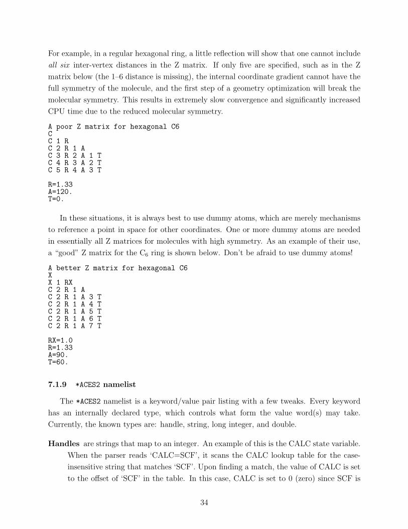
For example, in a regular hexagonal ring, a little reflection will show that one cannot include
all six inter-vertex distances in the Z matrix. If only five are specified, such as in the Z
matrix below (the 1–6 distance is missing), the internal coordinate gradient cannot have the
full symmetry of the molecule, and the first step of a geometry optimization will break the
molecular symmetry. This results in extremely slow convergence and significantly increased
CPU time due to the reduced molecular symmetry.
A poor Z matrix for hexagonal C6CC 1 RC 2 R 1 AC 3 R 2 A 1 TC 4 R 3 A 2 TC 5 R 4 A 3 T
R=1.33A=120.T=0.
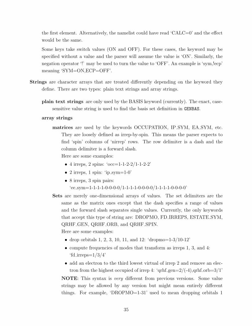
In these situations, it is always best to use dummy atoms, which are merely mechanisms
to reference a point in space for other coordinates. One or more dummy atoms are needed
in essentially all Z matrices for molecules with high symmetry. As an example of their use,
a “good” Z matrix for the C6 ring is shown below. Don’t be afraid to use dummy atoms!
A better Z matrix for hexagonal C6XX 1 RXC 2 R 1 AC 2 R 1 A 3 TC 2 R 1 A 4 TC 2 R 1 A 5 TC 2 R 1 A 6 TC 2 R 1 A 7 T
RX=1.0R=1.33A=90.T=60.
7.1.9 *ACES2 namelist
The *ACES2 namelist is a keyword/value pair listing with a few tweaks. Every keyword
has an internally declared type, which controls what form the value word(s) may take.
Currently, the known types are: handle, string, long integer, and double.
Handles are strings that map to an integer. An example of this is the CALC state variable.
When the parser reads ‘CALC=SCF’, it scans the CALC lookup table for the case-
insensitive string that matches ‘SCF’. Upon finding a match, the value of CALC is set
to the offset of ‘SCF’ in the table. In this case, CALC is set to 0 (zero) since SCF is
34
the first element. Alternatively, the namelist could have read ‘CALC=0’ and the effect
would be the same.
Some keys take switch values (ON and OFF). For these cases, the keyword may be
specified without a value and the parser will assume the value is ‘ON’. Similarly, the
negation operator ‘!’ may be used to turn the value to ‘OFF’. An example is ‘sym,!ecp’
meaning ‘SYM=ON,ECP=OFF’.
Strings are character arrays that are treated differently depending on the keyword they
define. There are two types: plain text strings and array strings.
plain text strings are only used by the BASIS keyword (currently). The exact, case-
sensitive value string is used to find the basis set definition in GENBAS.
array strings
matrices are used by the keywords OCCUPATION, IP SYM, EA SYM, etc.
They are loosely defined as irrep-by-spin. This means the parser expects to
find ‘spin’ columns of ‘nirrep’ rows. The row delimiter is a dash and the
column delimiter is a forward slash.
Here are some examples:
• 4 irreps, 2 spins: ‘occ=1-1-2-2/1-1-2-2’
• 2 irreps, 1 spin: ‘ip sym=1-0’
• 8 irreps, 3 spin pairs:
‘ee sym=1-1-1-1-0-0-0-0/1-1-1-1-0-0-0-0/1-1-1-1-0-0-0-0’
Sets are merely one-dimensional arrays of values. The set delimiters are the
same as the matrix ones except that the dash specifies a range of values
and the forward slash separates single values. Currently, the only keywords
that accept this type of string are: DROPMO, FD IRREPS, ESTATE SYM,
QRHF GEN, QRHF ORB, and QRHF SPIN.
Here are some examples:
• drop orbitals 1, 2, 3, 10, 11, and 12: ‘dropmo=1-3/10-12’
• compute frequencies of modes that transform as irreps 1, 3, and 4:
‘fd irreps=1/3/4’
• add an electron to the third lowest virtual of irrep 2 and remove an elec-
tron from the highest occupied of irrep 4: ‘qrhf gen=2/(-4),qrhf orb=3/1’
NOTE: This syntax is very different from previous versions. Some value
strings may be allowed by any version but might mean entirely different
things. For example, ‘DROPMO=1-31’ used to mean dropping orbitals 1
35
and 31 from the correlated calculation. If that string was parsed by the new
xjoda, vtran would attempt to remove every orbital from 1 to 31.
(long) Integers are parsed in a fairly straightforward manner. For example, ‘print=1’ and
‘charge=-1’.
There is one special state variable that recognizes units appended to the value and
that is MEMORY. Recognized units are (b)ytes and (w)ords with SI prefixes (k)ilo,
(m)ega, and (g)iga. The scaling factor is 1024, not 1000.
Doubles are not used currently even though we have this capability, there are no key-
words with values of this type. Examples would be: ‘double1=1.’, ‘double2=-2.d0’,
‘double3=3.5e-6’.
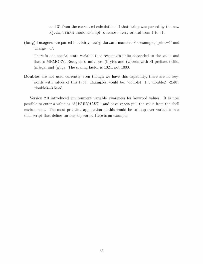
Version 2.3 introduced environment variable awareness for keyword values. It is now
possible to enter a value as “${VARNAME}” and have xjoda pull the value from the shell
environment. The most practical application of this would be to loop over variables in a
shell script that define various keywords. Here is an example:
36
> cat <<EOF >ZMATenvvar test jobHH 1 R
R=0.7
*ACES2calc=${CALC}basis=${BASIS}
EOF> for CALC in scf ccsd> do export CALC> for BASIS in DZP TZP TZ2P> do export BASIS> clean # or other cleaning script> xaces2 > $CALC.$BASIS.out> done> done> clean
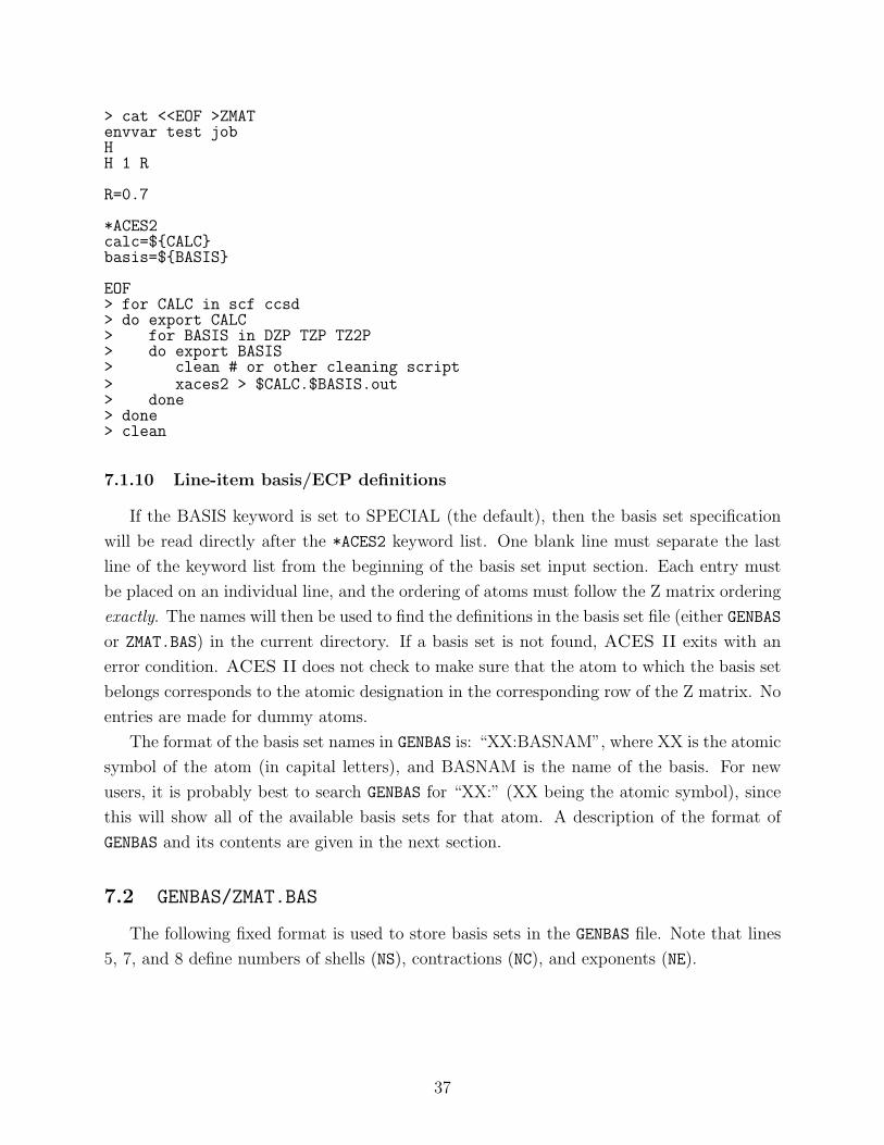
7.1.10 Line-item basis/ECP definitions
If the BASIS keyword is set to SPECIAL (the default), then the basis set specification
will be read directly after the *ACES2 keyword list. One blank line must separate the last
line of the keyword list from the beginning of the basis set input section. Each entry must
be placed on an individual line, and the ordering of atoms must follow the Z matrix ordering
exactly. The names will then be used to find the definitions in the basis set file (either GENBAS
or ZMAT.BAS) in the current directory. If a basis set is not found, ACES II exits with an
error condition. ACES II does not check to make sure that the atom to which the basis set
belongs corresponds to the atomic designation in the corresponding row of the Z matrix. No
entries are made for dummy atoms.
The format of the basis set names in GENBAS is: “XX:BASNAM”, where XX is the atomic
symbol of the atom (in capital letters), and BASNAM is the name of the basis. For new
users, it is probably best to search GENBAS for “XX:” (XX being the atomic symbol), since
this will show all of the available basis sets for that atom. A description of the format of
GENBAS and its contents are given in the next section.
7.2 GENBAS/ZMAT.BAS
The following fixed format is used to store basis sets in the GENBAS file. Note that lines
5, 7, and 8 define numbers of shells (NS), contractions (NC), and exponents (NE).
37
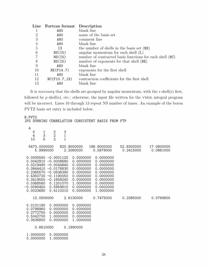
Line Fortran format Description1 A80 blank line2 A80 name of the basis set3 A80 comment line4 A80 blank line5 I3 the number of shells in the basis set (NS)6 NS(I5) angular momentum for each shell (L)7 NS(I5) number of contracted basis functions for each shell (NC)8 NS(I5) number of exponents for that shell (NE)9 A80 blank line10 NE(F14.7) exponents for the first shell11 A80 blank line12 NC(F10.7,1X) contraction coefficients for the first shell13 A80 blank line
It is necessary that the shells are grouped by angular momentum, with the s shell(s) first,
followed by p shell(s), etc.; otherwise, the input file written for the vmol integral program
will be incorrect. Lines 10 through 13 repeat NS number of times. An example of the boron
PVTZ basis set entry is included below.
B:PVTZJFS DUNNING CORRELATION CONSISTENT BASIS FROM FTP
40 1 2 34 3 2 1
10 5 2 1
5473.0000000 820.9000000 186.8000000 52.8300000 17.08000005.9990000 2.2080000 0.5879000 0.2415000 0.0861000
0.0005550 -0.0001120 0.0000000 0.00000000.0042910 -0.0008680 0.0000000 0.00000000.0219490 -0.0044840 0.0000000 0.00000000.0844410 -0.0176830 0.0000000 0.00000000.2385570 -0.0536390 0.0000000 0.00000000.4350720 -0.1190050 0.0000000 0.00000000.3419550 -0.1658240 0.0000000 0.00000000.0368560 0.1201070 1.0000000 0.0000000
-0.0095450 0.5959810 0.0000000 0.00000000.0023680 0.4110210 0.0000000 1.0000000
12.0500000 2.6130000 0.7475000 0.2385000 0.0769800
0.0131180 0.0000000 0.00000000.0798960 0.0000000 0.00000000.2772750 0.0000000 0.00000000.5042700 1.0000000 0.00000000.3536800 0.0000000 1.0000000
0.6610000 0.1990000
1.0000000 0.00000000.0000000 1.0000000
38
0.4900000
1.0000000
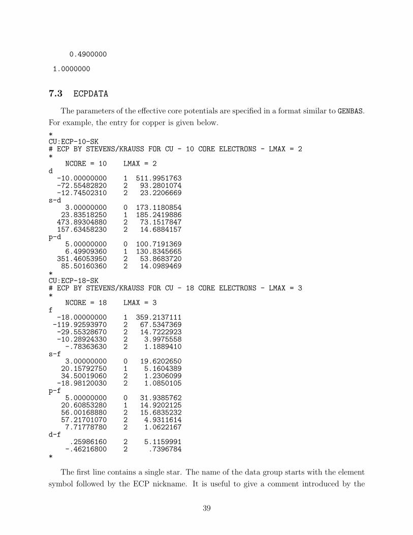
7.3 ECPDATA
The parameters of the effective core potentials are specified in a format similar to GENBAS.
For example, the entry for copper is given below.
*CU:ECP-10-SK# ECP BY STEVENS/KRAUSS FOR CU - 10 CORE ELECTRONS - LMAX = 2*
NCORE = 10 LMAX = 2d
-10.00000000 1 511.9951763-72.55482820 2 93.2801074-12.74502310 2 23.2206669
s-d3.00000000 0 173.1180854
23.83518250 1 185.2419886473.89304880 2 73.1517847157.63458230 2 14.6884157
p-d5.00000000 0 100.71913696.49909360 1 130.8345665
351.46053950 2 53.868372085.50160360 2 14.0989469
*CU:ECP-18-SK# ECP BY STEVENS/KRAUSS FOR CU - 18 CORE ELECTRONS - LMAX = 3*
NCORE = 18 LMAX = 3f
-18.00000000 1 359.2137111-119.92593970 2 67.5347369-29.55328670 2 14.7222923-10.28924330 2 3.9975558
-.78363630 2 1.1889410s-f
3.00000000 0 19.620265020.15792750 1 5.160438934.50019060 2 1.2306099
-18.98120030 2 1.0850105p-f
5.00000000 0 31.938576220.60853280 1 14.920212556.00168880 2 15.683523257.21701070 2 4.93116147.71778780 2 1.0622167
d-f.25986160 2 5.1159991
-.46216800 2 .7396784*
The first line contains a single star. The name of the data group starts with the element
symbol followed by the ECP nickname. It is useful to give a comment introduced by the
39
hash symbol (#) in the next line to indicate the origin of the ECP. The actual ECP data
is given in between two lines with a ‘∗’. The first line specifies the number of core electrons
described by the ECP (NCORE) and the maximum angular momentum number of the
projector operators (LMAX) in integers (s=0, p=1, d=2, . . . ). These are followed by the
description of the effective core potential which consists of the angular momentum numbers
and by the analytical representation of the operator. The latter includes the coefficient cm,
the exponent Nm of r and the exponent αm of the gaussian:
Ul(r) =∑m
cmeαmr2
rNm .
For a detailed description, see L.R. Kahn, P. Baybutt, and D.G. Truhlar, J. Chem. Phys.
65, 3826 (1976).
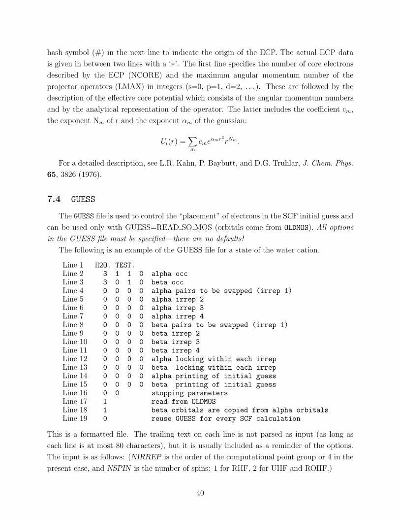
7.4 GUESS
The GUESS file is used to control the “placement” of electrons in the SCF initial guess and
can be used only with GUESS=READ SO MOS (orbitals come from OLDMOS). All options
in the GUESS file must be specified—there are no defaults!
The following is an example of the GUESS file for a state of the water cation.
Line 1 H2O. TEST.Line 2 3 1 1 0 alpha occLine 3 3 0 1 0 beta occLine 4 0 0 0 0 alpha pairs to be swapped (irrep 1)Line 5 0 0 0 0 alpha irrep 2Line 6 0 0 0 0 alpha irrep 3Line 7 0 0 0 0 alpha irrep 4Line 8 0 0 0 0 beta pairs to be swapped (irrep 1)Line 9 0 0 0 0 beta irrep 2Line 10 0 0 0 0 beta irrep 3Line 11 0 0 0 0 beta irrep 4Line 12 0 0 0 0 alpha locking within each irrepLine 13 0 0 0 0 beta locking within each irrepLine 14 0 0 0 0 alpha printing of initial guessLine 15 0 0 0 0 beta printing of initial guessLine 16 0 0 stopping parametersLine 17 1 read from OLDMOSLine 18 1 beta orbitals are copied from alpha orbitalsLine 19 0 reuse GUESS for every SCF calculation
This is a formatted file. The trailing text on each line is not parsed as input (as long as
each line is at most 80 characters), but it is usually included as a reminder of the options.
The input is as follows: (NIRREP is the order of the computational point group or 4 in the
present case, and NSPIN is the number of spins: 1 for RHF, 2 for UHF and ROHF.)
40
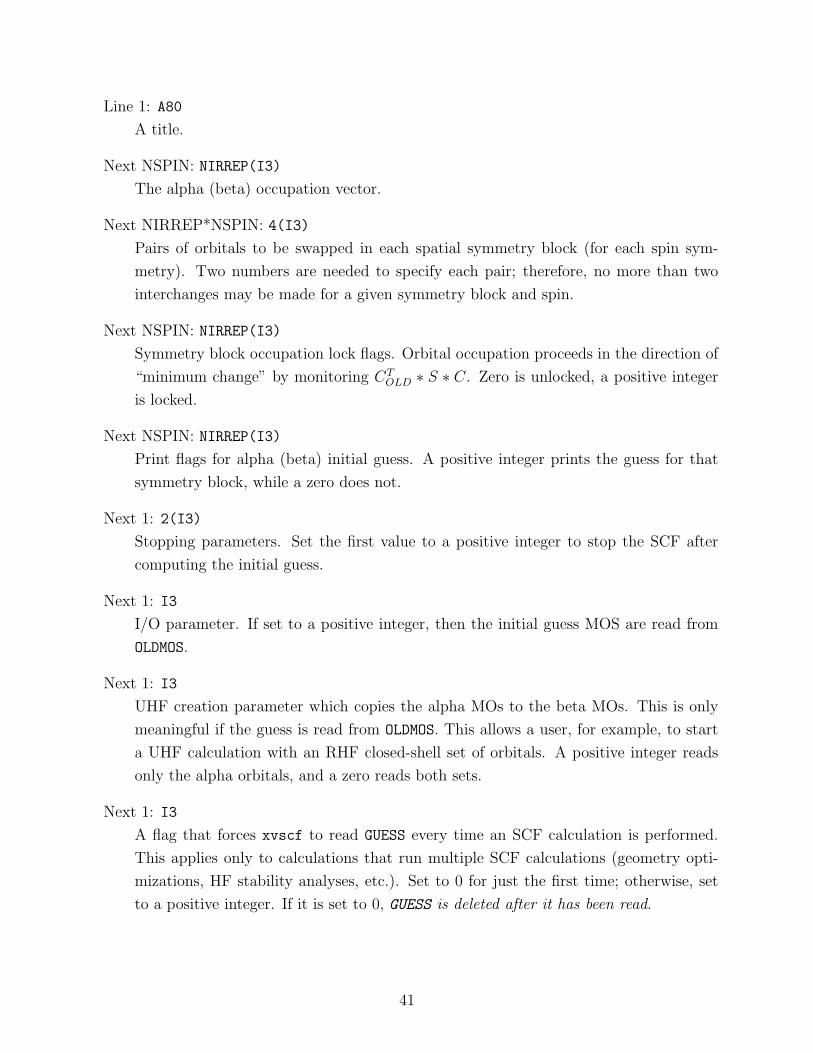
Line 1: A80
A title.
Next NSPIN: NIRREP(I3)
The alpha (beta) occupation vector.
Next NIRREP*NSPIN: 4(I3)
Pairs of orbitals to be swapped in each spatial symmetry block (for each spin sym-
metry). Two numbers are needed to specify each pair; therefore, no more than two
interchanges may be made for a given symmetry block and spin.
Next NSPIN: NIRREP(I3)
Symmetry block occupation lock flags. Orbital occupation proceeds in the direction of
“minimum change” by monitoring CTOLD ∗ S ∗ C. Zero is unlocked, a positive integer
is locked.
Next NSPIN: NIRREP(I3)
Print flags for alpha (beta) initial guess. A positive integer prints the guess for that
symmetry block, while a zero does not.
Next 1: 2(I3)
Stopping parameters. Set the first value to a positive integer to stop the SCF after
computing the initial guess.
Next 1: I3
I/O parameter. If set to a positive integer, then the initial guess MOS are read from
OLDMOS.
Next 1: I3
UHF creation parameter which copies the alpha MOs to the beta MOs. This is only
meaningful if the guess is read from OLDMOS. This allows a user, for example, to start
a UHF calculation with an RHF closed-shell set of orbitals. A positive integer reads
only the alpha orbitals, and a zero reads both sets.
Next 1: I3
A flag that forces xvscf to read GUESS every time an SCF calculation is performed.
This applies only to calculations that run multiple SCF calculations (geometry opti-
mizations, HF stability analyses, etc.). Set to 0 for just the first time; otherwise, set
to a positive integer. If it is set to 0, GUESS is deleted after it has been read.
41
8 Keywords
8.1 *ACES2 namelist
The user can control the behavior of an ACES II job through the use of keywords in the
*ACES2 namelist. In some cases, the value for a keyword can be specified by an integer or
by a character string. In our opinion the latter is preferable as it makes the input file more
readable.
All possible keywords in the *ACES2 namelist are discussed below. As there are a lot of
keywords, we have grouped them according to the general flow of a calculation.
Keyword Conventions
Keywords in the *ACES2 namelist are matched to an initial substring of the actual keyword
in xjoda. For example, the full keyword is CALCLEVEL, but the unique substring is CALC,
so CALC, CALCULATION, and CALCLEVEL may all be used to set the calculation level.
The underlined substring in the following keyword definitions is what is used to match the
keyword. As another example, the memory keyword is defined as MEMORY SIZE, but any
keyword in the *ACES2 namelist starting with MEM will be used to set the memory size.
Some keywords should not be set by the user without careful consideration of what the
program will do. Either the keyword controls experimental pathways through the program,
or the program uses considerable logic to determine the correct default behavior. These
keywords are listed in italics instead of bold.
Value Conventions
Value strings are parsed differently depending on how the corresponding keyword is de-
fined in joda. Currently, there are handles, strings, integers, and reals. For clarity, this
manual also mentions switches and tols (tolerances). A switch is a handle with only two
values (ON/OFF), and a tol is an integer N that corresponds to a value of 10−N .
In ACES II, handles are character strings that map onto integers. For example, the
CALC keyword has 41 possible values. The code might do one thing if CALC=0 (SCF)
and another if CALC=10 (CCSD). Keywords of type handle can accept the handle string or
the integer as a value, so CALC=CCSD does the same thing as CALC=10 in the namelist.
Ultimately, the internal integer is irrelevant to the user and could change any time; therefore,
all keywords are described according to their handles only.
Some keywords only recognize switch-like handles (TRUE/FALSE, ON/OFF, 1/0, etc.)
and are listed as type switch. If these keywords appear in the namelist without a value
string, then they will be set to ON. Similarly, they can be negated by prefixing them with an
exclamation mark. For example *ACES2(RESTART,!NONHF) will register as RESTART=ON
42
and NONHF=OFF.
Keywords of type string are self-explanatory; however, they are used to read in fixed-
format arrays until we define a general expression for array notation. Hopefully the formats
of keywords that accept arrays are clearly described in the manual.
Integers are also self-explanatory and can be used in place of handles for those keywords
of such type. As mentioned before, a tol type is an integer that corresponds to the negative
power of 10. Some keywords are defined with unusual units, and these are appropriately
identified in the manual.
Currently, reals apply only to memory-related keywords. These are identified as type
“special” because the parser will scale the real by units suffixed to the value string.
8.1.1 System: general
CALCLEVEL = (handle) SCF
Specifies the general level of theory to be used throughout the program. Acceptable
values are: SCF, MBPT(2), MBPT(3), SDQ-MBPT(4), MBPT(4), LCCD, LCCSD,
UCCSD(4), CCD, UCC(4), CCSD, CCSD[T], CCSD+TQ*, CCSDT-1, CCSDT-1b,
CCSDT-2, CCSDT-3, CCSDT-4, CCSDT, LCCSDT, CCD+ST(CCD), QCISD(T),
CCSD(T), QCISD, CID, CISD, QCISD(TQ), CCSD(TQ), CCSD+TQ, CCSDT+Q*,
CCSDT+Q, CC5SD(T), CCSD-T, CC3, CCSDT-T1T2, CCSDTQ-1, CCSDTQF-1,
CCSDTQ-2, CCSDTQ-3, CCSDTQ, ACCSD, and HFDFT. Emphasized calculation
levels (in italics) are not implemented currently but are planned for future versions of
the program. CALC=HFDFT has been obsoleted by SCF TYPE=KS.
MEMORY SIZE = (special) 15000000W
Sets the “maximum” memory to allocate. Most member executables will not allocate
more than the amount specified, but some will attempt to allocate extra bits (on the
order of a few megabytes) that are of little consequence compared to the main memory
heap.
There is special parsing logic for the corresponding value string. The tail of the string is
checked for case-insensitive units and optional prefixes. Units can be W (integer words)
or B (bytes), and prefixes can be K, M, or G (kilo, mega, and giga, respectively). The
number part is read with the atof() C function.
[NOTE: The prefixes scale the units by 210 (1024), not 1000, and the default unit is
integer words (4 bytes for 32-bit binaries and 8 bytes for 64-bit binaries).]
RESTART = (switch) ON
43
Controls the creation, updating, and reading of a checkpoint directory. Currently,
only coarse-grain restarts are available, which means geometry optimizations and finite
difference calculations can be restarted from the last checkpoint. Fine-grain restarts
are not available yet but will also checkpoint SCF, T, and Lambda iterations.
GRAD CALC = (handle) AUTO
Specifies whether to calculate a gradient analytically or numerically. This should be
used only to override analytical gradients since the program will attempt to use them
whenever possible.
DERIV LEV = (handle) -1
Specifies whether or not derivatives of the energy are to be calculated and if so then
whether first or second. =NONE Derivatives not calculated, =FIRST First derivatives
to be calculated, =SECOND Second derivatives to be calculated. This is automatically
set.
8.1.2 System: molecular control
SYMMETRY = (handle) ON
Specifies which subgroup (“computational” point group) of the full point group is to
be used in the energy and/or gradient calculation. =OFF forces a no symmetry run
(in C1), =ON runs the calculation in the largest self-adjoint subgroup (D2h and its
subgroups), and =FULL uses the full point group. Currently, ACES II does not
support groups with degenerate representations, so the FULL option has no value
unless joda is used to make input files for another program package.
SUBGROUP = (handle) DEFAULT
Specifies a lower computational point group symmetry to use (provided it is a subgroup
of the full group). Acceptable values are: DEFAULT, C1, C2, CS, CI, C2V, C2H,
D2, and D2H. SUBGROUP=C1 is equivalent to SYMMETRY=OFF. The DEFAULT
option uses the highest order Abelian subgroup (including the full group).
SUBGRPAXIS = (handle) X
This is a somewhat complicated keyword to use. The value can be X, Y, or Z. The
use of the keyword is best described by example: Suppose one is running a calculation
on water, and wishes to run it in the Cs point group with the “special” plane being
the one that bisects the H-O-H bond angle. SUBGRPAXIS specifies which Cartesian
direction in the C2v frame becomes the special direction in the Cs frame. Normally,
44
joda will orient water in the yz plane. In this example, the y axis in the C2v frame
should be the z axis in the Cs frame, so SUBGRPAXIS=Z.
When the true Abelian subgroup is either C2v or D2h, the orientation is not well
defined, and it might be necessary to run xjoda twice. If SUBGROUP=0 in the first
pass, then the reference orientation for the true Abelian subgroup can be determined
and the appropriate value of SUBGRPAXIS can be selected.
NOREORI = (switch) OFF
Forces the program not to change the internal orientation of the molecule specified
by the input Cartesian coordinates. To function correctly, this keyword also requires
turning off symmetry (SYMMETRY=OFF).
8.1.3 System: debug
PRINT = (integer) 0
Controls the amount of printing in all member executables except joda. A value of
1 will produce a modest amount of additional output over the default value, which
includes some useful information such as SCF eigenvectors.
JODA PRINT = (integer) 0
Controls the amount of debug printing performed by joda. The higher the value, the
more information is printed. Values of 25 or higher generally do not produce anything
of interest to the general user, and values greater than 999 will dump the core vector
to disk.
8.1.4 I/O subsystem
FILE RECSIZ = (special) -1W
Sets the length of the physical records used in direct access file I/O. This value should
always be chosen as a multiple of 512 bytes and is parsed like the MEMORY SIZE key-
word. The default value (-1) determines a size based on the value of MEMORY SIZE.
CACHE RECS = (integer) -1
Sets the number of physical records (of length FILE RECSIZE) held in the I/O cache.
The maximum number of records is 128, and the default value (-1) determines a number
based on the value of MEMORY SIZE.
INCORE = (handle) NONE
45
This keyword can be used to reduce disk I/O (usually by a significant amount). Ac-
ceptable values are: NONE, NOABCD, NOABCI, NOABIJ, ALL, and T. =NONE and
=ALL load no and all lists into core memory, respectively. =NOABCD, =NOABCI,
and =NOABIJ load all lists that are at most the size of 〈Ab|Ci〉, 〈Ab|Ij〉, and 〈Ij|Ka〉molecular integral lists, respectively. These options are implemented in vcc, lambda,
dens, anti, bcktrn, and vee. The =T option only applies to vcc, which will load T1
and T2 amplitudes into memory. All of the other executables will treat =T as =NONE
(including lambda, although this should change soon).
8.1.5 Chemical system
COORDINATES = (handle) AUTO
Specifies whether the molecular system is defined in INTERNAL (Z matrix) or CARTE-
SIAN (xyz) coordinates.
UNITS = (handle) ANGSTROM
Specifies the units used for molecular geometries. The value can be ANGSTROM or
BOHR.
CHARGE = (integer) 0
Sets the molecular charge.
MULTIPLICTY = (integer) 1
Sets the spin multiplicity (2S + 1).
8.1.6 Basis set
BASIS = (string) SPECIAL
Defines the name of the basis set to use for all atoms in the molecule. If BA-
SIS=SPECIAL, then each atom (in coordinate order) must be specified after the
*ACES2 namelist.
SPHERICAL = (switch) OFF
Controls whether (=ON) spherical harmonic (5d, 7f, 9g, ...) or (=OFF) Cartesian (6d,
10f, 15g, ...) basis functions are used.
LINDEP TOL = (tol) 5
Sets the tolerance for linear dependencies in the basis set. The basis set is considered
linearly dependent and eigenvectors of the overlap matrix are neglected if the associated
eigenvalues are less than 10−N .
46
GENBAS 1 = (integer) 0
This keyword applies to first-row elements (H and HE) and specifies the number of
contracted Gaussian functions per shell. There is usually no need to use this keyword,
but it can be useful for using a subset of the functions in a particular entry in the
GENBAS file, particularly for generally contracted basis sets. For example, if entry
H:BASIS in the GENBAS file contains 7 contracted s functions, 4 p functions, and one
d function, then setting GENBAS 1=730 would eliminate the last p function and the
d function. The default for this keyword is to use the unaltered entry in GENBAS.
GENBAS 2 = (integer) 0
This keyword performs the same function as GENBAS 1 but applies only to second-row
atoms.
GENBAS 3 = (integer) 0
This keyword performs the same function as GENBAS 1 and GENBAS 2, but applies
only to third-row atoms.
CONTRACTION = (handle) GENERAL
Specifies the contraction scheme used by the integral and integral derivative programs.
This can be set to SEGMENTED or GENERAL.
[NOTE: Even for truly segmented basis sets, both integral and integral derivative
programs run significantly faster in GENERAL mode.]
ECP = (switch) OFF
Controls whether effective core potentials (a kind of pseudopotential) are used (=ON)
or not (=OFF). ECP=ON requires BASIS=SPECIAL and specification of the ECP
data sets (in a file named ECPDATA).
8.1.7 Integrals
INTEGRALS = (handle) VMOL
Specifies which integral package to use. This is not a very robust keyword and should
always be set to VMOL unless otherwise directed to change it. Other values include
SEWARD and GAMESS, but these options will not work unless the binaries were
linked to the appropriate libraries, which require third-party license agreements.
INTGRL TOL = (tol) 14
Sets the tolerance for storing the two-electron integrals such that integrals having an
absolute value greater than 10−N will be stored on disk.
47
DIRECT = (switch) OFF
Controls whether two-particle AO integrals are calculated on-the-fly or calculated once
and stored in a file. This cannot be used with VMOL integrals.
8.1.8 Reference
REFERENCE = (handle) RHF
Specifies the type of SCF reference to use. Supported references include spin-restricted
Hartree-Fock (=RHF), spin-unrestricted Hartree-Fock (=UHF), and spin-restricted
open-shell Hartree-Fock (=ROHF). These apply to Kohn-Sham DFT references as well
(e.g., RHF is spin-restricted Kohn-Sham). REF=TWODET (two-determinant refer-
ence for open-shell singlet CC calculations) is available, but the orbitals are obtained
from a closed-shell state and are not optimum open-shell singlet (or low spin triplet)
SCF orbitals. The orbital occupancy for subsequent CCSD calculations is specified by
the various QRHF keywords.
NONHF = (switch) OFF
Signals the correlation energy code if the reference wavefunction satisfies the Hartree-
Fock equations (Fai = 0). Usually there is no need to set this keyword since standard
non-HF reference functions (QRHF and ROHF) set this flag internally; however, if
you input a set of orbitals to the correlation energy code directly, then it might be
necessary to set NONHF=ON.
ORBITALS = (handle) -1
Specifies semicanonical orbitals (Fi6=j = Fa 6=b = 0) in non-HF calculations. “Semi-
canonical” orbitals are obtained by diagonalizing the occupied-occupied (ij) and virtual-
virtual (ab) blocks of the spin-orbital Fock matrix and can be advantageously exploited
in certain post-SCF calculations. (This is particularly true for ROHF-MBPT and non-
iterative triple excitation corrections.) There is no default value for this parameter,
and considerable logic is used to determine the orbital type in post-SCF non-HF cal-
culations (if the keyword is not defined). It is strongly recommended that this key-
word not be used by anyone who is not thoroughly familiar with non-HF CC/MBPT
methods, since the logic used to set the default value is sound. =STANDARD uses
the orbitals obtained in the reference function calculation without modification, and
=SEMICANONICAL forces a transformation to semicanonical orbitals.
PERT ORB = (handle) UNKNOWN
48
Specifies whether the gradient formulation assumes that the perturbed orbitals are not
those in which the Fock matrix is diagonal (=STANDARD). =CANONICAL means
that the perturbed orbitals are assumed to be canonical. This keyword must be set
to CANONICAL in gradient calculations with methods that include triple excitations
(i.e., MBPT(4), CCSD[T], CCSD(T), and QCISD(T)).
8.1.9 SCF: general
SCF TYPE = (handle) HF
Switches the SCF code between the standard Hartree-Fock program (=HF) and the
Kohn-Sham DFT program (=KS). If SCF TYPE=KS, then the KS-DFT program gen-
erates the SCF reference and requires separate namelists (viz. *VSCF and *INTGRT).
FOCK = (handle) PK
Specifies the algorithm for constructing the Fock matrix in SCF calculations. =PK
uses the PK-supermatrix approach while =AO constructs the matrix directly from the
AO integrals. In general, PK is faster but results in considerable use of disk space
when out-of-core algorithms are required.
CHECK SYM = (handle) OVERRIDE
Specifies the action taken when the density matrix does not transform as the totally
symmetric irreducible representation of the full molecular point group. =NORMAL
terminates the run if the molecule is nonlinear, while =OVERRIDE allows the job to
continue but prints a warning message. Nonsymmetric density matrices result from
calculations on electronically degenerate states or from broken-symmetry SCF solu-
tions. Often, such calculations do not give meaningful results and inexperienced users
are encouraged to use CHECK SYM=NORMAL in their calculations on nonlinear
molecules. For Π, ∆, Φ, ... states of linear molecules, however, meaningful calculations
can still be performed even though the density matrix is not symmetric.
SCF PRINT = (integer) 0
[This keyword is currently not used but exists for future compatibility.]
8.1.10 SCF: orbital control
GUESS = (handle) MOREAD
Specifies where the initial SCF eigenvectors are read from. The HF-SCF executable
checks multiple places for pre-existing orbitals, but this keyword can override that
logic.
49
=MOREAD → JOBARC file
=CORE → core Hamiltonian
=READ SO MOS → OLDMOS file (from NEWMOS)
=READ AO MOS → OLDAOMOS file (from AOBASMOS)
Other options include =NDDO, =WALT PRJDEN, =MIN BASIS, and =HUCKEL,
although some of these are still experimental and not fully supported.
OCCUPATION = (string of irrep-by-spin array)
Specifies the orbital occupancy of the reference wavefunction in terms of the occupation
numbers per irrep per spin. The occupancy is specified by NIRREP (or 2*NIRREP)
integers that define the number of occupied orbitals of each symmetry type. (NIRREP
is the number of irreducible representations in the computational point group.) If
there are no orbitals of a particular symmetry type, then a zero must be entered. If
the reference wavefunction is for an open-shell system, then two strings of NIRREP
occupation numbers separated by a forward-slash (/) define the α and β sets of orbitals.
An example of the use of the OCCUPATION keyword for the water molecule would be
OCCUPATION=3-1-1-0. For the 2A1 water cation (an open-shell system), the keyword
would be specified by OCCUPATION=3-1-1-0/2-1-1-0.
It should be noted that the VMOL integral program orders the irreducible representa-
tions in a strange way, which most users do not perceive to be a logical order. Hence,
it is advised to run a single-point SCF calculation to determine the initial number
and ordering of the irreducible representations. The occupation keyword may be omit-
ted, in which case an initial orbital occupancy is determined by diagonalizing the core
Hamiltonian. In many cases, SCF calculations that use the core Hamiltonian guess
will converge to the lowest energy SCF solution, but this is not guaranteed.
LOCK ORBOCC = (switch) OFF
Controls orbital occupancies among symmetry blocks in the SCF iterations. =ON locks
the occupation to the OCCUPATION value array (or the initial guess if OCCUPATION
is undefined); =OFF permits the occupation to change.
[NOTE: If the OCCUPATION keyword is defined, then LOCK ORBOCC is switched
on automatically.]
NEWVRT = (switch) OFF
50
Signals if the SCF virtual orbitals are to be replaced by a set determined from an N−1
potential. This is an orthogonal transformation within the virtual space. As long as
appropriate fij and fab are included, the energies of standard single-reference methods
are unchanged. However, for TD-CC methods, this keyword mixes one of the occupied
orbitals with the virtual space and the results are changed. It is anticipated that TD-
CCSD calculations will be improved by the use of this keyword, but this has yet to
be demonstrated. NEWVRT is useful for interpreting results of EOM-EE calculations
since excitations tend to be more easily identified as involving one occupied and one
virtual orbital. =OFF does not rotate the virtual space, and =ON rotates the virtual
space.
8.1.11 SCF: iteration control
SCF CONV = (tol) 7
Sets the convergence criterion for the SCF equations. Equations are considered con-
verged when the maximum change in density matrix elements is less than 10−N .
SCF MAXCYC = (integer) 150
Sets the maximum number of SCF iterations.
DAMP TYP = (handle) NONE
Specifies what type of damping is used during the SCF iterations. The value can be
NONE (no damping), DAVIDSON (Davidson’s empirical dynamical damping scheme),
and STATIC (a fixed damping parameter). Note that RPP convergence extrapolation
is not turned on until the damp factor has gone below DAMP TOL and the energy
change is below 0.05 a.u. DAMP TYP=DAVIDSON is recommended even though
NONE is the default.
DAMP TOL = (integer) 10
If DAMP TYP=DAVIDSON, then the cutoff is defined to be N ∗ 0.01, so the default
cutoff is 0.1.
DAMPSCF = (integer) 20
If DAMP TYP=STATIC, then the static damping factor used in the SCF iterations is
N ∗ 0.01, so the default damping factor is 0.2.
SCF EXTRAP (previously RPP) = (switch) ON
Controls whether or not the reduced partitioning procedure is to be used to accelerate
convergence of the SCF equations.
51
SCF EXPORDER (previously RPP ORDER) = (integer) 6
Sets the number of density matrices to be used in the RPP convergence acceleration
procedure.
SCF EXPSTAR (previously RPP LATEST) = (integer) 8
Sets the latest iteration for initiation of the RPP convergence acceleration procedure.
RPP is switched on when the error falls below a certain threshold, but in difficult cases,
in which the iterations are oscillatory, it is necessary to force it on when the error is
still large. In these cases, the RPP will begin on the iteration number specified by this
parameter.
LSHF A1 = (integer) 0
Sets the doubles-singles level shifting parameter α, in which α = N∗0.01. This keyword
is currently only meaningful in ROHF calculations.
LSHF B1 = (integer) 0
Sets the singles-virtuals level shifting parameter β, in which β = N∗0.01. This keyword
is currently only meaningful in ROHF calculations.
8.1.12 SCF reference adjustments
DROPMO = (string of 1D array) 0
Lists which molecular orbitals will be dropped from the post-SCF calculation. The
orbitals are ordered by eigenvalue from the most stable (negative energy) to the most
unstable (largest positive energy) regardless of irrep. The delimiter is a forward-slash
(/) that separates single orbitals and orbital ranges (x-y inclusive). For example, the
string “1-5/55/62-64” will cause vtran to drop orbitals 1, 2, 3, 4, 5, 55, 62, 63, and
64. For UHF calculations, the appropriate orbitals are deleted from both spin cases.
HFSTABILITY = (handle) OFF
Checks the stability of RHF and UHF wavefunctions and optionally rotates the orbitals
to a lower SCF solution. There are three possible options for this keyword. =OFF
does nothing and =ON performs a stability check and returns the number of negative
eigenvalues in the orbital rotation Hessian. =FOLLOW performs the stability check
and then proceeds to rotate the SCF orbitals in the direction of a particular negative
eigenvalue of the orbital rotation Hessian (see the explanation of the ROT EVEC
keyword below), after which the SCF is rerun.
52
ROT EVEC = (integer) 0
Defines which eigenvector of the orbital rotation Hessian will be used to rotate the
original SCF orbitals. By default, it will use the eigenvector with the lowest eigenvalue
of irrep 1 (the totally symmetric part of the block-factored Hessian). This choice
often leads to the lowest energy SCF solution. For RHF stability checks, only those
instabilities which correspond to RHF solutions will be considered. It is important
to understand that following non-symmetric eigenvectors lowers the symmetry of the
wavefunction and that following RHF→UHF stabilities leads to a UHF solution. To
converge the SCF roots associated with such instabilities, one must run the calculation
in reduced symmetry and as a closed-shell UHF case, respectively. If not set to 0, the
program follows the vector with the N th lowest eigenvalue having the proper symmetry
(totally symmetric) and spin (RHF→RHF or UHF→UHF) properties.
BRUECKNER = (switch) OFF
Controls whether Brueckner orbitals are to be determined for the specified CC method.
BRUCK CONV = (tol) 4
Sets the convergence criterion in Brueckner iterations. The calculation is considered
converged when the largest single excitation amplitude falls below 10−N .
QRHF GENERAL = (string of 1D array) 0
The presence of this keyword turns on QRHF logic, and the value of each element
specifies which irrep is created (positive) or annihilated (negative). In the QRHF
scheme, an RHF (closed-shell) SCF calculation is performed with the OCCUPATION
keyword or the CHARGE and MULTIPLICITY keywords. The correlated calculation
is then performed on an open-shell reference generated from this closed-shell state
by removing, adding, or exciting electrons. Any number of electrons may be added
and all of the electrons may be removed from the SCF reference. The array elements
associated with this keyword must be separated by forward-slashes (/) and be positive
or parenthesized negative. The absolute value of each element specifies the symmetry
block involved in the addition or removal of electrons. The numerical ordering of the
symmetry blocks is consistent with then OCCUPATION keyword (the symmetries of
the integrals).
By default, the electrons of each irrep are added to the lowest unoccupied α orbital in
the symmetry block and removed from the highest occupied β orbital. Different orbitals
and spins can be specified with the QRHF ORBITAL and QRHF SPIN keywords.
53
[NOTE: Gradients and property calculations are currently available only for cases in-
volving addition or removal of electrons. Mixed cases involving both processes are not
available. Gradients and properties are available for open-shell singlet CCSD wave-
functions for the case that the open-shell orbitals have different symmetries.] ???
QRHF ORBITAL = (string of 1D array) 1
By default, in QRHF calculations, electrons are removed from the highest occupied β
orbital in a symmetry block (symmetry block HOMO), while electrons are added to the
lowest unoccupied α orbital within a symmetry block (symmetry block LUMO). The
purpose of the QRHF ORBITAL keyword is to allow additional flexibility in choosing
which orbitals will have their occupation numbers altered. The value of this keyword
gives the index with respect to the default orbital for the orbital which will be popu-
lated or depopulated. For calculations involving more than one removal or addition of
electrons, values are separated by forward-slashes and correspond one-for-one to the
QRHF GENERAL value array. For example, specifying QRHF GENERAL=2/(-4)
and QRHF ORBITAL=3/2 means that an electron will be added to the third lowest
virtual in symmetry block 2 and another will be removed from the second highest oc-
cupied orbital in symmetry block 4. Examples in Sections 9.1.4 and ?? (pages 71 and
??) further illustrate the QRHF input options.
QRHF SPIN = (string of 1D array)
Specifies the spins of QRHF occupations by overriding the remove-from-β and add-to-α
behavior. An element value of 1 means α spin and 2 means β spin.
[NOTE: This option allows one to construct low-spin determinants, which generally are
unsuitable for single-reference coupled-cluster calculations. An important exception is
the open-shell singlet coupled-cluster method (REFERENCE=TWODET).]
UNO REF = (switch) OFF
Controls the use of the new UNO reference state. The ACES II calculation is initial-
ized by an open-shell SCF calculation specified in the usual way (either UHF or RHF).
The resulting α and β density matrices from the SCF calculation are then added into
a spatial density matrix and this is diagonalized to yield unrestricted natural orbitals
(Pulay’s UNOs). These orbitals are used to create a new reference determinant. The
UNOs can be used in conjunction with QRHF and NEWVRT keywords to create more
complicated vacuum states for post-Hartree-Fock calculations.
[NOTE: The UNO keywords together with MAKERHF can be used to create a refer-
ence determinant that is used primarily in connection to certain types of multireference
calculations run in mrcc.]
54
UNO CHARGE = (integer) 0
Sets the charge of the final reference state.
UNO MULT = (integer) 1
Sets the spin-multiplicity of the final reference state. The orbitals are occupied in order
of their natural occupation number. Often this keyword is used to create a closed shell-
reference (vital if the mrcc module is used). In this case, the program can proceed as
an RHF calculation.
MAKERHF = (switch) OFF
MAKERHF=ON instructs the post-SCF logic to proceed as an RHF calculation and
must be specified in an mrcc calculation.
8.1.13 Post-SCF file options
SINGLE STORE = (switch) OFF
Controls storing permutations of commonly resorted two-particle quantities like MO
integrals and T amplitudes. If a calculation is running out of disk space, then setting
SINGLE STORE=ON might allow the calculation to finish.
ABCDTYPE = (handle) STANDARD
Specifies the way that VVVV molecular orbital integrals (having four virtual MOs)
are handled in post-SCF calculations. =STANDARD uses a technique that mini-
mizes CPU time but makes liberal use of disk storage (particularly during the integral
processing program intprc). =MULTIPASS avoids creating intermediate sort files
during intprc by reading the HF2 files (created by vtran) multiple times (note that
this option requires more CPU processing time and the setting of HF2 FILE=SAVE).
=AOBASIS uses an AO-based algorithm to evaluate all terms involving the VVVV
MO integrals. Again, use of this option results in considerably longer CPU times but
significantly reduces the amount of disk storage (more so for UHF and ROHF references
than RHF).
AO LADDERS = (handle) SINGLEPASS
Specifies the algorithm used by ACES II when ABCDTYPE=AOBASIS. =MUL-
TIPASS uses an approach where the AO integral file is read a number of times to
maximize vectorization and is usually the optimal strategy on vector supercomputers.
=SINGLEPASS determines the contributions with only a single pass through the AO
integral files at the cost of significantly reduced vectorization.
55
SAVE INTS = (switch) OFF
Controls deletion of the AO integrals file(s) after the AO to MO integral transformation.
If SAVE INTS=ON, then these files are not deleted. Any method that requires AO
integrals during a post-SCF calculation will automatically switch on this keyword.
VTRAN = (handle) FULL/PARTIAL
Specifies what type of integral transformation is to be performed in the transforma-
tion program vtran. =FULL/PARTIAL allows the program to choose the appro-
priate type of transformation, while =FULL forces a full integral transformation, and
=PARTIAL skips the VVVV integrals. This keyword is set automatically based on
other relevant keywords.
HF2 FILE = (handle) USE
Specifies whether the HF2 file series (including HF2AA, HF2BB, and HF2AB) is
deleted after the first stage of integral processing. The default is to delete these files;
however, when ABCDTYPE=MULTIPASS, these files must not be deleted and the
program sets HF2 FILE=SAVE.
ABCDFULL = (handle) UNKNOWN
This is a debug aid and is concerned with the storage of VVVV integrals and effective
Hamiltonian elements. It is only relevant to RHF calculations, and it should never
be necessary for users to set this keyword. Possible values are: =UNKNOWN (the
program will choose an appropriate value), =ON (full storage), and =OFF (reduced
storage).
HBARABCD = (handle) UNKNOWN
Controls the formation (and storage) of the VVVV block of the effective Hamiltonian.
It should never be necessary for users to set this keyword. Possible values are: =UN-
KNOWN (the program will choose an appropriate value), =ON (full storage), and
=OFF (reduced storage).
HBARABCI = (handle) UNKNOWN
Controls the formation (and storage) of the VVVO block of the effective Hamiltonian.
It should never be necessary for users to set this keyword. Possible values are: =UN-
KNOWN (the program will choose an appropriate value), =ON (full storage), and
=OFF (reduced storage).
GAMMA ABCD = (handle) DISK
56
Controls the evaluation of the two-particle density elements when all four indices cor-
respond to virtual orbitals. This works in conjunction with the ABCDTYPE key-
word. When ABCDTYPE=AOBASIS, the ABCD integrals are not stored on disk
and GAMMA ABCD is set to DIRECT. When ABCD integrals are stored to disk,
GAMMA ABCD must be set to DISK.
8.1.14 Post-SCF calculations
CC CONV = (tol) 7
Sets the convergence criterion for the CC and Lambda equations. Equations are con-
sidered converged when the maximum change in amplitudes is less than 10−N .
CC MAXCYC = (integer) 50
Sets the maximum number of CC or Lambda iterations.
CC EXTRAPOL (previously RLE) = (handle) DIIS
Specifies the type of convergence acceleration used during the CC iterations. =STAN-
DARD uses the RLE method of Bartlett and Purvis with periodic extrapolation of the
solution vector, =DIIS uses the DIIS approach of Pulay, =NOJACOBI uses the RLE
method with continuous extrapolation, and =OFF uses no convergence acceleration.
In general, DIIS works well for a wide range of molecular systems while RLE can be
better for certain cases. NOJACOBI might offer advantages in cases where the reduced
subspace becomes singular too rapidly. NOJACOBI requires some additional disk stor-
age, which might be disadvantageous for very large calculations. =OFF is generally a
bad idea for CC calculations but might be preferred by some CI calculations.
CC EXPORDER (previously ORDER RLE) = (integer) 5
Sets the maximum number of iterates to include in the R matrix used by RLE and
DIIS. The maximum value allowed is 25.
XFORM TOL = (tol) 11
Sets the tolerance for storing transformed integrals. Integrals less than 10−N are ne-
glected and not stored on disk.
NTOP TAMP = (integer) 15
Sets the N largest T amplitudes to print for each spin case and excitation level.
TAMP SUM = (integer) 0
57
Sets how often the largest T amplitudes are printed. =0 only prints amplitudes at the
beginning and end of the run, =1 prints amplitudes after every iteration, =2 prints
amplitudes after every other iteration, etc.
DENSITY = (handle) RELAXED
Specifies whether the relaxed density matrix is computed for correlated wavefunctions.
=RESPONSE skips the orbital relaxation terms that contribute to the density matrix.
This keyword should only be used by advanced users and ACES II developers who
are testing new theories.
DOHBAR = (switch) OFF
Controls what action is taken by the linear response program. =ON calculates and
saves the full effective Hamiltonian. =OFF solves the “lambda” linear response equa-
tions.
8.1.15 Excited states: general
EXCITE = (handle) NONE
Specifies the type of excited-state calculation to perform. Available values are: NONE,
TDA, RPA, EOMEE, CIS, CIS(D), P-EOMEE, EOM-BWPT2, and STEOM. This
keyword needs a lot of attention...
ESTATE TOL = (tol) 5
Sets the tolerance used in converging EOM-CC excited state calculations. The iterative
diagonalization continues until the RMS residual falls below 10−N .
ESTATE MAXC = (integer) 20
Sets the maximum number of iterative diagonalization steps for each root in excited
state calculations.
EOM MAXCYC = (integer) 50
Sets the number of iterations in EOM excited state calculations. If it has the value N
and NROOT roots have been requested for a given symmetry, then the program will
allow up to N ∗NROOT iterations to find all of the requested roots for that symmetry.
This keyword is only used by the iterative solution of the HF Stability analysis and has
nothing to do with EOM.
PROGRAM = (handle) DEFAULT
58
EOMREF = (handle) NONE
IMEM SIZE = (special) 3000000W
EOM PRJCT = (handle) NONE
NT3EOMEE = (handle) NONE
ACC SYM = (handle) NONE
8.1.16 Excited states: properties
ESTATE PROP = (handle) OFF
Specifies whether any excited state one-electron properties are to be calculated, but
it only applies to EOM-CC calculations. Proper use of this keyword might require
some fairly advanced knowledge of quantum chemistry and the available options are
discussed here. The values are:
=OFF → no properties or transition moments are calculated
=EXPECTATION → transition moments and dipole strengths are calculated along
with selected one-electron properties which are evaluated as expectation values
=UNRELAXED→ selected one-electron properties are calculated in an approximation
that neglects relaxation of molecular orbitals
=RESPONSE→ selected one-electron properties are calculated as analytic first deriva-
tives of the energy
Except for EOMCC calculations on two-electron systems (which are exact), proper-
ties obtained by the three approaches will not be equivalent. The default value for
this keyword is slightly complicated. For TDA calculations, the default is EXPEC-
TATION since the evaluation of transition moments involves only a negligible amount
of additional computation relative to the evaluation of the excitation energies. For
EOMCC, the default is OFF since evaluation of any transition moments or properties
requires approximately twice the computational time. ESTATE PROP=RESPONSE
is not available for EOMCC calculations. Transition moments and dipole strengths are
evaluated by default for all values of ESTATE PROP other than OFF.
59
8.1.17 Excited states: affinities
EA CALC = (handle) NONE
Specifies the method for calculating electron affinities of a closed-shell parent state. The
values are: =NONE, =MBPT(2) (strict second-order perturbation theory), =SO DYSON
(second-order Green’s Function, iterating the MBPT(2) formula), =OVGF, =P EOMEA
(partitioned EA-EOM, the 2p1h-2p1h block is treated as diagonal), =EA EOMCC (H-
bar is diagonalized over 1p and 2p1h configurations), =COMBO, =OS CCSD (a state-
selective multireference CC method, in which both orbitals and cluster amplitudes are
optimized for the final state of interest). This last method requires additional input
in the mrcc gen namelist. Analytical gradients are available for EA-EOMCC and P-
EOMEA, and require additional input though the mrcc gen namelist. Properties and
transition properties of the EA states can be requested by additional input in mrcc
namelists (*ea calc section).
EA SYM = (string of 1D array) 0
Specifies the number of states to be calculated by the EA CALC calculation. A string
(e.g., 4-2-2-0) has to be provided that indicates the number of doublet states in each
symmetry block. The example string requests 4 doublet states of A1 symmetry, 2
doublet states in symmetry blocks 2 and 3, and 0 in block 4. The number of EA states
to be calculated can also be specified by listing an energy range using ea low and ea high
keywords in the mrcc gen namelist. This can be particularly relevant in vibrational
frequency calculations in which the symmetry changes at different geometries.
DEA CALC = (handle) NONE
Specifies the method for calculating double electron affinities after calculation of the
closed-shell parent state. This type of calculation can be very useful to describe cer-
tain multireference situations like the C atom or the N2O2 molecule. The values are:
=NONE, =TDA (the analogue of CIS, in which a CI calculation is performed over
2-particle states), =EOMCC, =STEOM (Similarity Transformed Equation of Motion),
=OS CCSD, =SS STEOM. DEA-STEOM is only meaningful if EA CALC=EA EOMCC.
OS-CCSD and SS-STEOM are multireference CC methods, which are still in an ex-
perimental stage. Analytical gradients are available for TDA and STEOM and require
additional input though the mrcc gen namelist. Properties and transition properties
of the DEA states can be requested by additional input in mrcc namelists (*dea calc
section).
DEA SYM = (string of 1D array) 0
60
Specifies the number of states to be calculated by a DEA calculation. A string (e.g.,
4-2-2-0/2-1-1-1) has to be provided that indicates the number of singlet states in each
symmetry block, followed by the number of triplet states in each symmetry block. The
example string requests 4 singlet states of A1 symmetry, 2 singlet states in symmetry
blocks 2 and 3, and 0 in block 4. In addition, 2 triplet states will be calculated in block
1 and 1 triplet in blocks 2, 3, and 4 each. The triplet vector and the forward-slash are
optional.
8.1.18 Excited states: electronic (absorption)
EE SYM = (string of 1D array) 0
Specifies the number of states to be calculated by an EE calculation. A string (e.g.,
4-2-2-0) has to be provided that indicates the number of singlet states in each sym-
metry block. The example string requests 4 singlet states of A1 symmetry, 2 states
in symmetry blocks 2 and 3, and 0 in block 4. The number of EE states to calculate
can also be specified by listing an energy range using ee low and ee high keywords
in the mrcc gen namelist. This can be particularly relevant in vibrational frequency
calculations in which the symmetry changes at different geometries. RHF is limited
to singlets, but UHF can do singlets and triplets using the N-N/N-N notation like
DEA SYM.
EE SEARCH = (handle) LOWEST
Specifies the character of the states to calculate. If EE SYM is not specified, the
program attempts to determine all states of the given character; otherwise, it uses
the symmetry constraints imposed by EE SYM. The values are: =LOWEST (find
the lowest energy roots regardless of character), =CORE (find excitations from core
orbitals using guess vectors from a projected TDA matrix), =LUMO (find excitations
to the LUMO), and =HOMO (find excitations to the HOMO).
ESTATE SYM = (string of 1D array) 0
Specifies the number of excited states which are to be determined in each irreducible
representation of the computational subgroup. The program attempts to find all of the
lowest roots, but this is not guaranteed since the eigenvalue problem is not solved by
direct matrix diagonalization, rather by an iterative (modified Davidson) algorithm.
For excited state gradient calculations (TDA only), only one root can be specified, so
only one non-zero entry in the string is allowed and that entry must be set to one. The
format used for this keyword is identical to that used in the OCCUPATION keyword.
For example, for a computational subgroup having four symmetry species, the string
61
ESTATE SYM=3-1-0-2 specifies that 6 total roots should be searched for, three in the
first block, one in the second block, and two in the fourth block. This keyword is the
same as EE SYM, but EE SYM is read when PROGRAM=ACES3 and ESTATE SYM
is read when PROGRAM=ACES2.
8.1.19 Excited states: ionizations
IP CALC = (handle) NONE
Specifies the method for calculating ionization potentials of the closed-shell parent
state. The values are: =NONE, =MBPT(2) (strict second-order perturbation the-
ory), =SO DYSON (second-order Green’s Function, iterating the MBPT(2) formula),
=OVGF, =P EOMIP (partitioned IP-EOM, the 2h1p-2h1p block is treated as diago-
nal), =IP EOMCC (H-bar is diagonalized over 1h and 2h1p configurations), =COMBO,
and =OS CCSD (a state-selective multireference CC method, in which both orbitals
and cluster amplitudes are optimized for the final ionized state of interest). This
last method requires additional input in the mrcc gen namelist. Analytical gradients
are available for IP-EOMCC and P-EOMIP and require additional input though the
mrcc gen namelist. Properties and transition properties of the IP states can be re-
quested by additional input in mrcc namelists (*ip calc section).
IP SYM = (string of 1D array) 0
Specifies the number of states to calculate by an IP calculation. A string (e.g., 4-2-2-
0) has to be provided that indicates the number of doublet states in each symmetry
block. The example string requests 4 doublet states of A1 symmetry, 2 doublet states in
symmetry blocks 2 and 3, and 0 in block 4. The number of IP states to be calculated
can also be specified by listing an energy range using ip low and ip high keywords
in the mrcc gen namelist. This can be particularly relevant in vibrational frequency
calculations, in which the symmetry changes at different geometries.
IP SEARCH = (handle) VALENCE
Specifies the character of the IP states to zoom in on. If IP SYM is not specified, the
program attempts to determine all IP’s of the given character; otherwise, it uses the
symmetry constraints imposed by IP SYM. The values are: =VALENCE (all valence
IP’s), =LOWEST (only the ground state of the cation), =COREIP (only the core ion-
ization potentials—IPs larger than about 100 eV), =SHAKEUP (shake-up states), and
=KOOPMANS (all principle IP’s having predominantly 1h character). KOOPMANS
type can be very difficult for inner valence ionization potentials, and SHAKEUP is not
implemented yet.
62
DIP CALC = (handle) NONE
Specifies the method for calculating double IP states of the closed-shell parent state.
This type of calculation can be very useful to describe certain multireference situations
like biradicals. The values are: =NONE, =TDA (the analogue of CIS, in which a
CI calculation is performed over 2-hole states), =EOMCC (H-bar is diagonalized over
2h and 3h1p calculations), =STEOM (Similarity Transformed Equation of Motion),
=OS CCSD, and =SS STEOM. To run a meaningful DIP-STEOM calculation one
must also set IP CALC=IP EOMCC. OS-CCSD and SS-STEOM are multireference
CC methods, which are still in an experimental stage. Analytical gradients are available
for TDA and STEOM and require additional input though the mrcc gen namelist.
Properties and transition properties of the DIP states can be requested by additional
input in mrcc namelists (*dip calc section).
DIP SYM = (string of 1D array) 0
Specifies the number of states to be calculated by a DIP calculation. A string (e.g.,
4-2-2-0/2-1-1-1) has to be provided that indicates the number of singlet states in each
symmetry block, followed by the number of triplet states in each symmetry block. The
example string requests 4 singlet states of A1 symmetry, 2 singlet states in symmetry
blocks 2 and 3, and 0 in block 4. In addition 2 triplet states will be calculated in
block 1 and 1 in blocks 2, 3, and 4 each. The triplet vector and the forward-slash are
optional.
8.1.20 Excited states: gradients
ZETA TYPE = (handle) DIIS
Specifies the algorithm used to solve linear equations (zeta equations) in excited state
gradient theory. =POPLE uses Pople’s orthogonal subspace approach, and =DIIS uses
Pulay’s DIIS approach.
ZETA CONV = (tol) 12
Sets the convergence criterion for the iterative solution of the Zeta equations and Z-
vector equations. The solutions are considered to be converged when the error falls
below 10−N .
ZETA MAXCYC = (integer) 50
Sets the maximum number of cycles allowed for the solution of the Zeta equations.
RESRAMAN = (switch) OFF
63
8.1.21 Properties
PROPS = (handle) OFF
Specifies whether properties other than the energy, geometry, and vibrational frequen-
cies are calculated. Acceptable values are:
=OFF → no properties are calculated
=FIRST ORDER → dipole moment, quadrupole moment, electrical field gradients,
spin densities, etc. and the approximate perturbative relativistic correction to the
energy by Cowan-Griffin
=SECOND ORDER → frequency-independent polarizabilities, commonly known as
the CPHF polarizabilities, provided CALC=SCF
=EOM NLO → both frequency-dependent and -independent polarizabilities at the
CCSD level using EOM-CC (see EOMPROP)
=J SO → paramagnetic and diamagnetic spin-orbit contributions to the NMR spin
coupling constant
=J SD → spin-dipole contribution to the NMR spin coupling constant
=J FC → Fermi-contact contribution to the NMR spin coupling constant
=JSC ALL → all four contributions
=NMR→NMR chemical shifts (limited to SCF and MBPT(2) with SPHERICAL=OFF)
Note that options J SO, J SD, J FC, and JSC ALL require CALC=CCSD and that
options J SO, J FC, and JSC ALL require REF=UHF. (see EOMPROP)
EOMPROP = (handle) CILIKE
Specifies the method of calculating EOM-CCSD second-order properties (polarizabil-
ities and spin-spin coupling constants). =CILIKE uses a CI-like formula, which is
not rigorously size-extensive, =LINEAR removes unlinked diagrams from the CI-like
formula, =QUADRATIC uses a size-extensive quadratic formula, and =COMBO com-
putes all approximations. This keyword only has meaning when PROP =EOM NLO,
=J SO, =J FC, =J SD, or =JSC ALL.
64
TDHF = (switch) OFF
Controls whether a time-dependent Hartree-Fock calculation of nonlinear optical prop-
erties is to be performed. This keyword can only be used for closed-shell SCF calcula-
tions with no dropped MOs. The nonlinear properties which are to be calculated are
specified by a namelist which is put at the end of the ZMAT file. A description of this
namelist and an example can be found in Section 9.1.10 (page 77).
CPHF CONVER = (tol) 12
Sets the convergence criterion for the iterative solution of the CPHF and Z-vector
equations. The solutions are considered to be converged when the error falls below
10−N .
CPHF MAXCYC = (integer) 64
Sets the maximum number of cycles allowed for the solution of the CPHF and Z-vector
equations.
TREAT PERT = (handle) SIMULTANEOUS
This keyword is used for certain types of correlated second-derivative calculations
[presently only GIAO NMR shift calculations] and directs ACES II to either treat
all perturbations at once or treat them sequentially. The latter approach results in less
demand for physical disk space at the cost of increased cpu time. Available options
are SIMULTANEOUS and SEQUENTIAL.
XFIELD = (integer) 0
Sets the X-component of an external electric field. The value must be specified as an
integer and the field used by the program will be N ∗ 10−6. This allows field strengths
|E| > 10−6 to be used.
YFIELD = (integer) 0
Sets the Y-component of an external electric field. See above.
ZFIELD = (integer) 0
Sets the Z-component of an external electric field. See above.
PRP INTS = (handle) PARTIAL
Specifies the types of property integrals that are computed. Setting this to FULL or
PARTIAL computes the full set or sub set, respectively. This works in conjunction
with the PROPS keyword and the defaults are set automatically.
65
8.1.22 Geometry optimization: general
GEOM OPT = (handle) NONE
Specifies the scope of coordinate optimizations. This keyword is automatically set to
PARTIAL if a geometry optimization is implied with asterisks in the internal coordi-
nate Z matrix. Setting GEOM OPT=FULL will optimize all coordinates regardless of
asterisks in the Z matrix (COORD=INTERNAL) and will optimize a Cartesian input
geometry using Redundant Internal Coordinates (RICs).
CURVILINEAR = (handle) OFF
Specifies whether or not the Hessian matrix is transformed (nonlinearly) to curvilinear
internal coordinates. =OFF turns the transformation off if analytical force constants
are not available, while it is always performed if CURVILINEAR=ON. =NO uncondi-
tionally turns the transformation off. This keyword is set automatically.
8.1.23 Geometry optimization: stepping algorithm
OPT METHOD = (handle) AUTO
Specifies the geometry optimization strategy. =AUTO, =NR uses a straightforward
Newton-Raphson minimum energy search, =RFA uses the Rational Function Approx-
imation minimum energy search (and can be used when the initial structure is in a
region where the number of negative Hessian eigenvalues is nonzero), =MANR uses a
Morse-adjusted Newton-Raphson minimum energy search (and is very efficient if the
Hessian is available), =EVFTS uses Cerjan-Miller eigenvector following for finding a
transition state (can be started in a region where the Hessian index, the number of
negative Hessian eigenvalues, is not equal to one), =MAEVFTS uses a Morse-adjusted
eigenvector following for finding a transition state.
MAX STEP = (integer) 300
Sets the largest step size in millibohr.
STP SIZ CTL = (handle) TRUST RADIUS
Controls how the step size is scaled. =TRUST RADIUS uses the dynamic scaling by
Fletcher, =NORM uses the absolute step length, and =MAXIMUM uses the largest
individual step in the internal coordinate space.
EIGENVECTOR = (integer) 1
Sets which eigenvector of the totally symmetric part of the block-factored Hessian is
to be followed uphill in a transition state search. Eigenvectors are indexed by their
66
eigenvalues (the lowest eigenvalue is 1, the next lowest is 2, etc.). The default should
always be used if you are not looking for a specific transition state which you know
corresponds to motion along a different mode. The value of EIGENVECTOR has no
meaning if OPT METHOD is not set to EVFTS or MAEVFTS.
NEGEVAL = (handle) RFA
Specifies the behavior if negative eigenvalues are encountered in the totally symmetric
Hessian during an NR or MANR search. If NEGEVAL=ABORT, then the job will
terminate with an error message. If NEGEVAL=ABSVAL, then the program will just
switch the eigenvalue to its absolute value and keep plugging away (this is strongly
discouraged). If NEGEVAL=RFA, then OPT METHOD is switched to RFA internally
and the optimization is continued.
8.1.24 Geometry optimization: iteration control
CONVERGENCE = (tol) 4
Sets the convergence criterion for geometry optimizations. The optimization terminates
when the RMS gradient is below 10−N Hartree/Bohr.
OPT MAXCYC = (integer) 50
Sets the maximum number of optimization cycles.
INIT HESSIAN = (handle) SPECIAL
Specifies the initial Hessian for geometry optimizations. =SPECIAL generates an
approximate Hessian internally, =FCMINT imports an approximate Hessian from the
FCMINT file, =MOPAC generates the FCMINT file by running mopac, and =EXACT
uses analytical second derivatives to generate an exact Hessian (limited to SCF).
HESS UPDATE = (handle) POWELL (or BOFILL)
Specifies the algorithm used to update the Hessian. =NONE uses the same Hessian
throughout the optimization, =POWELL uses the Powell update, =BFGS uses the
Broyden-Fletcher-Goldfarb-Shanno update, =MS uses the Murtagh-Sargent update,
=BOFILL uses the Bofill mixture of Powell and Murtagh-Saregent, and =PSB uses
the Powell symmetric Broyden update. =POWELL and =BOFILL are the defaults
for minimum energy and transition state searches, respectively.
EVAL HESS = (integer) 0
Sets the cycle interval for recomputing the Hessian. For correlated calculations, the
Hessian is evaluated only at the SCF level.
67
8.1.25 Geometry optimization: integral derivatives
TRANS INV = (handle) USE
Specifies whether or not translational invariance is exploited in derivative calculations.
=USE uses translational invariance, while =IGNORE does not.
8.1.26 Frequencies and other 2nd-order properties
VIBRATION = (handle) NO
Specifies the method for calculating vibrational frequencies. =EXACT (SCF only)
performs normal mode analysis on an analytic force constant matrix and computes
rotationally projected frequencies and infrared intensities. =FINDIF signals ACES II
to compute the force constant matrix by finite difference of analytically computed
gradients or energies using symmetry-adapted mass-weighted Cartesian coordinates.
RAMAN = (switch) OFF
Controls raman intensities and depolarization ratios of numerical vibrational frequency
calculations (VIB=FINDIF). The Raman intensities are limited to the SCF and CCSD
level (via EOM-CCSD), and as a result RAMAN keyword must be used in conjunction
with CALC=SCF or CALC=CCSD. We recommend setting EOMPROP=QUADRATIC
for raman intensities at the CCSD level.
[NOTE: This method requires an extra input file named frequency, which is described
in Section 6 (page 22).]
8.1.27 Finite displacements
(for numerical gradients and Hessians)
FD STEPSIZE = (integer) 50
Sets the step length (in 10−4 amu1/2 Bohr) used in generating the force constant matrix
by finite difference of Cartesian gradients. (The default is 0.005 amu1/2 Bohr.)
FD IRREPS = (string of 1D array) 0
Lists the symmetry types to be evaluated in a VIBRATION=FINDIF calculation. The
numbers of the irreducible representations for which vibrational analysis is to be per-
formed are separated by forward-slashes. For example, FD IRREP=1/3/4 computes
the frequencies of modes transforming as the first, third, and fourth irreducible rep-
resentations. If a symmetry is specified for which there are no vibrational modes, the
program will terminate. The labels of the irreducible representations for this keyword
68
are not usually the same as those used in the symmetry-adapted integrals. Moreover,
for some point groups (like those of linear molecules), the two sets of labels refer to
different subgroups. There is still no straightforward way to determine what they will
be without starting a calculation. One joda run will list the relevant irreducible repre-
sentations. If all vibrational frequencies are desired, this keyword need not be included.
The default is to calculate all irreps.
FD PROJECT = (switch) ON
Controls whether or not rotational degrees of freedom are projected out of symmetry-
adapted coordinates. =ON uses rotationally projected coordinates, while =OFF re-
tains the rotational degrees of freedom. At a stationary point on the potential surface,
both options will give equivalent harmonic force fields, but =OFF should be used at
non-stationary points.
FD USEGROUP = (handle) FULL
Specifies the point group to be used in generating the symmetry-adapted vibrational
coordinates. =FULL specifies the full molecular point group, =COMP specifies the
Abelian subgroup used in the electronic structure calculation.
POINTS = (handle) DOUBLE
Specifies either single- (=SINGLE) or double-sided (=DOUBLE) numerical differen-
tiation in the finite difference evaluation of the Hessian. Two-sided numerical differ-
entiation is considerably more accurate than the single-sided method, and its use is
strongly recommended for production work.
8.1.28 External interfaces
EXTERNAL = (handle) NONE
Specifies what type of external file interface for third-party programs to create. Current
interfaces include =HYPERCHEM and =MOLDEN.
a2proc help
This is not a keyword per se but is used by ACES II to generate the external interfaces,
and it can be used to generate such interfaces after a calculation has finished.
69
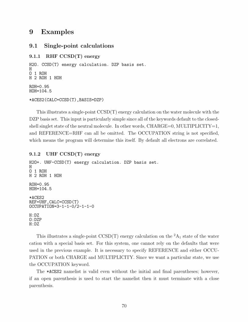
9 Examples
9.1 Single-point calculations
9.1.1 RHF CCSD(T) energy
H2O. CCSD(T) energy calculation. DZP basis set.HO 1 ROHH 2 ROH 1 HOH
ROH=0.95HOH=104.5
*ACES2(CALC=CCSD(T),BASIS=DZP)
This illustrates a single-point CCSD(T) energy calculation on the water molecule with the
DZP basis set. This input is particularly simple since all of the keywords default to the closed-
shell singlet state of the neutral molecule. In other words, CHARGE=0, MULTIPLICITY=1,
and REFERENCE=RHF can all be omitted. The OCCUPATION string is not specified,
which means the program will determine this itself. By default all electrons are correlated.
9.1.2 UHF CCSD(T) energy
H2O+. UHF-CCSD(T) energy calculation. DZP basis set.HO 1 ROHH 2 ROH 1 HOH
ROH=0.95HOH=104.5
*ACES2REF=UHF,CALC=CCSD(T)OCCUPATION=3-1-1-0/2-1-1-0
H:DZO:DZPH:DZ
This illustrates a single-point CCSD(T) energy calculation on the 2A1 state of the water
cation with a special basis set. For this system, one cannot rely on the defaults that were
used in the previous example. It is necessary to specify REFERENCE and either OCCU-
PATION or both CHARGE and MULTIPLICITY. Since we want a particular state, we use
the OCCUPATION keyword.
The *ACES2 namelist is valid even without the initial and final parentheses; however,
if an open parenthesis is used to start the namelist then it must terminate with a close
parenthesis.
70
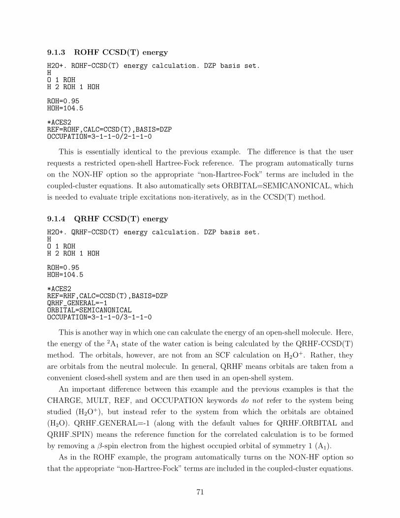
9.1.3 ROHF CCSD(T) energy
H2O+. ROHF-CCSD(T) energy calculation. DZP basis set.HO 1 ROHH 2 ROH 1 HOH
ROH=0.95HOH=104.5
*ACES2REF=ROHF,CALC=CCSD(T),BASIS=DZPOCCUPATION=3-1-1-0/2-1-1-0
This is essentially identical to the previous example. The difference is that the user
requests a restricted open-shell Hartree-Fock reference. The program automatically turns
on the NON-HF option so the appropriate “non-Hartree-Fock” terms are included in the
coupled-cluster equations. It also automatically sets ORBITAL=SEMICANONICAL, which
is needed to evaluate triple excitations non-iteratively, as in the CCSD(T) method.
9.1.4 QRHF CCSD(T) energy
H2O+. QRHF-CCSD(T) energy calculation. DZP basis set.HO 1 ROHH 2 ROH 1 HOH
ROH=0.95HOH=104.5
*ACES2REF=RHF,CALC=CCSD(T),BASIS=DZPQRHF_GENERAL=-1ORBITAL=SEMICANONICALOCCUPATION=3-1-1-0/3-1-1-0
This is another way in which one can calculate the energy of an open-shell molecule. Here,
the energy of the 2A1 state of the water cation is being calculated by the QRHF-CCSD(T)
method. The orbitals, however, are not from an SCF calculation on H2O+. Rather, they
are orbitals from the neutral molecule. In general, QRHF means orbitals are taken from a
convenient closed-shell system and are then used in an open-shell system.
An important difference between this example and the previous examples is that the
CHARGE, MULT, REF, and OCCUPATION keywords do not refer to the system being
studied (H2O+), but instead refer to the system from which the orbitals are obtained
(H2O). QRHF GENERAL=-1 (along with the default values for QRHF ORBITAL and
QRHF SPIN) means the reference function for the correlated calculation is to be formed
by removing a β-spin electron from the highest occupied orbital of symmetry 1 (A1).
As in the ROHF example, the program automatically turns on the NON-HF option so
that the appropriate “non-Hartree-Fock” terms are included in the coupled-cluster equations.
71
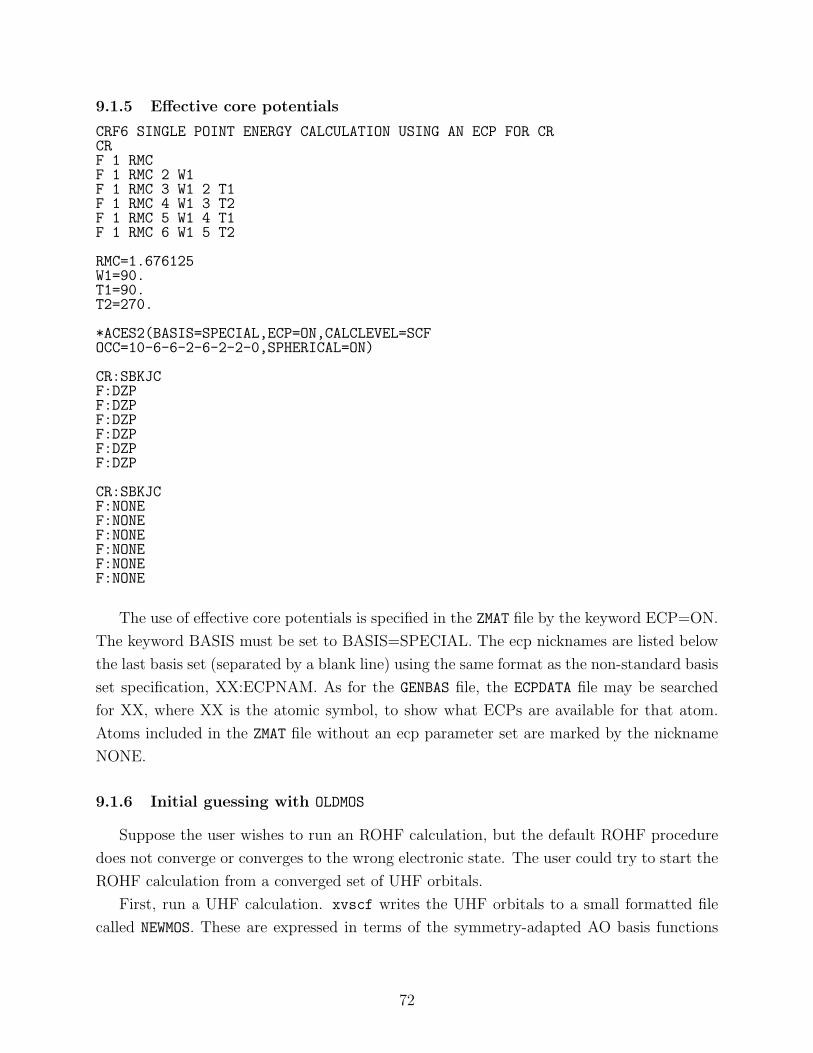
9.1.5 Effective core potentials
CRF6 SINGLE POINT ENERGY CALCULATION USING AN ECP FOR CRCRF 1 RMCF 1 RMC 2 W1F 1 RMC 3 W1 2 T1F 1 RMC 4 W1 3 T2F 1 RMC 5 W1 4 T1F 1 RMC 6 W1 5 T2
RMC=1.676125W1=90.T1=90.T2=270.
*ACES2(BASIS=SPECIAL,ECP=ON,CALCLEVEL=SCFOCC=10-6-6-2-6-2-2-0,SPHERICAL=ON)
CR:SBKJCF:DZPF:DZPF:DZPF:DZPF:DZPF:DZP
CR:SBKJCF:NONEF:NONEF:NONEF:NONEF:NONEF:NONE
The use of effective core potentials is specified in the ZMAT file by the keyword ECP=ON.
The keyword BASIS must be set to BASIS=SPECIAL. The ecp nicknames are listed below
the last basis set (separated by a blank line) using the same format as the non-standard basis
set specification, XX:ECPNAM. As for the GENBAS file, the ECPDATA file may be searched
for XX, where XX is the atomic symbol, to show what ECPs are available for that atom.
Atoms included in the ZMAT file without an ecp parameter set are marked by the nickname
NONE.
9.1.6 Initial guessing with OLDMOS
Suppose the user wishes to run an ROHF calculation, but the default ROHF procedure
does not converge or converges to the wrong electronic state. The user could try to start the
ROHF calculation from a converged set of UHF orbitals.
First, run a UHF calculation. xvscf writes the UHF orbitals to a small formatted file
called NEWMOS. These are expressed in terms of the symmetry-adapted AO basis functions
72
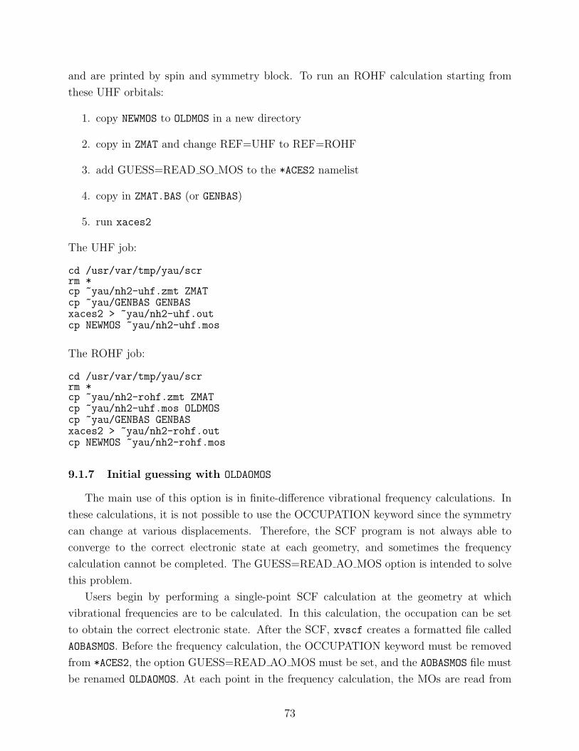
and are printed by spin and symmetry block. To run an ROHF calculation starting from
these UHF orbitals:
1. copy NEWMOS to OLDMOS in a new directory
2. copy in ZMAT and change REF=UHF to REF=ROHF
3. add GUESS=READ SO MOS to the *ACES2 namelist
4. copy in ZMAT.BAS (or GENBAS)
5. run xaces2
The UHF job:
cd /usr/var/tmp/yau/scrrm *cp ~yau/nh2-uhf.zmt ZMATcp ~yau/GENBAS GENBASxaces2 > ~yau/nh2-uhf.outcp NEWMOS ~yau/nh2-uhf.mos
The ROHF job:
cd /usr/var/tmp/yau/scrrm *cp ~yau/nh2-rohf.zmt ZMATcp ~yau/nh2-uhf.mos OLDMOScp ~yau/GENBAS GENBASxaces2 > ~yau/nh2-rohf.outcp NEWMOS ~yau/nh2-rohf.mos
9.1.7 Initial guessing with OLDAOMOS
The main use of this option is in finite-difference vibrational frequency calculations. In
these calculations, it is not possible to use the OCCUPATION keyword since the symmetry
can change at various displacements. Therefore, the SCF program is not always able to
converge to the correct electronic state at each geometry, and sometimes the frequency
calculation cannot be completed. The GUESS=READ AO MOS option is intended to solve
this problem.
Users begin by performing a single-point SCF calculation at the geometry at which
vibrational frequencies are to be calculated. In this calculation, the occupation can be set
to obtain the correct electronic state. After the SCF, xvscf creates a formatted file called
AOBASMOS. Before the frequency calculation, the OCCUPATION keyword must be removed
from *ACES2, the option GUESS=READ AO MOS must be set, and the AOBASMOS file must
be renamed OLDAOMOS. At each point in the frequency calculation, the MOs are read from
73
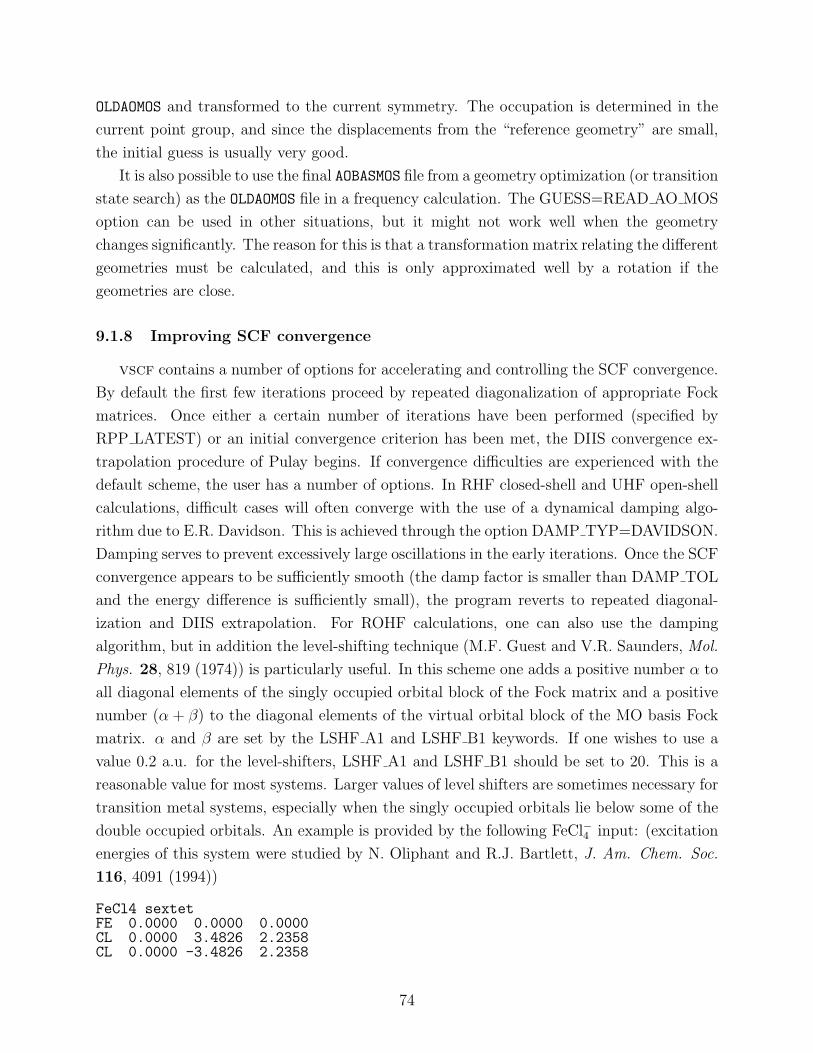
OLDAOMOS and transformed to the current symmetry. The occupation is determined in the
current point group, and since the displacements from the “reference geometry” are small,
the initial guess is usually very good.
It is also possible to use the final AOBASMOS file from a geometry optimization (or transition
state search) as the OLDAOMOS file in a frequency calculation. The GUESS=READ AO MOS
option can be used in other situations, but it might not work well when the geometry
changes significantly. The reason for this is that a transformation matrix relating the different
geometries must be calculated, and this is only approximated well by a rotation if the
geometries are close.
9.1.8 Improving SCF convergence
vscf contains a number of options for accelerating and controlling the SCF convergence.
By default the first few iterations proceed by repeated diagonalization of appropriate Fock
matrices. Once either a certain number of iterations have been performed (specified by
RPP LATEST) or an initial convergence criterion has been met, the DIIS convergence ex-
trapolation procedure of Pulay begins. If convergence difficulties are experienced with the
default scheme, the user has a number of options. In RHF closed-shell and UHF open-shell
calculations, difficult cases will often converge with the use of a dynamical damping algo-
rithm due to E.R. Davidson. This is achieved through the option DAMP TYP=DAVIDSON.
Damping serves to prevent excessively large oscillations in the early iterations. Once the SCF
convergence appears to be sufficiently smooth (the damp factor is smaller than DAMP TOL
and the energy difference is sufficiently small), the program reverts to repeated diagonal-
ization and DIIS extrapolation. For ROHF calculations, one can also use the damping
algorithm, but in addition the level-shifting technique (M.F. Guest and V.R. Saunders, Mol.
Phys. 28, 819 (1974)) is particularly useful. In this scheme one adds a positive number α to
all diagonal elements of the singly occupied orbital block of the Fock matrix and a positive
number (α + β) to the diagonal elements of the virtual orbital block of the MO basis Fock
matrix. α and β are set by the LSHF A1 and LSHF B1 keywords. If one wishes to use a
value 0.2 a.u. for the level-shifters, LSHF A1 and LSHF B1 should be set to 20. This is a
reasonable value for most systems. Larger values of level shifters are sometimes necessary for
transition metal systems, especially when the singly occupied orbitals lie below some of the
double occupied orbitals. An example is provided by the following FeCl−4 input: (excitation
energies of this system were studied by N. Oliphant and R.J. Bartlett, J. Am. Chem. Soc.
116, 4091 (1994))
FeCl4 sextetFE 0.0000 0.0000 0.0000CL 0.0000 3.4826 2.2358CL 0.0000 -3.4826 2.2358
74
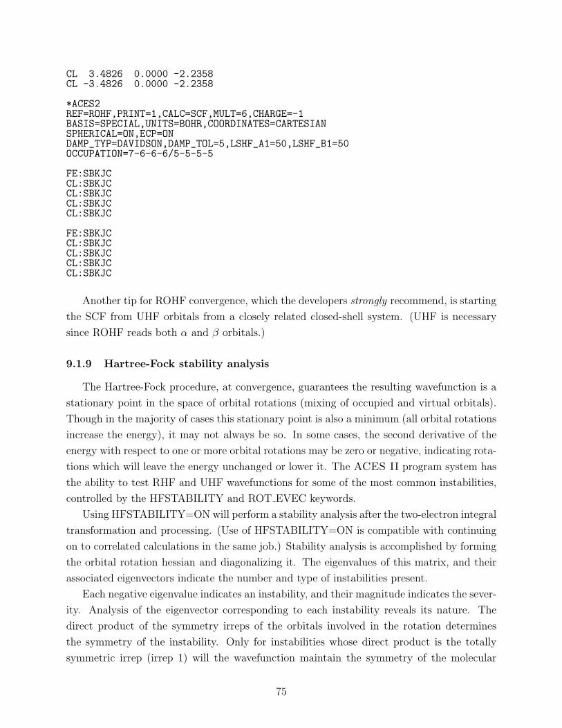
CL 3.4826 0.0000 -2.2358CL -3.4826 0.0000 -2.2358
*ACES2REF=ROHF,PRINT=1,CALC=SCF,MULT=6,CHARGE=-1BASIS=SPECIAL,UNITS=BOHR,COORDINATES=CARTESIANSPHERICAL=ON,ECP=ONDAMP_TYP=DAVIDSON,DAMP_TOL=5,LSHF_A1=50,LSHF_B1=50OCCUPATION=7-6-6-6/5-5-5-5
FE:SBKJCCL:SBKJCCL:SBKJCCL:SBKJCCL:SBKJC
FE:SBKJCCL:SBKJCCL:SBKJCCL:SBKJCCL:SBKJC
Another tip for ROHF convergence, which the developers strongly recommend, is starting
the SCF from UHF orbitals from a closely related closed-shell system. (UHF is necessary
since ROHF reads both α and β orbitals.)
9.1.9 Hartree-Fock stability analysis
The Hartree-Fock procedure, at convergence, guarantees the resulting wavefunction is a
stationary point in the space of orbital rotations (mixing of occupied and virtual orbitals).
Though in the majority of cases this stationary point is also a minimum (all orbital rotations
increase the energy), it may not always be so. In some cases, the second derivative of the
energy with respect to one or more orbital rotations may be zero or negative, indicating rota-
tions which will leave the energy unchanged or lower it. The ACES II program system has
the ability to test RHF and UHF wavefunctions for some of the most common instabilities,
controlled by the HFSTABILITY and ROT EVEC keywords.
Using HFSTABILITY=ON will perform a stability analysis after the two-electron integral
transformation and processing. (Use of HFSTABILITY=ON is compatible with continuing
on to correlated calculations in the same job.) Stability analysis is accomplished by forming
the orbital rotation hessian and diagonalizing it. The eigenvalues of this matrix, and their
associated eigenvectors indicate the number and type of instabilities present.
Each negative eigenvalue indicates an instability, and their magnitude indicates the sever-
ity. Analysis of the eigenvector corresponding to each instability reveals its nature. The
direct product of the symmetry irreps of the orbitals involved in the rotation determines
the symmetry of the instability. Only for instabilities whose direct product is the totally
symmetric irrep (irrep 1) will the wavefunction maintain the symmetry of the molecular
75
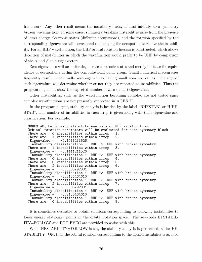
framework. Any other result means the instability leads, at least initially, to a symmetry
broken wavefunction. In some cases, symmetry breaking instabilities arise from the presence
of lower energy electronic states (different occupations), and the rotation specified by the
corresponding eigenvector will correspond to changing the occupation to relieve the instabil-
ity. For an RHF wavefunction, the UHF orbital rotation hessian is constructed, which allows
detection of instabilities in which the wavefunction would prefer to be UHF by comparison
of the α and β spin eigenvectors.
Zero eigenvalues will occur for degenerate electronic states and merely indicate the equiv-
alence of occupations within the computational point group. Small numerical inaccuracies
frequently result in nominally zero eigenvalues having small non-zero values. The sign of
such eigenvalues will determine whether or not they are reported as instabilities. Thus the
program might not show the expected number of zero (small) eigenvalues.
Other instabilities, such as the wavefunction becoming complex are not tested since
complex wavefunctions are not presently supported in ACES II.
In the program output, stability analysis is headed by the label “RHFSTAB” or “UHF-
STAB”. The number of instabilities in each irrep is given along with their eigenvalue and
classification. For example,
@RHFSTAB, Performing stability analysis of RHF wavefunction.Orbital rotation parameters will be evaluated for each symmetry block.There are 0 instabilities within irrep 1.There are 1 instabilities within irrep 2.Eigenvalue = -0.1411211526:Instability classification : RHF -> UHF with broken symmetry
There are 1 instabilities within irrep 3.Eigenvalue = -0.1411211526:Instability classification : RHF -> UHF with broken symmetry
There are 0 instabilities within irrep 4.There are 0 instabilities within irrep 5.There are 2 instabilities within irrep 6.Eigenvalue = -0.3586792381:Instability classification : RHF -> UHF with broken symmetryEigenvalue = -0.2166464610:Instability classification : RHF -> RHF with broken symmetry
There are 2 instabilities within irrep 7.Eigenvalue = -0.3586792381:Instability classification : RHF -> UHF with broken symmetryEigenvalue = -0.2166464610:Instability classification : RHF -> RHF with broken symmetry
There are 0 instabilities within irrep 8.
It is sometimes desirable to obtain solutions corresponding to following instabilities to
lower energy stationary points in the orbital rotation space. The keywords HFSTABIL-
ITY=FOLLOW and ROT EVEC are provided to assist with this.
When HFSTABILITY=FOLLOW is set, the stability analysis is performed, as for HF-
STABILITY=ON, then the orbital rotation corresponding to the chosen instability is applied
76
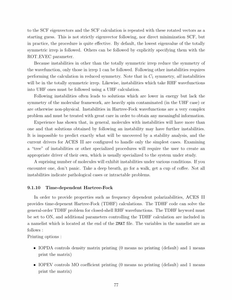
to the SCF eigenvectors and the SCF calculation is repeated with these rotated vectors as a
starting guess. This is not strictly eigenvector following, nor direct minimization SCF, but
in practice, the procedure is quite effective. By default, the lowest eigenvalue of the totally
symmetric irrep is followed. Others can be followed by explicitly specifying them with the
ROT EVEC parameter.
Because instabilities in other than the totally symmetric irrep reduce the symmetry of
the wavefunction, only those in irrep 1 can be followed. Following other instabilities requires
performing the calculation in reduced symmetry. Note that in C1 symmetry, all instabilities
will be in the totally symmetric irrep. Likewise, instabilities which take RHF wavefunctions
into UHF ones must be followed using a UHF calculation.
Following instabilities often leads to solutions which are lower in energy but lack the
symmetry of the molecular framework, are heavily spin contaminated (in the UHF case) or
are otherwise non-physical. Instabilities in Hartree-Fock wavefunctions are a very complex
problem and must be treated with great care in order to obtain any meaningful information.
Experience has shown that, in general, molecules with instabilities will have more than
one and that solutions obtained by following an instability may have further instabilities.
It is impossible to predict exactly what will be uncovered by a stability analysis, and the
current drivers for ACES II are configured to handle only the simplest cases. Examining
a “tree” of instabilities or other specialized procedures will require the user to create an
appropriate driver of their own, which is usually specialized to the system under study.
A suprising number of molecules will exhibit instabilities under various conditions. If you
encounter one, don’t panic. Take a deep breath, go for a walk, get a cup of coffee. Not all
instabilities indicate pathological cases or intractable problems.
9.1.10 Time-dependent Hartree-Fock
In order to provide properties such as frequency dependent polarizabilities, ACES II
provides time-depenent Hartree-Fock (TDHF) calculations. The TDHF code can solve the
general-order TDHF problem for closed-shell RHF wavefunctions. The TDHF keyword must
be set to ON, and additional parameters controlling the TDHF calculation are included in
a namelist which is located at the end of the ZMAT file. The variables in the namelist are as
follows :
Printing options :
• IOPDA controls density matrix printing (0 means no printing (default) and 1 means
print the matrix)
• IOPEV controls MO coefficient printing (0 means no printing (default) and 1 means
print the matrix)
77
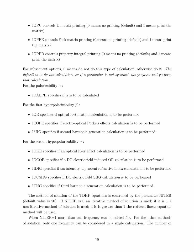
• IOPU controls U matrix printing (0 means no printing (default) and 1 means print the
matrix)
• IOPFE controls Fock matrix printing (0 means no printing (default) and 1 means print
the matrix)
• IOPPR controls property integral printing (0 means no printing (default) and 1 means
print the matrix)
For subsequent options, 0 means do not do this type of calculation, otherwise do it. The
default is to do the calculation, so if a parameter is not specified, the program will perform
that calculation.
For the polarizability α :
• IDALPH specifies if α is to be calculated
For the first hyperpolarizability β :
• IOR specifies if optical rectification calculation is to be performed
• IEOPE specifies if electro-optical Pockels effects calculation is to be performed
• ISHG specifies if second harmonic generation calculation is to be performed
For the second hyperpolarizability γ :
• IOKE specifies if an optical Kerr effect calculation is to be performed
• IDCOR specifies if a DC electric field induced OR calculation is to be performed
• IIDRI specifies if am intensity dependent refractive index calculation is to be performed
• IDCSHG specifies if DC electric field SHG calculation is to be performed
• ITHG specifies if third harmonic generation calculation is to be performed
The method of solution of the TDHF equations is controlled by the parameter NITER
(default value is 20). If NITER is 0 an iterative method of solution is used; if it is 1 a
non-iterative method of solution is used; if it is greater than 1 the reduced linear equation
method will be used.
When NITER=1 more than one frequency can be solved for. For the other methods
of solution, only one frequency can be considered in a single calculation. The number of
78
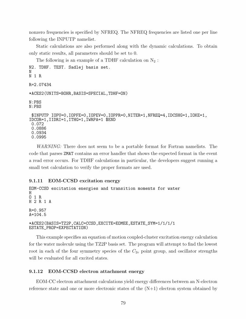
nonzero frequencies is specified by NFREQ. The NFREQ frequencies are listed one per line
following the INPUTP namelist.
Static calculations are also performed along with the dynamic calculations. To obtain
only static results, all parameters should be set to 0.
The following is an example of a TDHF calculation on N2 :
N2. TDHF. TEST. Sadlej basis set.NN 1 R
R=2.07434
*ACES2(UNITS=BOHR,BASIS=SPECIAL,TDHF=ON)
N:PBSN:PBS
$INPUTP IOPU=0,IOPFE=0,IOPEV=0,IOPPR=0,NITER=1,NFREQ=4,IDCSHG=1,IOKE=1,IDCOR=1,IIDRI=1,ITHG=1,IWRPA=1 $END0.0720.08860.09340.0995
WARNING: There does not seem to be a portable format for Fortran namelists. The
code that parses ZMAT contains an error handler that shows the expected format in the event
a read error occurs. For TDHF calculations in particular, the developers suggest running a
small test calculation to verify the proper formats are used.
9.1.11 EOM-CCSD excitation energy
EOM-CCSD excitation energies and transition moments for waterHO 1 RH 2 R 1 A
R=0.957A=104.5
*ACES2(BASIS=TZ2P,CALC=CCSD,EXCITE=EOMEE,ESTATE_SYM=1/1/1/1ESTATE_PROP=EXPECTATION)
This example specifies an equation of motion coupled-cluster excitation energy calculation
for the water molecule using the TZ2P basis set. The program will attempt to find the lowest
root in each of the four symmetry species of the C2v point group, and oscillator strengths
will be evaluated for all excited states.
9.1.12 EOM-CCSD electron attachment energy
EOM-CC electron attachment calculations yield energy differences between an N-electron
reference state and one or more electronic states of the (N+1) electron system obtained by
79
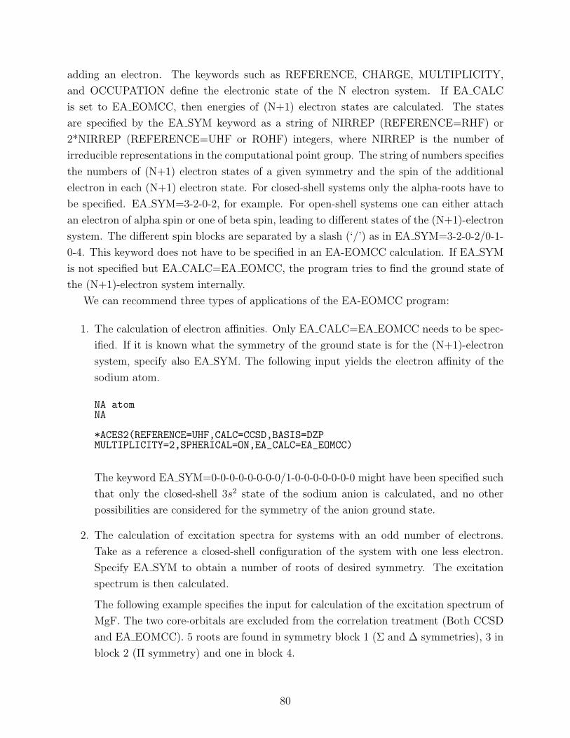
adding an electron. The keywords such as REFERENCE, CHARGE, MULTIPLICITY,
and OCCUPATION define the electronic state of the N electron system. If EA CALC
is set to EA EOMCC, then energies of (N+1) electron states are calculated. The states
are specified by the EA SYM keyword as a string of NIRREP (REFERENCE=RHF) or
2*NIRREP (REFERENCE=UHF or ROHF) integers, where NIRREP is the number of
irreducible representations in the computational point group. The string of numbers specifies
the numbers of (N+1) electron states of a given symmetry and the spin of the additional
electron in each (N+1) electron state. For closed-shell systems only the alpha-roots have to
be specified. EA SYM=3-2-0-2, for example. For open-shell systems one can either attach
an electron of alpha spin or one of beta spin, leading to different states of the (N+1)-electron
system. The different spin blocks are separated by a slash (‘/’) as in EA SYM=3-2-0-2/0-1-
0-4. This keyword does not have to be specified in an EA-EOMCC calculation. If EA SYM
is not specified but EA CALC=EA EOMCC, the program tries to find the ground state of
the (N+1)-electron system internally.
We can recommend three types of applications of the EA-EOMCC program:
1. The calculation of electron affinities. Only EA CALC=EA EOMCC needs to be spec-
ified. If it is known what the symmetry of the ground state is for the (N+1)-electron
system, specify also EA SYM. The following input yields the electron affinity of the
sodium atom.
NA atomNA
*ACES2(REFERENCE=UHF,CALC=CCSD,BASIS=DZPMULTIPLICITY=2,SPHERICAL=ON,EA_CALC=EA_EOMCC)
The keyword EA SYM=0-0-0-0-0-0-0-0/1-0-0-0-0-0-0-0 might have been specified such
that only the closed-shell 3s2 state of the sodium anion is calculated, and no other
possibilities are considered for the symmetry of the anion ground state.
2. The calculation of excitation spectra for systems with an odd number of electrons.
Take as a reference a closed-shell configuration of the system with one less electron.
Specify EA SYM to obtain a number of roots of desired symmetry. The excitation
spectrum is then calculated.
The following example specifies the input for calculation of the excitation spectrum of
MgF. The two core-orbitals are excluded from the correlation treatment (Both CCSD
and EA EOMCC). 5 roots are found in symmetry block 1 (Σ and ∆ symmetries), 3 in
block 2 (Π symmetry) and one in block 4.
80
MgF Excitation SpectrumMGF 1 R
R = 1.752
*ACES2(REFERENCE=RHF,CALC=CCSD,BASIS=TZ2P,CHARGE=1MULT=1,SPHERICAL=ON,DROPMO=1-2,EA_CALC=EA_EOMCC EA_SYM=5-3-0-1)
3. The calculation of high spin triplet states for systems with a closed-shell ground state.
Take as a CC reference the high spin doublet ground state of the positive ion, and
add an extra alpha electron by specifying EA SYM (e.g., EA SYM=4-3-0-2/0-0-0-0).
This yields high spin triplet excited states of the neutral. In addition the closed-shell
ground state can be obtained by adding a beta electron to the proper symmetry-block
(e.g., EA SYM=4-3-0-2/1-0-0-0). This has the advantage that the proper excitation
energies of the system are tabulated by the program. We note that singlet and low spin
triplet excited state energies can also be obtained by adding a beta electron. However
such calculations do not yield satisfactory results, due to spin contamination of the
resulting EA EOMCC states.
The following input yields triplet excited states for the beryllium atom. The SCF
calculation is on the closed-shell neutral system, while the QRHF option is used to
create the positive Be ion.
BE Atom Excitation spectrum, QRHF ReferenceBE
*ACES2(REFERENCE=RHF,CALC=CCSD,BASIS=SPECIALSPHERICAL=ON,QRHF_G=(-1),EA_CALC=EA_EOMCCEA_SYM=8-4-0-4-0-0-0-0/0-0-0-0-0-0-0-0)
BE:WMR
WARNING: In all EOMCC calculations it is highly recommended that the reference
state transforms according to a one-dimensional representation of the true molecular
point group. Otherwise, the likely outcome is inaccurate results, which in addition are
very hard to interpret due to a breaking of the symmetry in such a calculation.
9.1.13 NMR chemical shifts
NMR spectroscopy is a very important analytical tool for the identification and charac-
terization of molecules. However, since there is no simple correlation between the measured
chemical shifts and structural parameters, the interpretation of experimental NMR spectra
is not trivial and can be in many cases quite involved. The ability to calculate NMR chem-
ical shifts ab initio is therefore a very important advancement in quantum chemistry. The
81
calculation of chemical shifts can provide in many cases the necessary information for the
correct interpretation of experimental NMR spectra. Therefore, methods for the computa-
tion of NMR chemical shifts at SCF and correlated levels (currently limited to MBPT(2))
have been added in the last years to the functionalities of the ACES II program system.
However, before discussing the details of the calculation of NMR chemical shifts, a few
general remarks are required. The main problem in all calculations of magnetic properties
(i.e., NMR chemical shifts and magnetizabilities) using finite basis sets (as they are usually
employed in quantum chemical calculations) is the gauge-invariance problem. This simply
means that the results of such a calculation depend on the chosen gauge-origin and are
not invariant with respect to gauge transformations as required by exact theory. A trivial
solution to the gauge-invariance problem would be the use of very large basis sets in order to
minimize the gauge error, but this approach, due to large computational costs, is limited to
small molecules. More satisfying solutions are offered by approaches which introduce local
gauge-origins to define the vector potential such as the IGLO method of Kutzelnigg and
Schindler, the LORG method of Hansen and Bouman and the GIAO-approach of Ditchfield.
The latter originates in London’s work on molecular diamagnetism in the thirties and was
first used by Hameka during the sixties to calculate magnetizabilities and chemical shieldings.
ACES II incorporates the GIAO-SCF and GIAO-MBPT(2) method for calculating chemical
shifts, since in our opinion, the GIAO approach is the most elegant solution to the gauge-
invariance problem and in contrast to the IGLO method, is easily extended to correlated
approaches (as for example in the GIAO-MBPT(2) method).
The calculation of NMR chemical shifts are invoked via the keyword PROP=NMR to-
gether with the appropriate specification of the quantum chemical method (CALC=SCF
gives then GIAO-SCF, CALC=MBPT(2) gives GIAO-MBPT(2)). In principle, no other op-
tion is required to run calculations of NMR chemical shifts. However, to ensure the success
of GIAO-MBPT(2) calculations and in particular large-scale calculations with the GIAO-
MBPT(2) method, the computational requirements of such calculations should be kept in
mind. While CPU requirements are of less interest (a GIAO-MBPT(2) calculation is in terms
of the CPU usually less expensive than the corresponding MBPT(2) geometry optimization),
memory and disk space requirements are of special concern. The memory requirements are
for the xnmr module approximately 2 ∗ n2N2/h2 eight byte words with n denoting the num-
ber of occupied orbitals, N denoting the number of virtual orbitals, and h specifying the
order of the molecular point group. However, the current memory bottleneck is the integral
sorting in the module xintprc which requires roughly 2∗n2N2/h eight byte words and which
therefore is more demanding. The disk space requirement of a GIAO-MBPT(2) calculation
is for most parts determined by the fact that the current version depends on the storage
of the GIAO integrals. To summarize the necessary resources, a GIAO-MBPT(2) calcula-
82
tions requires the storage of the AO two-electron integrals (files IIII, IIJJ, IJIJ, and IJKL
depending on symmetry and with a total size of approximately 1.5 ∗ N4basis/(8h) eight byte
words (note that the CRAY version requires 2 ∗ N4basis/(8h) words), the storage of the MO
integrals (file MOINTS, the largest portion is here given by the integrals 〈ab||ci〉 with a total
size nN3/h eight byte words), the storage of the GIAO integrals (files IIIIX, IIJJX, IJIJX,
IJKLX in case of a symmetric perturbation Bx or IIIJX, IJIKX, IJKLX for a non-symmetric
perturbation Bx. The files for the perturbations By and Bx are named using the same
convention with Y or Z instead of X. The total size of these files is for each perturbation
approximately given by 1.5∗N4basis/(4h) (CRAY version : 2∗N4
basis/(4h))), and the storage of
the derivative MO integrals and amplitudes (files DERGAM and DERINT with the largest
portion given by the perturbed 〈ab||ci〉 integrals (size nN3/h eight byte words)). To keep
the disk space requirements at a minimum, it is strongly recommended to use the keyword
TREAT PERTURBATION=SEQUENTIAL, as this forces the program to treat each mag-
netic field component separately and thus requires only the storage of one type of GIAO
integrals at one time. TREAT PERTURBATION=SIMULTANEOUS (which is currently
the default) requires the simultaneous storage of all GIAO-integrals and is therefore much
more demanding in terms of disk space, though more efficient with respect to CPU timings.
The current limits for GIAO-MBPT(2) calculations depend on the available hardware
resources. However, as a rough guide the limits for a IBM RS6000/350 work station with 80
Mbyte memory and 3.5 Gbyte scratch space are given. Within this environment, calculations
with about 250 basis functions in D2h symmetry, about 200 basis functions in C2v, C2h, and
D2 symmetry, about 170 basis functions in C2, Ci, and Cs-symmetry and about 130 basis
functions in cases without symmetry are feasible. From these estimates it is seen that the
limits strongly depend on the molecular symmetry. Thus, users are urged to use symmetry
whenever possible. It should be also noted that the computational requirements depend
somewhat on the ratio n/N and that the costs increases with the number of occupied orbitals.
As the final result the corresponding chemical shielding tensors of all nuclei in the
molecule are obtained in a GIAO-SCF and/or GIAO-MBPT(2) calculation. The output
produced by the module xjoda gives the absolute isotropic shielding (one third of the trace
of the shielding tensor) as well as the anisotropic shielding which is usually of less interest.
In order to compare with experimental results, the absolute shielding σ must be converted
to the relative shifts δ. This is easily accomplished via
δ = σref − σ (1)
with σref as the absolute shielding of the chosen reference compounds. For 13C, tetram-
ethylsilane (TMS) has been chosen as standard and the corresponding σ values are 198.944
(dzp/dz), 193.103 (tzp/dz), 193.419 (tzp/dzp) at GIAO-SCF level and 205.720 (dzp/dz),
83
198.890 (tzp/dz), and 197.191 (tzp/dzp) at GIAO-MBPT(2) level. The MBPT(2)/6-31G*
optimized geometry has been used in all the GIAO calculations for TMS.
With respect to basis sets, the following recommendations can be made. In case of 11B
and 13C – nuclei which have been extensively studied – the dzp/dz basis set (dzp for C
and dz for H) is in most cases sufficient for relative shifts, though the use of the tzp/dz
basis (tzp for C and dz for H) is recommended. Larger basis sets (i.e., tzp, tzp2, or even
qz2p) are in most cases not needed for the accurate prediction of chemical shifts. On the
other side, 15N, 17O, and 19F NMR chemical shift calculations require larger basis sets of at
least triple-zeta plus polarization quality. Though qualitatively good results are obtained in
many cases with the tzp basis, even larger basis sets such as tz2p or qz2p are recommended
for more reliable calculations. For other nuclei, not very much can be said at the moment
and the user is strongly urged to check carefully the basis set dependence to ensure reliable
theoretical results. However, limited experience suggests that for second-row elements quite
large basis sets are needed for accurate calculations.
Note : NMR chemical shift calculations can currently only be performed with Cartesian
basis functions—SPHERICAL=ON may not be specified.
GIAO-MBPT(2) NMR chemical shift calculations for the benzonium cationC 0.000000 0.000000 -1.393615C 0.000000 0.000000 1.413386C 0.000000 -1.250334 -0.632255C 0.000000 1.250334 -0.632255C 0.000000 -1.237545 0.742530C 0.000000 1.237545 0.742530H 0.853412 0.000000 -2.102274H -0.853412 0.000000 -2.102274H 0.000000 -2.189398 -1.180688H 0.000000 2.189398 -1.180688H 0.000000 -2.161755 1.310996H 0.000000 2.161755 1.310996H 0.000000 0.000000 2.502007
*ACES2(CALC=MBPT(2),PROP=NMR,CHARGE=1COORD=CARTESIAN,TREAT_PERTURBATION=SEQUENTIAL,MEMORY=24000000)
C:DZPC:DZPC:DZPC:DZPC:DZPC:DZPH:DZH:DZH:DZH:DZH:DZH:DZH:DZ
This example features a calculation of the NMR chemical shifts at the MBPT(2) level
84
using gauge-including atomic orbitals (GIAOs). NMR shifts are requested by the keyword
PROP=NMR. The input of the coordinates in this example is via Cartesian coordinates (in
Angstroms) and the basis set is specified via the non-standard input which allows the use
of different basis sets for different atoms (in this case, DZP for C and DZ for H). To reduce
disk space requirements, the keyword TREAT PERTUBATION=SEQUENTIAL is specified
which forces the program to treat each magnetic field perturbation separately, thus storing
only GIAO integrals of one particular type at one time. The memory requirement in this
example is set to 24000000 integer-words (91.5MB on 32-bit builds and 183.1MB on 64-bit
builds).
9.2 Geometry optimizations
9.2.1 Full optimization of internal coordinates
H2O. CCSD optimization.HO 1 ROH*H 2 ROH* 1 HOH*
ROH=0.95HOH=104.5
*ACES2(CALC=CCSD,BASIS=DZP)
This specifies a geometry optimization of the water molecule with the CCSD method and
the DZP basis set. The input is exactly the same as the RHF single-point energy example,
except that an asterisk (∗) is placed after each variable to be optimized (both bond lengths
and the bond angle). Since all of the parameters are being optimized, it is also sufficient to
use GEOM OPT=FULL and leave the asterisks out of the Z matrix.
Defaults for all of the optimization keywords (e.g., METHOD and CONVERGENCE)
are used. The presence of the asterisks promotes the GEOM OPT keyword from NONE to
PARTIAL, which turns on all appropriate derivative keywords. Geometry optimizations by
default are performed using analytical gradients. If analytical gradients are not available,
one can do geometry optimizations from energies using GRAD CALC=NUMERICAL.
9.2.2 Partial optimization of internal coordinates
Beryllium borohydride, D3d structure, geometry optimization.XBE 1 R1B 2 R* 1 AB 2 R* 1 A 3 TX 2 RX* 1 A 3 TX 2 RX* 1 A 4 TH 5 RHX* 2 A 1 TH 5 RHX* 2 A 1 T60
85
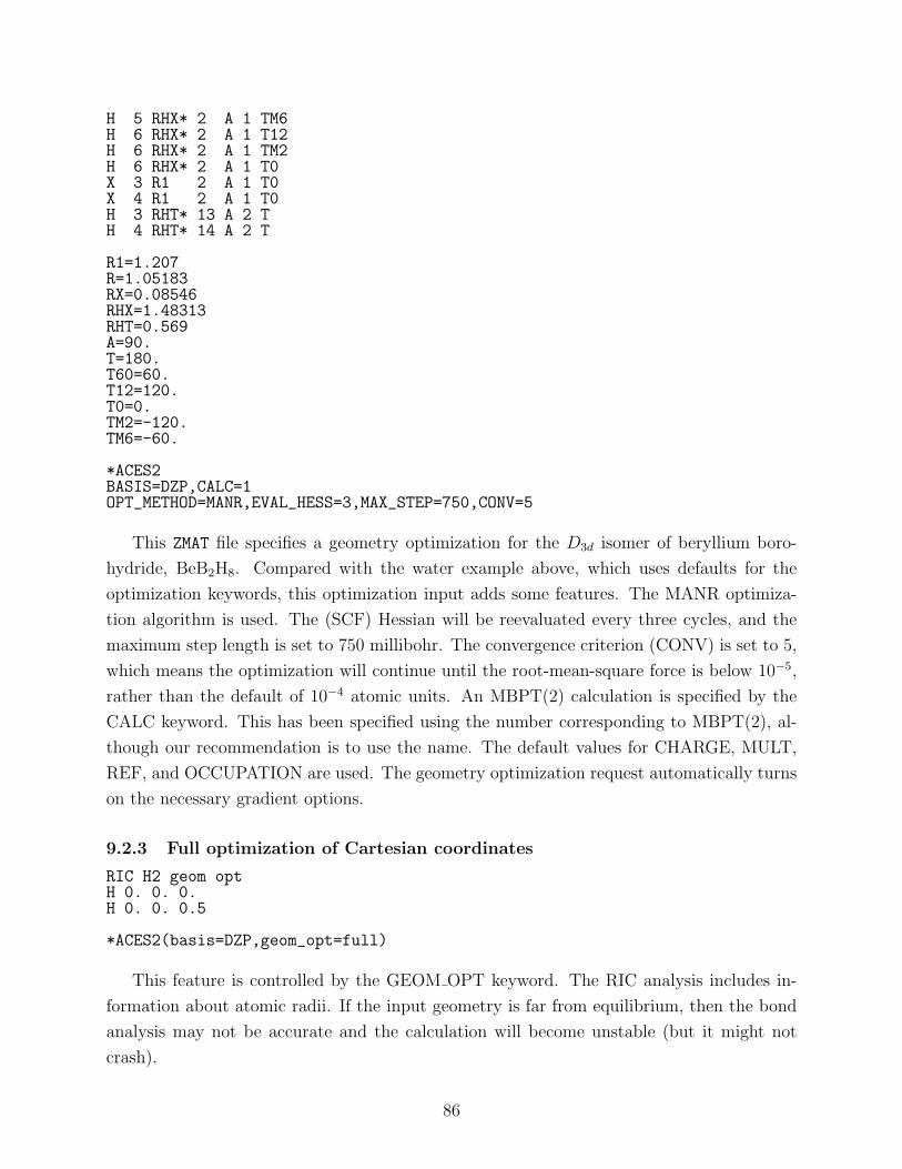
H 5 RHX* 2 A 1 TM6H 6 RHX* 2 A 1 T12H 6 RHX* 2 A 1 TM2H 6 RHX* 2 A 1 T0X 3 R1 2 A 1 T0X 4 R1 2 A 1 T0H 3 RHT* 13 A 2 TH 4 RHT* 14 A 2 T
R1=1.207R=1.05183RX=0.08546RHX=1.48313RHT=0.569A=90.T=180.T60=60.T12=120.T0=0.TM2=-120.TM6=-60.
*ACES2BASIS=DZP,CALC=1OPT_METHOD=MANR,EVAL_HESS=3,MAX_STEP=750,CONV=5
This ZMAT file specifies a geometry optimization for the D3d isomer of beryllium boro-
hydride, BeB2H8. Compared with the water example above, which uses defaults for the
optimization keywords, this optimization input adds some features. The MANR optimiza-
tion algorithm is used. The (SCF) Hessian will be reevaluated every three cycles, and the
maximum step length is set to 750 millibohr. The convergence criterion (CONV) is set to 5,
which means the optimization will continue until the root-mean-square force is below 10−5,
rather than the default of 10−4 atomic units. An MBPT(2) calculation is specified by the
CALC keyword. This has been specified using the number corresponding to MBPT(2), al-
though our recommendation is to use the name. The default values for CHARGE, MULT,
REF, and OCCUPATION are used. The geometry optimization request automatically turns
on the necessary gradient options.
9.2.3 Full optimization of Cartesian coordinates
RIC H2 geom optH 0. 0. 0.H 0. 0. 0.5
*ACES2(basis=DZP,geom_opt=full)
This feature is controlled by the GEOM OPT keyword. The RIC analysis includes in-
formation about atomic radii. If the input geometry is far from equilibrium, then the bond
analysis may not be accurate and the calculation will become unstable (but it might not
crash).
86
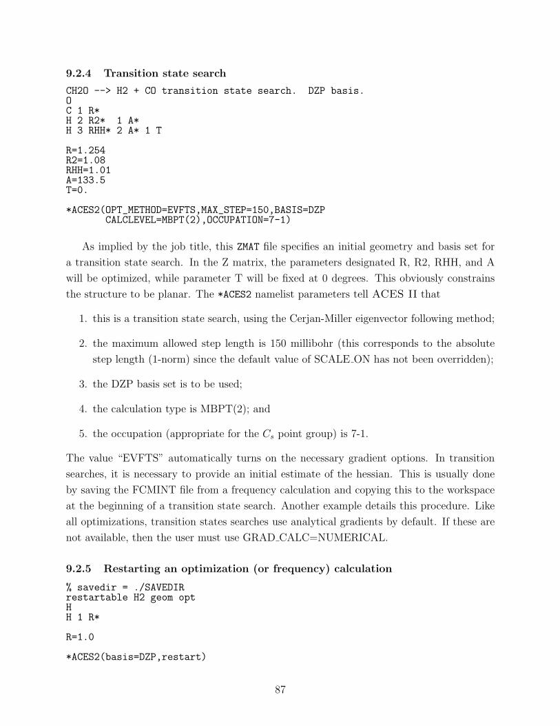
9.2.4 Transition state search
CH2O --> H2 + CO transition state search. DZP basis.OC 1 R*H 2 R2* 1 A*H 3 RHH* 2 A* 1 T
R=1.254R2=1.08RHH=1.01A=133.5T=0.
*ACES2(OPT_METHOD=EVFTS,MAX_STEP=150,BASIS=DZPCALCLEVEL=MBPT(2),OCCUPATION=7-1)
As implied by the job title, this ZMAT file specifies an initial geometry and basis set for
a transition state search. In the Z matrix, the parameters designated R, R2, RHH, and A
will be optimized, while parameter T will be fixed at 0 degrees. This obviously constrains
the structure to be planar. The *ACES2 namelist parameters tell ACES II that
1. this is a transition state search, using the Cerjan-Miller eigenvector following method;
2. the maximum allowed step length is 150 millibohr (this corresponds to the absolute
step length (1-norm) since the default value of SCALE ON has not been overridden);
3. the DZP basis set is to be used;
4. the calculation type is MBPT(2); and
5. the occupation (appropriate for the Cs point group) is 7-1.
The value “EVFTS” automatically turns on the necessary gradient options. In transition
searches, it is necessary to provide an initial estimate of the hessian. This is usually done
by saving the FCMINT file from a frequency calculation and copying this to the workspace
at the beginning of a transition state search. Another example details this procedure. Like
all optimizations, transition states searches use analytical gradients by default. If these are
not available, then the user must use GRAD CALC=NUMERICAL.
9.2.5 Restarting an optimization (or frequency) calculation
% savedir = ./SAVEDIRrestartable H2 geom optHH 1 R*
R=1.0
*ACES2(basis=DZP,restart)
87
This example reinforces the default restart behavior. If restarting the calculation is not
necessary, then use RESTART=OFF or !RESTART in the *ACES2 namelist. All of the restart
capability is built into xjoda and is controlled by two values: the SAVEDIR directive and the
RESTART flag. The SAVEDIR directive is case insensitive, and the path may be absolute
or relative. Each time xjoda is called, it copies the optimization history files to SAVEDIR.
If xjoda is called and the files are contaminated, meaning the previous job was interrupted
(or the dirty flag was not cleared), then it will restore the history files from SAVEDIR and
continue on as if nothing had happened. This applies to both geometry optimizations and
VIB=FINDIF frequency calculations.
WARNING: Restarts are only implemented for coarse-grain checkpointing. If other
ACES II files are in the directory, interesting things might happen. For the best results,
calculations should be restarted from a clean directory (i.e., only the original user input files
should be present).
When the optimization is finished, xjoda will delete the CURRENT and OLD directories
within SAVEDIR but will not delete that top-level directory. (This behavior might change in
that if xjoda created SAVEDIR, then it will delete it as well.)
9.2.6 Initializing the Hessian with FCMINT in a geometry search
All of the geometry optimization algorithms incorporated into ACES II are based on
the Newton-Raphson method, in which step directions and sizes are related to the first and
second derivatives of the molecular potential energy. However, in almost all practical calcu-
lations the exact second derivative matrix is not evaluated but rather approximated. As the
calculation progresses, well-established numerical methods are used to estimate the elements
of the Hessian matrix based on all previous optimization steps. After a large number of steps
have been taken, one may safely assume that the totally symmetric Hessian used to form the
step is a reasonable approximation to the correct Hessian. However, in the early stages of the
optimization there is not a sufficient amount of available information to accurately estimate
the Hessian and problems may ensue. By default, ACES II geometry optimizations begin
with a very crude estimate of the Hessian in which all force constants for bonded interac-
tions (as specified by the Z matrix connectivity) are set to 1 hartree/bohr2, all bending force
constants (corresponding to bond angles in the Z matrix) are set to 0.25 hartree/bohr2, and
all torsional force constants are set to 0.10 hartree/bohr2. While this initialization and the
subsequent numerical updates work satisfactorily for most small molecules, there can be oc-
casional problems. In these cases, one might wish to use an alternative initial force constant
matrix, particularly one obtained by ACES II at the same or another level of theory. There
are a number of ways in which one might do this. First, the EVAL HESS keyword can be
used. If nonzero, the value associated with this keyword directs ACES II to calculate the
88
SCF Hessian matrix prior to the first optimization step and then every N steps thereafter,
where N is the value of EVAL HESS. By setting N to a sufficiently large value (larger than
OPT MAXCYC), then the Hessian will never be recalculated and the optimization will begin
with the SCF Hessian.
However, the strategy based on EVAL HESS is not sufficient for all purposes. For ex-
ample, one might wish to use a Hessian which is evaluated at the correlated level. This
is not possible with EVAL HESS, since it will direct ACES II to calculate only the SCF
Hessian, regardless of the calculation type. Alternatively, one might adopt the economi-
cal strategy of using a Hessian which is evaluated at a low level of theory, such as SCF
with the STO-3G basis set. This is the recommended approach for transition state searches
and all optimizations for which the default Hessian is inadequate. In any event, it is quite
straightforward to use another set of force constants to begin an optimization. First, one
simply runs a harmonic frequency calculation at the desired level of theory and saves the
file named FCMINT. This formatted file contains the full internal coordinate force constant
matrix. When xjoda performs a geometry optimization, it checks the active working area
for the presence of FCMINT—no special keywords or commands are needed to do this. If the
file exists, xjoda uses those force constants to initialize the Hessian matrix.
While the geometry (and even the point group symmetry) specified by ZMAT in the har-
monic frequency calculation need not be the same as that used in the first step of the
geometry optimization, the Z matrix connectivity must be identical. If one attempts to use
an entirely different Z matrix, then the definitions of internal coordinates are no longer the
same and chaos may ensue. While this point may seem to be unimportant, this situation
occurs relatively frequently. Suppose the equilibrium geometry for a transition state is as-
sumed to be planar, and the user attempts to locate a stationary point. However, when the
harmonic frequencies are calculated, two modes are found to have imaginary frequencies:
an a′ mode (in-plane) and an a′′ mode, with the a′ mode corresponding (approximately) to
the reaction coordinate of interest. As a result, the true transition state geometry does not
contain a plane of symmetry and another search must be performed in a reduced symmetry.
To this end, it would certainly be useful to use FCMINT obtained in the frequency calculation
to start the search, but one must be careful that the molecular configuration used in the
reduced symmetry has exactly the same connectivity scheme as that used in the search for
the planar structure.
9.3 Frequency calculations
9.3.1 Numerical frequencies from analytical gradients
N4 finite difference frequency calculationN
89
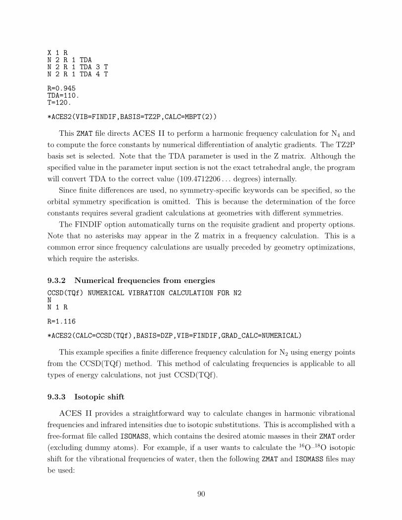
X 1 RN 2 R 1 TDAN 2 R 1 TDA 3 TN 2 R 1 TDA 4 T
R=0.945TDA=110.T=120.
*ACES2(VIB=FINDIF,BASIS=TZ2P,CALC=MBPT(2))
This ZMAT file directs ACES II to perform a harmonic frequency calculation for N4 and
to compute the force constants by numerical differentiation of analytic gradients. The TZ2P
basis set is selected. Note that the TDA parameter is used in the Z matrix. Although the
specified value in the parameter input section is not the exact tetrahedral angle, the program
will convert TDA to the correct value (109.4712206 . . . degrees) internally.
Since finite differences are used, no symmetry-specific keywords can be specified, so the
orbital symmetry specification is omitted. This is because the determination of the force
constants requires several gradient calculations at geometries with different symmetries.
The FINDIF option automatically turns on the requisite gradient and property options.
Note that no asterisks may appear in the Z matrix in a frequency calculation. This is a
common error since frequency calculations are usually preceded by geometry optimizations,
which require the asterisks.
9.3.2 Numerical frequencies from energies
CCSD(TQf) NUMERICAL VIBRATION CALCULATION FOR N2NN 1 R
R=1.116
*ACES2(CALC=CCSD(TQf),BASIS=DZP,VIB=FINDIF,GRAD_CALC=NUMERICAL)
This example specifies a finite difference frequency calculation for N2 using energy points
from the CCSD(TQf) method. This method of calculating frequencies is applicable to all
types of energy calculations, not just CCSD(TQf).
9.3.3 Isotopic shift
ACES II provides a straightforward way to calculate changes in harmonic vibrational
frequencies and infrared intensities due to isotopic substitutions. This is accomplished with a
free-format file called ISOMASS, which contains the desired atomic masses in their ZMAT order
(excluding dummy atoms). For example, if a user wants to calculate the 16O–18O isotopic
shift for the vibrational frequencies of water, then the following ZMAT and ISOMASS files may
be used:
90
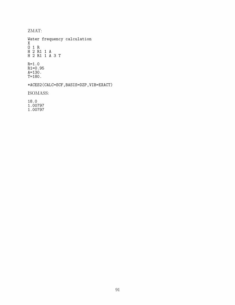
ZMAT:
Water frequency calculationXO 1 RH 2 R1 1 AH 2 R1 1 A 3 T
R=1.0R1=0.95A=130.T=180.
*ACES2(CALC=SCF,BASIS=DZP,VIB=EXACT)
ISOMASS:
18.01.007971.00797
91
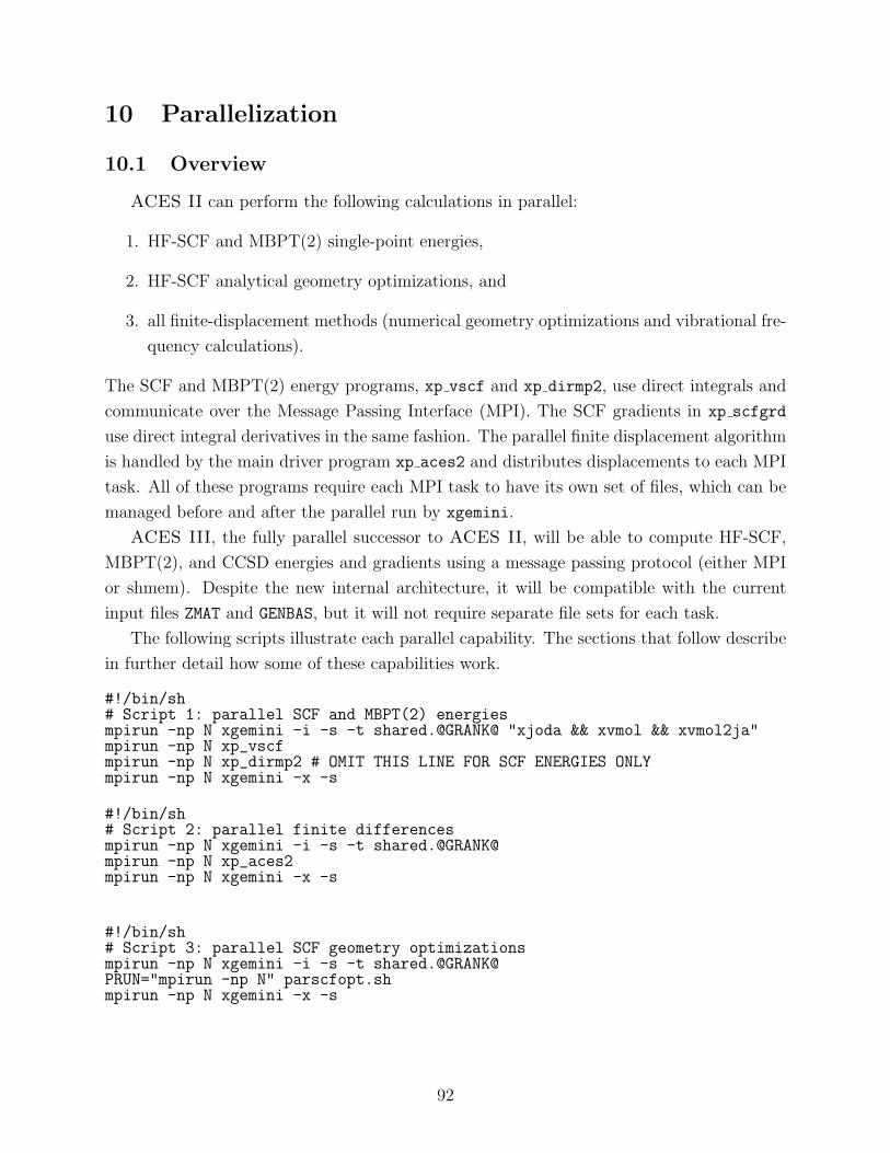
10 Parallelization
10.1 Overview
ACES II can perform the following calculations in parallel:
1. HF-SCF and MBPT(2) single-point energies,
2. HF-SCF analytical geometry optimizations, and
3. all finite-displacement methods (numerical geometry optimizations and vibrational fre-
quency calculations).
The SCF and MBPT(2) energy programs, xp vscf and xp dirmp2, use direct integrals and
communicate over the Message Passing Interface (MPI). The SCF gradients in xp scfgrd
use direct integral derivatives in the same fashion. The parallel finite displacement algorithm
is handled by the main driver program xp aces2 and distributes displacements to each MPI
task. All of these programs require each MPI task to have its own set of files, which can be
managed before and after the parallel run by xgemini.
ACES III, the fully parallel successor to ACES II, will be able to compute HF-SCF,
MBPT(2), and CCSD energies and gradients using a message passing protocol (either MPI
or shmem). Despite the new internal architecture, it will be compatible with the current
input files ZMAT and GENBAS, but it will not require separate file sets for each task.
The following scripts illustrate each parallel capability. The sections that follow describe
in further detail how some of these capabilities work.
#!/bin/sh# Script 1: parallel SCF and MBPT(2) energiesmpirun -np N xgemini -i -s -t shared.@GRANK@ "xjoda && xvmol && xvmol2ja"mpirun -np N xp_vscfmpirun -np N xp_dirmp2 # OMIT THIS LINE FOR SCF ENERGIES ONLYmpirun -np N xgemini -x -s
#!/bin/sh# Script 2: parallel finite differencesmpirun -np N xgemini -i -s -t shared.@GRANK@mpirun -np N xp_aces2mpirun -np N xgemini -x -s
#!/bin/sh# Script 3: parallel SCF geometry optimizationsmpirun -np N xgemini -i -s -t shared.@GRANK@PRUN="mpirun -np N" parscfopt.shmpirun -np N xgemini -x -s
92
10.2 Running xgemini
xgemini is a tool for managing private scratch directories from a central location. Each
MPI task (of xgemini or the parallel AMEs) must start in this directory, which means it
must be globally visible on distributed computers. Henceforth, this directory will be called
WORKDIR. Depending on the machine architecture, the two choices the user must make
are: (1) where will the private scratch directories be created and (2) how will the AMEs get
to them. These decisions will affect performance if local disks are available on each node
and will determine how a parallel job should be restarted.
When the user runs a parallel member executable (usually xp aces2), each parallel task
must start in WORKDIR, which usually contains ZMAT and GENBAS. Before reading any
files, each task attempts to cd into a directory called nodename.rank. The tasks on a
machine named crunch would look for “crunch.0”, “crunch.1”, etc. If they cannot find these
directories, then they try to cd into directories called shared.rank (shared.0, shared.1, etc.).
If those are not found either then the tasks start running in the current directory.
10.2.1 Local scratch directories
For the following example, assume that the parallel computer has compute nodes called
compnode0, compnode1, etc. and that the user (named smith) is allowed to create directories
in /local/tmp. The following command will create a directory called smithdir on every
node:
xgemini -i -t /local/tmp/smithdir
Assuming all compute nodes took part in the parallel run, then it is likely that the user
would see the following WORKDIR directory listing:
ZMAT GENBAS compnode0.0 compnode1.1 compnode2.2 ...
Each compnodeX.X is a symbolic link that points to /local/tmp/smithdir, and inside each
of those local directories are symbolic links back to ZMAT and GENBAS. The -i flag is what
instructs xgemini to create the directories and links.
It is usually the case that if local directory partitions are available then performing I/O on
them will yield better performance than reading and writing to a partition over the network.
The downside is that if a parallel job is stopped and needs to be restarted, then the user
must tell the parallel job scheduler (like LoadLeveler or PBS) to run the new job on the
same nodes that the previous job ran on (simply because those are the nodes with the data).
93
10.2.2 Shared scratch directories
If a global file system (like GPFS or even NFS) is used for the scratch directories, then
a task on any node can get to any other scratch directory. Assume user smith can cre-
ate directories in /global/tmp. Reusing the previous xgemini command line with “lo-
cal” changed to “global” will not work because every parallel task will attempt to create
/global/tmp/smithdir. One task will succeed but all of the others will fail (and crash).
gemini has a rich set of pattern macros for this kind of customization, but the simplest
command to use for the job would be:
xgemini -i -s -t /global/tmp/smithdir.@GRANK@
Each task will replace the string “@GRANK@” will its global rank (an integer from 0 to
N-1, where N is the number of parallel tasks).
Creating scratch directories in /global allows all nodes in the computer to see all scratch
directories, but the symbolic links in WORKDIR will still be named compnodeX.Y unless
the -s flag is used. If a parallel job is restarted, process 0 might be running on compnode2,
and it would expect to see compnode2.0 in WORKDIR. However, if the previous run had
process 0 running on compnode0, then it would have created compnode0.0, and the restarted
job will crash. With -s, the symbolic links in WORKDIR are named shared.rank, so it does
not matter which actual node created the scratch directory or the link to it. If shared links
are used, then every call to xgemini must use the -s flag. The downside to remote scratch
directories is that performance might decrease with high network traffic, although this is
highly dependent on the hardware architecture and runtime load.
Some users might feel more comfortable limiting all activity to WORKDIR. In this case,
the scratch directory pattern can be the same as the symbolic link. For example,
xgemini -i -s -t shared.@GRANK@
will create directories instead of symbolic links in WORKDIR. The parallel AMEs will not
know the difference when they attempt to cd into the scratch directory.
10.2.3 Command-line flags and pattern macros
As previously demonstrated, xgemini can create the runtime environment (with -i),
can use “shared” node names (with -s), and can create private scratch directories with
almost any name the user requires (with -t and macro substitution). In addition, it can use
arbitrary input and basis files (with -z and -b), can run serial commands in each directory
(all arguments that are not flags), and can clean up after a parallel run (with -x). The
command-line structure is as follows:
94
xgemini [-h] [-s] [-i [-z file] [-b file] [-t pattern]] [-x] [--] [exec]
Flag Description
-h print usage text
-s use shared scratch directories (useful for restarts)
-i initialize (make scratch directories and symlinks)
-z file link file to ZMAT (default is “ZMAT”)
-b file link file to GENBAS (default is “GENBAS”)
-t pattern pattern defines scratch directory paths
-x clean (remove scratch directories and symlinks)
-- terminate xgemini flag parsing
exec pass exec arguments to a system command in each scratch directory
The pattern that defines the scratch directories can be an absolute or relative path with
respect to WORKDIR. Another example of directory patterns is
/usr/var/tmp/@LOGNAME@/scr.@GRANK@
which would become
/usr/var/tmp/smith/scr.0
for the root task of user smith. The following table shows the complete list of macros and
their substituted values.
Macro Substitution
@NODENAME@ the string at uname.nodename as described by sys/utsname.h
(most likely “uname -n”)
@LOGNAME@ the string returned by getlogin r() or cuserid()
(most likely “whoami”)
@SID@ the session ID of the xgemini process
@PID@ the ID of the xgemini process
@PPID@ the ID of the xgemini parent process
@GRANK@ the MPI process rank in MPI COMM WORLD
@GPROCS@ the number of MPI processes in MPI COMM WORLD
@HRANK@ the MPI process rank in MPI COMM HOST
@HPROCS@ the number of MPI processes in MPI COMM HOST
95
10.3 Examples
10.3.1 Parallel finite differences with MPI (automatic)
The two programs that are of primary concern in this exercise are xgemini and xp aces2.
Assume xgemini creates shared scratch directories:
WORKDIR> ls
ZMAT GENBAS
WORKDIR> xgemini -i -s -t /local/tmp/smith.@GRANK@
...
WORKDIR> ls -F
ZMAT GENBAS shared.0@ shared.1@ ...
Before running xp aces2, the user should determine if output tagging is available for
parallel processes. Without this, the standard output stream of every process will be merged
and it will be almost impossible to discern which task did what. Furthermore, since the
operating system buffers I/O streams, the final lines of output might not contain the “final
answer.” IBM’s parallel environment can tag each line with the global rank if “-labelio
yes” is used (or if MP LABELIO=yes is set in the environment). (HP/Compaq computers
also have a tagging feature.)
WORKDIR> xp aces2 -labelio yes > out
...
WORKDIR> grep ‘^ *0:’ out
0: [output from task 0]
...
And finally,
WORKDIR> xgemini -x -s
...
WORKDIR> ls
ZMAT GENBAS out
The user should not request more process elements than there are finite displacements.
If this happens, then some instances of xjoda will see there are no displacements and bomb.
The surest way of checking this before submitting the job is by running xjoda on the input
file. The FD logic will print out a table like the following: (data from CH4 fully numerical
vibrational frequencies in C1)
96
@VIBINF-I, Symmetries species for nuclear motions:Irrep Label Total Vibrations Translations Rotations
1 A 15.00 9.00 3.00 3.00Total number of calculations required : 90Number of single-point energy calculations : 90Number of energy gradient calculations : 0
For frequency calculations using numerical gradients, the reference geometry is added to the
set of displacements, so the example above can be run with at most 91 process elements.
CH4 frequencies in C1 with analytical gradients (or geometry optimization with numerical
gradients) can use at most 18 process elements.
10.3.2 Parallel finite differences with scripts (manual)
Running a set of calculations in parallel by hand (i.e., without MPI) is certainly doable,
and because the synchronization is handled through ASCII files, the calculations can even
be performed on different architectures; however, it is not pretty to coordinate, and if the
user is running an optimization with numerical gradients, then he or she should expect a lot
of intervention before the coordinates converge. In addition to complicated shell scripting,
the user must also know the exact order of ACES member executables that are required for
each single point calculation.
The serial xjoda binary can accept two command-line flags, -procs and -rank, that
instruct it to set up single-point calculations on a subset of the displacements. Once the last
displacement is complete (but before the final xjoda), the user must update each local file
set with the data from all of the other file sets. For vibrational frequencies, this can be done
on a single file set, but for geometry optimizations, each file set must be updated before
taking the next step.
The two programs that are of primary concern are xjoda and xa2proc. Every time
xjoda is called, the number of processes and the rank must be supplied on the command
line. xa2proc contains a module that will update, print, and load the data needed from each
file set.
The following Korn shell script will run through every AME for every virtual process and
collate the results of a vibrational frequency calculation. This example does the same thing
as the serial xaces2 program on one CPU and is shown for demonstration purposes only.
#!/bin/kshecho Do not run this script as is && exit 1
# pick a functionalias loop=lastraman # for analytical gradients w/ raman intensitiesalias loop=lastgrad # for analytical gradients (1st order grid)alias loop=lastener # for numerical gradients (2nd order grid)
test -n "$1" && procs=$1 || procs=1 test $procs -lt 1 && exit 1
97
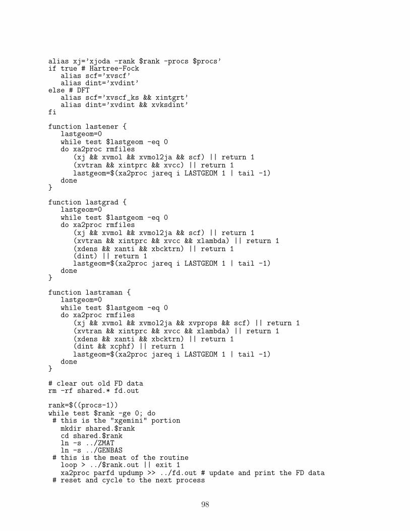
alias xj=’xjoda -rank $rank -procs $procs’if true # Hartree-Fock
alias scf=’xvscf’alias dint=’xvdint’
else # DFTalias scf=’xvscf_ks && xintgrt’alias dint=’xvdint && xvksdint’
fi
function lastener {lastgeom=0while test $lastgeom -eq 0do xa2proc rmfiles
(xj && xvmol && xvmol2ja && scf) || return 1(xvtran && xintprc && xvcc) || return 1lastgeom=$(xa2proc jareq i LASTGEOM 1 | tail -1)
done}
function lastgrad {lastgeom=0while test $lastgeom -eq 0do xa2proc rmfiles
(xj && xvmol && xvmol2ja && scf) || return 1(xvtran && xintprc && xvcc && xlambda) || return 1(xdens && xanti && xbcktrn) || return 1(dint) || return 1lastgeom=$(xa2proc jareq i LASTGEOM 1 | tail -1)
done}
function lastraman {lastgeom=0while test $lastgeom -eq 0do xa2proc rmfiles
(xj && xvmol && xvmol2ja && xvprops && scf) || return 1(xvtran && xintprc && xvcc && xlambda) || return 1(xdens && xanti && xbcktrn) || return 1(dint && xcphf) || return 1lastgeom=$(xa2proc jareq i LASTGEOM 1 | tail -1)
done}
# clear out old FD datarm -rf shared.* fd.out
rank=$((procs-1))while test $rank -ge 0; do# this is the "xgemini" portion
mkdir shared.$rankcd shared.$rankln -s ../ZMATln -s ../GENBAS
# this is the meat of the routineloop > ../$rank.out || exit 1xa2proc parfd updump >> ../fd.out # update and print the FD data
# reset and cycle to the next process
98
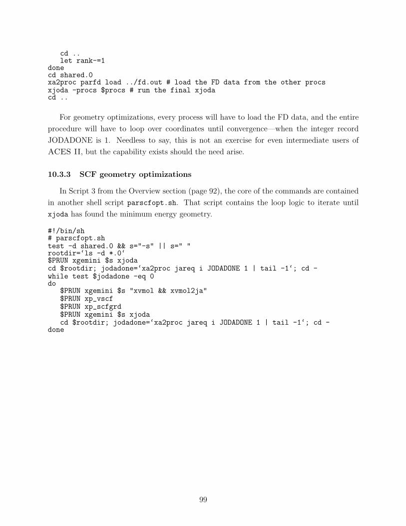
cd ..let rank-=1
donecd shared.0xa2proc parfd load ../fd.out # load the FD data from the other procsxjoda -procs $procs # run the final xjodacd ..
For geometry optimizations, every process will have to load the FD data, and the entire
procedure will have to loop over coordinates until convergence—when the integer record
JODADONE is 1. Needless to say, this is not an exercise for even intermediate users of
ACES II, but the capability exists should the need arise.
10.3.3 SCF geometry optimizations
In Script 3 from the Overview section (page 92), the core of the commands are contained
in another shell script parscfopt.sh. That script contains the loop logic to iterate until
xjoda has found the minimum energy geometry.
#!/bin/sh# parscfopt.shtest -d shared.0 && s="-s" || s=" "rootdir=‘ls -d *.0‘$PRUN xgemini $s xjodacd $rootdir; jodadone=‘xa2proc jareq i JODADONE 1 | tail -1‘; cd -while test $jodadone -eq 0do
$PRUN xgemini $s "xvmol && xvmol2ja"$PRUN xp_vscf$PRUN xp_scfgrd$PRUN xgemini $s xjodacd $rootdir; jodadone=‘xa2proc jareq i JODADONE 1 | tail -1‘; cd -
done
99
11 Troubleshooting
11.1 Common mistakes
The following tips should help users to detect and avoid errors. For large calculations, it is
strongly recommended that users run with trial input files (small basis set, high convergence
tolerances, etc.) before running the actual system.
• The *ACES2 namelist is not terminated properly. If it begins with an open parenthesis,
then it must end with a close parenthesis; otherwise, it must end with a blank line.
Even if the namelist is terminated with a close parenthesis, there must be a blank line
after the namelist and the end-of-file mark.
• The BASIS=SPECIAL option is used but the order of the basis sets does not corre-
spond to the order of atoms in the Z matrix. The code does not check this and will not
crash! For example, one is allowed to put a C basis set on a CL atom. In fact, ghost
atoms would not be possible without this feature.
• All atomic symbols should be in upper case. For example, “Cl” has to be entered as
“CL”. Actually, this is not true anymore, but older versions of the code would simply
give incorrect results. If any user finds case-sensitivity in the coordinate matrix parsing,
[email protected] should be notified with the failing ZMAT.
• Lower case characters have been used instead of upper case. This situation is difficult
to pinpoint. Most of the *ACES2 namelist parsing is case insensitive, along with the
atomic symbols. File directives in the header are still case sensitive as are basis set
names.
• The OCCUPATION keyword takes precedent over CHARGE and MULTIPLICITY.
This can lead to confusion in open-shell SCF calculations. Here are some usage tips:
1. If OCCUPATION has been specified, then the CHARGE and MULTIPLICITY
keywords are ignored. It is, however, good practice to make these consistent with
OCCUPATION
2. If the REFERENCE keyword is absent from an open-shell calculation or is erro-
neously set to RHF, then unpredictable things might happen. ACES II does not
have a default type of open-shell SCF.
3. The occupation specified in the GUESS file takes precedent over all keywords.
Again, it is sensible to make them the same to avoid confusion.
100
4. In older binaries, specifying only the α occupation with OCCUPATION dropped
all β electrons. This is trapped in the current version.
• An input file contains text beyond the 80th column.
• There is no title line, and the first line of the Z matrix has been entered as the title.
• There were files from a previous ACES II calculation in the workspace. In general,
one should clear the workspace of all previous ACES II files prior to copying in the
new files.
11.2 Basic program restrictions
• ZMAT should not change during a running calculation. There might be some hacks that
involve changing convergence tolerances mid-stream, but these are not documented,
supported, or advised.
11.3 Suggestions for reducing resources
• ABCDTYPE=AOBASIS
This saves disk space for CC methods.
• SINGLE STORE=ON
This saves disk space for correlated methods.
• DIRECT,INTEGRALS=GAMESS,FOCK=AO,SYMMETRY=OFF
This save disk space for all calculations, but only applies to SCF and MBPT(2) theories
(without DROPMO).
101
12 References
Of the many methods currently implemented in ACES II, some are well established,
while others are new and descriptions have not yet been published. It is the purpose of
this section to list pertinent literature references which provide more information about
the techniques and their implementations and should be cited when results from ACES II
calculations are published. Some references to basis sets included in the program are also
included.
Guide to Correlated Methods
• R.J. Bartlett and J.F. Stanton, “Applications of Post-Hartree-Fock Methods: A Tuto-
rial”, in Reviews of Computational Chemistry 5, 65-169, edited by K.B. Lipkowitz and
D.B. Boyd (VCH Publishers, New York, 1994).
• R.J. Bartlett, “Coupled-Cluster Theory: An Overview of Recent Developments”, in
Modern Electronic Structure Theory, Part I, edited by D.R. Yarkony (World Scientific
Publishing Co., Singapore, 1995).
12.1 Many-body perturbation theory (MBPT)
Review article
• R.J. Bartlett, Ann. Rev. Phys. Chem. 32, 359 (1981).
a) Closed-shell RHF-MBPT for molecules
• R.J. Bartlett and D.M. Silver, Phys. Rev. A10, 1927 (1974); J. Chem. Phys. 62,
3258 (1975); ibid. 64, 4578 (1976).
• R.J. Bartlett and I. Shavitt, Chem. Phys. Lett. 50, 190 (1977).
b) Open-shell UHF-MBPT for molecules
• R.J. Bartlett and G.D. Purvis III, Int. J. Quantum Chem. 14, 561 (1978).
c) Open-shell ROHF-MBPT for molecules
• W.J. Lauderdale, J.F. Stanton, J. Gauss, J.D. Watts, and R.J. Bartlett, Chem. Phys.
Lett. 187, 21 (1991); J. Chem. Phys. 97, 6606 (1992).
102
12.2 Coupled-cluster (CC) theory
Review article
• R.J. Bartlett, J. Phys. Chem. 93, 1697 (1989).
a) CCD method
• R.J. Bartlett and G.D. Purvis III, Int. J. Quantum Chem. 14, 561 (1978).
b) CCSD method
• G.D. Purvis III and R.J. Bartlett, J. Chem. Phys. 76, 1910 (1982).
c) CCSDT-1 method
• Y.S. Lee, S.A. Kucharski, and R.J. Bartlett, J. Chem. Phys. 81, 5906 (1984).
d) CCSD+T(CCSD) method
• M. Urban, J. Noga, S.J. Cole, and R.J. Bartlett, J. Chem. Phys. 83, 4041 (1985).
e) CCSD(T) method (adds one (HF case) or two (non-HF case) small terms to CCSD+T(CCSD))
• K. Raghavachari, G.W. Trucks, J.A. Pople, and M. Head-Gordon, Chem. Phys. Lett.
157, 479 (1989).
• R.J.Bartlett, J.D.Watts, S.A.Kucharski, and J.Noga, Chem. Phys. Lett. 165, 513
(1990).
• J. Gauss, W.J. Lauderdale, J.F. Stanton, J.D. Watts, and R.J. Bartlett, Chem. Phys.
Lett. 182, 207 (1991).
• J.D. Watts, J. Gauss, and R.J. Bartlett, J. Chem. Phys. 98, 8718 (1993).
f) CCSDT-2 and CCSDT-3 methods
• J.Noga, R.J.Bartlett, and M.Urban, Chem. Phys. Lett. 134, 146 (1987).
g) CCSDT methods
• J. Noga and R.J. Bartlett, J. Chem. Phys. 86, 7041 (1987).
• G.E. Scuseria and H.F. Schaefer, Chem. Phys. Lett. 152, 382 (1988).
103
• J.D. Watts and R.J. Bartlett, J. Chem. Phys. 93, 6104 (1990).
• J.D. Watts and R.J. Bartlett, Int. J. Quant. Chem. Symp. 27, 51 (1993).
h) ROHF and QRHF CC methods
• M.Rittby and R.J.Bartlett, J. Phys. Chem. 92, 3033 (1988).
i) Brueckner CC methods
• R.A. Chiles and C.E. Dykstra, J. Chem. Phys. 74, 4544 (1981).
• J.F.Stanton, J.Gauss, and R.J.Bartlett, J. Chem. Phys. 97, 5554 (1992).
j) QCISD and QCISD(T) methods
• J.A. Pople, M. Head-Gordon, and K. Raghavachari J. Chem. Phys. 87, 5968 (1987).
k) UCC methods
• J.D. Watts, G.W. Trucks, and R.J. Bartlett, Chem. Phys. Lett. 157, 359 (1989).
l) CCSD+TQ*(CCSD), CCSD(TQ), and QCISD(TQ) methods
• R.J. Bartlett, J.D. Watts, S.A. Kucharski, and J. Noga, Chem. Phys. Lett. 165, 513
(1990).
• K. Raghavachari, J.A. Pople, E.S. Replogle, and M. Head-Gordon, J. Phys. Chem.
94, 5579 (1990).
m) Two-determinant CCSD method
• A. Balkova and R.J. Bartlett, Chem. Phys. Lett. 193, 364 (1992).
12.3 Analytical gradients for MBPT/CC methods
Review article
• R.J.Bartlett, J.F.Stanton, and J.D.Watts, in Advances in Molecular Vibrations and
Collision Dynamics, Vol. 1, ed. J.Bowman, JAI Press, p. 139 (1991).
• J. Gauss and D. Cremer, Adv. Quant. Chem. 23, 205 (1992).
a) General MBPT/CC gradient theory
104
• E.A.Salter, G.W.Trucks, and R.J.Bartlett, J. Chem. Phys. 90, 1752 (1989).
b) Implementation for closed- and open-shell CCSD
• J.Gauss, J.F.Stanton, and R.J.Bartlett, J. Chem. Phys. 95, 2623 (1991).
c) QRHF-CCSD gradients
• J.Gauss, J.F.Stanton, and R.J.Bartlett, J. Chem. Phys. 95, 2639 (1991).
d) ROHF-CCSD gradients
• J.Gauss, W.J.Lauderdale, J.F.Stanton, J.D.Watts, and R.J.Bartlett, Chem. Phys.
Lett. 182, 207 (1991).
e) QCISD gradients
• J. Gauss and D. Cremer, Chem. Phys. Lett. 150, 280 (1988).
• J.Gauss, J.F.Stanton, and R.J.Bartlett, J. Chem. Phys. 95, 2623 (1991).
f) MBPT(4) gradients for closed- and open-shells
• J. Gauss and D. Cremer, Chem. Phys. Lett. 138, 131 (1987); 153, 303 (1988).
• G.W.Trucks, J.D.Watts, E.A.Salter, and R.J.Bartlett, Chem. Phys. Lett. 153, 490
(1988).
• J.D.Watts, G.W.Trucks, and R.J.Bartlett, Chem. Phys. Lett. 164, 502 (1989).
• J.D.Watts, J. Gauss, and R.J.Bartlett, Chem. Phys. Lett. 200, 1 (1992).
g) CCSD+T(CCSD), CCSD(T) gradients for closed- and open-shells
• J.D.Watts, J. Gauss, and R.J.Bartlett, Chem. Phys. Lett. 200, 1 (1992).
• J.D. Watts, J. Gauss, and R.J. Bartlett, J. Chem. Phys. 98, 8718 (1993).
h) QCISD(T) gradients
• J. Gauss and D. Cremer, Chem. Phys. Lett. 163, 549 (1990).
• J.D.Watts, J. Gauss, and R.J.Bartlett, Chem. Phys. Lett. 200, 1 (1992).
i) UCC(4) gradients for closed- and open-shells
• J.D.Watts, G.W.Trucks, and R.J.Bartlett, Chem. Phys. Lett. 157, 359 (1989).
• J.D.Watts, G.W.Trucks, and R.J.Bartlett, Chem. Phys. Lett. 164, 502 (1989).
j) Two-determinant CCSD (TD-CCSD) analytical gradients for open-shell singlet states
• P.G. Szalay and R.J. Bartlett, J. Chem. Phys. 101, 4936 (1994).
105
12.4 Analytical second derivatives for MBPT/CC methods
a) MBPT(2) second derivatives for closed shells
• N.C. Handy, R.D. Amos, J.F. Gaw, J.E. Rice, E.D. Simandiras, T.J. Lee, R.J. Harrison,
W.D. Laidig, G.B. Fitzgerald and R.J. Bartlett, in Geometrical Derivatives of Energy
Surfaces and Molecular Properties, edited by P. Jørgensen and J. Simons (Reidel,
Dordrecht, 1986).
• N.C. Handy, R.D. Amos, J.F. Gaw, J.E. Rice, E.D. Simandiras, Chem. Phys. Letters
120, 151 (1985).
• R.J. Harrison, G.B. Fitzgerald, W.D. Laidig, R.J. Bartlett, Chem. Phys. Lett. 124,
291 (1986).
b) MBPT(2) second derivatives for open shells (UHF and ROHF)
• J.F. Stanton, J. Gauss, and R.J. Bartlett, Chem. Phys. Lett. 195, 194 (1992).
• J. Gauss, J.F. Stanton, and R.J. Bartlett, J. Chem. Phys. 97, 7825 (1992).
12.5 NMR chemical shift calculations
a) GIAO-SCF NMR chemical shift calculations
• R. Ditchfield, Mol. Phys. 27, 789 (1974).
• K. Wolinski, J.F. Hinton, and P. Pulay, J. Am. Chem. Soc. 112, 8251 (1990).
• M. Haser, R. Ahlrichs, H.P. Baron, P. Weis, and H. Horn, Theoret. Chim. Acta, 83,
455 (1992).
b) GIAO-MBPT(2) NMR chemical shift calculations
• J. Gauss, Chem. Phys. Lett. 191, 614 (1992); J. Chem. Phys. 99, 3629 (1993).
12.6 Methods for calculating excitation energies
a) Tamm-Dancoff (CI singles) approximation
b) Random-Phase approximation (RPA)
c) Equation-of-Motion Coupled Cluster (EOM-CC) methods
• J.F. Stanton and R.J. Bartlett, J. Chem. Phys. 98, 7029 (1993)
106
12.7 Methods for calculating electron attachment energies
The electron affinity equation-of-motion coupled-cluster method :
• M. Nooijen and R.J. Bartlett, J. Chem. Phys. 102, 3629 (1995).
12.8 Time-dependent Hartree-Fock methods
• H. Sekino and R.J. Bartlett, J. Chem. Phys. 85, 976 (1986).
• H. Sekino and R.J. Bartlett, Int. J. Quantum Chem. 43, 119 (1992).
12.9 HF-DFT method
• P. M. W. Gill, B. G. Johnson, and J. A. Pople, Int. J. Quantum Chem. Symp. 26,
319 (1992).
• G. E. Scuseria, J. Chem. Phys. 97, 7528 (1992).
• N. Oliphant and R. J. Bartlett, J. Chem. Phys. 100, 6550 (1994).
12.10 Basis sets
STO-3G
• W.J.Hehre, R.F.Stewart, and J.A.Pople, J. Chem. Phys. 51, 2657 (1969); first-row
elements.
• W.J.Hehre, R.Ditchfield, R.F.Stewart, and J.A.Pople, J. Chem. Phys. 52, 2769 (1970);
second-row elements and improved scale factors for Li and Be.
• W.J.Pietro, B.A.Levi, W.J.Hehre, and R.F.Stewart, Inorg. Chem. 19, 2225 (1980);
third-row elements.
• W.J.Pietro, E.S.Blurock, R.F.Hout,Jr, W.J.Hehre, D.J.DeFrees, and R.F.Stewart, In-
org. Chem. 20, 3650 (1981); fourth-row elements.
• W.J.Pietro and W.J.Hehre, J. Comput. Chem. 4, 241 (1983); first- and second-row
transition metal elements.
3-21G
• J.S.Binkley, J.A.Pople, and W.J.Hehre, J. Am. Chem. Soc. 102, 939 (1980); first-row
elements.
107
• M.S.Gordon, J.S.Binkley, J.A.Pople, W.J.Pietro, and W.J.Hehre, J. Am. Chem. Soc.
104, 2797 (1982); second-row elements.
4-31G
• R.Ditchfield, W.J.Hehre, and J.A.Pople, J. Chem. Phys. 54, 724 (1971); H,C,O,N,
and F.
• W.J.Hehre and J.A.Pople, J. Chem. Phys. 56, 4233 (1972); B.
• W.J.Hehre and W.A.Lathan, J. Chem. Phys. 56, 5255 (1972); P,S, and Cl.
6-31G
• W.J.Hehre, R.Ditchfield, and J.A.Pople, J. Chem. Phys. 56, 2257 (1972); C,N,O, and
F.
• J.D.Dill and J.A.Pople, J. Chem. Phys. 62, 2921 (1975); Li,Be,B.
• M.M.Francl, W.J.Pietro, W.J.Hehre, J.S.Binkley, M.S.Gordon, D.J.DeFrees, and J.A.Pople,
J. Chem. Phys. 77, 3654 (1982); second-row elements.
6-31G* (and 6-31G**)
• P.C.Hariharan and J.A.Pople, Theor. Chim. Acta 28, 213 (1973); first-row elements.
• M.M.Francl, W.J.Pietro, W.J.Hehre, J.S.Binkley, M.S.Gordon, D.J.DeFrees, and J.A.Pople,
J. Chem. Phys. 77, 3654 (1982); second-row elements.
6-311G**
• R.Krishnan, J.S.Binkley, R.Seeger, and J.A.Pople, J. Chem. Phys. 72, 650 (1980);
first-row elements.
Dunning basis sets
• T.H.Dunning, Jr, J. Chem. Phys. 53, 2823 (1970); double-zeta and triple-zeta valence
contractions of 9s5p primitive set for H,B-F, including 4s2p and 4s3p.
• T.H.Dunning, Jr, J. Chem. Phys. 55, 716 (1971); triple-zeta valence and more flex-
ible contractions of 10s6p primitive set for H,B-F, including 5s3p and 5s4p. Also 4s
contraction for Li, 5s contraction for Be.
108
• T.H.Dunning, Jr and P.J.Hay, in Methods of Electronic Structure Theory, edited by
H.F.Schaefer III, Plenum, New York, 1977; 6s4p contractions of 11s7p for Al-Cl (Cl
basis contains typographical errors, see Craven et al, Chem. Phys. Lett. 116, 119
(1985)); VDZP basis set for first-row elements; diffuse and Rydberg functions; recom-
mended polarization exponents from SCF calculations.
• T.H.Dunning, Jr, J. Chem. Phys. 90, 1007 (1989) (PVDZ-PVQZ); R.A. Kendall, T.H.
Dunning, Jr, and R.J. Harrison, J. Chem. Phys. 96, 6796 (1992) (diffuse functions for
PVDZ to PVQZ); D.E. Woon and T.H. Dunning, Jr, J. Chem. Phys. 98, 1358 (1993)
(PV5Z and diffuse functions for PV5Z); methodology of the “correlation consistent”
sets, but does not include the actual sets : these must be obtained directly from
Dunning via FTP.
Atomic natural orbital basis sets of Roos and coworkers (WMR)
• P.O. Widmark, P.A. Malmqvist, and B.O. Roos, Theor. Chim. Acta 77, 291 (1990).
• P.O. Widmark, B.J. Persson, and B.O. Roos, Theor. Chim. Acta 79, 419 (1991).
Polarized basis sets of Sadlej and coworkers
• A.J. Sadlej, Collec. Czech. Chem. Commun. 53, 1995 (1988).
• A.J. Sadlej and M. Urban, J. Mol. Struct. (THEOCHEM) 234, 147 (1991).
• A.J. Sadlej, Theor. Chim. Acta 79, 123 (1991).
• A.J. Sadlej, Theor. Chim. Acta 81, 45 (1992).
• A.J. Sadlej, Theor. Chim. Acta 81, 339 (1992).
Basis sets optimized by Ahlrichs and coworkers
• A. Schafer, H. Horn, and R. Ahlrichs J. Chem. Phys. 97, 2571 (1992). These basis
sets have been optimized for atoms at the SCF level using analytic gradient techniques
and have been supplemented with a suitable choice of polarization functions. Input in
the ACES II program is in this case always via BASIS=SPECIAL. The actual basis
sets can be obtained via FTP from the authors.
Some other extended basis sets for second-row atoms (sp parts)
• A.D.McLean and G.S.Chandler, J. Chem. Phys. 72, 5639 (1980); up to 6s5p sets for
second-row atoms contracted from up to 12s9p primitive sets.
109
Polarization exponents from correlated calculations
• L.T.Redmon, G.D.Purvis III, and R.J.Bartlett, J. Am. Chem. Soc. 101, 2856 (1979);
recommended polarization exponents for use with DZ basis sets for H,B,C,N, and O.
12.11 Integral packages
The direct integrals are obtained by Rys quadrature (1) using an implementation ex-
tended to spdfg and L shells taken from GAMESS (2).
(1) J. Rys, M. Dupuis, H.F. King. J. Comput. Chem. 4 154-157 (1983).
(2) M.W. Schmidt, K.K. Baldridge, J.A. Boatz, S.T. Elbert, M.S. Gordon, J.J. Jensen,
S. Koseki, N. Matsunaga, K.A. Nguyen, S. Su, T.L. Windus, M. Dupuis, J.A. Mont-
gomery. J. Comput. Chem. 14 1347-1363 (1993).
110
A Other Keywords
A.1 Experimental, obsolete, and unused
The following keywords in the *ACES2 namelist are listed for completeness, but they
correspond to untested and/or experimental code.
SOLVENT = (integer) 0
Sets the dielectric constant used to determine the orbitals. A cavity size may be
specified as well by creating a file named “radius”, which is read by the SCF code.
This contains the cavity radius in A. If the file is not present, the program uses a value
calculated from 0.5 A plus half of the longest internuclear distance.
TURBOMOLE = (switch) OFF
POLYRATE = (switch) OFF
CCR12 = (switch) OFF
KUCHARSKI = (switch) OFF
KS POT Obsoleted by the *VSCF namelist.
FUNCTIONAL Obsoleted by the *INTGRT namelist.
EOMXFIELD
EOMYFIELD
EOMZFIELD
RDO
FILE STRIPE
RESET FLAGS
PSI
INSERTF
GLOBAL MEM
111
A.2 Kohn-Sham DFT namelists
A.2.1 *VSCF
KS = (switch) ON
Controls the type of SCF. KS=ON performs a Kohn-Sham DFT calculation with nu-
merical integration, and KS=OFF performs the standard analytical Hartree-Fock SCF
with the KS SCF program xvscf ks. The *ACES2 keyword SCF TYPE must be set
to KS in addition to this switch, which defaults to ON.
A.2.2 *INTGRT
POTRADPTS = (integer) 50
RADTYP = (handle) Handy
Handy
Gauss-Legendre
PARTPOLY = (handle) bsrad
equal
bsrad
dynamic
RADSCAL = (handle) Slater
none
Slater
PARTTYP = (handle) fuzzy
rigid
fuzzy
FUZZYITER = (integer) 4
RADLIMIT = (real) 3.0
112
NUMACC = (switch) ON
EXACT EX = (switch) OFF
TDKS = (switch) OFF
ENEGRID = (integer) 4
POTGRID = (integer) 4
ENETYPE = (handle) lebedev
POTTYPE = (handle) lebedev
FUNC = (string) none
This keyword can accept multiple types of strings. The regular expression is
exch(,coeff)?(,corr(,coeff)?)?
This means one (exchange) or two (exchange and correlation) functionals can be used
to evaluate the total SCF energy, and each can have an optional coefficient (default
is 1.0). To use B3LYP, the format must be “func=b3lyp” with no coefficients or
additional correlation functionals.
The following exchange (and hybrid) functionals are available:
lda LDA (Slater, Xalpha) (exchange)becke Becke (exchange)hf Exact Nonlocal Exchange (exchange)pbe ex Perdew-Burke-Ernzerhof (exchange)pw91 ex Perdew-Wang 91 (exchange)b3lyp Becke III LYP (hybrid)
The following correlation functionals are available:
vwn Vosko-Wilk-Nusairlyp Lee-Yang-Parrpbe cor Perdew-Burke-Ernzerhofpw91 cor Perdew-Wang 91wl Wilson-Levywi Wilson-Ivanov
KSPOT = (string) hf
The KSPOT value string takes the same format as FUNC. The available exchange
potentials are: lda, becke, and hf. The available correlation potentials are: vwn and
lyp.
CUTOFF = (tol) 12
113

A.3 mrcc namelists
A.3.1 *mrcc gen, *true mrcc, *cse
A.3.2 *EE EOM, *EE TDA, *EE STEOM
A.3.3 *IP EOM, *IP CI, *DIP EOM, *DIP TDA, *DIP STEOM
A.3.4 *EA EOM, *EA CI, *DEA EOM, *DEA TDA, *DEA STEOM
A.3.5 *ACT EA EOM
114
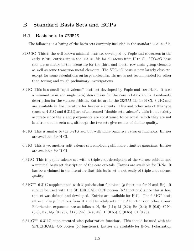
B Standard Basis Sets and ECPs
B.1 Basis sets in GENBAS
The following is a listing of the basis sets currently included in the standard GENBAS file.
STO-3G This is the well known minimal basis set developed by Pople and coworkers in the
early 1970s. entries are in the GENBAS file for all atoms from H to Cl. STO-3G basis
sets are available in the literature for the third and fourth row main group elements
as well as some transition metal elements. The STO-3G basis is now largely obsolete,
except for some calculations on large molecules. Its use is not recommended for other
than testing and rough preliminary investigations.
3-21G This is a small “split valence” basis set developed by Pople and coworkers. It uses
a minimal basis (or single zeta) description for the core orbitals and a double-zeta
description for the valence orbitals. Entries are in the GENBAS file for H-Cl. 3-21G sets
are available in the literature for heavier elements. This and other sets of this type
(such as 4-31G and 6-31G) are often termed “double zeta valence”. This is not strictly
accurate since the s and p exponents are constrained to be equal, which they are not
in a true double zeta set, although the two sets give results of similar quality.
4-31G This is similar to the 3-21G set, but with more primitive gaussian functions. Entries
are available for H-Cl.
6-31G This is yet another split valence set, employing still more primitive gaussians. Entries
are available for H-Cl.
6-311G This is a split valence set with a triple-zeta description of the valence orbitals and
a minimal basis set description of the core orbitals. Entries are available for H-Ne. It
has been claimed in the literature that this basis set is not really of triple-zeta valence
quality.
6-31G** 6-31G supplemented with d polarization functions (p functions for H and He). It
should be used with the SPHERICAL=OFF option (6d functions) since this is how
the set was defined and developed. Entries are available for H-Cl. The 6-31G* basis
set excludes p functions from H and He, while retaining d functions on other atoms.
Polarization exponents are as follows: H, He (1.1); Li (0.2); Be (0.4); B (0.6); C-Ne
(0.8); Na, Mg (0.175); Al (0.325); Si (0.45); P (0.55); S (0.65); Cl (0.75).
6-311G** 6-311G supplemented with polarization functions. This should be used with the
SPHERICAL=ON option (5d functions). Entries are available for H-Ne. Polarization
115
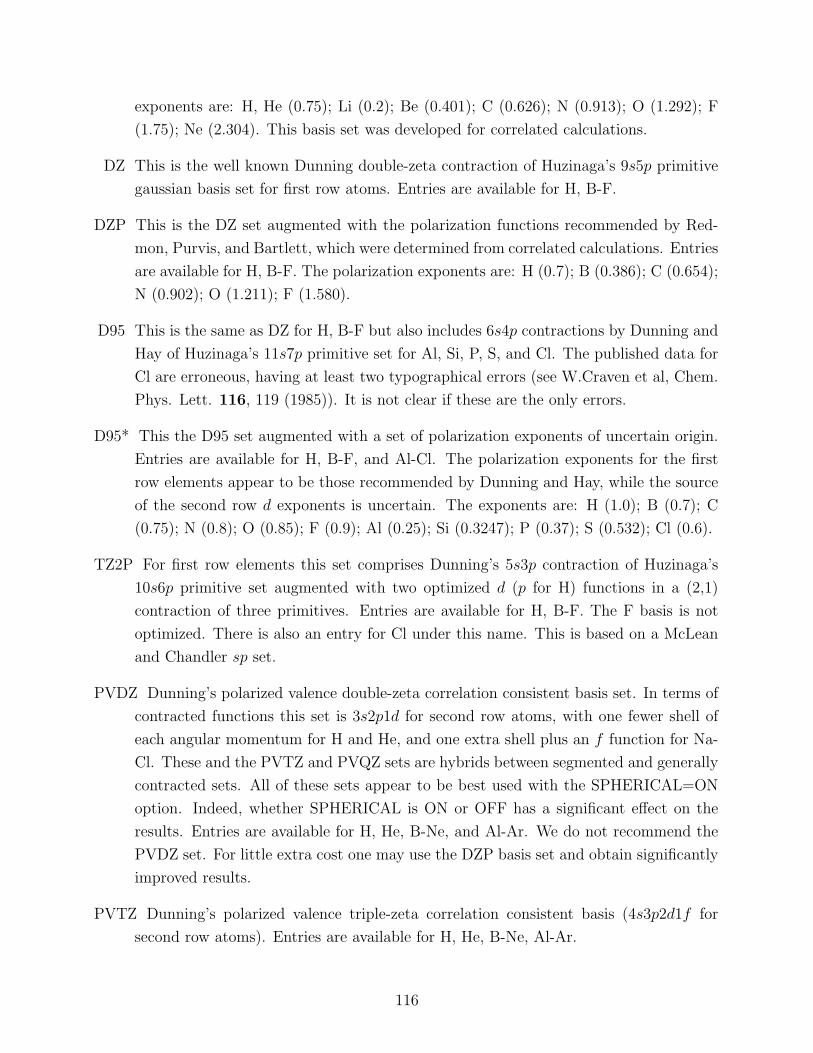
exponents are: H, He (0.75); Li (0.2); Be (0.401); C (0.626); N (0.913); O (1.292); F
(1.75); Ne (2.304). This basis set was developed for correlated calculations.
DZ This is the well known Dunning double-zeta contraction of Huzinaga’s 9s5p primitive
gaussian basis set for first row atoms. Entries are available for H, B-F.
DZP This is the DZ set augmented with the polarization functions recommended by Red-
mon, Purvis, and Bartlett, which were determined from correlated calculations. Entries
are available for H, B-F. The polarization exponents are: H (0.7); B (0.386); C (0.654);
N (0.902); O (1.211); F (1.580).
D95 This is the same as DZ for H, B-F but also includes 6s4p contractions by Dunning and
Hay of Huzinaga’s 11s7p primitive set for Al, Si, P, S, and Cl. The published data for
Cl are erroneous, having at least two typographical errors (see W.Craven et al, Chem.
Phys. Lett. 116, 119 (1985)). It is not clear if these are the only errors.
D95* This the D95 set augmented with a set of polarization exponents of uncertain origin.
Entries are available for H, B-F, and Al-Cl. The polarization exponents for the first
row elements appear to be those recommended by Dunning and Hay, while the source
of the second row d exponents is uncertain. The exponents are: H (1.0); B (0.7); C
(0.75); N (0.8); O (0.85); F (0.9); Al (0.25); Si (0.3247); P (0.37); S (0.532); Cl (0.6).
TZ2P For first row elements this set comprises Dunning’s 5s3p contraction of Huzinaga’s
10s6p primitive set augmented with two optimized d (p for H) functions in a (2,1)
contraction of three primitives. Entries are available for H, B-F. The F basis is not
optimized. There is also an entry for Cl under this name. This is based on a McLean
and Chandler sp set.
PVDZ Dunning’s polarized valence double-zeta correlation consistent basis set. In terms of
contracted functions this set is 3s2p1d for second row atoms, with one fewer shell of
each angular momentum for H and He, and one extra shell plus an f function for Na-
Cl. These and the PVTZ and PVQZ sets are hybrids between segmented and generally
contracted sets. All of these sets appear to be best used with the SPHERICAL=ON
option. Indeed, whether SPHERICAL is ON or OFF has a significant effect on the
results. Entries are available for H, He, B-Ne, and Al-Ar. We do not recommend the
PVDZ set. For little extra cost one may use the DZP basis set and obtain significantly
improved results.
PVTZ Dunning’s polarized valence triple-zeta correlation consistent basis (4s3p2d1f for
second row atoms). Entries are available for H, He, B-Ne, Al-Ar.
116
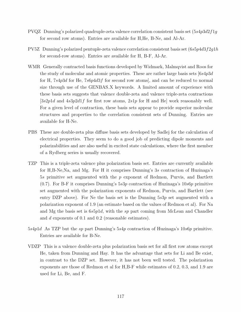
PVQZ Dunning’s polarized quadruple-zeta valence correlation consistent basis set (5s4p3d2f1g
for second row atoms). Entries are available for H,He, B-Ne, and Al-Ar.
PV5Z Dunning’s polarized pentuple-zeta valence correlation consistent basis set (6s5p4d3f2g1h
for second-row atoms). Entries are available for H, B-F, Al-Ar.
WMR Generally contracted basis functions developed by Widmark, Malmqvist and Roos for
the study of molecular and atomic properties. These are rather large basis sets [6s4p3d
for H, 7s4p3d for He, 7s6p4d3f for second row atoms], and can be reduced to normal
size through use of the GENBAS X keywords. A limited amount of experience with
these basis sets suggests that valence double-zeta and valence triple-zeta contractions
[3s2p1d and 4s3p2d1f for first row atoms, 2s1p for H and He] work reasonably well.
For a given level of contraction, these basis sets appear to provide superior molecular
structures and properties to the correlation consistent sets of Dunning. Entries are
available for H-Ne.
PBS These are double-zeta plus diffuse basis sets developed by Sadlej for the calculation of
electrical properties. They seem to do a good job of predicting dipole moments and
polarizabilities and are also useful in excited state calculations, where the first member
of a Rydberg series is usually recovered.
TZP This is a triple-zeta valence plus polarization basis set. Entries are currently available
for H,B-Ne,Na, and Mg. For H it comprises Dunning’s 3s contraction of Huzinaga’s
5s primitive set augmented with the p exponent of Redmon, Purvis, and Bartlett
(0.7). For B-F it comprises Dunning’s 5s3p contraction of Huzinaga’s 10s6p primitive
set augmented with the polarization exponents of Redmon, Purvis, and Bartlett (see
entry DZP above). For Ne the basis set is the Dunning 5s3p set augmented with a
polarization exponent of 1.9 (an estimate based on the values of Redmon et al). For Na
and Mg the basis set is 6s5p1d, with the sp part coming from McLean and Chandler
and d exponents of 0.1 and 0.2 (reasonable estimates).
5s4p1d As TZP but the sp part Dunning’s 5s4p contraction of Huzinaga’s 10s6p primitive.
Entries are available for B-Ne.
VDZP This is a valence double-zeta plus polarization basis set for all first row atoms except
He, taken from Dunning and Hay. It has the advantage that sets for Li and Be exist,
in contrast to the DZP set. However, it has not been well tested. The polarization
exponents are those of Redmon et al for H,B-F while estimates of 0.2, 0.3, and 1.9 are
used for Li, Be, and F.
117
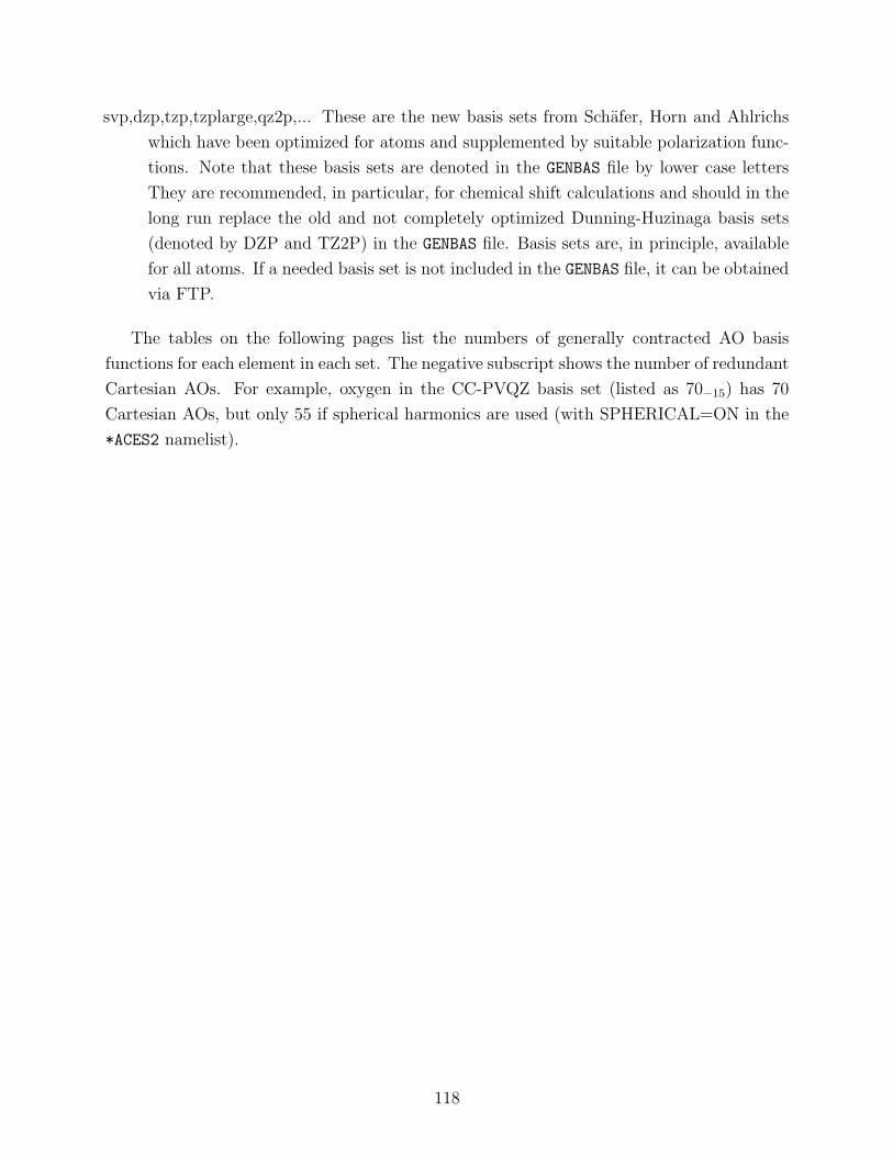
svp,dzp,tzp,tzplarge,qz2p,... These are the new basis sets from Schafer, Horn and Ahlrichs
which have been optimized for atoms and supplemented by suitable polarization func-
tions. Note that these basis sets are denoted in the GENBAS file by lower case letters
They are recommended, in particular, for chemical shift calculations and should in the
long run replace the old and not completely optimized Dunning-Huzinaga basis sets
(denoted by DZP and TZ2P) in the GENBAS file. Basis sets are, in principle, available
for all atoms. If a needed basis set is not included in the GENBAS file, it can be obtained
via FTP.
The tables on the following pages list the numbers of generally contracted AO basis
functions for each element in each set. The negative subscript shows the number of redundant
Cartesian AOs. For example, oxygen in the CC-PVQZ basis set (listed as 70−15) has 70
Cartesian AOs, but only 55 if spherical harmonics are used (with SPHERICAL=ON in the
*ACES2 namelist).
118
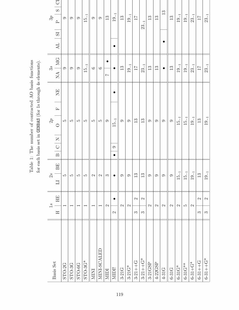
Tab
le1:
The
num
ber
ofco
ntr
acte
dA
Obas
isfu
nct
ions
for
each
bas
isse
tin
GENBAS
(for
1sth
rough
4sel
emen
ts).
Bas
isSet
1s2s
2p3s
3p4s
HH
ELI
BE
BC
NO
FN
EN
AM
GA
LSI
PS
CL
AR
KC
A
ST
O-2
G1
55
99
13
ST
O-3
G1
55
99
13
ST
O-6
G1
55
99
13
ST
O-3
G*
15
515
−1
15−
1•
MIN
I1
25
69
10
MIN
I-SC
ALE
D1
25
69
10
MID
I2
39
7•
1311
•M
IDI!
2•
••
915
−1
••
•19
−1
••
3-21
G2
99
1313
17
3-21
G*
29
919
−1
19−
1•
3-21
++
G3
213
1317
17•
3-21
++
G*
32
1313
23−
123
−1
17•
3-21
GSP
29
913
13•
4-22
GSP
29
913
13•
4-31
G2
99
••
13•
•6-
31G
29
913
1317
6-31
G*
215
−1
15−
119
−1
19−
123
−1
6-31
G**
515
−1
15−
119
−1
19−
123
−1
6-31
+G
*2
19−
119
−1
23−
123
−1
•6-
31+
+G
32
1313
1717
21
6-31
++
G*
32
19−
119
−1
23−
123
−1
•
119
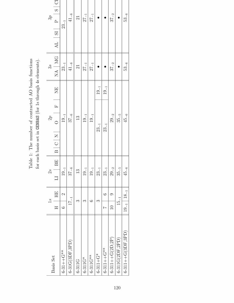
Tab
le1:
The
num
ber
ofco
ntr
acte
dA
Obas
isfu
nct
ions
for
each
bas
isse
tin
GENBAS
(for
1sth
rough
4sel
emen
ts).
Bas
isSet
1s2s
2p3s
3p4s
HH
ELI
BE
BC
NO
FN
EN
AM
GA
LSI
PS
CL
AR
KC
A
6-31
++
G**
62
19−
119
−1
23−
123
−1
17•
6-31
G(3
DF,3
PD
)17
−1
37−
637
−6
41−
641
−6
•6-
311G
313
1321
2135
−1
6-31
1G*
319
−1
19−
127
−1
27−
141
−2
6-31
1G**
619
−1
19−
127
−1
27−
141
−2
6-31
1+G
*3
23−
123
−1
19−
1•
••
6-31
1++
G**
76
23−
123
−1
19−
1•
••
6-31
1++
G(2
D,2
P)
109
29−
229
−2
37−
237
−2
51−
3
6-31
1G(2
DF,2
PD
)15
−1
35−
535
−5
••
57−
6
6-31
1++
G(3
DF,3
PD
)19
−1
18−
145
−6
45−
653
−6
53−
6•
120
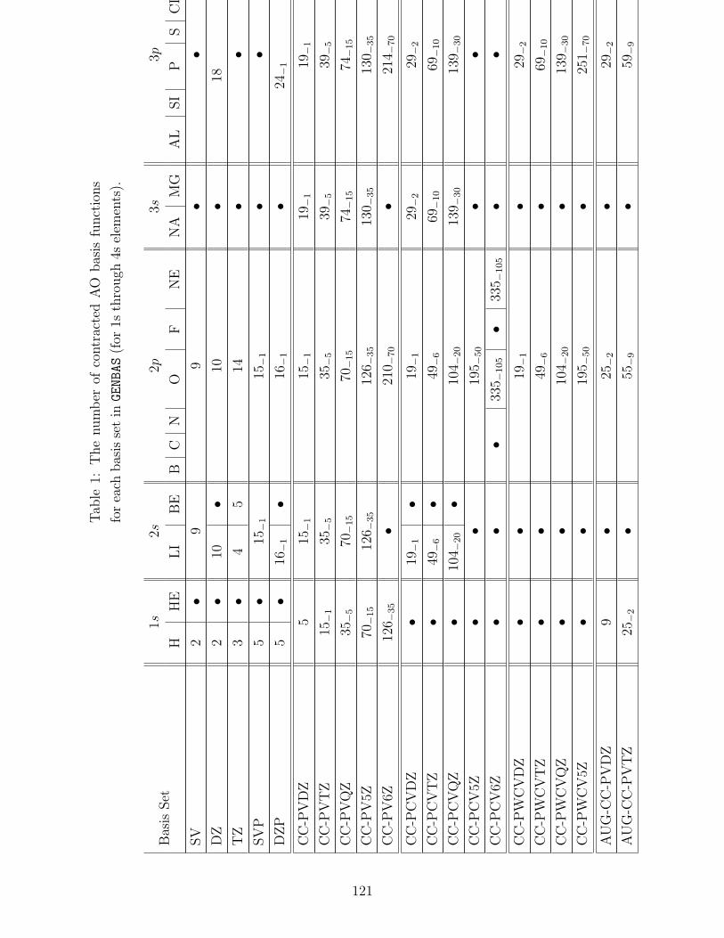
Tab
le1:
The
num
ber
ofco
ntr
acte
dA
Obas
isfu
nct
ions
for
each
bas
isse
tin
GENBAS
(for
1sth
rough
4sel
emen
ts).
Bas
isSet
1s2s
2p3s
3p4s
HH
ELI
BE
BC
NO
FN
EN
AM
GA
LSI
PS
CL
AR
KC
A
SV
2•
99
••
•D
Z2
•10
•10
•18
••
TZ
3•
45
14•
••
SV
P5
•15
−1
15−
1•
••
DZP
5•
16−
1•
16−
1•
24−
1•
•C
C-P
VD
Z5
15−
115
−1
19−
119
−1
•29
−2
CC
-PV
TZ
15−
135
−5
35−
539
−5
39−
5•
49−
6
CC
-PV
QZ
35−
570
−15
70−
15
74−
15
74−
15
•84
−16
CC
-PV
5Z70
−15
126 −
35
126 −
35
130 −
35
130 −
35
•14
0 −36
CC
-PV
6Z12
6 −35
•21
0 −70
•21
4 −70
•C
C-P
CV
DZ
•19
−1
•19
−1
29−
229
−2
•C
C-P
CV
TZ
•49
−6
•49
−6
69−
10
69−
10
•C
C-P
CV
QZ
•10
4 −20
•10
4 −20
139 −
30
139 −
30
•C
C-P
CV
5Z•
•19
5 −50
••
•C
C-P
CV
6Z•
••
335 −
105
•33
5 −105
••
•C
C-P
WC
VD
Z•
•19
−1
•29
−2
•C
C-P
WC
VT
Z•
•49
−6
•69
−10
•C
C-P
WC
VQ
Z•
•10
4 −20
•13
9 −30
•C
C-P
WC
V5Z
••
195 −
50
•25
1 −70
•A
UG
-CC
-PV
DZ
9•
25−
2•
29−
2•
AU
G-C
C-P
VT
Z25
−2
•55
−9
•59
−9
•
121
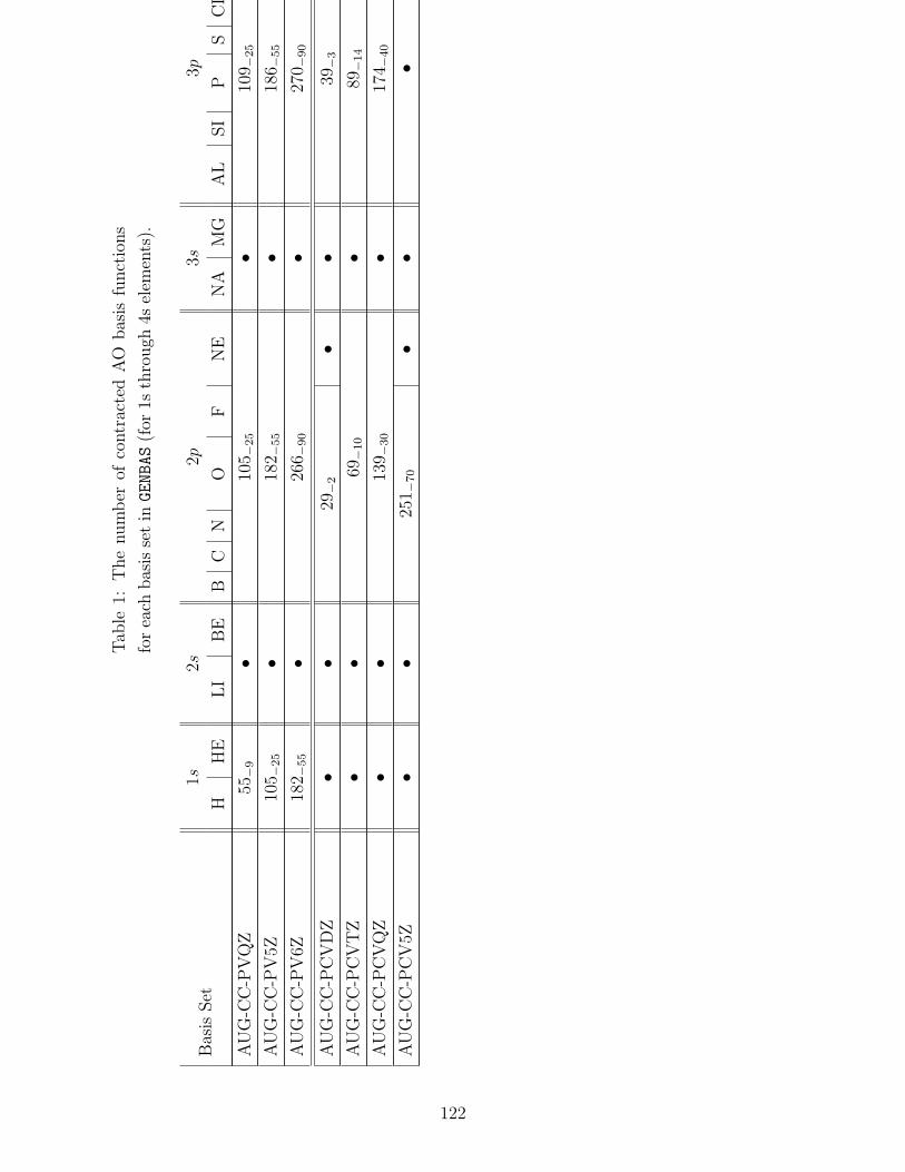
Tab
le1:
The
num
ber
ofco
ntr
acte
dA
Obas
isfu
nct
ions
for
each
bas
isse
tin
GENBAS
(for
1sth
rough
4sel
emen
ts).
Bas
isSet
1s2s
2p3s
3p4s
HH
ELI
BE
BC
NO
FN
EN
AM
GA
LSI
PS
CL
AR
KC
A
AU
G-C
C-P
VQ
Z55
−9
•10
5 −25
•10
9 −25
•A
UG
-CC
-PV
5Z10
5 −25
•18
2 −55
•18
6 −55
•A
UG
-CC
-PV
6Z18
2 −55
•26
6 −90
•27
0 −90
•A
UG
-CC
-PC
VD
Z•
•29
−2
••
39−
3•
AU
G-C
C-P
CV
TZ
••
69−
10
•89
−14
•A
UG
-CC
-PC
VQ
Z•
•13
9 −30
•17
4 −40
•A
UG
-CC
-PC
V5Z
••
251 −
70
••
••
122
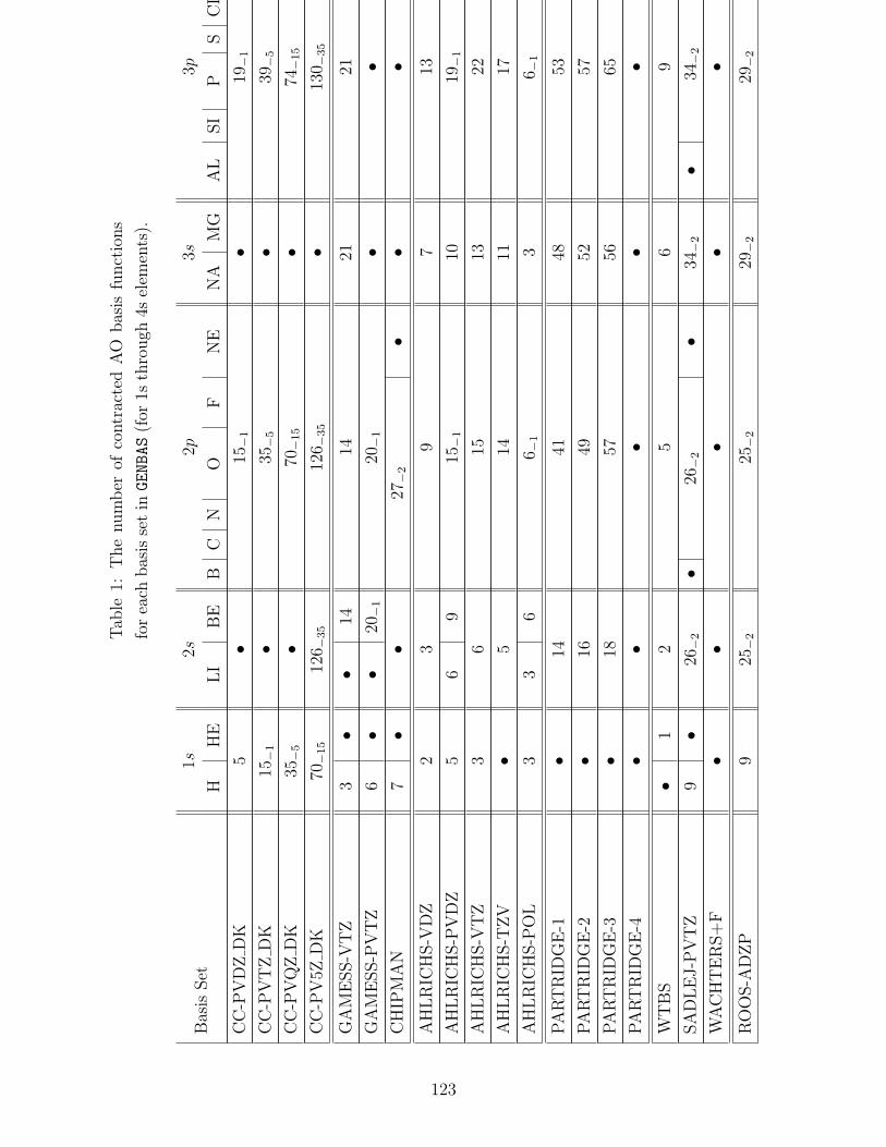
Tab
le1:
The
num
ber
ofco
ntr
acte
dA
Obas
isfu
nct
ions
for
each
bas
isse
tin
GENBAS
(for
1sth
rough
4sel
emen
ts).
Bas
isSet
1s2s
2p3s
3p4s
HH
ELI
BE
BC
NO
FN
EN
AM
GA
LSI
PS
CL
AR
KC
A
CC
-PV
DZ
DK
5•
15−
1•
19−
1•
CC
-PV
TZ
DK
15−
1•
35−
5•
39−
5•
CC
-PV
QZ
DK
35−
5•
70−
15
•74
−15
•C
C-P
V5Z
DK
70−
15
126 −
35
126 −
35
•13
0 −35
•G
AM
ESS-V
TZ
3•
•14
1421
21•
GA
ME
SS-P
VT
Z6
••
20−
120
−1
••
•C
HIP
MA
N7
••
27−
2•
••
•A
HLR
ICH
S-V
DZ
23
97
1311
AH
LR
ICH
S-P
VD
Z5
69
15−
110
19−
114
AH
LR
ICH
S-V
TZ
36
1513
2223
AH
LR
ICH
S-T
ZV
•5
1411
1715
AH
LR
ICH
S-P
OL
33
66 −
13
6 −1
3
PA
RT
RID
GE
-1•
1441
4853
56
PA
RT
RID
GE
-2•
1649
5257
64
PA
RT
RID
GE
-3•
1857
5665
7371
PA
RT
RID
GE
-4•
••
••
•W
TB
S•
12
56
910
SA
DLE
J-P
VT
Z9
•26
−2
•26
−2
•34
−2
•34
−2
•42
−2
WA
CH
TE
RS+
F•
••
••
•R
OO
S-A
DZP
925
−2
25−
229
−2
29−
239
−3
123
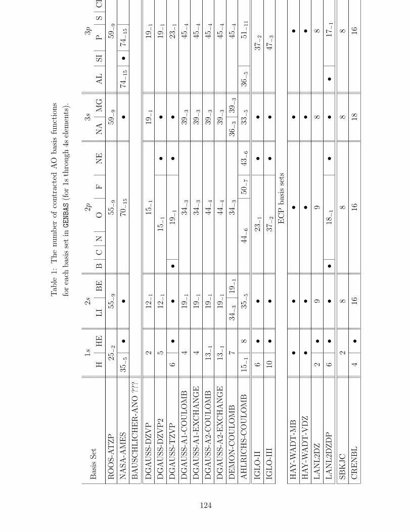
Tab
le1:
The
num
ber
ofco
ntr
acte
dA
Obas
isfu
nct
ions
for
each
bas
isse
tin
GENBAS
(for
1sth
rough
4sel
emen
ts).
Bas
isSet
1s2s
2p3s
3p4s
HH
ELI
BE
BC
NO
FN
EN
AM
GA
LSI
PS
CL
AR
KC
A
RO
OS-A
TZP
25−
255
−9
55−
959
−9
59−
9•
NA
SA
-AM
ES
35−
5•
•70
−15
•74
−15•
74−
15
••
BA
USC
HLIC
HE
R-A
NO
???
DG
AU
SS-D
ZV
P2
12−
115
−1
19−
119
−1
23−
129
−2
DG
AU
SS-D
ZV
P2
512
−1
15−
1•
•19
−1
•D
GA
USS-T
ZV
P6
••
•19
−1
••
23−
1•
DG
AU
SS-A
1-C
OU
LO
MB
419
−1
34−
339
−3
45−
449
−4
DG
AU
SS-A
1-E
XC
HA
NG
E4
19−
134
−3
39−
345
−4
49−
4
DG
AU
SS-A
2-C
OU
LO
MB
13−
119
−1
44−
439
−3
45−
4•
DG
AU
SS-A
2-E
XC
HA
NG
E13
−1
19−
144
−4
39−
345
−4
49−
4
DE
MO
N-C
OU
LO
MB
734
−3
19−
134
−3
36−
339
−3
45−
449
−4
AH
LR
ICH
S-C
OU
LO
MB
15−
18
35−
544
−6
50−
743
−6
33−
536
−5
51−
11
36−
534
−5
IGLO
-II
6•
•23
−1
••
37−
2•
•IG
LO
-III
10•
•37
−2
••
47−
3•
•E
CP
bas
isse
ts
HAY
-WA
DT
-MB
••
••
•5
HAY
-WA
DT
-VD
Z•
••
••
12
LA
NL2D
Z2
•9
98
812
LA
NL2D
ZD
P6
••
•18
−1
••
•17
−1
••
SB
KJC
28
88
88
CR
EN
BL
4•
1616
1816
17
124
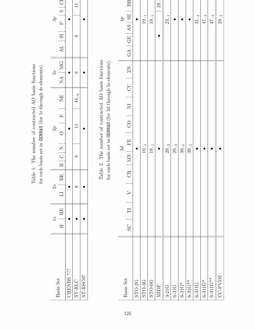
Tab
le1:
The
num
ber
ofco
ntr
acte
dA
Obas
isfu
nct
ions
for
each
bas
isse
tin
GENBAS
(for
1sth
rough
4sel
emen
ts).
Bas
isSet
1s2s
2p3s
3p4s
HH
ELI
BE
BC
NO
FN
EN
AM
GA
LSI
PS
CL
AR
KC
A
CR
EN
BS
???
••
••
••
ST
-RLC
•8
811
44−
68
811
44−
68
ST
-RSC
97•
••
••
1728
−2
Tab
le2:
The
num
ber
ofco
ntr
acte
dA
Obas
isfu
nct
ions
forea
chbas
isse
tin
GENBAS
(for
3dth
rough
5sel
emen
ts).
Bas
isSet
3d4p
5s
SC
TI
VC
RM
NFE
CO
NI
CU
ZN
GA
GE
AS
SE
BR
KR
RB
SR
ST
O-2
G•
••
23−
1
ST
O-3
G19
−1
19−
123
−1
ST
O-6
G19
−1
19−
1•
MID
I!•
•29
−2
••
3-21
G29
−2
23−
127
−1
6-31
G29
−2
••
6-31
G*
39−
5•
•6-
31G
**39
−5
••
6-31
1G•
41−
2•
6-31
1G*
•47
−3
•6-
311G
**•
47−
3•
CC
-PV
DZ
•29
−2
•
125
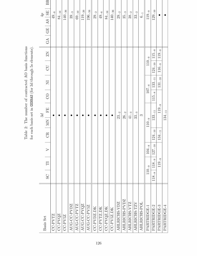
Tab
le2:
The
num
ber
ofco
ntr
acte
dA
Obas
isfu
nct
ions
forea
chbas
isse
tin
GENBAS
(for
3dth
rough
5sel
emen
ts).
Bas
isSet
3d4p
5s
SC
TI
VC
RM
NFE
CO
NI
CU
ZN
GA
GE
AS
SE
BR
KR
RB
SR
CC
-PV
TZ
•49
−6
•C
C-P
VQ
Z•
84−
16
•C
C-P
V5Z
•14
0 −36
•A
UG
-CC
-PV
DZ
•39
−3
•A
UG
-CC
-PV
TZ
•69
−10
•A
UG
-CC
-PV
QZ
•11
9 −26
•A
UG
-CC
-PV
5Z•
196 −
56
•C
C-P
VD
ZD
K•
29−
2•
CC
-PV
TZ
DK
•49
−6
•C
C-P
VQ
ZD
K•
84−
16
•C
C-P
V5Z
DK
•14
0 −36
•A
HLR
ICH
S-V
DZ
23−
229
−2
•A
HLR
ICH
S-P
VD
Z26
−2
35−
3•
AH
LR
ICH
S-V
TZ
41−
338
−2
•A
HLR
ICH
S-T
ZV
33−
333
−2
•A
HLR
ICH
S-P
OL
36 −
1•
PA
RT
RID
GE
-111
0 −9
104 −
811
0 −9
107 −
811
0 −9
119 −
913
2 −10
PA
RT
RID
GE
-211
8 −8
118 −
912
7 −10
124 −
10
133 −
11
115 −
813
3 −11
124 −
10
115 −
812
9 −10
•PA
RT
RID
GE
-311
9 −8
134 −
11
119 −
813
1 −10
116 −
811
9 −8
••
PA
RT
RID
GE
-413
4 −11
••
126

Tab
le2:
The
num
ber
ofco
ntr
acte
dA
Obas
isfu
nct
ions
forea
chbas
isse
tin
GENBAS
(for
3dth
rough
5sel
emen
ts).
Bas
isSet
3d4p
5s
SC
TI
VC
RM
NFE
CO
NI
CU
ZN
GA
GE
AS
SE
BR
KR
RB
SR
WT
BS
16−
119
−1
20−
1
SA
DLE
J-P
VT
Z•
•74
−10
•62
−4
WA
CH
TE
RS+
F60
−7
••
•R
OO
S-A
DZP
65−
10
••
RO
OS-A
TZP
119 −
26
••
NA
SA
-AM
ES
•69
−10
•10
9 −25
•69
−10
••
•B
AU
SC
HLIC
HE
R-A
NO
109 −
25
••
•D
GA
USS-D
ZV
P26
−2
29−
233
−2
39−
3
DG
AU
SS-D
ZV
P2
29−
2•
•D
GA
USS-A
1-C
OU
LO
MB
55−
555
−5
59−
5
DG
AU
SS-A
1-E
XC
HA
NG
E55
−5
55−
559
−5
DG
AU
SS-A
2-C
OU
LO
MB
55−
5•
•D
GA
USS-A
2-E
XC
HA
NG
E55
−5
••
DE
MO
N-C
OU
LO
MB
55−
555
−5
59−
5
AH
LR
ICH
S-C
OU
LO
MB
96−
24
90−
23
96−
24
91−
23
40−
555
−11
56−
11
23−
2SR
68−
15
EC
Pbas
isse
ts
HAY
-WA
DT
-MB
11−
124
−2
••
125
HAY
-WA
DT
-VD
Z24
−2
••
12
LA
NL2D
Z24
−2
20−
28
12
LA
NL2D
ZD
P•
•17
−1
••
SB
KJC
34−
334
−3
88
127
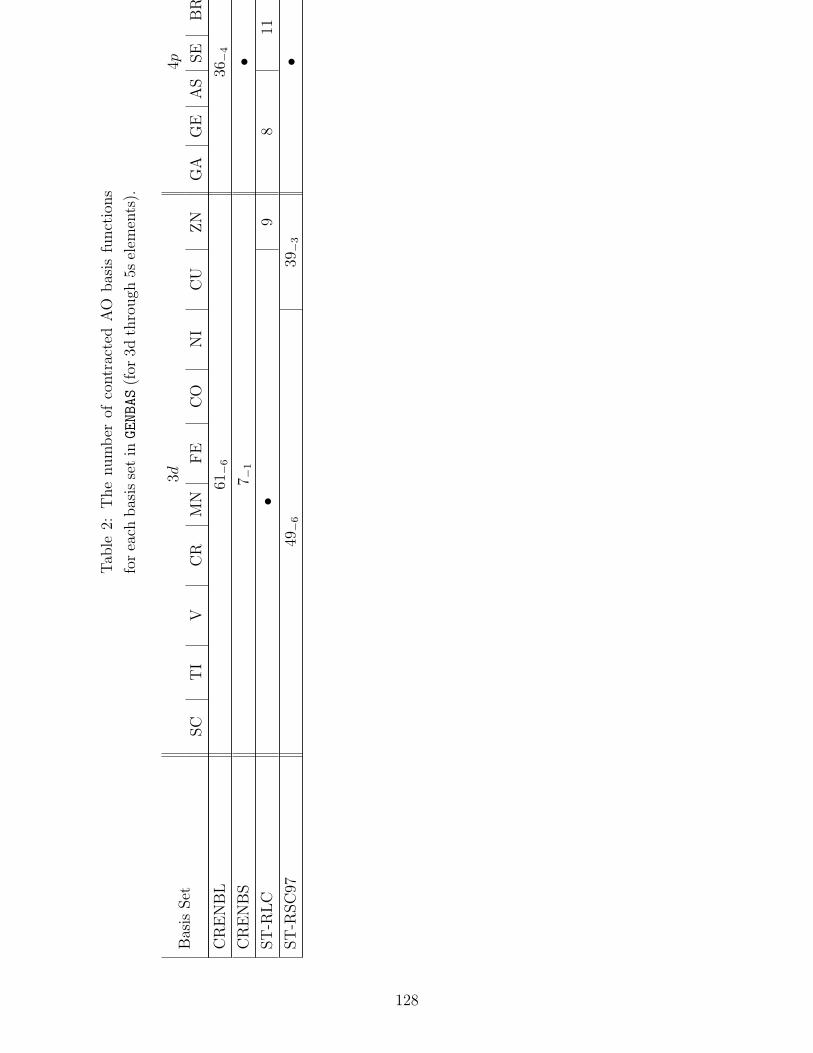
Tab
le2:
The
num
ber
ofco
ntr
acte
dA
Obas
isfu
nct
ions
forea
chbas
isse
tin
GENBAS
(for
3dth
rough
5sel
emen
ts).
Bas
isSet
3d4p
5s
SC
TI
VC
RM
NFE
CO
NI
CU
ZN
GA
GE
AS
SE
BR
KR
RB
SR
CR
EN
BL
61−
636
−4
20
CR
EN
BS
7 −1
••
ST
-RLC
•9
811
44−
68
ST
-RSC
9749
−6
39−
3•
1728
−2
128
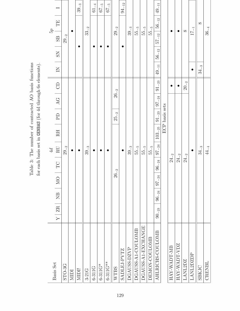
Tab
le3:
The
num
ber
ofco
ntr
acte
dA
Obas
isfu
nct
ions
forea
chbas
isse
tin
GENBAS
(for
4dth
rough
6sel
emen
ts).
Bas
isSet
4d5p
6s
YZR
NB
MO
TC
RU
RH
PD
AG
CD
INSN
SB
TE
IX
EC
SB
A
ST
O-3
G29
−2
29−
2•
•M
IDI
••
31−
2•
MID
I!•
•39
−3
••
3-21
G39
−3
33−
237
−2
•6-
311G
••
61−
4•
•6-
311G
*•
•67
−5
••
6-31
1G**
••
67−
5•
•W
TB
S26
−2
25−
226
−2
29−
230
−2
SA
DLE
J-P
VT
Z•
•94
−12
••
DG
AU
SS-D
ZV
P39
−3
39−
3•
DG
AU
SS-A
1-C
OU
LO
MB
55−
555
−5
•D
GA
USS-A
1-E
XC
HA
NG
E55
−5
55−
5•
DE
MO
N-C
OU
LO
MB
55−
555
−5
•A
HLR
ICH
S-C
OU
LO
MB
90−
23
96−
24
97−
24
96−
24
97−
24
103 −
25
91−
23
97−
24
91−
23
49−
11
56−
12
57−
12
56−
12
49−
11
51−
11
23−
268
−15
EC
Pbas
isse
ts
HAY
-WA
DT
-MB
24−
2•
•12
HAY
-WA
DT
-VD
Z24
−2
••
12
LA
NL2D
Z24
−2
20−
28
12
LA
NL2D
ZD
P•
•17
−1
••
SB
KJC
34−
334
−3
88
CR
EN
BL
44−
436
−4
44−
4
129
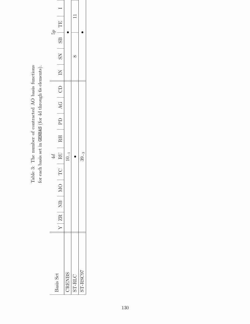
Tab
le3:
The
num
ber
ofco
ntr
acte
dA
Obas
isfu
nct
ions
forea
chbas
isse
tin
GENBAS
(for
4dth
rough
6sel
emen
ts).
Bas
isSet
4d5p
6s
YZR
NB
MO
TC
RU
RH
PD
AG
CD
INSN
SB
TE
IX
EC
SB
A
CR
EN
BS
10−
1•
•ST
-RLC
•8
1144
−6
8
ST
-RSC
9739
−3
•17
38−
5
130

B.2 ECP sets in ECPDATA
131
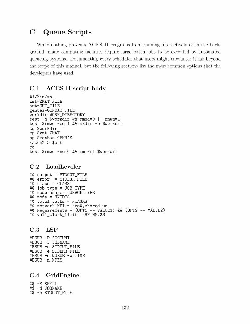
C Queue Scripts
While nothing prevents ACES II programs from running interactively or in the back-
ground, many computing facilities require large batch jobs to be executed by automated
queueing systems. Documenting every scheduler that users might encounter is far beyond
the scope of this manual, but the following sections list the most common options that the
developers have used.
C.1 ACES II script body
#!/bin/shzmt=ZMAT_FILEout=OUT_FILEgenbas=GENBAS_FILEworkdir=WORK_DIRECTORYtest -d $workdir && rmwd=0 || rmwd=1test $rmwd -eq 1 && mkdir -p $workdircd $workdircp $zmt ZMATcp $genbas GENBASxaces2 > $outcd -test $rmwd -ne 0 && rm -rf $workdir
C.2 LoadLeveler
#@ output = STDOUT_FILE#@ error = STDERR_FILE#@ class = CLASS#@ job_type = JOB_TYPE#@ node_usage = USAGE_TYPE#@ node = NNODES#@ total_tasks = NTASKS#@ network.MPI = css0,shared,us#@ Requirements = (OPT1 == VALUE1) && (OPT2 == VALUE2)#@ wall_clock_limit = HH:MM:SS
C.3 LSF
#BSUB -P ACCOUNT#BSUB -J JOBNAME#BSUB -o STDOUT_FILE#BSUB -e STDERR_FILE#BSUB -q QUEUE -W TIME#BSUB -n NPES
C.4 GridEngine
#$ -S SHELL#$ -N JOBNAME#$ -o STDOUT_FILE
132

#$ -e STDERR_FILE#$ -l COMPLEX#$ -pe PE_ENV NPES
133
Index
*ACES2
ABCDFULL, 56
ABCDTYPE, 55, 56, 57
ACC SYM, 59
AO LADDERS, 55
BASIS, 46
BRUCK CONV, 53
BRUECKNER, 53
CACHE RECS, 45
CALCLEVEL, 43
CC CONV, 57
CC EXPORDER, 57
CC EXTRAPOL, 57
CC MAXCYC, 57
CCR12, 111
CHARGE, 46
CHECK SYM, 49
CONTRACTION, 47
CONVERGENCE, 67
COORDINATES, 46
CPHF CONVER, 65
CPHF MAXCYC, 65
CURVILINEAR, 66
DAMP TOL, 51
DAMP TYP, 51
DAMPSCF, 51
DEA CALC, 60
DEA SYM, 60
DENSITY, 58
DERIV LEV, 44
DIP CALC, 62
DIP SYM, 63
DIRECT, 47
DOHBAR, 58
DROPMO, 52
EA CALC, 60
EA SYM, 60
ECP, 47
EE SEARCH, 61
EE SYM, 61
EIGENVECTOR, 66
EOM MAXC, 58
EOM PRJCT, 59
EOMPROP, 64
EOMREF, 58
EOMXFIELD, 111
EOMYFIELD, 111
EOMZFIELD, 111
ESTATE MAXC, 58
ESTATE PROP, 59
ESTATE SYM, 61
ESTATE TOL, 58
EVAL HESS, 67
EXCITE, 58
EXTERNAL, 69
FD IRREPS, 68
FD PROJECT, 69
FD STEPSIZE, 68
FD USEGROUP, 69
FILE RECSIZ, 45
FILE STRIPE, 111
FOCK, 49
FUNCTIONAL, 111
GAMMA ABCD, 56
GENBAS 1, 46
GENBAS 2, 47
GENBAS 3, 47
GEOM OPT, 66
GLOBAL MEM, 111
GRAD CALC, 44
134
GUESS, 49
HBARABCD, 56
HBARABCI, 56
HESS UPDATE, 67
HF2 FILE, 55, 56
HFSTABILITY, 52, 58
IMEM SIZE, 59
INCORE, 45
INIT HESSIAN, 67
INSERTF, 111
INTEGRALS, 47
INTGRL TOL, 47
IP CALC, 62
IP SEARCH, 62
IP SYM, 62
JODA PRINT, 45
KS POT, 111
KUCHARSKI, 111
LINDEP TOL, 46
LOCK ORBOCC, 50
LSHF A1, 52
LSHF B1, 52
MAKERHF, 55
MAX STEP, 66
MEMORY SIZE, 43, 45
MULTIPLICITY, 46
NEGEVAL, 67
NEWVRT, 50
NONHF, 48
NOREORI, 45
NT2EOMEE, 59
NTOP TAMP, 57
OCCUPATION, 50, 50
OPT MAXCYC, 67
OPT METHOD, 66
ORBITALS, 48
ORDER RLE, see CC EXPORDER
PERT ORB, 48
POINTS, 69
POLYRATE, 111
PRINT, 45
PROGRAM, 58
PROPS, 64
PRP INTS, 65
PSI, 111
QRHF GENERAL, 53
QRHF ORBITAL, 54
QRHF SPIN, 54
RAMAN, 68
RDO, 111
REFERENCE, 48
RESET FLAGS, 111
RESRAMAN, 63
RESTART, 43
RLE, see CC EXTRAPOL
ROT EVEC, 52
RPP, see SCF EXTRAP
RPP LATEST, see SCF EXPSTAR
RPP ORDER, see SCF EXPORDER
SAVE INTS, 55
SCF CONV, 51
SCF EXPORDER, 51
SCF EXPSTAR, 52
SCF EXTRAP, 51
SCF MAXCYC, 51
SCF PRINT, 49
SCF TYPE, 49, 112
SINGLE STORE, 55
SOLVENT, 111
SPHERICAL, 46
STP SIZ CTL, 66
SUBGROUP, 44
SUBGRPAXIS, 44
SYMMETRY, 44
135
TAMP SUM, 57
TDHF, 64
TRANS INV, 68
TREAT PERT, 65
TURBOMOLE, 111
UNITS, 46
UNO CHARGE, 54
UNO MULT, 55
UNO REF, 54
VIBRATION, 68
VTRAN, 56
XFIELD, 65
XFORM TOL, 57
YFIELD, 65
ZETA CONV, 63
ZETA MAXCYC, 63
ZETA TYPE, 63
ZFIELD, 65
*INTGRT
CUTOFF, 113
ENEGRID, 113
ENETYPE, 113
EXACT EX, 113
FUNC, 113
FUZZYITER, 112
KSPOT, 113
NUMACC, 112
PARTPOLY, 112
PARTTYP, 112
POTGRID, 113
POTRADPTS, 112
POTTYPE, 113
RADLIMIT, 112
RADSCAL, 112
RADTYP, 112
TDKS, 113
*VSCF
KS, 112
136