Embed Size (px)
Citation preview
A Study of Variable Thrust, Variable Isp
Trajectories for Solar System Exploration
A ThesisPresented to
The Academic Faculty
by
Tadashi Sakai
In Partial Fulfillmentof the Requirements for the Degree
Doctor of Philosophy
School of Aerospace EngineeringGeorgia Institute of Technology
October 2004
A Study of Variable Thrust, Variable Isp
Trajectories for Solar System Exploration
Approved by:
John R. Olds, Advisor
Robert D. Braun
Eric N. Johnson
Amy R. Pritchett
David W. Way
Date Approved

To Naomi
iii
ACKNOWLEDGEMENTS
There are many people whom I would like to thank. First, I would like to express my
sincere gratitude and thanks to my graduate advisor Dr. John Olds. It has been a privilege
to work with you. Without your guidance, wisdom, encouragement, and patience, this
research would have not been possible.
I would also like to thank the other members of my committee, Dr. Robert Braun, Dr.
Eric Johnson, Dr. Amy Pritchett, and Dr. David Way. Your advice and insight has proved
invaluable. I would also like to thank Dr. Panagiotis Tsiotras for his advice.
Thank you also to my friends and coworkers in the Space Systems Design Lab. I really
had a great time working with you. Especially I would like to thank Tim Kokan, David
Young, Jimmy Young, and Kristina Alemany for their proofreading of this thesis. Reading
and correcting my English must have been tough work. Other than the members of SSDL,
Yoko Watanabe’s knowledge and comments were really helpful. I hope their research will
be fruitful and successful.
I would like to thank my family in Japan. My father Toshio, mother Takae, elder brother
Hiroshi, and younger sister Maki; they have all supported me so much. I can not thank you
enough.
Finally, I must thank my wife, Naomi, who has provided endless encouragement and
support during the most difficult times of my work. Having you in my life to share my
dreams and experiences makes them all the more special.
iv
TABLE OF CONTENTS
DEDICATION iii
ACKNOWLEDGEMENTS iv
LIST OF TABLES ix
LIST OF FIGURES xi
LIST OF SYMBOLS OR ABBREVIATIONS xvi
SUMMARY xviii
I INTRODUCTION 1
1.1 Problems of Variable Thrust, Variable Isp Trajectory Optimization . . . . 1
1.2 Motivation for Research . . . . . . . . . . . . . . . . . . . . . . . . . . . . 3
1.3 Research Goals and Objectives . . . . . . . . . . . . . . . . . . . . . . . . . 5
1.4 Approach . . . . . . . . . . . . . . . . . . . . . . . . . . . . . . . . . . . . . 6
1.5 Organization of the Thesis . . . . . . . . . . . . . . . . . . . . . . . . . . . 7
II A BRIEF DESCRIPTION OF LOW THRUST TRAJECTORY OPTI-MIZATION 9
2.1 Trajectory Optimization in General . . . . . . . . . . . . . . . . . . . . . . 9
2.2 Solution Methods for Optimization Problems . . . . . . . . . . . . . . . . . 9
2.3 Indirect Methods – Calculus of Variations . . . . . . . . . . . . . . . . . . 11
2.3.1 Problems without Terminal Constraints, Fixed Terminal Time . . . 11
2.3.2 Some State Variables Specified at a Fixed Terminal Time . . . . . 12
2.3.3 Inequality Constraints on the Control Variables . . . . . . . . . . . 15
2.3.4 Bang-off-bang Control . . . . . . . . . . . . . . . . . . . . . . . . . 15
2.4 Literature Review . . . . . . . . . . . . . . . . . . . . . . . . . . . . . . . . 17
III EXHAUST-MODULATED PLASMA PROPULSION SYSTEMS 21
3.1 Overview . . . . . . . . . . . . . . . . . . . . . . . . . . . . . . . . . . . . . 21
3.2 Mechanism . . . . . . . . . . . . . . . . . . . . . . . . . . . . . . . . . . . . 23
3.3 Choosing the Power Level . . . . . . . . . . . . . . . . . . . . . . . . . . . 26
v
IV PRELIMINARY STUDY: COMPARISON OF HIGH THRUST, CON-STANT ISP , AND VARIABLE ISP WITH SIMPLE TRAJECTORIES 29
4.1 Problem Formulation . . . . . . . . . . . . . . . . . . . . . . . . . . . . . . 29
4.2 Results . . . . . . . . . . . . . . . . . . . . . . . . . . . . . . . . . . . . . . 32
V INTERPLANETARY TRAJECTORY OPTIMIZATION PROBLEMS 38
5.1 Assumptions . . . . . . . . . . . . . . . . . . . . . . . . . . . . . . . . . . . 38
5.2 Equations of Motion for Low Thrust Trajectories . . . . . . . . . . . . . . 43
5.2.1 VSI – No Constraints on Isp . . . . . . . . . . . . . . . . . . . . . . 43
5.2.2 VSI – Inequality Constraints on Isp . . . . . . . . . . . . . . . . . . 44
5.2.3 CSI – Continuous Thrust . . . . . . . . . . . . . . . . . . . . . . . . 45
5.2.4 CSI – Bang-Off-Bang Control . . . . . . . . . . . . . . . . . . . . . 46
5.3 Solving the High Thrust Trajectory . . . . . . . . . . . . . . . . . . . . . . 47
5.4 Problems with Swing-by . . . . . . . . . . . . . . . . . . . . . . . . . . . . 50
5.4.1 Mechanism . . . . . . . . . . . . . . . . . . . . . . . . . . . . . . . . 50
5.4.2 Equations of Motion . . . . . . . . . . . . . . . . . . . . . . . . . . 51
5.4.3 Powered Swing-by . . . . . . . . . . . . . . . . . . . . . . . . . . . . 55
VI DEVELOPMENT OF THE APPLICATION “SAMURAI” 57
6.1 Overview . . . . . . . . . . . . . . . . . . . . . . . . . . . . . . . . . . . . . 57
6.1.1 Capabilities . . . . . . . . . . . . . . . . . . . . . . . . . . . . . . . 57
6.1.2 Performance Index for Each Engine . . . . . . . . . . . . . . . . . . 60
6.2 C++ Classes . . . . . . . . . . . . . . . . . . . . . . . . . . . . . . . . . . . 61
6.3 Flow and Schemes . . . . . . . . . . . . . . . . . . . . . . . . . . . . . . . . 65
6.3.1 SAMURAI Flowchart . . . . . . . . . . . . . . . . . . . . . . . . . . 65
6.3.2 VSI Constrained Isp . . . . . . . . . . . . . . . . . . . . . . . . . . 67
6.3.3 CSI Continuous Thrust . . . . . . . . . . . . . . . . . . . . . . . . . 68
6.3.4 CSI Bang-Off-Bang . . . . . . . . . . . . . . . . . . . . . . . . . . . 68
6.4 Examples of Input and Output . . . . . . . . . . . . . . . . . . . . . . . . 70
6.5 Validation and Verification . . . . . . . . . . . . . . . . . . . . . . . . . . . 75
6.5.1 Validation of High Thrust with IPREP . . . . . . . . . . . . . . . . 75
6.5.2 Validation of CSI with ChebyTOP . . . . . . . . . . . . . . . . . . 75
vi
VII PRELIMINARY RESULTS: PROOF OF CONCEPT 80
7.1 Problem Description . . . . . . . . . . . . . . . . . . . . . . . . . . . . . . 80
7.2 Numerical Accuracy . . . . . . . . . . . . . . . . . . . . . . . . . . . . . . . 82
7.3 Results and Discussion . . . . . . . . . . . . . . . . . . . . . . . . . . . . . 84
7.4 Relationship among Fuel Consumption, Jet Power, and Travel Distance . . 93
VIIINUMERICAL EXAMPLES: “REAL WORLD” PROBLEMS 100
8.1 Scientific Mission to Venus . . . . . . . . . . . . . . . . . . . . . . . . . . . 101
8.1.1 Venus Exploration . . . . . . . . . . . . . . . . . . . . . . . . . . . 101
8.1.2 Problem Description . . . . . . . . . . . . . . . . . . . . . . . . . . 101
8.1.3 Results . . . . . . . . . . . . . . . . . . . . . . . . . . . . . . . . . . 101
8.2 Human Mission to Mars: Round Trip . . . . . . . . . . . . . . . . . . . . . 109
8.2.1 Mars Exploration . . . . . . . . . . . . . . . . . . . . . . . . . . . . 109
8.2.2 Problem Description . . . . . . . . . . . . . . . . . . . . . . . . . . 110
8.2.3 Results . . . . . . . . . . . . . . . . . . . . . . . . . . . . . . . . . . 110
8.3 JIMO: Jupiter Icy Moons Orbiter . . . . . . . . . . . . . . . . . . . . . . . 121
8.3.1 JIMO Overview . . . . . . . . . . . . . . . . . . . . . . . . . . . . . 121
8.3.2 Problem Description . . . . . . . . . . . . . . . . . . . . . . . . . . 122
8.3.3 Results . . . . . . . . . . . . . . . . . . . . . . . . . . . . . . . . . . 122
8.4 Uranus and beyond . . . . . . . . . . . . . . . . . . . . . . . . . . . . . . . 127
8.5 Swing-by Trajectories with Mars . . . . . . . . . . . . . . . . . . . . . . . . 129
IX CONCLUSIONS AND RECOMMENDED FUTURE WORK 138
9.1 Conclusions and Observations . . . . . . . . . . . . . . . . . . . . . . . . . 139
9.2 Research Accomplishments . . . . . . . . . . . . . . . . . . . . . . . . . . . 141
9.3 Recommended Future Work . . . . . . . . . . . . . . . . . . . . . . . . . . 142
APPENDIX A — ADDITIONAL RESULTS FROM PRELIMINARY STUDY144
APPENDIX B — EQUATIONS USED IN THE CODE 155
APPENDIX C — NUMERICAL TECHNIQUES 159
APPENDIX D — “SAMURAI” CODE MANUAL 177
REFERENCES 180
vii

VITA 186
viii
LIST OF TABLES
1 Examples of Spacecraft Propulsion Systems[4][42]. . . . . . . . . . . . . . . 1
2 Trip Time Savings(Comparison by Distance): (VSI - CSI)/CSI × 100 (%) . 37
3 Trip Time Savings(Comparison by Initial Mass): (VSI - CSI)/CSI × 100 (%) 37
4 Orbital Data[37]. . . . . . . . . . . . . . . . . . . . . . . . . . . . . . . . . . 81
5 Transfer Orbit to Venus with 10MW Jet Power. . . . . . . . . . . . . . . . . 85
6 Transfer Orbit to Saturn with 30MW Jet Power. . . . . . . . . . . . . . . . 86
7 Time Until Spacecraft Mass (m0 = 100MT) Becomes Zero (in TU Sun). . . 86
8 Fuel Consumption for VSI type II and CSI type I (kg). . . . . . . . . . . . . 89
9 Earth – Mars Round Trip Fuel Consumption for VSI type I . . . . . . . . . 110
10 Earth – Mars Round Trip Fuel Consumption . . . . . . . . . . . . . . . . . 114
11 Comparison of High Thrust ∆V for Earth – Jupiter: With and Without MarsSwing-by . . . . . . . . . . . . . . . . . . . . . . . . . . . . . . . . . . . . . 130
12 Comparison of High Thrust ∆V for Earth – Saturn: With and Without MarsSwing-by . . . . . . . . . . . . . . . . . . . . . . . . . . . . . . . . . . . . . 130
13 Comparison of Fuel Consumption for VSI type I: from Earth to Jupiter Withand Without Mars Swing-by . . . . . . . . . . . . . . . . . . . . . . . . . . . 133
14 Comparison of Fuel Consumption for VSI type I: from Earth to Saturn Withand Without Mars Swing-by . . . . . . . . . . . . . . . . . . . . . . . . . . . 133
15 Comparison of Fuel Consumption for VSI type II: from Earth to JupiterWith and Without Mars Swing-by . . . . . . . . . . . . . . . . . . . . . . . 135
16 Comparison of Fuel Consumption for VSI type II: from Earth to Saturn Withand Without Mars Swing-by . . . . . . . . . . . . . . . . . . . . . . . . . . . 135
17 Comparison of Fuel Consumption for CSI type II: from Earth to Jupiter Withand Without Mars Swing-by . . . . . . . . . . . . . . . . . . . . . . . . . . . 136
18 Comparison of Fuel Consumption for CSI type II: from Earth to Saturn Withand Without Mars Swing-by . . . . . . . . . . . . . . . . . . . . . . . . . . . 136
19 Transfer Orbit to Venus with 20MW Jet Power. . . . . . . . . . . . . . . . . 144
20 Transfer Orbit to Venus with 30MW Jet Power. . . . . . . . . . . . . . . . . 145
21 Transfer Orbit to Mars with 10MW Jet Power. . . . . . . . . . . . . . . . . 146
22 Transfer Orbit to Mars with 20MW Jet Power. . . . . . . . . . . . . . . . . 147
23 Transfer Orbit to Mars with 30MW Jet Power. . . . . . . . . . . . . . . . . 148
24 Transfer Orbit to Asteroids with 10MW Jet Power. . . . . . . . . . . . . . . 149
ix
25 Transfer Orbit to Asteroids with 20MW Jet Power. . . . . . . . . . . . . . . 150
26 Transfer Orbit to Asteroids with 30MW Jet Power. . . . . . . . . . . . . . . 151
27 Transfer Orbit to Jupiter with 10MW Jet Power. . . . . . . . . . . . . . . . 152
28 Transfer Orbit to Jupiter with 20MW Jet Power. . . . . . . . . . . . . . . . 152
29 Transfer Orbit to Jupiter with 30MW Jet Power. . . . . . . . . . . . . . . . 153
30 Transfer Orbit to Saturn with 10MW Jet Power. . . . . . . . . . . . . . . . 153
31 Transfer Orbit to Saturn with 20MW Jet Power. . . . . . . . . . . . . . . . 154
x
LIST OF FIGURES
1 Future Interplanetary Flight with VASIMR[5]. . . . . . . . . . . . . . . . . 3
2 Transfer Trajectory from Earth to Mars with Thrust Direction. . . . . . . . 4
3 Bang-off-bang Control: Choosing Control to Minimize qi. . . . . . . . . . . 17
4 VX-10 Experiment at Johnson Space Center[45]. . . . . . . . . . . . . . . . 22
5 Synoptic View of the VASIMR Engine[22]. . . . . . . . . . . . . . . . . . . . 24
6 Power Partitioning and Relationship between Thrust and Isp. . . . . . . . . 25
7 Thrust vs. Mass Flow Rate for a CSI Engine. . . . . . . . . . . . . . . . . . 27
8 Thrust vs. Mass Flow Rate for a VSI Engine. . . . . . . . . . . . . . . . . . 27
9 Thrust vs. Mass Flow Rate for a VSI Engine with Limitations. . . . . . . . 28
10 Trajectories for Preliminary Study. . . . . . . . . . . . . . . . . . . . . . . . 29
11 Preliminary Study: Isp for VSI and CSI. . . . . . . . . . . . . . . . . . . . . 30
12 Results: R = 100 DU, m0 = 20 MT, PJ = 500 kW. . . . . . . . . . . . . . 32
13 Isp histories for VSI and CSI when CSI Isp is 3,000 sec: R = 100 DU, m0 =20 MT, PJ = 500 kW. . . . . . . . . . . . . . . . . . . . . . . . . . . . . . . 33
14 Results: R = 500 DU, m0 = 20 MT, PJ = 500 kW. . . . . . . . . . . . . . 34
15 Results R = 1,000 DU, m0 = 20 MT, PJ = 500 kW. . . . . . . . . . . . . . 35
16 Results: R = 100 DU, m0 = 5 MT, PJ = 500 kW. . . . . . . . . . . . . . . 36
17 Results: R = 100 DU, m0 = 10 MT, PJ = 500 kW. . . . . . . . . . . . . . 36
18 Sphere of Influence of m2 with respect to m1. . . . . . . . . . . . . . . . . . 39
19 In-plane Thrust Angle θ and Out-of-plane Thrust Angle φ in Inertial Frame. 46
20 Switching Function and Switching Times for Bang-Off-Bang. . . . . . . . . 47
21 Gauss Problem: Direction of Motion for the Same Vectors and the SameTime of Flight. . . . . . . . . . . . . . . . . . . . . . . . . . . . . . . . . . . 48
22 Schematic Diagram of Forming of Gravity Assist Maneuver. . . . . . . . . . 52
23 Swing-by: Inside the SOI. . . . . . . . . . . . . . . . . . . . . . . . . . . . . 53
24 Geometry of a Powered Swing-by Maneuver. . . . . . . . . . . . . . . . . . . 55
25 Examples of Thrust Histories. . . . . . . . . . . . . . . . . . . . . . . . . . . 59
26 SAMURAI Flowchart. . . . . . . . . . . . . . . . . . . . . . . . . . . . . . . 64
27 Input C3 and ∆V requirements. . . . . . . . . . . . . . . . . . . . . . . . . . 66
xi
28 α (in-plane thrust angle) and β (out-of-plane thrust angle) in the Spacecraft-centered Coordinates. . . . . . . . . . . . . . . . . . . . . . . . . . . . . . . 71
29 Results with SAMURAI and IPREP: ∆V Requirements for High ThrustVenus Transfer. . . . . . . . . . . . . . . . . . . . . . . . . . . . . . . . . . . 76
30 Results with SAMURAI and IPREP: ∆V Requirements for High ThrustMars Transfer. . . . . . . . . . . . . . . . . . . . . . . . . . . . . . . . . . . 76
31 Results with SAMURAI and IPREP: ∆V Requirements for High ThrustJupiter Transfer. . . . . . . . . . . . . . . . . . . . . . . . . . . . . . . . . . 77
32 Results with SAMURAI and ChebyTOP: ∆V Requirements for CSI type IMars Transfer. . . . . . . . . . . . . . . . . . . . . . . . . . . . . . . . . . . 78
33 Results with SAMURAI and ChebyTOP: ∆V Requirements for CSI type IIMars Transfer. . . . . . . . . . . . . . . . . . . . . . . . . . . . . . . . . . . 79
34 2D Trajectories for Proof-of-Concept Problems. . . . . . . . . . . . . . . . . 81
35 Tolerance vs. CPU Time for Different Number of Time Steps. . . . . . . . . 83
36 Tolerance vs. Fuel Consumption for Different Number of Time Steps. . . . 84
37 A Trajectory with More Than One Revolution - CSI type I engine. . . . . . 88
38 A Trajectory with Long Time of Flight - VSI type I engine. . . . . . . . . . 89
39 VSI type II: Thrust History for Different Levels of Isp Limit. . . . . . . . . 90
40 VSI type II: Isp History for Different Levels of Isp Limit. . . . . . . . . . . . 91
41 VSI type II: Fuel Consumption for Different Levels of Isp Limit. . . . . . . . 92
42 CSI type II: Thrust History for Different Levels of Isp. . . . . . . . . . . . . 92
43 CSI type II: Isp History for Different Levels of Isp. . . . . . . . . . . . . . . 93
44 CSI type II: Fuel Consumption for Different Levels of Isp. . . . . . . . . . . 94
45 Relative Fuel Consumption of VSI with respect to CSI: Comparison by JetPower. . . . . . . . . . . . . . . . . . . . . . . . . . . . . . . . . . . . . . . . 95
46 Relative Fuel Consumption of VSI with respect to CSI: Comparison by Dis-tance from the Sun (The Best Isp is Chosen for Each CSI Mission). . . . . . 96
47 Relative Fuel Consumption of VSI with respect to CSI: Comparison by Dis-tance from the Sun (Isp for CSI is the Same for All Missions). . . . . . . . . 97
48 Fuel Consumption between VSI and CSI: When Isp for CSI Differs for EachMission. . . . . . . . . . . . . . . . . . . . . . . . . . . . . . . . . . . . . . . 98
49 Fuel Consumption between VSI and CSI: When Isp for All CSI Cases Arethe Same. . . . . . . . . . . . . . . . . . . . . . . . . . . . . . . . . . . . . . 98
50 Fuel Consumption for VSI type II: Earth – Venus. . . . . . . . . . . . . . . 102
51 Trajectory from Earth to Venus with 160-day Time of Flight. . . . . . . . . 103
xii
52 Fuel Consumption for VSI type II: Earth – Venus. . . . . . . . . . . . . . . 103
53 VSI type II Trajectory from Earth to Venus with 90-day Time of Flight. . . 104
54 Thrust Steering Angle for VSI type II: Earth to Venus, 90-day Time of Flight.105
55 Thrust Magnitude and Isp for VSI type II: Earth to Venus, 90-day Time ofFlight. . . . . . . . . . . . . . . . . . . . . . . . . . . . . . . . . . . . . . . . 105
56 Fuel Consumption for CSI type I: Earth – Venus. . . . . . . . . . . . . . . . 106
57 CSI Type I Trajectory from Earth to Venus with 90-day Time of Flight. . . 106
58 Thrust Steering Angle for CSI type I: Earth – Venus, Day 250, 90 day TOF. 107
59 Thrust Magnitude and Isp for CSI type I: Earth – Venus, Day 250, 90 dayTOF. . . . . . . . . . . . . . . . . . . . . . . . . . . . . . . . . . . . . . . . 107
60 CSI Type II Trajectory from Earth to Venus with 90-day Time of Flight. . 107
61 Thrust Steering Angle for CSI type II: Earth – Venus, Day 260, 90 day TOF. 108
62 Thrust Magnitude and Isp for CSI type II: Earth – Venus, Day 260, 90 dayTOF. . . . . . . . . . . . . . . . . . . . . . . . . . . . . . . . . . . . . . . . 108
63 Fuel Consumption for High Thrust: Earth – Venus. . . . . . . . . . . . . . . 108
64 Fuel Consumption for VSI type I, 10 MW Jet Power: Earth – Mars Outbound.111
65 Fuel Consumption for VSI type I, 10MW Jet Power: Earth – Mars Inbound. 111
66 Fuel Consumption for VSI type II: Earth – Mars Outbound. . . . . . . . . . 112
67 Fuel Consumption for VSI type II: Mars – Earth Inbound. . . . . . . . . . . 112
68 Fuel Consumption for CSI type I: Earth – Mars Outbound. . . . . . . . . . 113
69 Fuel Consumption for CSI type I: Earth – Mars Inbound. . . . . . . . . . . 113
70 Fuel Consumption for CSI type II: Earth – Mars Outbound. . . . . . . . . . 113
71 Fuel Consumption for CSI type II: Mars – Earth Inbound. . . . . . . . . . . 113
72 Fuel Consumption for High Thrust: Earth – Mars Outbound. . . . . . . . . 114
73 Fuel Consumption for High Thrust: Earth – Mars Inbound. . . . . . . . . . 114
74 VSI Type II Trajectory from Earth to Mars with 120-day Time of Flight. . 115
75 Thrust Steering Angle for VSI type II: Earth – Mars Outbound. . . . . . . 116
76 Thrust Magnitude and Isp for VSI type II: Earth – Mars Outbound. . . . . 116
77 Thrust Steering Angle for VSI type II: Mars – Earth Inbound. . . . . . . . 116
78 Thrust Magnitude and Isp for VSI type II: Mars – Earth Inbound. . . . . . 116
79 CSI Type I Trajectory from Earth to Mars with 120-day Time of Flight. . . 117
80 CSI Type II Trajectory from Earth to Mars with 120-day Time of Flight. . 118
xiii
81 Thrust Steering Angle for CSI type II: Mars – Earth Outbound. . . . . . . 119
82 Thrust Magnitude and Isp for CSI type II: Mars – Earth Outbound. . . . . 119
83 Thrust Steering Angle for CSI type II: Mars – Earth Inbound. . . . . . . . 119
84 Thrust Magnitude and Isp for CSI type II: Mars – Earth Inbound. . . . . . 119
85 JIMO: Jupiter Icy Moons Orbiter [3]. . . . . . . . . . . . . . . . . . . . . . 121
86 Fuel Consumption for VSI type I: Earth – Jupiter. . . . . . . . . . . . . . . 122
87 Fuel Consumption for VSI type II: Earth – Jupiter. . . . . . . . . . . . . . . 123
88 Fuel Consumption for CSI type I: Earth – Jupiter. . . . . . . . . . . . . . . 124
89 Transfer Trajectory for VSI type II: Earth – Jupiter. . . . . . . . . . . . . . 125
90 Thrust Steering Angle for VSI type II: Earth – Jupiter, 365-day TOF. . . . 125
91 Thrust Magnitude and Isp for VSI type II: Earth – Jupiter, 365-day TOF. . 125
92 Transfer Trajectory for CSI type I: Earth – Jupiter. . . . . . . . . . . . . . 125
93 Thrust Steering Angle for CSI type I: Earth – Jupiter, 365-day TOF. . . . . 126
94 Thrust Magnitude and Isp for CSI type I: Earth – Jupiter, 365-day TOF. . 126
95 Transfer Trajectory for CSI type II: Earth – Jupiter. . . . . . . . . . . . . . 126
96 Thrust Steering Angle for CSI type II: Earth – Jupiter, 365-day TOF. . . . 126
97 Thrust Magnitude and Isp for CSI type II: Earth – Jupiter, 365-day TOF. . 126
98 Transfer Trajectory for VSI type II: Earth – Uranus. . . . . . . . . . . . . . 128
99 Departure Phase of Transfer Trajectory for VSI type II: Earth – Uranus. . . 128
100 Transfer Trajectory for CSI type I: Earth – Uranus. . . . . . . . . . . . . . 128
101 Departure Phase of Transfer Trajectory for CSI type I: Earth – Uranus. . . 128
102 Transfer Trajectory for CSI type II: Earth – Uranus. . . . . . . . . . . . . . 129
103 Departure Phase of Transfer Trajectory for CSI type II: Earth – Uranus. . . 129
104 Transfer Trajectory for High Thrust: Earth to Saturn without Swing-by. . . 131
105 Transfer Trajectory for High Thrust: Earth to Saturn with Mars Swing-by. 131
106 Transfer Trajectory for VSI type I: Earth to Jupiter without Swing-by. . . . 132
107 Transfer Trajectory for VSI type I: Earth to Jupiter with Mars Swing-by. . 132
108 Transfer Trajectory for VSI type I: Earth to Saturn without Swing-by. . . . 132
109 Transfer Trajectory for VSI type I: Earth to Saturn with Mars Swing-by. . 132
110 Transfer Trajectory for VSI type II: Earth to Jupiter without Swing-by. . . 133
111 Transfer Trajectory for VSI type II: Earth to Jupiter with Mars Swing-by. . 133
xiv
112 Transfer Trajectory for VSI type II: Earth to Saturn without Swing-by. . . 134
113 Transfer Trajectory for VSI type II: Earth to Saturn with Mars Swing-by. . 134
114 Transfer Trajectory for CSI type II: Earth to Jupiter without Swing-by. . . 134
115 Transfer Trajectory for CSI type II: Earth to Jupiter with Mars Swing-by. . 134
116 Transfer Trajectory for CSI type II: Earth to Saturn without Swing-by. . . 134
117 Transfer Trajectory for CSI type II: Earth to Saturn with Mars Swing-by. . 134
118 Specific Energy for Swing-by Trajectory: Earth – Mars – Jupiter. . . . . . . 136
119 Specific Energy for Swing-by Trajectory: Earth – Mars – Saturn. . . . . . . 137
120 Example of Fuel vs. Time of Flight for VSI type I. . . . . . . . . . . . . . . 140
121 Flowchart of Powell’s method[78]. . . . . . . . . . . . . . . . . . . . . . . . . 164
122 Example of Exterior Penalty Function [78]. . . . . . . . . . . . . . . . . . . 170
123 Example of Interior Penalty Function [78]. . . . . . . . . . . . . . . . . . . . 171
124 Example of Extended Penalty Function [78]. . . . . . . . . . . . . . . . . . . 172
125 VRML Example – Simple House. . . . . . . . . . . . . . . . . . . . . . . . . 174
xv
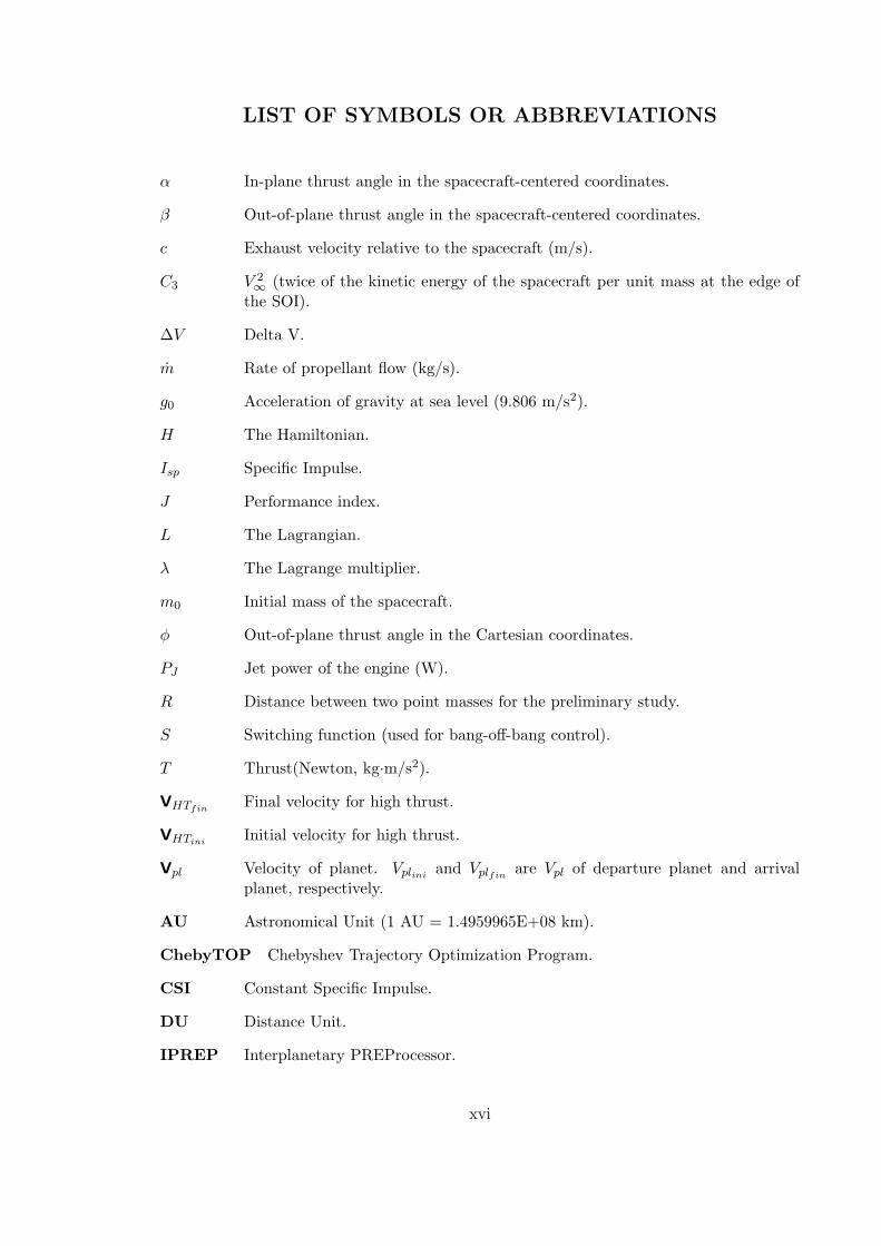
LIST OF SYMBOLS OR ABBREVIATIONS
α In-plane thrust angle in the spacecraft-centered coordinates.
β Out-of-plane thrust angle in the spacecraft-centered coordinates.
c Exhaust velocity relative to the spacecraft (m/s).
C3 V 2∞
(twice of the kinetic energy of the spacecraft per unit mass at the edge ofthe SOI).
∆V Delta V.
m Rate of propellant flow (kg/s).
g0 Acceleration of gravity at sea level (9.806 m/s2).
H The Hamiltonian.
Isp Specific Impulse.
J Performance index.
L The Lagrangian.
λ The Lagrange multiplier.
m0 Initial mass of the spacecraft.
φ Out-of-plane thrust angle in the Cartesian coordinates.
PJ Jet power of the engine (W).
R Distance between two point masses for the preliminary study.
S Switching function (used for bang-off-bang control).
T Thrust(Newton, kg·m/s2).
VHTfinFinal velocity for high thrust.
VHTiniInitial velocity for high thrust.
Vpl Velocity of planet. Vpliniand Vplfin
are Vpl of departure planet and arrivalplanet, respectively.
AU Astronomical Unit (1 AU = 1.4959965E+08 km).
ChebyTOP Chebyshev Trajectory Optimization Program.
CSI Constant Specific Impulse.
DU Distance Unit.
IPREP Interplanetary PREProcessor.
xvi
MT Metric ton (1,000 kg).
NASA National Aeronautics and Space Administration.
SAMURAI Simulation and Animation Model Used for Rockets with Adjustable Isp.
SOI Sphere of Influence.
TOF Time of Flight.
TU Time Unit.
VASIMR VAriable Specific Impulse Magnetoplasma Rocket.
VRML Virtual Reality Modeling Language.
VSI Variable Specific Impulse.
θ In-plane thrust angle in the Cartesian coordinates.
V∞ V infinity. V∞ ini and V∞ fin are V∞ at departure and arrival, respectively.
xvii
SUMMARY
A study has been performed to determine the advantages and disadvantages of vari-
able thrust and variable Isp trajectories for solar system exploration. Relative to traditional
high thrust/low Isp or even low thrust/high Isp trajectories, these variable thrust missions
have a potential to positively impact trip times and propellant requirements for solar system
exploration.
There have been several numerical research efforts for variable thrust, variable Isp,
power-limited trajectory optimization problems. All of these results conclude that variable
thrust, variable Isp (variable specific impulse, or VSI) engines are superior to constant
thrust, constant Isp (constant specific impulse, or CSI) engines. That means VSI engines
can achieve a mission with a smaller amount of propellant mass than CSI engines. However,
most of these research efforts assume a mission from Earth to Mars, and some of them further
assume that these planets are circular and coplanar. Hence they still lack the generality.
This research has been conducted to answer the following questions:
• Is a VSI engine always better than a CSI engine or a high thrust engine for any mission
to any planet with any time of flight considering lower propellant mass as the sole
criterion?
• If a planetary swing-by is used for a VSI trajectory, how much fuel can be saved? Is
the fuel savings of a VSI swing-by trajectory better than that of a CSI swing-by or
high thrust swing-by trajectory?
To support this research, an unique, new computer-based interplanetary trajectory cal-
culation program has been created based on a survey of approaches documented in available
xviii
literature. This program utilizes a calculus of variations algorithm to perform overall opti-
mization of thrust, Isp, and thrust vector direction along a trajectory that minimizes fuel
consumption for interplanetary travel between two planets. It is assumed that the propul-
sion system is power-limited, and thus the compromise between thrust and Isp is a variable
to be optimized along the flight path. This program is capable of optimizing not only vari-
able thrust trajectories but also constant thrust trajectories in 3-D space using a planetary
ephemeris database. It is also capable of conducting planetary swing-bys.
Using this program, various Earth-originating trajectories have been investigated and
the optimized results have been compared to traditional CSI and high thrust trajectory
solutions. Results show that VSI rocket engines reduce fuel requirements for any mission,
or they shorten the transfer time compared to CSI rocket engines. Fuel can be saved by
applying swing-by maneuvers for VSI engines, but the effects of swing-bys due to VSI
engines are smaller than that of CSI or high thrust engines.
xix
CHAPTER I
INTRODUCTION
1.1 Problems of Variable Thrust, Variable Isp Trajectory
Optimization
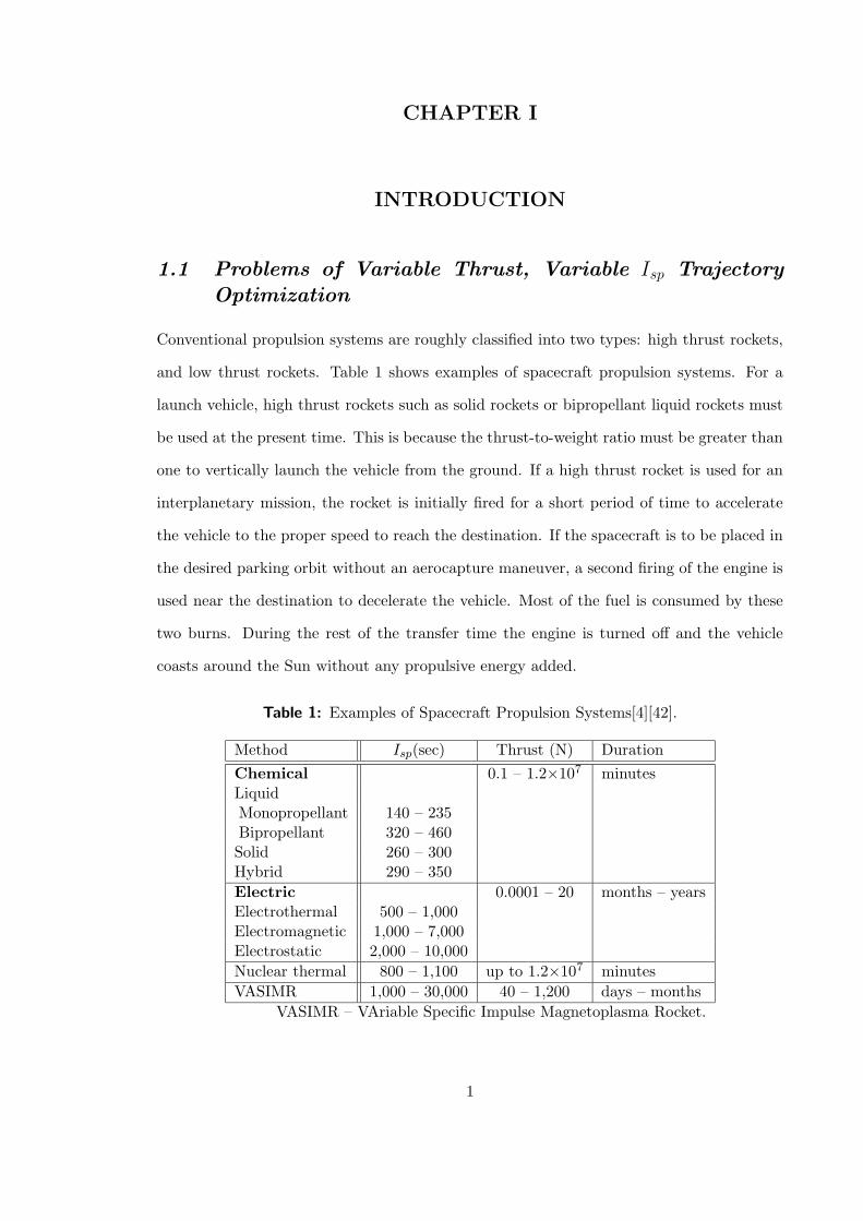
Conventional propulsion systems are roughly classified into two types: high thrust rockets,
and low thrust rockets. Table 1 shows examples of spacecraft propulsion systems. For a
launch vehicle, high thrust rockets such as solid rockets or bipropellant liquid rockets must
be used at the present time. This is because the thrust-to-weight ratio must be greater than
one to vertically launch the vehicle from the ground. If a high thrust rocket is used for an
interplanetary mission, the rocket is initially fired for a short period of time to accelerate
the vehicle to the proper speed to reach the destination. If the spacecraft is to be placed in
the desired parking orbit without an aerocapture maneuver, a second firing of the engine is
used near the destination to decelerate the vehicle. Most of the fuel is consumed by these
two burns. During the rest of the transfer time the engine is turned off and the vehicle
coasts around the Sun without any propulsive energy added.
Table 1: Examples of Spacecraft Propulsion Systems[4][42].
Method Isp(sec) Thrust (N) Duration
Chemical 0.1 – 1.2×10⁷ minutesLiquidMonopropellant 140 – 235Bipropellant 320 – 460Solid 260 – 300Hybrid 290 – 350
Electric 0.0001 – 20 months – yearsElectrothermal 500 – 1,000Electromagnetic 1,000 – 7,000Electrostatic 2,000 – 10,000
Nuclear thermal 800 – 1,100 up to 1.2×10⁷ minutes
VASIMR 1,000 – 30,000 40 – 1,200 days – months
VASIMR – VAriable Specific Impulse Magnetoplasma Rocket.
1
On the other hand, low thrust rockets cannot be used for a launch vehicle because the
thrust-to-weight ratio of the engine alone is less than one. Low thrust rockets do provide
an advantage for interplanetary missions. Low thrust engines typically have higher specific
impulse than higher thrust engines. This higher specific impulse results in less fuel being
consumed when compared to high thrust rockets. Due to the low thrust level, trip times
are typically longer for low thrust rockets when compared to the high thrust engines. This
is especially true if the spacecraft has to leave the gravity well of the Earth or if it has to
conduct an orbital insertion at the destination planet using its engines.
The comparison between low thrust systems and high thrust systems can be thought
of in the same way as the comparison between a car driving in low gear and a car driving
in high gear. A car starting from rest or climbing up a hill requires high thrust, and a
driver chooses low gear to exert high thrust at the expense of high fuel consumption. In
contrast, a car cruising on a highway needs high fuel efficiency rather than high thrust, so
a car cruising with high speed uses its top gear to save fuel.
A conventional propulsion system cannot modulate its specific impulse. So, depending
on the purpose of the mission, a mission designer must select the rocket type.
The concept of modulating thrust and specific impulse has been theoretically evaluated
since the early 1950’s[9][25]. Currently there are several projects ongoing worldwide relevant
to rocket engines that can modulate their thrust and Isp. This research includes mechanical
tests at ground facilities as well as trajectory simulations with computers. However, a ques-
tion emerges: “What are the advantages of having a propulsion system that can modulate
its specific impulse depending on the operational condition?”
The study of trajectory optimization problems is very important for space development.
If a trajectory can be optimized by either minimizing fuel consumption or finding the
best launch opportunity that minimizes time from Earth to another planetary body, that
trajectory will save operational costs as well as increase the probability of success of a
mission.
For high thrust engines, the interplanetary trajectory is nearly a conic section that is
2
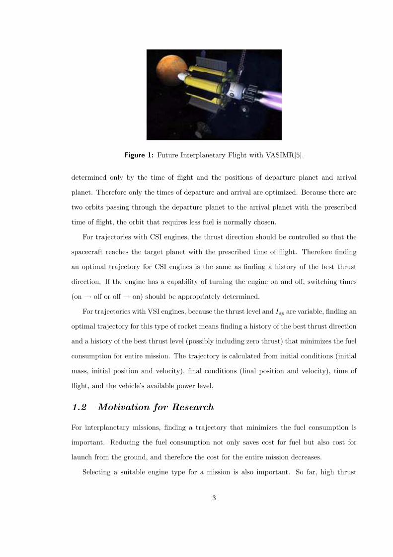
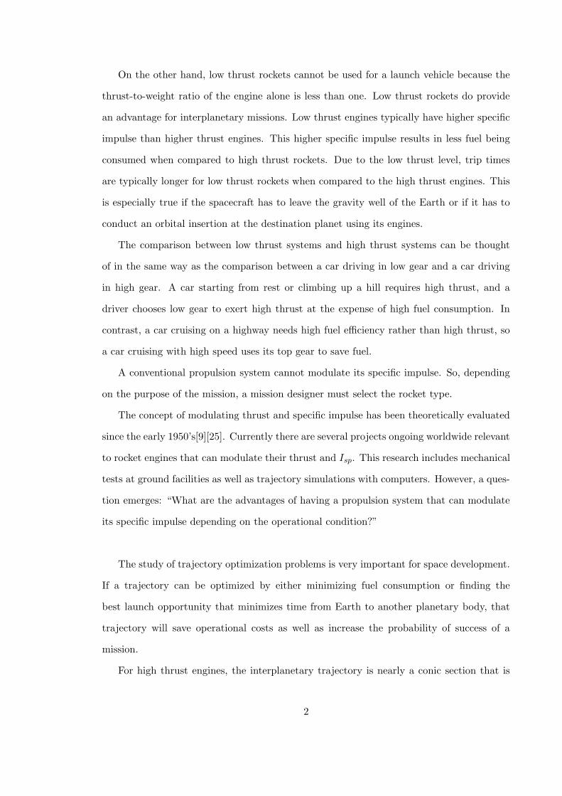
Figure 1: Future Interplanetary Flight with VASIMR[5].
determined only by the time of flight and the positions of departure planet and arrival
planet. Therefore only the times of departure and arrival are optimized. Because there are
two orbits passing through the departure planet to the arrival planet with the prescribed
time of flight, the orbit that requires less fuel is normally chosen.
For trajectories with CSI engines, the thrust direction should be controlled so that the
spacecraft reaches the target planet with the prescribed time of flight. Therefore finding
an optimal trajectory for CSI engines is the same as finding a history of the best thrust
direction. If the engine has a capability of turning the engine on and off, switching times
(on → off or off → on) should be appropriately determined.
For trajectories with VSI engines, because the thrust level and Isp are variable, finding an
optimal trajectory for this type of rocket means finding a history of the best thrust direction
and a history of the best thrust level (possibly including zero thrust) that minimizes the fuel
consumption for entire mission. The trajectory is calculated from initial conditions (initial
mass, initial position and velocity), final conditions (final position and velocity), time of
flight, and the vehicle’s available power level.
1.2 Motivation for Research
For interplanetary missions, finding a trajectory that minimizes the fuel consumption is
important. Reducing the fuel consumption not only saves cost for fuel but also cost for
launch from the ground, and therefore the cost for the entire mission decreases.
Selecting a suitable engine type for a mission is also important. So far, high thrust
3
Figure 2: Transfer Trajectory from Earth to Mars with Thrust Direction.
engines and constant Isp low thrust engines have been used for interplanetary missions. If a
variable Isp engine, which is under development, could be used for a mission, it may reduce
the mission cost. Analyzing trajectories with variable Isp engines and comparing them to
trajectories with constant Isp engines or high thrust engines should help in selecting the
engine type.
There have been several numerical research efforts for variable thrust, variable Isp (vari-
able specific impulse, or VSI), limited-power trajectory optimization problems [25][49][20]
[69][61][72]. Both indirect methods and direct methods have been used to evaluate this
problem. Most of the research efforts assume a human mission to Mars, and all of these
results conclude that VSI engines are superior to constant thrust, constant Isp (or CSI)
engines. That means VSI engines require less amount of propellant than CSI engines for a
mission.
This research started with the following questions:
• Does a VSI engine always require less fuel than a CSI engine or a high thrust engine
for any mission to any planet with any time of flight?
– If the answer is yes, is it possible to find a qualitative relationship between fuel
consumption and other parameters such as power level, time of flight, or semi-
major axis of the transfer orbit?
4
– If the answer is no, in what situations are CSI or high thrust better than VSI?
• If a planetary swing-by is used for a VSI trajectory, how much fuel can be saved
relative to the non swing-by case? Is the fuel saving of the VSI swing-by trajectory
better than that of a CSI swing-by trajectory or a high thrust swing-by trajectory?
To answer the above questions, a study of a variable thrust, variable Isp rocket engine,
particularly focusing on the optimization of interplanetary trajectories with this type of
rocket engine, is conducted in this research. A number of interplanetary trajectories with
different combinations of departure date, time of flight, and target planet are simulated
numerically and the fuel consumption for VSI, CSI, and high thrust engines are compared.
1.3 Research Goals and Objectives
The primary goal of this research is to demonstrate the advantages and disadvantages of
VSI engines over conventional engines such as CSI engines and high thrust engines that are
currently used for interplanetary missions. If the merits and demerits of using a VSI engine
over a CSI engine and a high thrust engine are parameterized, this data can be used to
determine the engine type for a particular mission. Therefore, the goal of this research is
to establish a generalized rule that:
1. Qualitatively states the advantages and disadvantages of a VSI engine.
2. Quantitatively determines the fuel savings by using a VSI engine over a CSI or a high
thrust engine.
For example, goal 1 may be written as, “to travel from Earth to Mars, VSI is always
better than other types of engines, but as the trip time increases the merit of using a VSI
engine gradually decreases.” Similarly, goal 2 may be written as, “going from Earth to
Jupiter in 3 years with a VSI engine saves about 20% of the total fuel over a CSI engine
and 33% over a high thrust engine.”
5
To support the goal described above, numerical analyses should be conducted. As far as
the author knows, there are currently no programs available that can calculate interplan-
etary trajectories with all of VSI, CSI, and high thrust engines. Therefore, an additional
goal is to create an interplanetary trajectory optimization program that can calculate the
trajectories to conduct this research.
The program should have the capability of calculating transfer trajectories from one
planet to another, and it should be used for any type of engine including VSI, CSI, and
high thrust. The program also should be able to calculate swing-by trajectories with those
same types of engines. The program should be robust, accurate, and fast.
1.4 Approach
To achieve the above research objectives, several steps were taken in this research.
At first, to become familiar with interplanetary optimization problems, a literature
review was conducted. This work included finding and studying a proper method to solve
this kind of problem, understanding orbital mechanics and methods of solving optimization
problems, and addressing the contribution of this research to the field of interplanetary
trajectory optimization problems.
Next, proof-of-concept study was conducted that was designed to be simple, yet still
representative of the problems. A simple two-dimensional trajectory was used to compare
fuel consumption of VSI, CSI, and high thrust engines by integrating equations of motion.
Then an interplanetary trajectory optimization software application was created using
a method learned during the literature review. The application was developed to be easy
to use, run quickly, and produce accurate results.
Using this application, a preliminary study was conducted to confirm the implementation
of the application. Assuming that the orbits of planets around the Sun are circular and
coplanar, two-dimensional trajectories from Earth to other planets were calculated. With
this research, a large database was obtained regarding fuel requirements. A rule of thumb for
the relationship between fuel requirements and the distance from Earth to target planets as
well as the relationship between fuel requirements and time of flight for each type of engine
6
was established.
Finally, “real world” examples were considered to check if the relationships obtained in
the previous step can be applied to the actual three-dimensional interplanetary trajectories.
Planet positions and velocities are given as functions of time that are obtained from actual
observations. Using the position and velocity data for planets, simulations for transfer
trajectories were conducted.
1.5 Organization of the Thesis
This thesis is organized into nine chapters and four appendices:
• Chapter 2 is an overview of trajectory optimization problems. Examples of general
trajectory optimization problems are presented. Then several research efforts for low
thrust trajectories that have been done by other researchers are introduced from the
literature review.
General optimization problems are also described in this chapter. At first, several
optimization methods are introduced. The method of calculus of variations that is
then applied to different types of optimization problems is presented.
• Chapter 3 briefly describes an engine that is capable of modulating thrust and specific
impulse. In this chapter, as an example of a VSI engine, the mechanism of the
VASIMR engine that is currently under development at NASA Johnson Space Center
is presented. Then this chapter provides a mathematical way of finding the best power
level to be operated throughout the mission.
• Chapter 4 presents the preliminary, proof-of-concept study with simple trajectories.
Using 2D simple spiral trajectories between two attracting bodies, the fuel consump-
tion of high thrust, low thrust with constant Isp, and low thrust with variable Isp are
compared.
• Chapter 5 describes general interplanetary trajectory optimization problems. The
assumptions made to conduct this research are first defined, and then the required
equations of motion to solve the optimization problems are determined.
7
• Chapter 6 explains the development of the software application SAMURAI in detail.
Capabilities of this application, C++ classes and schemes, and example inputs and
outputs are shown. A brief explanation of VRML that displays the trajectory on the
web browser is also described.
• Chapter 7 shows the preliminary results from SAMURAI. Two-dimensional transfer
trajectories between planets are calculated. Planets are assumed to be orbiting around
the Sun with zero eccentricity and zero inclination. The results of this computation
are presented.
• Chapter 8 shows the “real world” numerical examples. Using three-dimensional actual
ephemeris data of planets, transfer trajectories from Earth to other planets with and
without swing-bys are computed. Then a summary and the knowledge obtained from
this data are presented.
• Chapter 9 closes the thesis with conclusions and recommendations for future work.
• There are four appendices: Appendix A shows the results for the preliminary study
obtained in Chapter 7, Appendix B provides the additional equations used in the
application.
Chapter C introduces all the programming techniques required to solve the problems
proposed in this research. The examples of techniques introduced in this section are
optimal control programming, line search, Powell’s method, and penalty functions.
Appendix D is the users’ manual for the application SAMURAI.
8
CHAPTER II
A BRIEF DESCRIPTION OF LOW THRUST
TRAJECTORY OPTIMIZATION
2.1 Trajectory Optimization in General
Trajectory optimization can be defined as finding the “best” path from an initial condition
to some final condition based on a certain performance index [79]. Finding the best path in
this case could be rephrased as finding the best thrust history (direction and magnitude)
for a given mission. The performance index depends on the characteristics of the problem.
For a minimum-fuel, fixed-time, and fixed-initial mass problem, we would like to maximize
the final mass of the space vehicle at the end of transfer time. The objective function to be
minimized is the negative of the final mass of the vehicle. Whereas, for a minimum-time
problem, transfer time from one point to another will be of interest, so the performance
index is the transfer time. combination of a minimum-time problem and a minimum-fuel
problem. If the operating cost is a function of the transfer time and they are proportional
to each other, we would like to minimize the transfer time to minimize the cost. But to
achieve the minimum transfer time we need large amount of fuel. Therefore, for example, if
we would like to minimize the cost, the following problem should be solved: “Find the best
launch opportunity for a transfer orbit from Earth to Mars that minimizes the cost. This
cost is the combination of fuel consumption and transfer time if we leave Earth between year
2005 and 2020.” For this type of problem, a grid search may be necessary at the beginning
of the analysis with the launch date and time of flight as parameters. The results gained
from the grid search will allow a more precise optimization to be performed.
2.2 Solution Methods for Optimization Problems
Solution methods for trajectory optimization problems are typically identified as either
direct methods or indirect methods. In this section the characteristics of these methods are
9
presented.
Direct methods discretize the optimization problem through events and phases, and
the subsequent problem is solved using nonlinear programming techniques[55]. These tech-
niques include shooting, multiple shooting, and transcription or collocation methods. In
the shooting method, the control history is discretized as a polynomial, with the trajectory
variables as functions of the integrated equations of motion. In the collocation method, the
trajectory is discretized over an entire trajectory as a set of polynomials for both state vari-
ables and control variables[55]. Solutions obtained with these direct methods are generally
considered sub-optimal due to the discretization of either the state or controls, or both[69].
Indirect methods use calculus of variations techniques to characterize the optimization
problem as a two-point boundary value problem. The optimal control scheme is an indirect
method. The optimal control uses a first variation technique to determine necessary condi-
tions for an optimum, and second variation techniques are used to determine whether the
point is the minimum, the maximum, or a saddle point[17]. This method involves applying
calculus of variations principles and solving the corresponding two point boundary value
problem[51]. Initial estimates of the Lagrange multipliers must be provided, but since they
do not have physical meanings, guessing the initial values of the Lagrange multiplier is
difficult and may lead to problems with convergence.
There also exist hybrid methods that numerically integrate the Euler-Lagrange equations
(and control the spacecraft based on the primer vector). These methods solve a nonlinear
programming problem where the Lagrange multipliers of the indirect method and the rel-
evant mission parameters form part of the parameter vector while extremizing a general
scalar cost function[69].
Each of the above methods have pros and cons: indirect methods are difficult to formu-
late, whereas with direct methods, mathematical suboptimal solutions are obtained. In this
research, an indirect method is selected since they calculate an optimal solution rather than a
suboptimal solution. The equations of motion used in this research are not very complicated
and can be implemented into the application without difficulties. Also, there are several
10
excellent literature available for programming with indirect methods[17][49][69][41][57].
2.3 Indirect Methods – Calculus of Variations
The calculus of variations is concerned with the problem of minimizing or maximizing
functionals, a functional being a quantity whose value depends upon the sets of values
taken by certain associated functions over domains of their variables for which they are
defined[54]. In this section, some methods to solve different types of optimization problems
are described.
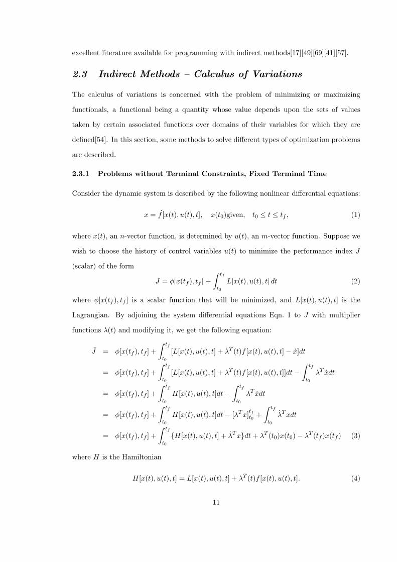
2.3.1 Problems without Terminal Constraints, Fixed Terminal Time
Consider the dynamic system is described by the following nonlinear differential equations:
x = f [x(t), u(t), t], x(t0)given, t0 ≤ t ≤ tf , (1)
where x(t), an n-vector function, is determined by u(t), an m-vector function. Suppose we
wish to choose the history of control variables u(t) to minimize the performance index J
(scalar) of the form
J = φ[x(tf ), tf ] +
∫ tf
t0
L[x(t), u(t), t] dt (2)
where φ[x(tf ), tf ] is a scalar function that will be minimized, and L[x(t), u(t), t] is the
Lagrangian. By adjoining the system differential equations Eqn. 1 to J with multiplier
functions λ(t) and modifying it, we get the following equation:
J = φ[x(tf ), tf ] +
∫ tf
t0
[L[x(t), u(t), t] + λT (t)f [x(t), u(t), t] − x]dt
= φ[x(tf ), tf ] +
∫ tf
t0
[L[x(t), u(t), t] + λT (t)f [x(t), u(t), t]]dt−∫ tf
t0
λT xdt
= φ[x(tf ), tf ] +
∫ tf
t0
H[x(t), u(t), t]dt−∫ tf
t0
λT xdt
= φ[x(tf ), tf ] +
∫ tf
t0
H[x(t), u(t), t]dt− [λTx]tft0
+
∫ tf
t0
λTxdt
= φ[x(tf ), tf ] +
∫ tf
t0
H[x(t), u(t), t] + λTxdt+ λT (t0)x(t0) − λT (tf )x(tf ) (3)
where H is the Hamiltonian
H[x(t), u(t), t] = L[x(t), u(t), t] + λT (t)f [x(t), u(t), t]. (4)
11
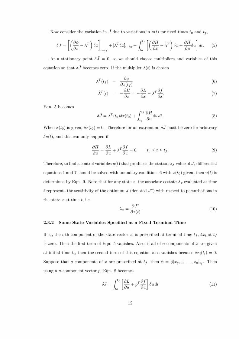
Now consider the variation in J due to variations in u(t) for fixed times t0 and tf ,
δJ =
[(
∂φ
∂x− λT
)
δx
]
t=tf
+ [λT δx]t=t0 +
∫ tf
t0
[(
∂H
∂x+ λT
)
δx+∂H
∂uδu
]
dt. (5)
At a stationary point δJ = 0, so we should choose multipliers and variables of this
equation so that δJ becomes zero. If the multiplier λ(t) is chosen
λT (tf ) =∂φ
∂x(tf )(6)
λT (t) = −∂H∂x
= −∂L∂x
− λT∂f
∂x, (7)
Eqn. 5 becomes
δJ = λT (t0)δx(t0) +
∫ tf
t0
∂H
∂uδu dt. (8)
When x(t0) is given, δx(t0) = 0. Therefore for an extremum, δJ must be zero for arbitrary
δu(t), and this can only happen if
∂H
∂u=∂L
∂u+ λT
∂f
∂u= 0, t0 ≤ t ≤ tf . (9)
Therefore, to find a control variables u(t) that produces the stationary value of J , differential
equations 1 and 7 should be solved with boundary conditions 6 with x(t0) given, then u(t) is
determined by Eqn. 9. Note that for any state x, the associate costate λx evaluated at time
t represents the sensitivity of the optimum J (denoted J ∗) with respect to perturbations in
the state x at time t, i.e.
λx =∂J∗
∂x(t)(10)
2.3.2 Some State Variables Specified at a Fixed Terminal Time
If xi, the i-th component of the state vector x, is prescribed at terminal time tf , δxi at tf
is zero. Then the first term of Eqn. 5 vanishes. Also, if all of n components of x are given
at initial time ti, then the second term of this equation also vanishes because δxi(ti) = 0.
Suppose that q components of x are prescribed at tf , then φ = φ[xq+1, · · · , xn]tf . Then
using a n-component vector p, Eqn. 8 becomes
δJ =
∫ tf
t0
[
∂L
∂u+ pT
∂f
∂u
]
δu dt (11)
12
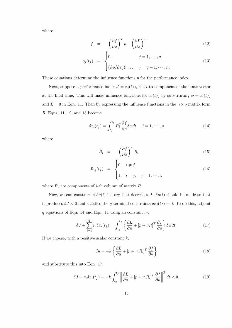
where
p = −(
∂f
∂x
)T
p−(
∂L
∂x
)T
(12)
pj(tf ) =
0, j = 1, · · · , q
(∂φ/∂xj)|t=tf , j = q + 1, · · · , n.(13)
These equations determine the influence functions p for the performance index.
Next, suppose a performance index J = xi(tf ), the i-th component of the state vector
at the final time. This will make influence functions for xi(tf ) by substituting φ = xi(tf )
and L = 0 in Eqn. 11. Then by expressing the influence functions in the n× q matrix form
R, Eqns. 11, 12, and 13 become
δxi(tf ) =
∫ tf
t0
RTi∂f
∂uδu dt, i = 1, · · · , q (14)
where
Ri = −(
∂f
∂x
)T
Ri (15)
Rij(tf ) =
0, i 6= j
1, i = j, j = 1, · · ·n,(16)
where Ri are components of i-th column of matrix R.
Now, we can construct a δu(t) history that decreases J . δu(t) should be made so that
it produces δJ < 0 and satisfies the q terminal constraints δxi(tf ) = 0. To do this, adjoint
q equations of Eqn. 14 and Eqn. 11 using an constant νi.
δJ +
q∑
i=1
νiδxi(tf ) =
∫ tf
t0
∂L
∂u+ [p+ νR]T
∂f
∂u
δu dt. (17)
If we choose, with a positive scalar constant k,
δu = −k
∂L
∂u+ [p+ νiRi]
T ∂f
∂u
(18)
and substitute this into Eqn. 17,
δJ + νiδxi(tf ) = −k∫ tf
t0
∥
∥
∥
∥
∂L
∂u+ [p+ νiRi]
T ∂f
∂u
∥
∥
∥
∥
2
dt < 0, (19)
13
which is negative unless the integrand vanishes. Therefore, if we can determine nui so that
it satisfies the terminal constraints(δxi(tf ) = 0), the performance index decreases with δu
of Eqn. 18. Substituting Eqn. 18 into Eqn. 14,
0 = δx(tf ) = −k∫ tf
t0
RT∂f
∂u
[
(
∂f
∂u
)T
[p+ νR] +
(
∂L
∂u
)T]
dt (20)
0 =
∫ tf
t0
RT∂f
∂u
[
(
∂f
∂u
)T
p+
(
∂L
∂u
)T]
dt+ ν
∫ tf
t0
RT(
∂f
∂u
)(
∂f
∂u
)T
Rdt, (21)
from which the appropriate choice of the νi’s is
ν = −Q−1g, (22)
where Q is a (q × q) matrix and g is a q-component vector:
Qij =
∫ tf
t0
RT(
∂f
∂u
)(
∂f
∂u
)T
Rdt, i, j = 1, · · · , q, (23)
gi =
∫ tf
t0
RT∂f
∂u
[
(
∂f
∂u
)T
p+
(
∂L
∂u
)T]
dt, i = 1, · · · , q. (24)
Thus, a δu(t) history that minimizes the performance index has been constructed.
If the terminal state is prescribed as a form of functions
ψ[x(tf ), tf ] = 0 q equations, (25)
the performance index can be written with a multiplier vector ν (a q vector) as follows.
J = φ[x(tf ), tf ] + νTψ[x(tf ), tf ] +
∫ tf
t0
L[x(t), u(t), t] dt. (26)
If we define a scalar function Φ = φ+ νTψ, the development above can be applied without
change. Then necessary conditions for J to have a stationary value are
x = f(x(t), u(t), t) (27)
λ = −∂f∂x
T
λ− ∂L
∂x
T
(28)
∂H
∂u
T
=∂f
∂u
T
λ+∂L
∂u
T
= 0 (29)
λT (tf ) =
(
∂φ
∂x+ νT
∂ψ
∂x
)
t=tf
(30)
ψ[x(tf ), tf ] = 0 (31)
x(t0) given. (32)
14
2.3.3 Inequality Constraints on the Control Variables
Suppose that we have an inequality constraint on the system:
C(u(t), t) ≤ 0. (33)
where u(t) is the m-component control vector, m ≥ 2, and C is a scalar function. For
example, when we would like to limit the Isp level less than or equal to 30,000m/s, C is
expressed as C = Isp − 30, 000 ≤ 0.
If we define the Hamiltonian with a Lagrange multiplier µ(t)
H = λT f + L+ µTC, (34)
the necessary condition on H is
Hu = λT fu + Lu + µTCu = 0 (35)
and µ
≥ 0, C = 0,
= 0, C < 0.
(36)
The positivity of the multiplier µ when C = 0 is interpreted as the requirement that the
gradient of original Hamiltonian (λT fu + Lu) be such that improvement can only come by
violating the constraints.
The differential equations for costate vectors are
λT (t) = −∂H∂x
= −∂L∂x
− λT∂f
∂x− µTCx = −∂L
∂x− λT
∂f
∂x. (37)
Therefore to calculate costate vectors we can use Eqn. 7 because C is not a function
of x. Boundary conditions should be chosen so that the initial and terminal constraints for
state variables are satisfied.
2.3.4 Bang-off-bang Control
This type of control is applied to the fixed-time, minimum-fuel problem with constrained
input magnitude. For example, a CSI rocket that can turn its engine on/off as needed would
obey this control law.
15
Consider the problem with the following linear system[57].
x = Ax+Bu (38)
Assume that the fuel used in each component of the input is proportional to the mag-
nitude of that component. Then the cost function to be minimized is
J(t0) =
∫ tf
ti
m∑
i=1
ci|ui(t)|dt, (39)
where ci is a component of a m vector C = [c1 c2 · · · cm]T and ui(t) is a component of a m
vector |u(t)| = [|u1| |u2| · · · |um|]T .
Suppose that the control is constrained as
|u(t)| ≤ 1 ti ≤ t ≤ tf . (40)
The Hamiltonian is
H = CT |u| + λT (Ax+Bu) (41)
and according to the Pontryagin’s minimum principle, the optimal control must satisfy
CT |u∗| + (λ∗)T (Ax∗ +Bu∗) ≤ CT |u| + (λ∗)T (Ax∗ +Bu) (42)
for all admissible u(t). (∗) denotes optimal quantities. This equation can be reduced to
CT |u∗| + (λ∗)TBu∗ ≤ CT |u| + (λ∗)TBu (43)
If we assume that all of the m components of the control variables are independent,
|u∗i | +(λ∗)T biu
∗
i
ci≤ |ui| +
(λ∗)T biuici
, (44)
where bi are the columns of B. Since
|ui| =
ui, ui ≥ 0
−ui, ui ≤ 0
(45)
we can write the quantity we are trying to minimize by selection of ui(t) as
qi(t) = |ui| +bTi λuici
=
(
1 + bTi λ/ci)
|ui|, ui ≥ 0
(
1 − bTi λ/ci)
|ui|, ui ≤ 0
(46)
16
q i u i =1 u i =-1
1
-1 1 0
b i T /c i u i =0
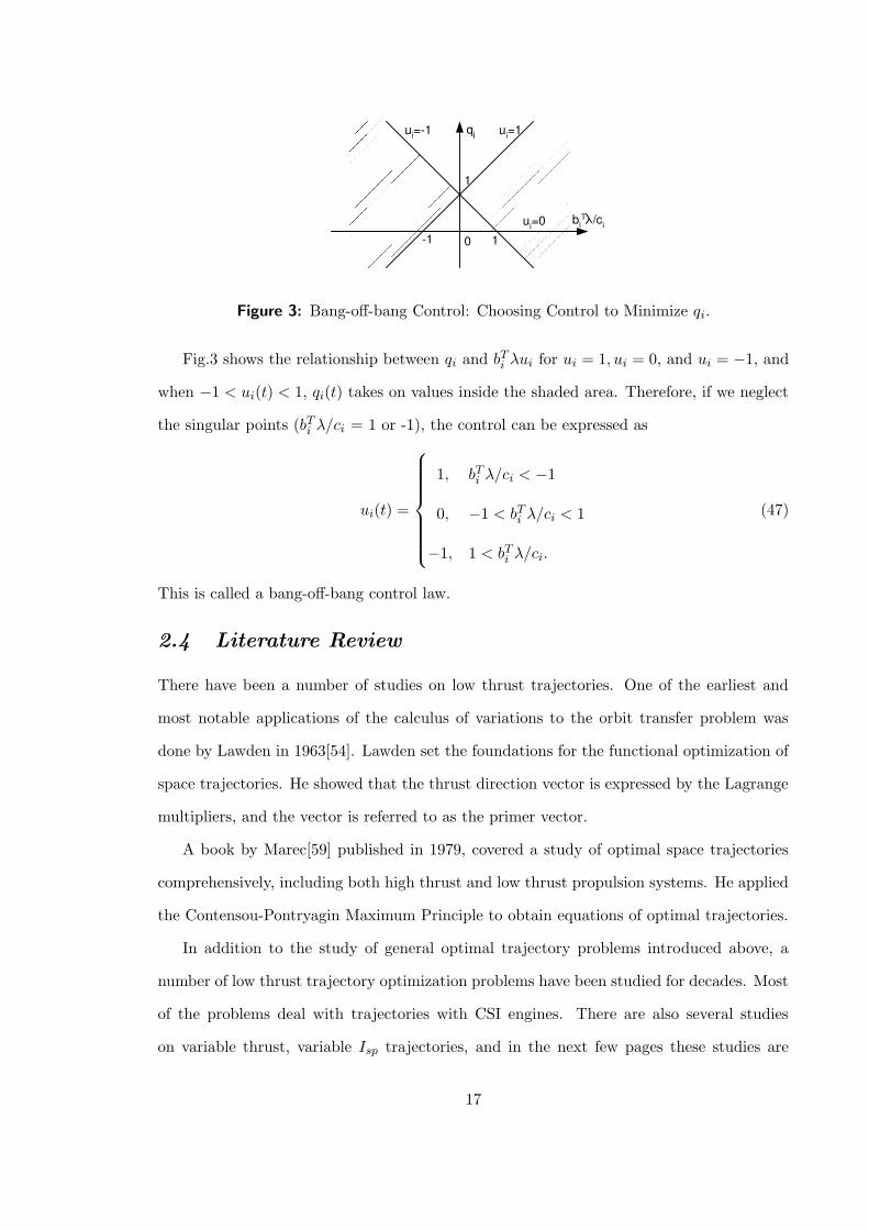
Figure 3: Bang-off-bang Control: Choosing Control to Minimize qi.
Fig.3 shows the relationship between qi and bTi λui for ui = 1, ui = 0, and ui = −1, and
when −1 < ui(t) < 1, qi(t) takes on values inside the shaded area. Therefore, if we neglect
the singular points (bTi λ/ci = 1 or -1), the control can be expressed as
ui(t) =
1, bTi λ/ci < −1
0, −1 < bTi λ/ci < 1
−1, 1 < bTi λ/ci.
(47)
This is called a bang-off-bang control law.
2.4 Literature Review
There have been a number of studies on low thrust trajectories. One of the earliest and
most notable applications of the calculus of variations to the orbit transfer problem was
done by Lawden in 1963[54]. Lawden set the foundations for the functional optimization of
space trajectories. He showed that the thrust direction vector is expressed by the Lagrange
multipliers, and the vector is referred to as the primer vector.
A book by Marec[59] published in 1979, covered a study of optimal space trajectories
comprehensively, including both high thrust and low thrust propulsion systems. He applied
the Contensou-Pontryagin Maximum Principle to obtain equations of optimal trajectories.
In addition to the study of general optimal trajectory problems introduced above, a
number of low thrust trajectory optimization problems have been studied for decades. Most
of the problems deal with trajectories with CSI engines. There are also several studies
on variable thrust, variable Isp trajectories, and in the next few pages these studies are
17
introduced.
In the paper published in 1995, Chang-Diaz, Hsu, Braden, Johnson, and Yang [25]
studied human-crewed fast trajectories with a VSI engine to and from Mars. Their study
does not include planetocentric phases at departure and arrival, but only heliocentric phase
is considered. In addition to completing a nominal round trip scenario (a 101-day outbound
trip, a 30-day stay, and a 104-day return), their work shows that a VSI engine has the
ability to abort a mission when something goes wrong during the outbound phase. Chang-
Diaz, an advocator of VASIMR(VAriable Specific Impulse Magnetoplasma Rocket), and
his colleagues have not only simulated the trajectory analysis but also have conducted a
number of hardware experiments with a VSI engine[65][74][43][66][30][44].
Kechichian(1995)[49] described the method of optimizing a VSI low thrust trajectory
from LEO to GEO using a set of non-singular equinoctial orbital elements. His paper
includes all the equations required to perform the calculus of variations to find the set of
control variables (Isp, pitch, and yaw) for a constant power, variable Isp trajectory. The
upper and lower bounds for the Isp are set to simulate the physical constraints of the engine.
This study is only for the orbit around the Earth and the equations cannot be used for the
escape trajectory as the equinoctial orbital elements are only valid for a trajectory with an
eccentricity of less than one.
Casalino, Colasurdo, and Pastrone(1999)[20] analyzed the optimal 2-dimensional helio-
centric trajectory with a VSI engine. Using the shooting method, they studied trajectories
with and without swing-bys to escape from the solar system. Their main concern was to
obtain the best history of thrust and pitch angle to maximize the specific energy of the
spacecraft at the end of calculation which does not have a planetary capture at the end.
The conclusion of this research was that a trajectory with swing-bys can get more escape
energy than a trajectory without swing-bys.
The research of VSI trajectories done by Nah and Vadali(2001)[61] includes the gravi-
tational effects of the Sun, the departure planet (Earth), and the arrival planet throughout
an entire trajectory. Mars is chosen as the arrival planet, and the actual ephemeris for
Earth and Mars is used. A shooting method was used to obtain the control variables that
18
maximize the final mass of the spacecraft at Mars arrival. The upper limit for Isp is set as
a constraint.
Seywald, Roithmayr, and Troutman(2003)[72] studied a circular-to-circular low thrust
orbit transfer with a prescribed transfer time. They solved the optimal control problem an-
alytically and studied the thrust history that minimizes the fuel consumption for a transfer
orbit between two circular orbits with prescribed time of flight. Their work concludes that,
if the thrust magnitude is always low enough such that it qualifies as “low thrust”, the op-
timal thrust magnitude is always proportional to the vehicle mass. They also investigated
how much fuel is saved if a VSI engine, instead of a CSI engine, is used, and concluded that
the percentage of fuel savings depends strongly on the boundary conditions such as flight
time and initial and final values of the semi-major axis.
The work done by Ranieri and Ocampo(2003)[69] is specialized for human missions to
Mars. Using the nonlinear programming boundary value solver, they studied a round trip
to Mars using VASIMR. This trajectory includes a heliocentric outbound trajectory from
Earth to Mars, a several month stay at Mars, then a heliocentric inbound trajectory from
Mars to Earth. Planetary bodies are assumed to be point masses (zero sphere of influence).
The objective is either to minimize the initial mass with a given final mass or to maximize
the final mass with a given initial mass for an unbounded Isp engine and a CSI engine. A
CSI engine can turn its power on and off, resulting in a bang-off-bang thrust profile. In
this paper, the fuel requirements for a round trip with VSI and a trajectory with CSI are
compared. The results show that the fuel consumption with VSI is more than the CSI for
the outbound trajectory, but it is less than CSI for the inbound trajectory. The result is
that VSI requires less fuel than CSI for an overall round trip.
Each of these papers gives interesting features of VSI engines. No paper compares VSI
engines with high thrust engines, and only two papers (by Seywald[72] and by Ranieri[69])
compare a VSI engine with a CSI engine. The paper by Ranieri studied Earth to Mars and
Mars to Earth trajectories, and the paper by Seywald studied circular-to-circular geocentric
transfer orbits. That means there still remains ambiguity of the advantages of a VSI engine
19
over a CSI engine in general. A swing-by trajectory was studied in Casalino’s paper[20],
but he does not include planetary capture at the end of the mission.
Therefore, it is still ambiguous if using the VSI engines is more beneficial than using
the CSI engines for any interplanetary missions. Also, the effects of planetary swing-bys for
transfer orbits between two planets are unknown.
Hence, research questions still remain: Is VSI always better than CSI or high thrust for
any trajectory? Or if we apply swing-bys and simulate a planetary capture at the end of
mission, what characteristics does the trajectory have?
20
CHAPTER III
EXHAUST-MODULATED PLASMA PROPULSION
SYSTEMS
This chapter contains a brief description of an engine that is capable of modulating thrust
and specific impulse at constant power.
There are several types of exhaust modulated engines under experiment such as VASIMR
(VAriable Specific Impulse Magnetoplasma Rocket), currently studied at the Advanced
Space Propulsion Laboratory at NASA’s Johnson Space Center in Houston (Fig. 4), or EICR
(Electron and Ion Cyclotron Resonance) Plasma Propulsion Systems at Kyushu University,
Japan[2].
Because these systems are similar, the mechanism of the VASIMR engine is presented
in this section.
3.1 Overview
The concept of exhaust modulation has been known theoretically since the early 1950’s[9][25],
but the technology to construct these systems had remained elusive until the late 1960’s.
The electric propulsion systems such as ion engines and the Hall thrusters accelerate ions
present in plasmas by applying electric fields externally or by charging axially. These ion
acceleration features, in turn, result in accelerated exhaust beams that must be neutralized
by electron sources located at the outlets before the exhaust streams leave the engine.
A MPD (Magnetoplasmadynamic thruster) plasma injector includes a cathode in contact
with the plasma. This cathode becomes eroded and the plasma becomes contaminated with
cathode material. This erosion and contamination limit the lifetime of the thruster and
degrade efficiency[23].
The design of the VASIMR avoids those limiting features as VASIMR has an electrode-
less design (a fact that enables the VASIMR to operate at much greater power densities).
21
DiffusionPumps
VacuumChamber Cryo
magnets
ICRH feedsPlasmaSource
Gas Injector
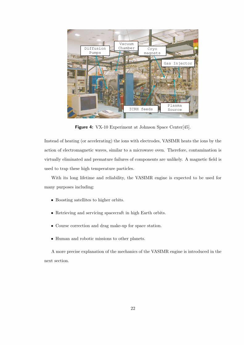
Figure 4: VX-10 Experiment at Johnson Space Center[45].
Instead of heating (or accelerating) the ions with electrodes, VASIMR heats the ions by the
action of electromagnetic waves, similar to a microwave oven. Therefore, contamination is
virtually eliminated and premature failures of components are unlikely. A magnetic field is
used to trap these high temperature particles.
With its long lifetime and reliability, the VASIMR engine is expected to be used for
many purposes including:
• Boosting satellites to higher orbits.
• Retrieving and servicing spacecraft in high Earth orbits.
• Course correction and drag make-up for space station.
• Human and robotic missions to other planets.
A more precise explanation of the mechanics of the VASIMR engine is introduced in the
next section.
22
3.2 Mechanism
Rocket thrust, T , is measured in Newtons (kg·m/s2) and is the product of the exhaust
velocity relative to the spacecraft, c(m/s), and the rate of propellant flow, m(kg/s).
T = −mc. (48)
The negative sign shows that the direction of the thrust is opposite to the direction of
the exhaust velocity. The same thrust is obtained by ejecting either more material at low
velocity or less material at high velocity. The latter saves fuel but generally entails high
exhaust temperatures.
The rocket performance is measured by its specific impulse, or Isp, which is the exhaust
velocity divided by the acceleration of gravity at sea level, g0(9.806m/s2), as
Isp =c
g0. (49)
The specific impulse is a rough measure of how fast the propellant is ejected out of the back
of the rocket. A rocket with a high specific impulse does not need as much fuel as a rocket
with a low specific impulse to achieve the same ∆V. Although thrust is directly proportional
to Isp (because T = −mc and c = g0Isp), the power needed to produce it is proportional
to the square of the Isp. Therefore the power required for a given thrust increases linearly
with Isp. These relationships can be expressed in the following equation:
PJ =T c
2= −1
2g0 Isp T = −1
2m g2
0 I2sp where PJ is the jet power. (50)
Chemical rockets obtain this power through the exothermic reaction of fuel and oxidizer.
In other propulsion systems, the power must be imparted to the exhaust by a propellant
heater or accelerator. Solar panels or nuclear reactors may be used to generate this power.
The greatest advantage of the VASIMR engine is that it can change its thrust level and
specific impulse at a constant power level by changing the amount and the velocity of the
exhaust ions. This is how VASIMR modulates its thrust and Isp.
VASIMR uses charged particles called plasma as a source of thrust. The temperature
of the plasma ranges from 10,000 K to more than 10 million K. At these temperatures, the
23
Magnetic Coils
ICRH Antennaheats gas
Helicon Antennaionizes gas
Quartz Tube
Gas Injector
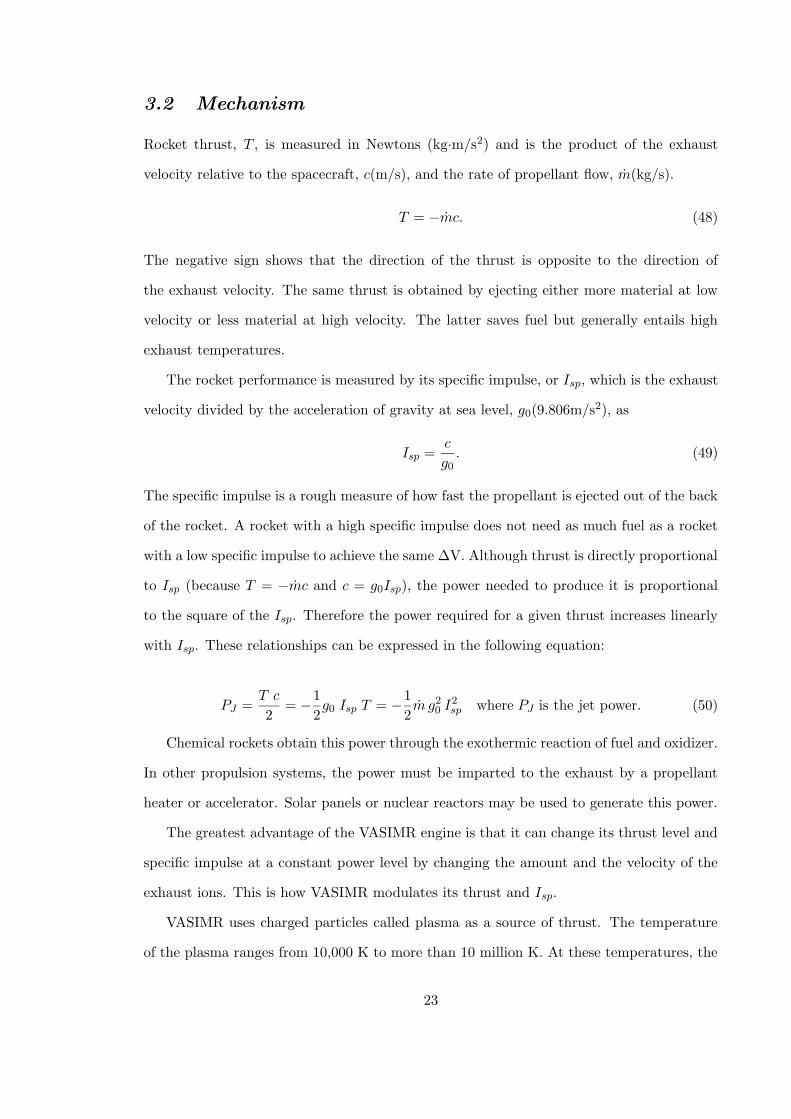
Figure 5: Synoptic View of the VASIMR Engine[22].
ions move at a velocity of 300,000 m/s. This is 60 times faster than the particles in the best
chemical rockets whose temperature is only about a few thousand K.
For a given jet power PJ , the relationship between thrust T and Isp is expressed as
PJ = 1
2T Isp g0. When the power is set constant, thrust and Isp are inversely related.
Increasing one always comes at the expense of the other.
As shown in Fig. 5[22], the VASIMR rocket system consists of three major magnetic cells
called “forward,” “central,” and “aft.” First, a neutral gas, typically hydrogen, is injected
from the injector to the forward cell and ionized by the helicon antenna[5].
Second, this charged gas is heated to reach the desired density in the engine’s central
cell. This heating process is done by the action of electromagnetic waves, which is similar
to what happens in a microwave oven. The plasma is trapped by the magnetic field that is
generated by the magnetic coils so that it can be heated to 10 million K.
Third, heated plasma enters the nozzle at the aft cell, where the plasma detaches from
the magnetic field and is exhausted to provide thrust.
VASIMR can change its thrust and Isp by changing the fraction of power sent to the
Helicon antenna vs. the ICRH antenna (See Fig. 6). The helicon antenna is used to ionize
24
Isp increases
Thrust increases
Power sent to ICRH antenna
Pmax = constant
Power sent to Helicon antenna
P1
P2
Pmax = P1 + P2
0
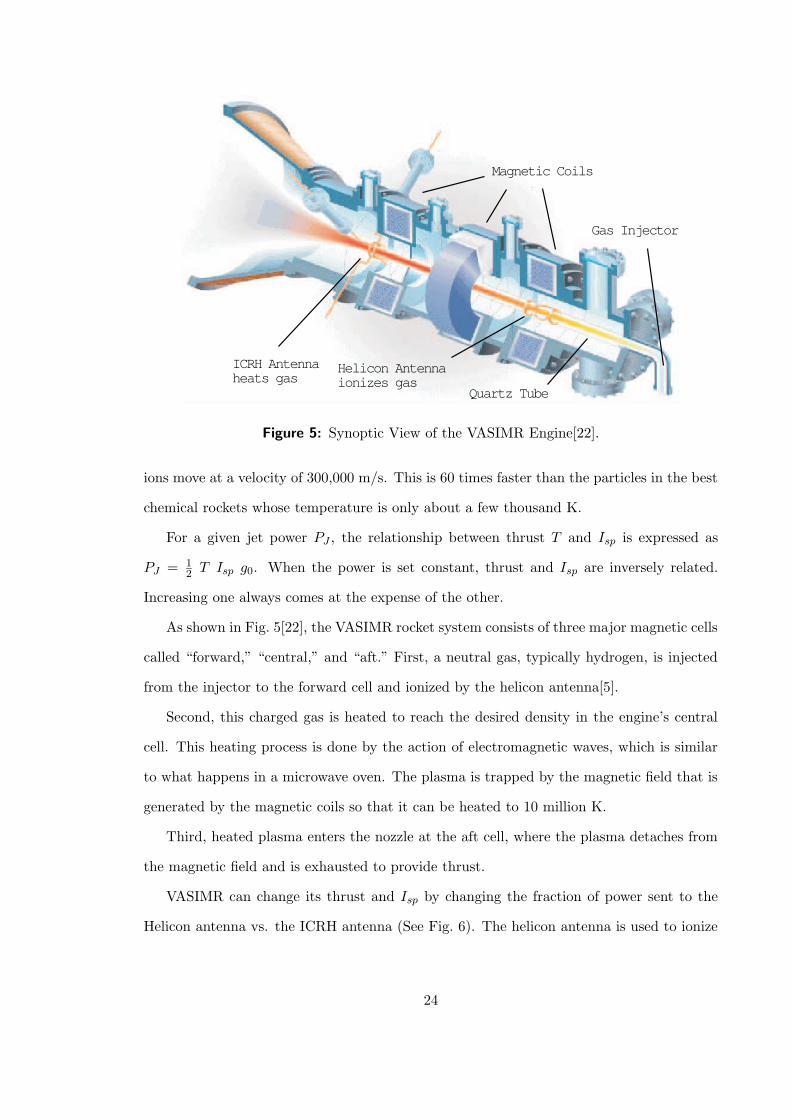
Figure 6: Power Partitioning and Relationship between Thrust and Isp.
gas injected from the gas injector. The ICRH (ion cyclotron resonance heating) antenna
heats the gas and accelerate the particle before these particles are exhausted to space. When
more power is sent to Helicon antenna, more gases are ionized, which means more ions are
ejected. But because the total system power level is constant, power sent to ICRH antenna
decreases, which means these ions exit with a lower velocity. These low speed, large quantity
of ions act as a source of a high thrust, low Isp engine. On the other hand, when less power
is sent to the Helicon antenna and more power is sent to the ICRH antenna, small amount
of gases are ionized and they are accelerated to a higher exit velocity. These high speed
ions act as a source of a low thrust, high Isp rocket engine.
In the absence of any constraints on the time required to perform a given orbital transfer,
it is always optimal to operate the engine at its highest possible specific impulse value.
However, if time is important, then it may be beneficial to trade some of the specific
impulse in return for high thrust[72].
As mentioned in Chap. 1, the choice of the combination of the thrust and Isp could be
considered in a similar way to an automobile transmission. Initially the spacecraft needs
high thrust so that it gets enough speed to begin the transfer. This is similar to a car
starting with low gear from rest. As the spacecraft’s speed increases, Isp is allowed to
gradually increase and therefore thrust decreases for higher fuel efficiency, just as a car
shifts up its gear as its speed increases.
25
3.3 Choosing the Power Level
In the last section, the operational power level is assumed to be maximum (therefore con-
stant). As explained so far, a VSI spacecraft needs high thrust near the departure planet
and target planet, but low fuel consumption is desirable for the rest of the path. VASIMR
has two options to lower fuel consumption: either by increasing Isp while the power is kept
constant or by decreasing the power level while Isp is kept constant.
In this section, fuel consumption at a power level other than the maximum is investigated
mathematically[49]. Then the reason the maximum power level should be always chosen to
achieve the least fuel consumption is presented.
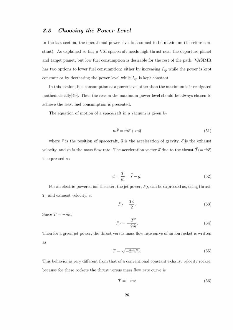
The equation of motion of a spacecraft in a vacuum is given by
m~r = m~c+m~g (51)
where ~r is the position of spacecraft, ~g is the acceleration of gravity, ~c is the exhaust
velocity, and m is the mass flow rate. The acceleration vector ~a due to the thrust ~T (= m~c)
is expressed as
~a =~T
m= ~r − ~g. (52)
For an electric-powered ion thruster, the jet power, PJ , can be expressed as, using thrust,
T , and exhaust velocity, c,
PJ =Tc
2. (53)
Since T = −mc,
PJ = − T 2
2m. (54)
Then for a given jet power, the thrust versus mass flow rate curve of an ion rocket is written
as
T =√
−2mPJ . (55)
This behavior is very different from that of a conventional constant exhaust velocity rocket,
because for these rockets the thrust versus mass flow rate curve is
T = −mc (56)
26
Tmax
T
-mO
T = -mc (linear)
c = g0Isp = constant
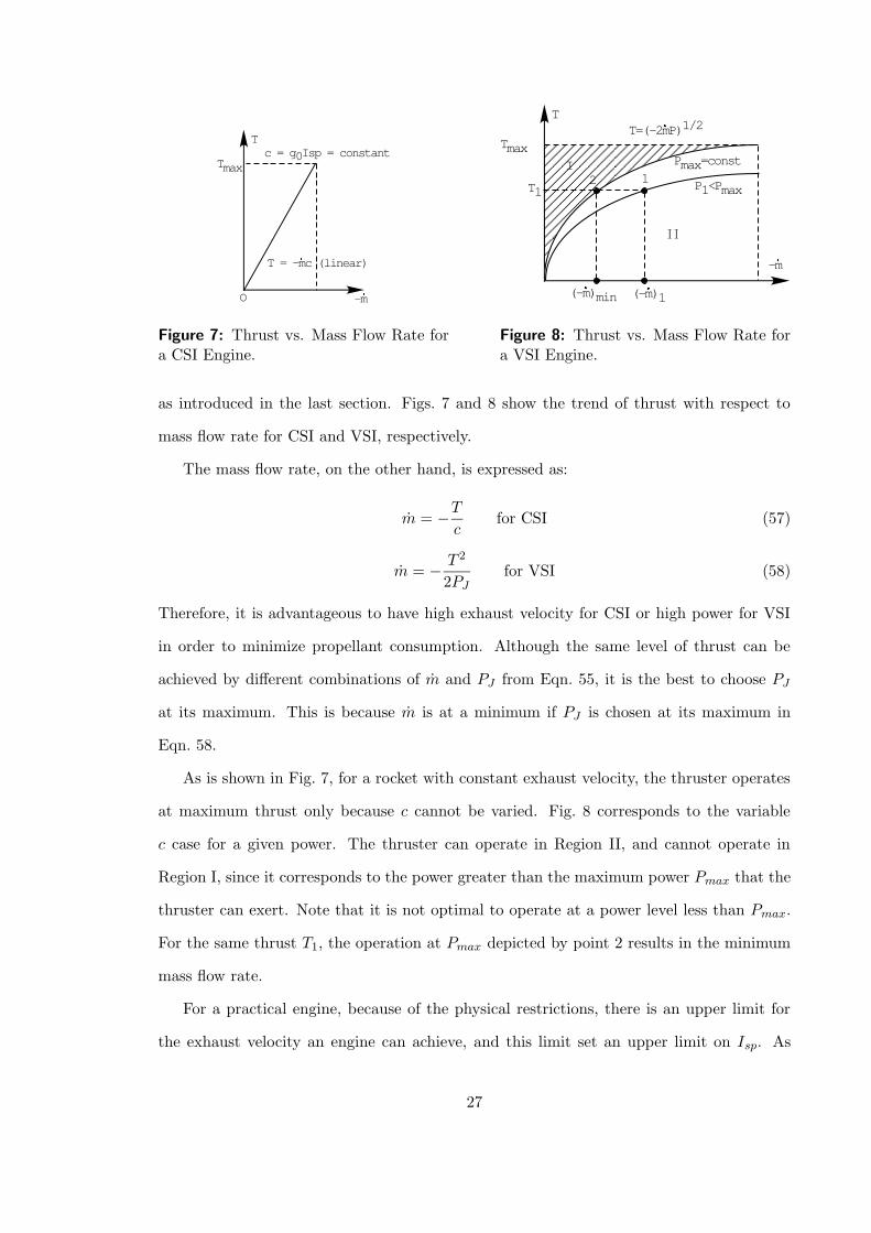
Figure 7: Thrust vs. Mass Flow Rate fora CSI Engine.
T1
Tmax
T
(-m)1(-m)min
-m
T=(-2mP)1/2
12
Pmax=const
P1<Pmax
I
Figure 8: Thrust vs. Mass Flow Rate fora VSI Engine.
as introduced in the last section. Figs. 7 and 8 show the trend of thrust with respect to
mass flow rate for CSI and VSI, respectively.
The mass flow rate, on the other hand, is expressed as:
m = −Tc
for CSI (57)
m = − T 2
2PJfor VSI (58)
Therefore, it is advantageous to have high exhaust velocity for CSI or high power for VSI
in order to minimize propellant consumption. Although the same level of thrust can be
achieved by different combinations of m and PJ from Eqn. 55, it is the best to choose PJ
at its maximum. This is because m is at a minimum if PJ is chosen at its maximum in
Eqn. 58.
As is shown in Fig. 7, for a rocket with constant exhaust velocity, the thruster operates
at maximum thrust only because c cannot be varied. Fig. 8 corresponds to the variable
c case for a given power. The thruster can operate in Region II, and cannot operate in
Region I, since it corresponds to the power greater than the maximum power Pmax that the
thruster can exert. Note that it is not optimal to operate at a power level less than Pmax.
For the same thrust T1, the operation at Pmax depicted by point 2 results in the minimum
mass flow rate.
For a practical engine, because of the physical restrictions, there is an upper limit for
the exhaust velocity an engine can achieve, and this limit set an upper limit on Isp. As
27
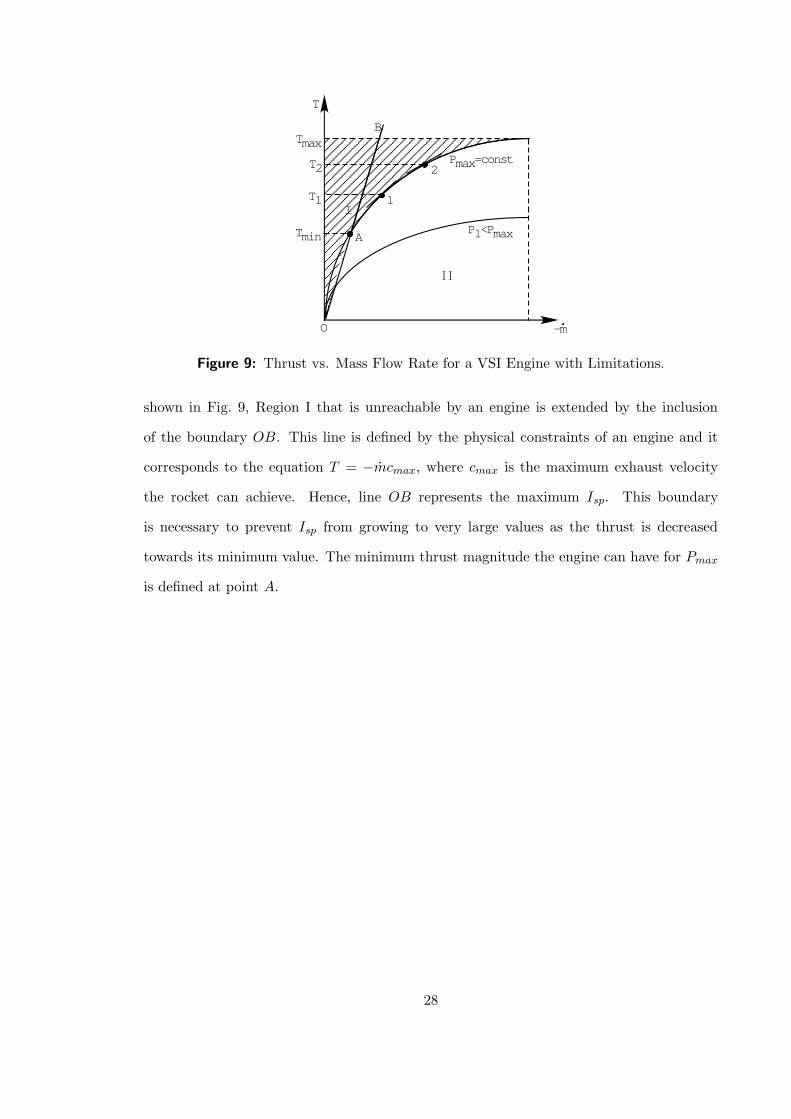
T1
Tmax
T
-m
1
2Pmax=const
P1<Pmax
I
Tmin
T2
O
A
B
Figure 9: Thrust vs. Mass Flow Rate for a VSI Engine with Limitations.
shown in Fig. 9, Region I that is unreachable by an engine is extended by the inclusion
of the boundary OB. This line is defined by the physical constraints of an engine and it
corresponds to the equation T = −mcmax, where cmax is the maximum exhaust velocity
the rocket can achieve. Hence, line OB represents the maximum Isp. This boundary
is necessary to prevent Isp from growing to very large values as the thrust is decreased
towards its minimum value. The minimum thrust magnitude the engine can have for Pmax
is defined at point A.
28
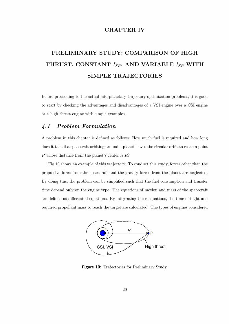
CHAPTER IV
PRELIMINARY STUDY: COMPARISON OF HIGH
THRUST, CONSTANT ISP , AND VARIABLE ISP WITH
SIMPLE TRAJECTORIES
Before proceeding to the actual interplanetary trajectory optimization problems, it is good
to start by checking the advantages and disadvantages of a VSI engine over a CSI engine
or a high thrust engine with simple examples.
4.1 Problem Formulation
A problem in this chapter is defined as follows: How much fuel is required and how long
does it take if a spacecraft orbiting around a planet leaves the circular orbit to reach a point
P whose distance from the planet’s center is R?
Fig 10 shows an example of this trajectory. To conduct this study, forces other than the
propulsive force from the spacecraft and the gravity forces from the planet are neglected.
By doing this, the problem can be simplified such that the fuel consumption and transfer
time depend only on the engine type. The equations of motion and mass of the spacecraft
are defined as differential equations. By integrating these equations, the time of flight and
required propellant mass to reach the target are calculated. The types of engines considered
R
CSI, VSI High thrust
P
Figure 10: Trajectories for Preliminary Study.
29
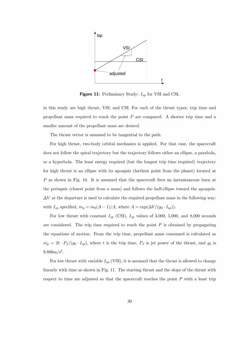
Isp
t
VSI
CSI
adjusted
Figure 11: Preliminary Study: Isp for VSI and CSI.
in this study are high thrust, VSI, and CSI. For each of the thrust types, trip time and
propellant mass required to reach the point P are compared. A shorter trip time and a
smaller amount of the propellant mass are desired.
The thrust vector is assumed to be tangential to the path.
For high thrust, two-body orbital mechanics is applied. For that case, the spacecraft
does not follow the spiral trajectory but the trajectory follows either an ellipse, a parabola,
or a hyperbola. The least energy required (but the longest trip time required) trajectory
for high thrust is an ellipse with its apoapsis (farthest point from the planet) located at
P as shown in Fig. 10. It is assumed that the spacecraft fires an instantaneous burn at
the periapsis (closest point from a mass) and follows the half-ellipse toward the apoapsis.
∆V at the departure is used to calculate the required propellant mass in the following way:
with Isp specified, mp = m0(A− 1)/A, where A = exp(∆V/(g0 · Isp)).
For low thrust with constant Isp (CSI), Isp values of 3,000, 5,000, and 8,000 seconds
are considered. The trip time required to reach the point P is obtained by propagating
the equations of motion. From the trip time, propellant mass consumed is calculated as
mp = 2t · PJ/(g0 · Isp), where t is the trip time, PJ is jet power of the thrust, and g0 is
9.806m/s2.
For low thrust with variable Isp (VSI), it is assumed that the thrust is allowed to change
linearly with time as shown in Fig. 11. The starting thrust and the slope of the thrust with
respect to time are adjusted so that the spacecraft reaches the point P with a least trip
30
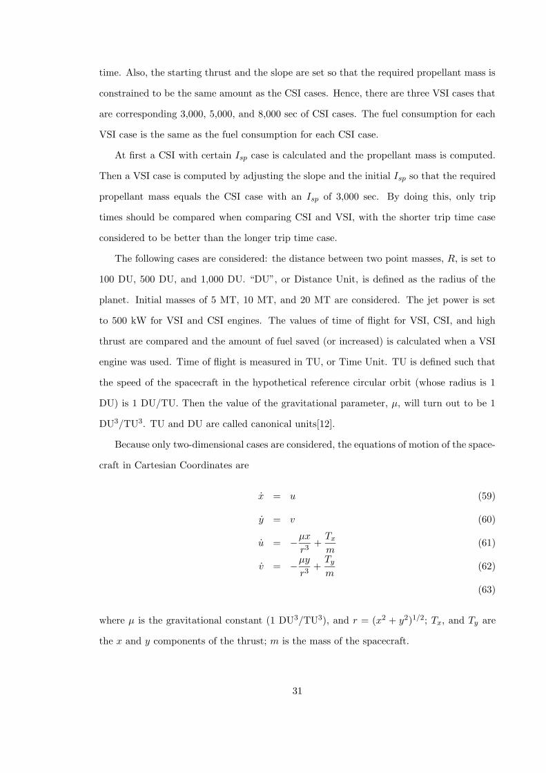
time. Also, the starting thrust and the slope are set so that the required propellant mass is
constrained to be the same amount as the CSI cases. Hence, there are three VSI cases that
are corresponding 3,000, 5,000, and 8,000 sec of CSI cases. The fuel consumption for each
VSI case is the same as the fuel consumption for each CSI case.
At first a CSI with certain Isp case is calculated and the propellant mass is computed.
Then a VSI case is computed by adjusting the slope and the initial Isp so that the required
propellant mass equals the CSI case with an Isp of 3,000 sec. By doing this, only trip
times should be compared when comparing CSI and VSI, with the shorter trip time case
considered to be better than the longer trip time case.
The following cases are considered: the distance between two point masses, R, is set to
100 DU, 500 DU, and 1,000 DU. “DU”, or Distance Unit, is defined as the radius of the
planet. Initial masses of 5 MT, 10 MT, and 20 MT are considered. The jet power is set
to 500 kW for VSI and CSI engines. The values of time of flight for VSI, CSI, and high
thrust are compared and the amount of fuel saved (or increased) is calculated when a VSI
engine was used. Time of flight is measured in TU, or Time Unit. TU is defined such that
the speed of the spacecraft in the hypothetical reference circular orbit (whose radius is 1
DU) is 1 DU/TU. Then the value of the gravitational parameter, µ, will turn out to be 1
DU3/TU3. TU and DU are called canonical units[12].
Because only two-dimensional cases are considered, the equations of motion of the space-
craft in Cartesian Coordinates are
x = u (59)
y = v (60)
u = −µxr3
+Txm
(61)
v = −µyr3
+Tym
(62)
(63)
where µ is the gravitational constant (1 DU3/TU3), and r = (x2 + y2)1/2; Tx, and Ty are
the x and y components of the thrust; m is the mass of the spacecraft.
31
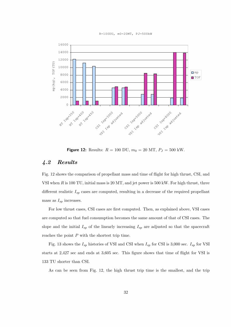
R=100DU, m0=20MT, PJ=500kW
0
2000
4000
6000
8000
10000
12000
14000
16000
HT Isp=350
HT Isp=400
HT Isp=450
CSI Isp=3000
VSI Isp adjusted
CSI Isp=5000
VSI Isp adjusted
CSI Isp=8000
VSI Isp adjusted
mp(kg), TOF(TU)
mp
TOF
Figure 12: Results: R = 100 DU, m0 = 20 MT, PJ = 500 kW.
4.2 Results
Fig. 12 shows the comparison of propellant mass and time of flight for high thrust, CSI, and
VSI when R is 100 TU, initial mass is 20 MT, and jet power is 500 kW. For high thrust, three
different realistic Isp cases are computed, resulting in a decrease of the required propellant
mass as Isp increases.
For low thrust cases, CSI cases are first computed. Then, as explained above, VSI cases
are computed so that fuel consumption becomes the same amount of that of CSI cases. The
slope and the initial Isp of the linearly increasing Isp are adjusted so that the spacecraft
reaches the point P with the shortest trip time.
Fig. 13 shows the Isp histories of VSI and CSI when Isp for CSI is 3,000 sec. Isp for VSI
starts at 2,427 sec and ends at 3,605 sec. This figure shows that time of flight for VSI is
133 TU shorter than CSI.
As can be seen from Fig. 12, the high thrust trip time is the smallest, and the trip
32
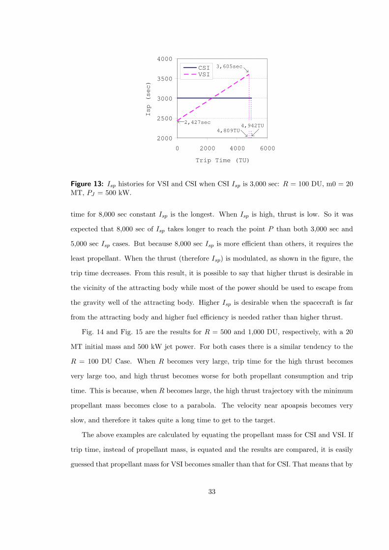
2000
2500
3000
3500
4000
0 2000 4000 6000
Trip Time (TU)
Isp (sec)
CSI VSI
2,427sec
3,605sec
4,942TU 4,809TU
Figure 13: Isp histories for VSI and CSI when CSI Isp is 3,000 sec: R = 100 DU, m0 = 20MT, PJ = 500 kW.
time for 8,000 sec constant Isp is the longest. When Isp is high, thrust is low. So it was
expected that 8,000 sec of Isp takes longer to reach the point P than both 3,000 sec and
5,000 sec Isp cases. But because 8,000 sec Isp is more efficient than others, it requires the
least propellant. When the thrust (therefore Isp) is modulated, as shown in the figure, the
trip time decreases. From this result, it is possible to say that higher thrust is desirable in
the vicinity of the attracting body while most of the power should be used to escape from
the gravity well of the attracting body. Higher Isp is desirable when the spacecraft is far
from the attracting body and higher fuel efficiency is needed rather than higher thrust.
Fig. 14 and Fig. 15 are the results for R = 500 and 1,000 DU, respectively, with a 20
MT initial mass and 500 kW jet power. For both cases there is a similar tendency to the
R = 100 DU Case. When R becomes very large, trip time for the high thrust becomes
very large too, and high thrust becomes worse for both propellant consumption and trip
time. This is because, when R becomes large, the high thrust trajectory with the minimum
propellant mass becomes close to a parabola. The velocity near apoapsis becomes very
slow, and therefore it takes quite a long time to get to the target.
The above examples are calculated by equating the propellant mass for CSI and VSI. If
trip time, instead of propellant mass, is equated and the results are compared, it is easily
guessed that propellant mass for VSI becomes smaller than that for CSI. That means that by
33
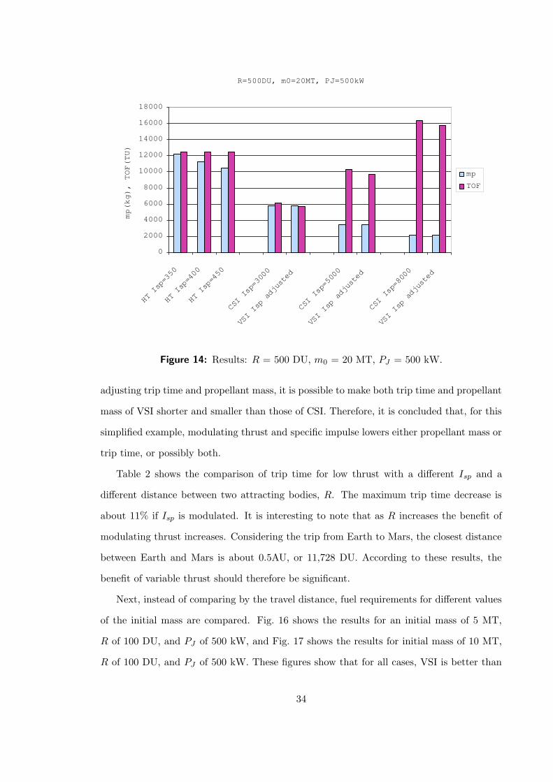
R=500DU, m0=20MT, PJ=500kW
0
2000
4000
6000
8000
10000
12000
14000
16000
18000
HT Isp=350
HT Isp=400
HT Isp=450
CSI Isp=3000
VSI Isp adjusted
CSI Isp=5000
VSI Isp adjusted
CSI Isp=8000
VSI Isp adjusted
mp(kg), TOF(TU)
mp
TOF
Figure 14: Results: R = 500 DU, m0 = 20 MT, PJ = 500 kW.
adjusting trip time and propellant mass, it is possible to make both trip time and propellant
mass of VSI shorter and smaller than those of CSI. Therefore, it is concluded that, for this
simplified example, modulating thrust and specific impulse lowers either propellant mass or
trip time, or possibly both.
Table 2 shows the comparison of trip time for low thrust with a different Isp and a
different distance between two attracting bodies, R. The maximum trip time decrease is
about 11% if Isp is modulated. It is interesting to note that as R increases the benefit of
modulating thrust increases. Considering the trip from Earth to Mars, the closest distance
between Earth and Mars is about 0.5AU, or 11,728 DU. According to these results, the
benefit of variable thrust should therefore be significant.
Next, instead of comparing by the travel distance, fuel requirements for different values
of the initial mass are compared. Fig. 16 shows the results for an initial mass of 5 MT,
R of 100 DU, and PJ of 500 kW, and Fig. 17 shows the results for initial mass of 10 MT,
R of 100 DU, and PJ of 500 kW. These figures show that for all cases, VSI is better than
34
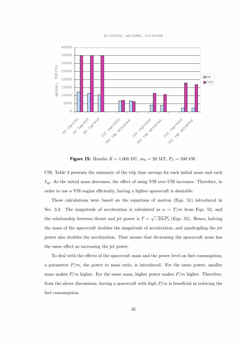
R=1000DU, m0=20MT, PJ=500kW
0
5000
10000
15000
20000
25000
30000
35000
40000
HT Isp=350
HT Isp=400
HT Isp=450
CSI Isp=3000
VSI Isp adjusted
CSI Isp=5000
VSI Isp adjusted
CSI Isp=8000
VSI Isp adjusted
mp(kg), TOF(TU)
mp
TOF
Figure 15: Results R = 1,000 DU, m0 = 20 MT, PJ = 500 kW.
CSI. Table 3 presents the summary of the trip time savings for each initial mass and each
Isp. As the initial mass decreases, the effect of using VSI over CSI increases. Therefore, in
order to use a VSI engine efficiently, having a lighter spacecraft is desirable.
These calculations were based on the equations of motion (Eqn. 51) introduced in
Sec. 3.3. The magnitude of acceleration is calculated as a = T/m from Eqn. 52, and
the relationship between thrust and jet power is T =√−2mPJ (Eqn. 55). Hence, halving
the mass of the spacecraft doubles the magnitude of acceleration, and quadrupling the jet
power also doubles the acceleration. That means that decreasing the spacecraft mass has
the same effect as increasing the jet power.
To deal with the effects of the spacecraft mass and the power level on fuel consumption,
a parameter P/m, the power to mass ratio, is introduced. For the same power, smaller
mass makes P/m higher. For the same mass, higher power makes P/m higher. Therefore,
from the above discussions, having a spacecraft with high P/m is beneficial in reducing the
fuel consumption.
35
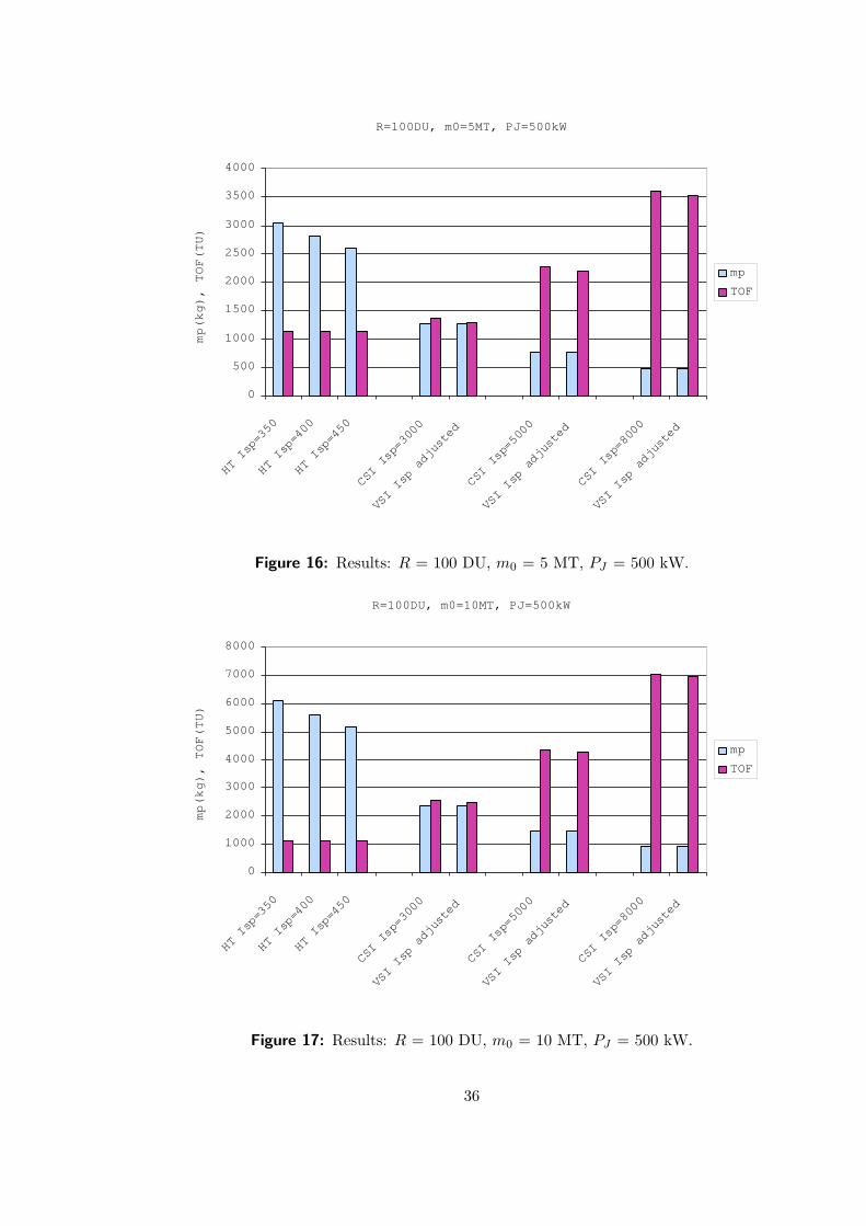
R=100DU, m0=5MT, PJ=500kW
0
500
1000
1500
2000
2500
3000
3500
4000
HT Isp=350
HT Isp=400
HT Isp=450
CSI Isp=3000
VSI Isp adjusted
CSI Isp=5000
VSI Isp adjusted
CSI Isp=8000
VSI Isp adjusted
mp(kg), TOF(TU)
mp
TOF
Figure 16: Results: R = 100 DU, m0 = 5 MT, PJ = 500 kW.
R=100DU, m0=10MT, PJ=500kW
0
1000
2000
3000
4000
5000
6000
7000
8000
HT Isp=350
HT Isp=400
HT Isp=450
CSI Isp=3000
VSI Isp adjusted
CSI Isp=5000
VSI Isp adjusted
CSI Isp=8000
VSI Isp adjusted
mp(kg), TOF(TU)
mp
TOF
Figure 17: Results: R = 100 DU, m0 = 10 MT, PJ = 500 kW.
36
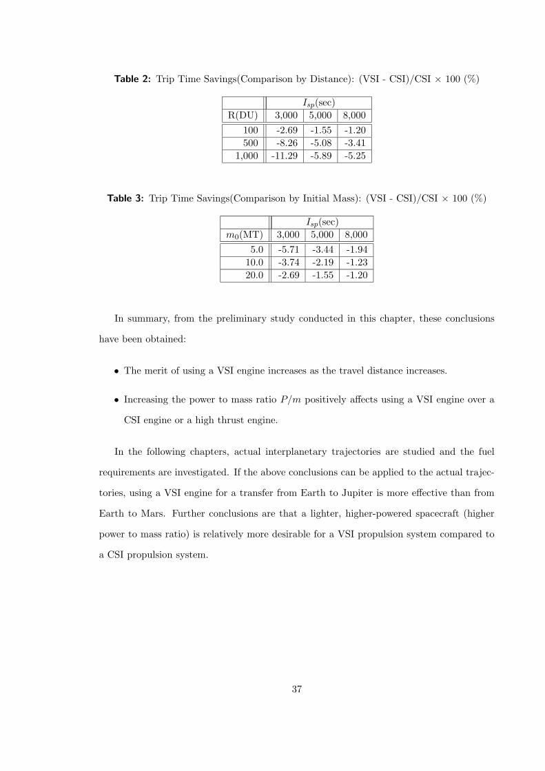
Table 2: Trip Time Savings(Comparison by Distance): (VSI - CSI)/CSI × 100 (%)
Isp(sec)
R(DU) 3,000 5,000 8,000
100 -2.69 -1.55 -1.20
500 -8.26 -5.08 -3.41
1,000 -11.29 -5.89 -5.25
Table 3: Trip Time Savings(Comparison by Initial Mass): (VSI - CSI)/CSI × 100 (%)
Isp(sec)
m0(MT) 3,000 5,000 8,000
5.0 -5.71 -3.44 -1.94
10.0 -3.74 -2.19 -1.23
20.0 -2.69 -1.55 -1.20
In summary, from the preliminary study conducted in this chapter, these conclusions
have been obtained:
• The merit of using a VSI engine increases as the travel distance increases.
• Increasing the power to mass ratio P/m positively affects using a VSI engine over a
CSI engine or a high thrust engine.
In the following chapters, actual interplanetary trajectories are studied and the fuel
requirements are investigated. If the above conclusions can be applied to the actual trajec-
tories, using a VSI engine for a transfer from Earth to Jupiter is more effective than from
Earth to Mars. Further conclusions are that a lighter, higher-powered spacecraft (higher
power to mass ratio) is relatively more desirable for a VSI propulsion system compared to
a CSI propulsion system.
37
CHAPTER V
INTERPLANETARY TRAJECTORY OPTIMIZATION
PROBLEMS
5.1 Assumptions
Consider a spacecraft travelling from one planet to another. The spacecraft, leaving from
the departure planet, must control its thrust direction to reach the target planet. In addition
to the thrust direction, a VSI engine should control its thrust magnitude, and a CSI engine
that is capable of turning the engine on/off should control the switching times.
Normally, a spacecraft launched from the ground with a launch vehicle takes either one
of the following steps.
• If the launch vehicle is not powerful enough or the spacecraft needs docking or other
on-orbit operations, the spacecraft is placed in Earth orbit at first, and then it boosts
to escape the Earth’s gravity well.
• If the launch vehicle has enough power to send the spacecraft out of the Earth’s gravity
well, the spacecraft flies directly to the target.
In either case, at first the spacecraft’s motion is affected by the Earth’s gravitational
force. Then as the spacecraft goes farther away from Earth, the gravitational force from
the Earth becomes smaller and the force from the Sun becomes dominant.
In actual missions, while the spacecraft is travelling from one planet to another, it
is subject to various forces including its own thrust, a gravitational force from the Sun,
and gravitational forces from all the planets and satellites, and other planetary bodies.
However, most of those forces are very small compared to the forces from the Sun or nearby
planets, and therefore most of the forces can be neglected. For example, a gravitational
force from Pluto affecting a spacecraft travelling from Earth to Mars is too small and it can
be neglected.
38
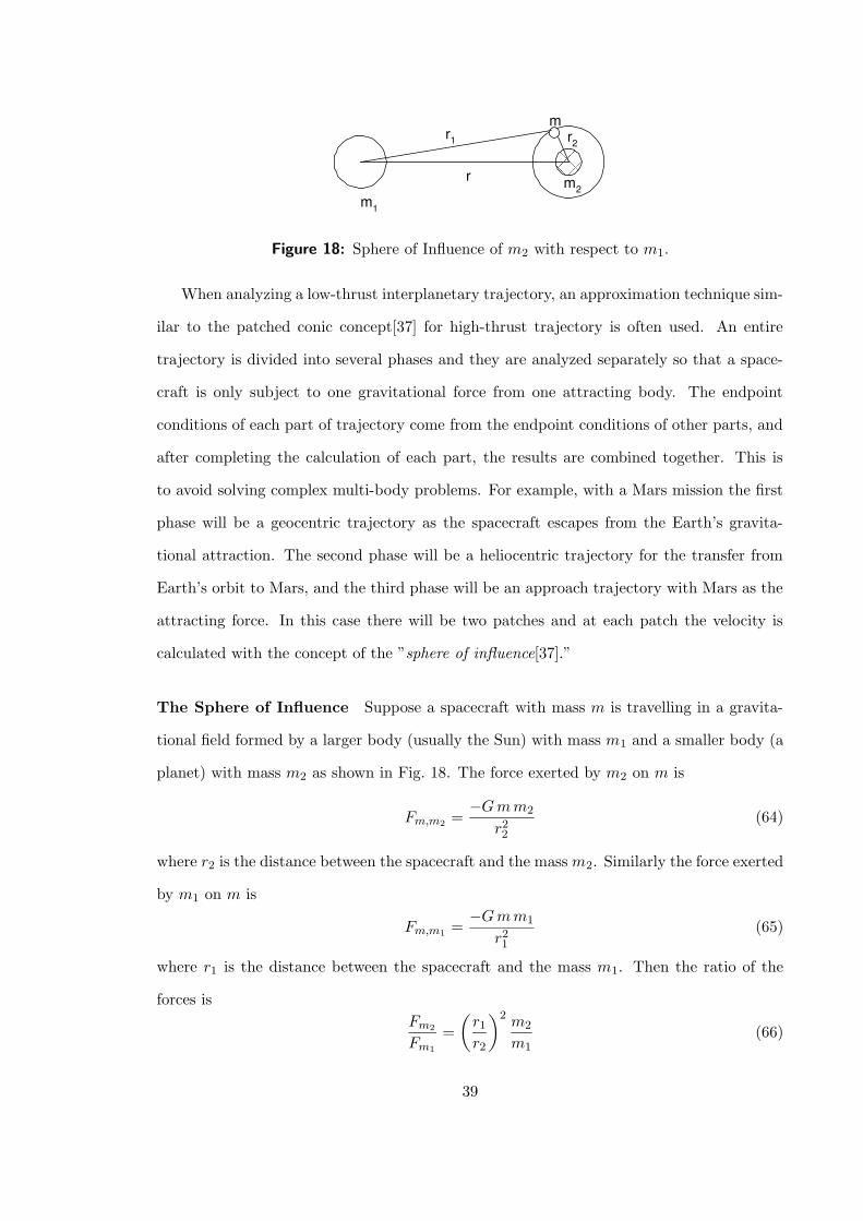
r 1 r 2
m 1
m 2 r
m
Figure 18: Sphere of Influence of m2 with respect to m1.
When analyzing a low-thrust interplanetary trajectory, an approximation technique sim-
ilar to the patched conic concept[37] for high-thrust trajectory is often used. An entire
trajectory is divided into several phases and they are analyzed separately so that a space-
craft is only subject to one gravitational force from one attracting body. The endpoint
conditions of each part of trajectory come from the endpoint conditions of other parts, and
after completing the calculation of each part, the results are combined together. This is
to avoid solving complex multi-body problems. For example, with a Mars mission the first
phase will be a geocentric trajectory as the spacecraft escapes from the Earth’s gravita-
tional attraction. The second phase will be a heliocentric trajectory for the transfer from
Earth’s orbit to Mars, and the third phase will be an approach trajectory with Mars as the
attracting force. In this case there will be two patches and at each patch the velocity is
calculated with the concept of the ”sphere of influence[37].”
The Sphere of Influence Suppose a spacecraft with mass m is travelling in a gravita-
tional field formed by a larger body (usually the Sun) with mass m1 and a smaller body (a
planet) with mass m2 as shown in Fig. 18. The force exerted by m2 on m is
Fm,m2=
−Gmm2
r22
(64)
where r2 is the distance between the spacecraft and the mass m2. Similarly the force exerted
by m1 on m is
Fm,m1=
−Gmm1
r21
(65)
where r1 is the distance between the spacecraft and the mass m1. Then the ratio of the
forces is
Fm2
Fm1
=
(
r1r2
)2 m2
m1
(66)
39
The sphere of influence (or SOI) is defined as the region in which the force exerted by the
smaller mass, m2, is much greater than that exerted on m by m1, we can think of the edge
of the SOI at r2 as being established when the ratio of the forces is approximately a tenth
(Fm1/Fm2
∼= 0.1). The approximate expression for the radius of the SOI is then
r2 ≈ r
(
10m2
m1
)0.5
(67)
where r is the distance between mass m1 and mass m2. Usually the radius of the SOI is
expressed in the following empirical manner:
rSOI = r
(
m2
m1
)0.4
(68)
For example, the radius of the SOI for the Earth with respect to the Sun can be calculated
as 0.00618 AU or 924,500 km using Eqn. 68.
Suppose that, a spacecraft is launched and when it reaches the edge of the SOI and it
has a velocity VEsc with respect to Earth, whose velocity is VSun
E with respect to the Sun.
Then the spacecraft’s velocity with respect to the Sun at this moment is
VSunsc = VSun
E +R[E → Sun]VEsc (69)
where R[E → Sun] is a transformation matrix from the Earth-centered coordinates to the
heliocentric coordinates. The spacecraft velocity with respect to Earth at the SOI, VEsc, is
often written as V∞.
In this research, instead of calculating V∞ by integrating the equations of motions inside
the sphere of influence, the planet’s gravity is ignored, and a parameter C3 is used. This is
the square of V∞ (√C3 = V∞) and expresses the twice of the kinetic energy of the spacecraft
per unit mass (km2/s2) at the edge of the SOI. This C3 value is often given as a launch
vehicle parameter, and with this value V∞ is calculated, and then the initial velocity of the
spacecraft with respect to the Sun is calculated with Eqn. 69. And even if the magnitude
of C3 is the same for two missions, the velocity of the spacecraft with respect to the Sun
may be different because the direction of the motion of the spacecraft at the edge of the
SOI may be different.
40
As for the position of the spacecraft with respect to the Sun when it is the edge of the
Earth’s SOI, another approximation is usually taken by assuming that the spacecraft is at
the center of the Earth. As shown above, the radius of the SOI for the Earth is 0.00618AU,
the error induced by this approximation is considered to be small enough to be neglected.
The same discussion is applied to the arrival planet. Final velocity at the arrival planet
is calculated by the predetermined C3 value. The final position is set to be the center of the
arrival planet at the moment. Of course in real life the spacecraft may circularize around
the planet and/or land on the ground after complicated operations, but these schemes are
not dealt with this research.
Therefore, in this research, the planetocentric phases are neglected and only interplan-
etary trajectories are considered. That means that the spacecraft is first placed in the
position where the Earth’s center exists, and its velocity is calculated by the C3 and the ve-
locity of the Earth. The spacecraft departs from the Earth’s position with Earth’s velocity
without gravitational pull from Earth as if there is no Earth.
We should be careful when neglecting planetocentric phases. When using low thrust
propulsion systems, it may take a long time and require some amount of fuel to escape from
the departure planet’s gravity well. Time and fuel may also be required for orbital insertion
at the arrival planet. The time of flight in this research does not include these times of
flight for spiral-in and spiral-out phases. The fuel requirements are also neglected for these
phases.
The spacecraft controls in-plane thrust angle and the out-of-plane thrust angle to reach
the target planet. For a VSI engine, thrust magnitude is also a control variable in addition
to thrust direction.
At the end of the mission, the target position is the center of the planet, and the final
velocity is calculated from C3 at the target planet and the velocity of the target planet with
respect to the Sun.
Another approximation used in this research is that the spacecraft is assumed to be a
point mass ejecting fuel from it to gain thrust. There is no attitude control problem, and
41
the thrust direction is assumed to be able to turn instantaneously.
With those approximations and assumptions stated above, for a given time of flight, the
fuel consumption is calculated for each type of engine and for each mission.
To express the state of the spacecraft, x, y, z components of position and velocity vectors
in the Cartesian coordinates are used.
x = u (70)
y = v (71)
z = w (72)
u = −µxr3
+Txm
(73)
v = −µyr3
+Tym
(74)
w = −µzr3
+Tzm
(75)
where µ is the gravitational constant, r = (x2+y2+z2)1/2; Tx, Ty, and Tz are the components
of the thrust; m is the mass of the spacecraft at the moment.
The merit of using this set of state variables are that these can be used for any type of
trajectory (elliptic, parabolic, or hyperbolic).
There are some other sets of variables that express the state of the spacecraft such as the
six classical orbital elements (the semi-major axis a, the eccentricity e, the inclination i, the
longitude of ascending node Ω, the argument of periapsis ω, and the mean anomaly M) or
equinoctial orbital elements (a = a, h = e sin(ω + Ω), k = e cos(ω + Ω), p = tan(i/2) sin Ω,
q = tan(i/2) cos Ω, and L = ν + ω + Ω)[13]. The equations of motion with the classical
orbital elements can not be used for a trajectory if the inclination is zero or 180 degrees.
The equations with the equinoctial orbital elements can be used only when the eccentricity
is less than one.
In this research, a trajectory with its inclination of zero or 180 degrees may be met with,
so the six classical orbital elements are not desirable. Also, because there is a possibility for
a trajectory to become hyperbolic, equinoctial orbital elements cannot be used. Therefore in
this research, position and velocity vectors in the Cartesian coordinates are used to express
the equations of motion of the spacecraft.
42
5.2 Equations of Motion for Low Thrust Trajectories
From rocket propulsion fundamentals and using Newton’s law for a variable mass body, the
equation of motion of a spacecraft is
m~r = m~c+m~g (76)
where ~r is the vehicle position vector, ~g is the acceleration of gravity, ~c is the exhaust
velocity, and m is mass flow rate.
This equation of motion is expressed by a set of differential equations for a position
vector ~r = [x y z]T and a velocity vector ~V = [u v w]T . The spacecraft’s mass is also
obtained by a differential equation for mass m.
f =
~r
~V
m
=
~V
−µ~r/r3 + ~T/m
−T 2/2PJ
(77)
In this research, the expression for the thrust vector ~T = [Tx Ty Tz]T differs depend-
ing on the problem so that each problem is solved most effectively.
5.2.1 VSI – No Constraints on Isp
For this problem, control variables are the same as the components of the thrust vector.
~u =
u0
u1
u2
=
Tx
Ty
Tz
(78)
Then the equations of motion are
f =
x
y
z
u
v
w
m
=
u
v
w
−µx/r3 + Tx/m
−µy/r3 + Ty/m
−µz/r3 + Tz/m
−(T 2x + T 2
y + T 2z )/2PJ
(79)
43
This type of problem can be solved with the method explained in 2.3.2.
5.2.2 VSI – Inequality Constraints on Isp
For this type of problem, we use the following control variables:
~u =
u0
u1
u2
u3
=
lx
ly
lz
T
(80)
where T is the magnitude of thrust, lx, ly, lz are the direction cosines of the direction of
thrust in the inertial frame, and are subject to l2x + l2y + l2z = 1. Then the equations of
motion are
f =
~r
~V
m
=
~V
−µ~r/r3 +~lT/m
−T 2/2PJ .
(81)
The Hamiltonian of this system is
H = ~λr · ~V − µ
r3~λV · ~r +~l · ~λV T/m− λmT
2/2PJ
= ~λr · ~V − µ
r3~λV · ~r − λm
2PJ
(
T −~l · ~λV PJmλm
)2
+(~l · ~λV )2PJ
2m2λm. (82)
According to the Pontryagin’s maximum principle, the thrust vector must be selected in
such a manner so as to maximize H at each instant of time. Therefore, we choose ~l parallel
to ~λV . Then ~l and T are expressed as
~l =
[
lx ly lz
]T
= ~λV /λV , ~λV =
[
λu λv λw
]T
(83)
T =PJλVmλm
(84)
The vector ~l is called the primer vector. The equations of motion and the control vector
44
are
f =
x
y
z
u
v
w
m
=
u
v
w
−µx/r3 + lxT/m
−µy/r3 + lyT/m
−µz/r3 + lzT/m
−T 2/2PJ
, ~u =
u0
u1
u2
u3
=
lx
ly
lz
T
. (85)
Therefore, solving this type of problem is the same as finding the Lagrange multipliers.
5.2.3 CSI – Continuous Thrust
For continuous thrust, the propellant mass is proportional to the time of flight. That
means that for a fixed time of flight the propellant mass does not change. The problems
dealt in this research are fixed time problems, so the propellant mass cannot be used as the
performance index. For this type of problem, the following performance index is used:
J = (u(tf ) − utarget)2 + (v(tf ) − vtarget)
2 + (w(tf ) − wtarget)2 (86)
and the terminal constraints are
ψ =
x(tf ) − xtarget
y(tf ) − ytarget
z(tf ) − ztarget
= 0. (87)
Because the thrust magnitude is fixed, there are two control variables.
~u =
u0
u1
=
θ
φ
(88)
where θ and φ are in-plane thrust angle and out-of-plane thrust angle in the inertial frame
as shown in
45
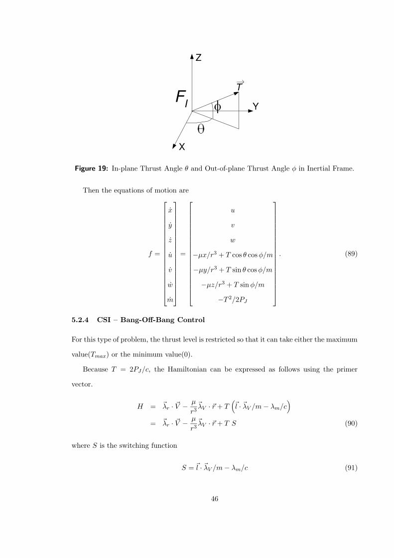
X
Y
Z
T F I
Figure 19: In-plane Thrust Angle θ and Out-of-plane Thrust Angle φ in Inertial Frame.
Then the equations of motion are
f =
x
y
z
u
v
w
m
=
u
v
w
−µx/r3 + T cos θ cosφ/m
−µy/r3 + T sin θ cosφ/m
−µz/r3 + T sinφ/m
−T 2/2PJ
. (89)
5.2.4 CSI – Bang-Off-Bang Control
For this type of problem, the thrust level is restricted so that it can take either the maximum
value(Tmax) or the minimum value(0).
Because T = 2PJ/c, the Hamiltonian can be expressed as follows using the primer
vector.
H = ~λr · ~V − µ
r3~λV · ~r + T
(
~l · ~λV /m− λm/c)
= ~λr · ~V − µ
r3~λV · ~r + T S (90)
where S is the switching function
S = ~l · ~λV /m− λm/c (91)
46
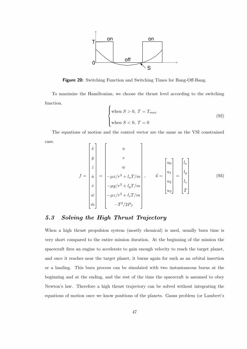
T
0
on
off
S
on
Figure 20: Switching Function and Switching Times for Bang-Off-Bang.
To maximize the Hamiltonian, we choose the thrust level according to the switching
function.
when S > 0, T = Tmax
when S < 0, T = 0
(92)
The equations of motion and the control vector are the same as the VSI constrained
case.
f =
x
y
z
u
v
w
m
=
u
v
w
−µx/r3 + lxT/m
−µy/r3 + lyT/m
−µz/r3 + lzT/m
−T 2/2PJ
, ~u =
u0
u1
u2
u3
=
lx
ly
lz
T
(93)
5.3 Solving the High Thrust Trajectory
When a high thrust propulsion system (mostly chemical) is used, usually burn time is
very short compared to the entire mission duration. At the beginning of the mission the
spacecraft fires an engine to accelerate to gain enough velocity to reach the target planet,
and once it reaches near the target planet, it burns again for such as an orbital insertion
or a landing. This burn process can be simulated with two instantaneous burns at the
beginning and at the ending, and the rest of the time the spacecraft is assumed to obey
Newton’s law. Therefore a high thrust trajectory can be solved without integrating the
equations of motion once we know positions of the planets. Gauss problem (or Lambert’s
47
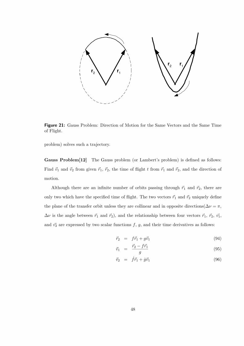
r 1 r 2
r 1 r 2
Figure 21: Gauss Problem: Direction of Motion for the Same Vectors and the Same Timeof Flight.
problem) solves such a trajectory.
Gauss Problem[12] The Gauss problem (or Lambert’s problem) is defined as follows:
Find ~v1 and ~v2 from given ~r1, ~r2, the time of flight t from ~r1 and ~r2, and the direction of
motion.
Although there are an infinite number of orbits passing through ~r1 and ~r2, there are
only two which have the specified time of flight. The two vectors ~r1 and ~r2 uniquely define
the plane of the transfer orbit unless they are collinear and in opposite directions(∆ν = π,
∆ν is the angle between ~r1 and ~r2), and the relationship between four vectors ~r1, ~r2, ~v1,
and ~v2 are expressed by two scalar functions f , g, and their time derivatives as follows:
~r2 = f~r1 + g~v1 (94)
~v1 =~r2 − f~r1
g(95)
~v2 = f~r1 + g~v1 (96)
48
where
f = 1 − r2p
(1 − cos ∆ν) = 1 − a
r1(1 − cos ∆E) (97)
g =r1r2 sin ∆ν√
µp= t−
√
a3
µ(∆E − sin ∆E) (98)
f =
√
µ
ptan
∆ν
2
(
1 − cos ∆ν
p− 1
r1− 1
r2
)
=−√
µa
r1r2sin ∆E (99)
g = 1 − r1p
(1 − cos ∆ν) = 1 − a
r2(1 − cos ∆E). (100)
Here a is semi-major axis, p is semi-latus rectum, and ∆E is difference of the eccentric
anomaly that corresponds to ∆ν.
The above expression is not for any conic section but only for ellipse because the eccentric
anomaly E is defined only when the eccentricity is less than one.
To solve trajectories with any eccentricity, another expression is required. For this
research “Solution via universal variables” is used.
Solution via Universal Variables[12] Using universal variables x and z, Eqn. 97 to
100 are expressed as follows:
f = 1 − r2p
(1 − cos ∆ν) = 1 − x2
r1C (101)
g =r1r2 sin ∆ν√
µp= t− x3
õS (102)
f =
√
µ
p
(1 − cos ∆ν)
sin ∆ν
(
1 − cos ∆ν
p− 1
r1− 1
r2
)
= −√µ
r1r2x(1 − zS) (103)
g = 1 − r1p
(1 − cos ∆ν) = 1 − x2
r2C. (104)
Solving for x from Eqn. 101, we get
x =
√
r1r2(1 − cos ∆ν)
p C. (105)
Substituting for x in Eqn. 103 and cancelling√
µ/p from both sides, yields,
1 − cos ∆ν
sin ∆ν
(
1 − cos∆ν
p− 1
r1− 1
r2
)
= −√
1 − cos ∆ν
r1r2
(1 − zS)√C
. (106)
If we multiply both sides by r1r2 and rearrange, the following expression is obtained:
r1r2(1 − cos ∆ν)
p= r1 + r2 −
√r1r2 sin ∆ν√1 − cos ∆ν
(1 − zS)√C
. (107)
49
If we define parameters A and y as
A =
√r1r2 sin ∆ν√1 − cos ∆ν
(108)
y =r1r2(1 − cos ∆ν)
p= r1 + r2 −A
(1 − zS)√C
, (109)
x is expressed as
x =
√
y
C(110)
and Eqn. 102 becomes
õ t = x3S +
r1r2 sin ∆ν√p
= x3S +A√y. (111)
Then equations 101, 102, and 104 become
f = 1 − y
r1(112)
g = A
√
y
µ(113)
g = 1 − y
r2(114)
Since ~r2 = f~r1 + g~v1, ~v1 and ~v2 can be computed as
~v1 =~r2 − f~r1
g(115)
~v2 = f~r1 + g~v1 =g~r2 − ~r1
g. (116)
The numerical method of computing the Gauss problem is explained in the next chapter.
5.4 Problems with Swing-by
5.4.1 Mechanism
The use of swing-by is a technique that is referred to as “gravity assist”[37]. Studies of
interplanetary flight with gravity assist maneuvers are known to deal with cases where the
spacecraft on its way from one celestial body to another approaches a third attracting body,
which brings about a significant change in the spacecraft trajectory[53]. The use of swing-by
may reduce the propulsive velocity budget, and the mechanism is explained in the following
manner.
50
Assume a spacecraft entering an SOI of a planet with incoming velocity V∞i, a velocity
vector with respect to the planet. V∞ican be expressed as V∞i
= VHi −VH
pl , where VHi is
the heliocentric velocity of the spacecraft and VHpl is the heliocentric velocity of the planet.
If no propulsive force is added, the energy of the swing-by trajectory with respect to the
swing-by planet remains constant, so the magnitude of the outgoing velocity magnitude
V∞o is equal to the incoming velocity magnitude V∞i(= |V∞i
|) but the direction has been
changed. Therefore, the outgoing “heliocentric” velocity VHo (= V∞o + VH
pl ) is not equal
to VHi , in both magnitude and direction. That means the spacecraft either increases or
decreases its energy with a planetary swing-by. Using the equation of the conservation of
the energy:
msc∆Esc +mpl∆Epl = 0 (117)
where msc and mpl are the mass of spacecraft and planet, and ∆Epl and ∆Esc are the
energy change due to the swing-by for spacecraft and planet, respectively, then the energy
the spacecraft gained is
∆Esc = −mpl
msc∆Epl. (118)
A Mercury swing-by produces the largest energy change because of its highest heliocen-
tric velocity among all planets, and a Jupiter swing-by gives the largest trajectory deflection
for a given V∞ because of its largest mass.
Next, general expressions for the planetary swing-by are developed.
5.4.2 Equations of Motion
Suppose that the position and velocity of the spacecraft in the heliocentric coordinate system
(~r hsc1 and ~V hsc1) are known at the moment (time t1). It enters the sphere of influence of a
swing-by body whose position in the heliocentric coordinates is ~r hpl1 = ~rpl(t1) and velocity
is ~V hpl1 = ~Vpl(t1)(see Fig. 22)[53].
The coordinates are transferred from heliocentric coordinates to planetocentric coordi-
nates and the position and velocity vector of the spacecraft with respect to the swing-by
51
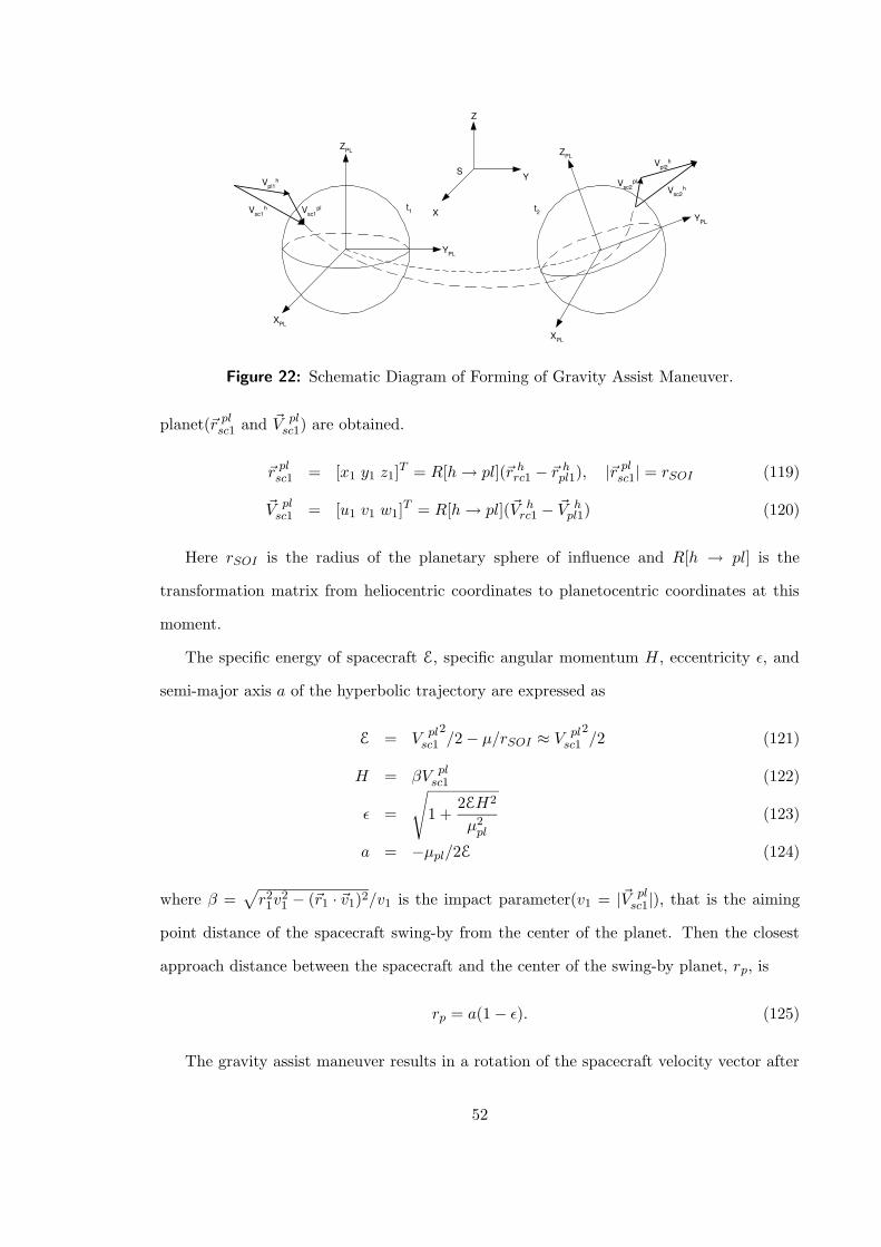
Z
Y S
X
Z PL
X PL
Y PL
Z PL
Y PL
X PL
t 1 t 2
V pl1 h
V sc1 h V sc1
pl
V pl2 h
V sc2 h
V sc2 pl
Figure 22: Schematic Diagram of Forming of Gravity Assist Maneuver.
planet(~r plsc1 and ~V plsc1) are obtained.
~r plsc1 = [x1 y1 z1]T = R[h→ pl](~r hrc1 − ~r hpl1), |~r plsc1| = rSOI (119)
~V plsc1 = [u1 v1 w1]
T = R[h→ pl](~V hrc1 − ~V h
pl1) (120)
Here rSOI is the radius of the planetary sphere of influence and R[h → pl] is the
transformation matrix from heliocentric coordinates to planetocentric coordinates at this
moment.
The specific energy of spacecraft E, specific angular momentum H, eccentricity ε, and
semi-major axis a of the hyperbolic trajectory are expressed as
E = V plsc1
2/2 − µ/rSOI ≈ V pl
sc1
2/2 (121)
H = βV plsc1 (122)
ε =
√
1 +2EH2
µ2pl
(123)
a = −µpl/2E (124)
where β =√
r21v21− (~r1 · ~v1)2/v1 is the impact parameter(v1 = |~V pl
sc1|), that is the aiming
point distance of the spacecraft swing-by from the center of the planet. Then the closest
approach distance between the spacecraft and the center of the swing-by planet, rp, is
rp = a(1 − ε). (125)
The gravity assist maneuver results in a rotation of the spacecraft velocity vector after
52
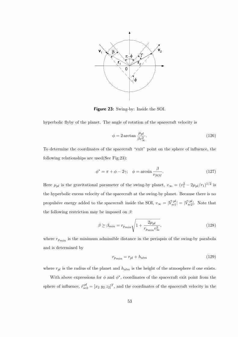
r 1 r 2
v 1 v 2
0
-
Figure 23: Swing-by: Inside the SOI.
hyperbolic flyby of the planet. The angle of rotation of the spacecraft velocity is
φ = 2 arctanµplβv2
∞
. (126)
To determine the coordinates of the spacecraft “exit” point on the sphere of influence, the
following relationships are used(See Fig.23):
φ∗ = π + φ− 2γ; φ = arcsinβ
rSOI. (127)
Here µpl is the gravitational parameter of the swing-by planet, v∞ = (v21 − 2µpl/r1)
1/2 is
the hyperbolic excess velocity of the spacecraft at the swing-by planet. Because there is no
propulsive energy added to the spacecraft inside the SOI, v∞ = |~V plsc1| = |~V pl
sc2|. Note that
the following restriction may be imposed on β:
β ≥ βmin = rpmin
√
1 +2µpl
rpminv2∞
, (128)
where rpmin is the minimum admissible distance in the periapsis of the swing-by parabola
and is determined by
rpmin = rpl + hatm (129)
where rpl is the radius of the planet and hatm is the height of the atmosphere if one exists.
With above expressions for φ and φ∗, coordinates of the spacecraft exit point from the
sphere of influence, ~r plsc2 = [x2 y2 z2]T , and the coordinates of the spacecraft velocity in the
53
planetocentric coordinate system, ~V plsc2 = [u2 v2 w2]
T , can be written as:
~r plsc2 =
x2
y2
z2
= Ω(φ∗)~r plsc1 = Ω(φ∗)
x1
y1
z1
(130)
~V plsc2 =
u2
v2
w2
= Ω(φ)~V plsc1 = Ω(φ)
u1
v1
w1
(131)
The transformation matrix Ω is written as
Ω =
hxhx(1 − cosφ) + cosφ hxhy(1 − cosφ) − hz sinφ hzhx(1 − cosφ) + hy sinφ
hxhy(1 − cosφ) + hz sinφ hyhy(1 − cosφ) + cosφ hyhz(1 − cosφ) − hx sinφ
hzhx(1 − cosφ) − hy sinφ hyhz(1 − cosφ) + hx sinφ hzhz(1 − cosφ) + cosφ
(132)
where [hx, hy, hz] are the unit vector of angular momentum, ~r plsc1 × ~V plsc1/|~r
plsc1 × ~V pl
sc1|.
The duration of the spacecraft motion in the swing-by planet’s sphere of influence can
be derived from
∆t = 2
√
a3
µpl
(
cscφ
2sinhH −H
)
(133)
coshH =(
1 +rSOIa
)
sinφ
2(134)
a =
(
v21
µpl− 2
rSOI
)−1
(135)
Therefore, the spacecraft, entering the sphere of influence at time t1 with position r hsc1
and velocity V hsc1 in the heliocentric coordinates, leaves the sphere of influence of the swing-
by planet at time t2 = t1 + ∆t whose position is ~r hpl2 = ~rpl(t2) and velocity is ~V hpl2 = ~Vpl(t2).
The spacecraft position r hsc2 and velocity V hsc2 at this moment (time t1) is expressed as
r hsc2 = ~r hpl2 +R[pl → h]~r plsc2 (136)
V hsc2 = ~V h
pl2 +R[pl → h] ~V plsc2 (137)
whereR[pl → h] is the transformation matrix from planetocentric coordinates to heliocentric
coordinates at this moment.
54
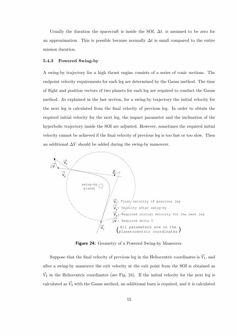
Usually the duration the spacecraft is inside the SOI, ∆t, is assumed to be zero for
an approximation. This is possible because normally ∆t is small compared to the entire
mission duration.
5.4.3 Powered Swing-by
A swing-by trajectory for a high thrust engine consists of a series of conic sections. The
endpoint velocity requirements for each leg are determined by the Gauss method. The time
of flight and position vectors of two planets for each leg are required to conduct the Gauss
method. As explained in the last section, for a swing-by trajectory the initial velocity for
the next leg is calculated from the final velocity of previous leg. In order to obtain the
required initial velocity for the next leg, the impact parameter and the inclination of the
hyperbolic trajectory inside the SOI are adjusted. However, sometimes the required initial
velocity cannot be achieved if the final velocity of previous leg is too fast or too slow. Then
an additional ∆V should be added during the swing-by maneuver.
V 1
V 2
V 3
V
: Final velocity of previous leg
: Velocity after swing-by
: Required initial velocity for the next leg
: Required delta V
V 1
V 3
V 2
V
swing-by planet
All parameters are in the planetocentric coordinates ( )
Figure 24: Geometry of a Powered Swing-by Maneuver.
Suppose that the final velocity of previous leg in the Heliocentric coordinates is ~V1, and
after a swing-by maneuver the exit velocity at the exit point from the SOI is obtained as
~V2 in the Heliocentric coordinates (see Fig. 24). If the initial velocity for the next leg is
calculated as ~V3 with the Gauss method, an additional burn is required, and it is calculated
55
as ∆~V = ~V3 − ~V2.
The only way to adjust ∆V is to adjust the entry point at the SOI because the final
velocity of previous leg cannot be adjusted. Therefore, finding the minimum ∆V for a high
thrust swing-by trajectory is equivalent to finding the proper entry point at the SOI.
56
CHAPTER VI
DEVELOPMENT OF THE APPLICATION “SAMURAI”
Using all of the techniques introduced through the last chapter and in the Appendix C, a
numerical analysis software application “SAMURAI” – Simulation and Animation Model
Used for Rockets with Adjustable Isp – has been developed in C++. SAMURAI simulates
interplanetary trajectories with different types of propulsion systems. In this chapter, ca-
pabilities of SAMURAI, classes implemented in SAMURAI, and the flow of calculation are
introduced. A full description of input data is in Appendix D.
6.1 Overview
6.1.1 Capabilities
SAMURAI is an interplanetary trajectory optimization application that calculates the
thrust history (thrust magnitude and direction) for a prescribed condition (initial posi-
tion and velocity, target position and velocity, and time of flight). Several types of engines
can be analyzed. SAMURAI utilizes a calculus of variations algorithm to evaluate the con-
trol history that minimizes the fuel consumption for a transfer trajectory from one planet
to another. A trajectory with a planetary swing-by can also be calculated.
SAMURAI directly integrates the equations of motion for a spacecraft to determine the
spacecraft’s path. Normally, low thrust applications employ perturbation techniques that
require the thrust level to be very small. Because SAMURAI does not use any perturbation
techniques, it can calculate trajectories with any thrust level.
The engine types SAMURAI can deal with are the following:
• VSI engine type I (variable thrust and variable Isp, no limit for Isp)
• VSI engine type II (variable thrust and variable Isp, with an upper limit for Isp)
• CSI engine type I (constant thrust and constant Isp, continuous burn)
57
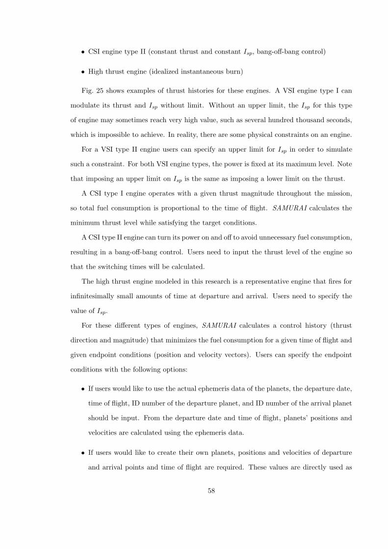
• CSI engine type II (constant thrust and constant Isp, bang-off-bang control)
• High thrust engine (idealized instantaneous burn)
Fig. 25 shows examples of thrust histories for these engines. A VSI engine type I can
modulate its thrust and Isp without limit. Without an upper limit, the Isp for this type
of engine may sometimes reach very high value, such as several hundred thousand seconds,
which is impossible to achieve. In reality, there are some physical constraints on an engine.
For a VSI type II engine users can specify an upper limit for Isp in order to simulate
such a constraint. For both VSI engine types, the power is fixed at its maximum level. Note
that imposing an upper limit on Isp is the same as imposing a lower limit on the thrust.
A CSI type I engine operates with a given thrust magnitude throughout the mission,
so total fuel consumption is proportional to the time of flight. SAMURAI calculates the
minimum thrust level while satisfying the target conditions.
A CSI type II engine can turn its power on and off to avoid unnecessary fuel consumption,
resulting in a bang-off-bang control. Users need to input the thrust level of the engine so
that the switching times will be calculated.
The high thrust engine modeled in this research is a representative engine that fires for
infinitesimally small amounts of time at departure and arrival. Users need to specify the
value of Isp.
For these different types of engines, SAMURAI calculates a control history (thrust
direction and magnitude) that minimizes the fuel consumption for a given time of flight and
given endpoint conditions (position and velocity vectors). Users can specify the endpoint
conditions with the following options:
• If users would like to use the actual ephemeris data of the planets, the departure date,
time of flight, ID number of the departure planet, and ID number of the arrival planet
should be input. From the departure date and time of flight, planets’ positions and
velocities are calculated using the ephemeris data.
• If users would like to create their own planets, positions and velocities of departure
and arrival points and time of flight are required. These values are directly used as
58
0 0.2 0.4 0.6 0.8 10
100
200
300
400
time (scaled)
thru
st (N
)
VSI unlimited Isp
0 0.2 0.4 0.6 0.8 10
100
200
300
400
time (scaled)
thru
st (N
)
VSI bounded Isp
0 0.2 0.4 0.6 0.8 10
100
200
300
400
time (scaled)
thru
st (N
)
CSI continuous
0 0.2 0.4 0.6 0.8 10
100
200
300
400
time (scaled)
thru
st (N
)
CSI bang−off−bang
0 0.2 0.4 0.6 0.8 10
1000
2000
3000
4000
time (scaled)
thru
st (N
)
High Thrust
Figure 25: Examples of Thrust Histories.
59
the endpoint conditions.
In addition to calculating the trajectory for one value of the departure date and time
of flight, SAMURAI has the capability to conduct a grid search with these two parameters
by specifying the range of each parameter. Then SAMURAI finds the best launch date and
time of flight for the given initial and final conditions.
Other input data required are jet power (W), initial mass (kg), and C3 values at depar-
ture and arrival which are introduced in Sec. 5.1. Optional data may be input such as the
maximum number of iterations or the tolerance for the convergence criteria to avoid a long
computation time and suboptimal results.
6.1.2 Performance Index for Each Engine
Since the target for VSI engines is to minimize fuel consumption, we would like to maximize
the mass at tf . Therefore, the performance index is expressed as the negative value of the
mass of spacecraft:
J = −m(tf ) (φ = −m(tf ) and L = 0), (138)
subject to the endpoint constraints:
x(ti)
y(ti)
z(ti)
u(ti)
v(ti)
w(ti)
are given, ψ = X(tf ) −Xtarget =
x(tf ) − xtarget
y(tf ) − ytarget
z(tf ) − ztarget
u(tf ) − utarget
v(tf ) − vtarget
w(tf ) − wtarget
= 0 (139)
x(ti), y(ti), and z(ti) are position components of the departure planet, and xtarget,
ytarget, and ztarget are position components of the arrival planet. If both C3’s at departure
and arrival are zero, Xtarget is the position and velocity of the arrival planet. If either one of
C3’s or both C3’s are nonzero, then the best thrust direction at the endpoints is calculated
so that it minimizes the fuel consumption. In such a case, u(ti), v(ti), w(ti), and utarget,
60
vtarget, wtarget are not the velocity components of the planets, but the sum of the planet’s
velocity and the velocity of the spacecraft with respect to the planet (V∞).
For CSI cases, because the fuel consumption is proportional to the flight time (tf − ti),
the spacecraft mass cannot be used as the performance index. Instead, the performance
index and constraints are defined as follows:
Minimize J =1
2
[
(u(tf ) − utarget)2 + (v(tf ) − vtarget)
2 + (w(tf ) − wtarget)2]
(140)
subject to
ψ =
x(tf ) − xtarget
y(tf ) − ytarget
z(tf ) − ztarget
= 0. (141)
Because the thrust magnitude is fixed for CSI, the control variables are just the components
of the thrust direction.
For CSI type I, the minimum thrust level is obtained through an iterative process. If the
target conditions are not satisfied with a trial thrust level, a new optimization is performed
with a new, slightly bigger thrust level. If the constraints are satisfied, then a calculation
with a lower thrust level is performed. This process is iterated until the minimum thrust
level that satisfies the constraints is found.
For CSI type II, a bang-off-bang thrust profile is created with the switching function
introduced in Sec. 5.2. Switching times (on → off and off → on) that satisfy Eqns. 138 and
139 are calculated.
For high thrust, the Gauss problem is solved to obtain the endpoint velocities for the
input time of flight. No optimization process is required unless the two endpoint vectors
are collinear. When the two endpoint vectors are collinear or almost collinear, endpoint
velocity vectors are computed using Powell’s moethod so that total ∆V is minimized.
6.2 C++ Classes
SAMURAI contains 20 classes. The important classes are introduced here.
• Appli class controls all of the classes. This class creates all the classes, initializes them,
61
and then starts calculation. After the minimum-fuel trajectory is obtained, Vrml class
is called and a VRML file is created.
• Inp class reads input data. All of the input parameters are checked and if an inap-
propriate parameter is found, it ends the program. In this class, all the input data is
converted into canonical units: km → DU, day or second → TU, kg → non-dimensional
etc.
• Calc class controls the grid search procedure and calculates the overall minimum-fuel
trajectory for an input range of departure date and time of flight. Departure date
and time of flight are set in this class, and they are sent to Mission class in which the
optimal trajectory for a given departure date and time of flight is calculated.
• Mission class controls the calculation of the minimum-fuel trajectory for the time
interval that is sent from Calc class. At first the planets’ positions and velocities are
calculated with Planet class. Then the spacecraft velocity at the initial point and final
point are calculated. These endpoint conditions are used as the initial condition and
the target condition of the optimization problem. An iterative procedure is required
until the minimum-fuel trajectory for the time interval is found.
• Phase class calculates the minimum-fuel trajectory for a given initial condition, final
condition, and time of flight sent from Mission class. This class is implemented for each
phase(trajectory from one planet to another). Therefore, for a swing-by trajectory
calculation, this class is called twice from Mission class.
• Powell class conducts Powell’s method. This class is used for several optimization
schemes as explained in Chap. C.
• Line class conducts a line search, using three-point quadratic approximations.
• Opt class handles optimal control processes with the first-order gradient algorithm.
From initial state variables and an initial guess of the control history, an optimal
control history that minimizes the cost function is calculated.
62
• Ode class solves ordinary differential equations with the Runge-Kutta method. With
state variables at initial time and histories of the control variables throughout the
propagation period, a history of state variables are calculated by integrating the dif-
ferential equations.
• Func class contains required functions. Differential equations for spacecraft’s equa-
tions of motion, the derivatives of these equations with respect to the state variables
and control variables, and other equations to conduct the optimization process are
stored in this class.
• HighThrust class calculates a high thrust trajectory using the Gauss method. From
two position vectors of planets and time of flight, velocity vectors at the initial and
final points are calculated. If the two position vectors are collinear, Powell’s method
is used to minimize the fuel requirement as explained in Chap. C.
• Planet class calculates a planet’s position and velocity. With the input Julian date,
the position and velocity at that instant are calculated using the functions stored in
this class.
• Swingby class controls the swing-by process. With the incoming velocity vector ob-
tained from phase 1 and a guessed value of the impact parameter, the outgoing velocity
vector is calculated. This velocity is used as the initial velocity of the transfer orbit
for phase 2. Powell’s method is used to find a set of the best incoming velocity vec-
tors and the entry point at the sphere of influence that minimizes the overall fuel
consumption.
• Vrml class creates a VRML file that draws an animation of the resulting optimal
trajectory on the web browser. This class converts the state variables and control
variables to the VRML format, and prints them out to a file.
63
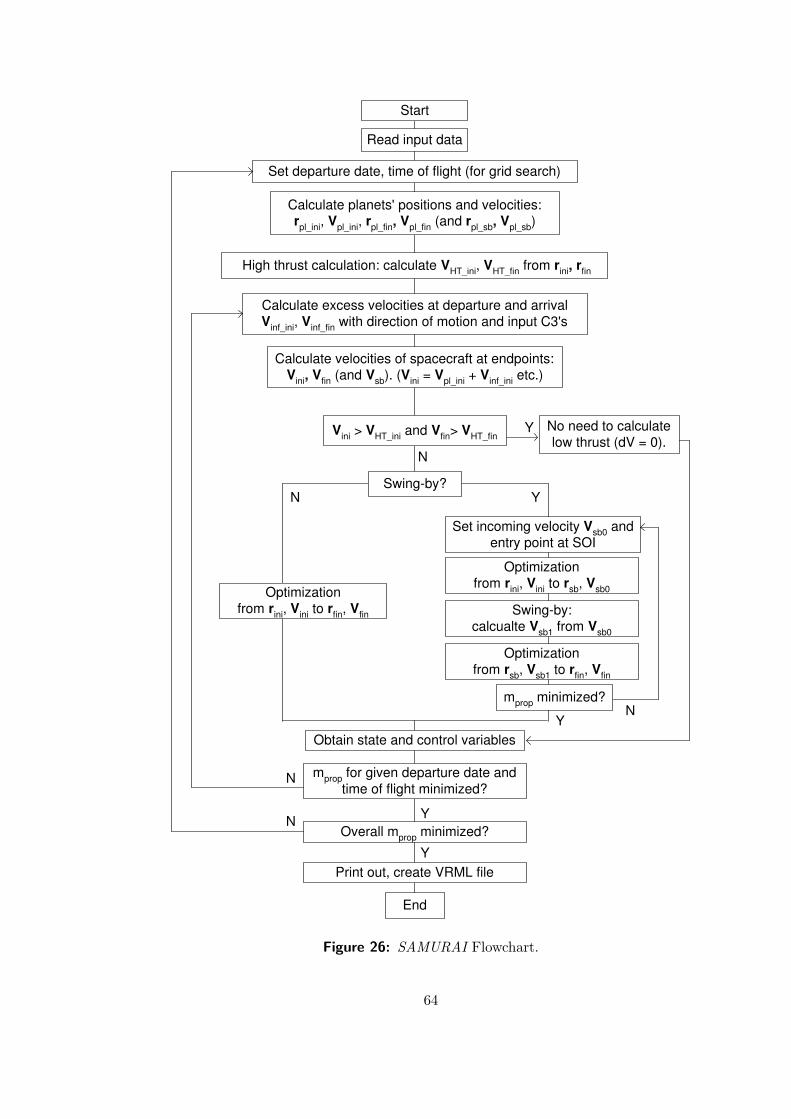
Start
Read input data
Set departure date, time of flight (for grid search)
Calculate planets' positions and velocities: r pl_ini , V pl_ini , r pl_fin , V pl_fin (and r pl_sb , V pl_sb )
Calculate velocities of spacecraft at endpoints: V ini , V fin (and V sb ). ( V ini = V pl_ini + V inf_ini etc.)
Calculate excess velocities at departure and arrival V inf_ini , V inf_fin with direction of motion and input C3's
High thrust calculation: calculate V HT_ini , V HT_fin from r ini , r fin
No need to calculate low thrust (dV = 0).
Swing-by?
Optimization from r ini , V ini to r fin , V fin
Optimization from r ini , V ini to r sb , V sb0
Optimization from r sb , V sb1 to r fin , V fin
Swing-by: calcualte V sb1 from V sb0
m prop minimized?
Set incoming velocity V sb0 and entry point at SOI
Obtain state and control variables
m prop for given departure date and time of flight minimized?
Overall m prop minimized?
Print out, create VRML file
End
N
Y
N Y
N
N Y
Y
Y N
V ini > V HT_ini and V fin > V HT_fin
Figure 26: SAMURAI Flowchart.
64
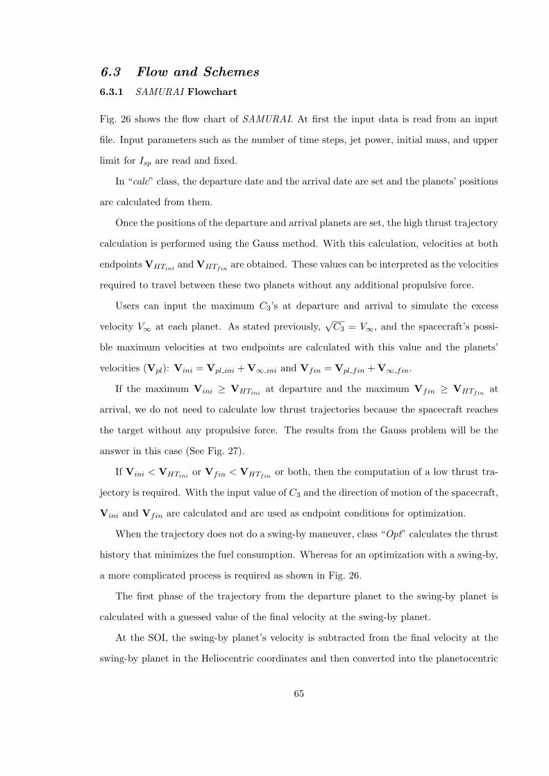
6.3 Flow and Schemes
6.3.1 SAMURAI Flowchart
Fig. 26 shows the flow chart of SAMURAI. At first the input data is read from an input
file. Input parameters such as the number of time steps, jet power, initial mass, and upper
limit for Isp are read and fixed.
In “calc” class, the departure date and the arrival date are set and the planets’ positions
are calculated from them.
Once the positions of the departure and arrival planets are set, the high thrust trajectory
calculation is performed using the Gauss method. With this calculation, velocities at both
endpoints VHTiniand VHTfin
are obtained. These values can be interpreted as the velocities
required to travel between these two planets without any additional propulsive force.
Users can input the maximum C3’s at departure and arrival to simulate the excess
velocity V∞ at each planet. As stated previously,√C3 = V∞, and the spacecraft’s possi-
ble maximum velocities at two endpoints are calculated with this value and the planets’
velocities (Vpl): Vini = Vpl ini + V∞ ini and Vfin = Vpl fin + V∞ fin.
If the maximum Vini ≥ VHTiniat departure and the maximum Vfin ≥ VHTfin
at
arrival, we do not need to calculate low thrust trajectories because the spacecraft reaches
the target without any propulsive force. The results from the Gauss problem will be the
answer in this case (See Fig. 27).
If Vini < VHTinior Vfin < VHTfin
or both, then the computation of a low thrust tra-
jectory is required. With the input value of C3 and the direction of motion of the spacecraft,
Vini and Vfin are calculated and are used as endpoint conditions for optimization.
When the trajectory does not do a swing-by maneuver, class “Opt” calculates the thrust
history that minimizes the fuel consumption. Whereas for an optimization with a swing-by,
a more complicated process is required as shown in Fig. 26.
The first phase of the trajectory from the departure planet to the swing-by planet is
calculated with a guessed value of the final velocity at the swing-by planet.
At the SOI, the swing-by planet’s velocity is subtracted from the final velocity at the
swing-by planet in the Heliocentric coordinates and then converted into the planetocentric
65
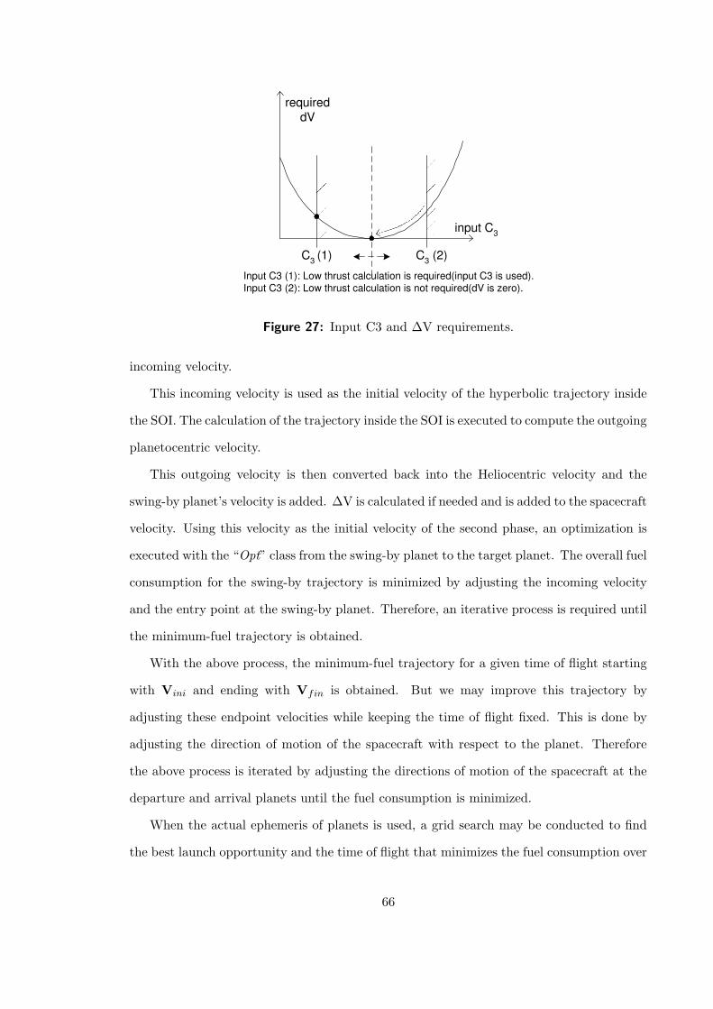
required dV
input C 3
C 3 (1) C 3 (2)
Input C3 (1): Low thrust calculation is required(input C3 is used). Input C3 (2): Low thrust calculation is not required(dV is zero).
Figure 27: Input C3 and ∆V requirements.
incoming velocity.
This incoming velocity is used as the initial velocity of the hyperbolic trajectory inside
the SOI. The calculation of the trajectory inside the SOI is executed to compute the outgoing
planetocentric velocity.
This outgoing velocity is then converted back into the Heliocentric velocity and the
swing-by planet’s velocity is added. ∆V is calculated if needed and is added to the spacecraft
velocity. Using this velocity as the initial velocity of the second phase, an optimization is
executed with the “Opt” class from the swing-by planet to the target planet. The overall fuel
consumption for the swing-by trajectory is minimized by adjusting the incoming velocity
and the entry point at the swing-by planet. Therefore, an iterative process is required until
the minimum-fuel trajectory is obtained.
With the above process, the minimum-fuel trajectory for a given time of flight starting
with Vini and ending with Vfin is obtained. But we may improve this trajectory by
adjusting these endpoint velocities while keeping the time of flight fixed. This is done by
adjusting the direction of motion of the spacecraft with respect to the planet. Therefore
the above process is iterated by adjusting the directions of motion of the spacecraft at the
departure and arrival planets until the fuel consumption is minimized.
When the actual ephemeris of planets is used, a grid search may be conducted to find
the best launch opportunity and the time of flight that minimizes the fuel consumption over
66
a range of departure dates and times of flight.
After all of the above process are finished, a VRML file that draws a 3D animation is
created.
6.3.2 VSI Constrained Isp
Finding an optimal solution for a VSI unconstrained Isp problem is relatively simple. The
1st-order gradient algorithm introduced in the previous chapter is suitable for this kind of
problem.
However, constrained cases are complicated and require more calculations than uncon-
strained cases. To solve VSI type II problems, the initial guess for the Lagrange multiplier
λ(ti) is required in order to estimate the control vector at initial time.
For VSI type II calculations, the results from VSI type I are used. This is because
the thrust histories are similar to each other for unconstrained arcs, and the Lagrange
multipliers obtained in VSI type I calculations should be used as an initial guess for VSI
type II calculation.
The following steps are taken to obtain the results for VSI type II.
1. Calculate a trajectory for VSI type I.
2. Obtain the Lagrange multipliers ~λ at initial time ti from the previous step.
3. From ~x and ~λ, calculate the control variables:
~l = [lx ly lz]T = ~λv/λv, T =
PJλVmλm
. (142)
4. Integrate x and λ forward from ti to final time tf with the control variables obtained
in the step 3:∫ tf
ti
xdt,
∫ tf
ti
λdt (143)
5. Check if the resulting x(tf ) satisfies the terminal constraints ψ(tf ) = 0.
6. If not, return to step 3 with the new values of λ(ti). λ(ti) should be chosen so that it
satisfies ψ(tf ) = 0 AND minimizes the performance index J . Powell’s method is used
to estimate the next λ(ti).
67
7. Iterate until J is minimized and ψ(tf ) = 0 is satisfied with the desired degree of
accuracy.
6.3.3 CSI Continuous Thrust
The CSI type I problem (continuous thrust) is not a constrained problem. The control
variables are now only two (in-plane thrust angle and out-of-plane thrust angle), hence it
is simpler to optimize than VSI type I problem that have three control variables (thrust
magnitude in addition to two angles).
For constant thrust problems, sometimes the optimizer cannot find the answer because
the thrust magnitude is not sufficient to reach the target. For example, if we would like to
find a trajectory from Earth to Pluto with a time of flight of 1 year and Isp of 100,000 sec
and 1 kW of jet power, then the optimizer cannot find the answer because the thrust level
is too low. On the other hand, if we would like to find a trajectory from Earth to Mars with
a 300-day time of flight, we do not need 3,000 sec of Isp and 50 MW of jet power because
it is too much.
SAMURAI finds the minimum thrust level while satisfying the terminal conditions using
an iterative process. If the thrust level is not enough to reach the target, the thrust level
of the next step is made a little bit larger than the previous step. On the other hand, if
starting with too much thrust, the thrust level of the next step is a little bit smaller than
the previous step. The process is iterated until the minimum thrust level is found.
6.3.4 CSI Bang-Off-Bang
Finding the solution for CSI type II (bang-off-bang) requires finding the switching times,
and the switching times are determined by the sign of the switching function. As shown in
Sec. 5.2.4, the switching function is a function of the Lagrange multipliers. Therefore, for
CSI type II problems, an initial guess for the Lagrange multipliers is required to start the
calculation. This is similar to the VSI type II case.
The following steps are taken.
1. Calculate a trajectory for VSI type I.
68
2. Obtain the Lagrange multipliers ~λ at initial time ti from the previous step.
3. From ~λ(t0), calculate the control variables u(t0) at initial time:
u = [u0 u1 u2 u3]T = [lx ly lz T ]T , l = [lx ly lz]
T = ~λV /λV (144)
T is determined by the sign of the switching function.
S = ~l · ~λV /m = λm/c (145)
If S is positive, T is the prescribed value, and if S is negative, T = 0.
4. Integrate x and λ forward from ti to final time tf . Control variables need to be
calculated as the time step proceeds. Control variables for the next step can be
calculated by the equations in the previous step.
5. Check if the resulting x(tf ) satisfies the terminal constraints ψ(tf ) = 0.
6. If not, return to step 3 with the new values of λ(ti). λ(ti) should be chosen so that it
satisfies ψ(tf ) = 0 AND minimizes the performance index J . Powell’s method is used
to estimate the next λ(ti).
7. Iterate until J is minimized and ψ(tf ) = 0 is satisfied with the desired degree of
accuracy.
The switching function method described above only estimates the solution, and the
terminal constraints are not usually satisfactorily met. More computation is required by
increasing the burn time step by step. For example, suppose that the total time step is 300
steps, and the switching function estimates switching times as the 50th and 250th steps. If
the terminal condition is not satisfactory, that means more burn time is needed. The first
switching time should be greater than 50, and the second switching time should be smaller
than 250. Therefore, using steps 50 and 250 as initial guesses for the switching times, the
burn time is increased one by one until the terminal constraints are satisfied.
69
6.4 Examples of Input and Output
SAMURAI calculates a transfer trajectory between two planets with or without a swing-by.
As stated previously, in addition to the trajectory for the actual planets, users can make
up their own planetary bodies and calculate the transfer trajectory for these planets. The
mandatory input data is as follows:
• Option ID number (1 for VSI type I, 4 for CSI type II, etc.)
• Planet’s position and velocity
– Coordinates of positions and velocities of planets in the Cartesian coordinates.
– ID number for planets (3 for Earth, 4 for Mars, etc.)
• Departure date (yyyy/mm/dd)
• Time of flight (day)
• Jet power (W)
• Initial mass (kg)
• Maximum allowable Isp for constrained case
• Isp for CSI type II and high thrust
In addition to theis input data, users can also specify other parameters such as the
maximum number of iterations and the tolerance for terminal conditions.
Output from SAMURAI is the following:
• History of state variables (x, y, z, u, v, w, m)
• History of control variables (thrust magnitude and direction)
• VRML file
Thrust direction is expressed by two angles in the spacecraft-centered coordinates. α is
the in-plane thrust angle and β is the out-of-plane thrust angle (see Fig. 28). x, y, and z
axes of the spacecraft-centered coordinates are defined as follows:
70
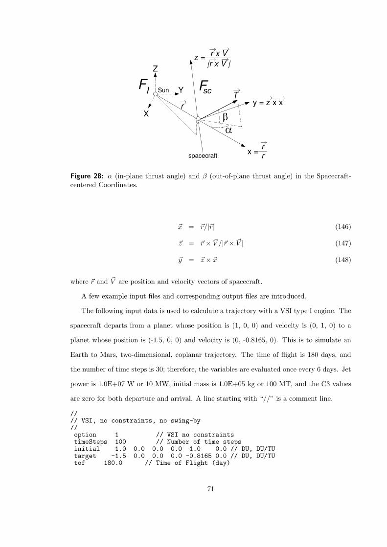
x =
y = z x x
z =
T
X
Y
Z
F I r
Sun
spacecraft r r
r x V |r x V |
F sc
Figure 28: α (in-plane thrust angle) and β (out-of-plane thrust angle) in the Spacecraft-centered Coordinates.
~x = ~r/|~r| (146)
~z = ~r × ~V /|~r × ~V | (147)
~y = ~z × ~x (148)
where ~r and ~V are position and velocity vectors of spacecraft.
A few example input files and corresponding output files are introduced.
The following input data is used to calculate a trajectory with a VSI type I engine. The
spacecraft departs from a planet whose position is (1, 0, 0) and velocity is (0, 1, 0) to a
planet whose position is (-1.5, 0, 0) and velocity is (0, -0.8165, 0). This is to simulate an
Earth to Mars, two-dimensional, coplanar trajectory. The time of flight is 180 days, and
the number of time steps is 30; therefore, the variables are evaluated once every 6 days. Jet
power is 1.0E+07 W or 10 MW, initial mass is 1.0E+05 kg or 100 MT, and the C3 values
are zero for both departure and arrival. A line starting with “//” is a comment line.
//// VSI, no constraints, no swing-by//option 1 // VSI no constraintstimeSteps 100 // Number of time stepsinitial 1.0 0.0 0.0 0.0 1.0 0.0 // DU, DU/TUtarget -1.5 0.0 0.0 0.0 -0.8165 0.0 // DU, DU/TUtof 180.0 // Time of Flight (day)
71
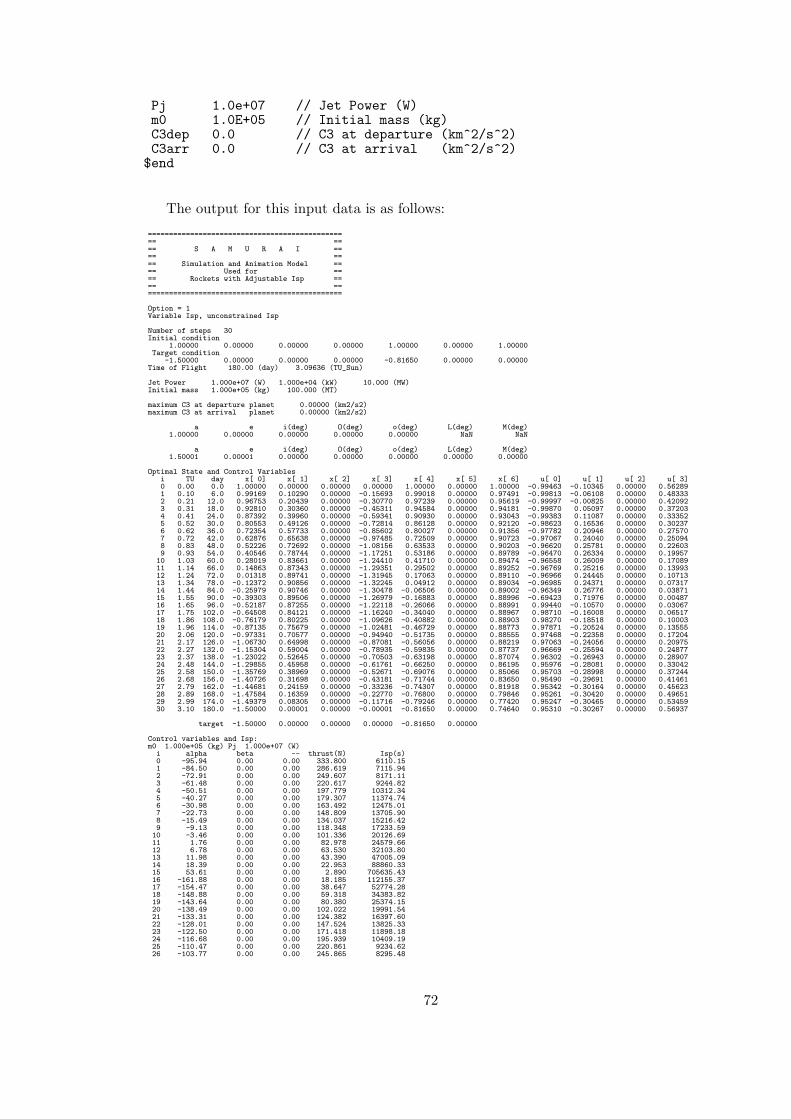
Pj 1.0e+07 // Jet Power (W)m0 1.0E+05 // Initial mass (kg)C3dep 0.0 // C3 at departure (km^2/s^2)C3arr 0.0 // C3 at arrival (km^2/s^2)$end
The output for this input data is as follows:
================================================ ==== S A M U R A I ==== ==== Simulation and Animation Model ==== Used for ==== Rockets with Adjustable Isp ==== ================================================
Option = 1Variable Isp, unconstrained Isp
Number of steps 30Initial condition
1.00000 0.00000 0.00000 0.00000 1.00000 0.00000 1.00000Target condition
-1.50000 0.00000 0.00000 0.00000 -0.81650 0.00000 0.00000Time of Flight 180.00 (day) 3.09636 (TU_Sun)
Jet Power 1.000e+07 (W) 1.000e+04 (kW) 10.000 (MW)Initial mass 1.000e+05 (kg) 100.000 (MT)
maximum C3 at departure planet 0.00000 (km2/s2)maximum C3 at arrival planet 0.00000 (km2/s2)
a e i(deg) O(deg) o(deg) L(deg) M(deg)1.00000 0.00000 0.00000 0.00000 0.00000 NaN NaN
a e i(deg) O(deg) o(deg) L(deg) M(deg)1.50001 0.00001 0.00000 0.00000 0.00000 0.00000 0.00000
Optimal State and Control Variablesi TU day x[ 0] x[ 1] x[ 2] x[ 3] x[ 4] x[ 5] x[ 6] u[ 0] u[ 1] u[ 2] u[ 3]0 0.00 0.0 1.00000 0.00000 0.00000 0.00000 1.00000 0.00000 1.00000 -0.99463 -0.10345 0.00000 0.562891 0.10 6.0 0.99169 0.10290 0.00000 -0.15693 0.99018 0.00000 0.97491 -0.99813 -0.06108 0.00000 0.483332 0.21 12.0 0.96753 0.20439 0.00000 -0.30770 0.97239 0.00000 0.95619 -0.99997 -0.00825 0.00000 0.420923 0.31 18.0 0.92810 0.30360 0.00000 -0.45311 0.94584 0.00000 0.94181 -0.99870 0.05097 0.00000 0.372034 0.41 24.0 0.87392 0.39960 0.00000 -0.59341 0.90930 0.00000 0.93043 -0.99383 0.11087 0.00000 0.333525 0.52 30.0 0.80553 0.49126 0.00000 -0.72814 0.86128 0.00000 0.92120 -0.98623 0.16536 0.00000 0.302376 0.62 36.0 0.72354 0.57733 0.00000 -0.85602 0.80027 0.00000 0.91356 -0.97782 0.20946 0.00000 0.275707 0.72 42.0 0.62876 0.65638 0.00000 -0.97485 0.72509 0.00000 0.90723 -0.97067 0.24040 0.00000 0.250948 0.83 48.0 0.52226 0.72692 0.00000 -1.08156 0.63533 0.00000 0.90203 -0.96620 0.25781 0.00000 0.226039 0.93 54.0 0.40546 0.78744 0.00000 -1.17251 0.53186 0.00000 0.89789 -0.96470 0.26334 0.00000 0.1995710 1.03 60.0 0.28019 0.83661 0.00000 -1.24410 0.41710 0.00000 0.89474 -0.96558 0.26009 0.00000 0.1708911 1.14 66.0 0.14863 0.87343 0.00000 -1.29351 0.29502 0.00000 0.89252 -0.96769 0.25216 0.00000 0.1399312 1.24 72.0 0.01318 0.89741 0.00000 -1.31945 0.17063 0.00000 0.89110 -0.96966 0.24445 0.00000 0.1071313 1.34 78.0 -0.12372 0.90856 0.00000 -1.32245 0.04912 0.00000 0.89034 -0.96985 0.24371 0.00000 0.0731714 1.44 84.0 -0.25979 0.90746 0.00000 -1.30478 -0.06506 0.00000 0.89002 -0.96349 0.26776 0.00000 0.0387115 1.55 90.0 -0.39303 0.89506 0.00000 -1.26979 -0.16883 0.00000 0.88996 -0.69423 0.71976 0.00000 0.0048716 1.65 96.0 -0.52187 0.87255 0.00000 -1.22118 -0.26066 0.00000 0.88991 0.99440 -0.10570 0.00000 0.0306717 1.75 102.0 -0.64508 0.84121 0.00000 -1.16240 -0.34040 0.00000 0.88967 0.98710 -0.16008 0.00000 0.0651718 1.86 108.0 -0.76179 0.80225 0.00000 -1.09626 -0.40882 0.00000 0.88903 0.98270 -0.18518 0.00000 0.1000319 1.96 114.0 -0.87135 0.75679 0.00000 -1.02481 -0.46729 0.00000 0.88773 0.97871 -0.20524 0.00000 0.1355520 2.06 120.0 -0.97331 0.70577 0.00000 -0.94940 -0.51735 0.00000 0.88555 0.97468 -0.22358 0.00000 0.1720421 2.17 126.0 -1.06730 0.64998 0.00000 -0.87081 -0.56056 0.00000 0.88219 0.97063 -0.24056 0.00000 0.2097522 2.27 132.0 -1.15304 0.59004 0.00000 -0.78935 -0.59835 0.00000 0.87737 0.96669 -0.25594 0.00000 0.2487723 2.37 138.0 -1.23022 0.52645 0.00000 -0.70503 -0.63198 0.00000 0.87074 0.96302 -0.26943 0.00000 0.2890724 2.48 144.0 -1.29855 0.45958 0.00000 -0.61761 -0.66250 0.00000 0.86195 0.95976 -0.28081 0.00000 0.3304225 2.58 150.0 -1.35769 0.38969 0.00000 -0.52671 -0.69076 0.00000 0.85066 0.95703 -0.28998 0.00000 0.3724426 2.68 156.0 -1.40726 0.31698 0.00000 -0.43181 -0.71744 0.00000 0.83650 0.95490 -0.29691 0.00000 0.4146127 2.79 162.0 -1.44681 0.24159 0.00000 -0.33236 -0.74307 0.00000 0.81918 0.95342 -0.30164 0.00000 0.4562328 2.89 168.0 -1.47584 0.16359 0.00000 -0.22770 -0.76800 0.00000 0.79846 0.95261 -0.30420 0.00000 0.4965129 2.99 174.0 -1.49379 0.08305 0.00000 -0.11716 -0.79246 0.00000 0.77420 0.95247 -0.30465 0.00000 0.5345930 3.10 180.0 -1.50000 0.00001 0.00000 -0.00001 -0.81650 0.00000 0.74640 0.95310 -0.30267 0.00000 0.56937
target -1.50000 0.00000 0.00000 0.00000 -0.81650 0.00000
Control variables and Isp:m0 1.000e+05 (kg) Pj 1.000e+07 (W)
i alpha beta -- thrust(N) Isp(s)0 -95.94 0.00 0.00 333.800 6110.151 -84.50 0.00 0.00 286.619 7115.942 -72.91 0.00 0.00 249.607 8171.113 -61.48 0.00 0.00 220.617 9244.824 -50.51 0.00 0.00 197.779 10312.345 -40.27 0.00 0.00 179.307 11374.746 -30.98 0.00 0.00 163.492 12475.017 -22.73 0.00 0.00 148.809 13705.908 -15.49 0.00 0.00 134.037 15216.429 -9.13 0.00 0.00 118.348 17233.59
10 -3.46 0.00 0.00 101.336 20126.6911 1.76 0.00 0.00 82.978 24579.6612 6.78 0.00 0.00 63.530 32103.8013 11.98 0.00 0.00 43.390 47005.0914 18.39 0.00 0.00 22.953 88860.3315 53.61 0.00 0.00 2.890 705635.4316 -161.88 0.00 0.00 18.185 112155.3717 -154.47 0.00 0.00 38.647 52774.2818 -148.88 0.00 0.00 59.318 34383.8219 -143.64 0.00 0.00 80.380 25374.1520 -138.49 0.00 0.00 102.022 19991.5421 -133.31 0.00 0.00 124.382 16397.6022 -128.01 0.00 0.00 147.524 13825.3323 -122.50 0.00 0.00 171.418 11898.1824 -116.68 0.00 0.00 195.939 10409.1925 -110.47 0.00 0.00 220.861 9234.6226 -103.77 0.00 0.00 245.865 8295.48
72
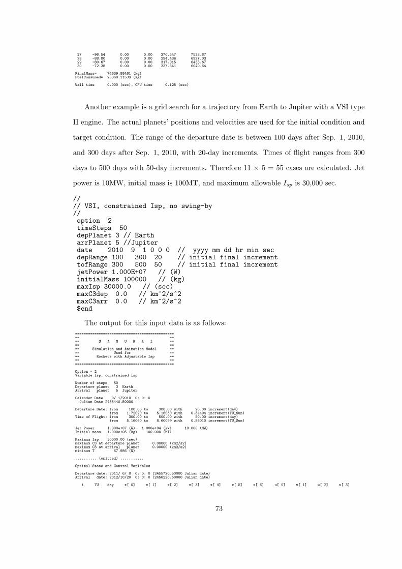
27 -96.54 0.00 0.00 270.547 7538.6728 -88.80 0.00 0.00 294.436 6927.0329 -80.67 0.00 0.00 317.015 6433.6730 -72.38 0.00 0.00 337.641 6040.64
FinalMass= 74639.88461 (kg)FuelConsumed= 25360.11539 (kg)
Wall time 0.000 (sec), CPU time 0.125 (sec)
Another example is a grid search for a trajectory from Earth to Jupiter with a VSI type
II engine. The actual planets’ positions and velocities are used for the initial condition and
target condition. The range of the departure date is between 100 days after Sep. 1, 2010,
and 300 days after Sep. 1, 2010, with 20-day increments. Times of flight ranges from 300
days to 500 days with 50-day increments. Therefore 11 × 5 = 55 cases are calculated. Jet
power is 10MW, initial mass is 100MT, and maximum allowable Isp is 30,000 sec.
//// VSI, constrained Isp, no swing-by//option 2timeSteps 50depPlanet 3 // EartharrPlanet 5 //Jupiterdate 2010 9 1 0 0 0 // yyyy mm dd hr min secdepRange 100 300 20 // initial final incrementtofRange 300 500 50 // initial final incrementjetPower 1.000E+07 // (W)initialMass 100000 // (kg)maxIsp 30000.0 // (sec)maxC3dep 0.0 // km^2/s^2maxC3arr 0.0 // km^2/s^2$end
The output for this input data is as follows:
================================================ ==== S A M U R A I ==== ==== Simulation and Animation Model ==== Used for ==== Rockets with Adjustable Isp ==== ================================================
Option = 2Variable Isp, constrained Isp
Number of steps 50Departure planet 3 EarthArrival planet 5 Jupiter
Calender Date 9/ 1/2010 0: 0: 0Julian Date 2455440.50000
Departure Date: from 100.00 to 300.00 with 20.00 increment(day)from 1.72020 to 5.16060 with 0.34404 increment(TU_Sun)
Time of Flight: from 300.00 to 500.00 with 50.00 increment(day)from 5.16060 to 8.60099 with 0.86010 increment(TU_Sun)
Jet Power 1.000e+07 (W) 1.000e+04 (kW) 10.000 (MW)Initial mass 1.000e+05 (kg) 100.000 (MT)
Maximum Isp 30000.00 (sec)maximum C3 at departure planet 0.00000 (km2/s2)maximum C3 at arrival planet 0.00000 (km2/s2)mininum T 67.986 (N)
........... (omitted) ...........
Optimal State and Control Variables
Departure date: 2011/ 6/ 8 0: 0: 0 (2455720.50000 Julian date)Arrival date: 2012/10/20 0: 0: 0 (2456220.50000 Julian date)
i TU day x[ 0] x[ 1] x[ 2] x[ 3] x[ 4] x[ 5] x[ 6] u[ 0] u[ 1] u[ 2] u[ 3]
73
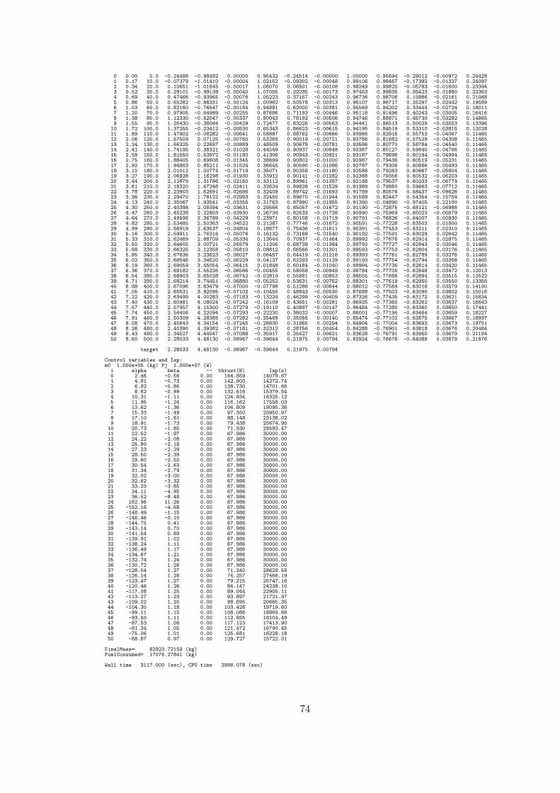
0 0.00 0.0 -0.24488 -0.98482 0.00000 0.95432 -0.24514 -0.00000 1.00000 0.95694 -0.29012 -0.00972 0.244281 0.17 10.0 -0.07379 -1.01410 -0.00004 1.02152 -0.09302 -0.00048 0.99106 0.98467 -0.17392 -0.01327 0.240972 0.34 20.0 0.10651 -1.01645 -0.00017 1.06070 0.06501 -0.00108 0.98249 0.99820 -0.05783 -0.01600 0.233943 0.52 30.0 0.29101 -0.99138 -0.00040 1.07055 0.22235 -0.00173 0.97453 0.99835 0.05423 -0.01880 0.223634 0.69 40.0 0.47466 -0.93965 -0.00076 1.05223 0.37157 -0.00243 0.96736 0.98706 0.15886 -0.02161 0.210685 0.86 50.0 0.65282 -0.86331 -0.00124 1.00962 0.50578 -0.00313 0.96107 0.96717 0.25297 -0.02442 0.195896 1.03 60.0 0.82180 -0.76547 -0.00184 0.94881 0.62000 -0.00381 0.95569 0.94202 0.33444 -0.02724 0.180117 1.20 70.0 0.97905 -0.64989 -0.00255 0.87686 0.71193 -0.00446 0.95118 0.91496 0.40243 -0.03005 0.164168 1.38 80.0 1.12330 -0.52047 -0.00337 0.80043 0.78192 -0.00506 0.94746 0.88871 0.45730 -0.03282 0.148659 1.55 90.0 1.25430 -0.38084 -0.00429 0.72477 0.83226 -0.00563 0.94441 0.86513 0.50029 -0.03553 0.1339610 1.72 100.0 1.37255 -0.23412 -0.00530 0.65343 0.86623 -0.00615 0.94195 0.84519 0.53310 -0.03815 0.1202811 1.89 110.0 1.47902 -0.08282 -0.00641 0.58887 0.88762 -0.00666 0.93986 0.82916 0.55753 -0.04067 0.1146512 2.06 120.0 1.57509 0.07125 -0.00760 0.53268 0.90019 -0.00721 0.93786 0.81682 0.57529 -0.04308 0.1146513 2.24 130.0 1.66225 0.22687 -0.00889 0.48509 0.90678 -0.00781 0.93586 0.80770 0.58784 -0.04540 0.1146514 2.41 140.0 1.74195 0.38321 -0.01028 0.44549 0.90937 -0.00848 0.93387 0.80127 0.59640 -0.04766 0.1146515 2.58 150.0 1.81550 0.53972 -0.01180 0.41306 0.90943 -0.00921 0.93187 0.79698 0.60194 -0.04994 0.1146516 2.75 160.0 1.88405 0.69608 -0.01345 0.38699 0.90802 -0.01000 0.92987 0.79436 0.60519 -0.05231 0.1146517 2.92 170.0 1.94863 0.85211 -0.01524 0.36645 0.90590 -0.01086 0.92787 0.79306 0.60666 -0.05493 0.1146518 3.10 180.0 2.01012 1.00774 -0.01719 0.35071 0.90358 -0.01180 0.92588 0.79283 0.60667 -0.05804 0.1146519 3.27 190.0 2.06928 1.16298 -0.01930 0.33912 0.90141 -0.01282 0.92388 0.79356 0.60532 -0.06203 0.1146520 3.44 200.0 2.12679 1.31786 -0.02160 0.33112 0.89961 -0.01397 0.92188 0.79537 0.60233 -0.06774 0.1146521 3.61 210.0 2.18320 1.47248 -0.02411 0.32624 0.89828 -0.01529 0.91989 0.79880 0.59663 -0.07712 0.1146522 3.78 220.0 2.23903 1.62691 -0.02686 0.32409 0.89742 -0.01693 0.91789 0.80576 0.58437 -0.09628 0.1146523 3.96 230.0 2.29470 1.78122 -0.02993 0.32450 0.89670 -0.01944 0.91589 0.82447 0.54354 -0.15754 0.1146524 4.13 240.0 2.35067 1.93541 -0.03355 0.31763 0.87990 -0.01855 0.91390 -0.04890 -0.97405 0.22100 0.1146525 4.30 250.0 2.40398 2.08394 -0.03631 0.29566 0.85057 -0.01672 0.91190 -0.72875 -0.68121 -0.06988 0.1146526 4.47 260.0 2.45238 2.22803 -0.03930 0.26734 0.82533 -0.01738 0.90990 -0.75969 -0.65023 -0.00879 0.1146527 4.64 270.0 2.49596 2.36789 -0.04229 0.23971 0.80108 -0.01719 0.90791 -0.76826 -0.64007 0.00930 0.1146528 4.82 280.0 2.53485 2.50363 -0.04522 0.21287 0.77746 -0.01672 0.90591 -0.77228 -0.63503 0.01800 0.1146529 4.99 290.0 2.56919 2.63537 -0.04804 0.18677 0.75436 -0.01611 0.90391 -0.77453 -0.63211 0.02310 0.1146530 5.16 300.0 2.59911 2.76316 -0.05076 0.16132 0.73168 -0.01540 0.90192 -0.77591 -0.63029 0.02642 0.1146531 5.33 310.0 2.62469 2.88709 -0.05334 0.13644 0.70937 -0.01464 0.89992 -0.77676 -0.62914 0.02875 0.1146532 5.50 320.0 2.64605 3.00721 -0.05579 0.11206 0.68738 -0.01384 0.89792 -0.77727 -0.62843 0.03046 0.1146533 5.68 330.0 2.66325 3.12358 -0.05810 0.08812 0.66566 -0.01301 0.89593 -0.77753 -0.62804 0.03176 0.1146534 5.85 340.0 2.67636 3.23623 -0.06027 0.06457 0.64419 -0.01216 0.89393 -0.77761 -0.62789 0.03276 0.1146535 6.02 350.0 2.68546 3.34520 -0.06229 0.04137 0.62293 -0.01129 0.89193 -0.77754 -0.62794 0.03356 0.1146536 6.19 360.0 2.69059 3.45054 -0.06415 0.01848 0.60184 -0.01040 0.88994 -0.77735 -0.62814 0.03420 0.1146537 6.36 370.0 2.69182 3.55226 -0.06586 -0.00455 0.58058 -0.00949 0.88784 -0.77705 -0.62848 0.03472 0.1201338 6.54 380.0 2.68903 3.65028 -0.06742 -0.02814 0.55881 -0.00853 0.88555 -0.77666 -0.62894 0.03515 0.1252239 6.71 390.0 2.68214 3.74451 -0.06880 -0.05252 0.53631 -0.00752 0.88301 -0.77619 -0.62950 0.03550 0.1335840 6.88 400.0 2.67096 3.83479 -0.07000 -0.07798 0.51286 -0.00644 0.88012 -0.77564 -0.63016 0.03579 0.1419041 7.05 410.0 2.65531 3.92095 -0.07102 -0.10455 0.48843 -0.00530 0.87688 -0.77503 -0.63090 0.03602 0.1501642 7.22 420.0 2.63499 4.00283 -0.07183 -0.13224 0.46299 -0.00409 0.87326 -0.77435 -0.63172 0.03621 0.1583443 7.40 430.0 2.60981 4.08024 -0.07242 -0.16109 0.43651 -0.00281 0.86925 -0.77360 -0.63262 0.03637 0.1664344 7.57 440.0 2.57957 4.15300 -0.07279 -0.19110 0.40897 -0.00147 0.86484 -0.77280 -0.63360 0.03650 0.1744145 7.74 450.0 2.54406 4.22094 -0.07293 -0.22230 0.38032 -0.00007 0.86001 -0.77194 -0.63464 0.03659 0.1822746 7.91 460.0 2.50309 4.28385 -0.07282 -0.25469 0.35056 0.00140 0.85474 -0.77102 -0.63575 0.03667 0.1899747 8.08 470.0 2.45643 4.34154 -0.07245 -0.28830 0.31965 0.00294 0.84904 -0.77004 -0.63693 0.03673 0.1975148 8.26 480.0 2.40390 4.39382 -0.07181 -0.32312 0.28756 0.00454 0.84288 -0.76901 -0.63818 0.03676 0.2048449 8.43 490.0 2.34527 4.44047 -0.07088 -0.35917 0.25427 0.00621 0.83628 -0.76791 -0.63950 0.03679 0.2119450 8.60 500.0 2.28033 4.48130 -0.06967 -0.39644 0.21975 0.00794 0.82924 -0.76676 -0.64088 0.03679 0.21876
target 2.28033 4.48130 -0.06967 -0.39644 0.21975 0.00794
Control variables and Isp:m0 1.000e+05 (kg) Pj 1.000e+07 (W)
i alpha beta -- thrust(N) Isp(s)0 2.46 -0.56 0.00 144.859 14079.671 4.81 -0.73 0.00 142.900 14272.742 6.82 -0.86 0.00 138.730 14701.663 8.62 -0.99 0.00 132.616 15379.544 10.31 -1.11 0.00 124.934 16325.125 11.95 -1.24 0.00 116.162 17558.036 13.62 -1.36 0.00 106.809 19095.387 15.33 -1.49 0.00 97.350 20950.978 17.10 -1.61 0.00 88.148 23138.029 18.91 -1.73 0.00 79.438 25674.95
10 20.73 -1.85 0.00 71.330 28593.4711 22.52 -1.97 0.00 67.986 30000.0012 24.22 -2.08 0.00 67.986 30000.0013 25.80 -2.18 0.00 67.986 30000.0014 27.23 -2.29 0.00 67.986 30000.0015 28.50 -2.39 0.00 67.986 30000.0016 29.60 -2.50 0.00 67.986 30000.0017 30.54 -2.63 0.00 67.986 30000.0018 31.34 -2.79 0.00 67.986 30000.0019 32.02 -3.00 0.00 67.986 30000.0020 32.62 -3.32 0.00 67.986 30000.0021 33.23 -3.85 0.00 67.986 30000.0022 34.11 -4.95 0.00 67.986 30000.0023 36.52 -8.48 0.00 67.986 30000.0024 162.96 11.26 0.00 67.986 30000.0025 -152.16 -4.68 0.00 67.986 30000.0026 -148.49 -1.15 0.00 67.986 30000.0027 -146.46 -0.10 0.00 67.986 30000.0028 -144.75 0.41 0.00 67.986 30000.0029 -143.14 0.70 0.00 67.986 30000.0030 -141.54 0.89 0.00 67.986 30000.0031 -139.91 1.02 0.00 67.986 30000.0032 -138.24 1.11 0.00 67.986 30000.0033 -136.49 1.17 0.00 67.986 30000.0034 -134.67 1.21 0.00 67.986 30000.0035 -132.74 1.24 0.00 67.986 30000.0036 -130.72 1.26 0.00 67.986 30000.0037 -128.54 1.27 0.00 71.240 28629.5838 -126.14 1.28 0.00 74.257 27466.1939 -123.47 1.27 0.00 79.215 25747.1640 -120.46 1.26 0.00 84.147 24238.1041 -117.08 1.25 0.00 89.044 22905.1142 -113.27 1.23 0.00 93.897 21721.3743 -109.02 1.20 0.00 98.695 20665.3544 -104.30 1.18 0.00 103.428 19719.6045 -99.11 1.15 0.00 108.086 18869.8846 -93.50 1.11 0.00 112.655 18104.4947 -87.53 1.08 0.00 117.123 17413.9048 -81.34 1.05 0.00 121.472 16790.4549 -75.06 1.01 0.00 125.681 16228.1850 -68.87 0.97 0.00 129.727 15722.01
FinalMass= 82923.72159 (kg)FuelConsumed= 17076.27841 (kg)
Wall time 3117.000 (sec), CPU time 2998.078 (sec)
74
The precise explanation of input data is in Appendix D.
6.5 Validation and Verification
When a new computer application is created, validation is necessary to check if the applica-
tion works properly. In order to validate SAMURAI, several analyses have been performed
and the results with SAMURAI are compared to the results with other existing reliable
interplanetary trajectory calculation programs.
There are no applications to calculate general VSI trajectories. Therefore, validation for
CSI engines and high thrust engines are performed. IPREP is used to compare the results
for high thrust, and ChebyTOP is used for CSI trajectories.
6.5.1 Validation of High Thrust with IPREP
IPREP (Interplanetary PREProcessor) is a rapid grid-search optimizer on launch and arrival
windows, minimum ∆V or mass optimization created by Martin Marietta Astronautics.
IPREP is widely used to estimate ∆V for high thrust trajectories.
To compare the results with SAMURAI and the results with IPREP, transfer trajectories
are calculated from Earth to Venus, Mars, and Jupiter. Times of flight are set to 200 days
for Venus transfer, 360 days for Mars transfer, and 500 days for Jupiter transfer. Twelve
departure dates are considered: the first day of the month in the year 2000.
Figs. 29 to 31 show the ∆V requirements (at departure and arrival, and total) calculated
with SAMURAI and IPREP. They show that the results obtained by SAMURAI match well
with the results obtained by IPREP.
6.5.2 Validation of CSI with ChebyTOP
ChebyTOP (Chebyshev Trajectory Optimization Program) is an analysis tool that enables
the user to conduct rapidly the parametric analysis and optimization of interplanetary
missions employing electrically propelled spacecraft developed by Boeing.
To compare the results with SAMURAI and the results with ChebyTOP, transfer tra-
jectories from Earth to Mars are analyzed for CSI type I and type II engines. The following
75
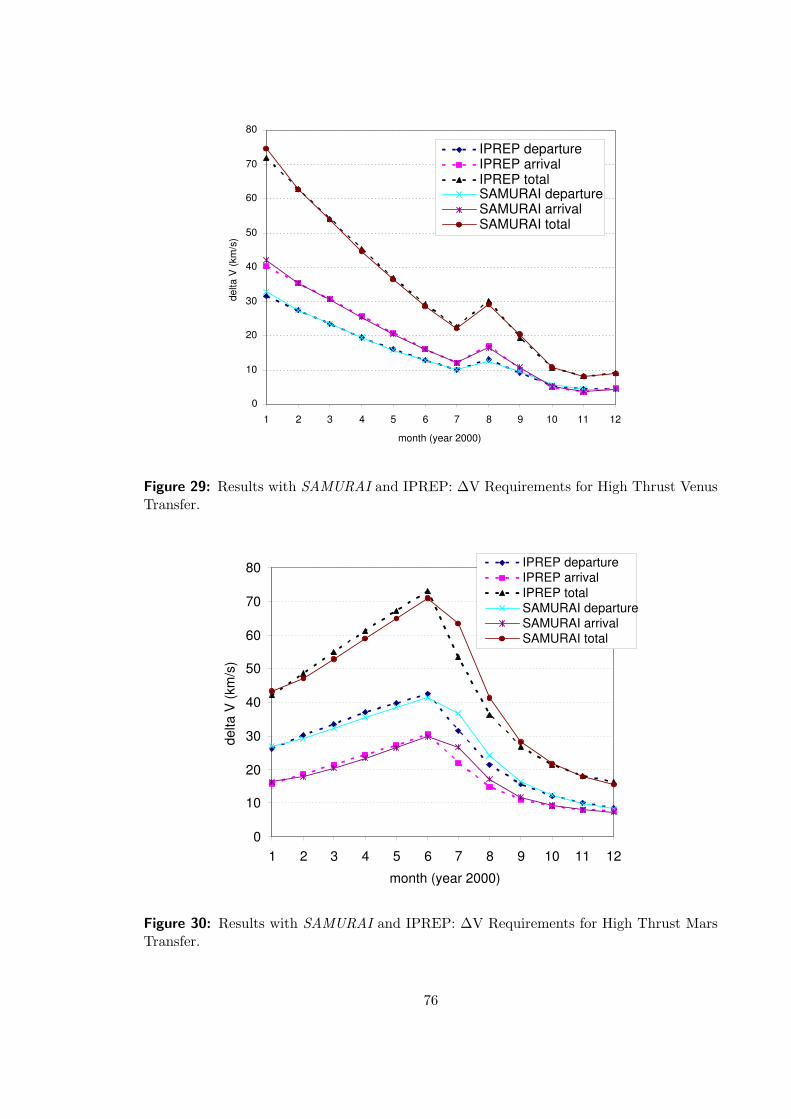
0
10
20
30
40
50
60
70
80
1 2 3 4 5 6 7 8 9 10 11 12
month (year 2000)
delta
V (k
m/s
)
IPREP departure IPREP arrival IPREP total SAMURAI departure SAMURAI arrival SAMURAI total
Figure 29: Results with SAMURAI and IPREP: ∆V Requirements for High Thrust VenusTransfer.
0
10
20
30
40
50
60
70
80
1 2 3 4 5 6 7 8 9 10 11 12
month (year 2000)
delta
V (k
m/s
)
IPREP departure IPREP arrival IPREP total SAMURAI departure SAMURAI arrival SAMURAI total
Figure 30: Results with SAMURAI and IPREP: ∆V Requirements for High Thrust MarsTransfer.
76
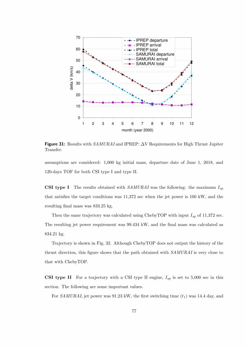
0
10
20
30
40
50
60
70
1 2 3 4 5 6 7 8 9 10 11 12
month (year 2000)
delta
V (k
m/s
)
IPREP departure IPREP arrival IPREP total SAMURAI departure SAMURAI arrival SAMURAI total
Figure 31: Results with SAMURAI and IPREP: ∆V Requirements for High Thrust JupiterTransfer.
assumptions are considered: 1,000 kg initial mass, departure date of June 1, 2018, and
120-days TOF for both CSI type I and type II.
CSI type I The results obtained with SAMURAI was the following: the maximum Isp
that satisfies the target conditions was 11,372 sec when the jet power is 100 kW, and the
resulting final mass was 833.25 kg.
Then the same trajectory was calculated using ChebyTOP with input Isp of 11,372 sec.
The resulting jet power requirement was 99.434 kW, and the final mass was calculated as
834.21 kg.
Trajectory is shown in Fig. 32. Although ChebyTOP does not output the history of the
thrust direction, this figure shows that the path obtained with SAMURAI is very close to
that with ChebyTOP.
CSI type II For a trajectory with a CSI type II engine, Isp is set to 5,000 sec in this
section. The following are some important values.
For SAMURAI, jet power was 91.23 kW, the first switching time (t1) was 14.4 day, and
77
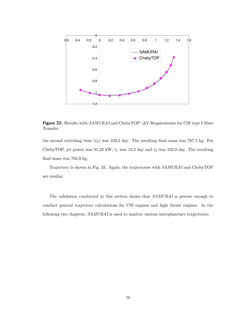
-1.2
-1
-0.8
-0.6
-0.4
-0.2
0 -0.6 -0.4 -0.2 0 0.2 0.4 0.6 0.8 1 1.2 1.4 1.6
SAMURAI ChebyTOP
Figure 32: Results with SAMURAI and ChebyTOP: ∆V Requirements for CSI type I MarsTransfer.
the second switching time (t2) was 103.2 day. The resulting final mass was 787.5 kg. For
ChebyTOP, jet power was 91.23 kW, t1 was 13.3 day and t2 was 102.0 day. The resulting
final mass was 794.9 kg.
Trajectory is shown in Fig. 33. Again, the trajectories with SAMURAI and ChebyTOP
are similar.
The validation conducted in this section shows that SAMURAI is precise enough to
conduct general trajectory calculations for CSI engines and high thrust engines. In the
following two chapters, SAMURAI is used to analyze various interplanetary trajectories.
78
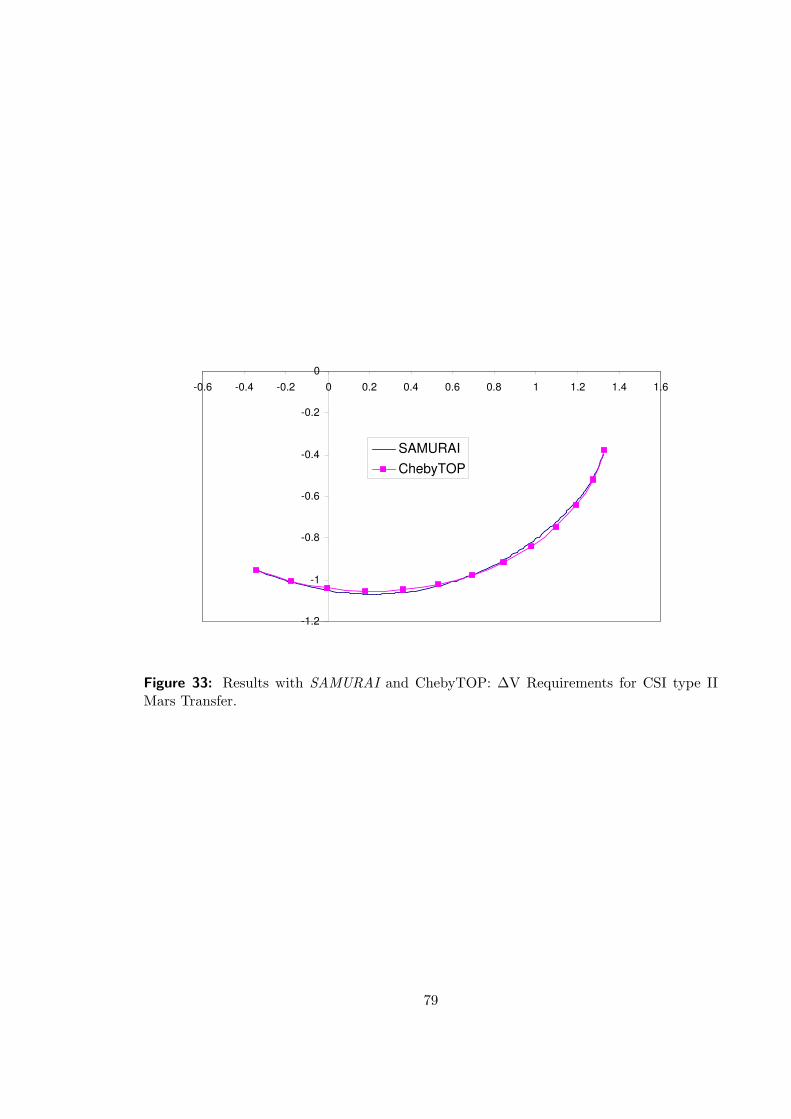
-1.2
-1
-0.8
-0.6
-0.4
-0.2
0 -0.6 -0.4 -0.2 0 0.2 0.4 0.6 0.8 1 1.2 1.4 1.6
SAMURAI ChebyTOP
Figure 33: Results with SAMURAI and ChebyTOP: ∆V Requirements for CSI type IIMars Transfer.
79
CHAPTER VII
PRELIMINARY RESULTS: PROOF OF CONCEPT
One of the objectives of this research is to compare different types of engines and discuss
their advantages and disadvantages. In this research comparison is performed by calculating
the fuel consumption of each engine for the same trajectory. The trajectories should have
the same initial condition, the same target condition, and the same time of flight. The
problem should be made as simple as possible so that the comparison of these engines
clearly states the advantages or disadvantages of each engine.
In this chapter, a large database is generated using SAMURAI. Transfer orbits from
Earth that circularizes around the Sun to other planets that circularize around the Sun
are calculated for five different engines(VSI type I and II, CSI type I and II, and high
thrust). The fuel consumption for each engine is calculated and compared against the
results obtained for each.
7.1 Problem Description
The minimum fuel transfer trajectory for each of five engines is calculated. The planets are
assumed to be orbiting around the Sun in a circular orbit (zero eccentricity), and these orbits
are further assumed to be coplanar (zero inclination). This allows for a two-dimensional
transfer orbit to be assumed.
Table 4 shows some orbital data for planets. The eccentricity is less than 0.1 and the
inclination is less than a few percents except Mercury and Pluto. The Earth and the four
destination planets considered in this chapter can be thought to be circular and coplanar.
Therefore, considering the orbits of these planets two-dimensional and circular is a good
approximation to the actual orbits.
The spacecraft is assumed to depart from Earth at a position of (x, y) = (1.0, 0.0) and
a velocity of (u, v) = (0.0, 1.0). C3’s at departure and arrival are assumed to be zero for all
80
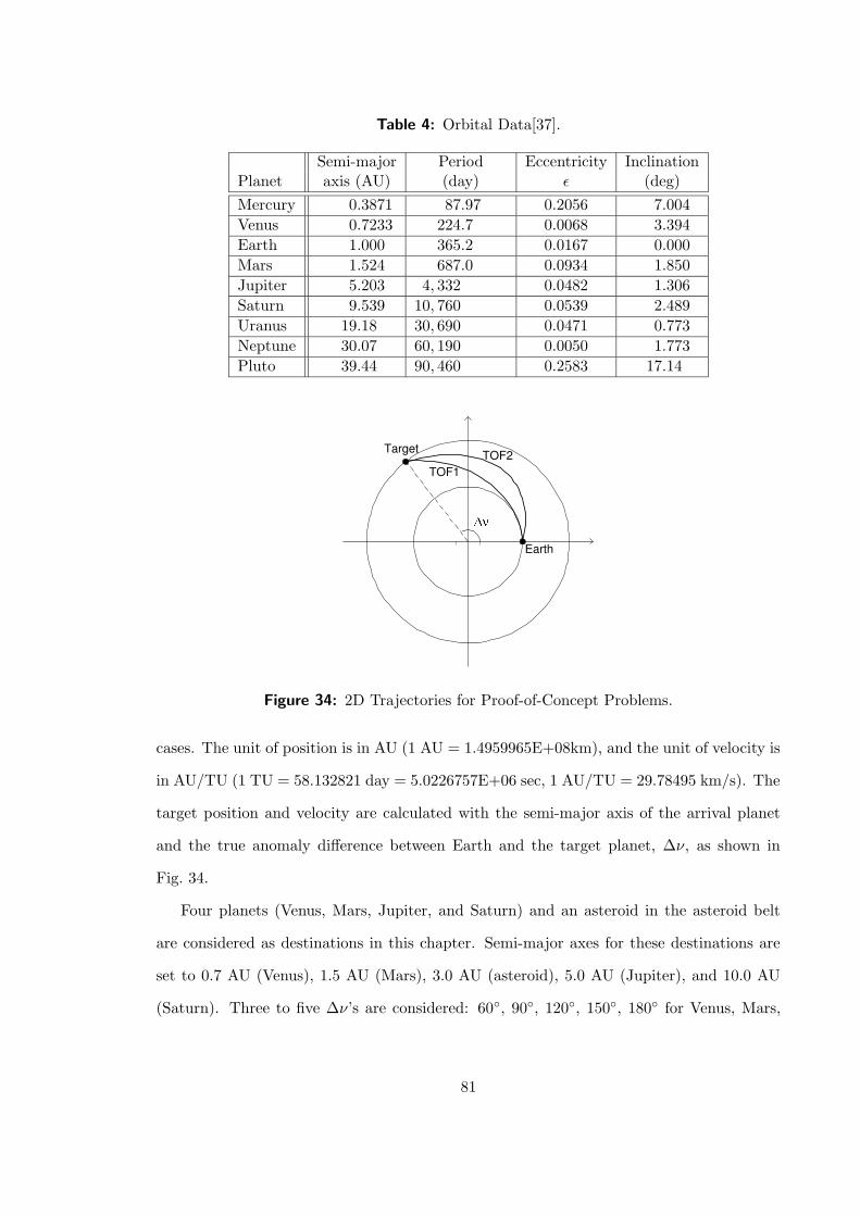
Table 4: Orbital Data[37].
Semi-major Period Eccentricity InclinationPlanet axis (AU) (day) ε (deg)
Mercury 0.3871 87.97 0.2056 7.004
Venus 0.7233 224.7 0.0068 3.394
Earth 1.000 365.2 0.0167 0.000
Mars 1.524 687.0 0.0934 1.850
Jupiter 5.203 4, 332 0.0482 1.306
Saturn 9.539 10, 760 0.0539 2.489
Uranus 19.18 30, 690 0.0471 0.773
Neptune 30.07 60, 190 0.0050 1.773
Pluto 39.44 90, 460 0.2583 17.14
Earth
Target
TOF1 TOF2
Figure 34: 2D Trajectories for Proof-of-Concept Problems.
cases. The unit of position is in AU (1 AU = 1.4959965E+08km), and the unit of velocity is
in AU/TU (1 TU = 58.132821 day = 5.0226757E+06 sec, 1 AU/TU = 29.78495 km/s). The
target position and velocity are calculated with the semi-major axis of the arrival planet
and the true anomaly difference between Earth and the target planet, ∆ν, as shown in
Fig. 34.
Four planets (Venus, Mars, Jupiter, and Saturn) and an asteroid in the asteroid belt
are considered as destinations in this chapter. Semi-major axes for these destinations are
set to 0.7 AU (Venus), 1.5 AU (Mars), 3.0 AU (asteroid), 5.0 AU (Jupiter), and 10.0 AU
(Saturn). Three to five ∆ν’s are considered: 60, 90, 120, 150, 180 for Venus, Mars,
81
and the asteroid, 90, 120, 150, 180 for Jupiter, and 120, 150, 180 for Saturn.
The velocity of a spacecraft on a circular orbit with radius r is expressed as√
µ/r where
the gravitational parameter µ in the canonical units is 1 AU3/TU2. Hence, if Mars is chosen
as the target planet and ∆ν = 120 is used, the target condition is
position (x, y) = (1.5 cos 120, 1.5 sin 120) = (−0.750, 1.299),
velocity (u, v) = (−√
1
1.5sin 120,
√
1
1.5cos 120) = (−0.707,−0.408).
Three levels of the jet power (10, 20, and 30MW) are considered for all destinations,
and the initial mass is set to 1.0E+05 kg (100MT) for all cases.
For each target condition and jet power, the trajectory for several values of time of
flight are calculated. The range for the time of flight for each destination is selected so
that it includes the time of flight that minimizes the fuel consumption for high thrust. For
example, the time of flight for a Hohmann transfer from Earth to Mars is 4.454 TU, so the
range of time of flight for Earth → Mars trajectories with ∆ν = 180 is chosen between 3.0
TU and 5.0 TU.
For VSI type II (bounded Isp case), the maximum allowable Isp is set to 30,000 seconds.
The Isp is determined by the exhaust velocity of the engine. An Isp of 30,000 seconds is
appropriate with current or near-future technology [22].
For CSI type I, the minimum required thrust level that enables the spacecraft to reach
the target is calculated. For example, higher thrust (and hence lower Isp) is required for fast
transfer and therefore higher fuel consumption is expected for this case. On the other hand,
when the transfer time is very long, less thrust (and higher Isp) is required and therefore
small amount of fuel may be needed.
For CSI type II (bang-off-bang case) the Isp level is set to 5,000 seconds, and he Isp for
high thrust is set to 450 seconds.
7.2 Numerical Accuracy
Before calculating the transfer trajectories, the numerical accuracy is investigated to deter-
mine the tolerance and number of time steps required. Input values for these parameters
are determined based on the discussion in the remaining sections of this paper.
82
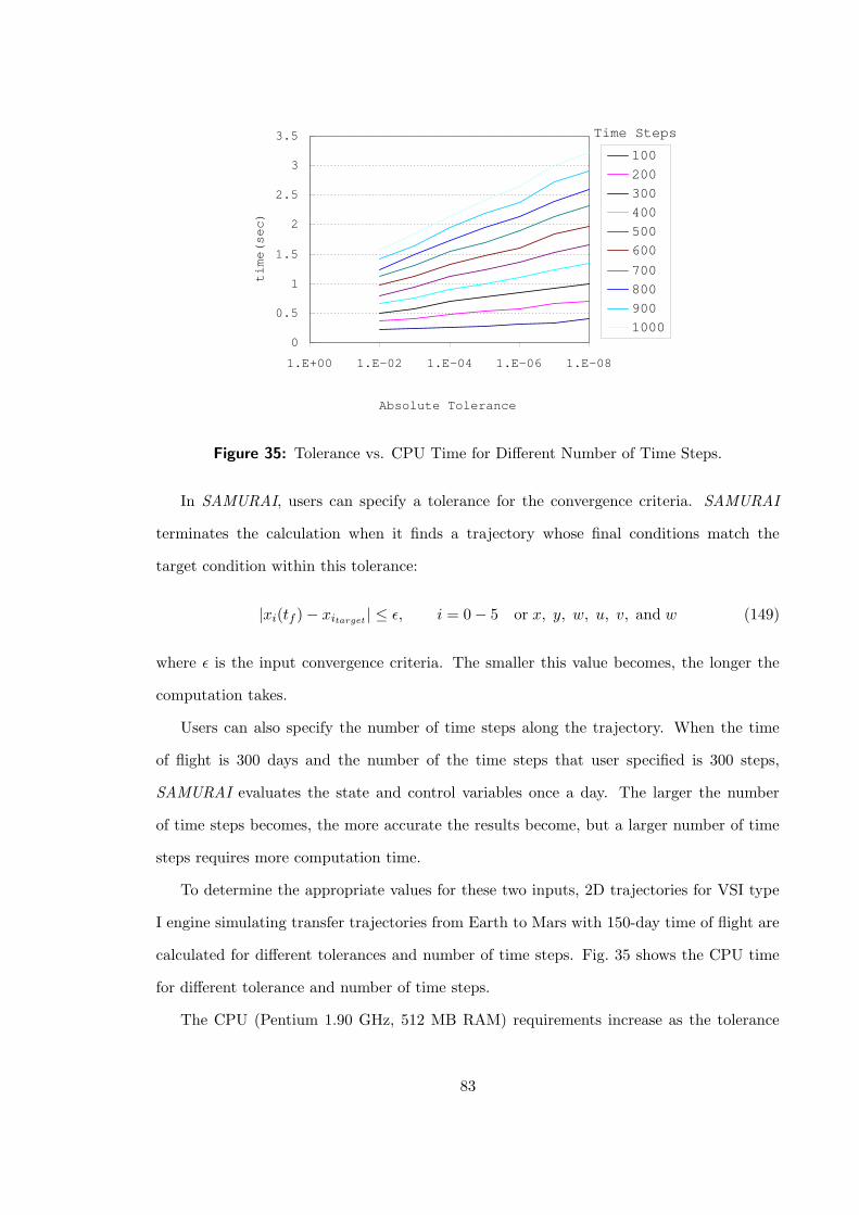
Time Steps
0
0.5
1
1.5
2
2.5
3
3.5
1.E-08 1.E-06 1.E-04 1.E-02 1.E+00
Absolute Tolerance
time(sec)
100
200
300
400
500
600
700
800
900
1000
Figure 35: Tolerance vs. CPU Time for Different Number of Time Steps.
In SAMURAI, users can specify a tolerance for the convergence criteria. SAMURAI
terminates the calculation when it finds a trajectory whose final conditions match the
target condition within this tolerance:
|xi(tf ) − xitarget | ≤ ε, i = 0 − 5 or x, y, w, u, v, and w (149)
where ε is the input convergence criteria. The smaller this value becomes, the longer the
computation takes.
Users can also specify the number of time steps along the trajectory. When the time
of flight is 300 days and the number of the time steps that user specified is 300 steps,
SAMURAI evaluates the state and control variables once a day. The larger the number
of time steps becomes, the more accurate the results become, but a larger number of time
steps requires more computation time.
To determine the appropriate values for these two inputs, 2D trajectories for VSI type
I engine simulating transfer trajectories from Earth to Mars with 150-day time of flight are
calculated for different tolerances and number of time steps. Fig. 35 shows the CPU time
for different tolerance and number of time steps.
The CPU (Pentium 1.90 GHz, 512 MB RAM) requirements increase as the tolerance
83
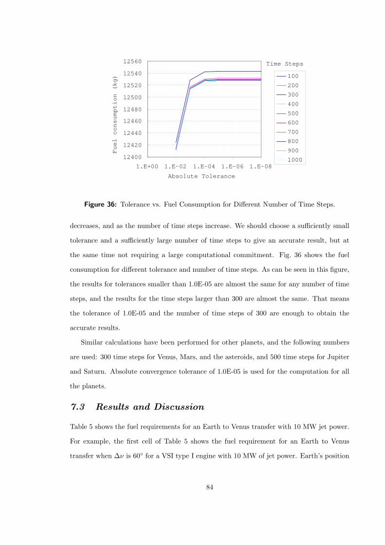
Time Steps
12400
12420
12440
12460
12480
12500
12520
12540
12560
1.E-08 1.E-06 1.E-04 1.E-02 1.E+00
Absolute Tolerance
Fuel consumption (kg) 100
200
300
400
500
600
700
800
900
1000
Figure 36: Tolerance vs. Fuel Consumption for Different Number of Time Steps.
decreases, and as the number of time steps increase. We should choose a sufficiently small
tolerance and a sufficiently large number of time steps to give an accurate result, but at
the same time not requiring a large computational commitment. Fig. 36 shows the fuel
consumption for different tolerance and number of time steps. As can be seen in this figure,
the results for tolerances smaller than 1.0E-05 are almost the same for any number of time
steps, and the results for the time steps larger than 300 are almost the same. That means
the tolerance of 1.0E-05 and the number of time steps of 300 are enough to obtain the
accurate results.
Similar calculations have been performed for other planets, and the following numbers
are used: 300 time steps for Venus, Mars, and the asteroids, and 500 time steps for Jupiter
and Saturn. Absolute convergence tolerance of 1.0E-05 is used for the computation for all
the planets.
7.3 Results and Discussion
Table 5 shows the fuel requirements for an Earth to Venus transfer with 10 MW jet power.
For example, the first cell of Table 5 shows the fuel requirement for an Earth to Venus
transfer when ∆ν is 60 for a VSI type I engine with 10 MW of jet power. Earth’s position
84
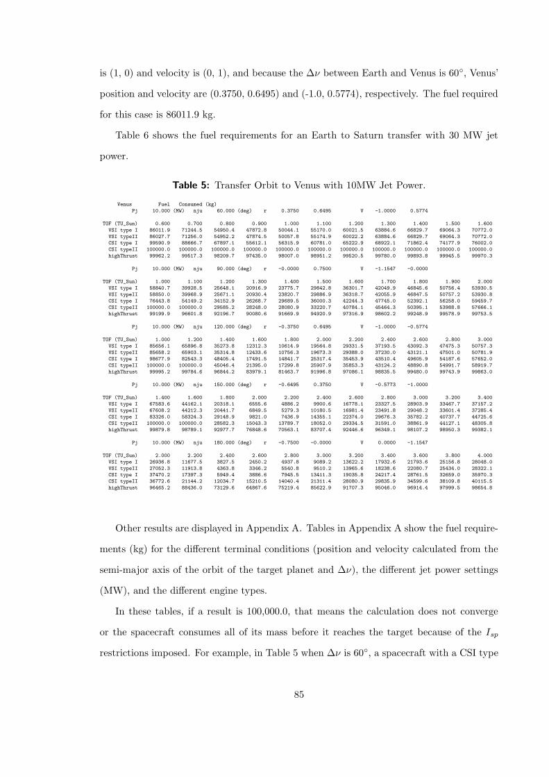
is (1, 0) and velocity is (0, 1), and because the ∆ν between Earth and Venus is 60, Venus’
position and velocity are (0.3750, 0.6495) and (-1.0, 0.5774), respectively. The fuel required
for this case is 86011.9 kg.
Table 6 shows the fuel requirements for an Earth to Saturn transfer with 30 MW jet
power.
Table 5: Transfer Orbit to Venus with 10MW Jet Power.
Venus Fuel Consumed (kg)
Pj 10.000 (MW) nju 60.000 (deg) r 0.3750 0.6495 V -1.0000 0.5774
TOF (TU_Sun) 0.600 0.700 0.800 0.900 1.000 1.100 1.200 1.300 1.400 1.500 1.600
VSI type I 86011.9 71244.5 54950.4 47872.8 50044.1 55170.0 60021.5 63884.6 66829.7 69064.3 70772.0
VSI typeII 86027.7 71256.0 54952.2 47874.5 50057.8 55174.9 60022.2 63884.6 66829.7 69064.3 70772.0
CSI type I 99590.9 88666.7 67897.1 55612.1 56315.9 60781.0 65222.9 68922.1 71862.4 74177.9 76002.0
CSI typeII 100000.0 100000.0 100000.0 100000.0 100000.0 100000.0 100000.0 100000.0 100000.0 100000.0 100000.0
highThrust 99962.2 99517.3 98209.7 97435.0 98007.0 98951.2 99520.5 99780.0 99893.8 99945.5 99970.3
Pj 10.000 (MW) nju 90.000 (deg) r -0.0000 0.7500 V -1.1547 -0.0000
TOF (TU_Sun) 1.000 1.100 1.200 1.300 1.400 1.500 1.600 1.700 1.800 1.900 2.000
VSI type I 58840.7 39928.5 25648.1 20916.9 23775.7 29842.8 36301.7 42049.9 46845.6 50756.4 53930.5
VSI typeII 58850.0 39968.9 25671.1 20930.4 23820.7 29886.9 36318.7 42055.9 46847.5 50757.2 53930.8
CSI type I 76443.8 54149.2 34152.9 26268.7 29689.5 36000.3 42244.3 47745.0 52392.1 56258.0 59459.7
CSI typeII 100000.0 100000.0 29585.2 28248.0 28080.9 33220.7 40784.1 45464.3 50395.1 53988.8 57666.1
highThrust 99199.9 96601.8 92196.7 90080.6 91669.9 94920.9 97316.9 98602.2 99248.9 99578.9 99753.5
Pj 10.000 (MW) nju 120.000 (deg) r -0.3750 0.6495 V -1.0000 -0.5774
TOF (TU_Sun) 1.000 1.200 1.400 1.600 1.800 2.000 2.200 2.400 2.600 2.800 3.000
VSI type I 85656.1 65896.8 35273.8 12312.3 10614.9 19564.8 29331.5 37193.5 43092.3 47475.3 50757.3
VSI typeII 85658.2 65903.1 35314.8 12433.6 10756.3 19673.3 29388.0 37230.0 43121.1 47501.0 50781.9
CSI type I 98677.9 82543.3 48405.4 17491.5 14841.7 25317.4 35453.9 43510.4 49605.9 54187.6 57652.0
CSI typeII 100000.0 100000.0 45046.4 21395.0 17299.8 25907.9 35853.3 43124.2 48890.8 54991.7 58919.7
highThrust 99995.2 99784.6 96844.2 83979.1 81463.7 91996.8 97086.1 98835.5 99480.0 99743.9 99863.0
Pj 10.000 (MW) nju 150.000 (deg) r -0.6495 0.3750 V -0.5773 -1.0000
TOF (TU_Sun) 1.400 1.600 1.800 2.000 2.200 2.400 2.600 2.800 3.000 3.200 3.400
VSI type I 67583.6 44162.1 20318.1 6555.6 4886.2 9900.6 16778.1 23327.5 28903.9 33467.7 37157.2
VSI typeII 67608.2 44212.3 20441.7 6849.5 5279.3 10180.5 16981.4 23491.8 29048.2 33601.4 37285.4
CSI type I 83326.0 58324.3 29148.9 9821.0 7436.9 14355.1 22374.0 29676.3 35782.2 40737.7 44725.6
CSI typeII 100000.0 100000.0 28582.3 15043.3 13789.7 18052.0 29334.5 31591.0 38861.9 44127.1 48305.8
highThrust 99879.8 98789.1 92977.7 76848.6 70563.1 83707.4 92446.6 96349.1 98107.2 98950.3 99382.1
Pj 10.000 (MW) nju 180.000 (deg) r -0.7500 -0.0000 V 0.0000 -1.1547
TOF (TU_Sun) 2.000 2.200 2.400 2.600 2.800 3.000 3.200 3.400 3.600 3.800 4.000
VSI type I 26936.8 11677.5 3827.5 2450.2 4937.8 9089.2 13622.2 17932.6 21793.6 25156.8 28048.0
VSI typeII 27052.3 11913.8 4363.8 3346.2 5540.8 9510.2 13965.6 18238.6 22080.7 25434.0 28322.1
CSI type I 37470.2 17397.3 5949.4 3886.6 7945.5 13411.3 19035.8 24217.4 28761.5 32659.0 35970.3
CSI typeII 36772.6 21144.2 12034.7 15210.5 14040.4 21311.4 28080.9 29835.9 34599.6 38109.8 40115.5
highThrust 96465.2 88436.0 73129.6 64867.6 75219.4 85622.9 91707.3 95046.0 96914.4 97999.5 98654.8
Other results are displayed in Appendix A. Tables in Appendix A show the fuel require-
ments (kg) for the different terminal conditions (position and velocity calculated from the
semi-major axis of the orbit of the target planet and ∆ν), the different jet power settings
(MW), and the different engine types.
In these tables, if a result is 100,000.0, that means the calculation does not converge
or the spacecraft consumes all of its mass before it reaches the target because of the Isp
restrictions imposed. For example, in Table 5 when ∆ν is 60, a spacecraft with a CSI type
85
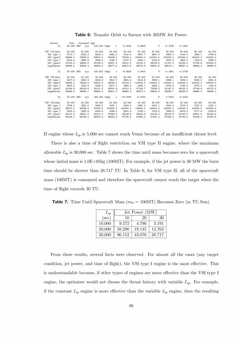
Table 6: Transfer Orbit to Saturn with 30MW Jet Power.
Saturn Fuel Consumed (kg)
Pj 30.000 (MW) nju 120.000 (deg) r -5.0000 8.6603 V -0.2739 -0.1581
TOF (TU_Sun) 20.000 22.000 24.000 26.000 28.000 30.000 32.000 34.000 36.000 38.000 40.000
VSI type I 6772.1 6242.3 5816.0 5455.4 5140.0 4857.7 4601.3 4365.9 4148.5 3946.7 3758.9
VSI typeII 69645.0 76609.5 83574.0 90538.5 97503.0 100000.0 100000.0 100000.0 100000.0 100000.0 100000.0
CSI type I 6516.6 5860.9 4089.3 3195.7 6127.5 2493.1 2419.5 3427.4 3845.5 1918.8 2588.0
CSI typeII 50144.4 49643.0 48138.6 45631.4 49141.5 45130.0 48138.6 51147.3 54156.0 57164.6 100000.0
highThrust 99698.5 99640.2 99600.0 99577.6 99570.8 99576.6 99591.8 99613.1 99637.9 99664.0 99689.9
Pj 30.000 (MW) nju 150.000 (deg) r -8.6603 5.0000 V -0.1581 -0.2739
TOF (TU_Sun) 20.000 22.000 24.000 26.000 28.000 30.000 32.000 34.000 36.000 38.000 40.000
VSI type I 4617.4 4255.5 4002.6 3810.7 3654.4 3519.8 3399.1 3288.1 3184.1 3085.6 2991.8
VSI typeII 69645.0 76609.5 83574.0 90538.5 97503.0 100000.0 100000.0 100000.0 100000.0 100000.0 100000.0
CSI type I 9803.5 5256.5 4229.3 8277.0 3854.2 2294.1 2839.1 9729.8 2769.2 3574.4 1764.6
CSI typeII 50144.4 66190.6 42121.3 45631.4 42121.3 57164.7 72208.0 51147.3 45130.0 57164.6 60173.3
highThrust 99369.4 99086.7 98824.4 98611.2 98460.4 98373.1 98342.9 98358.7 98408.6 98480.9 98566.1
Pj 30.000 (MW) nju 180.000 (deg) r -10.0000 -0.0000 V 0.0000 -0.3162
TOF (TU_Sun) 24.000 26.000 28.000 30.000 32.000 34.000 36.000 38.000 40.000 42.000 44.000
VSI type I 2795.0 2652.5 2556.5 2487.1 2433.0 2387.5 2347.1 2309.4 2273.3 2237.9 2203.1
VSI typeII 83574.0 90538.5 97503.0 100000.0 100000.0 100000.0 100000.0 100000.0 100000.0 100000.0 100000.0
CSI type I 5923.3 4295.8 6359.6 4098.5 8041.8 5758.1 7503.3 2269.8 8679.2 2777.9 5029.6
CSI typeII 42121.3 45631.4 42121.3 67695.0 48138.6 42622.8 54156.0 38109.8 50144.4 52651.6 66190.6
highThrust 99108.2 98745.0 98372.4 98023.9 97725.5 97493.0 97331.2 97236.4 97199.5 97209.0 97253.4
II engine whose Isp is 5,000 sec cannot reach Venus because of an insufficient thrust level.
There is also a time of flight restriction on VSI type II engine, where the maximum
allowable Isp is 30,000 sec. Table 7 shows the time until mass becomes zero for a spacecraft
whose initial mass is 1.0E+05kg (100MT). For example, if the jet power is 30 MW the burn
time should be shorter than 28.717 TU. In Table 6, for VSI type II, all of the spacecraft
mass (100MT) is consumed and therefore the spacecraft cannot reach the target when the
time of flight exceeds 30 TU.
Table 7: Time Until Spacecraft Mass (m0 = 100MT) Becomes Zero (in TU Sun).
Isp Jet Power (MW)(sec) 10 20 30
10,000 9.572 4.786 3.191
20,000 38.290 19.145 12.763
30,000 96.152 43.076 28.717
From these results, several facts were observed. For almost all the cases (any target
condition, jet power, and time of flight), the VSI type I engine is the most effective. This
is understandable because, if other types of engines are more effective than the VSI type I
engine, the optimizer would not choose the thrust history with variable Isp. For example,
if the constant Isp engine is more effective than the variable Isp engine, then the resulting
86
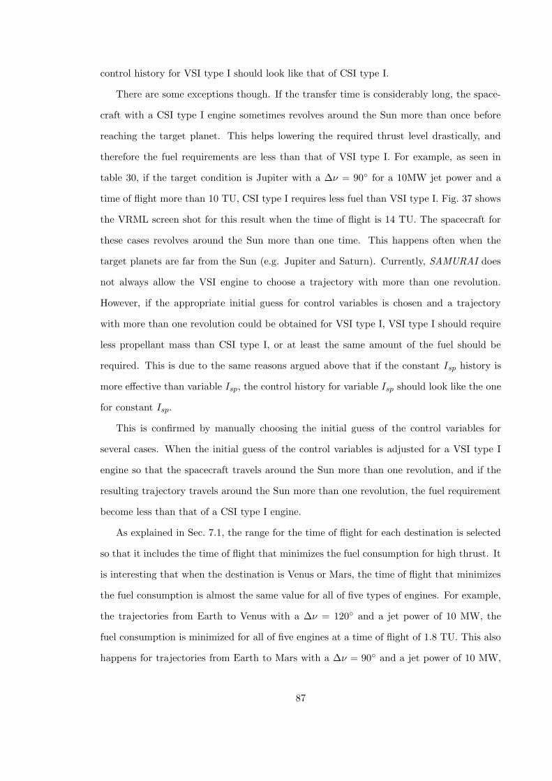
control history for VSI type I should look like that of CSI type I.
There are some exceptions though. If the transfer time is considerably long, the space-
craft with a CSI type I engine sometimes revolves around the Sun more than once before
reaching the target planet. This helps lowering the required thrust level drastically, and
therefore the fuel requirements are less than that of VSI type I. For example, as seen in
table 30, if the target condition is Jupiter with a ∆ν = 90 for a 10MW jet power and a
time of flight more than 10 TU, CSI type I requires less fuel than VSI type I. Fig. 37 shows
the VRML screen shot for this result when the time of flight is 14 TU. The spacecraft for
these cases revolves around the Sun more than one time. This happens often when the
target planets are far from the Sun (e.g. Jupiter and Saturn). Currently, SAMURAI does
not always allow the VSI engine to choose a trajectory with more than one revolution.
However, if the appropriate initial guess for control variables is chosen and a trajectory
with more than one revolution could be obtained for VSI type I, VSI type I should require
less propellant mass than CSI type I, or at least the same amount of the fuel should be
required. This is due to the same reasons argued above that if the constant Isp history is
more effective than variable Isp, the control history for variable Isp should look like the one
for constant Isp.
This is confirmed by manually choosing the initial guess of the control variables for
several cases. When the initial guess of the control variables is adjusted for a VSI type I
engine so that the spacecraft travels around the Sun more than one revolution, and if the
resulting trajectory travels around the Sun more than one revolution, the fuel requirement
become less than that of a CSI type I engine.
As explained in Sec. 7.1, the range for the time of flight for each destination is selected
so that it includes the time of flight that minimizes the fuel consumption for high thrust. It
is interesting that when the destination is Venus or Mars, the time of flight that minimizes
the fuel consumption is almost the same value for all of five types of engines. For example,
the trajectories from Earth to Venus with a ∆ν = 120 and a jet power of 10 MW, the
fuel consumption is minimized for all of five engines at a time of flight of 1.8 TU. This also
happens for trajectories from Earth to Mars with a ∆ν = 90 and a jet power of 10 MW,
87
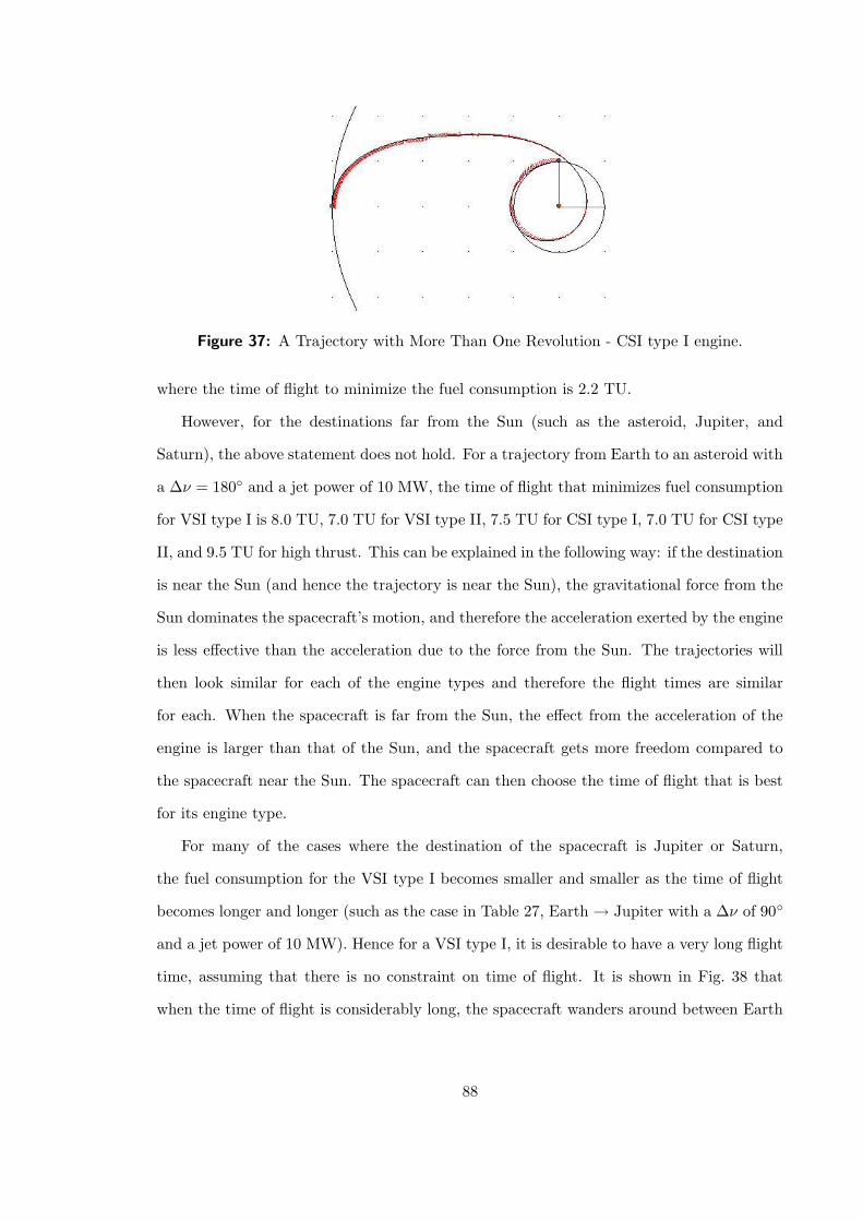
Figure 37: A Trajectory with More Than One Revolution - CSI type I engine.
where the time of flight to minimize the fuel consumption is 2.2 TU.
However, for the destinations far from the Sun (such as the asteroid, Jupiter, and
Saturn), the above statement does not hold. For a trajectory from Earth to an asteroid with
a ∆ν = 180 and a jet power of 10 MW, the time of flight that minimizes fuel consumption
for VSI type I is 8.0 TU, 7.0 TU for VSI type II, 7.5 TU for CSI type I, 7.0 TU for CSI type
II, and 9.5 TU for high thrust. This can be explained in the following way: if the destination
is near the Sun (and hence the trajectory is near the Sun), the gravitational force from the
Sun dominates the spacecraft’s motion, and therefore the acceleration exerted by the engine
is less effective than the acceleration due to the force from the Sun. The trajectories will
then look similar for each of the engine types and therefore the flight times are similar
for each. When the spacecraft is far from the Sun, the effect from the acceleration of the
engine is larger than that of the Sun, and the spacecraft gets more freedom compared to
the spacecraft near the Sun. The spacecraft can then choose the time of flight that is best
for its engine type.
For many of the cases where the destination of the spacecraft is Jupiter or Saturn,
the fuel consumption for the VSI type I becomes smaller and smaller as the time of flight
becomes longer and longer (such as the case in Table 27, Earth → Jupiter with a ∆ν of 90
and a jet power of 10 MW). Hence for a VSI type I, it is desirable to have a very long flight
time, assuming that there is no constraint on time of flight. It is shown in Fig. 38 that
when the time of flight is considerably long, the spacecraft wanders around between Earth
88
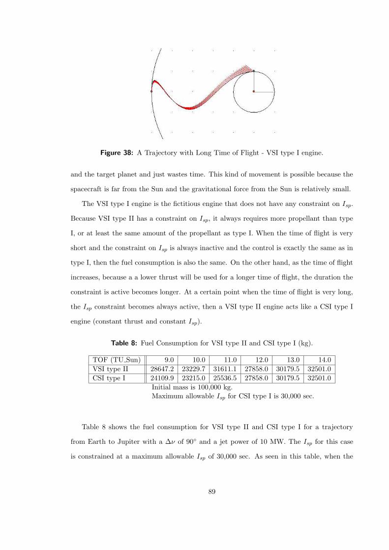
Figure 38: A Trajectory with Long Time of Flight - VSI type I engine.
and the target planet and just wastes time. This kind of movement is possible because the
spacecraft is far from the Sun and the gravitational force from the Sun is relatively small.
The VSI type I engine is the fictitious engine that does not have any constraint on Isp.
Because VSI type II has a constraint on Isp, it always requires more propellant than type
I, or at least the same amount of the propellant as type I. When the time of flight is very
short and the constraint on Isp is always inactive and the control is exactly the same as in
type I, then the fuel consumption is also the same. On the other hand, as the time of flight
increases, because a a lower thrust will be used for a longer time of flight, the duration the
constraint is active becomes longer. At a certain point when the time of flight is very long,
the Isp constraint becomes always active, then a VSI type II engine acts like a CSI type I
engine (constant thrust and constant Isp).
Table 8: Fuel Consumption for VSI type II and CSI type I (kg).
TOF (TU Sun) 9.0 10.0 11.0 12.0 13.0 14.0
VSI type II 28647.2 23229.7 31611.1 27858.0 30179.5 32501.0
CSI type I 24109.9 23215.0 25536.5 27858.0 30179.5 32501.0
Initial mass is 100,000 kg.Maximum allowable Isp for CSI type I is 30,000 sec.
Table 8 shows the fuel consumption for VSI type II and CSI type I for a trajectory
from Earth to Jupiter with a ∆ν of 90 and a jet power of 10 MW. The Isp for this case
is constrained at a maximum allowable Isp of 30,000 sec. As seen in this table, when the
89
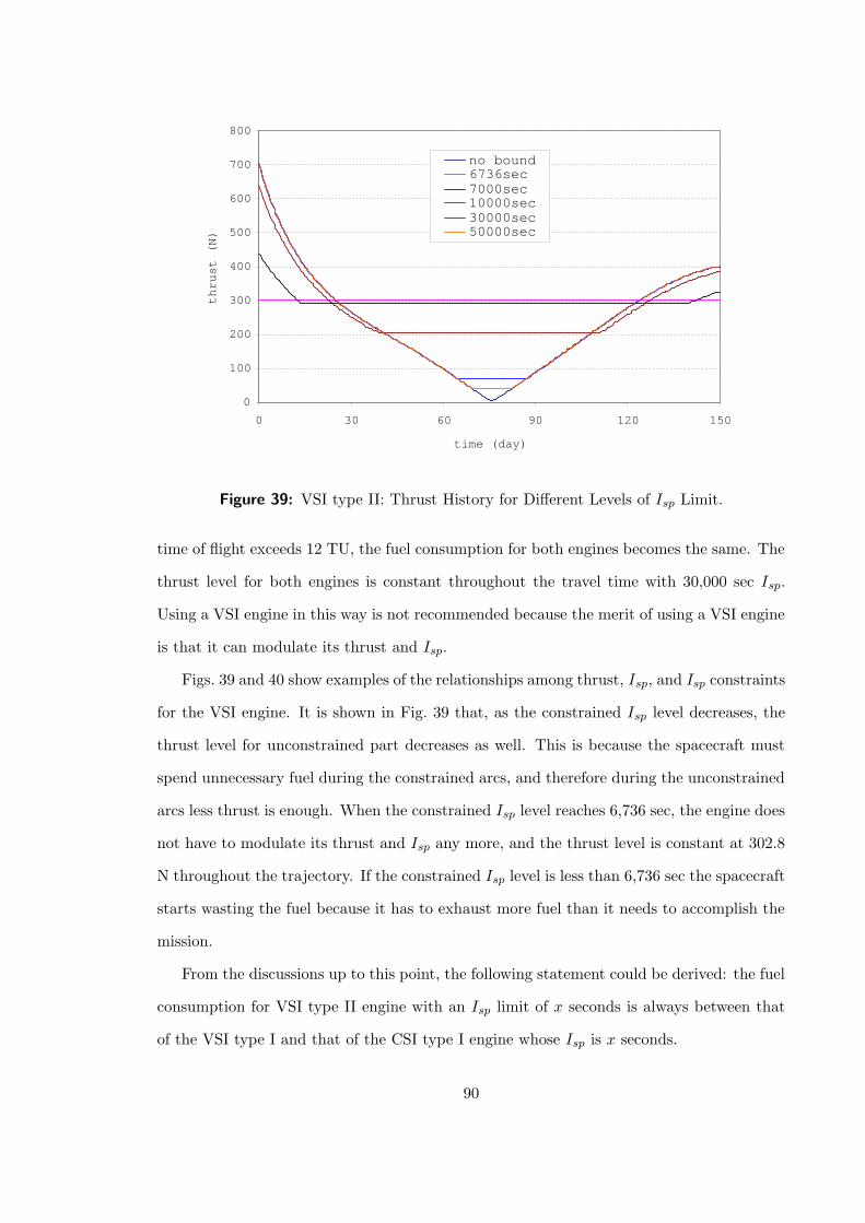
0
100
200
300
400
500
600
700
800
0 30 60 90 120 150
time (day)
thrust (N)
no bound 6736sec 7000sec 10000sec 30000sec 50000sec
Figure 39: VSI type II: Thrust History for Different Levels of Isp Limit.
time of flight exceeds 12 TU, the fuel consumption for both engines becomes the same. The
thrust level for both engines is constant throughout the travel time with 30,000 sec Isp.
Using a VSI engine in this way is not recommended because the merit of using a VSI engine
is that it can modulate its thrust and Isp.
Figs. 39 and 40 show examples of the relationships among thrust, Isp, and Isp constraints
for the VSI engine. It is shown in Fig. 39 that, as the constrained Isp level decreases, the
thrust level for unconstrained part decreases as well. This is because the spacecraft must
spend unnecessary fuel during the constrained arcs, and therefore during the unconstrained
arcs less thrust is enough. When the constrained Isp level reaches 6,736 sec, the engine does
not have to modulate its thrust and Isp any more, and the thrust level is constant at 302.8
N throughout the trajectory. If the constrained Isp level is less than 6,736 sec the spacecraft
starts wasting the fuel because it has to exhaust more fuel than it needs to accomplish the
mission.
From the discussions up to this point, the following statement could be derived: the fuel
consumption for VSI type II engine with an Isp limit of x seconds is always between that
of the VSI type I and that of the CSI type I engine whose Isp is x seconds.
90
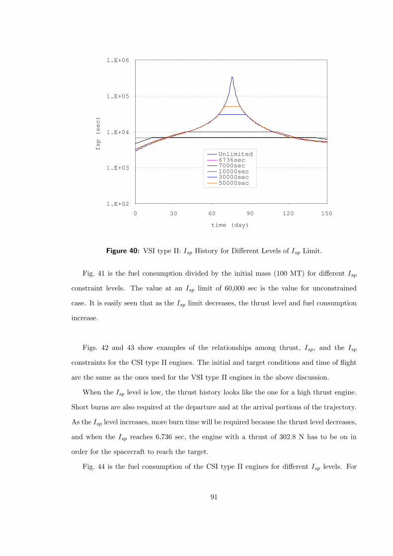
1.E+02
1.E+03
1.E+04
1.E+05
1.E+06
0 30 60 90 120 150
time (day)
Isp (sec)
Unlimited 6736sec 7000sec 10000sec 30000sec 50000sec
Figure 40: VSI type II: Isp History for Different Levels of Isp Limit.
Fig. 41 is the fuel consumption divided by the initial mass (100 MT) for different Isp
constraint levels. The value at an Isp limit of 60,000 sec is the value for unconstrained
case. It is easily seen that as the Isp limit decreases, the thrust level and fuel consumption
increase.
Figs. 42 and 43 show examples of the relationships among thrust, Isp, and the Isp
constraints for the CSI type II engines. The initial and target conditions and time of flight
are the same as the ones used for the VSI type II engines in the above discussion.
When the Isp level is low, the thrust history looks like the one for a high thrust engine.
Short burns are also required at the departure and at the arrival portions of the trajectory.
As the Isp level increases, more burn time will be required because the thrust level decreases,
and when the Isp reaches 6,736 sec, the engine with a thrust of 302.8 N has to be on in
order for the spacecraft to reach the target.
Fig. 44 is the fuel consumption of the CSI type II engines for different Isp levels. For
91
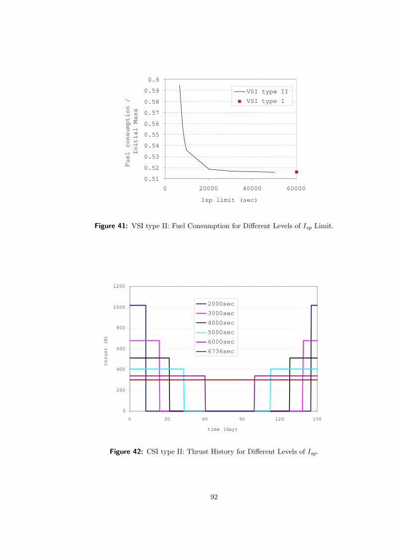
0.51
0.52
0.53
0.54
0.55
0.56
0.57
0.58
0.59
0.6
0 20000 40000 60000
Isp limit (sec)
Fuel consumption /
Initial Mass
VSI type II
VSI type I
Figure 41: VSI type II: Fuel Consumption for Different Levels of Isp Limit.
0
200
400
600
800
1000
1200
0 30 60 90 120 150
time (day)
thrust (N)
2000sec
3000sec
4000sec
5000sec
6000sec
6736sec
Figure 42: CSI type II: Thrust History for Different Levels of Isp.
92
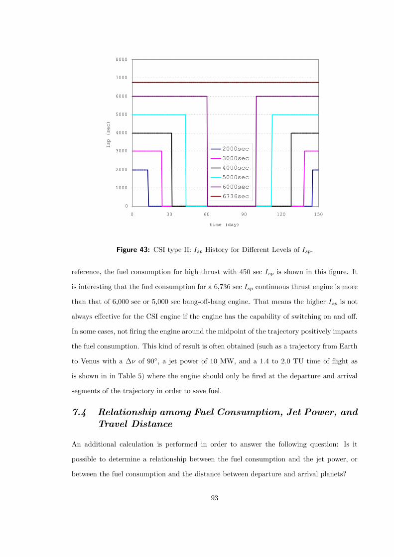
0
1000
2000
3000
4000
5000
6000
7000
8000
0 30 60 90 120 150
time (day)
Isp (sec)
2000sec
3000sec
4000sec
5000sec
6000sec
6736sec
Figure 43: CSI type II: Isp History for Different Levels of Isp.
reference, the fuel consumption for high thrust with 450 sec Isp is shown in this figure. It
is interesting that the fuel consumption for a 6,736 sec Isp continuous thrust engine is more
than that of 6,000 sec or 5,000 sec bang-off-bang engine. That means the higher Isp is not
always effective for the CSI engine if the engine has the capability of switching on and off.
In some cases, not firing the engine around the midpoint of the trajectory positively impacts
the fuel consumption. This kind of result is often obtained (such as a trajectory from Earth
to Venus with a ∆ν of 90, a jet power of 10 MW, and a 1.4 to 2.0 TU time of flight as
is shown in in Table 5) where the engine should only be fired at the departure and arrival
segments of the trajectory in order to save fuel.
7.4 Relationship among Fuel Consumption, Jet Power, and
Travel Distance
An additional calculation is performed in order to answer the following question: Is it
possible to determine a relationship between the fuel consumption and the jet power, or
between the fuel consumption and the distance between departure and arrival planets?
93
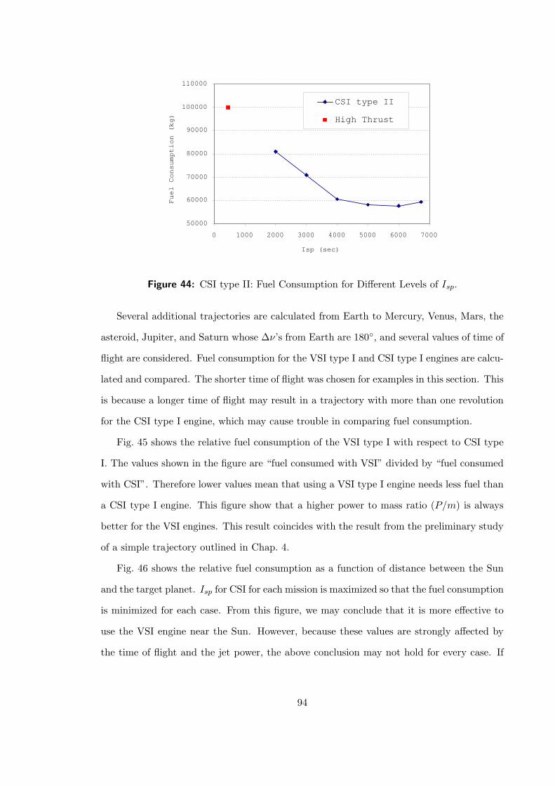
50000
60000
70000
80000
90000
100000
110000
0 1000 2000 3000 4000 5000 6000 7000
Isp (sec)
Fuel Consumption (kg)
CSI type II
High Thrust
Figure 44: CSI type II: Fuel Consumption for Different Levels of Isp.
Several additional trajectories are calculated from Earth to Mercury, Venus, Mars, the
asteroid, Jupiter, and Saturn whose ∆ν’s from Earth are 180, and several values of time of
flight are considered. Fuel consumption for the VSI type I and CSI type I engines are calcu-
lated and compared. The shorter time of flight was chosen for examples in this section. This
is because a longer time of flight may result in a trajectory with more than one revolution
for the CSI type I engine, which may cause trouble in comparing fuel consumption.
Fig. 45 shows the relative fuel consumption of the VSI type I with respect to CSI type
I. The values shown in the figure are “fuel consumed with VSI” divided by “fuel consumed
with CSI”. Therefore lower values mean that using a VSI type I engine needs less fuel than
a CSI type I engine. This figure show that a higher power to mass ratio (P/m) is always
better for the VSI engines. This result coincides with the result from the preliminary study
of a simple trajectory outlined in Chap. 4.
Fig. 46 shows the relative fuel consumption as a function of distance between the Sun
and the target planet. Isp for CSI for each mission is maximized so that the fuel consumption
is minimized for each case. From this figure, we may conclude that it is more effective to
use the VSI engine near the Sun. However, because these values are strongly affected by
the time of flight and the jet power, the above conclusion may not hold for every case. If
94
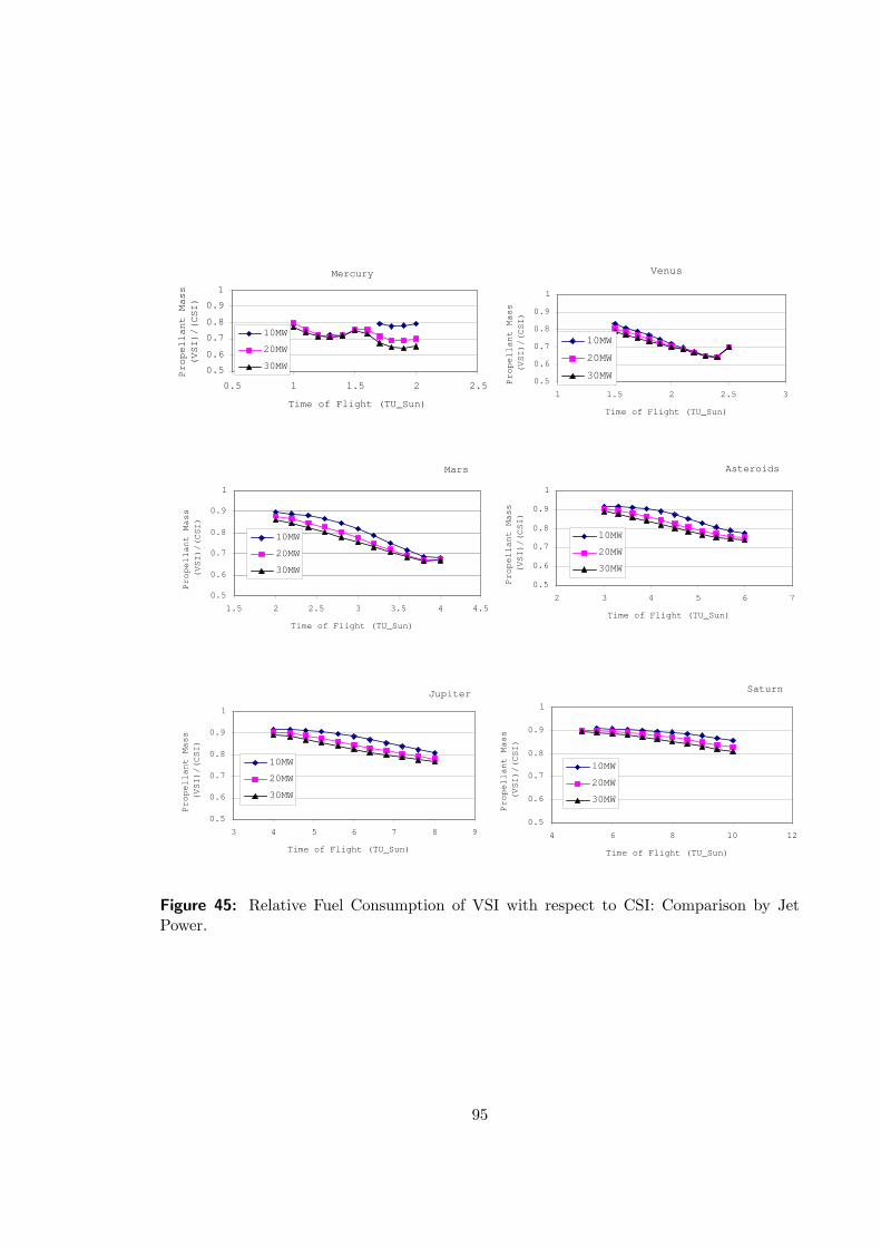
Mars
0.5
0.6
0.7
0.8
0.9
1
1.5 2 2.5 3 3.5 4 4.5
Time of Flight (TU_Sun)
Propellant Mass
(VSI)/(CSI)
10MW
20MW
30MW
Asteroids
0.5
0.6
0.7
0.8
0.9
1
2 3 4 5 6 7
Time of Flight (TU_Sun)
Propellant Mass
(VSI)/(CSI)
10MW
20MW
30MW
Jupiter
0.5
0.6
0.7
0.8
0.9
1
3 4 5 6 7 8 9
Time of Flight (TU_Sun)
Propellant Mass
(VSI)/(CSI)
10MW
20MW
30MW
Saturn
0.5
0.6
0.7
0.8
0.9
1
4 6 8 10 12
Time of Flight (TU_Sun)
Propellant Mass
(VSI)/(CSI)
10MW
20MW
30MW
Venus
0.5
0.6
0.7
0.8
0.9
1
1 1.5 2 2.5 3
Time of Flight (TU_Sun)
Propellant Mass
(VSI)/(CSI)
10MW
20MW
30MW
Mercury
0.5
0.6
0.7
0.8
0.9
1
0.5 1 1.5 2 2.5
Time of Flight (TU_Sun)
Propellant Mass
(VSI)/(CSI)
10MW
20MW
30MW
Figure 45: Relative Fuel Consumption of VSI with respect to CSI: Comparison by JetPower.
95
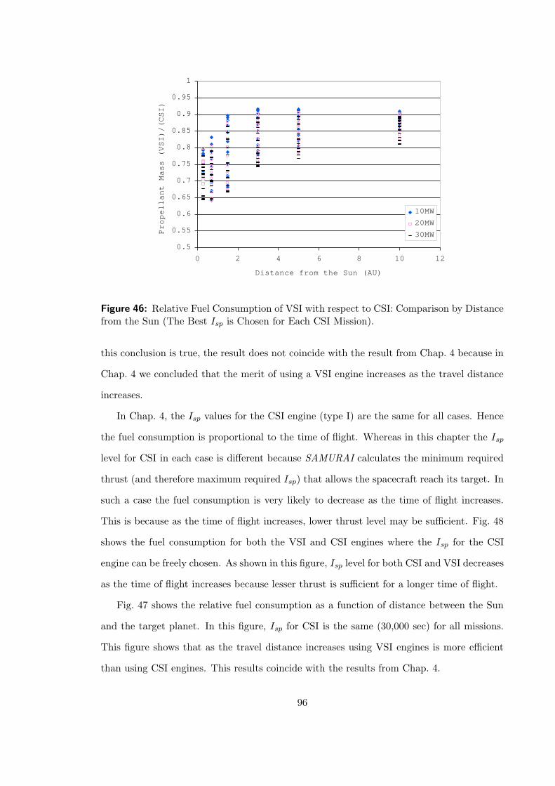
0.5
0.55
0.6
0.65
0.7
0.75
0.8
0.85
0.9
0.95
1
0 2 4 6 8 10 12
Distance from the Sun (AU)
Propellant Mass (VSI)/(CSI)
10MW
20MW
30MW
Figure 46: Relative Fuel Consumption of VSI with respect to CSI: Comparison by Distancefrom the Sun (The Best Isp is Chosen for Each CSI Mission).
this conclusion is true, the result does not coincide with the result from Chap. 4 because in
Chap. 4 we concluded that the merit of using a VSI engine increases as the travel distance
increases.
In Chap. 4, the Isp values for the CSI engine (type I) are the same for all cases. Hence
the fuel consumption is proportional to the time of flight. Whereas in this chapter the Isp
level for CSI in each case is different because SAMURAI calculates the minimum required
thrust (and therefore maximum required Isp) that allows the spacecraft reach its target. In
such a case the fuel consumption is very likely to decrease as the time of flight increases.
This is because as the time of flight increases, lower thrust level may be sufficient. Fig. 48
shows the fuel consumption for both the VSI and CSI engines where the Isp for the CSI
engine can be freely chosen. As shown in this figure, Isp level for both CSI and VSI decreases
as the time of flight increases because lesser thrust is sufficient for a longer time of flight.
Fig. 47 shows the relative fuel consumption as a function of distance between the Sun
and the target planet. In this figure, Isp for CSI is the same (30,000 sec) for all missions.
This figure shows that as the travel distance increases using VSI engines is more efficient
than using CSI engines. This results coincide with the results from Chap. 4.
96
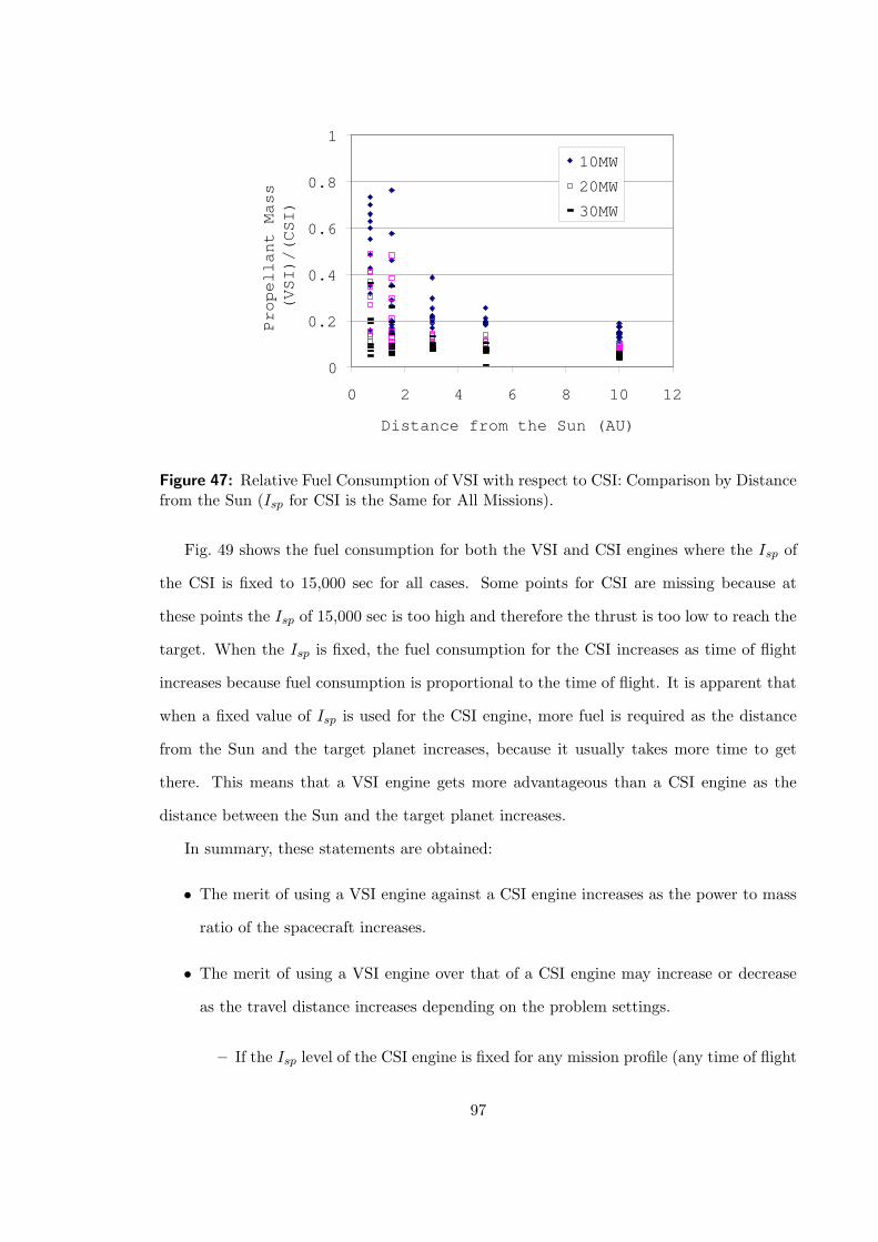
0
0.2
0.4
0.6
0.8
1
0 2 4 6 8 10 12
Distance from the Sun (AU)
Propellant Mass
(VSI)/(CSI)
10MW
20MW
30MW
Figure 47: Relative Fuel Consumption of VSI with respect to CSI: Comparison by Distancefrom the Sun (Isp for CSI is the Same for All Missions).
Fig. 49 shows the fuel consumption for both the VSI and CSI engines where the Isp of
the CSI is fixed to 15,000 sec for all cases. Some points for CSI are missing because at
these points the Isp of 15,000 sec is too high and therefore the thrust is too low to reach the
target. When the Isp is fixed, the fuel consumption for the CSI increases as time of flight
increases because fuel consumption is proportional to the time of flight. It is apparent that
when a fixed value of Isp is used for the CSI engine, more fuel is required as the distance
from the Sun and the target planet increases, because it usually takes more time to get
there. This means that a VSI engine gets more advantageous than a CSI engine as the
distance between the Sun and the target planet increases.
In summary, these statements are obtained:
• The merit of using a VSI engine against a CSI engine increases as the power to mass
ratio of the spacecraft increases.
• The merit of using a VSI engine over that of a CSI engine may increase or decrease
as the travel distance increases depending on the problem settings.
– If the Isp level of the CSI engine is fixed for any mission profile (any time of flight
97
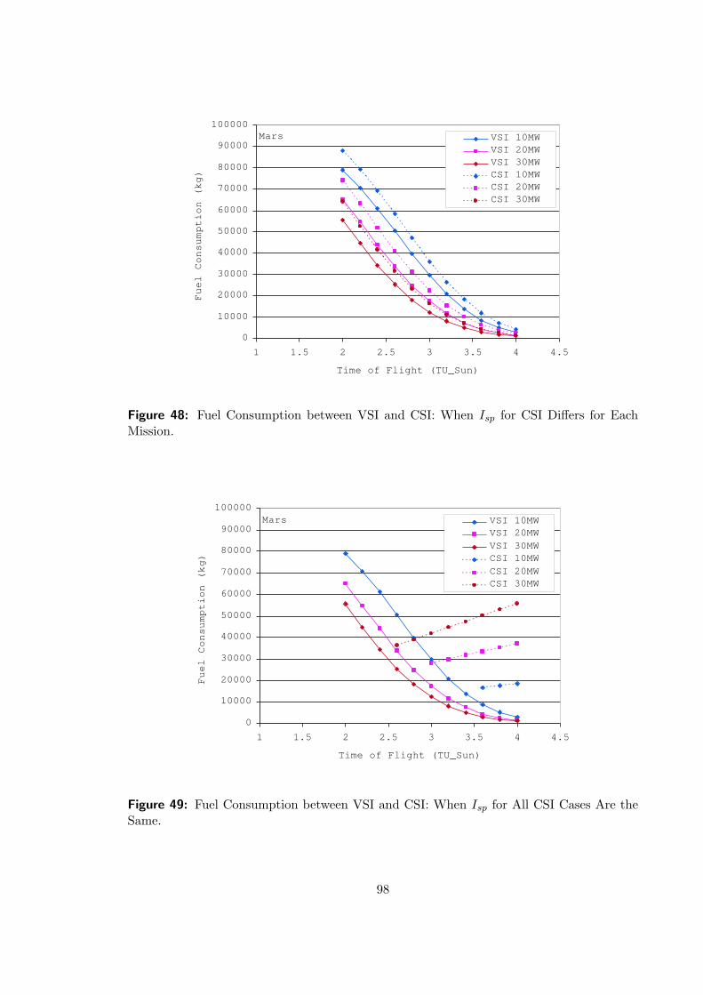
Mars
0
10000
20000
30000
40000
50000
60000
70000
80000
90000
100000
1 1.5 2 2.5 3 3.5 4 4.5
Time of Flight (TU_Sun)
Fuel Consumption (kg)
VSI 10MWVSI 20MWVSI 30MWCSI 10MWCSI 20MWCSI 30MW
Figure 48: Fuel Consumption between VSI and CSI: When Isp for CSI Differs for EachMission.
Mars
0
10000
20000
30000
40000
50000
60000
70000
80000
90000
100000
1 1.5 2 2.5 3 3.5 4 4.5
Time of Flight (TU_Sun)
Fuel Consumption (kg)
VSI 10MWVSI 20MWVSI 30MWCSI 10MWCSI 20MWCSI 30MW
Figure 49: Fuel Consumption between VSI and CSI: When Isp for All CSI Cases Are theSame.
98
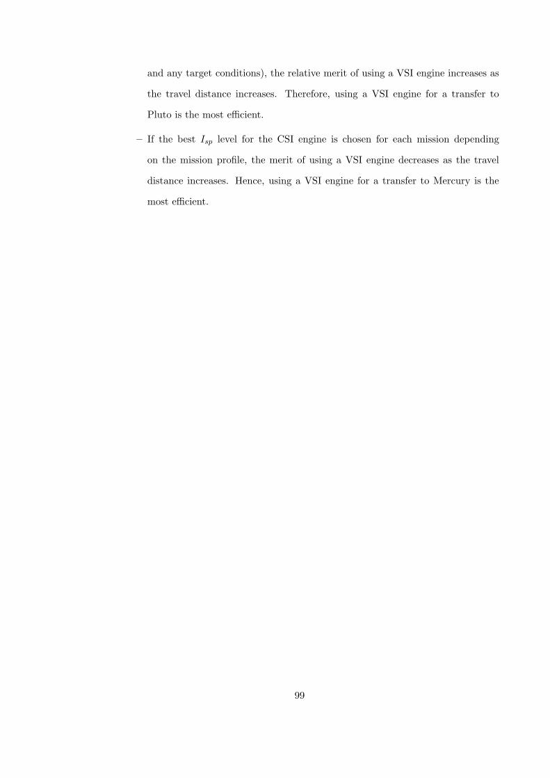
and any target conditions), the relative merit of using a VSI engine increases as
the travel distance increases. Therefore, using a VSI engine for a transfer to
Pluto is the most efficient.
– If the best Isp level for the CSI engine is chosen for each mission depending
on the mission profile, the merit of using a VSI engine decreases as the travel
distance increases. Hence, using a VSI engine for a transfer to Mercury is the
most efficient.
99
CHAPTER VIII
NUMERICAL EXAMPLES: “REAL WORLD” PROBLEMS
In this chapter, the real ephemeris of planets is used to calculate the transfer trajectories
from Earth to various planets. Engines considered in this chapter are VSI type II (con-
strained Isp) with maximum allowable Isp of 30,000 sec, CSI type I (continuous thrust),
CSI type II (bang-off-bang) with 5,000 sec Isp, and high thrust with 450 sec Isp.
Although the result of the VSI type I engine with no constraint on Isp (and therefore
unrealistic) was not compared with the results of other types of engines, it was used to
estimate the departure date and time of flight that minimize fuel consumption for other
types of engines because computationally the VSI type I can be solved faster. As stated in
the last chapter, the value of time of flight that minimizes the fuel consumption is sometimes
the same for each engine type, and therefore the result of the VSI type I is useful. Ten
MW’s of jet power is assumed for all cases.
Before going to the actual calculations, the concept of “synodic period” is introduced.
A synodic period is defined as the time required for any phase angle between two planets
to repeat itself [12]. This parameter is used to determine the launch opportunity. For two
planets whose periods are p and q, the synodic period is expressed as 1/(1/p − 1/q) =
pq/(q − p). If we miss a particular launch opportunity, we must wait until a desirable
phase angle comes around again. For example, the synodic period of Earth and Mars
is 780 days (2.14 years), and Earth and Venus is 584 days (1.6 years). So if we miss a
launch opportunity to Mars, we have to wait until the next opportunity comes 2.14 years
later. Usually transfer trajectory calculation for one synodic period is enough because fuel
requirements show repetitive patterns for each synodic period.
100
8.1 Scientific Mission to Venus
8.1.1 Venus Exploration
If Earth had a twin, it would be Venus. Venus is sometimes called Earth’s “sister planet.”
The two planets are similar in size, mass, composition, and distance from the Sun. But
there are also many differences. Venus has no oceans, and it is covered by thick, rapidly
spinning clouds that trap surface heat. Therefore the surface temperature is over 450 C,
hotter than the surface of the planet Mercury. The high density of the atmosphere results
in a surface pressure 90 times that of Earth. Because Venus reflects so much sunlight, it is
usually the brightest planet in the sky.
Several probes have been sent to Venus so far. Two of them landed on the Venusian
surface. The Magellan probe, launched in 1989, was the last spacecraft sent to Venus. This
is partly because Venus seems less interesting than Mars and other outer planets. However,
the ESA (European Space Agency) is planning to launch a Venus orbiter mission named
“Venus Express (VEX)” in November 2005.
8.1.2 Problem Description
Because the synodic period of Earth and Venus is 584 days, a grid search for launch date
is performed for a 600-day range starting from Jan. 1, 2010. At first a wide range in time
of flight is considered, then this range is narrowed down to an appropriate value, and the
state and control variables for minimum fuel transfer for each engine type were analyzed.
The initial mass of the spacecraft is set to 100 MT.
8.1.3 Results
Fig. 50 shows the normalized fuel requirements for VSI type II with a 30,000 sec Isp con-
straint. A 600-day range of launch dates starting from Jan. 1, 2010, with the time of flight
between 100 and 300 days are calculated. A resulting value of 1.0 means either the program
failed to calculate the results, or the mass becomes zero before reaching Venus. As shown
in this figure, there is a region with very low values. For example, if the spacecraft leaves
Earth on Aug. 1, 2010, and time of flight is 160 days, the fuel requirement is just 3,195 kg.
101
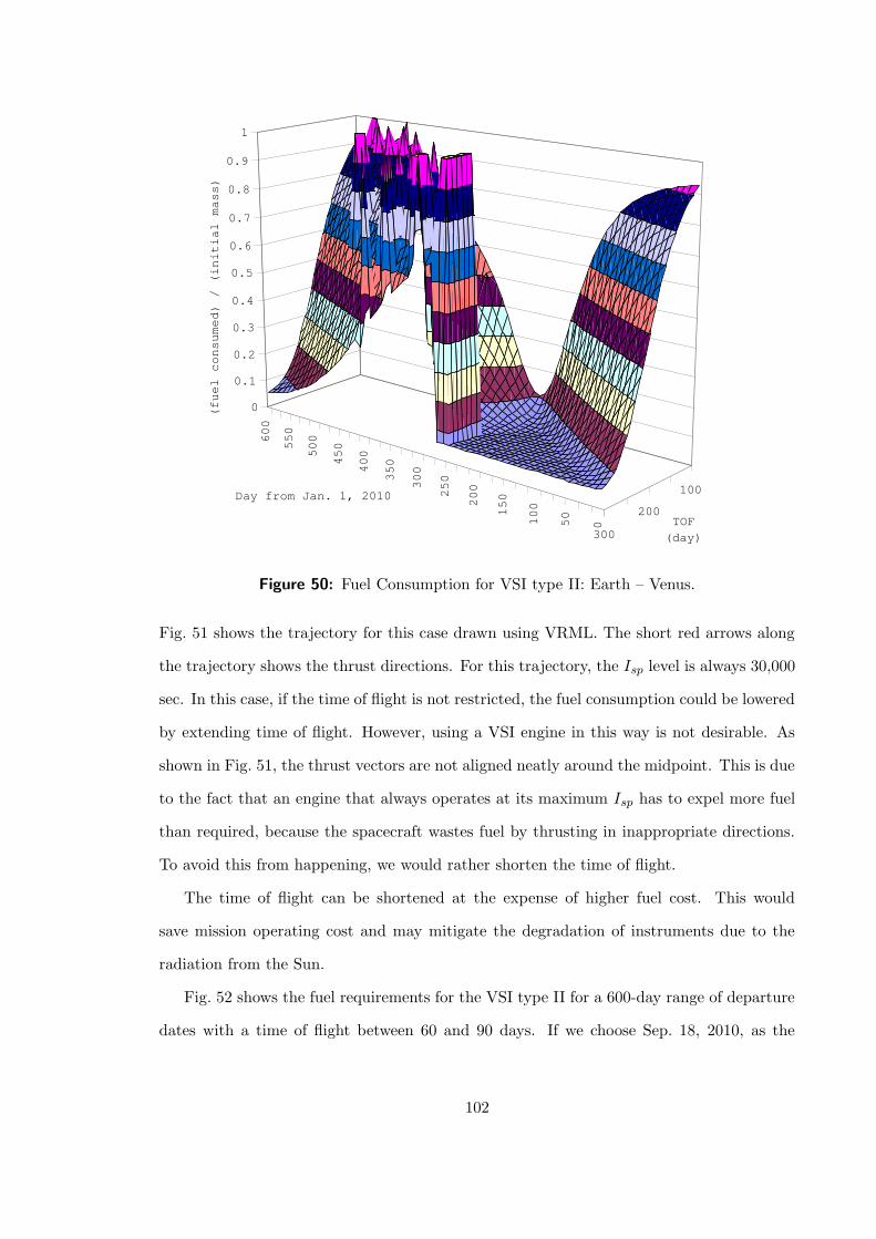
0 50
100
150
200
250
300
350
400
450
500
550
600
100
200
300
0
0.1
0.2
0.3
0.4
0.5
0.6
0.7
0.8
0.9
1
(fuel consumed) / (initial mass)
Day from Jan. 1, 2010
TOF (day)
Figure 50: Fuel Consumption for VSI type II: Earth – Venus.
Fig. 51 shows the trajectory for this case drawn using VRML. The short red arrows along
the trajectory shows the thrust directions. For this trajectory, the Isp level is always 30,000
sec. In this case, if the time of flight is not restricted, the fuel consumption could be lowered
by extending time of flight. However, using a VSI engine in this way is not desirable. As
shown in Fig. 51, the thrust vectors are not aligned neatly around the midpoint. This is due
to the fact that an engine that always operates at its maximum Isp has to expel more fuel
than required, because the spacecraft wastes fuel by thrusting in inappropriate directions.
To avoid this from happening, we would rather shorten the time of flight.
The time of flight can be shortened at the expense of higher fuel cost. This would
save mission operating cost and may mitigate the degradation of instruments due to the
radiation from the Sun.
Fig. 52 shows the fuel requirements for the VSI type II for a 600-day range of departure
dates with a time of flight between 60 and 90 days. If we choose Sep. 18, 2010, as the
102

Figure 51: Trajectory from Earth to Venus with 160-day Time of Flight.
0
0.1
0.2
0.3
0.4
0.5
0.6
0.7
0.8
0.9
1
0 100 200 300 400 500 600
Day from Jan. 1, 2010
(fuel consumed) / (initial mass)
60day
70day
80day
90day
Figure 52: Fuel Consumption for VSI type II: Earth – Venus.
103
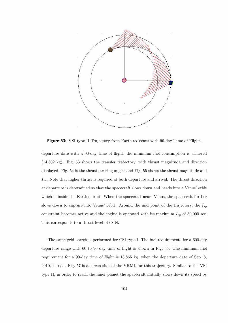
Figure 53: VSI type II Trajectory from Earth to Venus with 90-day Time of Flight.
departure date with a 90-day time of flight, the minimum fuel consumption is achieved
(14,302 kg). Fig. 53 shows the transfer trajectory, with thrust magnitude and direction
displayed. Fig. 54 is the thrust steering angles and Fig. 55 shows the thrust magnitude and
Isp. Note that higher thrust is required at both departure and arrival. The thrust direction
at departure is determined so that the spacecraft slows down and heads into a Venus’ orbit
which is inside the Earth’s orbit. When the spacecraft nears Venus, the spacecraft further
slows down to capture into Venus’ orbit. Around the mid point of the trajectory, the Isp
constraint becomes active and the engine is operated with its maximum Isp of 30,000 sec.
This corresponds to a thrust level of 68 N.
The same grid search is performed for CSI type I. The fuel requirements for a 600-day
departure range with 60 to 90 day time of flight is shown in Fig. 56. The minimum fuel
requirement for a 90-day time of flight is 18,865 kg, when the departure date of Sep. 8,
2010, is used. Fig. 57 is a screen shot of the VRML for this trajectory. Similar to the VSI
type II, in order to reach the inner planet the spacecraft initially slows down its speed by
104
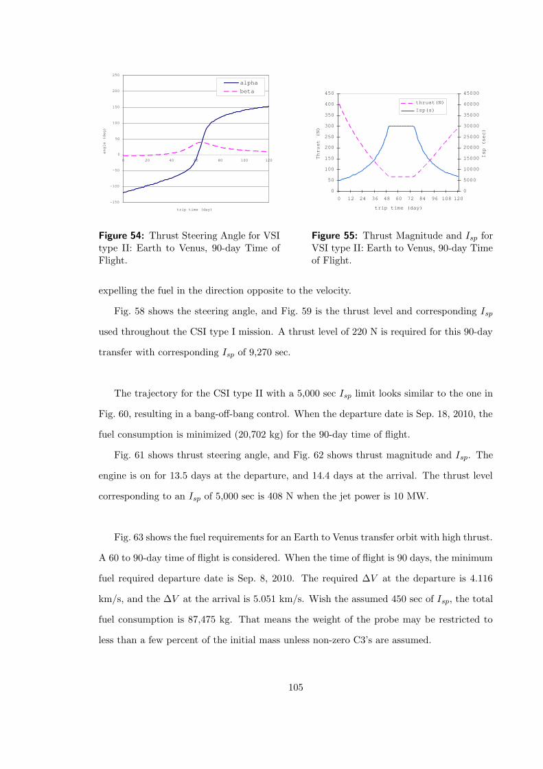
-150
-100
-50
0
50
100
150
200
250
0 20 40 60 80 100 120
trip time (day)
angle (deg)
alpha
beta
Figure 54: Thrust Steering Angle for VSItype II: Earth to Venus, 90-day Time ofFlight.
0
50
100
150
200
250
300
350
400
450
0 12 24 36 48 60 72 84 96 108 120
trip time (day)
Thrust (N)
0
5000
10000
15000
20000
25000
30000
35000
40000
45000
Isp (sec)
thrust(N)
Isp(s)
Figure 55: Thrust Magnitude and Isp forVSI type II: Earth to Venus, 90-day Timeof Flight.
expelling the fuel in the direction opposite to the velocity.
Fig. 58 shows the steering angle, and Fig. 59 is the thrust level and corresponding Isp
used throughout the CSI type I mission. A thrust level of 220 N is required for this 90-day
transfer with corresponding Isp of 9,270 sec.
The trajectory for the CSI type II with a 5,000 sec Isp limit looks similar to the one in
Fig. 60, resulting in a bang-off-bang control. When the departure date is Sep. 18, 2010, the
fuel consumption is minimized (20,702 kg) for the 90-day time of flight.
Fig. 61 shows thrust steering angle, and Fig. 62 shows thrust magnitude and Isp. The
engine is on for 13.5 days at the departure, and 14.4 days at the arrival. The thrust level
corresponding to an Isp of 5,000 sec is 408 N when the jet power is 10 MW.
Fig. 63 shows the fuel requirements for an Earth to Venus transfer orbit with high thrust.
A 60 to 90-day time of flight is considered. When the time of flight is 90 days, the minimum
fuel required departure date is Sep. 8, 2010. The required ∆V at the departure is 4.116
km/s, and the ∆V at the arrival is 5.051 km/s. Wish the assumed 450 sec of Isp, the total
fuel consumption is 87,475 kg. That means the weight of the probe may be restricted to
less than a few percent of the initial mass unless non-zero C3’s are assumed.
105
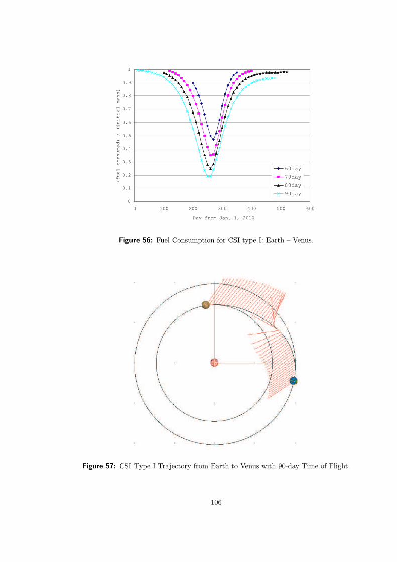
0
0.1
0.2
0.3
0.4
0.5
0.6
0.7
0.8
0.9
1
0 100 200 300 400 500 600
Day from Jan. 1, 2010
(fuel consumed) / (initial mass)
60day
70day
80day
90day
Figure 56: Fuel Consumption for CSI type I: Earth – Venus.
Figure 57: CSI Type I Trajectory from Earth to Venus with 90-day Time of Flight.
106
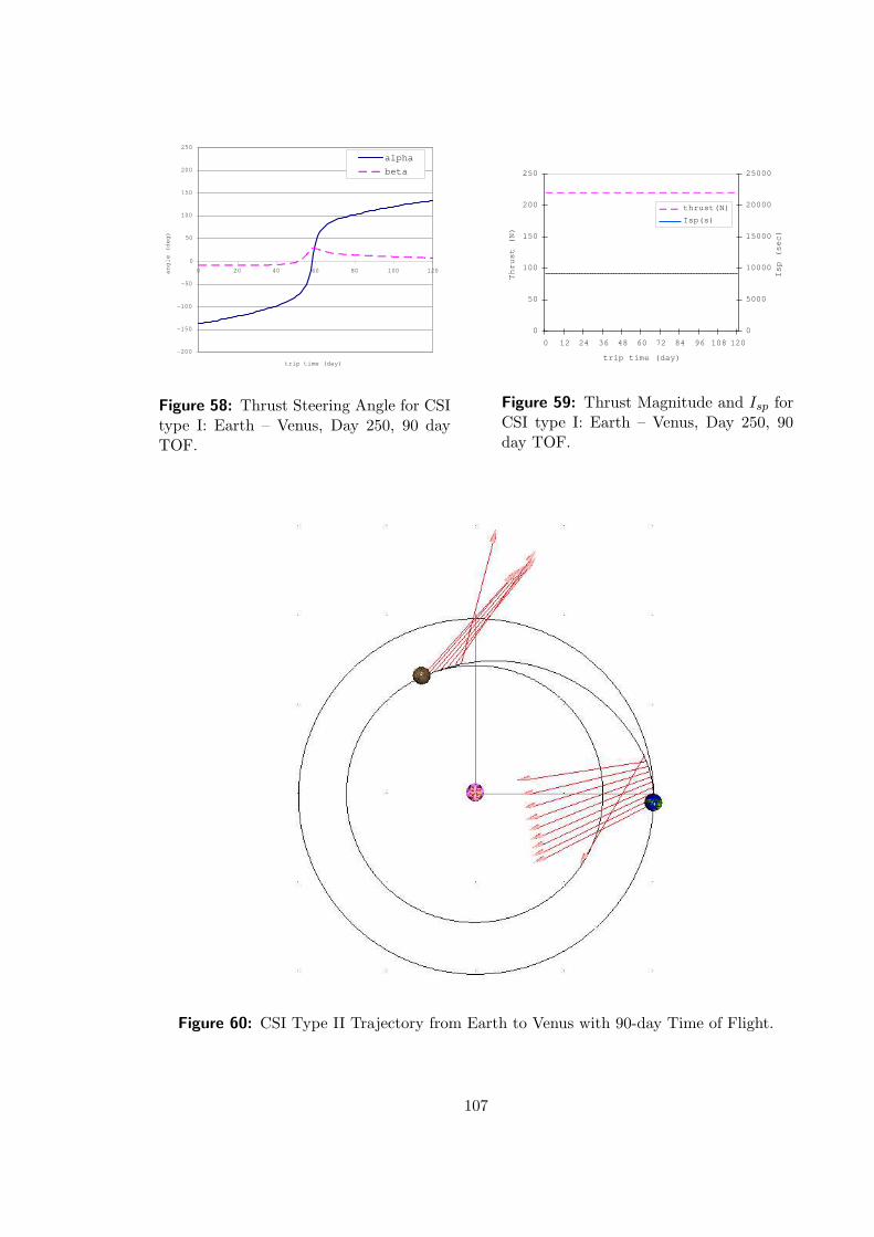
-200
-150
-100
-50
0
50
100
150
200
250
0 20 40 60 80 100 120
trip time (day)
angle (deg)
alpha
beta
Figure 58: Thrust Steering Angle for CSItype I: Earth – Venus, Day 250, 90 dayTOF.
0
50
100
150
200
250
0 12 24 36 48 60 72 84 96 108 120
trip time (day)
Thrust (N)
0
5000
10000
15000
20000
25000
Isp (sec)
thrust(N)
Isp(s)
Figure 59: Thrust Magnitude and Isp forCSI type I: Earth – Venus, Day 250, 90day TOF.
Figure 60: CSI Type II Trajectory from Earth to Venus with 90-day Time of Flight.
107
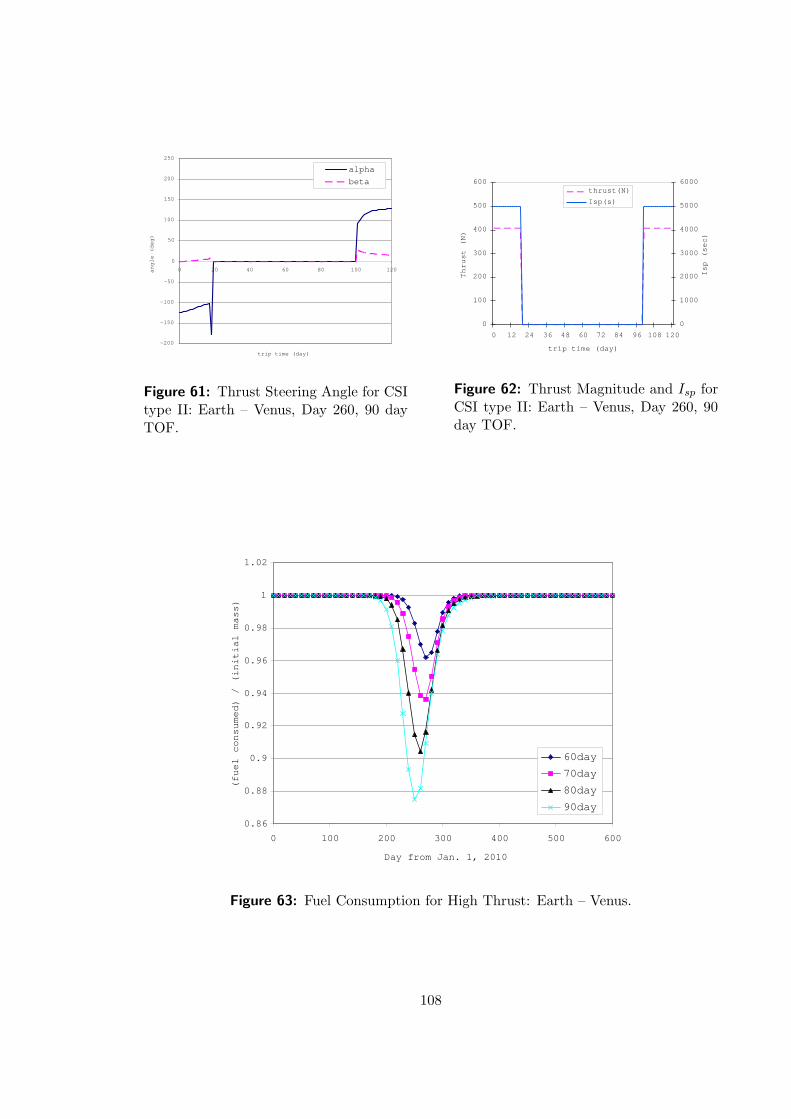
-200
-150
-100
-50
0
50
100
150
200
250
0 20 40 60 80 100 120
trip time (day)
angle (deg)
alpha
beta
Figure 61: Thrust Steering Angle for CSItype II: Earth – Venus, Day 260, 90 dayTOF.
0
100
200
300
400
500
600
0 12 24 36 48 60 72 84 96 108 120
trip time (day)
Thrust (N)
0
1000
2000
3000
4000
5000
6000
Isp (sec)
thrust(N)
Isp(s)
Figure 62: Thrust Magnitude and Isp forCSI type II: Earth – Venus, Day 260, 90day TOF.
0.86
0.88
0.9
0.92
0.94
0.96
0.98
1
1.02
0 100 200 300 400 500 600
Day from Jan. 1, 2010
(fuel consumed) / (initial mass)
60day
70day
80day
90day
Figure 63: Fuel Consumption for High Thrust: Earth – Venus.
108
These results concluded that the VSI type II is most effective engine (least fuel required).
As concluded in the last chapter, the departure date that minimizes the fuel requirements,
is almost the same for all engine types.
8.2 Human Mission to Mars: Round Trip
8.2.1 Mars Exploration
Outside of the Earth-Moon system, Mars is the most hospitable body in the solar system
for humans and is currently the only real candidate for future human exploration and
colonization [1].
In August of 1992, a ”Why Mars” workshop was held in Houston, Texas. Six major
elements behind the motivation for human Mars exploration were introduced by a consultant
team consisting of 16 professionals from across the country.
• Human Evolution – Mars is the next logical step in the expansion of the human race
into the stars.
• Comparative Planetology – by understanding Mars and its evolution as a planet, a
better understanding of Earth will be achieved.
• International Cooperation – an international Mars exploration effort has the potential
to bring about a sense of global unity as never seen before.
• Technological Advancement – the development of new and improved technologies for
the Mars mission will enhance the lives of those on Earth while encouraging high-tech
industry.
• Inspiration – the human Mars exploration mission will test our technological abilities
to their maximum. The ingenuity of the mobilized populace will be tested and our
accomplishments will serve to inspire future generations. A common focus will unite
people from around the world as they expand the envelope of achievability.
• Investment – the cost of a crewed Mars exploration mission is reasonable when com-
pared with the costs of other current societal expenditures.
109
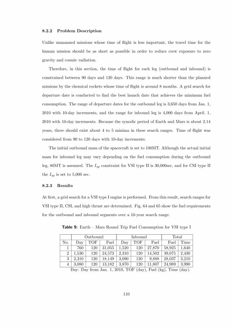
8.2.2 Problem Description
Unlike unmanned missions whose time of flight is less important, the travel time for the
human mission should be as short as possible in order to reduce crew exposure to zero
gravity and cosmic radiation.
Therefore, in this section, the time of flight for each leg (outbound and inbound) is
constrained between 90 days and 120 days. This range is much shorter than the planned
missions by the chemical rockets whose time of flight is around 8 months. A grid search for
departure date is conducted to find the best launch date that achieves the minimum fuel
consumption. The range of departure dates for the outbound leg is 3,650 days from Jan. 1,
2010 with 10-day increments, and the range for inbound leg is 4,000 days from April. 1,
2010 with 10-day increments. Because the synodic period of Earth and Mars is about 2.14
years, there should exist about 4 to 5 minima in these search ranges. Time of flight was
considered from 90 to 120 days with 10-day increments.
The initial outbound mass of the spacecraft is set to 100MT. Although the actual initial
mass for inbound leg may vary depending on the fuel consumption during the outbound
leg, 80MT is assumed. The Isp constraint for VSI type II is 30,000sec, and for CSI type II
the Isp is set to 5,000 sec.
8.2.3 Results
At first, a grid search for a VSI type I engine is performed. From this result, search ranges for
VSI type II, CSI, and high thrust are determined. Fig. 64 and 65 show the fuel requirements
for the outbound and inbound segments over a 10-year search range.
Table 9: Earth – Mars Round Trip Fuel Consumption for VSI type I
Outbound Inbound Total
No. Day TOF Fuel Day TOF Fuel Fuel Time
1 760 120 31,055 1,520 120 27,870 58,925 1,640
2 1,530 120 24,573 2,310 120 14,502 39,075 2,430
3 2,310 120 18,149 3,090 120 9,888 28,037 3,210
4 3,080 120 13,182 3,870 120 11,807 24,989 3,990
Day: Day from Jan. 1, 2010, TOF (day), Fuel (kg), Time (day).
110
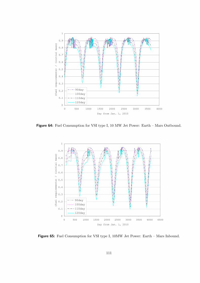
0
0.1
0.2
0.3
0.4
0.5
0.6
0.7
0.8
0.9
1
0 500 1000 1500 2000 2500 3000 3500 4000
Day from Jan. 1, 2010
(fuel requirements) / (initial mass)
90day
100day
110day
120day
Figure 64: Fuel Consumption for VSI type I, 10 MW Jet Power: Earth – Mars Outbound.
0
0.1
0.2
0.3
0.4
0.5
0.6
0.7
0.8
0.9
1
0 500 1000 1500 2000 2500 3000 3500 4000 4500
Day from Jan. 1, 2010
(fuel requirements) / (initial mass)
90day
100day
110day
120day
Figure 65: Fuel Consumption for VSI type I, 10MW Jet Power: Earth – Mars Inbound.
111
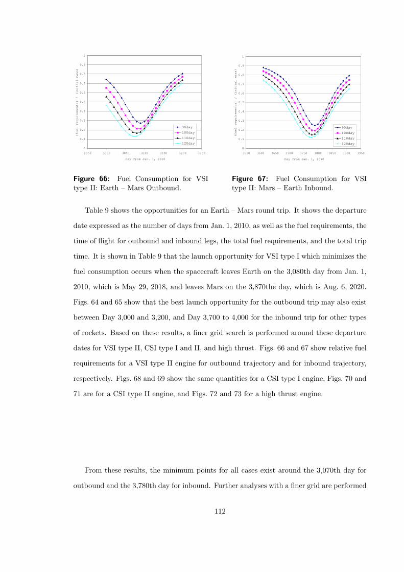
0
0.1
0.2
0.3
0.4
0.5
0.6
0.7
0.8
0.9
1
2950 3000 3050 3100 3150 3200 3250
Day from Jan. 1, 2010
(fuel requirements) / (initial mass)
90day
100day
110day
120day
Figure 66: Fuel Consumption for VSItype II: Earth – Mars Outbound.
0
0.1
0.2
0.3
0.4
0.5
0.6
0.7
0.8
0.9
1
3550 3600 3650 3700 3750 3800 3850 3900 3950
Day from Jan. 1, 2010
(fuel requirements) / (initial mass)
90day
100day
110day
120day
Figure 67: Fuel Consumption for VSItype II: Mars – Earth Inbound.
Table 9 shows the opportunities for an Earth – Mars round trip. It shows the departure
date expressed as the number of days from Jan. 1, 2010, as well as the fuel requirements, the
time of flight for outbound and inbound legs, the total fuel requirements, and the total trip
time. It is shown in Table 9 that the launch opportunity for VSI type I which minimizes the
fuel consumption occurs when the spacecraft leaves Earth on the 3,080th day from Jan. 1,
2010, which is May 29, 2018, and leaves Mars on the 3,870the day, which is Aug. 6, 2020.
Figs. 64 and 65 show that the best launch opportunity for the outbound trip may also exist
between Day 3,000 and 3,200, and Day 3,700 to 4,000 for the inbound trip for other types
of rockets. Based on these results, a finer grid search is performed around these departure
dates for VSI type II, CSI type I and II, and high thrust. Figs. 66 and 67 show relative fuel
requirements for a VSI type II engine for outbound trajectory and for inbound trajectory,
respectively. Figs. 68 and 69 show the same quantities for a CSI type I engine, Figs. 70 and
71 are for a CSI type II engine, and Figs. 72 and 73 for a high thrust engine.
From these results, the minimum points for all cases exist around the 3,070th day for
outbound and the 3,780th day for inbound. Further analyses with a finer grid are performed
112
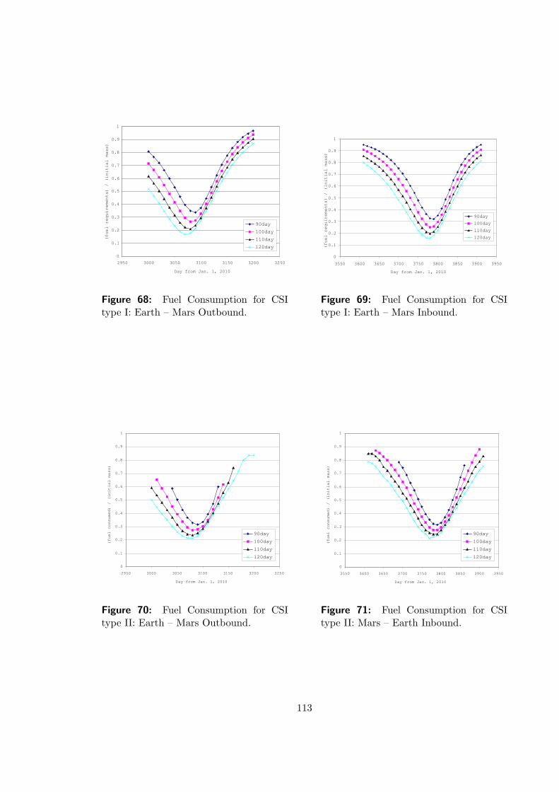
0
0.1
0.2
0.3
0.4
0.5
0.6
0.7
0.8
0.9
1
2950 3000 3050 3100 3150 3200 3250
Day from Jan. 1, 2010
(fuel requirements) / (initial mass)
90day
100day
110day
120day
Figure 68: Fuel Consumption for CSItype I: Earth – Mars Outbound.
0
0.1
0.2
0.3
0.4
0.5
0.6
0.7
0.8
0.9
1
3550 3600 3650 3700 3750 3800 3850 3900 3950
Day from Jan. 1, 2010
(fuel requirements) / (initial mass)
90day
100day
110day
120day
Figure 69: Fuel Consumption for CSItype I: Earth – Mars Inbound.
0
0.1
0.2
0.3
0.4
0.5
0.6
0.7
0.8
0.9
1
2950 3000 3050 3100 3150 3200 3250
Day from Jan. 1, 2010
(fuel consumed) / (initial mass)
90day
100day
110day
120day
Figure 70: Fuel Consumption for CSItype II: Earth – Mars Outbound.
0
0.1
0.2
0.3
0.4
0.5
0.6
0.7
0.8
0.9
1
3550 3600 3650 3700 3750 3800 3850 3900 3950
Day from Jan. 1, 2010
(fuel consumed) / (initial mass)
90day
100day
110day
120day
Figure 71: Fuel Consumption for CSItype II: Mars – Earth Inbound.
113
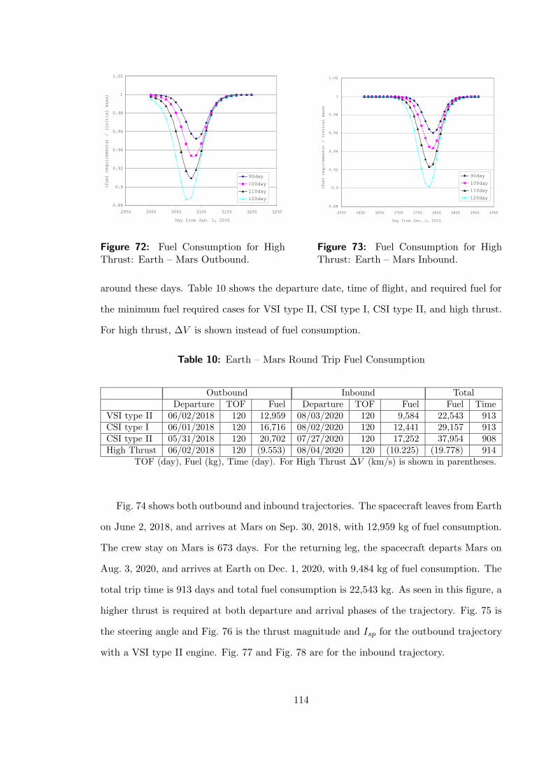
0.88
0.9
0.92
0.94
0.96
0.98
1
1.02
2950 3000 3050 3100 3150 3200 3250
Day from Jan. 1, 2010
(fuel requirements) / (initial mass)
90day
100day
110day
120day
Figure 72: Fuel Consumption for HighThrust: Earth – Mars Outbound.
0.88
0.9
0.92
0.94
0.96
0.98
1
1.02
3550 3600 3650 3700 3750 3800 3850 3900 3950
Day from Jan. 1, 2010
(fuel requirements) / (initial mass)
90day
100day
110day
120day
Figure 73: Fuel Consumption for HighThrust: Earth – Mars Inbound.
around these days. Table 10 shows the departure date, time of flight, and required fuel for
the minimum fuel required cases for VSI type II, CSI type I, CSI type II, and high thrust.
For high thrust, ∆V is shown instead of fuel consumption.
Table 10: Earth – Mars Round Trip Fuel Consumption
Outbound Inbound TotalDeparture TOF Fuel Departure TOF Fuel Fuel Time
VSI type II 06/02/2018 120 12,959 08/03/2020 120 9,584 22,543 913CSI type I 06/01/2018 120 16,716 08/02/2020 120 12,441 29,157 913CSI type II 05/31/2018 120 20,702 07/27/2020 120 17,252 37,954 908High Thrust 06/02/2018 120 (9.553) 08/04/2020 120 (10.225) (19.778) 914
TOF (day), Fuel (kg), Time (day). For High Thrust ∆V (km/s) is shown in parentheses.
Fig. 74 shows both outbound and inbound trajectories. The spacecraft leaves from Earth
on June 2, 2018, and arrives at Mars on Sep. 30, 2018, with 12,959 kg of fuel consumption.
The crew stay on Mars is 673 days. For the returning leg, the spacecraft departs Mars on
Aug. 3, 2020, and arrives at Earth on Dec. 1, 2020, with 9,484 kg of fuel consumption. The
total trip time is 913 days and total fuel consumption is 22,543 kg. As seen in this figure, a
higher thrust is required at both departure and arrival phases of the trajectory. Fig. 75 is
the steering angle and Fig. 76 is the thrust magnitude and Isp for the outbound trajectory
with a VSI type II engine. Fig. 77 and Fig. 78 are for the inbound trajectory.
114
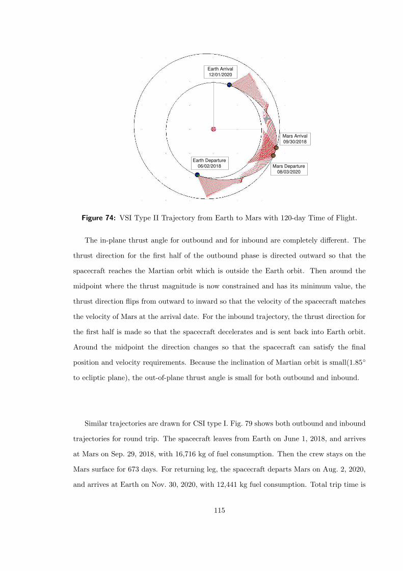
Earth Departure 06/02/2018
Mars Arrival 09/30/2018
Mars Departure 08/03/2020
Earth Arrival 12/01/2020
Figure 74: VSI Type II Trajectory from Earth to Mars with 120-day Time of Flight.
The in-plane thrust angle for outbound and for inbound are completely different. The
thrust direction for the first half of the outbound phase is directed outward so that the
spacecraft reaches the Martian orbit which is outside the Earth orbit. Then around the
midpoint where the thrust magnitude is now constrained and has its minimum value, the
thrust direction flips from outward to inward so that the velocity of the spacecraft matches
the velocity of Mars at the arrival date. For the inbound trajectory, the thrust direction for
the first half is made so that the spacecraft decelerates and is sent back into Earth orbit.
Around the midpoint the direction changes so that the spacecraft can satisfy the final
position and velocity requirements. Because the inclination of Martian orbit is small(1.85
to ecliptic plane), the out-of-plane thrust angle is small for both outbound and inbound.
Similar trajectories are drawn for CSI type I. Fig. 79 shows both outbound and inbound
trajectories for round trip. The spacecraft leaves from Earth on June 1, 2018, and arrives
at Mars on Sep. 29, 2018, with 16,716 kg of fuel consumption. Then the crew stays on the
Mars surface for 673 days. For returning leg, the spacecraft departs Mars on Aug. 2, 2020,
and arrives at Earth on Nov. 30, 2020, with 12,441 kg fuel consumption. Total trip time is
115
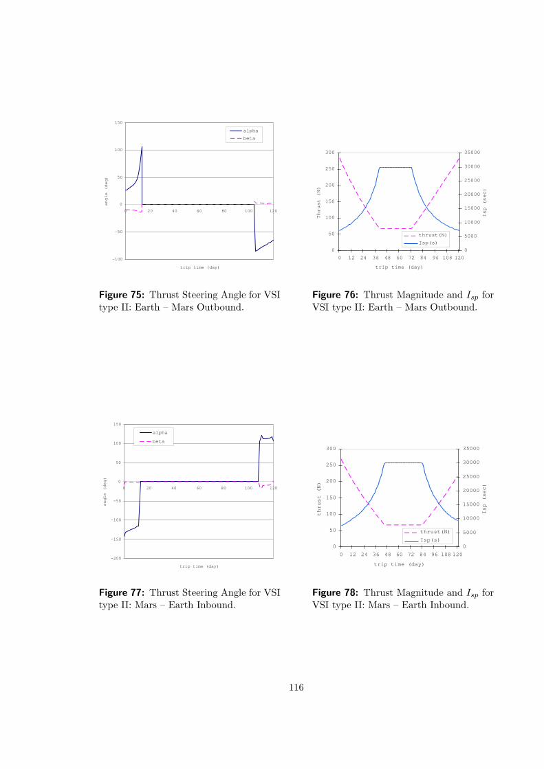
-100
-50
0
50
100
150
0 20 40 60 80 100 120
trip time (day)
angle (deg)
alpha
beta
Figure 75: Thrust Steering Angle for VSItype II: Earth – Mars Outbound.
0
50
100
150
200
250
300
0 12 24 36 48 60 72 84 96 108 120
trip time (day)
Thrust (N)
0
5000
10000
15000
20000
25000
30000
35000
Isp (sec)
thrust(N)
Isp(s)
Figure 76: Thrust Magnitude and Isp forVSI type II: Earth – Mars Outbound.
-200
-150
-100
-50
0
50
100
150
0 20 40 60 80 100 120
trip time (day)
angle (deg)
alpha
beta
Figure 77: Thrust Steering Angle for VSItype II: Mars – Earth Inbound.
0
50
100
150
200
250
300
0 12 24 36 48 60 72 84 96 108 120
trip time (day)
thrust (N)
0
5000
10000
15000
20000
25000
30000
35000
Isp (sec)
thrust(N)
Isp(s)
Figure 78: Thrust Magnitude and Isp forVSI type II: Mars – Earth Inbound.
116
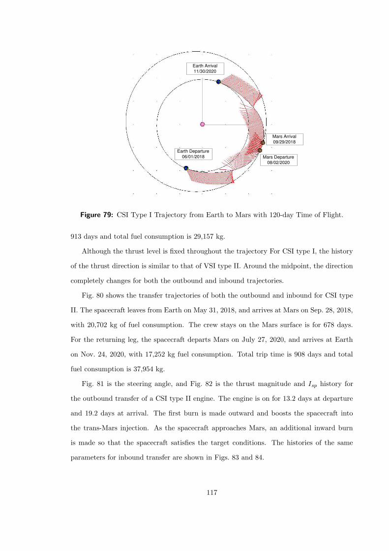
Earth Departure 06/01/2018 Mars Departure
08/02/2020
Mars Arrival 09/29/2018
Earth Arrival 11/30/2020
Figure 79: CSI Type I Trajectory from Earth to Mars with 120-day Time of Flight.
913 days and total fuel consumption is 29,157 kg.
Although the thrust level is fixed throughout the trajectory For CSI type I, the history
of the thrust direction is similar to that of VSI type II. Around the midpoint, the direction
completely changes for both the outbound and inbound trajectories.
Fig. 80 shows the transfer trajectories of both the outbound and inbound for CSI type
II. The spacecraft leaves from Earth on May 31, 2018, and arrives at Mars on Sep. 28, 2018,
with 20,702 kg of fuel consumption. The crew stays on the Mars surface is for 678 days.
For the returning leg, the spacecraft departs Mars on July 27, 2020, and arrives at Earth
on Nov. 24, 2020, with 17,252 kg fuel consumption. Total trip time is 908 days and total
fuel consumption is 37,954 kg.
Fig. 81 is the steering angle, and Fig. 82 is the thrust magnitude and Isp history for
the outbound transfer of a CSI type II engine. The engine is on for 13.2 days at departure
and 19.2 days at arrival. The first burn is made outward and boosts the spacecraft into
the trans-Mars injection. As the spacecraft approaches Mars, an additional inward burn
is made so that the spacecraft satisfies the target conditions. The histories of the same
parameters for inbound transfer are shown in Figs. 83 and 84.
117
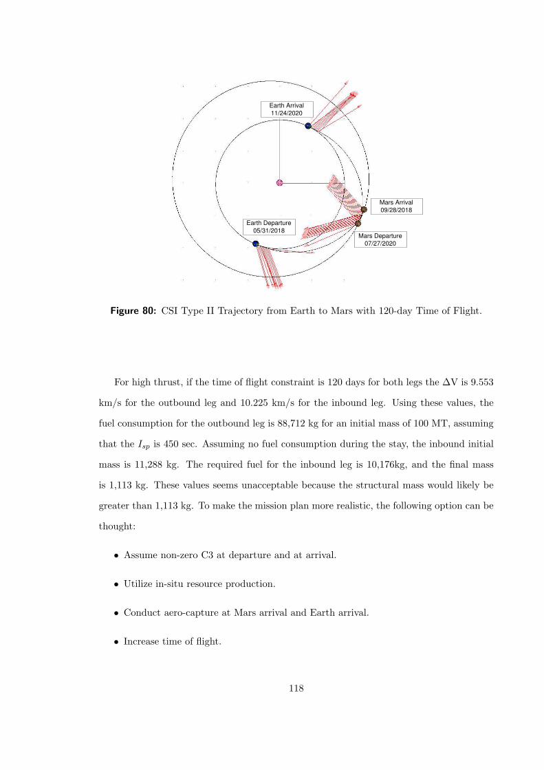
Earth Departure 05/31/2018
Mars Departure 07/27/2020
Mars Arrival 09/28/2018
Earth Arrival 11/14/2020 Earth Arrival 11/24/2020
Figure 80: CSI Type II Trajectory from Earth to Mars with 120-day Time of Flight.
For high thrust, if the time of flight constraint is 120 days for both legs the ∆V is 9.553
km/s for the outbound leg and 10.225 km/s for the inbound leg. Using these values, the
fuel consumption for the outbound leg is 88,712 kg for an initial mass of 100 MT, assuming
that the Isp is 450 sec. Assuming no fuel consumption during the stay, the inbound initial
mass is 11,288 kg. The required fuel for the inbound leg is 10,176kg, and the final mass
is 1,113 kg. These values seems unacceptable because the structural mass would likely be
greater than 1,113 kg. To make the mission plan more realistic, the following option can be
thought:
• Assume non-zero C3 at departure and at arrival.
• Utilize in-situ resource production.
• Conduct aero-capture at Mars arrival and Earth arrival.
• Increase time of flight.
118
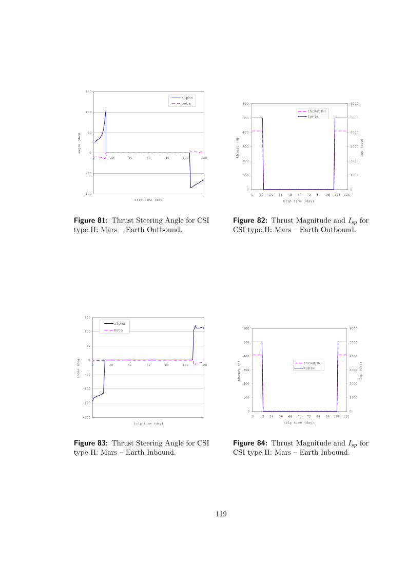
-100
-50
0
50
100
150
0 20 40 60 80 100 120
trip time (day)
angle (deg)
alpha
beta
Figure 81: Thrust Steering Angle for CSItype II: Mars – Earth Outbound.
0
100
200
300
400
500
600
0 12 24 36 48 60 72 84 96 108 120
trip time (day)
thrust (N)
0
1000
2000
3000
4000
5000
6000
Isp (sec)
thrust(N)
Isp(s)
Figure 82: Thrust Magnitude and Isp forCSI type II: Mars – Earth Outbound.
-200
-150
-100
-50
0
50
100
150
0 20 40 60 80 100 120
trip time (day)
angle (deg)
alpha
beta
Figure 83: Thrust Steering Angle for CSItype II: Mars – Earth Inbound.
0
100
200
300
400
500
600
0 12 24 36 48 60 72 84 96 108 120
trip time (day)
thrust (N)
0
1000
2000
3000
4000
5000
6000
Isp (sec)
thrust(N)
Isp(s)
Figure 84: Thrust Magnitude and Isp forCSI type II: Mars – Earth Inbound.
119
In reality the spacecraft usually has some non-zero value of C3. If a spacecraft leaves
LEO and heads to Mars it should have some velocity when it escapes from the Earth’s
sphere of influence.
In-situ resource utilization is the process of using the materials available in the environ-
ment. For a Mars mission, this typically refers to using atmospheric materials to make fuel.
Mars has an atmosphere of 95% carbon dioxide, or CO2, and can be reacted directly with
the hydrogen brought from Earth as: 3CO2 + 6H2 → CH4 + 2CO + 4H2O. If the water
obtained from this reaction is run through a simple electrolysis process, i.e.: 2H2O → 2H2
+ O2, the hydrogen trapped in the water as a result of the first equation can be brought
back to product more and more methane, with a large amount of oxygen being produced
that could serve as a backup to the life-supporting systems of the Mars habitat.
Aero-capture could also be used to capture into Earth and Mars orbit, this could help
decrease the fuel requirements. The possibility of aero-capture is not analyzed in this
research.
Finally, to explore the possibility of saving the fuel by increasing the time of flight, a
broader range for time of flight is searched. The search range is now 100 to 400 days for both
legs. The minimum fuel transfer is achieved when the spacecraft leaves Earth on May 1,
2018, and arrives at Mars on Nov. 17, 2018, and then leaves Mars on June 29, 2020, and
arrives at Earth on Jan. 5, 2021. The time of flight is 200 days for the outbound leg and 190
days for the inbound leg. The ∆V for the outbound leg is 6.013 km/sec, and 6.810 km/sec
for the inbound leg. The fuel consumption for the outbound leg is 74,403 kg, and if no fuel
is consumed during the stay, then the initial inbound mass is 25,597 kg. The inbound leg
requires 20,127 kg of fuel, and gives a final mass of 5,470 kg. If other techniques introduced
above are used, the fuel consumption could be lowered.
120
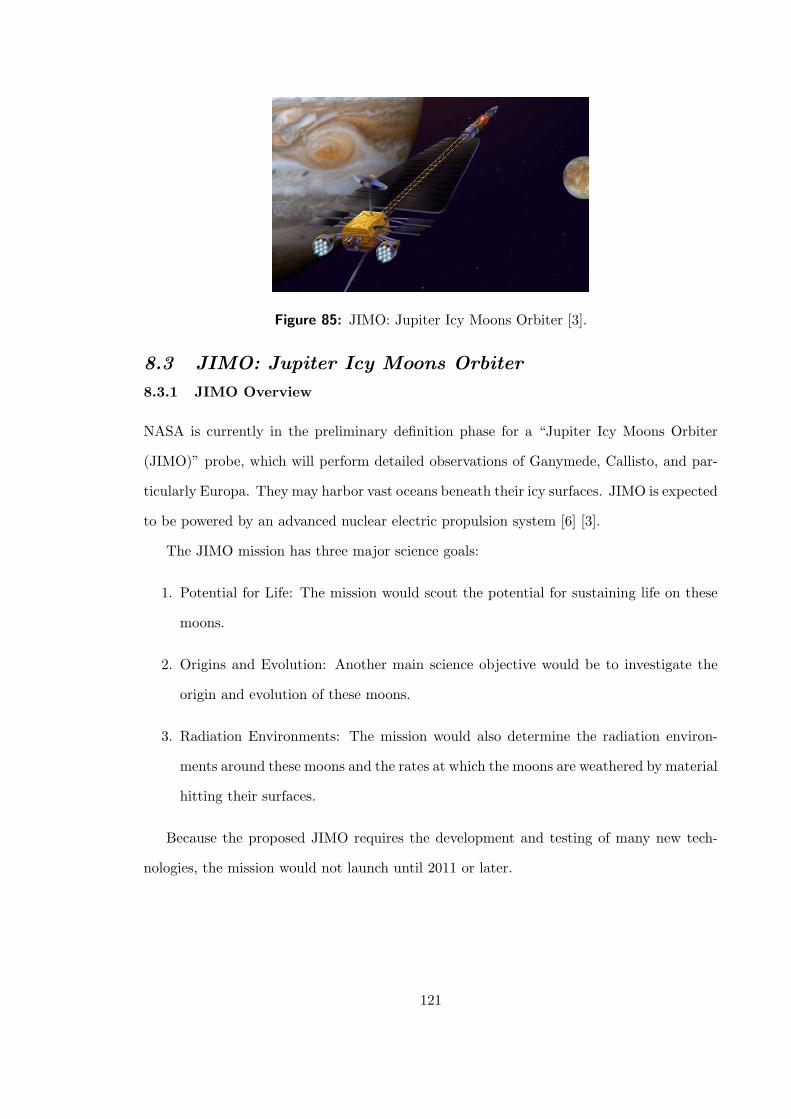
Figure 85: JIMO: Jupiter Icy Moons Orbiter [3].
8.3 JIMO: Jupiter Icy Moons Orbiter
8.3.1 JIMO Overview
NASA is currently in the preliminary definition phase for a “Jupiter Icy Moons Orbiter
(JIMO)” probe, which will perform detailed observations of Ganymede, Callisto, and par-
ticularly Europa. They may harbor vast oceans beneath their icy surfaces. JIMO is expected
to be powered by an advanced nuclear electric propulsion system [6] [3].
The JIMO mission has three major science goals:
1. Potential for Life: The mission would scout the potential for sustaining life on these
moons.
2. Origins and Evolution: Another main science objective would be to investigate the
origin and evolution of these moons.
3. Radiation Environments: The mission would also determine the radiation environ-
ments around these moons and the rates at which the moons are weathered by material
hitting their surfaces.
Because the proposed JIMO requires the development and testing of many new tech-
nologies, the mission would not launch until 2011 or later.
121

0
40
80
120
160
200
240
280
320
360
400 300
750
0
0.1
0.2
0.3
0.4
0.5
0.6
0.7
0.8
0.9
1
(fuel consumed) / (initial
mass)
Day from Jan. 1, 2010 TOF
(day)
Figure 86: Fuel Consumption for VSI type I: Earth – Jupiter.
8.3.2 Problem Description
The synodic period of Earth and Jupiter is 398.9 days. The fuel requirements for a 400-day
range of departure dates are searched starting from Jan. 1, 2010. Initially, a wide range of
time of flight was considered, and then from the results, an appropriate value of time of
flight was chosen and a more precise analyses could be conducted.
For this section, an upper Isp limit for CSI type I is set to 30,000 sec. The Isp limit for
VSI type II is the same as the last sections (30,000 sec), and Isp level for CSI type II is
5,000 sec.
8.3.3 Results
The trajectory for a VSI type I engine was analyzed to narrow the search range. Fig. 86
shows the fuel requirements for a transfer from Earth to Jupiter. The minimum-fuel transfer
occurs when the spacecraft departs around 100 days after Jan. 1, 2010. A more precise
analysis is performed around these days for VSI type II, CSI type I and II, and high thrust.
Fig. 87 shows the fuel requirements for an Earth to Jupiter transfer with VSI type II for
122
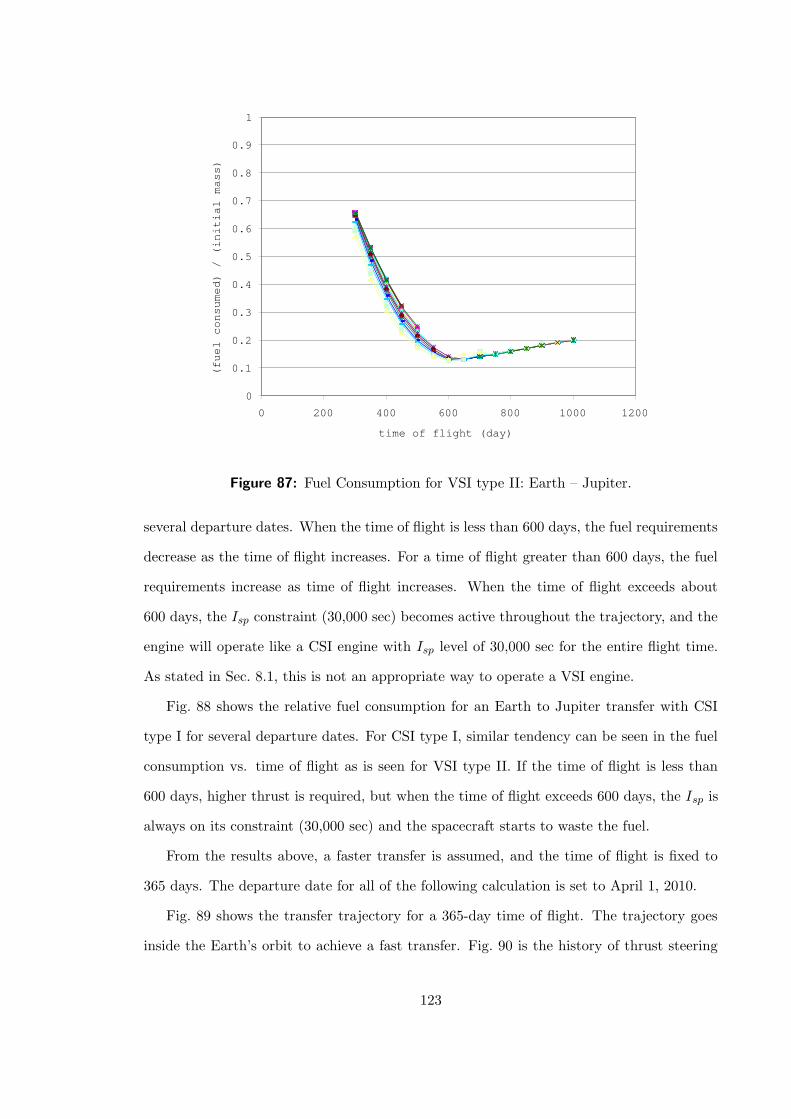
0
0.1
0.2
0.3
0.4
0.5
0.6
0.7
0.8
0.9
1
0 200 400 600 800 1000 1200
time of flight (day)
(fuel consumed) / (initial mass)
Figure 87: Fuel Consumption for VSI type II: Earth – Jupiter.
several departure dates. When the time of flight is less than 600 days, the fuel requirements
decrease as the time of flight increases. For a time of flight greater than 600 days, the fuel
requirements increase as time of flight increases. When the time of flight exceeds about
600 days, the Isp constraint (30,000 sec) becomes active throughout the trajectory, and the
engine will operate like a CSI engine with Isp level of 30,000 sec for the entire flight time.
As stated in Sec. 8.1, this is not an appropriate way to operate a VSI engine.
Fig. 88 shows the relative fuel consumption for an Earth to Jupiter transfer with CSI
type I for several departure dates. For CSI type I, similar tendency can be seen in the fuel
consumption vs. time of flight as is seen for VSI type II. If the time of flight is less than
600 days, higher thrust is required, but when the time of flight exceeds 600 days, the Isp is
always on its constraint (30,000 sec) and the spacecraft starts to waste the fuel.
From the results above, a faster transfer is assumed, and the time of flight is fixed to
365 days. The departure date for all of the following calculation is set to April 1, 2010.
Fig. 89 shows the transfer trajectory for a 365-day time of flight. The trajectory goes
inside the Earth’s orbit to achieve a fast transfer. Fig. 90 is the history of thrust steering
123
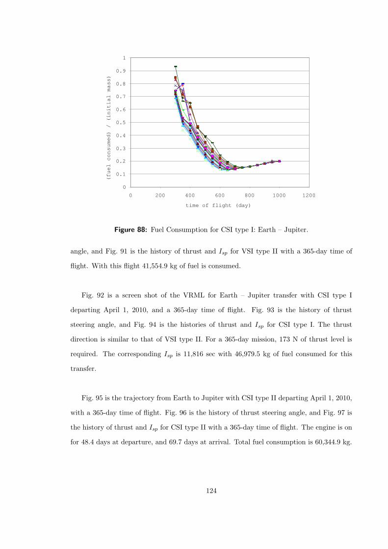
0
0.1
0.2
0.3
0.4
0.5
0.6
0.7
0.8
0.9
1
0 200 400 600 800 1000 1200
time of flight (day)
(fuel consumed) / (initial mass)
Figure 88: Fuel Consumption for CSI type I: Earth – Jupiter.
angle, and Fig. 91 is the history of thrust and Isp for VSI type II with a 365-day time of
flight. With this flight 41,554.9 kg of fuel is consumed.
Fig. 92 is a screen shot of the VRML for Earth – Jupiter transfer with CSI type I
departing April 1, 2010, and a 365-day time of flight. Fig. 93 is the history of thrust
steering angle, and Fig. 94 is the histories of thrust and Isp for CSI type I. The thrust
direction is similar to that of VSI type II. For a 365-day mission, 173 N of thrust level is
required. The corresponding Isp is 11,816 sec with 46,979.5 kg of fuel consumed for this
transfer.
Fig. 95 is the trajectory from Earth to Jupiter with CSI type II departing April 1, 2010,
with a 365-day time of flight. Fig. 96 is the history of thrust steering angle, and Fig. 97 is
the history of thrust and Isp for CSI type II with a 365-day time of flight. The engine is on
for 48.4 days at departure, and 69.7 days at arrival. Total fuel consumption is 60,344.9 kg.
124
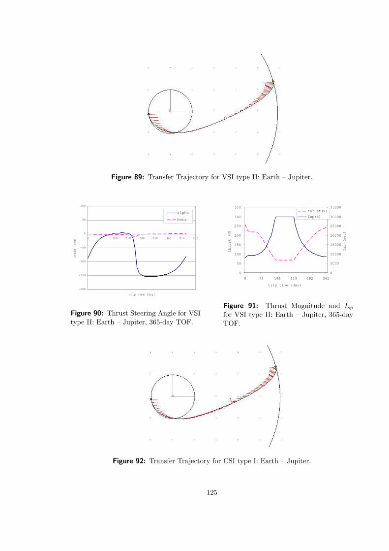
Figure 89: Transfer Trajectory for VSI type II: Earth – Jupiter.
-200
-150
-100
-50
0
50
100
0 50 100 150 200 250 300 350 400
trip time (day)
angle (deg)
alpha
beta
Figure 90: Thrust Steering Angle for VSItype II: Earth – Jupiter, 365-day TOF.
0
50
100
150
200
250
300
350
0 73 146 219 292 365
trip time (day)
thrust (N)
0
5000
10000
15000
20000
25000
30000
35000
Isp (sec)
thrust(N)
Isp(s)
Figure 91: Thrust Magnitude and Ispfor VSI type II: Earth – Jupiter, 365-dayTOF.
Figure 92: Transfer Trajectory for CSI type I: Earth – Jupiter.
125
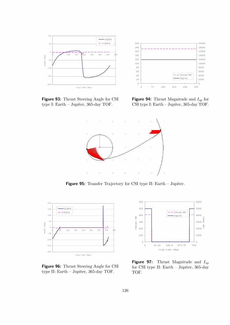
-200
-150
-100
-50
0
50
100
0 50 100 150 200 250 300 350 400
trip time (day)
angle (deg)
alpha
beta
Figure 93: Thrust Steering Angle for CSItype I: Earth – Jupiter, 365-day TOF.
0
20
40
60
80
100
120
140
160
180
200
0 73 146 219 292 365
0
2000
4000
6000
8000
10000
12000
14000
16000
18000
20000
thrust(N)
Isp(s)
Figure 94: Thrust Magnitude and Isp forCSI type I: Earth – Jupiter, 365-day TOF.
Figure 95: Transfer Trajectory for CSI type II: Earth – Jupiter.
-200
-150
-100
-50
0
50
100
150
200
0 50 100 150 200 250 300 350 400
trip time (day)
angle (deg)
alpha
beta
Figure 96: Thrust Steering Angle for CSItype II: Earth – Jupiter, 365-day TOF.
0
100
200
300
400
500
600
0 91.25 182.5 273.75 365
trip time (day)
thrust (N)
0
1000
2000
3000
4000
5000
6000 Isp (sec)
thrust(N)
Isp(s)
Figure 97: Thrust Magnitude and Ispfor CSI type II: Earth – Jupiter, 365-dayTOF.
126

8.4 Uranus and beyond
A transfer orbit to planets such as Uranus, Neptune, and Pluto, the launch opportunity
comes about once a year because the synodic period for Earth and these planets is about
one year. In this section a transfer trajectory from Earth to Uranus is analyzed. Transfer
trajectories to other two planets should be similar.
One thing we should remember in computing a transfer trajectory to the planet far
from the Sun is that as the transfer time gets longer, we need to think about the maximum
allowable burn time. Consider a spacecraft with 100 MT (1.0E+05 kg) of initial fuel and a a
VSI type II engine with a 30,000 sec Isp limit. If the jet power is 30 MW the propellant mass
flow becomes mprop = 2PJ/(g0 · Isp)2 = 6.933E-04 kg/s. Then it takes 1.0E+05/6.9334E-04
= 1.4424E+08 sec = 1669.4 days = 4.57 years until the spacecraft mass becomes zero. For
a jet power of 10 MW, 5008.2 days or 13.712 years is the time limit. We should reach the
target planet at least by then. For a CSI type II engine with 10 MW jet power and 5,000
sec Isp, mprop is 8.3197E-03 kg/s, and the burn time should be less than 139.1 days.
A grid search for a 400-day range of departure date from Jan. 1, 2010, is conducted for
VSI type I engine. The time of flight is fixed to 1,000 days. The minimum fuel trajectory
is achieved when the spacecraft is launched on Aug. 28, 2010. Using this launch date and
a 1,000-day time of flight, transfer trajectories for VSI type II, CSI type I, and CSI type II
are calculated.
Figs. 98 to 103 show the transfer trajectories from Earth to Uranus with 1,000-day time
of flight. 10MW of jet power is powerful enough to get the spacecraft to Uranus within
the 1,000-day limit. For these types of engines, the trajectory is almost straight to Uranus.
Fuel requirements are: 36,361.9 kg for VSI type II, 46,514.0 kg for CSI type I, 69006.7 kg
for CSI type II. The thrust level for CSI type I is 103.8 N (corresponding Isp is 19,656 sec),
and burn time for CSI type II is 94 days (54 days at departure, 40 days at arrival).
127

Figure 98: Transfer Trajectory for VSItype II: Earth – Uranus.
Figure 99: Departure Phase of Trans-fer Trajectory for VSI type II: Earth –Uranus.
Figure 100: Transfer Trajectory for CSItype I: Earth – Uranus.
Figure 101: Departure Phase of TransferTrajectory for CSI type I: Earth – Uranus.
128
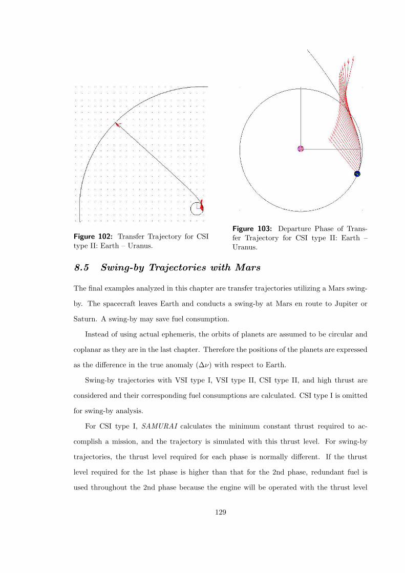
Figure 102: Transfer Trajectory for CSItype II: Earth – Uranus.
Figure 103: Departure Phase of Trans-fer Trajectory for CSI type II: Earth –Uranus.
8.5 Swing-by Trajectories with Mars
The final examples analyzed in this chapter are transfer trajectories utilizing a Mars swing-
by. The spacecraft leaves Earth and conducts a swing-by at Mars en route to Jupiter or
Saturn. A swing-by may save fuel consumption.
Instead of using actual ephemeris, the orbits of planets are assumed to be circular and
coplanar as they are in the last chapter. Therefore the positions of the planets are expressed
as the difference in the true anomaly (∆ν) with respect to Earth.
Swing-by trajectories with VSI type I, VSI type II, CSI type II, and high thrust are
considered and their corresponding fuel consumptions are calculated. CSI type I is omitted
for swing-by analysis.
For CSI type I, SAMURAI calculates the minimum constant thrust required to ac-
complish a mission, and the trajectory is simulated with this thrust level. For swing-by
trajectories, the thrust level required for each phase is normally different. If the thrust
level required for the 1st phase is higher than that for the 2nd phase, redundant fuel is
used throughout the 2nd phase because the engine will be operated with the thrust level
129
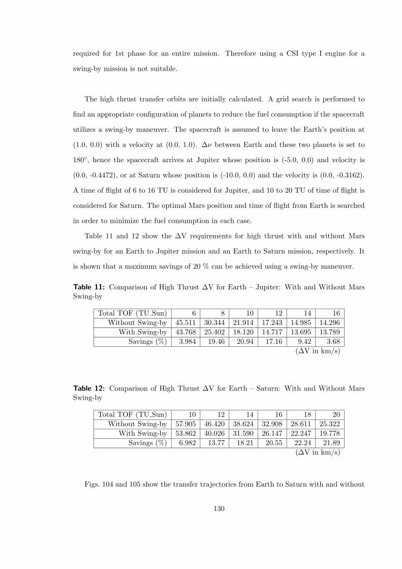
required for 1st phase for an entire mission. Therefore using a CSI type I engine for a
swing-by mission is not suitable.
The high thrust transfer orbits are initially calculated. A grid search is performed to
find an appropriate configuration of planets to reduce the fuel consumption if the spacecraft
utilizes a swing-by maneuver. The spacecraft is assumed to leave the Earth’s position at
(1.0, 0.0) with a velocity at (0.0, 1.0). ∆ν between Earth and these two planets is set to
180, hence the spacecraft arrives at Jupiter whose position is (-5.0, 0.0) and velocity is
(0.0, -0.4472), or at Saturn whose position is (-10.0, 0.0) and the velocity is (0.0, -0.3162).
A time of flight of 6 to 16 TU is considered for Jupiter, and 10 to 20 TU of time of flight is
considered for Saturn. The optimal Mars position and time of flight from Earth is searched
in order to minimize the fuel consumption in each case.
Table 11 and 12 show the ∆V requirements for high thrust with and without Mars
swing-by for an Earth to Jupiter mission and an Earth to Saturn mission, respectively. It
is shown that a maximum savings of 20 % can be achieved using a swing-by maneuver.
Table 11: Comparison of High Thrust ∆V for Earth – Jupiter: With and Without MarsSwing-by
Total TOF (TU Sun) 6 8 10 12 14 16
Without Swing-by 45.511 30.344 21.914 17.243 14.985 14.296
With Swing-by 43.768 25.402 18.120 14.717 13.695 13.789
Savings (%) 3.984 19.46 20.94 17.16 9.42 3.68
(∆V in km/s)
Table 12: Comparison of High Thrust ∆V for Earth – Saturn: With and Without MarsSwing-by
Total TOF (TU Sun) 10 12 14 16 18 20
Without Swing-by 57.905 46.420 38.624 32.908 28.611 25.322
With Swing-by 53.862 40.026 31.590 26.147 22.247 19.778
Savings (%) 6.982 13.77 18.21 20.55 22.24 21.89
(∆V in km/s)
Figs. 104 and 105 show the transfer trajectories from Earth to Saturn with and without
130
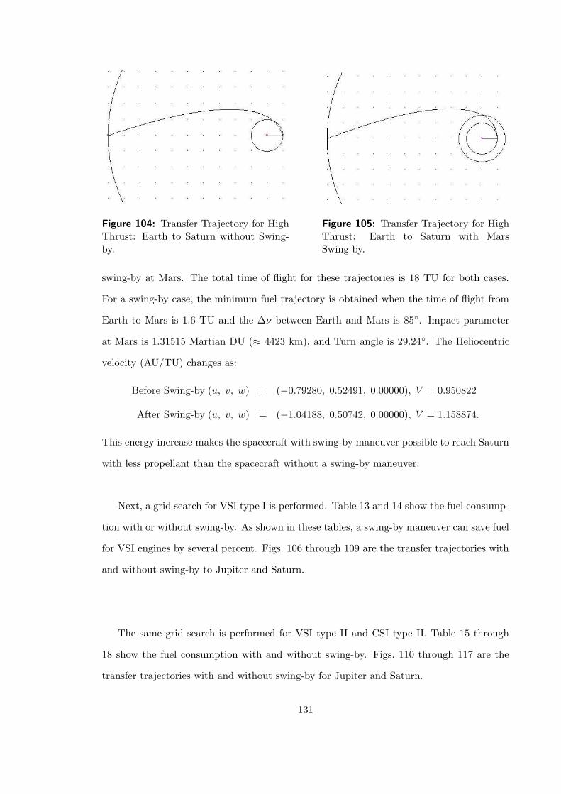
Figure 104: Transfer Trajectory for HighThrust: Earth to Saturn without Swing-by.
Figure 105: Transfer Trajectory for HighThrust: Earth to Saturn with MarsSwing-by.
swing-by at Mars. The total time of flight for these trajectories is 18 TU for both cases.
For a swing-by case, the minimum fuel trajectory is obtained when the time of flight from
Earth to Mars is 1.6 TU and the ∆ν between Earth and Mars is 85. Impact parameter
at Mars is 1.31515 Martian DU (≈ 4423 km), and Turn angle is 29.24. The Heliocentric
velocity (AU/TU) changes as:
Before Swing-by (u, v, w) = (−0.79280, 0.52491, 0.00000), V = 0.950822
After Swing-by (u, v, w) = (−1.04188, 0.50742, 0.00000), V = 1.158874.
This energy increase makes the spacecraft with swing-by maneuver possible to reach Saturn
with less propellant than the spacecraft without a swing-by maneuver.
Next, a grid search for VSI type I is performed. Table 13 and 14 show the fuel consump-
tion with or without swing-by. As shown in these tables, a swing-by maneuver can save fuel
for VSI engines by several percent. Figs. 106 through 109 are the transfer trajectories with
and without swing-by to Jupiter and Saturn.
The same grid search is performed for VSI type II and CSI type II. Table 15 through
18 show the fuel consumption with and without swing-by. Figs. 110 through 117 are the
transfer trajectories with and without swing-by for Jupiter and Saturn.
131
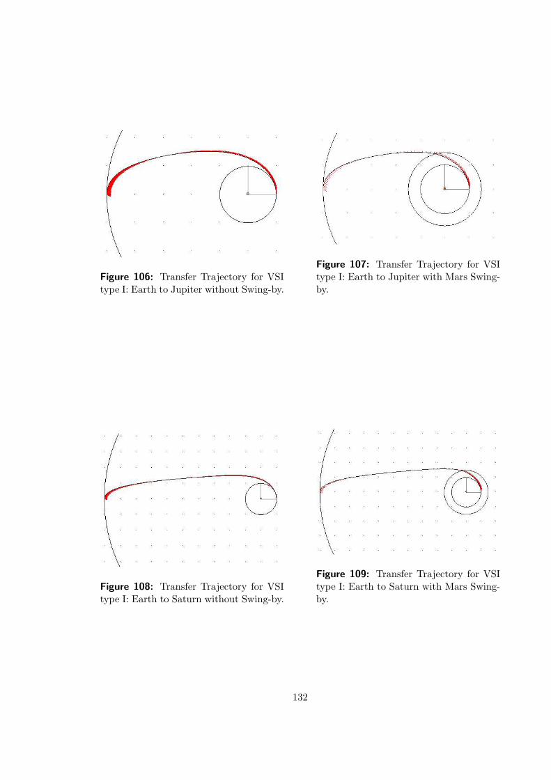
Figure 106: Transfer Trajectory for VSItype I: Earth to Jupiter without Swing-by.
Figure 107: Transfer Trajectory for VSItype I: Earth to Jupiter with Mars Swing-by.
Figure 108: Transfer Trajectory for VSItype I: Earth to Saturn without Swing-by.
Figure 109: Transfer Trajectory for VSItype I: Earth to Saturn with Mars Swing-by.
132
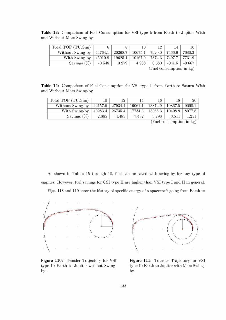
Table 13: Comparison of Fuel Consumption for VSI type I: from Earth to Jupiter Withand Without Mars Swing-by
Total TOF (TU Sun) 6 8 10 12 14 16
Without Swing-by 44764.1 20268.7 10675.1 7920.0 7466.6 7680.3
With Swing-by 45010.9 19625.1 10167.9 7874.3 7497.7 7731.9
Savings (%) -0.548 3.279 4.988 0.580 -0.415 -0.667
(Fuel consumption in kg)
Table 14: Comparison of Fuel Consumption for VSI type I: from Earth to Saturn Withand Without Mars Swing-by
Total TOF (TU Sun) 10 12 14 16 18 20
Without Swing-by 42157.6 27934.4 19061.1 13872.9 10867.5 9090.1
With Swing-by 40983.4 26735.4 17734.3 13365.3 10498.9 8977.8
Savings (%) 2.865 4.485 7.482 3.798 3.511 1.251
(Fuel consumption in kg)
As shown in Tables 15 through 18, fuel can be saved with swing-by for any type of
engines. However, fuel savings for CSI type II are higher than VSI type I and II in general.
Figs. 118 and 119 show the history of specific energy of a spacecraft going from Earth to
Figure 110: Transfer Trajectory for VSItype II: Earth to Jupiter without Swing-by.
Figure 111: Transfer Trajectory for VSItype II: Earth to Jupiter with Mars Swing-by.
133
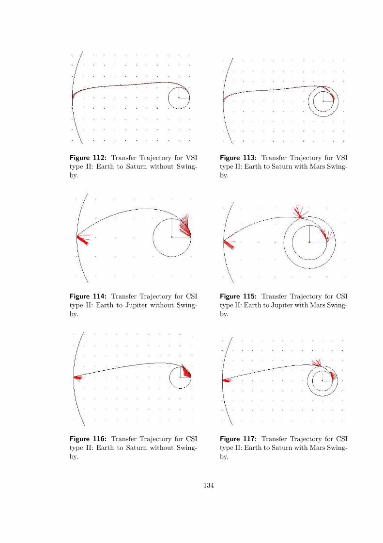
Figure 112: Transfer Trajectory for VSItype II: Earth to Saturn without Swing-by.
Figure 113: Transfer Trajectory for VSItype II: Earth to Saturn with Mars Swing-by.
Figure 114: Transfer Trajectory for CSItype II: Earth to Jupiter without Swing-by.
Figure 115: Transfer Trajectory for CSItype II: Earth to Jupiter with Mars Swing-by.
Figure 116: Transfer Trajectory for CSItype II: Earth to Saturn without Swing-by.
Figure 117: Transfer Trajectory for CSItype II: Earth to Saturn with Mars Swing-by.
134
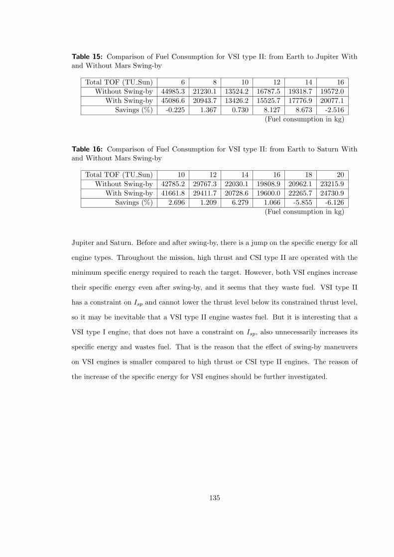
Table 15: Comparison of Fuel Consumption for VSI type II: from Earth to Jupiter Withand Without Mars Swing-by
Total TOF (TU Sun) 6 8 10 12 14 16
Without Swing-by 44985.3 21230.1 13524.2 16787.5 19318.7 19572.0
With Swing-by 45086.6 20943.7 13426.2 15525.7 17776.9 20077.1
Savings (%) -0.225 1.367 0.730 8.127 8.673 -2.516
(Fuel consumption in kg)
Table 16: Comparison of Fuel Consumption for VSI type II: from Earth to Saturn Withand Without Mars Swing-by
Total TOF (TU Sun) 10 12 14 16 18 20
Without Swing-by 42785.2 29767.3 22030.1 19808.9 20962.1 23215.9
With Swing-by 41661.8 29411.7 20728.6 19600.0 22265.7 24730.9
Savings (%) 2.696 1.209 6.279 1.066 -5.855 -6.126
(Fuel consumption in kg)
Jupiter and Saturn. Before and after swing-by, there is a jump on the specific energy for all
engine types. Throughout the mission, high thrust and CSI type II are operated with the
minimum specific energy required to reach the target. However, both VSI engines increase
their specific energy even after swing-by, and it seems that they waste fuel. VSI type II
has a constraint on Isp and cannot lower the thrust level below its constrained thrust level,
so it may be inevitable that a VSI type II engine wastes fuel. But it is interesting that a
VSI type I engine, that does not have a constraint on Isp, also unnecessarily increases its
specific energy and wastes fuel. That is the reason that the effect of swing-by maneuvers
on VSI engines is smaller compared to high thrust or CSI type II engines. The reason of
the increase of the specific energy for VSI engines should be further investigated.
135
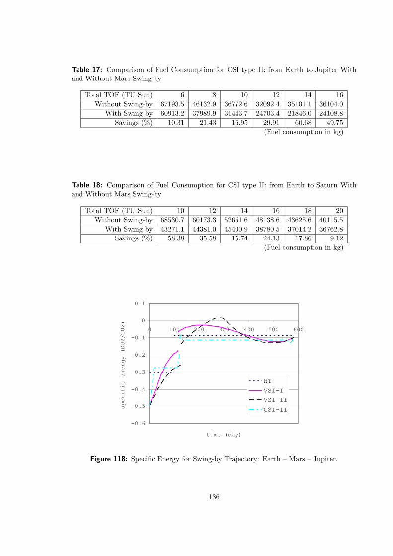
Table 17: Comparison of Fuel Consumption for CSI type II: from Earth to Jupiter Withand Without Mars Swing-by
Total TOF (TU Sun) 6 8 10 12 14 16
Without Swing-by 67193.5 46132.9 36772.6 32092.4 35101.1 36104.0
With Swing-by 60913.2 37989.9 31443.7 24703.4 21846.0 24108.8
Savings (%) 10.31 21.43 16.95 29.91 60.68 49.75
(Fuel consumption in kg)
Table 18: Comparison of Fuel Consumption for CSI type II: from Earth to Saturn Withand Without Mars Swing-by
Total TOF (TU Sun) 10 12 14 16 18 20
Without Swing-by 68530.7 60173.3 52651.6 48138.6 43625.6 40115.5
With Swing-by 43271.1 44381.0 45490.9 38780.5 37014.2 36762.8
Savings (%) 58.38 35.58 15.74 24.13 17.86 9.12
(Fuel consumption in kg)
-0.6
-0.5
-0.4
-0.3
-0.2
-0.1
0
0.1
0 100 200 300 400 500 600
time (day)
specific energy (DU2/TU2)
HT
VSI-I
VSI-II
CSI-II
Figure 118: Specific Energy for Swing-by Trajectory: Earth – Mars – Jupiter.
136
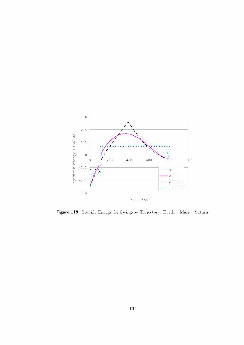
-0.6
-0.4
-0.2
0
0.2
0.4
0.6
0 200 400 600 800 1000
time (day)
specific energy (DU2/TU2)
HT
VSI-I
VSI-II
CSI-II
Figure 119: Specific Energy for Swing-by Trajectory: Earth – Mars – Saturn.
137
CHAPTER IX
CONCLUSIONS AND RECOMMENDED FUTURE
WORK
This paper has presented the methods and results for the comparison of several engine types
used for solar system exploration.
Five different engine types have been investigated in this research. They are
1. VSI type I (variable thrust, variable Isp with no constraint on Isp).
2. VSI type II (variable thrust, variable Isp with upper limit on Isp).
3. CSI type I (constant thrust, constant Isp with continuous thrust).
4. CSI type II (constant thrust, constant Isp with the capability of switching on/off the
engine).
5. High thrust (infinitesimal burn).
At first, a preliminary study was conducted with simple spiral trajectories, and fuel
consumption was calculated for VSI, CSI, and high thrust engines.
An interplanetary trajectory calculation software application SAMURAI was developed
to analyze the characteristics of trajectories for these five engines.
Using SAMURAI, many Earth-originating trajectories have been calculated and some
relationships among fuel consumption, jet power, and travel distance were established.
Finally, using actual ephemeris of planets, three-dimensional trajectories were calculated
to various destination planets to verify the relationships established in the preliminary study.
In this chapter, summary of the results, research accomplishments, and recommended
future work are presented.
138
9.1 Conclusions and Observations
In the numerical calculations that have been performed up to the last chapter, the following
statements were obtained.
• For almost all cases considered in this research (any target condition, jet power, and
time of flight), VSI type I is the most efficient. Specifically, a VSI type I engine
requires the least amount of fuel among the five engine classes.
• If the transfer time is very long, it sometimes happens that VSI type I needs more
fuel than CSI type I. A spacecraft with a CSI type I engine sometimes travels around
the Sun for more than one revolution when the time of flight is longer than normally
required. This helps to lower the required thrust level drastically, resulting in a lower
fuel consumption than VSI type I. However, if a good initial guess of control variables
for a VSI type I engine is made, and if a trajectory of a spacecraft with a VSI type I
engine that orbits around the Sun for more than one revolution is obtained, the fuel
consumption of a VSI type I engine is lower than than that of a CSI type I engine.
This is confirmed by manually selecting the initial guess of the control variables for a
VSI type I trajectory and make the trajectory travel around the Sun for more than
one revolution. A VSI type I trajectory requires less fuel than a CSI type I trajectory
if both trajectories travel around the Sun for more than one revolution.
• When the target planet is close to the Sun, the time of flight that minimizes fuel
consumption is almost equal for all engine types. This is because the spacecraft’s
trajectory is more affected by the gravitational force from the Sun than by the accel-
eration from the engine. The trajectory for different types of engines look similar for
each engine type and therefore the time of flight also becomes almost equal for each
engine type.
• If the target is far from the Sun, the above statement does not hold. This is because the
gravitational force from the Sun becomes smaller as the spacecraft travels farther from
the Sun, and therefore the spacecraft’s trajectory is dominated by the force exerted
139
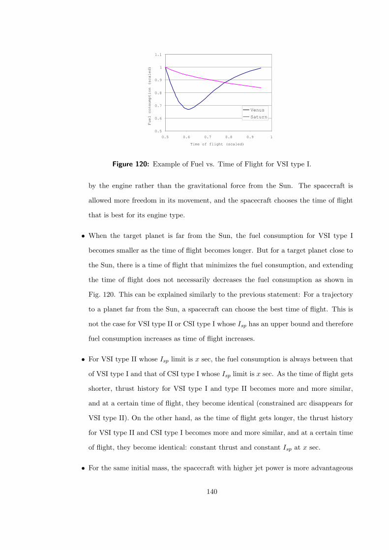
0.5
0.6
0.7
0.8
0.9
1
1.1
0.5 0.6 0.7 0.8 0.9 1
Time of flight (scaled) Fuel consumption (scaled)
Venus
Saturn
Figure 120: Example of Fuel vs. Time of Flight for VSI type I.
by the engine rather than the gravitational force from the Sun. The spacecraft is
allowed more freedom in its movement, and the spacecraft chooses the time of flight
that is best for its engine type.
• When the target planet is far from the Sun, the fuel consumption for VSI type I
becomes smaller as the time of flight becomes longer. But for a target planet close to
the Sun, there is a time of flight that minimizes the fuel consumption, and extending
the time of flight does not necessarily decreases the fuel consumption as shown in
Fig. 120. This can be explained similarly to the previous statement: For a trajectory
to a planet far from the Sun, a spacecraft can choose the best time of flight. This is
not the case for VSI type II or CSI type I whose Isp has an upper bound and therefore
fuel consumption increases as time of flight increases.
• For VSI type II whose Isp limit is x sec, the fuel consumption is always between that
of VSI type I and that of CSI type I whose Isp limit is x sec. As the time of flight gets
shorter, thrust history for VSI type I and type II becomes more and more similar,
and at a certain time of flight, they become identical (constrained arc disappears for
VSI type II). On the other hand, as the time of flight gets longer, the thrust history
for VSI type II and CSI type I becomes more and more similar, and at a certain time
of flight, they become identical: constant thrust and constant Isp at x sec.
• For the same initial mass, the spacecraft with higher jet power is more advantageous
140
than lower jet power. That means the merit of using a VSI engine increases as the jet
power increases for a certain mass of spacecraft. This statement can be also rephrased
as the following way: for the same jet power, a lighter spacecraft is more advantageous
than heavier one. Therefore the merit of using a VSI engine increases as the mass of
spacecraft decreases for a certain jet power.
• The merit of using a VSI engine against using a CSI engine may increase or decrease
as the travel distance increases. It depends on how the problem is set:
– If the Isp of the CSI engine is fixed for any mission profile (time of flight and
target conditions), the merit of using a VSI engine increases as the travel distance
increases. Therefore, using a VSI engine for a transfer to Pluto is the most
effective.
– If the best Isp level for the CSI engine is chosen for each mission depending
on the mission profile, the merit of using a VSI engine decreases as the travel
distance increases. Hence, using a VSI engine for a transfer to Mercury is the
most effective.
• Fuel can be saved by applying swing-by maneuvers for VSI engines, CSI type II, and
high thrust. However, effects of swing-by on VSI engines are smaller than that of high
thrust or CSI engines. This is because for VSI engines unnecessary increase of the
specific energy is observed after swing-by maneuvers, and therefore more fuel than
required is consumed. This is an unnecessary increase of the specific energy that is
not observed for high thrust and CSI type II engines.
9.2 Research Accomplishments
In this section, research goals and objectives presented in Chap. 1 are presented.
• The primary goal of this research is to show the advantages and disadvantages of VSI
engines over conventional engines such as CSI engines and high thrust engines that
are currently used for interplanetary missions. As stated in the previous section, it is
concluded that VSI engines are better than CSI engines and high thrust engines.
141
• The objective that supports the primary goal is to establish a generalized rule that
1. qualitatively states the advantages and disadvantages of VSI engines
2. quantitatively determines the fuel savings by using VSI engines over CSI or high
thrust engines.
As stated in the last section, the 1st rule was established as the relationship between
the fuel savings and the jet power, or the relationship between the fuel savings and
the travel distance. Establishing the 2nd rule was difficult. The fuel consumption is
a function of many parameters such as jet power, time of flight, Isp constraints, and
the configuration of the two planets. Numerically, it is even affected by the number of
time steps or the tolerance for the convergence criteria. However, estimating the fuel
savings is not impossible. From the parameters such as jet power and configuration
of the planets, Tables 5 to 6 will help roughly estimate the fuel savings.
• To support the above goals, it was also a goal to create an interplanetary trajectory
optimization program that can calculate the trajectories for VSI, CSI, and high thrust
engines. The software application SAMURAI – Simulation and Animation Model
Used for Rockets with Adjustable Isp – was created. This application can calculate the
trajectory for each of the five propulsion systems. SAMURAI also conducts planetary
swing-bys if desired, and SAMURAI has a capability of drawing an animation of the
resulted trajectory on a web browser using VRML. Although this application was
developed for the purpose of study of this research, it has a potential to be widely
used for any interplanetary mission analyses, and that is the hope of the author.
9.3 Recommended Future Work
Multiple Swing-bys Current SAMURAI has a capability of calculating a swing-by tra-
jectory with only one planet, but not more than one. This limitation might not be desirable
if Mars missions are to be analyzed because previous studies show that some missions to
Mars do multiple swing-bys with Venus and Earth before arriving at Mars.
142
Using SAMURAI and an existing interplanetary calculation application IPREP (Inter-
planetary PREProcessor), several calculations have been performed for high thrust trajecto-
ries with and without swing-bys. This is to investigate if more ∆V is required for a swing-by
trajectory with only one planet than for a trajectory without swing-by. The results showed
that the ∆V for a trajectory with a single swing-by with Venus is worth than the ∆V for
a trajectory without swing-by.
Therefore, adding a feature of multiple swing-by may improve the mission analysis and
give broader knowledge about VSI engines.
Mission to the Moon In this research only trajectories from Earth to other planets
were investigated. Although VSI engines may be the best for the fast transfers between two
planets, studying about the mission to the Moon with VSI engines may give us interesting
results. Some minor modifications of SAMURAI should make SAMURAI suitable for an-
alyzing the Moon missions because the equations of motion are the same for a trajectory
around the Sun and a trajectory around the Earth.
Optimization Methods for Swing-by, Lagrange Multipliers Currently SAMURAI
employs Powell’s method to find the optimal values for parameters such as conditions at
the entry point of the sphere of influence or the Lagrange multipliers for VSI type II and
CSI type II. Powell’s method works well for most of these problems because in many of
the cases the response surface for these parameters should be near-quadratic. However,
some problems require long computational time or they do not converge. Exploring other
methods such as sequential quadratic programming and applying it to SAMURAI may
improve the robustness and computation time.
143
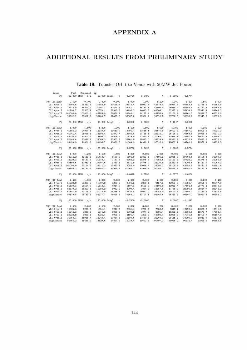
APPENDIX A
ADDITIONAL RESULTS FROM PRELIMINARY STUDY
Table 19: Transfer Orbit to Venus with 20MW Jet Power.
Venus Fuel Consumed (kg)
Pj 20.000 (MW) nju 60.000 (deg) r 0.3750 0.6495 V -1.0000 0.5774
TOF (TU_Sun) 0.600 0.700 0.800 0.900 1.000 1.100 1.200 1.300 1.400 1.500 1.600
VSI type I 75460.6 55333.1 37883.9 31468.9 33372.4 38092.8 42879.0 46934.2 50183.6 52746.8 54765.5
VSI typeII 75472.9 55374.2 37907.7 31497.4 33441.1 38137.8 42896.0 46939.7 50185.4 52747.3 54765.5
CSI type I 91998.7 70503.4 47570.1 37915.3 39492.3 44013.7 48504.1 52327.1 55439.9 57940.4 59943.2
CSI typeII 100000.0 100000.0 42789.9 36856.1 38444.1 44127.1 48138.6 52150.2 56161.7 58919.7 65522.0
highThrust 99962.2 99517.3 98209.7 97435.0 98007.0 98951.2 99520.5 99780.0 99893.8 99945.5 99970.3
Pj 20.000 (MW) nju 90.000 (deg) r -0.0000 0.7500 V -1.1547 -0.0000
TOF (TU_Sun) 1.000 1.100 1.200 1.300 1.400 1.500 1.600 1.700 1.800 1.900 2.000
VSI type I 41684.2 24944.3 14710.8 11680.0 13491.7 17538.3 22175.9 26622.2 30587.2 34009.2 36921.2
VSI typeII 41741.4 25096.1 14888.4 11872.7 13746.5 17768.4 22332.1 26728.1 30663.5 34068.8 36971.2
CSI type I 55130.8 34204.4 19806.3 15209.7 17879.9 22580.4 27468.1 31995.3 35991.9 39441.8 42392.2
CSI typeII 50144.4 33095.3 24069.3 23902.2 32761.0 28833.0 33429.6 38360.5 43625.6 47637.2 48472.9
highThrust 99199.9 96601.8 92196.7 90080.6 91669.9 94920.9 97316.9 98602.2 99248.9 99578.9 99753.5
Pj 20.000 (MW) nju 120.000 (deg) r -0.3750 0.6495 V -1.0000 -0.5774
TOF (TU_Sun) 1.000 1.200 1.400 1.600 1.800 2.000 2.200 2.400 2.600 2.800 3.000
VSI type I 74914.2 49139.3 21413.7 6560.0 5604.9 10843.1 17186.2 22845.2 27463.5 31126.4 34009.9
VSI typeII 74929.3 49187.9 21618.1 7137.3 6362.2 11376.8 17558.6 23143.6 27728.2 31376.8 34256.9
CSI type I 89850.6 62939.8 29707.6 9353.5 8174.9 14876.2 22025.9 28210.4 33208.6 37160.9 40269.3
CSI typeII 100000.0 57164.6 38611.2 17383.4 18052.0 30086.7 33095.3 38109.8 43458.5 49141.5 52651.6
highThrust 99995.2 99784.6 96844.2 83979.1 81463.7 91996.8 97086.1 98835.5 99480.0 99743.9 99863.0
Pj 20.000 (MW) nju 150.000 (deg) r -0.6495 0.3750 V -0.5773 -1.0000
TOF (TU_Sun) 1.400 1.600 1.800 2.000 2.200 2.400 2.600 2.800 3.000 3.200 3.400
VSI type I 51039.2 28338.6 11307.8 3388.9 2504.3 5208.1 9157.3 13203.8 16893.4 20096.8 22817.9
VSI typeII 51139.3 28554.0 11813.1 4814.9 5107.3 6593.9 10100.9 13989.7 17604.6 20771.4 23476.3
CSI type I 64679.2 38200.1 16350.2 5082.5 3909.4 7884.5 12857.8 17738.0 22090.5 25814.7 28944.2
CSI typeII 60841.9 40115.5 27078.0 18386.3 12870.4 18052.0 28248.0 30420.9 37608.3 42789.9 42622.8
highThrust 99879.8 98789.1 92977.7 76848.6 70563.1 83707.4 92446.6 96349.1 98107.2 98950.3 99382.1
Pj 20.000 (MW) nju 180.000 (deg) r -0.7500 -0.0000 V 0.0000 -1.1547
TOF (TU_Sun) 2.000 2.200 2.400 2.600 2.800 3.000 3.200 3.400 3.600 3.800 4.000
VSI type I 15564.6 6200.8 1951.1 1240.3 2531.4 4761.0 7308.9 9849.4 12229.4 14388.2 16311.5
VSI typeII 16044.3 7236.2 5571.6 6035.9 6500.2 7074.6 8995.4 11302.9 13569.5 15670.7 17568.1
CSI type I 22038.8 9288.4 3034.1 1995.6 4191.4 7303.0 10692.1 13986.5 17016.5 19723.7 22107.0
CSI typeII 31758.1 45965.7 14040.4 10864.6 16380.5 17550.5 24069.3 28415.2 33095.3 34933.9 40115.5
highThrust 96465.2 88436.0 73129.6 64867.6 75219.4 85622.9 91707.3 95046.0 96914.4 97999.5 98654.8
144
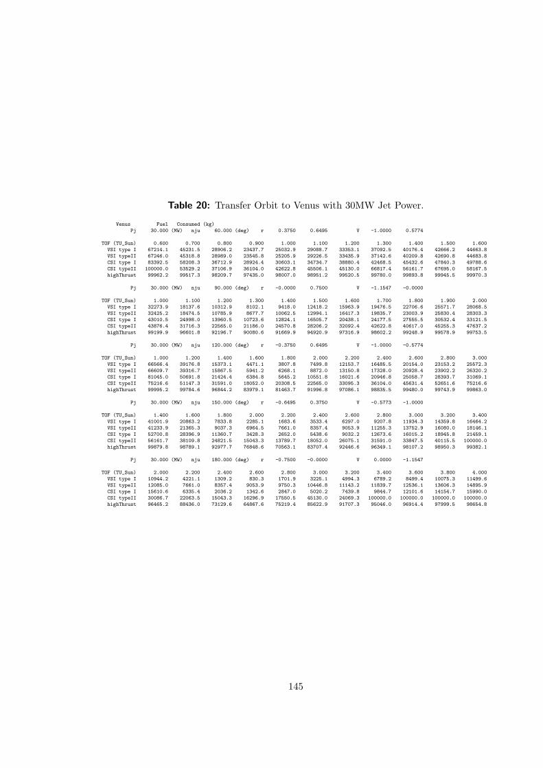
Table 20: Transfer Orbit to Venus with 30MW Jet Power.
Venus Fuel Consumed (kg)
Pj 30.000 (MW) nju 60.000 (deg) r 0.3750 0.6495 V -1.0000 0.5774
TOF (TU_Sun) 0.600 0.700 0.800 0.900 1.000 1.100 1.200 1.300 1.400 1.500 1.600
VSI type I 67214.1 45231.5 28906.2 23437.7 25032.9 29088.7 33353.1 37092.5 40176.4 42666.2 44663.8
VSI typeII 67246.0 45318.8 28989.0 23545.8 25205.9 29226.5 33435.9 37142.6 40209.8 42690.8 44683.8
CSI type I 83392.5 58208.3 36712.9 28924.4 30603.1 34734.7 38880.4 42468.5 45432.6 47840.3 49788.6
CSI typeII 100000.0 53529.2 37106.9 36104.0 42622.8 45506.1 45130.0 66817.4 56161.7 67695.0 58167.5
highThrust 99962.2 99517.3 98209.7 97435.0 98007.0 98951.2 99520.5 99780.0 99893.8 99945.5 99970.3
Pj 30.000 (MW) nju 90.000 (deg) r -0.0000 0.7500 V -1.1547 -0.0000
TOF (TU_Sun) 1.000 1.100 1.200 1.300 1.400 1.500 1.600 1.700 1.800 1.900 2.000
VSI type I 32273.9 18137.6 10312.9 8102.1 9418.0 12418.2 15963.9 19476.5 22706.6 25571.7 28068.5
VSI typeII 32425.2 18474.5 10785.9 8677.7 10062.5 12994.1 16417.3 19835.7 23003.9 25830.4 28303.3
CSI type I 43010.5 24998.0 13960.5 10723.6 12824.1 16505.7 20438.1 24177.5 27555.5 30532.4 33121.5
CSI typeII 43876.4 31716.3 22565.0 21186.0 24570.8 28206.2 32092.4 42622.8 40617.0 45255.3 47637.2
highThrust 99199.9 96601.8 92196.7 90080.6 91669.9 94920.9 97316.9 98602.2 99248.9 99578.9 99753.5
Pj 30.000 (MW) nju 120.000 (deg) r -0.3750 0.6495 V -1.0000 -0.5774
TOF (TU_Sun) 1.000 1.200 1.400 1.600 1.800 2.000 2.200 2.400 2.600 2.800 3.000
VSI type I 66566.4 39176.8 15373.1 4471.1 3807.8 7499.8 12153.7 16485.5 20154.0 23153.2 25572.3
VSI typeII 66609.7 39316.7 15867.5 5941.2 6268.1 8872.0 13150.8 17328.0 20928.4 23902.2 26320.2
CSI type I 81045.0 50691.8 21424.4 6384.8 5645.2 10551.8 16021.6 20946.8 25058.7 28393.7 31069.1
CSI typeII 75216.6 51147.3 31591.0 18052.0 20308.5 22565.0 33095.3 36104.0 45631.4 52651.6 75216.6
highThrust 99995.2 99784.6 96844.2 83979.1 81463.7 91996.8 97086.1 98835.5 99480.0 99743.9 99863.0
Pj 30.000 (MW) nju 150.000 (deg) r -0.6495 0.3750 V -0.5773 -1.0000
TOF (TU_Sun) 1.400 1.600 1.800 2.000 2.200 2.400 2.600 2.800 3.000 3.200 3.400
VSI type I 41001.9 20863.2 7833.8 2285.1 1683.6 3533.4 6297.0 9207.8 11934.3 14359.8 16464.2
VSI typeII 41233.9 21365.3 9037.3 6964.5 7661.0 8357.4 9053.9 11255.3 13752.9 16080.0 18146.1
CSI type I 52700.8 28396.9 11360.7 3428.3 2652.0 5438.6 9032.2 12673.6 16015.2 18945.8 21459.1
CSI typeII 56161.7 38109.8 24821.5 15043.3 13789.7 18052.0 26075.1 31591.0 33847.5 40115.5 100000.0
highThrust 99879.8 98789.1 92977.7 76848.6 70563.1 83707.4 92446.6 96349.1 98107.2 98950.3 99382.1
Pj 30.000 (MW) nju 180.000 (deg) r -0.7500 -0.0000 V 0.0000 -1.1547
TOF (TU_Sun) 2.000 2.200 2.400 2.600 2.800 3.000 3.200 3.400 3.600 3.800 4.000
VSI type I 10944.2 4221.1 1309.2 830.3 1701.9 3225.1 4994.3 6789.2 8499.4 10075.3 11499.6
VSI typeII 12085.0 7661.0 8357.4 9053.9 9750.3 10446.8 11143.2 11839.7 12536.1 13606.3 14895.9
CSI type I 15610.6 6335.4 2036.2 1342.6 2847.0 5020.2 7439.8 9844.7 12101.6 14154.7 15990.0
CSI typeII 30086.7 22063.5 15043.3 16296.9 17550.5 45130.0 24069.3 100000.0 100000.0 100000.0 100000.0
highThrust 96465.2 88436.0 73129.6 64867.6 75219.4 85622.9 91707.3 95046.0 96914.4 97999.5 98654.8
145

Table 21: Transfer Orbit to Mars with 10MW Jet Power.
Mars Fuel Consumed (kg)
Pj 10.000 (MW) nju 60.000 (deg) r 0.7500 1.2990 V -0.7071 0.4082
TOF (TU_Sun) 1.000 1.200 1.400 1.600 1.800 2.000 2.200 2.400 2.600 2.800 3.000
VSI type I 79408.5 61606.1 47004.4 41423.9 41965.7 44635.0 47528.4 50048.1 52091.7 53705.2 54964.0
VSI typeII 79414.2 61614.3 47009.5 41449.5 42047.2 44712.1 47576.1 50077.0 52110.4 53718.3 54974.0
CSI type I 87181.9 69845.2 57111.4 54419.3 57128.6 60687.3 63716.2 66008.5 67660.3 68807.4 69570.4
CSI typeII 100000.0 100000.0 100000.0 48807.2 50395.1 53487.4 56997.5 59170.4 67360.7 65522.0 66441.4
highThrust 99967.2 99643.5 98934.1 98558.6 98794.2 99254.3 99593.6 99781.4 99878.4 99929.2 99956.7
Pj 10.000 (MW) nju 90.000 (deg) r -0.0000 1.5000 V -0.8165 -0.0000
TOF (TU_Sun) 1.600 1.800 2.000 2.200 2.400 2.600 2.800 3.000 3.200 3.400 3.600
VSI type I 52612.7 34420.2 22335.6 17921.9 18736.4 21928.2 25761.6 29449.8 32714.5 35503.2 37846.4
VSI typeII 52627.3 34477.5 22396.5 18006.8 18911.1 22160.7 25959.4 29604.2 32838.6 35607.1 37938.0
CSI type I 58608.9 40521.7 27802.8 24128.0 27162.8 32041.5 36853.9 41065.3 44567.3 47414.9 49702.4
CSI typeII 56161.7 39112.6 29250.9 26660.1 28080.9 31507.4 36271.1 41369.1 44127.1 48305.8 51147.3
highThrust 99544.1 97903.7 95112.7 93454.1 93878.0 95641.3 97361.7 98473.3 99104.8 99457.6 99658.9
Pj 10.000 (MW) nju 120.000 (deg) r -0.7500 1.2990 V -0.7071 -0.4082
TOF (TU_Sun) 2.000 2.200 2.400 2.600 2.800 3.000 3.200 3.400 3.600 3.800 4.000
VSI type I 49261.4 33360.6 20285.3 11933.7 8234.4 7930.3 9621.9 12265.4 15221.2 18145.8 20874.8
VSI typeII 49278.2 33415.1 20430.7 12185.9 8578.9 8375.6 10127.5 12759.9 15662.1 18538.1 21230.8
CSI type I 55204.5 39177.4 25461.6 15715.4 11051.3 11872.3 15087.1 18902.7 22736.7 26321.4 29540.5
CSI typeII 53487.4 38611.2 29083.8 26075.1 18720.6 18804.2 20057.8 26994.4 27078.0 31758.1 35101.1
highThrust 99644.3 98507.0 95434.2 90129.7 85574.1 84744.6 87331.3 91130.8 94232.7 96288.8 97575.1
Pj 10.000 (MW) nju 150.000 (deg) r -1.2990 0.7500 V -0.4082 -0.7071
TOF (TU_Sun) 3.000 3.200 3.400 3.600 3.800 4.000 4.200 4.400 4.600 4.800 5.000
VSI type I 12905.5 7430.8 4572.3 3700.7 4175.4 5473.8 7219.5 9162.5 11147.5 13081.4 14914.5
VSI typeII 13203.7 7934.8 5356.1 4753.6 5397.9 6588.9 8188.1 10019.7 11933.4 13818.8 15617.8
CSI type I 17181.4 10394.2 6346.7 5428.2 6904.0 9151.1 11765.3 14462.9 16993.3 19474.7 21775.7
CSI typeII 26325.8 20057.8 14207.6 15043.3 14291.2 16714.8 21060.7 22063.5 26910.8 30086.7 33429.6
highThrust 93009.0 86705.5 79495.9 75314.1 76448.8 81046.5 86048.4 90035.3 92892.5 94876.2 96249.8
Pj 10.000 (MW) nju 180.000 (deg) r -1.5000 -0.0000 V 0.0000 -0.8165
TOF (TU_Sun) 3.000 3.200 3.400 3.600 3.800 4.000 4.200 4.400 4.600 4.800 5.000
VSI type I 29615.1 20793.0 13728.2 8527.5 5049.8 3014.4 2100.0 2005.5 2480.1 3328.2 4405.8
VSI typeII 29768.1 21023.1 14075.4 9059.4 5913.8 4643.0 4875.2 5107.3 5339.5 5659.8 7784.6
CSI type I 36181.1 26430.4 18252.6 11895.2 7352.7 4422.1 2962.3 3385.1 6057.8 9658.5 9158.2
CSI typeII 38861.9 36104.0 29835.9 24069.3 17467.0 15043.3 12285.4 12870.4 13455.4 22063.5 16714.8
highThrust 98824.9 97418.4 94892.9 90837.7 85117.1 78401.6 72711.3 70651.6 72753.6 77052.0 81602.4
146
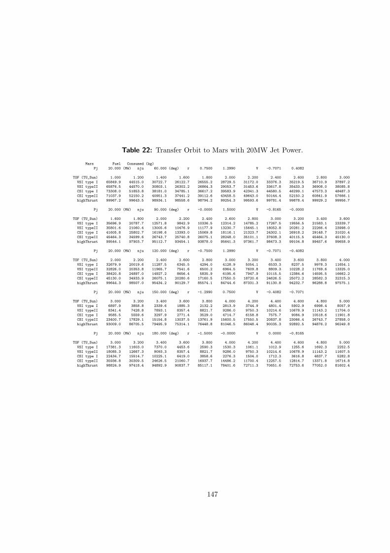
Table 22: Transfer Orbit to Mars with 20MW Jet Power.
Mars Fuel Consumed (kg)
Pj 20.000 (MW) nju 60.000 (deg) r 0.7500 1.2990 V -0.7071 0.4082
TOF (TU_Sun) 1.000 1.200 1.400 1.600 1.800 2.000 2.200 2.400 2.600 2.800 3.000
VSI type I 65849.9 44515.0 30722.7 26122.7 26555.2 28729.5 31172.0 33376.3 35219.5 36710.9 37897.2
VSI typeII 65876.5 44570.0 30803.1 26302.2 26864.3 29053.7 31453.6 33617.8 35433.3 36908.0 38085.8
CSI type I 73308.0 51853.8 38181.0 34785.1 36617.2 39583.9 42341.3 44580.5 46299.1 47573.3 48487.3
CSI typeII 71037.9 52150.2 40951.3 37441.2 39112.6 43458.5 49643.0 50144.4 52150.2 60841.9 57666.1
highThrust 99967.2 99643.5 98934.1 98558.6 98794.2 99254.3 99593.6 99781.4 99878.4 99929.2 99956.7
Pj 20.000 (MW) nju 90.000 (deg) r -0.0000 1.5000 V -0.8165 -0.0000
TOF (TU_Sun) 1.600 1.800 2.000 2.200 2.400 2.600 2.800 3.000 3.200 3.400 3.600
VSI type I 35696.9 20787.7 12571.8 9842.9 10336.5 12314.2 14785.2 17267.5 19556.5 21583.1 23339.7
VSI typeII 35801.6 21060.4 13005.6 10476.9 11177.9 13230.7 15645.1 18052.8 20281.2 22266.4 23998.0
CSI type I 41605.8 25802.7 16198.6 13393.0 15069.8 18116.1 21323.7 24302.1 26918.2 29148.7 31020.4
CSI typeII 45464.3 34599.6 26743.7 25740.8 26075.1 28248.0 35101.1 37608.3 40115.5 45464.3 45130.0
highThrust 99544.1 97903.7 95112.7 93454.1 93878.0 95641.3 97361.7 98473.3 99104.8 99457.6 99658.9
Pj 20.000 (MW) nju 120.000 (deg) r -0.7500 1.2990 V -0.7071 -0.4082
TOF (TU_Sun) 2.000 2.200 2.400 2.600 2.800 3.000 3.200 3.400 3.600 3.800 4.000
VSI type I 32679.9 20019.6 11287.5 6345.5 4294.0 4128.9 5054.1 6533.3 8237.5 9978.3 11654.1
VSI typeII 32826.0 20353.8 11965.7 7541.6 6500.2 6964.5 7609.8 8809.3 10228.2 11769.6 13325.0
CSI type I 38420.8 24897.0 14927.2 8656.4 5835.9 6195.6 7947.9 10115.5 12384.6 14595.5 16662.2
CSI typeII 45130.0 34933.9 26075.1 20280.6 17160.5 17550.5 18720.6 24626.5 25072.2 28582.3 32315.3
highThrust 99644.3 98507.0 95434.2 90129.7 85574.1 84744.6 87331.3 91130.8 94232.7 96288.8 97575.1
Pj 20.000 (MW) nju 150.000 (deg) r -1.2990 0.7500 V -0.4082 -0.7071
TOF (TU_Sun) 3.000 3.200 3.400 3.600 3.800 4.000 4.200 4.400 4.600 4.800 5.000
VSI type I 6897.9 3858.8 2339.6 1885.3 2132.2 2813.9 3744.9 4801.4 5902.9 6998.4 8057.9
VSI typeII 8341.4 7428.8 7893.1 8357.4 8821.7 9286.0 9750.3 10214.6 10678.9 11143.2 11704.0
CSI type I 9585.5 5559.6 3297.9 2771.4 3529.0 4714.7 6158.8 7575.7 9084.9 10518.6 11901.8
CSI typeII 23400.7 17829.1 15154.8 13037.5 13761.9 15600.5 17550.5 20837.8 23066.4 26743.7 27858.0
highThrust 93009.0 86705.5 79495.9 75314.1 76448.8 81046.5 86048.4 90035.3 92892.5 94876.2 96249.8
Pj 20.000 (MW) nju 180.000 (deg) r -1.5000 -0.0000 V 0.0000 -0.8165
TOF (TU_Sun) 3.000 3.200 3.400 3.600 3.800 4.000 4.200 4.400 4.600 4.800 5.000
VSI type I 17381.3 11603.0 7370.0 4453.6 2590.3 1530.3 1061.1 1012.9 1255.6 1692.3 2252.5
VSI typeII 18085.3 12667.3 9093.3 8357.4 8821.7 9286.0 9750.3 10214.6 10678.9 11143.2 11607.5
CSI type I 22434.7 15514.7 10225.1 6419.0 3858.6 2276.3 1504.0 1712.3 3616.8 4837.7 5282.8
CSI typeII 35936.8 30309.5 24626.5 21060.7 16937.7 14486.2 11700.4 12257.5 12814.7 13371.8 16714.8
highThrust 98824.9 97418.4 94892.9 90837.7 85117.1 78401.6 72711.3 70651.6 72753.6 77052.0 81602.4
147
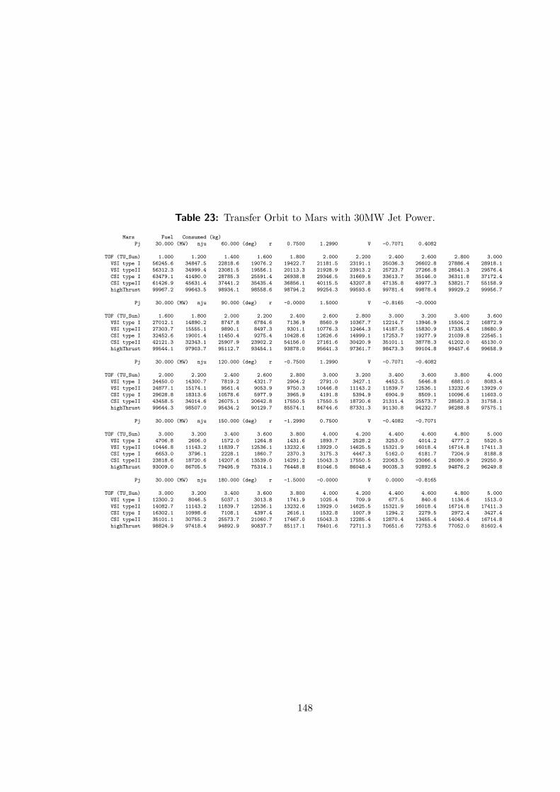
Table 23: Transfer Orbit to Mars with 30MW Jet Power.
Mars Fuel Consumed (kg)
Pj 30.000 (MW) nju 60.000 (deg) r 0.7500 1.2990 V -0.7071 0.4082
TOF (TU_Sun) 1.000 1.200 1.400 1.600 1.800 2.000 2.200 2.400 2.600 2.800 3.000
VSI type I 56245.6 34847.5 22818.6 19076.2 19422.7 21181.5 23191.1 25036.3 26602.8 27886.4 28918.1
VSI typeII 56312.3 34999.4 23081.5 19556.1 20113.3 21928.9 23913.2 25723.7 27266.8 28541.3 29576.4
CSI type I 63479.1 41490.0 28785.3 25591.4 26938.8 29346.5 31669.5 33613.7 35146.0 36311.8 37172.4
CSI typeII 61426.9 45631.4 37441.2 35435.4 36856.1 40115.5 43207.8 47135.8 49977.3 53821.7 55158.9
highThrust 99967.2 99643.5 98934.1 98558.6 98794.2 99254.3 99593.6 99781.4 99878.4 99929.2 99956.7
Pj 30.000 (MW) nju 90.000 (deg) r -0.0000 1.5000 V -0.8165 -0.0000
TOF (TU_Sun) 1.600 1.800 2.000 2.200 2.400 2.600 2.800 3.000 3.200 3.400 3.600
VSI type I 27012.1 14890.2 8747.8 6784.6 7136.9 8560.9 10367.7 12214.7 13946.9 15504.2 16872.9
VSI typeII 27303.7 15555.1 9890.1 8497.3 9301.1 10776.3 12464.3 14187.5 15830.9 17335.4 18680.9
CSI type I 32452.6 19001.4 11450.4 9275.4 10428.6 12626.6 14999.1 17253.7 19277.9 21039.8 22545.1
CSI typeII 42121.3 32343.1 25907.9 23902.2 54156.0 27161.6 30420.9 35101.1 38778.3 41202.0 45130.0
highThrust 99544.1 97903.7 95112.7 93454.1 93878.0 95641.3 97361.7 98473.3 99104.8 99457.6 99658.9
Pj 30.000 (MW) nju 120.000 (deg) r -0.7500 1.2990 V -0.7071 -0.4082
TOF (TU_Sun) 2.000 2.200 2.400 2.600 2.800 3.000 3.200 3.400 3.600 3.800 4.000
VSI type I 24450.0 14300.7 7819.2 4321.7 2904.2 2791.0 3427.1 4452.5 5646.8 6881.0 8083.4
VSI typeII 24877.1 15174.1 9561.4 9053.9 9750.3 10446.8 11143.2 11839.7 12536.1 13232.6 13929.0
CSI type I 29628.8 18313.6 10578.6 5977.9 3965.9 4191.8 5394.9 6904.9 8509.1 10096.6 11603.0
CSI typeII 43458.5 34014.6 26075.1 20642.8 17550.5 17550.5 18720.6 21311.4 25573.7 28582.3 31758.1
highThrust 99644.3 98507.0 95434.2 90129.7 85574.1 84744.6 87331.3 91130.8 94232.7 96288.8 97575.1
Pj 30.000 (MW) nju 150.000 (deg) r -1.2990 0.7500 V -0.4082 -0.7071
TOF (TU_Sun) 3.000 3.200 3.400 3.600 3.800 4.000 4.200 4.400 4.600 4.800 5.000
VSI type I 4706.8 2606.0 1572.0 1264.8 1431.6 1893.7 2528.2 3253.0 4014.2 4777.2 5520.5
VSI typeII 10446.8 11143.2 11839.7 12536.1 13232.6 13929.0 14625.5 15321.9 16018.4 16714.8 17411.3
CSI type I 6653.0 3796.1 2228.1 1860.7 2370.3 3175.3 4447.3 5162.0 6181.7 7204.9 8188.8
CSI typeII 23818.6 18720.6 14207.6 13539.0 14291.2 15043.3 17550.5 22063.5 23066.4 28080.9 29250.9
highThrust 93009.0 86705.5 79495.9 75314.1 76448.8 81046.5 86048.4 90035.3 92892.5 94876.2 96249.8
Pj 30.000 (MW) nju 180.000 (deg) r -1.5000 -0.0000 V 0.0000 -0.8165
TOF (TU_Sun) 3.000 3.200 3.400 3.600 3.800 4.000 4.200 4.400 4.600 4.800 5.000
VSI type I 12300.2 8046.5 5037.1 3013.8 1741.9 1025.4 709.9 677.5 840.6 1134.6 1513.0
VSI typeII 14082.7 11143.2 11839.7 12536.1 13232.6 13929.0 14625.5 15321.9 16018.4 16714.8 17411.3
CSI type I 16302.1 10998.6 7108.1 4397.4 2616.1 1532.8 1007.9 1294.2 2279.5 2972.4 3427.4
CSI typeII 35101.1 30755.2 25573.7 21060.7 17467.0 15043.3 12285.4 12870.4 13455.4 14040.4 16714.8
highThrust 98824.9 97418.4 94892.9 90837.7 85117.1 78401.6 72711.3 70651.6 72753.6 77052.0 81602.4
148
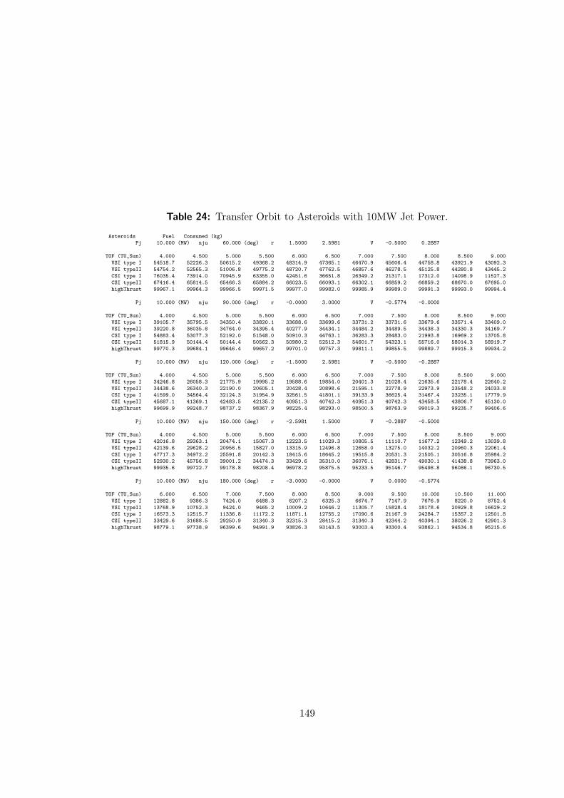
Table 24: Transfer Orbit to Asteroids with 10MW Jet Power.
Asteroids Fuel Consumed (kg)
Pj 10.000 (MW) nju 60.000 (deg) r 1.5000 2.5981 V -0.5000 0.2887
TOF (TU_Sun) 4.000 4.500 5.000 5.500 6.000 6.500 7.000 7.500 8.000 8.500 9.000
VSI type I 54518.7 52226.3 50615.2 49368.2 48314.9 47365.1 46470.9 45606.4 44758.8 43921.9 43092.3
VSI typeII 54754.2 52565.3 51006.8 49775.2 48720.7 47762.5 46857.6 46278.5 45125.8 44280.8 43445.2
CSI type I 76035.4 73914.0 70945.9 63355.0 42451.6 36651.8 26349.2 21317.1 17312.0 14098.9 11527.3
CSI typeII 67416.4 65814.5 65466.3 65884.2 66023.5 66093.1 66302.1 66859.2 66859.2 68670.0 67695.0
highThrust 99967.1 99964.3 99966.5 99971.5 99977.0 99982.0 99985.9 99989.0 99991.3 99993.0 99994.4
Pj 10.000 (MW) nju 90.000 (deg) r -0.0000 3.0000 V -0.5774 -0.0000
TOF (TU_Sun) 4.000 4.500 5.000 5.500 6.000 6.500 7.000 7.500 8.000 8.500 9.000
VSI type I 39105.7 35795.5 34350.4 33820.1 33688.6 33699.6 33731.2 33731.6 33679.6 33571.4 33409.0
VSI typeII 39220.8 36035.8 34764.0 34395.4 40277.9 34434.1 34484.2 34489.5 34438.3 34330.3 34169.7
CSI type I 54883.4 53077.3 52192.0 51548.0 50910.3 44763.1 36283.3 28483.0 21993.8 16969.2 13705.8
CSI typeII 51815.9 50144.4 50144.4 50562.3 50980.2 52512.3 54601.7 54323.1 55716.0 58014.3 58919.7
highThrust 99770.3 99684.1 99646.4 99657.2 99701.0 99757.3 99811.1 99855.5 99889.7 99915.3 99934.2
Pj 10.000 (MW) nju 120.000 (deg) r -1.5000 2.5981 V -0.5000 -0.2887
TOF (TU_Sun) 4.000 4.500 5.000 5.500 6.000 6.500 7.000 7.500 8.000 8.500 9.000
VSI type I 34246.8 26058.3 21775.9 19995.2 19588.6 19854.0 20401.3 21028.4 21635.6 22178.4 22640.2
VSI typeII 34438.6 26340.3 22190.0 20605.1 20428.4 20898.6 21595.1 22778.9 22973.9 23548.2 24033.8
CSI type I 41599.0 34564.4 32124.3 31954.9 32561.5 41801.1 39133.9 36625.4 31467.4 23235.1 17779.9
CSI typeII 45687.1 41369.1 42483.5 42135.2 40951.3 40742.3 40951.3 40742.3 43458.5 43806.7 45130.0
highThrust 99699.9 99248.7 98737.2 98367.9 98225.4 98293.0 98500.5 98763.9 99019.3 99235.7 99406.6
Pj 10.000 (MW) nju 150.000 (deg) r -2.5981 1.5000 V -0.2887 -0.5000
TOF (TU_Sun) 4.000 4.500 5.000 5.500 6.000 6.500 7.000 7.500 8.000 8.500 9.000
VSI type I 42016.8 29363.1 20474.1 15067.3 12223.5 11029.3 10805.5 11110.7 11677.2 12349.2 13039.8
VSI typeII 42139.6 29628.2 20956.5 15827.0 13315.9 12496.8 12658.0 13275.0 14032.2 20960.3 22061.4
CSI type I 47717.3 34972.2 25591.8 20142.3 18415.6 18645.2 19515.8 20531.3 21505.1 30516.8 25984.2
CSI typeII 52930.2 45756.8 39001.2 34474.3 33429.6 35310.0 36076.1 42831.7 49030.1 41438.8 73963.0
highThrust 99935.6 99722.7 99178.8 98208.4 96978.2 95875.5 95233.5 95146.7 95498.8 96086.1 96730.5
Pj 10.000 (MW) nju 180.000 (deg) r -3.0000 -0.0000 V 0.0000 -0.5774
TOF (TU_Sun) 6.000 6.500 7.000 7.500 8.000 8.500 9.000 9.500 10.000 10.500 11.000
VSI type I 12882.8 9386.3 7424.0 6488.3 6207.2 6325.3 6674.7 7147.9 7676.9 8220.0 8752.4
VSI typeII 13768.9 10752.3 9424.0 9465.2 10009.2 10646.2 11305.7 15828.4 18178.6 20929.8 16629.2
CSI type I 16573.3 12515.7 11336.8 11172.2 11871.1 12755.2 17090.6 21167.9 24284.7 15357.2 12501.8
CSI typeII 33429.6 31688.5 29250.9 31340.3 32315.3 28415.2 31340.3 42344.2 40394.1 38026.2 42901.3
highThrust 98779.1 97738.9 96399.6 94991.9 93826.3 93143.5 93003.4 93300.4 93862.1 94534.8 95215.6
149
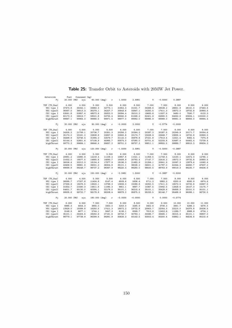
Table 25: Transfer Orbit to Asteroids with 20MW Jet Power.
Asteroids Fuel Consumed (kg)
Pj 20.000 (MW) nju 60.000 (deg) r 1.5000 2.5981 V -0.5000 0.2887
TOF (TU_Sun) 4.000 4.500 5.000 5.500 6.000 6.500 7.000 7.500 8.000 8.500 9.000
VSI type I 37474.8 35342.1 33882.3 32774.1 31852.3 31031.7 30268.6 29539.2 28831.9 28141.0 27463.6
VSI typeII 38357.0 36513.3 35279.1 34327.7 33543.6 32847.1 16250.5 17411.3 18572.0 19732.8 20893.5
CSI type I 53561.8 50857.4 48572.6 35822.5 29394.4 25010.2 19683.8 11927.9 9480.0 7590.7 6122.3
CSI typeII 60173.3 58919.7 58501.8 59755.4 96945.9 61566.2 62401.9 62680.5 64630.6 63934.1 100000.0
highThrust 99967.1 99964.3 99966.5 99971.5 99977.0 99982.0 99985.9 99989.0 99991.3 99993.0 99994.4
Pj 20.000 (MW) nju 90.000 (deg) r -0.0000 3.0000 V -0.5774 -0.0000
TOF (TU_Sun) 4.000 4.500 5.000 5.500 6.000 6.500 7.000 7.500 8.000 8.500 9.000
VSI type I 24305.2 21799.1 20736.7 20351.3 20256.2 20264.2 20287.2 20287.5 20249.9 20171.7 20054.6
VSI typeII 25174.0 23161.2 22608.8 22657.8 22900.8 23174.7 23428.9 23648.7 23835.4 19732.8 20893.5
CSI type I 34499.9 32746.4 31994.2 32579.7 31122.0 30678.8 27221.8 17613.4 12321.4 9382.4 7374.8
CSI typeII 50144.4 52651.6 57108.9 45965.7 83574.0 47080.0 50701.6 52233.8 53487.4 54462.4 72709.4
highThrust 99770.3 99684.1 99646.4 99657.2 99701.0 99757.3 99811.1 99855.5 99889.7 99915.3 99934.2
Pj 20.000 (MW) nju 120.000 (deg) r -1.5000 2.5981 V -0.5000 -0.2887
TOF (TU_Sun) 4.000 4.500 5.000 5.500 6.000 6.500 7.000 7.500 8.000 8.500 9.000
VSI type I 20661.2 14980.9 12218.4 11108.2 10857.6 11021.1 11359.5 11749.5 12130.1 12472.3 12765.1
VSI typeII 21632.0 16577.5 14665.6 14693.7 15408.9 20792.4 17147.7 22416.2 18572.0 19732.8 20893.5
CSI type I 26006.4 20212.3 18154.4 17877.9 18196.3 21482.9 21256.1 20641.9 20067.3 13979.6 10060.4
CSI typeII 43458.5 38861.9 39001.2 38304.8 35101.1 38026.2 39001.2 41787.0 42344.2 44990.7 47637.2
highThrust 99699.9 99248.7 98737.2 98367.9 98225.4 98293.0 98500.5 98763.9 99019.3 99235.7 99406.6
Pj 20.000 (MW) nju 150.000 (deg) r -2.5981 1.5000 V -0.2887 -0.5000
TOF (TU_Sun) 4.000 4.500 5.000 5.500 6.000 6.500 7.000 7.500 8.000 8.500 9.000
VSI type I 26595.7 17207.8 11404.8 8147.4 6509.6 5836.4 5711.2 5882.2 6200.6 6580.9 6974.6
VSI typeII 27258.9 18476.5 13622.1 12768.3 13929.0 15089.8 16250.5 17411.3 18572.5 19732.8 22667.5
CSI type I 31832.7 21580.3 14811.6 11085.3 9851.1 9897.7 10367.5 10945.5 12828.6 18107.3 14175.7
CSI typeII 54601.7 45130.0 40394.1 32176.0 35101.1 36215.4 35101.1 33429.6 35658.3 33151.0 35101.1
highThrust 99935.6 99722.7 99178.8 98208.4 96978.2 95875.5 95233.5 95146.7 95498.8 96086.1 96730.5
Pj 20.000 (MW) nju 180.000 (deg) r -3.0000 -0.0000 V 0.0000 -0.5774
TOF (TU_Sun) 6.000 6.500 7.000 7.500 8.000 8.500 9.000 9.500 10.000 10.500 11.000
VSI type I 6885.3 4924.3 3855.0 3353.0 3203.0 3265.9 3452.6 3706.3 3991.7 4286.2 4576.5
VSI typeII 13929.0 15089.8 16250.5 17411.3 18572.2 19732.8 20903.7 22054.3 23215.0 24375.8 25536.5
CSI type I 9148.9 6677.1 5744.1 5847.3 6138.1 6599.7 7813.8 12453.8 11089.7 9988.9 6734.1
CSI typeII 35101.1 34404.6 29250.9 27161.6 26743.7 30783.1 30086.7 26465.1 36215.4 35101.1 39837.0
highThrust 98779.1 97738.9 96399.6 94991.9 93826.3 93143.5 93003.4 93300.4 93862.1 94534.8 95215.6
150
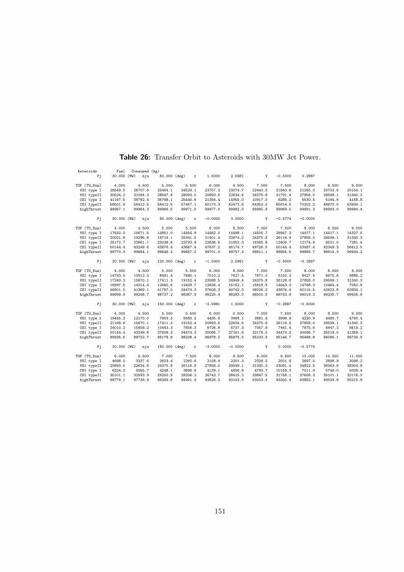
Table 26: Transfer Orbit to Asteroids with 30MW Jet Power.
Asteroids Fuel Consumed (kg)
Pj 30.000 (MW) nju 60.000 (deg) r 1.5000 2.5981 V -0.5000 0.2887
TOF (TU_Sun) 4.000 4.500 5.000 5.500 6.000 6.500 7.000 7.500 8.000 8.500 9.000
VSI type I 28549.5 26707.8 25464.1 24529.1 23757.3 23074.7 22443.5 21843.6 21265.0 20702.6 20154.1
VSI typeII 30524.2 31094.3 28547.8 28093.0 20893.5 22634.6 24375.8 31791.4 27858.0 29599.1 31340.3
CSI type I 41167.5 38762.4 36798.1 25440.6 21356.4 14955.0 10917.0 8285.2 6530.5 5194.9 4168.8
CSI typeII 58501.8 56412.5 56412.5 57457.1 60173.3 62471.6 64352.0 65814.5 70202.2 68670.0 63934.1
highThrust 99967.1 99964.3 99966.5 99971.5 99977.0 99982.0 99985.9 99989.0 99991.3 99993.0 99994.4
Pj 30.000 (MW) nju 90.000 (deg) r -0.0000 3.0000 V -0.5774 -0.0000
TOF (TU_Sun) 4.000 4.500 5.000 5.500 6.000 6.500 7.000 7.500 8.000 8.500 9.000
VSI type I 17632.0 15671.5 14851.0 14554.9 14482.0 14488.1 14505.7 28947.3 14477.1 14417.1 14327.5
VSI typeII 20021.8 19296.6 19719.1 25341.5 21401.4 22674.2 24375.8 26116.9 27858.0 29599.1 31340.3
CSI type I 25172.7 23661.1 23038.6 23793.8 22636.6 21852.3 16365.8 12409.7 12174.9 6531.0 7281.4
CSI typeII 50144.4 43249.6 43876.4 43667.4 47637.2 46174.7 49726.5 50144.4 53487.4 92349.3 56412.5
highThrust 99770.3 99684.1 99646.4 99657.2 99701.0 99757.3 99811.1 99855.5 99889.7 99915.3 99934.2
Pj 30.000 (MW) nju 120.000 (deg) r -1.5000 2.5981 V -0.5000 -0.2887
TOF (TU_Sun) 4.000 4.500 5.000 5.500 6.000 6.500 7.000 7.500 8.000 8.500 9.000
VSI type I 14793.0 10512.2 8491.4 7690.1 7510.2 7627.5 7871.0 8152.3 8427.5 8675.6 8888.2
VSI typeII 17240.3 15670.1 17411.3 19152.4 23588.5 24949.4 24375.8 26126.8 27858.0 29599.1 31340.3
CSI type I 18997.5 14314.4 12660.6 12409.7 12626.4 15152.1 15818.5 14643.3 14768.3 10464.4 7050.9
CSI typeII 46801.5 41369.1 41787.0 34474.3 37608.3 40742.3 38026.2 43876.4 40115.5 42622.8 63934.1
highThrust 99699.9 99248.7 98737.2 98367.9 98225.4 98293.0 98500.5 98763.9 99019.3 99235.7 99406.6
Pj 30.000 (MW) nju 150.000 (deg) r -2.5981 1.5000 V -0.2887 -0.5000
TOF (TU_Sun) 4.000 4.500 5.000 5.500 6.000 6.500 7.000 7.500 8.000 8.500 9.000
VSI type I 19455.2 12170.0 7903.3 5583.2 4435.9 3968.1 3881.4 3999.9 4220.9 4485.7 4760.4
VSI typeII 21168.6 15670.1 17411.3 19152.4 20893.5 22634.6 24375.8 26116.9 27858.0 29599.1 31340.3
CSI type I 24010.2 15658.2 10443.3 7656.3 6726.8 6737.3 7057.8 7461.4 7875.6 8447.2 8619.2
CSI typeII 50144.4 43249.6 37608.3 34474.3 30086.7 27161.6 32176.0 34474.3 30086.7 35519.0 41369.1
highThrust 99935.6 99722.7 99178.8 98208.4 96978.2 95875.5 95233.5 95146.7 95498.8 96086.1 96730.5
Pj 30.000 (MW) nju 180.000 (deg) r -3.0000 -0.0000 V 0.0000 -0.5774
TOF (TU_Sun) 6.000 6.500 7.000 7.500 8.000 8.500 9.000 9.500 10.000 10.500 11.000
VSI type I 4698.0 3337.6 2603.4 2260.6 2158.4 2201.3 2328.5 2501.8 2697.0 2898.9 3098.2
VSI typeII 20893.5 22634.6 24375.8 26116.9 27858.0 29599.1 31340.3 33081.4 34822.5 36563.6 38304.8
CSI type I 6324.2 4555.7 4248.1 3896.6 4139.1 4456.8 4793.7 10159.3 7011.9 5746.0 5028.4
CSI typeII 35101.1 32593.9 29250.9 28206.2 26743.7 28415.2 33847.5 31758.1 37608.3 35101.1 32176.0
highThrust 98779.1 97738.9 96399.6 94991.9 93826.3 93143.5 93003.4 93300.4 93862.1 94534.8 95215.6
151
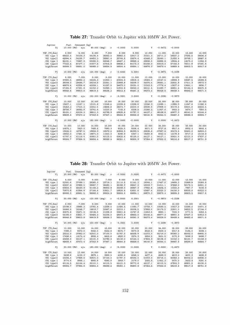
Table 27: Transfer Orbit to Jupiter with 10MW Jet Power.
Jupiter Fuel Consumed (kg)
Pj 10.000 (MW) nju 90.000 (deg) r -0.0000 5.0000 V -0.4472 -0.0000
TOF (TU_Sun) 4.000 5.000 6.000 7.000 8.000 9.000 10.000 11.000 12.000 13.000 14.000
VSI type I 68922.4 54109.3 44194.4 38342.0 34862.0 32617.2 31001.3 29711.2 28597.2 27584.5 26636.6
VSI typeII 68994.4 54235.7 44452.2 38861.4 35744.8 33874.4 42448.3 35060.1 31855.4 29766.1 28967.9
CSI type I 82191.1 70667.9 63066.3 58046.7 49407.1 38829.4 29936.5 24986.9 18634.6 14575.0 11552.9
CSI typeII 77222.4 67277.1 61677.6 57916.8 58836.1 60173.3 61009.0 62513.4 67193.5 79311.8 57331.8
highThrust 99999.3 99991.5 99968.0 99934.9 99904.4 99884.1 99876.3 99879.4 99889.8 99903.5 99917.6
Pj 10.000 (MW) nju 120.000 (deg) r -2.5000 4.3301 V -0.3873 -0.2236
TOF (TU_Sun) 6.000 7.000 8.000 9.000 10.000 11.000 12.000 13.000 14.000 15.000 16.000
VSI type I 37660.5 28892.2 24224.3 21840.1 20604.3 19918.3 19484.3 19157.5 18868.9 18587.5 18299.6
VSI typeII 38009.0 29494.7 25216.5 23351.1 22668.8 34509.0 34375.4 28261.1 22531.8 17411.3 18572.0
CSI type I 48876.4 42256.6 43059.1 41097.5 34475.0 29231.0 21202.5 17776.4 13827.0 13661.1 8826.7
CSI typeII 57164.6 57331.8 52150.2 50395.1 51815.9 49643.0 49141.5 51063.7 46801.5 50144.4 49475.8
highThrust 99946.8 99813.8 99619.5 99436.2 99312.6 99261.3 99273.4 99329.6 99408.4 99492.6 99571.5
Pj 10.000 (MW) nju 150.000 (deg) r -4.3301 2.5000 V -0.2236 -0.3873
TOF (TU_Sun) 10.000 12.000 14.000 16.000 18.000 20.000 22.000 24.000 26.000 28.000 30.000
VSI type I 13407.1 12157.1 12101.6 12246.5 12339.9 12336.6 12246.3 12089.1 11884.3 11647.6 11390.4
VSI typeII 16253.2 17015.2 22551.5 18606.6 28072.7 23215.0 25536.5 27858.0 30179.5 32501.0 34822.5
CSI type I 28756.7 26063.8 15761.6 10220.8 7105.5 6209.5 21280.2 11927.6 5652.2 5674.7 7850.5
CSI typeII 35101.1 43124.2 38611.2 42789.9 43625.6 41787.0 44127.1 48138.6 49977.3 49141.5 50144.4
highThrust 98608.4 97673.4 97543.9 97947.1 98444.9 98849.6 99140.9 99344.5 99487.6 99589.9 99664.7
Pj 10.000 (MW) nju 180.000 (deg) r -5.0000 -0.0000 V 0.0000 -0.4472
TOF (TU_Sun) 10.000 12.000 14.000 16.000 18.000 20.000 22.000 24.000 26.000 28.000 30.000
VSI type I 10675.1 7920.0 7466.6 7680.3 8025.5 8336.4 8571.0 8727.8 8817.4 8852.4 8844.4
VSI typeII 13524.2 16787.5 18806.3 18572.0 20893.5 26293.5 25536.6 27887.6 30179.5 32501.0 34823.0
CSI type I 16642.0 17461.6 18871.0 11500.2 8246.9 6347.1 19293.9 6052.0 13178.8 8717.2 15118.9
CSI typeII 41787.0 41118.4 40951.3 40115.5 43625.6 45130.0 44127.1 44127.1 45631.4 42121.3 47637.2
highThrust 99304.7 97994.9 96654.4 96089.4 96281.1 96800.9 97354.6 97832.8 98216.6 98517.3 98751.9
Table 28: Transfer Orbit to Jupiter with 20MW Jet Power.
Jupiter Fuel Consumed (kg)
Pj 20.000 (MW) nju 90.000 (deg) r -0.0000 5.0000 V -0.4472 -0.0000
TOF (TU_Sun) 4.000 5.000 6.000 7.000 8.000 9.000 10.000 11.000 12.000 13.000 14.000
VSI type I 52581.6 37089.1 28365.3 23718.1 21110.8 31141.2 18344.1 17447.5 16684.2 15998.9 15364.6
VSI typeII 52937.9 37889.5 29967.7 26490.1 36188.2 28647.2 23229.7 31611.1 27858.0 30179.5 32501.0
CSI type I 63502.3 49153.3 41155.2 36602.8 33208.0 26847.3 17842.6 14434.4 10322.3 7957.7 6132.9
CSI typeII 70870.8 61844.8 57164.6 53821.7 54824.6 52651.6 53487.4 53320.2 54156.0 69533.6 65522.0
highThrust 99999.3 99991.5 99968.0 99934.9 99904.4 99884.1 99876.3 99879.4 99889.8 99903.5 99917.6
Pj 20.000 (MW) nju 120.000 (deg) r -2.5000 4.3301 V -0.3873 -0.2236
TOF (TU_Sun) 6.000 7.000 8.000 9.000 10.000 11.000 12.000 13.000 14.000 15.000 16.000
VSI type I 23198.5 16885.2 13781.4 12258.5 11485.4 11060.7 10793.7 10593.5 10417.3 10246.0 10071.3
VSI typeII 24994.9 20248.7 19819.7 20967.6 23215.1 25536.5 27858.0 30179.5 32501.0 34822.5 37144.0
CSI type I 30675.8 24971.0 23126.5 21236.8 25901.9 15797.8 11853.5 9884.1 7322.0 5771.5 5353.4
CSI typeII 54156.0 53821.7 45464.3 54156.0 48472.9 49643.0 50144.4 49977.3 46801.5 47637.2 50813.0
highThrust 99946.8 99813.8 99619.5 99436.2 99312.6 99261.3 99273.4 99329.6 99408.4 99492.6 99571.5
Pj 20.000 (MW) nju 150.000 (deg) r -4.3301 2.5000 V -0.2236 -0.3873
TOF (TU_Sun) 10.000 12.000 14.000 16.000 18.000 20.000 22.000 24.000 26.000 28.000 30.000
VSI type I 7098.0 6472.0 6440.5 6522.6 6575.7 6573.9 6522.5 6433.4 6317.6 6184.0 6039.1
VSI typeII 23215.0 27862.0 32501.0 37144.0 41787.0 46458.9 51073.0 55716.0 60360.2 65002.0 69645.0
CSI type I 17436.4 13174.4 9938.4 5600.6 4820.0 3374.2 5554.5 3521.5 5170.9 3058.3 6698.7
CSI typeII 43458.5 44127.1 42121.3 42789.9 45130.0 50144.4 47804.3 48138.6 52150.2 56161.7 55158.9
highThrust 98608.4 97673.4 97543.9 97947.1 98444.9 98849.6 99140.9 99344.5 99487.6 99589.9 99664.7
Pj 20.000 (MW) nju 180.000 (deg) r -5.0000 -0.0000 V 0.0000 -0.4472
TOF (TU_Sun) 10.000 12.000 14.000 16.000 18.000 20.000 22.000 24.000 26.000 28.000 30.000
VSI type I 5638.6 4123.3 3878.1 3993.5 4180.5 4349.5 4477.4 4563.0 4612.0 4631.2 4626.8
VSI typeII 23239.4 27858.0 32501.0 37144.0 41787.0 46430.0 51073.0 55716.0 60359.0 65002.0 69645.0
CSI type I 8774.6 8848.1 8885.8 6560.6 3849.7 3178.0 2092.9 11401.3 5475.0 3433.9 8291.4
CSI typeII 40115.5 50144.4 35101.1 40115.5 42121.3 36772.6 44127.1 40115.5 47804.3 46801.5 45130.0
highThrust 99304.7 97994.9 96654.4 96089.4 96281.1 96800.9 97354.6 97832.8 98216.6 98517.3 98751.9
152
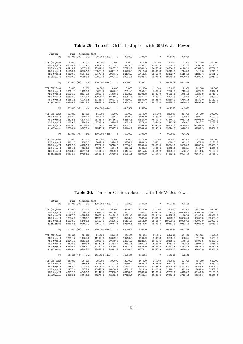
Table 29: Transfer Orbit to Jupiter with 30MW Jet Power.
Jupiter Fuel Consumed (kg)
Pj 30.000 (MW) nju 90.000 (deg) r -0.0000 5.0000 V -0.4472 -0.0000
TOF (TU_Sun) 4.000 5.000 6.000 7.000 8.000 9.000 10.000 11.000 12.000 13.000 14.000
VSI type I 42504.2 28214.2 20884.8 17169.5 15139.3 13893.7 13025.9 12350.0 11777.9 11266.8 10796.0
VSI typeII 43413.9 30371.8 25314.0 25137.0 27892.8 31340.3 34853.6 38304.8 41787.0 45269.3 48751.5
CSI type I 51958.1 37767.8 30533.8 26691.7 24249.9 17712.6 12499.8 10019.3 7146.5 5419.6 4245.6
CSI typeII 69199.3 60173.3 60173.3 59671.9 54156.0 56412.5 55158.9 63432.7 54156.0 61928.4 59671.9
highThrust 99999.3 99991.5 99968.0 99934.9 99904.4 99884.1 99876.3 99879.4 99889.8 99903.5 99917.6
Pj 30.000 (MW) nju 120.000 (deg) r -2.5000 4.3301 V -0.3873 -0.2236
TOF (TU_Sun) 6.000 7.000 8.000 9.000 10.000 11.000 12.000 13.000 14.000 15.000 16.000
VSI type I 16761.8 11928.5 9630.0 8520.5 7961.8 7656.1 7464.4 7320.8 7194.7 7072.2 6947.4
VSI typeII 21596.9 24375.8 27858.0 31340.3 34822.5 38304.8 41787.0 45269.3 48751.5 52233.8 55716.0
CSI type I 22437.8 17741.4 15924.6 16518.3 14814.4 11065.7 8743.5 6794.0 5039.1 3848.4 3207.5
CSI typeII 52651.6 49141.5 54156.0 49643.0 45130.0 46885.0 48138.6 52150.2 49141.5 45130.0 52150.2
highThrust 99946.8 99813.8 99619.5 99436.2 99312.6 99261.3 99273.4 99329.6 99408.4 99492.6 99571.5
Pj 30.000 (MW) nju 150.000 (deg) r -4.3301 2.5000 V -0.2236 -0.3873
TOF (TU_Sun) 10.000 12.000 14.000 16.000 18.000 20.000 22.000 24.000 26.000 28.000 30.000
VSI type I 4907.7 4409.8 4387.8 4445.0 4482.0 4480.8 4445.0 4382.9 4302.3 4209.4 4108.8
VSI typeII 34822.5 41787.0 48751.5 55716.0 62683.3 69645.0 76609.5 83574.0 90538.5 97503.0 100000.0
CSI type I 10639.5 9546.6 5718.2 3599.7 2652.7 3372.8 2044.2 2413.2 3540.2 3420.7 5788.7
CSI typeII 40115.5 45130.0 35101.1 48138.6 40617.0 50144.4 49643.0 54156.0 52150.2 49141.5 60173.3
highThrust 98608.4 97673.4 97543.9 97947.1 98444.9 98849.6 99140.9 99344.5 99487.6 99589.9 99664.7
Pj 30.000 (MW) nju 180.000 (deg) r -5.0000 -0.0000 V 0.0000 -0.4472
TOF (TU_Sun) 10.000 12.000 14.000 16.000 18.000 20.000 22.000 24.000 26.000 28.000 30.000
VSI type I 3831.0 2787.2 2619.2 2698.3 2826.4 2942.3 3030.1 3089.0 3122.7 474.5 3132.8
VSI typeII 34822.5 41787.0 48751.5 55716.0 62680.5 69645.0 76609.5 83574.0 90538.5 97503.0 100000.0
CSI type I 5931.2 6264.0 6552.7 4354.4 2711.1 2168.6 1695.4 3563.3 6223.1 3101.7 2383.5
CSI typeII 37608.3 39112.6 35101.1 32092.4 36104.0 40115.5 38611.2 48138.6 45631.4 49141.5 45130.0
highThrust 99304.7 97994.9 96654.4 96089.4 96281.1 96800.9 97354.6 97832.8 98216.6 98517.3 98751.9
Table 30: Transfer Orbit to Saturn with 10MW Jet Power.
Saturn Fuel Consumed (kg)
Pj 10.000 (MW) nju 120.000 (deg) r -5.0000 8.6603 V -0.2739 -0.1581
TOF (TU_Sun) 20.000 22.000 24.000 26.000 28.000 30.000 32.000 34.000 36.000 38.000 40.000
VSI type I 17892.9 16648.4 15629.8 14756.3 13982.6 13282.7 12640.5 12045.9 100000.0 100000.0 100000.0
VSI typeII 31027.5 25536.5 27858.0 30179.5 32501.0 34822.5 37144.0 39465.5 41787.0 44108.5 100000.0
CSI type I 17555.4 16238.1 11293.8 9867.6 8706.0 7882.0 11860.0 8928.3 100000.0 100000.0 100000.0
CSI typeII 56830.3 51481.6 52150.2 56496.0 56161.7 55158.9 56161.7 100000.0 100000.0 100000.0 100000.0
highThrust 99698.5 99640.2 99600.0 99577.6 99570.8 99576.6 99591.8 99613.1 99637.9 99664.0 99689.9
Pj 10.000 (MW) nju 150.000 (deg) r -8.6603 5.0000 V -0.1581 -0.2739
TOF (TU_Sun) 20.000 22.000 24.000 26.000 28.000 30.000 32.000 34.000 36.000 38.000 40.000
VSI type I 12681.2 11765.2 11117.8 10622.6 10216.5 9864.9 9548.3 9255.6 8980.4 8718.8 8468.7
VSI typeII 28541.7 25536.5 27858.0 30179.5 32501.0 34822.5 40193.6 39465.5 41787.0 44108.5 46430.0
CSI type I 15820.9 13901.6 13730.3 17862.9 9131.8 11561.2 6443.6 6717.2 18626.9 15607.2 7536.4
CSI typeII 56830.3 45965.7 52150.2 52150.2 53821.7 49643.0 45464.3 51147.3 48138.6 47637.2 56830.3
highThrust 99369.4 99086.7 98824.4 98611.2 98460.4 98373.1 98342.9 98358.7 98408.6 98480.9 98566.1
Pj 10.000 (MW) nju 180.000 (deg) r -10.0000 -0.0000 V 0.0000 -0.3162
TOF (TU_Sun) 24.000 26.000 28.000 30.000 32.000 34.000 36.000 38.000 40.000 42.000 44.000
VSI type I 7941.0 7556.6 7296.5 7107.7 6960.2 6836.2 6725.6 6622.4 6523.2 6426.2 6330.2
VSI typeII 27858.0 30179.9 32501.0 37501.6 37144.0 39465.5 41788.3 44108.5 46430.0 48751.5 52091.9
CSI type I 11227.4 15076.9 10948.9 10200.1 16081.4 6412.9 11603.6 31218.0 6418.6 8654.8 21503.5
CSI typeII 46132.9 43458.5 49141.5 37608.3 48138.6 53988.8 45130.0 47637.2 43458.5 49141.5 55158.9
highThrust 99108.2 98745.0 98372.4 98023.9 97725.5 97493.0 97331.2 97236.4 97199.5 97209.0 97253.4
153
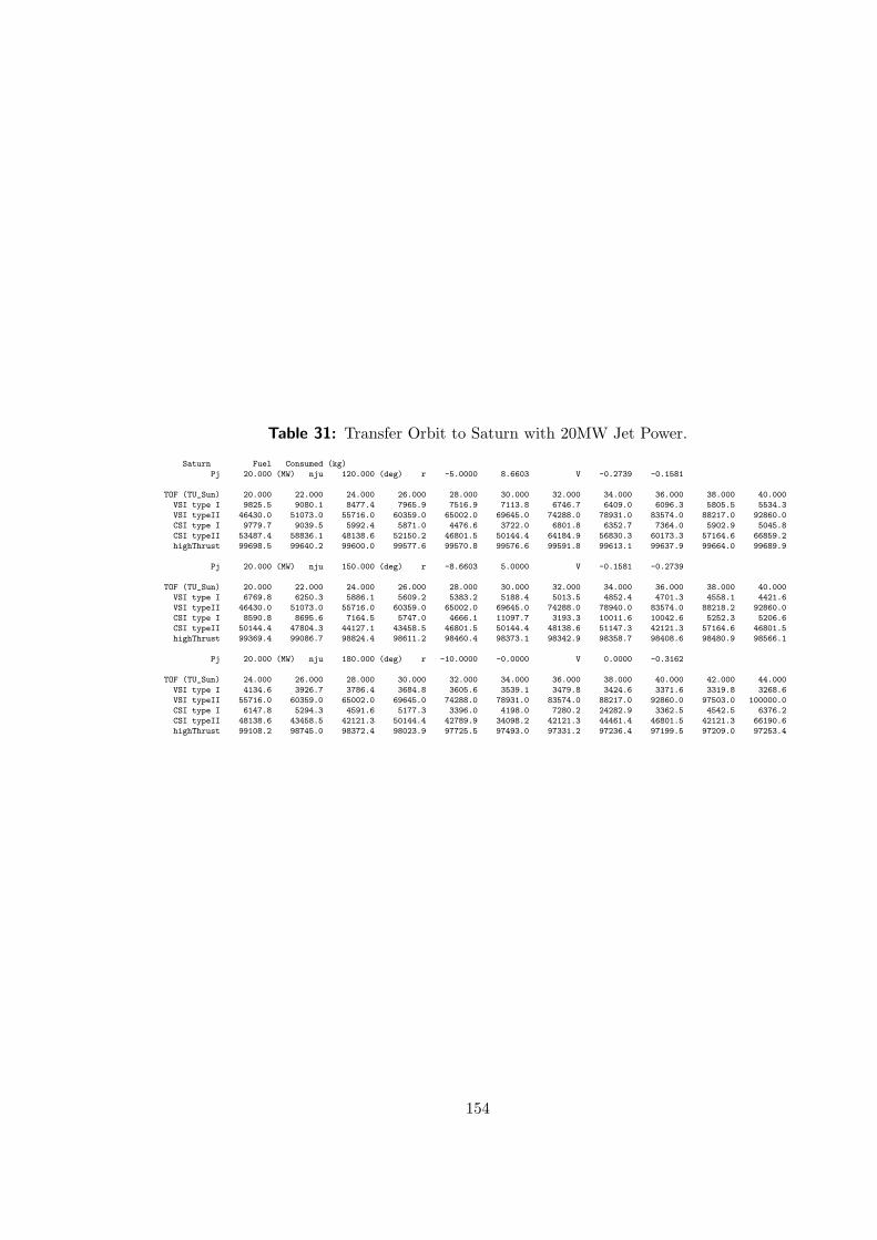
Table 31: Transfer Orbit to Saturn with 20MW Jet Power.
Saturn Fuel Consumed (kg)
Pj 20.000 (MW) nju 120.000 (deg) r -5.0000 8.6603 V -0.2739 -0.1581
TOF (TU_Sun) 20.000 22.000 24.000 26.000 28.000 30.000 32.000 34.000 36.000 38.000 40.000
VSI type I 9825.5 9080.1 8477.4 7965.9 7516.9 7113.8 6746.7 6409.0 6096.3 5805.5 5534.3
VSI typeII 46430.0 51073.0 55716.0 60359.0 65002.0 69645.0 74288.0 78931.0 83574.0 88217.0 92860.0
CSI type I 9779.7 9039.5 5992.4 5871.0 4476.6 3722.0 6801.8 6352.7 7364.0 5902.9 5045.8
CSI typeII 53487.4 58836.1 48138.6 52150.2 46801.5 50144.4 64184.9 56830.3 60173.3 57164.6 66859.2
highThrust 99698.5 99640.2 99600.0 99577.6 99570.8 99576.6 99591.8 99613.1 99637.9 99664.0 99689.9
Pj 20.000 (MW) nju 150.000 (deg) r -8.6603 5.0000 V -0.1581 -0.2739
TOF (TU_Sun) 20.000 22.000 24.000 26.000 28.000 30.000 32.000 34.000 36.000 38.000 40.000
VSI type I 6769.8 6250.3 5886.1 5609.2 5383.2 5188.4 5013.5 4852.4 4701.3 4558.1 4421.6
VSI typeII 46430.0 51073.0 55716.0 60359.0 65002.0 69645.0 74288.0 78940.0 83574.0 88218.2 92860.0
CSI type I 8590.8 8695.6 7164.5 5747.0 4666.1 11097.7 3193.3 10011.6 10042.6 5252.3 5206.6
CSI typeII 50144.4 47804.3 44127.1 43458.5 46801.5 50144.4 48138.6 51147.3 42121.3 57164.6 46801.5
highThrust 99369.4 99086.7 98824.4 98611.2 98460.4 98373.1 98342.9 98358.7 98408.6 98480.9 98566.1
Pj 20.000 (MW) nju 180.000 (deg) r -10.0000 -0.0000 V 0.0000 -0.3162
TOF (TU_Sun) 24.000 26.000 28.000 30.000 32.000 34.000 36.000 38.000 40.000 42.000 44.000
VSI type I 4134.6 3926.7 3786.4 3684.8 3605.6 3539.1 3479.8 3424.6 3371.6 3319.8 3268.6
VSI typeII 55716.0 60359.0 65002.0 69645.0 74288.0 78931.0 83574.0 88217.0 92860.0 97503.0 100000.0
CSI type I 6147.8 5294.3 4591.6 5177.3 3396.0 4198.0 7280.2 24282.9 3362.5 4542.5 6376.2
CSI typeII 48138.6 43458.5 42121.3 50144.4 42789.9 34098.2 42121.3 44461.4 46801.5 42121.3 66190.6
highThrust 99108.2 98745.0 98372.4 98023.9 97725.5 97493.0 97331.2 97236.4 97199.5 97209.0 97253.4
154
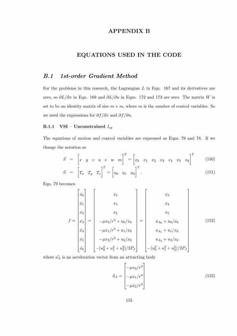
APPENDIX B
EQUATIONS USED IN THE CODE
B.1 1st-order Gradient Method
For the problems in this research, the Lagrangian L in Eqn. 167 and its derivatives are
zero, so ∂L/∂x in Eqn. 169 and ∂L/∂u in Eqns. 172 and 173 are zero. The matrix W is
set to be an identity matrix of size m×m, where m is the number of control variables. So
we need the expressions for ∂f/∂x and ∂f/∂u.
B.1.1 VSI – Unconstrained Isp
The equations of motion and control variables are expressed as Eqns. 79 and 78. If we
change the notation as
~x =
[
x y z u v w m
]T
=
[
x0 x1 x2 x3 x4 x5 x6
]T
(150)
~u =
[
Tx Ty Tz
]T
=
[
u0 u1 u2
]T
, (151)
Eqn. 79 becomes
f =
x0
x1
x2
x3
x4
x5
x6
=
x3
x4
x5
−µx0/r3 + u0/x6
−µx1/r3 + u1/x6
−µx2/r3 + u2/x6
−(u20 + u2
1 + u22)/2PJ
=
x3
x4
x5
aA0+ u0/x6
aA1+ u1/x6
aA2+ u2/x6
−(u20 + u2
1 + u22)/2PJ
(152)
where ~aA is an acceleration vector from an attracting body
~aA =
−µx0/r3
−µx1/r3
−µx2/r3
(153)
155
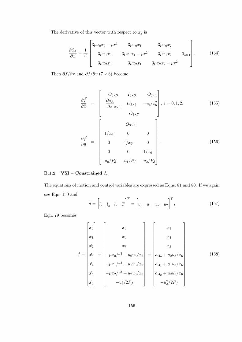
The derivative of this vector with respect to xj is
∂~aA∂~x
=1
r5
3µx0x0 − µr2 3µx0x1 3µx0x2
3µx1x0 3µx1x1 − µr2 3µx1x2 03×4
3µx2x0 3µx2x1 3µx2x2 − µr2
. (154)
Then ∂f/∂x and ∂f/∂u (7 × 3) become
∂ ~f
∂~x=
O3×3 I3×3 O3×1
∂aA∂x 3×3
O3×3 −ui/x26
O1×7
, i = 0, 1, 2. (155)
∂ ~f
∂~u=
O3×3
1/x6 0 0
0 1/x6 0
0 0 1/x6
−u0/PJ −u1/PJ −u2/PJ
. (156)
B.1.2 VSI – Constrained Isp
The equations of motion and control variables are expressed as Eqns. 81 and 80. If we again
use Eqn. 150 and
~u =
[
lx ly lz T
]T
=
[
u0 u1 u2 u2
]T
, (157)
Eqn. 79 becomes
f =
x0
x1
x2
x3
x4
x5
x6
=
x3
x4
x5
−µx0/r3 + u0u3/x6
−µx1/r3 + u1u3/x6
−µx2/r3 + u2u3/x6
−u23/2PJ
=
x3
x4
x5
aA0+ u0u3/x6
aA1+ u1u3/x6
aA2+ u2u3/x6
−u23/2PJ
(158)
156
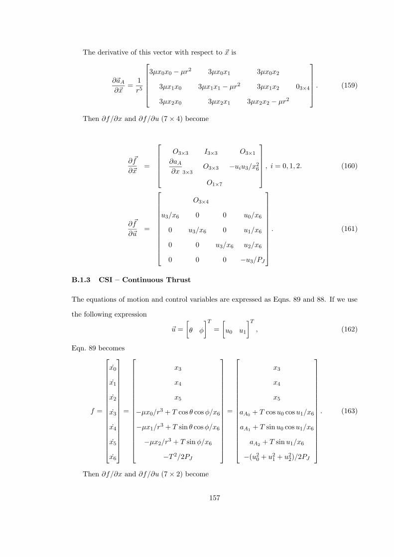
The derivative of this vector with respect to ~x is
∂~aA∂~x
=1
r5
3µx0x0 − µr2 3µx0x1 3µx0x2
3µx1x0 3µx1x1 − µr2 3µx1x2 03×4
3µx2x0 3µx2x1 3µx2x2 − µr2
. (159)
Then ∂f/∂x and ∂f/∂u (7 × 4) become
∂ ~f
∂~x=
O3×3 I3×3 O3×1
∂aA∂x 3×3
O3×3 −uiu3/x26
O1×7
, i = 0, 1, 2. (160)
∂ ~f
∂~u=
O3×4
u3/x6 0 0 u0/x6
0 u3/x6 0 u1/x6
0 0 u3/x6 u2/x6
0 0 0 −u3/PJ
. (161)
B.1.3 CSI – Continuous Thrust
The equations of motion and control variables are expressed as Eqns. 89 and 88. If we use
the following expression
~u =
[
θ φ
]T
=
[
u0 u1
]T
, (162)
Eqn. 89 becomes
f =
x0
x1
x2
x3
x4
x5
x6
=
x3
x4
x5
−µx0/r3 + T cos θ cosφ/x6
−µx1/r3 + T sin θ cosφ/x6
−µx2/r3 + T sinφ/x6
−T 2/2PJ
=
x3
x4
x5
aA0+ T cosu0 cosu1/x6
aA1+ T sinu0 cosu1/x6
aA2+ T sinu1/x6
−(u20 + u2
1 + u22)/2PJ
. (163)
Then ∂f/∂x and ∂f/∂u (7 × 2) become
157
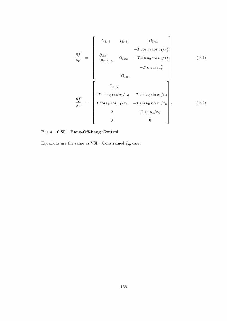
∂ ~f
∂~x=
O3×3 I3×3 O3×1
−T cosu0 cosu1/x26
∂aA∂x 3×3
O3×3 −T sinu0 cosu1/x26
−T sinu1/x26
O1×7
(164)
∂ ~f
∂~u=
O3×2
−T sinu0 cosu1/x6 −T cosu0 sinu1/x6
T cosu0 cosu1/x6 −T sinu0 sinu1/x6
0 T cosu1/x6
0 0
. (165)
B.1.4 CSI – Bang-Off-bang Control
Equations are the same as VSI – Constrained Isp case.
158
APPENDIX C
NUMERICAL TECHNIQUES
In this chapter, numerical techniques that are used to create an interplanetary trajectory
optimization program are introduced. These techniques are used to implement the methods
described in the last chapter into the program and they are as follows:
• A first-order gradient algorithm based on the optimal control technique is used to
compute the optimal control history of the thrust.
• Runge-Kutta integrates the equations of motion with a given initial condition. This
is used along with the first-order gradient algorithm.
• A line search is used with Powell’s method. Three-point quadratic polynomial ap-
proximations are used in this research.
• Powell’s method is a zero-order method that finds the minimum point. This is used
for several purposes:
– to find the best directions of motion of the spacecraft at departure and at arrival.
– to find the best entry velocity and the impact parameter for a swing-by trajectory.
– to find the initial values of the Lagrange multipliers that satisfy the target con-
ditions.
• Among several methods available to solve the Gauss problem that calculate a high
thrust trajectory, the direct p-iteration method is chosen. The procedure and equa-
tions for this method are introduced.
• Penalty functions are used for the trajectory inside the SOI for swing-by cases to
restrict the minimum approaching distance. As the spacecraft approaches the swing-
by planet, the spacecraft must not hit the planet or fly above the planet’s atmosphere
159
if there is an atmosphere.
This chapter also includes the brief explanation of VRML (Virtual Reality Modeling
Language).
C.1 Calculus of Variations: First-order Gradient Algorithm
Suppose that we would like to find the control variables u(t) on the time interval [ti, tf ] that
drive the plant
x = f [x(t), u(t), t], x(ti)given, ti ≤ t ≤ tf , (166)
along a trajectory x(t). x(t), an n-vector function, is determined by u(t), an m-vector func-
tion. The control history will be chosen such that the performance index, J , is minimized:
J = φ[x(tf ), tf ] +
∫ tf
ti
L[x(t), u(t), t] dt (167)
φ[x(tf ), tf ] : the final weighting function
L[x(t), u(t), t] : the Lagrangian
and such that the q-vector (q ≤ n− 1 if L = 0, q ≤ n if L 6= 0) side constraints ψ[x(tf ), tf ]
satisfy
ψ[x(tf ), tf ] = 0 (q equations). (168)
The computation method to obtain the histories of the control variables for the above
problem is presented below. This method is called the first-order gradient algorithm[17].
1. Estimate a set of control variable histories, u(t).
2. Integrate the system equations x = f(x, u, t) forward with the specified initial con-
ditions x(ti) and the control variable histories from Step 1. Record x(t), u(t), and
ψ[x(tf )].
3. Determine an n-vector of influence functions p(t), and an (n × q) matrix of influ-
ence functions, R(t), by backward integration of the influence equations, using x(tf )
160
obtained in Step 2 to determine the boundary conditions.
p = −(
∂f
∂x
)T
p−(
∂L
∂x
)T
; pi(tf ) =
0 i = 1, . . . , q,
(∂φ/∂xi)t=tf i = q + 1, . . . , n,
(169)
R = −(
∂f
∂x
)T
R; Rij(tf ) =
1, i = j, i = 1, . . . n,
0, i 6= j, j = 1, . . . q.
(170)
4. Simultaneously with Step 3, compute the following integrals:
Iψψ =
∫ tf
ti
RT∂f
∂uW−1
(
∂f
∂u
)T
Rdt [(q × q)-matrix] (171)
IJψ = ITψJ =
∫ tf
ti
(
pT∂f
∂u+∂L
∂u
)
W−1
(
∂f
∂u
)T
Rdt [q-row vector] (172)
IJJ =
∫ tf
ti
(
pT∂f
∂u+∂L
∂u
)
W−1
[
(
∂f
∂u
)T
p+
(
∂L
∂u
)T]
dt (173)
where W is an (m×m) positive-definite matrix and IJJ is a scalar.
5. Choose values of δψ such that the next nominal solution is closer to the desired values
ψ[x(tf )] = 0. For example, one might choose δψ = −εψ[x(tf )], 0 < ε ≤ 1. Then
determine ν from ν = −[Iψψ]−1(δψ + IψJ).
6. Repeat Steps 1 through 6, using an improved estimate of u(t), where
δu(t) = −[W (t)]−1
[
∂L
∂u+ [p(t) +R(t)ν]T
∂f
∂u
]T
. (174)
Stop when ψ[x(tf )] = 0 and IJJ − IJψI−1
ψψIψJ = 0 to the desired degree of accuracy.
The explicit forms of the derivatives (∂f/∂x), (∂L/∂x), (∂L/∂x), (∂L/∂u) are in Ap-
pendix B.1.
C.2 Numerical Integration: Runge-Kutta
The Runge-Kutta algorithm lets us solve a differential equation numerically. Consider a
single variable problem
y′ = f(x, y) (175)
161
with initial condition y(0) = y0. Suppose that yn is the value of the variable at xn. The
Runge-Kutta formula takes yn and xn and calculates an approximation for yn+1 at xn+1(=
xn + h, where h is assumed to be small).
For a second-order Runge-Kutta[11],
yn+1 = yn +h
2[f(xn, yn) + f(xn+1, yn + hf(xn, yn)] (176)
or
yn+1 = yn +h
2[F1 + F2] (177)
F1 = hf(xn, yn) (178)
F2 = hf(xn+1, yn + hf(xn, yn)) (179)
For a fourth-order Runge-Kutta,
yn+1 = yn +h
6[F1 + 2F2 + 2F3 + F4] (180)
F1 = f(xn, yn) (181)
F2 = f
(
xn +1
2h, yn +
1
2hF1
)
(182)
F3 = f
(
xn +1
2h, yn +
1
2hF2
)
(183)
F4 = f(xn + h, hn + hV3) (184)
C.3 Line Search: Three-point Polynomial Approximations
There are several line search methods. Golden Section Method[78] converges rapidly, but a
disadvantage is that the region where the minimum point lies should be known beforehand.
Most of the problems dealt with in this paper cannot use this method because there is
little information on the minimum points in these problems. In this research, three-point
polynomial approximations are used. This method can easily change the range and the
direction of the search vector. Therefore, this method is appropriate to the problems dealt
with in this research.
The second-order approximating polynomial is[78]
F = a0 + a1X + a2X2 (185)
162
For a three-point quadratic approximation, there are three known points: (X1, F1), (X2, F2),
and (X3, F3). From these points and Eqn. 185, coefficients a0, a1, a2 are obtained:
a0 = F1 − a1X1 − a2X21 (186)
a1 =F2 − F1
X2 −X1
− a2(X1 +X2) (187)
a2 =(F3 − F1)/(X3 −X1) − (F2 − F1)/(X2 −X1)
X3 −X2
. (188)
Assuming that the distance between X1 and X2 and between X2 and X3 are the same and
is expressed as dX, the value of X that minimizes the value of this polynomial is
X∗ = − a1
2a2
=4F2 − 3F1 − F3
4F2 − 2F3 − 2F1
dX. (189)
In the case where F1 > F2 > F3 or F1 < F2 < F3, that is, if the minimum does not
lie between X1 and X3, the accuracy of this polynomial approximation is questionable. In
such cases we can find a region where F2 is smaller than both F1 and F3 by either increasing
or decreasing the value of dX.
If the minimum does not exist between X1 and X3, the following steps are taken.
• If F1 > F2 > F3, it is likely that the minimum should lie a point beyond X3. By
doubling dX, the same search described above is repeated.
• If F1 < F2 < F3, the minimum is in the opposite direction. Change the search
direction by multiplying dX by -1, then repeat the same search.
C.4 Numerical Optimization: Powell’s Method
There are several types of methods for finding the minimum point of unconstrained prob-
lems. For example, first-order methods for finding the minimum utilize gradient information.
Examples of these methods are the steepest-decent method and Fletcher-Reeves method.
Second-order methods, such as Newton’s method, use gradients and the Hessian matrix and
usually converge faster than first-order methods. These gradient-based methods require the
calculation of the gradient of functions, but sometimes computing gradients is extremely
difficult or time-consuming, especially if the functions are complicated. Compared to these
163
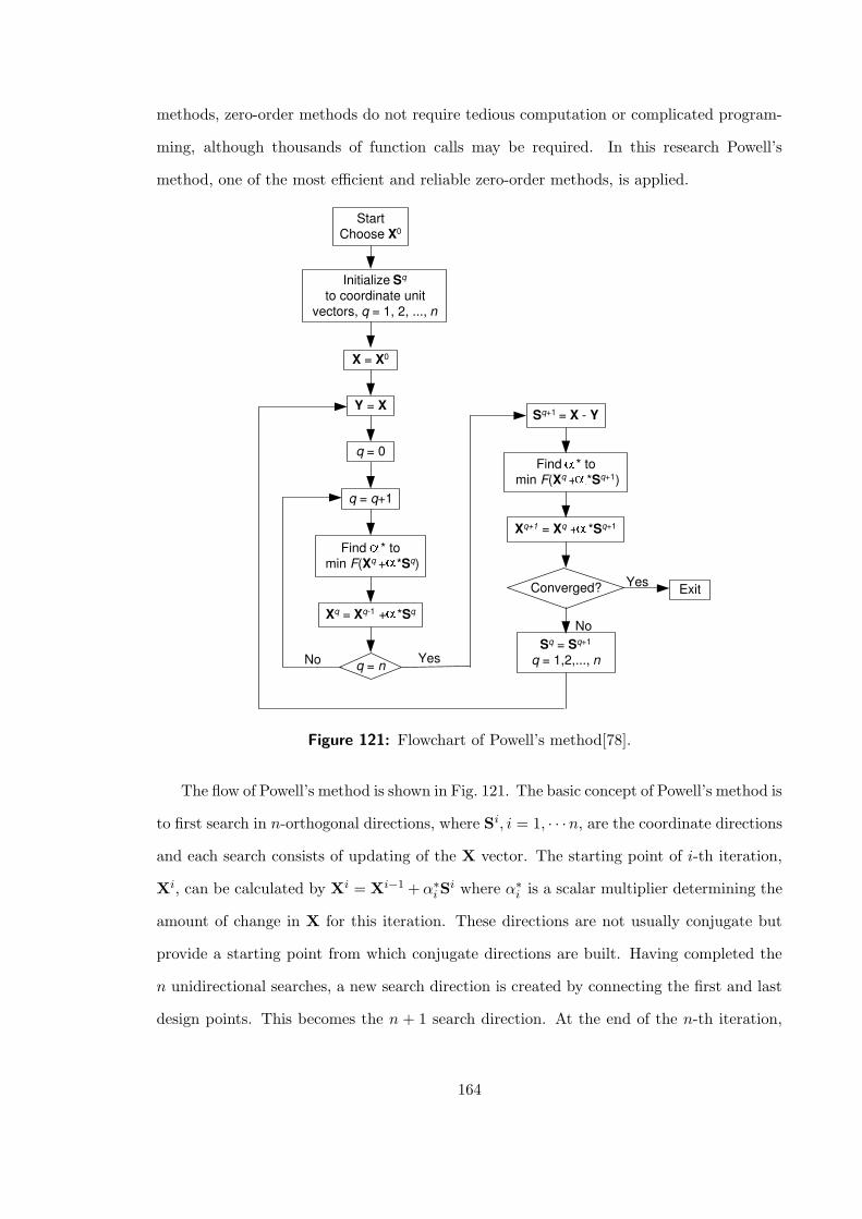
methods, zero-order methods do not require tedious computation or complicated program-
ming, although thousands of function calls may be required. In this research Powell’s
method, one of the most efficient and reliable zero-order methods, is applied.
Start Choose X 0
Initialize S q
to coordinate unit vectors, q = 1, 2, ..., n
X = X 0
Y = X
q = 0
q = q +1
Find * to min F ( X q + * S q )
X q = X q -1 + * S q
q = n
S q +1 = X - Y
Find * to min F ( X q + * S q +1 )
Converged?
X q+1 = X q + * S q +1
Exit Yes
No S q = S q +1
q = 1,2,..., n Yes No
Figure 121: Flowchart of Powell’s method[78].
The flow of Powell’s method is shown in Fig. 121. The basic concept of Powell’s method is
to first search in n-orthogonal directions, where Si, i = 1, · · ·n, are the coordinate directions
and each search consists of updating of the X vector. The starting point of i-th iteration,
Xi, can be calculated by Xi = Xi−1 +α∗
iSi where α∗
i is a scalar multiplier determining the
amount of change in X for this iteration. These directions are not usually conjugate but
provide a starting point from which conjugate directions are built. Having completed the
n unidirectional searches, a new search direction is created by connecting the first and last
design points. This becomes the n + 1 search direction. At the end of the n-th iteration,
164
the n+1-th search diretion Sn+1 is found by connecting all the points from X0 through the
point Xn.
Sn+1 =n∑
i=1
α∗
iSi (190)
It is convenient to store the search information in an n×n array H. Initially, the identity
matrix is used for this array. The columns of H correspond to the unidirectional search
vectors Si, i = 1 · · ·n. After finding the minimum in each direction, we replace Si in matrix
H by α∗
iSi.
H = [α∗
1S1 α∗
2S2 · · · α∗
nSn] (191)
For the n + 1-th search, we create a conjugate direction using Eqn. 190. With this search
vector the minimum point is calculated to determine the parameter α∗
i+1. Now each column
of the H matrix is shifted by one to the left, eliminating the α∗
1S1 entry, and storing
α∗
n+1Sn+1 in n-th column. This provides a new H matrix containing n search directions to
start the entire search process over. Therefore for this new search, the first search direction
is α∗
2S2.
Note that as the search goes on, the search directions may gradually become parallel. To
avoid the searches becoming stuck in the same direction, the H matrix should be periodically
reset to the identity matrix, in this case every 2n+ 1 iterations.
C.5 Solving High Thrust Problems: Gauss Problem
In this section, numerical method for solving Gauss problem is presented. The method used
in this research is “Solution via universal variables” explained in Sec. 5.3
C.5.1 Solution via Universal Variables
As explained above, this method requires the “direction of motion” to obtain ∆V . Following
this procedure:
1. From ~r1 and ~r2 and the “direction of motion,” evaluate the constant, A, using
A =
√r1r2 sin ∆ν√1 − cos ∆ν
(192)
165
where ∆ν is obtained from
∆ν = arccos
(
~r1 · ~r2|~r1||~r2|
)
. (193)
2. Pick a trial value for z. Since z = ∆E2 and −z = ∆F 2, this amounts to guessing
the change in the eccentric anomaly. The usual range for z is from negative values to
(2π)2. Values of z greater than (2π)2 correspond to a change in the eccentric anomaly
of more than 2π and can occur only if the satellite passes back through ~r1 enroute to
~r2.
3. Evaluate the functions S and C for the selected trial value of z using the following
equations.
C(z) ≡ 1 − cos√z
z=
1 − cosh√−z
z=
1
2!− z
4!+z2
6!− z3
8!+ . . .
=∞∑
k=0
(−z)k(2k + 2)!
(194)
S(z) ≡√z − sin
√z√
z3=
sinh√−z −
√−z
√
(−z)3=
1
3!− z
5!+z2
7!− z3
9!+ . . .
=
∞∑
k=0
(−z)k(2k + 3)!
. (195)
4. Determine the auxiliary variable, y, from
y = r1 + r2 −A(1 − zS)√
C. (196)
5. Determine x from
x =
√
y
C. (197)
6. Check the trial value of z by computing t from the equation
õt = x3S +A
√y (198)
and compare it with the desired time of flight. If the two values are not nearly equal,
adjust the trial value of z and repeat the procedure until the desired value of t is
obtained. A Newton iteration is typically used to calculate next value of z.
zn+1 = zn +t− tn
dt/dz|z=zn
(199)
166
where
õdt
dz= x3
(
S′ − 3SC ′
2C
)
+A
8
(
3S√y
C+A
x
)
. (200)
S′ and C ′ are the derivatives of S and C with respect to z. These derivatives may be
evaluated from these equations except when z is nearly zero (near-parabolic orbit).
dS
dz=
1
2z(C − 3S) (201)
dC
dz=
1
2z(1 − zS − 2C). (202)
If z is near zero, these equations may be used.
C ′ = − 1
4!+
2z
6!− 3z2
8!+
4z3
10!− . . . (203)
S′ = − 1
5!+
2z
7!− 3z2
9!+
4z3
11!− . . . (204)
7. When the method has converged to a solution, evaluate f , g, and g from Eqns. 97,
98, and 100, then compute ~v1 and ~v2 from
~v1 =~r2 − f~r1
g(205)
~v2 =g~r2 − ~r1
g. (206)
When ∆ν = π, the Gauss problem cannot be solved because two collinear vectors cannot
determine a unique orbital plane and therefore a unique solution for ~v1 and ~v2 is not possible.
In such a case, ∆V is calculated in the same way as the ∆V for a Hohmann transfer.
The semi-major axis of the transfer orbit is a = (r1 + r2)/2, and the specific energy is
E = −µ/(2a). The speeds at r1 and r2 are
V1 =
√
2
(
E +µ
r1
)
(207)
V2 =
√
2
(
E +µ
r2
)
(208)
Although the magnitude of the velocity is defined by the above equations, the velocity of the
spacecraft can be freely chosen. SAMURAI calculates the departure and arrival velocities
167
so that the total ∆V is minimized. The components of these velocities are adjusted with
Powell’s method until the following value is minimized:
total ∆V =√
(u(ti) − uinitial)2 + (v(ti) − vinitial)2 + (w(ti) − winitial)2
+√
(u(tf ) − utarget)2 + (v(tf ) − vtarget)2 + (w(tf ) − wtarget)2 (209)
where uinitial, vinitial, winitial are the velocity components of the departure planet, and
utarget, vtarget, and wtarget are the velocity components of the arrival planet.
C.6 Solving Swing-by Problems
A trajectory with a swing-by is solved based on the method shown previously(Sec.5.4).
Assume that we know the following numbers from the inputs: initial position and ve-
locity of the spacecraft, position of the swing-by planet, target position and velocity of the
spacecraft, times of flight for two phases (initial planet to swing-by planet, swing-by planet
to target planet). We would like to find the best thrust history that minimizes the fuel
consumption over an entire trajectory. Then we need to find the best velocity vector of
the spacecraft at the entrance of the SOI of the swing-by planet that minimizes the fuel
consumption. Once we set this velocity, fuel consumption for each phase can be solved.
Therefore, the velocity components are the parameters that we need to optimize. In ad-
dition, the impact parameter β determines the trajectory’s characteristics. Powell’s method
is used for the optimization to minimize the fuel consumption by changing these four pa-
rameters: u, v, w, and β.
Intuitively, Powell’s method is appropriate for this type of problem because there is only
one possible solution for the combination of u, v, w, and β. However, Powell’s method is
valid only for an unconstrained problem. As shown in Eqn. 128, there is a restriction on β
such that the spacecraft will not be decelerated by the atmosphere of the swing-by planet.
To deal with a constrained problem, while still using Powell’s method, a method of
penalty function is used.
168
C.6.1 Penalty Functions
The general approach for constrained minimization problems is to minimize the objec-
tive function as an unconstrained function but to add some penalty to limit constraint
violations[78]. The common approach is to create a pseudo-objective function of the form
Φ(X, k) = F (X) + kP (X) (210)
where F (X) is the original objective function and P (X) is an imposed penalty function.
The scalar k is a multiplier which determines the magnitude of the penalty, and k is held
constant for a complete unconstrained minimization. There are several types of penalty
functions[78].
C.6.1.1 Exterior Penalty Functions
This type of penalty function is the easiest to incorporate into the optimization process.
The exterior penalty function P (X) is given by
P (X) =m∑
i=1
max[0, gj(X)]2 +l∑
k=1
[hk(X)]2 (211)
This means that no penalty is imposed if all constraints are satisfied(all gj(X) ≤ 0
and all hk(X) = 0), but whenever one or more constraints are violated, the square of this
constraint is included in the penalty function.
We usually start with a small k and minimize Φ(X, k). Then increase k by a factor of
γ, for example γ = 3, and minimize Φ again. This process continues until a satisfactory
result is obtained.
The disadvantage of the exterior penalty function is that it begins from an infeasible
region, and the solution becomes feasible only in the limit as k → ∞. Therefore, if the
optimization process is stopped prematurely, the result is unusable.
C.6.1.2 Interior Penalty Functions
Unlike exterior penalty functions, interior penalty functions start within the feasible region,
and even if the optimization is prematurely stopped, the design will at least be feasible,
even though it may not be optimum.
169
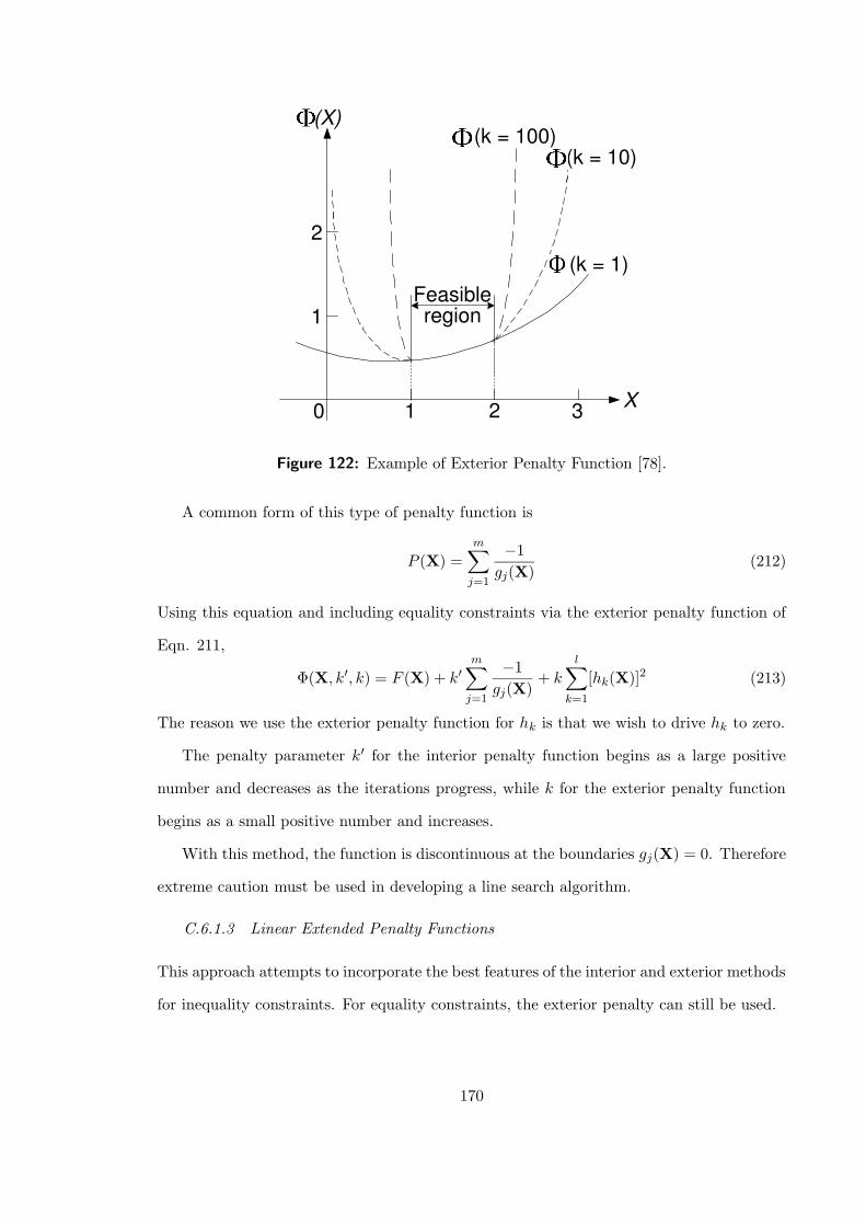
X 1 3 2
1
2
Feasible region
0
(X) (k = 100)
(k = 10)
(k = 1)
Figure 122: Example of Exterior Penalty Function [78].
A common form of this type of penalty function is
P (X) =m∑
j=1
−1
gj(X)(212)
Using this equation and including equality constraints via the exterior penalty function of
Eqn. 211,
Φ(X, k′, k) = F (X) + k′m∑
j=1
−1
gj(X)+ k
l∑
k=1
[hk(X)]2 (213)
The reason we use the exterior penalty function for hk is that we wish to drive hk to zero.
The penalty parameter k′ for the interior penalty function begins as a large positive
number and decreases as the iterations progress, while k for the exterior penalty function
begins as a small positive number and increases.
With this method, the function is discontinuous at the boundaries gj(X) = 0. Therefore
extreme caution must be used in developing a line search algorithm.
C.6.1.3 Linear Extended Penalty Functions
This approach attempts to incorporate the best features of the interior and exterior methods
for inequality constraints. For equality constraints, the exterior penalty can still be used.
170
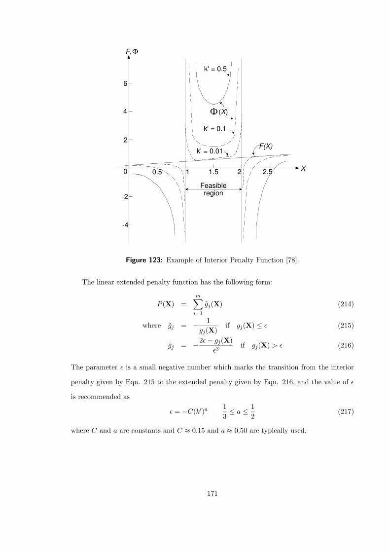
6
4
2
0
-2
-4
0.5 1 1.5 2 2.5 X
Feasible region
k' = 0.5
k' = 0.1
k' = 0.01
F ,
( X )
F(X)
Figure 123: Example of Interior Penalty Function [78].
The linear extended penalty function has the following form:
P (X) =m∑
i=1
gj(X) (214)
where gj = − 1
gj(X)if gj(X) ≤ ε (215)
gj = −2ε− gj(X)
ε2if gj(X) > ε (216)
The parameter ε is a small negative number which marks the transition from the interior
penalty given by Eqn. 215 to the extended penalty given by Eqn. 216, and the value of ε
is recommended as
ε = −C(k′)a1
3≤ a ≤ 1
2(217)
where C and a are constants and C ≈ 0.15 and a ≈ 0.50 are typically used.
171
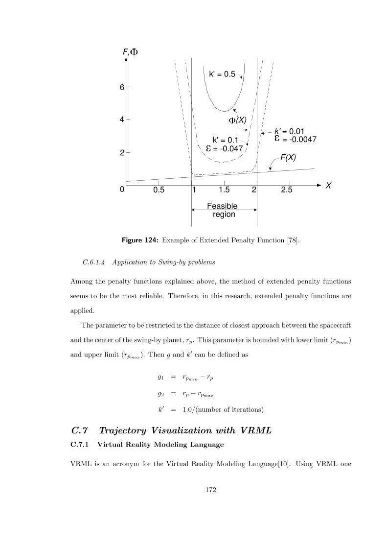
6
4
2
0 0.5 1 1.5 2 2.5 X
Feasible region
k' = 0.5
k' = 0.1 k' = 0.01
F(X)
F,
(X)
= -0.047 = -0.0047
Figure 124: Example of Extended Penalty Function [78].
C.6.1.4 Application to Swing-by problems
Among the penalty functions explained above, the method of extended penalty functions
seems to be the most reliable. Therefore, in this research, extended penalty functions are
applied.
The parameter to be restricted is the distance of closest approach between the spacecraft
and the center of the swing-by planet, rp. This parameter is bounded with lower limit (rpmin)
and upper limit (rpmax). Then g and k′ can be defined as
g1 = rpmin− rp
g2 = rp − rpmax
k′ = 1.0/(number of iterations)
C.7 Trajectory Visualization with VRML
C.7.1 Virtual Reality Modeling Language
VRML is an acronym for the Virtual Reality Modeling Language[10]. Using VRML one
172
can craft three-dimensional virtual worlds on the internet. With a text file as an input file,
VRML draws many types of objects as well as animations.
In this research, the trajectory is drawn with VRML for easy visualization. SAMURAI
outputs a file that is used as a VRML input file. A three dimensional trajectory is drawn on
a web browser with the thrust direction vectors shown at several points along the trajectory.
It is sometimes difficult to choose the departure date or time of flight. If a user chooses
a bad combination of these two values, the calculation will not converge. Because this
drawing displays the positions of departure and arrival planets, it is helpful to determine
when to depart and what time of flight to choose.
C.7.2 Input and Output in General
Several simple examples shown introduce how VRML works.
A VRML input file must start with the line
#VRML V2.0 utf8
The following very simple file sphere.wrl draws a sphere with a radius of 1.0 with its centerat the origin.
#VRML V2.0 utf8 Sphere
A red cone with a bottom radius of 2.0 and a height of 3.0 is:
#VRML V2.0 utf8 Shape appearance Appearance
material Material emissiveColor 1 0 0 # red=1 green=0 blue=0
geometry Cone
bottomRadius 2.0height 3.0
Comment lines can be written beginning with “#” except for the first line. By grouping
a cone and a cylinder, we can make a simple house as shown in Fig. 125. We need to move
either a cone or a cylinder with the translation command because all of the shapes are
drawn with its center at the origin unless otherwise specified.
#VRML V2.0 utf8 Group children [
Shape appearance Appearance
material Material emissiveColor 0 0 1 # blue
173
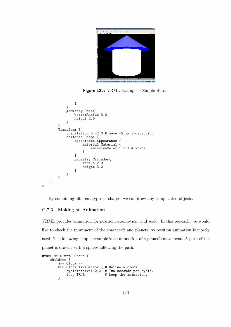
Figure 125: VRML Example – Simple House.
geometry Cone
bottomRadius 3.0height 2.0
Transform
translation 0 -2 0 # move -2 in y-directionchildren Shape
appearance Appearance material Material
emissiveColor 1 1 1 # white
geometry Cylinder
radius 2.0height 3.0
]
By combining different types of shapes, we can draw any complicated objects.
C.7.3 Making an Animation
VRML provides animation for position, orientation, and scale. In this research, we would
like to check the movement of the spacecraft and planets, so position animation is mostly
used. The following simple example is an animation of a planet’s movement. A path of the
planet is drawn, with a sphere following the path.
#VRML V2.0 utf8 Group children [
#== Clock ==DEF Clock TimeSensor # Define a clock.
cycleInterval 2.0 # Two seconds per cycle.loop TRUE # Loop the animation.
174
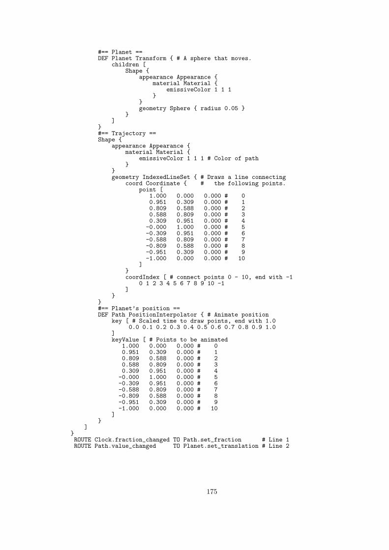
#== Planet ==DEF Planet Transform # A sphere that moves.
children [Shape
appearance Appearance material Material
emissiveColor 1 1 1
geometry Sphere radius 0.05
]
#== Trajectory ==Shape
appearance Appearance material Material
emissiveColor 1 1 1 # Color of path
geometry IndexedLineSet # Draws a line connecting
coord Coordinate # the following points.point [
1.000 0.000 0.000 # 00.951 0.309 0.000 # 10.809 0.588 0.000 # 20.588 0.809 0.000 # 30.309 0.951 0.000 # 4-0.000 1.000 0.000 # 5-0.309 0.951 0.000 # 6-0.588 0.809 0.000 # 7-0.809 0.588 0.000 # 8-0.951 0.309 0.000 # 9-1.000 0.000 0.000 # 10
]coordIndex [ # connect points 0 - 10, end with -1
0 1 2 3 4 5 6 7 8 9 10 -1]
#== Planet’s position ==DEF Path PositionInterpolator # Animate position
key [ # Scaled time to draw points, end with 1.00.0 0.1 0.2 0.3 0.4 0.5 0.6 0.7 0.8 0.9 1.0
]keyValue [ # Points to be animated
1.000 0.000 0.000 # 00.951 0.309 0.000 # 10.809 0.588 0.000 # 20.588 0.809 0.000 # 30.309 0.951 0.000 # 4-0.000 1.000 0.000 # 5-0.309 0.951 0.000 # 6-0.588 0.809 0.000 # 7-0.809 0.588 0.000 # 8-0.951 0.309 0.000 # 9-1.000 0.000 0.000 # 10
]
]ROUTE Clock.fraction_changed TO Path.set_fraction # Line 1ROUTE Path.value_changed TO Planet.set_translation # Line 2
175
The last two lines (Line 1 and Line 2) make the animation work. VRML checks the
clock of the computer, and the clock information is brought to TimeSensor that induces
the change of fraction of Clock. The change of fraction (Clock.fraction changedin
Line 1) is routed to PositionInterpolator, which is defined as Path, and sets the fraction
of Path. Setting the fraction is notified to Line 2 as the change of value in Path, and
this information is routed to Planet. Planet then draws a sphere to the coordinates (or
keyValue) specified by Path. These two lines are looped and a sphere is drawn according
to the coordinates specified at keyValue, resulting in an animation of a moving sphere.
176
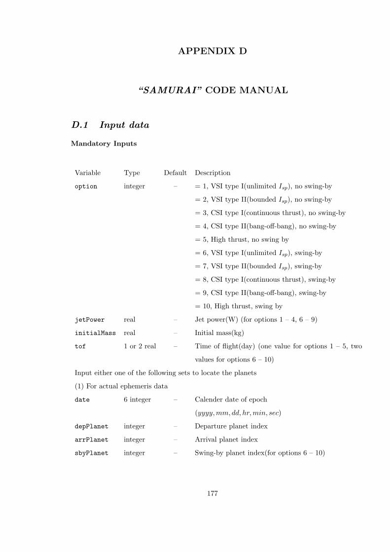
APPENDIX D
“SAMURAI” CODE MANUAL
D.1 Input data
Mandatory Inputs
Variable Type Default Description
option integer – = 1, VSI type I(unlimited Isp), no swing-by
= 2, VSI type II(bounded Isp), no swing-by
= 3, CSI type I(continuous thrust), no swing-by
= 4, CSI type II(bang-off-bang), no swing-by
= 5, High thrust, no swing by
= 6, VSI type I(unlimited Isp), swing-by
= 7, VSI type II(bounded Isp), swing-by
= 8, CSI type I(continuous thrust), swing-by
= 9, CSI type II(bang-off-bang), swing-by
= 10, High thrust, swing by
jetPower real – Jet power(W) (for options 1 – 4, 6 – 9)
initialMass real – Initial mass(kg)
tof 1 or 2 real – Time of flight(day) (one value for options 1 – 5, two
values for options 6 – 10)
Input either one of the following sets to locate the planets
(1) For actual ephemeris data
date 6 integer – Calender date of epoch
(yyyy,mm, dd, hr,min, sec)
depPlanet integer – Departure planet index
arrPlanet integer – Arrival planet index
sbyPlanet integer – Swing-by planet index(for options 6 – 10)
177
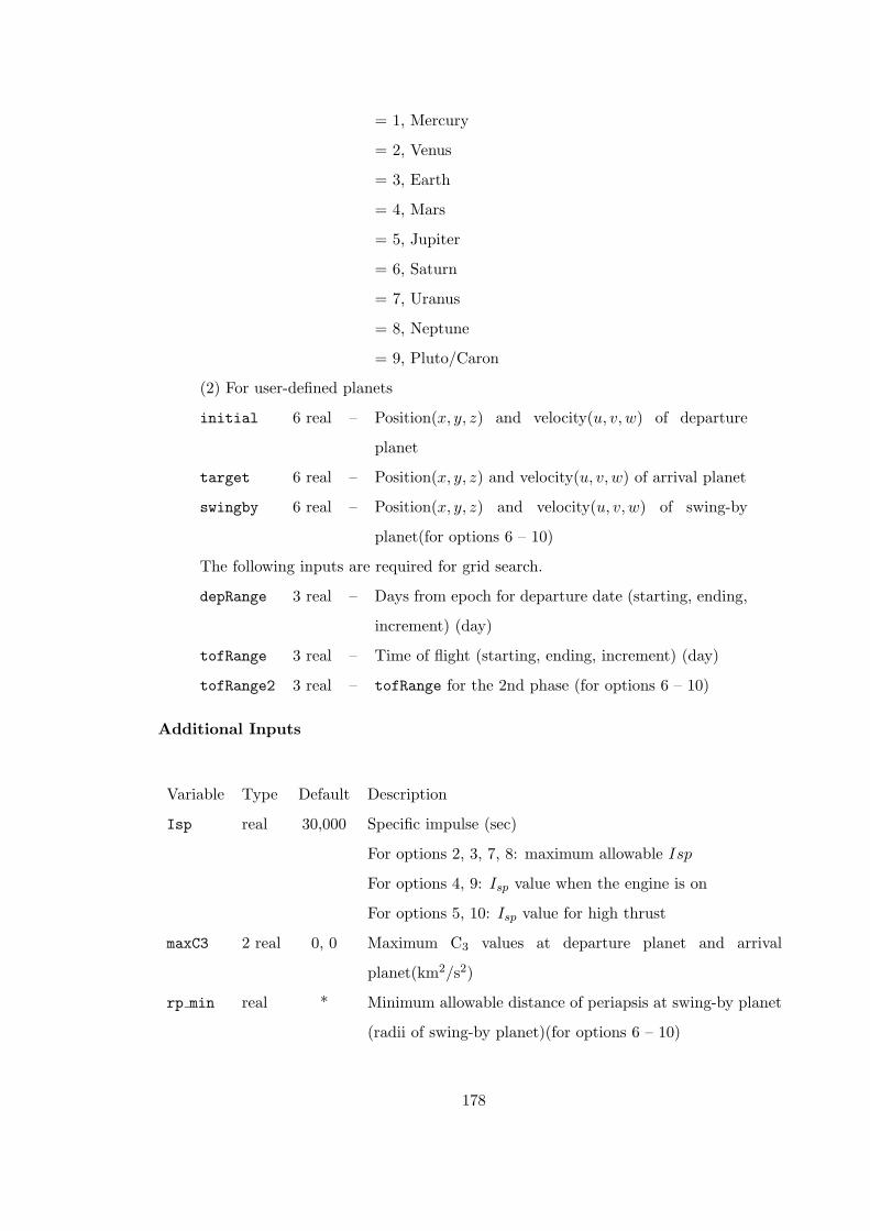
= 1, Mercury
= 2, Venus
= 3, Earth
= 4, Mars
= 5, Jupiter
= 6, Saturn
= 7, Uranus
= 8, Neptune
= 9, Pluto/Caron
(2) For user-defined planets
initial 6 real – Position(x, y, z) and velocity(u, v, w) of departure
planet
target 6 real – Position(x, y, z) and velocity(u, v, w) of arrival planet
swingby 6 real – Position(x, y, z) and velocity(u, v, w) of swing-by
planet(for options 6 – 10)
The following inputs are required for grid search.
depRange 3 real – Days from epoch for departure date (starting, ending,
increment) (day)
tofRange 3 real – Time of flight (starting, ending, increment) (day)
tofRange2 3 real – tofRange for the 2nd phase (for options 6 – 10)
Additional Inputs
Variable Type Default Description
Isp real 30,000 Specific impulse (sec)
For options 2, 3, 7, 8: maximum allowable Isp
For options 4, 9: Isp value when the engine is on
For options 5, 10: Isp value for high thrust
maxC3 2 real 0, 0 Maximum C3 values at departure planet and arrival
planet(km2/s2)
rp min real * Minimum allowable distance of periapsis at swing-by planet
(radii of swing-by planet)(for options 6 – 10)
178
rp max real * Maximum allowable distance of periapsis at swing-by planet
(radii of swing-by planet)(for options 6 – 10)
rSOI sby real 9.245E+05 SOI radius of swing-by planet (km) (for options 6 – 10)
TU sby real 806.812 Time unit of swing-by planet (sec) (for options 6 – 10)
DU sby real 6378.145 Distance unit of swing-by planet (km) (for options 6 – 10)
Optional Inputs
Variable Type Default Description
timeSteps 1 or 2 100, Number of time steps for each leg (one value for
integer 100 options 1 – 5, two values for options 6 – 10)
max ite integer 300 Maximum number of iterations for optimal control process
D.2 Executing “SAMURAI”
SAMURAI reads an input data file (e.g. INPUT.txt) and the results are written to an
output data file (e.g. OUTPUT.txt). A VRML file (e.g. VRML.wrl) is also created. Users
must specify these three files from the command line.
> samurai INPUT.txt OUTPUT.txt VRML.wrl
The computation time strongly depends on the option (option) and the number of time
steps (timeSteps). If the number of time steps is 300, approximate computation time with
Pentium 4, 1.9GHz for each option is: less than 10 sec for option 1, less than a few minutes
for option 2, less than 10 minutes for option 3 and 4, and less than 1 sec for option 5.
It is not recommended to conduct a grid search for swing-by trajectories with CSI
engines with a wide search range because it may take very long time to complete.
179

REFERENCES
[1] “A Crewed Mission to Mars....”http://nssdc.gsfc.nasa.gov/planetary/mars/marswhy.html.
[2] “EICR Plasma Propulsion Systems at Kyushu University, Japan.”http://art.aees.kyushu-u.ac.jp/members/yositaka/study/doc/japanese/research-j.html.
[3] “Jupiter Icy Moons Orbiter.” http://www.jpl.nasa.gov/jimo/index.cfm.
[4] “Spacecraft Propulsion – Wikipedia, the free encyclopedia.”http://en.wikipedia.org/wiki/Spacecraft propulsion.
[5] “Superfast VASIMR Rocket in Funding Limbo.”http://www.space.com/businesstechnology/technology/vasimr rocket 020807-1.html.
[6] “The Exploration of Jupiter in the 21st Century.”http://www.vectorsite.net/taxpl b.htm.
[7] “Variable-Specific-Impulse Magnetoplasma Rocket.”http://www.nasatech.com/Briefs/Sep01/MSC23041.html.
[8] Akulenko, L. D., Problems and Methods of Optimal Control, vol. 286 of Mathematics
and Its Applications. Dordrecht, The Netherlands: Kluwer Academic Publishers, 2003.
[9] Alperin, M. and Gregory, H. F., Vistas in Astronautics, vol. 2. New York: Perg-amon Press, 1959.
[10] Ames, A. L., Nadeau, D. R., and Moreland, J. L., VRML 2.0 Sourcebook Second
Edition. New York, NY: John Wiley & Sons, Inc., 1997.
[11] Atkinson, K. E., An Introduction to Numerical Analysis, Second Edition. New York,NY: John Wiley & Son, 1989.
[12] Bate, R. R., Mueller, D. D., and E.White, J., Fundamentals of Astrodynamics.New York, NY: Dover Publications, Inc., 1971.
[13] Battin, R. H., An Introduction to the Mathematics and Methods of Astrodynamics,
Revised Edition. AIAA Education Series, Reston, VA: American Institute of Aeronau-tics and Astronautics, Inc., 1999.
[14] Broucke, R. A. and Prado, A. F. B. A., “Optimal N-Impulse Transfer BetweenCoplanar Orbits,” Advances in the Astronautical Sciences, Astrodynamics 1993, vol. 85,pp. 483–502, 1993. AAS93-660.
[15] Bryson, Jr., A., Denham, W., and Dreyfus, S., “Optimal Programming Problemswith Inequality Constraints I: Necessary Conditions for Extremal Solutions,” AIAA
Journal, vol. 1, pp. 2544 – 2550, Nov. 1963.
180
[16] Bryson, Jr., A., Denham, W., and Dreyfus, S., “Optimal Programming Probelmswith Inequality Constraints II: Solution by Steepest-Ascent,” AIAA Journal, vol. 2,pp. 25 – 34, Jan. 1964.
[17] Bryson, Jr., A. E. and Ho, Y.-C., Applied Optimal Control. Bristol, PA: Taylor &Francis, 1975.
[18] Carey, R. and Bell, G., The Annotated VRML 2.0 Reference Manual. Boston, MA:Addison-Wesley, 1997.
[19] Casalino, L., Colasurdo, G., and Pastrone, D., “Optimization of ∆V Earth-Gravity-Assist Trajectories,” Journal of Guidance, Control, and Dynamics, vol. 21,no. 6, pp. 991–995, 1998.
[20] Casalino, L., Colasurdo, G., and Pastrone, D., “Optimal Low-Thrust EscapeTrajectories Using Gravity Assist,” Journal of Guidance, Control, and Dynamics,vol. 22, no. 5, pp. 638–642, 1999.
[21] Casalino, L., Colasurdo, G., and Pastrone, D., “Simple Strategy for PoweredSwingby,” Journal of Guidance, Control, and Dynamics, vol. 22, no. 1, pp. 156–159,1999.
[22] Chang-Diaz, F. R., “An Overview of the VASIMR Engine: High Power Space Propul-sion with RF Plasma Generation and Heating.” 14th Topical Conference on RadioFrequency Power in Plasmas, Oxnard, California, May 7-9, 2001.
[23] Chang-Diaz, F. R., “The VASIMR Rocket,” Scientific American, pp. 91–97, Nov.2000.
[24] Chang-Diaz, F. R., Bengston, R. D., Breizman, B. N., and Baity, F. W., “Thephysics and Engineering of the VASIMR Engine.” 36th AIAA/ASME/SAE/ASEEJoint Propulsion Conference Huntsville, Alabama, July 17-19 2000.
[25] Chang-Diaz, F. R., Hsu, M. M., Braden, E., Johnson, I., and Yang, T. F.,“Rapid Mars Transits With Exhaust-Modulated Plasma Propulsion,” NASA TechnicalPaper 3539, NASA, 1995.
[26] Chang-Diaz, F. R., Squire, J. P., Ilin, A., Nguyen, T., Winer, D., Petro, A.,Goebel, G., Cassady, L., Stokke, K., Dexter, C., Graves, T., Jr., L. A., andGeorge, J., “The Development of the VASIMR Engine.”
[27] Chobotov, V. A., Orbital Mechanics Second Edition. AIAA Education Series, Re-ston, VA: American Institute of Aeronautics and Astronautics, Inc., 1996.
[28] de Almeida Prado, A. F. B., “Powered Swingby,” Journal of Guidance, Control,
and Dynamics, vol. 19, no. 5, pp. 1142–1147, 1996.
[29] Dickey, B., “Star Power,” Air & Space, pp. 64–67, 2004.
[30] E.A.Bering, I., Brukardt, M., Chang-Diaz, F. R., Squire, J., Jacobson, V.,Bengtson, R. D., J.N.Gibson, and T.W.Glover, “Experimental Studies of theExhaust Plasma of The VASIMR Engine.” 40th AIAA Aerospace Sciences Meeting &Exhibit, Reno, NV, January 14-17 2002. AIAA2002-0345.
181
[31] Escobal, P. R., Methods of Orbit Determination. New York: John Wiley & Sons,Inc., 1965.
[32] Escobal, P. R., Methods of Astrodynamics. New York: John Wiley and& Sons, Inc.,1968.
[33] Goodson, T., Fuel-Optimal Control and Guidance for Low- and Medium-Thrust Or-
bit Transfer. PhD dissertation, Georgia Institute of Technology, School of AerospaceEngineering, Aug. 1995.
[34] Griffin, M. D. and French, J. R., Space Vehicle Design. AIAA Education Series,Washington, DC: American Institute of Aeronautics and Astronautics, Inc., 1991.
[35] Hack, K. J., George, J. A., and Dudzinski, L. A., “Nuclear Electric PropulsionMission Performance for Fast Piloted Mars Missions,” AIAA Paper 91-3488, AIAA,Sept. 1991.
[36] Hack, K. J., George, J., Riehl, J., and Gilland, J. H., “Evolutionary Use ofNuclear Electric Propulsion,” AIAA Paper 90-3821, AIAA, Sept. 1990.
[37] Hale, F. J., Introduction to Space Flight. Englewood Cliffs, NJ: Prentice-Hall, Inc.,1994.
[38] Hill, P. and Peterson, C., Mechanics and Thermodynamics of Propulsion Second
Edition. Reading, MA: Addison-Wesley Publishing Company, 1992.
[39] Holzner, S., Perl Core Language. Little Black Book, Scottsdale, AZ: Coriolis Tech-nology Press, 1999.
[40] Hong, P., Kent, P., Olson, D., and Vallado, C., “Interplanetary Program ToOptimize Simulated Trajectories (IPOST) User’s Guide,” Oct. 1992. NAS1-18230.
[41] Hull, D. G., Optimal Control Theory for Applications. Mechanical Engineering Series,New York, NY: Springer, 2003.
[42] Humble, R. W., Henry, G. N., and Larson, W. J., Space Propulsion Analysis and
Design. Space Technology Series, New York, NY: The MacGraw-Hill Companies, Inc.,1995.
[43] Ilin, A., Chang-Diaz, F. R., Squire, J., Breizman, B., and Carter, M., “Parti-cle Simulations of Plasma Heating in VASIMR.” 36th AIAA/ASME/SAE/ASEE JointPropulsion Conference Huntsville, Alabama, July 17-19 2000. AIAA2000-3753.
[44] Ilin, A., Chang-Diaz, F. R., Squire, J., Tarditi, A., B.N.Breizman,and M.D.Carter, “Simulations of Plasma Detachment in VASIMR.” 40th AIAAAerospace Sceinces Meeting & Exhibit, Reno, NV, January 14-17 2002. AIAA2002-0346.
[45] Jacobson, V. T., Diaz, F. R. C., Squire, J. P., McCaskill, G. E., McCoy,
J. E., Petro, A. J., Winter, D. S., and Jamison, H. M., “Development of VASIMRHelicon Source.” 43rd Annual Meeting of the APS Division of Plasma Physics Mini-Conference on Helicon Sources, Long Beach, California.
182
[46] Kahler, S., Lu, P., and Hanson, J., “Optimal Interplanetary Trajectories Using anAdvanced Pulsed Fusion Propulsion System.” AAS03-571, AAS/AIAA Astrodynamicsspecialists Conference, Big Sky Resort, Big Sky, Montana, August 3–7, 2003.
[47] Kechichian, J. A., “Trajectory Optimization Using Eccentric Longitude Formula-tion,” Advances in the Astronautical Sciences, Astrodynamics 1993, vol. 85, pp. 543–562, 1993. AAS93-664.
[48] Kechichian, J. A., “Mechanics of Trajectory Optimization Using Nonsingular Varia-tional Equations in Polar Coordinates,” Advances in the Astronautical Sciences, Space-
flight Mechanics 1995, vol. 89, pp. 937–958, 1995. AAS95-121.
[49] Kechichian, J. A., “Optimal Low-Thrust Transfer Using Variable Bounded Thrust,”Acta Astronautica, vol. 36, no. 7, pp. 357–365, 1995.
[50] Kechichian, J. A., “Trajectory Optimization Using Nonsingular Orbital Elementsand True Longitude,” Advances in the Astronautical Sciences, Astrodynamics 1995,vol. 90, pp. 1793–1814, 1995. AAS95-422.
[51] Kluever, C. A. and Pierson, B. L., “Optimal low-thrust three-dimensional earth-moon trajectories,”
[52] Kluever, C. A. and Pierson, B. L., “Optimal Earth-Moon Trajectories UsingNuclear Electric Propulsion,” Advances in the Astronautical Sciences, Astrodynamics
1995, vol. 90, pp. 1623–1638, 1995.
[53] Labunsky, A. V., Papkov, O. V., and Sukhanov, K. G., Multiple Gravity Assist
Interplanetary Trajectories, vol. 3 of Earth Space Institute Book Series. Amsterdam,The Netherlands: Gordon and Breach Science Publishers, 1998.
[54] Lawden, D. F., Optimal Trajectories for Space Navigation. London: Butterworths,1963.
[55] Ledsinger, L. A., Solutions to Decomposed Branching Trajectories with Powered Fly-
back Using Multidisciplinary Design Optimization. PhD dissertation, Georgia Instituteof Technology, School of Aerospace Engineering, July 2000.
[56] Leitmann, G., The Calculus of Variations and Optimal Control, vol. 24 of Mathemat-
ical Concepts and Methods in Science and Engineering. New York, NY: Plenum Press,1981.
[57] Lewis, F. L., Optimal Control. New York, NY: John Wiley & Sons, Inc., 1986.
[58] marc R. Ilgen, “Low Thrust OTV Guidance Using Lyapunov Optimal Feedback Con-trol,” Advances in the Astronautical Sciences, Astrodynamics 1993, vol. 85, pp. 1527–1545, 1993. AAS93-680.
[59] Marec, J.-P., Optimal Space Trajectories, vol. 1 of Studies in Astronautics. Amster-dam, The Netherlands: Elsevier Scientific Publishing Company, 1979.
[60] Miele, A., Wang, T., and Mancuso, S., “Optimal Free-Return Trajectories forMoon Missions and Mars Missions,” Advances in the Astronautical Sciences, The
Richard H. Battin Astrodynamics Symposium 2000, vol. 106, pp. 93–115, 2000. AAS00-254.
183
[61] Nah, R. and Vadali, S., “Fuel-Optimal, Low-Thrust Three-Dimensional Earth-MarsTrajectories,” Journal of Guidance, Control, and Dynamics, vol. 24, no. 6, pp. 1100–1107, 2001.
[62] Ocampo, C. A., “Trajectory Optimization with Dual Thrust Limited Propulsion Sys-tems,” Advances in the Astronautical Sciences, Astrodynamics 2001, vol. 109, pp. 2015–2032, 2001. AAS01-443.
[63] Ocampo, C. A. and Rosborough, G. W., “Optimal Low-Thrust Transfers Betweena Class of Restricted Three-Body Trajectories,” Advances in the Astronautical Sciences,
Astrodynamics 1993, vol. 85, pp. 1547–1566, 1993. AAS93-681.
[64] Pastrone, D., Casalino, L., and Colasurdo, G., “Indirect Optimization Methodfor Round-Trip Mars Trajectories,” Advances in the Astronautical Sciences, Astrody-
namics 1995, vol. 90, pp. 85–99, 1995. AAS95-305.
[65] Petro, A., Chang-Diaz, F. R., Carter, M. D., Schwenterly, S., Hitt,
M., and Lepore, J., “A Flight Demonstration of Plasma Rocket Propulsion.” 36thAIAA/ASME/SAE/ASEE Joint Propulsion Conference Huntsville, Alabama, July 17-19 2000. AIAA2000-3751.
[66] Petro, A., Chang-Diaz, F. R., Ilin, A., and Squire, J., “Development of aSpace Station-Based Flight Experiment for the VASIMR Magneto-Plasma Rocket.”40th AIAA Aerospace Sciences Meeting & Exhibit, Reno, NV, January 14-17 2002.AIAA2002-0344.
[67] Pierson, B. L. and Kluever, C. A., “A Three-Stage Approach to Optimal Low-Thrust Earth-Moon Trajectories,” Advances in the Astronautical Sciences, Astrody-
namics 1993, vol. 85, pp. 563–582, 1993.
[68] Press, W. H., Teukolsky, S. A., Vetterling, W. T., and Flannery, B. P., Nu-
merical Recipes in C – The Art of Scientific Computing – Second Edition. Cambridge:Cambridge University Press, 1988.
[69] Ranieri, C. L. and Ocampo, C. A., “Optimization of Roundtrip, Time-Constrained,Finite Burn Trajectories Via an Indirect Method.” AAS03-572, AAS/AIAA Astrody-namics specialists Conference, Big Sky Resort, Big Sky, Montana, August 3–7, 2003.
[70] Sakai, T. and Olds, J. R., “Development of a Multipurpose Low Thrust Interplane-tary Trajectory Calculation Code.” AAS03-667, AAS/AIAA Astrodynamics specialistsConference, Big Sky Resort, Big Sky, Montana, August 3–7, 2003.
[71] Scarberry, D. P. and Pernicka, H. J., “Low ∆V Earth-to-Moon Trajectories,”Advances in the Astronautical Sciences, Astrodynamics 1995, vol. 90, pp. 1639–1653,1995. AAS95-400.
[72] Seywald, H., Roithmayr, C. M., and Troutman, P. A., “Fuel-Optimal OrbitalTransfers for Variable Specific Impulse Powered Spacecraft,” Advances in the Astro-
nautical Sciences, Spaceflight Mechanics 2003, vol. 114, pp. 347–364, 2003.
[73] Spencer, D. B. and Culp, R. D., “An Analytical Solution Method for Near-Optimal,Continuous-Thrust Orbit Transfers,” Advances in the Astronautical Sciences, Astrody-
namics 1993, vol. 85, pp. 523–539, 1993. AAS93-663.
184
[74] Squire, J., Chang-Diaz, F. R., Jacobson, V., McCaskill, G., and Bengston,
R., “Helicon Plasma Injector and Ion Cyclotron Acceleration Development in theVASIMR Experiment.” 36th AIAA/ASME/SAE/ASEE Joint Propulsion ConferenceHuntsville, Alabama, July 17-19 2000. AIAA2000-3752.
[75] Stengel, R. F., Optimal Control and Estimation. New York, NY: Dover Publications,Inc., 1994.
[76] Vadali, S. R., Nah, R., Braden, E., and I. L. Johnson, J., “Fuel-Optimal Pla-nar Interplanetary Trajectories Using Low-Thrust Exhaust-Modulated Propulsion,”Advances in the Astronautical Sciences, Spaceflight Mechanics 1999, vol. 102, pp. 431–448, 1993.
[77] Vallado, D. A., Fundamentals of Astrodynamics and Applications, vol. 12 of Space
Technology Library. El Segundo, CA: Microcosm Press, 2001.
[78] Vanderplaats, G. N., Numerical Optimization Techniques for Engineering Design:
With Applications. Colorado Springs, CO: Vanderplaats Research & Development,Inc., 1998.
[79] Vinh, N. X., Optimal Trajectories in Atmospheric Flight. New York, NY: ElsevierScientific Publishing Company, 1981.
[80] Way, D. W., Uncertainty Optimization Applied to the Monte Carlo Analysis of Plan-
etary Entry Trajectories. PhD dissertation, Georgia Institute of Technology, School ofAerospace Engineering, July 2001.
[81] Yamakawa, H., Kawaguchi, J., Ishii, N., and Matsuo, H., “On Earth-MoonTransfer Trajectory with Gravitational Capture,” Advances in the Astronautical Sci-
ences, Astrodynamics 1993, vol. 85, pp. 397–416, 1993. AAS93-663.
[82] Yang, D., C++ and Object-Oriented Numeric Computing for Scientists and Engi-
neers. New York, NY: Springer, 2001.
185
VITA
Tadashi Sakai was born on October 27, 1970 and grew up in Ichinomiya, Aichi, Japan. Heattended Kyoto University, Kyoto, Japan, and earned his Bachelor of Engineering in nuclearengineering in 1993, and Master of Engineering in nuclear engineering in 1995. Then hejoined the Nuclear Fuel Industries, Ltd. in Osaka, Japan, and worked for three years. Hethen entered the graduate program of the Georgia Institute of Technology, completing hisMaster of Science in Aerospace Engineering during the spring of 2000.
186