1

Acoustic Scene Classification:Classifying environments from the sounds they

produceDaniele Barchiesi, Dimitrios Giannoulis, Dan Stowell and Mark D. Plumbley

Abstract—In this article we present an account of the state-of-the-art in acoustic scene classification (ASC), the task ofclassifying environments from the sounds they produce. Startingfrom a historical review of previous research in this area, wedefine a general framework for ASC and present differentimplementations of its components. We then describe a range ofdifferent algorithms submitted for a data challenge that was heldto provide a general and fair benchmark for ASC techniques.The dataset recorded for this purpose is presented, along with theperformance metrics that are used to evaluate the algorithms andstatistical significance tests to compare the submitted methods.We use a baseline method that employes MFCCS, GMMS anda maximum likelihood criterion as a benchmark, and only findsufficient evidence to conclude that three algorithms significantlyoutperform it. We also evaluate the human classification accuracyin performing a similar classification task. The best performingalgorithm achieves a mean accuracy that matches the medianaccuracy obtained by humans, and common pairs of classesare misclassified by both computers and humans. However,all acoustic scenes are correctly classified by at least someindividuals, while there are scenes that are misclassified by allalgorithms.

Index Terms—Machine Listening, Computational AuditoryScene Analysis (CASA), Acoustic Scene Classification, Sound-scape Cognition, Computational Auditory Scene Recognition.

I. INTRODUCTION

Enabling devices to make sense of their environmentthrough the analysis of sounds is the main objective of researchin machine listening, a broad investigation area related tocomputational auditory scene analysis (CASA)[51]. Machinelistening systems perform analogous processing tasks to thehuman auditory system, and are part of a wider research themelinking fields such as machine learning, robotics and artificialintelligence.

DB is with Capgemini, UK; DG is with Credit Suisse, London, UK; DSis with Queen Mary University of London, UK; MDP is with University ofSurrey, Guildford, UK. The work in this article was carried out while theauthors were with the Centre for Digital Music, Queen Mary University ofLondon, Mile End Road, London E1 4NS, UK.

This work was supported by the Centre for Digital Music Platform GrantEP/K009559/1 and a Leadership Fellowship EP/G007144/1 both from the UKEngineering and Physical Sciences Research Council (EPSRC).

Copyright (c) 2015 IEEE. Personal use of this material is permitted.Permission from IEEE must be obtained for all other uses, in any current orfuture media, including reprinting/republishing this material for advertising orpromotional purposes, creating new collective works, for resale or redistribu-tion to servers or lists, or reuse of any copyrighted component of this workin other works.

Published version: IEEE Signal Processing Magazine 32(3):16-34, May2015. DOI: 10.1109/MSP.2014.2326181

Acoustic scene classification (ASC) refers to the task ofassociating a semantic label to an audio stream that identifiesthe environment in which it has been produced. Through-out the literature on ASC, a distinction is made betweenpsychoacoustic/psychological studies aimed at understandingthe human cognitive processes that enable our understandingof acoustic scenes [35], and computational algorithms thatattempt to automatically perform this task using signal pro-cessing and machine learning methods. The perceptual studieshave also been referred to as soundscape cognition [15], bydefining soundscapes as the auditory equivalent of landscapes[43]. In contrast, the computational research has also beencalled computational auditory scene recognition [38]. This isa particular task that is related to the area of CASA [51], and isespecially applied to the study of environmental sounds [18]. Itis worth noting that, although many ASC studies are inspiredby biological processes, ASC algorithms do not necessarilyemploy frameworks developed within CASA, and the tworesearch fields do not completely overlap. In this paper wewill mainly focus on computational research, though we willalso present results obtained from human listening tests forcomparison.

Work in ASC has evolved in parallel with several relatedresearch problems. For example, methods for the classificationof noise sources have been employed for noise monitoring sys-tems [22] or to enhance the performance of speech-processingalgorithms [17]. Algorithms for sound source recognition[13] attempt to identify the sources of acoustic events ina recording, and are closely related to event detection andclassification techniques. The latter methods are aimed atidentifying and labelling temporal regions containing singleevents of a specific class and have been employed, for exam-ple, in surveillance systems [40], elderly assistance [26] andspeech analysis through segmentation of acoustic scenes [29].Furthermore, algorithms for the semantic analysis of audiostreams that also rely on the recognition or clustering of soundevents have been used for personal archiving [19] and audiosegmentation [33] and retrieval [53].

The distinction between event detection and ASC can some-times appear blurred, for example when considering systemsfor multimedia indexing and retrieval [9] where the identifica-tion of events such as the sound produced by a baseball hitterbatting in a run also characterises the general environmentbaseball match. On the other hand, ASC can be employedto enhance the performance of sound event detection [28] byproviding prior information about the probability of certain

2

events. To limit the scope of this paper, we will only detailsystems aimed at modelling complex physical environmentscontaining multiple events.

Applications that can specifically benefit from ASC includethe design of context-aware services [45], intelligent wearabledevices [52], robotics navigation systems [11] and audioarchive management [32]. Concrete examples of possible fu-ture technologies that could be enabled by ASC include smart-phones that continuously sense their surroundings, switchingtheir mode to silent every time we enter a concert hall; assistivetechnologies such as hearing aids or robotic wheelchairs thatadjust their functioning based on the recognition of indooror outdoor environments; or sound archives that automaticallyassign metadata to audio files. Moreover, classification couldbe performed as a preprocessing step to inform algorithmsdeveloped for other applications, such as source separationof speech signals from different types of background noise.Although this paper details methods for the analysis of audiosignals, it is worth mentioning that to address the aboveproblems acoustic data can be combined with other sourcesof information such as geo-location, acceleration sensors,collaborative tagging and filtering.

From a purely scientific point of view, ASC represents aninteresting problem that both humans and machines are onlyable to solve to a certain extent. From the outset, semanticlabelling of an acoustic scene or soundscape is a task opento different interpretations, as there is not a comprehensivetaxonomy encompassing all the possible categories of envi-ronments. Researchers generally define a set of categories,record samples from these environments, and treat ASC asa supervised classification problem within a closed universeof possible classes. Furthermore, even within pre-defined cat-egories, the set of acoustic events or qualities characterising acertain environment is generally unbounded, making it difficultto derive rules that unambiguously map acoustic events orfeatures to scenes.

In this paper we offer a tutorial and a survey of thestate-of-the-art in ASC. We provide an overview of existingsystems, and a framework that can be used to describe theirbasic components. We evaluate different techniques usingsignals and performance metrics especially created for an ASCsignal processing challenge, and compare algorithmic resultsto human performance.

II. BACKGROUND: A HISTORY OF ACOUSTIC SCENECLASSIFICATION

The first method appearing in the literature to specificallyaddress the ASC problem was proposed by Sawhney andMaes [42] in a 1997 technical report from the MIT MediaLab. The authors recorded a dataset from a set of classesincluding ‘people’, ‘voices’, ‘subway’, ‘traffic’, and ‘other’.They extracted several features from the audio data usingtools borrowed from speech analysis and auditory research,employing recurrent neural networks and a k-nearest neigh-bour criterion to model the mapping between features andcategories, and obtaining an overall classification accuracy of68%. A year later, researchers from the same institution [12]

recorded a continuous audio stream by wearing a microphonewhile making a few bicycle trips to a supermarket, and thenautomatically segmented the audio into different scenes (suchas ‘home’, ‘street’ and ‘supermarket’). For the classification,they fitted the empirical distribution of features extracted fromthe audio stream to Hidden Markov Models (HMM).

Meanwhile, research in experimental psychology was fo-cussing on understanding the perceptual processes drivingthe human ability to categorise and recognise sounds andsoundscapes. Ballas [4] found that the speed and accuracyin the recognition of sound events is related to the acousticnature of the stimuli, how often they occur, and whether theycan be associated with a physical cause or a sound stereotype.Peltonen et. al. [37] observed that the human recognition ofsoundscapes is guided by the identification of typical soundevents such as human voices or car engine noises, and mea-sured an overall 70% accuracy in the human ability to discernamong 25 acoustic scenes. Dubois et al. [15] investigated howindividuals define their own taxonomy of semantic categorieswhen this is not given a-priori by the experimenter. Finally,Tardieu et al. [47] tested both the emergence of semanticclasses and the recognition of acoustic scenes within thecontext of rail stations. They reported that sound sources,human activities and room effects such as reverberation arethe elements driving the formation of soundscape classes andthe cues employed for recognition when the categories arefixed a-priori.

Influenced by the psychoacoustic/psychological literaturethat emphasised both local and global characteristics forthe recognition of soundscapes, some of the computationalsystems that built on the early works by researchers at theMIT [42], [12] focussed on modelling the temporal evolutionof audio features. Eronen et al. [21] employed Mel-frequencycepstral coefficients (MFCCS) to describe the local spectralenvelope of audio signals, and Gaussian mixture models(GMMS) to describe their statistical distribution. Then, theytrained HMMS to account for the temporal evolution ofthe GMMS using a discriminative algorithm that exploitedknowledge about the categories of training signals. Eronen andco-authors [20] further developed on this work by consideringa larger group of features, and by adding a feature transformstep to the classification algorithm, obtaining an overall 58%accuracy in the classification of 18 different acoustic scenes.

In the algorithms mentioned so far, each signal belongingto a training set of recordings is generally divided into framesof fixed duration, and a transform is applied to each frameto obtain a sequence of feature vectors. The feature vectorsderived from each acoustic scene are then employed to traina statistical model that summarises the properties of a wholesoundscape, or of multiple soundscapes belonging to the samecategory. Finally, a decision criterion is defined to assignunlabelled recordings to the category that best matches thedistribution of their features. A more formal definition of anASC framework will be presented in Section III, and thedetails of a signal processing challenge we have organisedto benchmark ASC methods will be presented in Section IV.Here we complete the historical overview of computationalASC and emphasise their main contributions in light of the

3

components identified above.

A. Features

Several categories of audio features have been employed inASC systems. Here we present a list of them, providing theirrationale in the context of audio analysis for classification.

1) Low-level time-based and frequency-based audio de-scriptors: several ASC systems [1, GSR]1[20], [34] employfeatures that can be easily computed from either the signalin the time domain or its Fourier transform. These include(among others) the zero crossing rate which measures theaverage rate of sign changes within a signal, and is relatedto the main frequency of a monophonic sound; the spectralcentroid, which measures the centre of mass of the spectrumand it is related to the perception of brightness [25]; and thespectral roll-off that identifies a frequency above which themagnitude of the spectrum falls below a set threshold.

2) Frequency-band energy features (energy/frequency): thisclass of features used by various ASC systems [1, NR CHRGSR][20] is computed by integrating the magnitude spectrumor the power spectrum over specified frequency bands. Theresulting coefficients measure the amount of energy presentwithin different sub-bands, and can also be expressed as a ratiobetween the sub-band energy and the total energy to encodethe most prominent frequency regions in the signal.

3) Auditory filter banks: A further development of en-ergy/frequency features consists in analysing audio framesthrough filter banks that mimic the response of the humanauditory system. Sawhney and Maes [42] used Gammatonefilters for this purpose, Clarkson et al. [12] instead computedMel-scaled filter bank coefficients (MFCS), whereas Patil andElahili [1, PE] employed a so-called auditory spectrogram.

4) Cepstral features: MFCCS are an example of cepstralfeatures and are perhaps the most popular features used inASC. They are obtained by computing the discrete cosinetransform (DCT) of the logarithm of MFCS. The namecepstral is an anagram of spectral, and indicates that thisclass of features is computed by applying a Fourier-relatedtransform to the spectrum of a signal. Cepstral features capturethe spectral envelope of a sound, and thus summarise theircoarse spectral content.

5) Spatial features: If the soundscape has been recordedusing multiple microphones, features can be extracted from thedifferent channels to capture properties of the acoustic scene.In the case of a stereo recording, popular features include theinter-aural time difference (ITD) that measures the relativedelay occurring between the left and right channels whenrecording a sound source; and the inter-aural level difference(ILD) measuring the amplitude variation between channels.Both ITD and ILD are linked to the position of a soundsource in the stereo field. Nogueira et al. [1, NR] includedspatial features in their ASC system.

1Here and throughout the paper the notation [1, XXX] is used to cite theextended abstracts submitted for the DCASE challenge described in SectionIV. The code XXX (e.g., “GSR”) corresponds to a particular submission tothe challenge (see Table I).

6) Voicing features: Whenever the signal is thought tocontain harmonic components, a fundamental frequency f0

or a set of fundamental frequencies can be estimated, andgroups of features can be defined to measure properties ofthese estimates. In the case of ASC, harmonic componentsmight correspond to specific events occurring within the audioscene, and their identification can help discriminate betweendifferent scenes. Geiger et al. [1, GSR] employed voicingfeatures related to the fundamental frequency of each framein their system. The method proposed by Krijnders and Holt[1, KH] is based on extracting tone-fit features, a sequence ofvoicing features derived from a perceptually motivated repre-sentation of the audio signals. Firstly, a so-called cochleogramis computed to provide a time-frequency representation of theacoustic scenes that is inspired by the properties of the humancochlea. Then, the tonalness of each time-frequency regionis evaluated to identify tonal events in the acoustic scenes,resulting in tone-fit feature vectors.

7) Linear predictive coefficients (LPCS): this class of fea-tures have been employed in the analysis of speech signals thatare modelled as autoregressive processes. In an autoregressivemodel, samples of a signal s at a given time instant t areexpressed as linear combinations of samples at L previoustime instants:

s(t) =

L∑l=1

αls(t− l) + ε(t) (1)

where the combination coefficients {αl}Ll=1 determine themodel parameters and ε is a residual term. There is a mappingbetween the value of LPCS and the spectral envelope of themodelled signal [39], therefore αl encode information regard-ing the general spectral characteristics of a sound. Eronen etal. [20] employed LPC features in their proposed method.

8) Parametric approximation features: autoregressive mod-els are a special case of approximation models where a signals is expressed as a linear combination of J basis functionsfrom the set {φj}Jj=1

s(t) =

J∑j=1

αjφj(t) + ε(t). (2)

Whenever the basis functions φj are parametrized by a setof parameters γj , features can be defined according to thefunctions that contribute to the approximation of the signal.For example, Chu et al. [10] decompose audio scenes usingthe Gabor transform, that is a representation where eachbasis function is parametrized by its frequency f , its timescale u, its time shift τ and its frequency phase θ; so thatγj = {fj , uj , τj , θj}. The set of indexes identifying non-zero coefficients j? = {j : αj 6= 0} corresponds to a set ofactive parameters γj? contributing to the approximation ofthe signal, and encode events in an audio scene that occur atspecific time-frequency locations. Patil and Elahili [1, PE] alsoextract parametric features derived from the 2-dimensionalconvolution between the auditory spectrogram and 2D Gaborfilters.

4

9) Unsupervised learning features: The model (2) assumesthat a set of basis functions is defined a priori to analysea signal. Alternatively, bases can be learned from the dataor from other features already extracted in an unsupervisedway. Nam et al. [1, NHL] employed a sparse restrictedBoltzman machine (SRBM) to adaptively learn features fromthe MFCCS of the training data. A SRBM is a neural networkthat has been shown to learn basis functions from input imageswhich resemble the properties of representations built by thevisual receptors in the human brain. In the context of ASC, aSRBM adaptively encodes basic properties of the spectrumof the training signals and returns a sequence of featureslearned from the MFCCS, along with an activation functionthat is used to determine time segments containing significantacoustic events.

10) Matrix factorisation methods: The goal of matrix fac-torisation for audio applications is to describe the spectrogramof an acoustic signal as a linear combination of elementaryfunctions that capture typical or salient spectral elements,and are therefore a class of unsupervised learning features.The main intuition that justifies using matrix factorisation forclassification is that the signature of events that are importantin the recognition of an acoustic scene should be encoded inthe elementary functions, leading to discriminative learning.Cauchi [8] employed non-negative matrix factorisation (NMF)and Benetos et al. [6] used probabilistic latent componentanalysis in their proposed algorithms. Note that a matrixfactorisation also outputs a set of activation functions whichencode the contribution of elementary functions in time, hencemodelling the properties of a whole soundscape. Therefore,this class of techniques can be considered to jointly estimatelocal and global parameters.

11) Image processing features: Rakotomamonjy and Gasso[1, RG] designed an algorithm for ASC whose feature extrac-tion function comprises the following operations. Firstly, theaudio signals corresponding to each training scene are pro-cessed using a constant-Q transform, which returns frequencyrepresentations with logarithmically-spaced frequency bands.Then, 512×512-pixel grayscale images are obtained from theconstant-Q representations by interpolating neighbouring time-frequency bins. Finally, features are extracted from the imagesby computing the matrix of local gradient histograms. This isobtained by dividing the images into local patches, by defininga set of spatial orientation directions, and by counting theoccurrence of edges exhibiting each orientation. Note that inthis case the vectors of features are not independently extractedfrom frames, but from time-frequency tiles of the constant-Qtransform.

12) Event detection and acoustic unit descriptors: Heit-tola et al. [27] proposed a system for ASC that classifiessoundscapes based on a histogram of events detected in asignal. During the training phase, the occurrence of manuallyannotated events (such as ’car horn’, ’applause’ or ’basket-ball’) is used to derive models for each scene category. Inthe test phase, HMMS are employed to identify events withinan unlabelled recording, and to define a histogram that iscompared to the ones derived from the training data. Thissystem represents an alternative to the common framework that

includes features, statistical learning and a decision criterion,in that it essentially performs event detection and ASC atthe same time. However, for the purpose of this tutorial, theacoustic events can be thought as high-level features whosestatistical properties are described by histograms.

A similar strategy is employed by Chauduri et al. [9] tolearn acoustic unit descriptors (AUDS) and classify YouTubemultimedia data. AUDS are modelled using HMMS, andused to transcribe an audio recording into a sequence ofevents. The transcriptions are assumed to be generated by N-gram language models whose parameters are trained on dif-ferent soundscapes categories. The transcriptions of unlabelledrecordings during the test phase are thus classified followinga maximum likelihood criterion.

B. Feature processing

The features described so far can be further processed toderive new quantities that are used either in place or as anaddition to the original features.

1) Feature transforms: This class of methods is used toenhance the discriminative capability of features by processingthem through linear or non-linear transforms. Principal com-ponent analysis (PCA) is perhaps the most commonly citedexample of feature transforms. It learns a set of orthonormalbasis that minimise the Euclidean error that results fromprojecting the features onto subspaces spanned by subsets ofthe basis set (the principal components), and hence identifiesthe directions of maximum variance in the dataset. Because ofthis property, PCA (and the more general independent compo-nent analysis (ICA)) have been employed as a dimensionalityreduction technique to project high-dimensional features ontolower dimensional subspaces while retaining the maximumpossible amount of variance [1, PE][20], [34]. Nogueira et al.[1, NR], on the other hand, evaluate a Fisher score to measurehow features belonging to the same class are clustered neareach other and far apart from features belonging to differentclasses. A high Fisher score implies that features extractedfrom different classes are likely to be separable, and it is usedto select optimal subsets of features.

2) Time derivatives: For all the quantities computed onlocal frames, discrete time derivatives between consecutiveframes can be included as additional features that identify thetime evolution of the properties of an audio scene.

Once features are extracted from audio frames, the nextstage of an ASC system generally consists of learning statis-tical models of the distribution of the features.

C. Statistical models

Statistical models are parametric mathematical models usedto summarise the properties of individual audio scenes orwhole soundscape categories from the feature vectors. Theycan be divided into generative or discriminative methods.

When working with generative models, feature vectors areinterpreted as being generated from one of a set of underlyingstatistical distributions. During the training stage, the param-eters of the distributions are optimised based on the statistics

5

of the training data. In the test phase, a decision criterionis defined to determine the most likely model that generateda particular observed example. A simple implementation ofthis principle is to compute basic statistical properties of thedistribution of feature vectors belonging to different categories(such as their mean values), hence obtaining one class centroidfor each category. The same statistic can be computed for eachunlabelled sample that is assumed to be generated accordingto the distribution with the closest centroid, and is assigned tothe corresponding category.

When using a discriminative classifier, on the other hand,features derived from an unlabelled sample are not interpretedas being generated by a class-specific distribution, but areassumed to occupy a class-specific region in the feature space.One of the most popular discriminative classifiers for ASCis the support vector machine (SVM). The model outputfrom an SVM determines a set of hyperplanes that optimallyseparate features associated to different classes in the trainingset (according to a maximum-margin criterion). An SVM canonly discriminate between two classes. However, when theclassification problem includes more than two categories (asis the case of the ASC task presented in this paper), multipleSVMS can be combined to determine a decision criterion thatallows to discriminate between Q classes. In the one versus allapproach, Q SVMS are trained to discriminate between databelonging to one class and data from the remaining Q − 1classes. Instead, in the one versus one approach Q(Q− 1)/2SVMS are trained to classify between all the possible classcombinations. In both cases, the decision criterion estimatesthe class from an unlabelled sample by evaluating the distancebetween the data and the separating hyperplanes learned by theSVMS.

Discriminative models can be combined with generativeones. For example, one might use the parameters of generativemodels learned from training data to define a feature space,and then employ an SVM to learn separating hyperplanes. Inother words, discriminative classifiers can be used to deriveclassification criteria from either the feature vectors or fromthe parameters of their statistical models. In the former case,the overall classification of an acoustic scene must be decidedfrom the classification of individual data frames using, forexample, a majority vote.

Different statistical models have been used for computa-tional ASC, and the following list highlights their categories.

1) Descriptive statistics: Several techniques for ASC [1,KH GSR RNH] employ descriptive statistics. This class ofmethods is used to quantify various aspects of statistical distri-butions, including moments (such as mean, variance, skewnessand kurtosis of a distribution), quantiles and percentiles.

2) Gaussian mixture models (GMMS): Other methods forASC [11], [2] employ GMMS, that are generative methodswhere feature vectors are interpreted as being generated bya multi-modal distribution expressed as a sum of Gaussiandistributions. GMMS will be further detailed in Section Awhere we will present a baseline ASC system used forbenchmark.

3) Hidden Markov Models (HMMS): This class of modelsare used in several ASC systems [12], [20] to account for

the temporal unfolding of events within complex soundscapes.Suppose, for example, that an acoustic scene recorded inan underground train includes an alert sound preceding thesound of the doors closing and the noise of the electricmotor moving the carriage to the next station. Features ex-tracted from these three distinct sounds could be modelledusing Gaussian densities with different parameters, and theorder in which the events normally occur would be encodedin an HMM transition matrix. This contains the transitionprobability between different states at successive times, thatis the probability of each sound occurring after each other.A transition matrix that correctly models the unfolding ofevents in an underground train would contain large diagonalelements indicating the probability of sounds persisting intime, significant probabilities connecting events that occurafter each other (the sound of motors occurring after thesound of doors occurring after the alert sound), and negligibleprobabilities connecting sounds that occur in the wrong order(for example the doors closing before the alert sound).

4) Recurrence quantification analysis (RQA): Roma et al.[1, RNH] employ RQA to model the temporal unfolding ofacoustic events. This technique is used to learn a set of pa-rameters that have been developed to study dynamical systemsin the context of chaos theory, and are derived from so-calledrecurrence plots which capture periodicities in a time series. Inthe context of ASC, the RQA parameters include: recurrencemeasuring the degree of self-similarity of features withinan audio scene; determinism which is correlated to soundsperiodicities and laminarity that captures sounds containingstationary segments. The outputs of the statistical learningfunction are a set of parameters that model each acoustic scenein the training set. This collection of parameters is then fed toan SVM to define decision boundaries between classes thatare used to classify unlabelled signals.

5) i-vector: The system proposed by Elizalde et al. [1,ELF] is based on the computation of the i-vector [14]. Thisis a technique originally developed in the speech processingcommunity to address a speaker verification problem, and itis based on modelling a sequence of features using GMMS.In the context of ASC, the i-vector is specifically derivedas a function of the parameters of the GMMS learned fromMFCCS. It leads to a low-dimensional representation sum-marising the properties of an acoustic scene, and is input toa generative probabilistic linear discriminant analysis (PLDA)[30].

D. Decision criteriaDecision criteria are functions used to determine the cat-

egory of an unlabelled sample from its feature vectors andfrom the statistical model learned from the set of trainingsamples. Decisions criteria are generally dependent on thetype of statistical learning methods used, and the following listdetails how different models are associated to the respectivecriteria.

1) One-vs-one and one-vs-all: this pair of decision criteriaare associated to the output of a multi-class SVM, and areused to map the position of a features vector to a class, asalready described in Section II-C.

6

2) Majority vote: This criterion is used whenever a globalclassification must be estimated from decisions about singleaudio frames. Usually, an audio scene is classified accordingto the most common category assigned to its frames. Alter-natively, a weighted majority vote can be employed to varythe importance of different frames. Patil and Elahili [1, PE],for example, assign larger weights to audio frames containingmore energy.

3) Nearest neighbour: According to this criterion, a featurevector is assigned to the class associated to the closest vectorfrom the training set (according to a metric, often the Eu-clidean distance). A generalisation of nearest neighbour is thek-nearest neighbour criterion, whereby the k closest vectorsare considered and a category is determined according to themost common classification.

4) Maximum likelihood: This criterion is associated withgenerative models, whereby feature vectors are assigned tothe category whose model is most likely to have generatedthe observed data according to a likelihood probability.

5) Maximum a posteriori: An alternative to maximumlikelihood classification is the maximum a posteriori (MAP)criterion that includes information regarding the marginallikelihood of any given class. For instance, suppose that aGPS system in a mobile device indicates that in the currentgeographic area some environments are more likely to beencountered than others. This information could be includedin an ASC algorithm through a MAP criterion.

E. Meta-algorithms

In the context of supervised classification, meta-algorithmsare machine learning techniques designed to reduce the clas-sification error by running multiple instances of a classifier inparallel, each of which uses different parameters or differenttraining data. The results of each classifier are then combinedinto a global decision.

1) Decision trees and tree-bagger: A decision tree is aset of rules derived from the analysis of features extractedfrom training signals. It is an alternative to generative anddiscriminative models because it instead optimises a set ofif/else conditions about the values of features that leads toa classification output. Li et al. [1, LTT] employed a tree-bagger classifier, that is a set of multiple decision trees. Atree-bagger is an example of a classification meta-algorithmthat computes multiple so called weak learners (classifierswhose accuracy is only assumed to be better than chance)from randomly-sampled copies of the training data followinga process called bootstrapping. In the method proposed byLee et al. the ensemble of weak learners are then combinedto determine a category for each frame, and in the test phasean overall category is assigned to each acoustic scene basedon a majority vote.

2) Normalized compression dissimilarity and random for-est: Olivetti [1, OE] adopts a system for ASC that departsfrom techniques described throughout this paper in favour ofa method based on audio compression and random forest.Motivated by the theory of Kolmogorov complexity whichmeasures the shortest binary program that outputs a signal,

and that is approximated using compression algorithms, hedefines a normalised compression distance between two audioscenes. This is a function of the size in bits of the files obtainedby compressing the acoustic scenes using any suitable audiocoder. From the set of pairwise distances, a classification isobtained using a random forest, that is a meta-algorithm basedon decision trees.

3) Majoriy vote and boosting: The components of a clas-sification algorithm can be themselves thought as parame-ters subject to optimisation. Thus, a further class of meta-algorithms deals with selecting from or combining multipleclassifiers to improve the classification accuracy. Perhaps thesimplest implementation of this general idea is to run severalclassification algorithms in parallel on each test sample anddetermine the optimal category by majority vote, an approachthat will be also used in Section VI of this article. Othermore sophisticated methods include boosting techniques [44]where the overall classification criterion is a function of linearcombinations involving a set of weak learners.

III. A GENERAL FRAMEWORK FOR ASCNow that we have seen the range of machine learning and

signal processing techniques used in the context of ASC, let usdefine a framework that allows us to distill a few key operatorsand components. Computational algorithms for ASC are de-signed to solve a supervised classification problem where a setof M training recordings {sm}Mm=1 is provided and associatedwith corresponding labels {cm}Mm=1 that indicate the categoryto which each soundscape belongs. Let {γq}Qq=1 be a set oflabels indicating the members of a universe of Q possiblecategories. Each label cm can assume one of the values in thisset, and we define a set Λq = {m : cm = γq} that identifies thesignals belonging to the q-th class. The system learns statisticalmodels from the different classes during an off-line trainingphase, and uses them to classify unlabelled recordings snew

in the test phase.Firstly, each of the training signals is divided into short

frames. Let D be the length of each frame, sn,m ∈ RD

indicates the n-th frame of the m-th signal. Typically, D ischosen so that the frames duration is about 50ms dependingon the signal’s sampling rate.

Frames in the time domain are not directly employed forclassification, but are rather used to extract a sequence offeatures through a transform T : T (sn,m) = xn,m, wherexn,m ∈ RK indicates a vector of features of dimension K.Often, K � D meaning that T causes a dimensionalityreduction. This is aimed at obtaining a coarser representationof the training data where members of the same class result insimilar features (yielding generalisation), and members of dif-ferent classes can be distinguished from each other (allowingdiscrimination). Some systems further manipulate the featuresusing feature transforms, such as in the method proposed byEronen et al. [20]. For clarity of notation, we will omit thisadditional feature processing step from the description of theASC framework, considering any manipulation of the featuresto be included in the operator T .

Individual features obtained from time-localised framescannot summarise the properties of soundscapes that are

7

constituted by a number of different events occurring atdifferent times. For this reason, sequences of features extractedfrom signals belonging to a given category are used to learnstatistical models of that category, abstracting the classes fromtheir empirical realisations. Let xn,Λq

indicate the featuresextracted from the signals belonging to the q-th category. Thefunction S : S

({xn,Λq

})= M learns the parameters of a

statistical model M that describes the global properties ofthe training data. Note that this formulation of the statisticallearning stage (also illustrated in Figure 1) can describe adiscriminative function that requires features from the wholetraining set to compute separation boundaries between classes.In the case of generative learning, the output of the function Scan be separated into Q independent models {Mq} containingparameters for each category, or into M independent models{Mm} corresponding to each training signal.

Once the training phase has been completed, and a modelM has been learned, the transform T is applied in the testphase to a new unlabelled recording snew, leading to a se-quence of features xnew. A function G : G(xnew,M) = cnew

is then employed to classify the signal, returning a label in theset {γq}Qq=1.

Most of the algorithms mentioned in Section II followthe framework depicted in Figure 1, and only differ in theirchoice of the functions T , S and G. Some follow a seeminglydifferent strategy, but can still be analysed in light of thisframework: for example, matrix factorisations algorithms likethe one proposed by Benetos et al. [6] can be interpretedas combining features extraction and statistical modellingthrough the unsupervised learning of spectral templates andan activation matrix, as already discussed in Section II-A.

A special case of ASC framework is the so-called bag-of-frames approach [2], named in an analogy with the bag-of-words technique for text classification whereby documentsare described by the distribution of their word occurrences.Bag-of-frames techniques follow the general structure shownin Figure 1, but ignore the ordering of the sequence of featureswhen learning statistical models.

IV. CHALLENGE ON DETECTION AND CLASSIFICATION OFACOUSTIC SCENES AND EVENTS

Despite a rich literature on systems for ASC, the researchcommunity has so far lacked a coordinated effort to evalu-ate and benchmark algorithms that tackle this problem. Thechallenge on detection and classification of acoustic scenesand events (DCASE) has been organised in partnership withthe IEEE Audio and Acoustic Signal Processing (AASP)Technical Committee in order to test and compare algorithmsfor ASC and for event detection and classification. Thisinitiative is in line with a wider trend in the signal processingcommunity aimed at promoting reproducible research [50].Similar challenges have been organised in the areas of musicinformation retrieval [36], speech recognition [5] and sourceseparation [46].

A. The DCASE datasetExisting algorithms for ASC have been generally tested

on datasets that are not publicly available [42], [20], mak-

ing it difficult if not impossible to produce sustainable andreproducible experiments built on previous research. Creative-commons licensed sounds can be accessed for research pur-poses on freesound.org2, a collaborative database that includesenvironmental sounds along with music, speech and audio ef-fects. However, the different recording conditions and varyingquality of the data present in this repository would require asubstantial curating effort to identify a set of signals suitedfor a rigorous and fair evaluation of ASC systems. On theother hand, the adoption of commercially available databasessuch as the Series 6000 General Sound Effects Library3 wouldconstitute a barrier to research reproducibility due to theirpurchase cost.

The DCASE challenge dataset [23] was especially createdto provide researchers with a standardised set of recordingsproduced in 10 different urban environments. The soundscapeshave been recorded in the London area and include: ‘bus’,‘busy-street’, ‘office’, ‘openairmarket’, ‘park’, ‘quiet-street’,‘restaurant’, ‘supermarket’, ‘tube’ (underground railway) and‘tubestation’. Two disjoint datasets were constructed from thesame group of recordings each containing ten 30s long clipsfor each scene, totalling 100 recordings. Of these two datasets,one is publicly available and can be used by researchers totrain and test their ASC algorithms; the other has been held-back and has been used to evaluate the methods submitted forthe challenge.

B. List of submissions

A total of 11 algorithms were proposed for the DCASEchallenge on ASC from research institutions worldwide. Therespective authors submitted accompanying extended abstractsdescribing their techniques which can be accessed from theDCASE website 4. The following table lists the authors andtitles of the contributions, and defines acronyms that are usedthroughout the paper to refer to the algorithms.

In addition to the methods submitted for the challenge, wedesigned a benchmark baseline system that employes MFCCS,GMMS and a maximum likelihood criterion. We have chosento use these components because they represent standardpractices in audio analysis which are not specifically tailoredto the ASC problem, and therefore provide an interestingcomparison with more sophisticated techniques.

V. SUMMARY TABLE OF ALGORITHMS FOR ASCHaving described the ASC framework in Section III and

the methods submitted for the DCASE challenge throughoutSection II and in Section IV, we now present a table thatsummarises the various approaches.

VI. EVALUATION OF ALGORITHMS FOR ASCA. Experimental design

A system designed for ASC comprises training and testphases. Researchers who participated to the DCASE challenge

2http://freesound.org3http://www.sound-ideas.com/sound-effects/series-6000-sound-effects-

library.html4http://c4dm.eecs.qmul.ac.uk/sceneseventschallenge/

8

SignalSignalSignal

TrainingTM

s⇤qsn,⇤q

xn,⇤q S

Qclasses

Test

snewT G

sn,new xn,new cnew

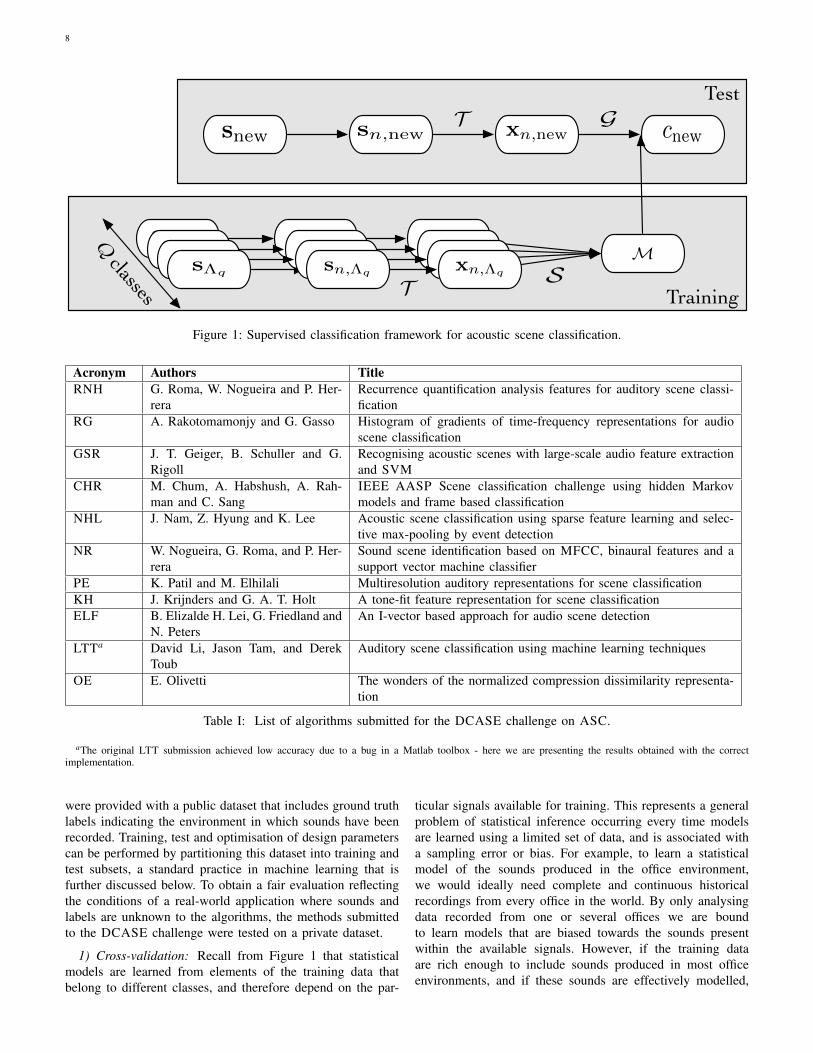
Figure 1: Supervised classification framework for acoustic scene classification.

Acronym Authors TitleRNH G. Roma, W. Nogueira and P. Her-

reraRecurrence quantification analysis features for auditory scene classi-fication

RG A. Rakotomamonjy and G. Gasso Histogram of gradients of time-frequency representations for audioscene classification

GSR J. T. Geiger, B. Schuller and G.Rigoll

Recognising acoustic scenes with large-scale audio feature extractionand SVM

CHR M. Chum, A. Habshush, A. Rah-man and C. Sang

IEEE AASP Scene classification challenge using hidden Markovmodels and frame based classification

NHL J. Nam, Z. Hyung and K. Lee Acoustic scene classification using sparse feature learning and selec-tive max-pooling by event detection

NR W. Nogueira, G. Roma, and P. Her-rera

Sound scene identification based on MFCC, binaural features and asupport vector machine classifier

PE K. Patil and M. Elhilali Multiresolution auditory representations for scene classificationKH J. Krijnders and G. A. T. Holt A tone-fit feature representation for scene classificationELF B. Elizalde H. Lei, G. Friedland and

N. PetersAn I-vector based approach for audio scene detection

LTTa David Li, Jason Tam, and DerekToub

Auditory scene classification using machine learning techniques

OE E. Olivetti The wonders of the normalized compression dissimilarity representa-tion

Table I: List of algorithms submitted for the DCASE challenge on ASC.

aThe original LTT submission achieved low accuracy due to a bug in a Matlab toolbox - here we are presenting the results obtained with the correctimplementation.

were provided with a public dataset that includes ground truthlabels indicating the environment in which sounds have beenrecorded. Training, test and optimisation of design parameterscan be performed by partitioning this dataset into training andtest subsets, a standard practice in machine learning that isfurther discussed below. To obtain a fair evaluation reflectingthe conditions of a real-world application where sounds andlabels are unknown to the algorithms, the methods submittedto the DCASE challenge were tested on a private dataset.

1) Cross-validation: Recall from Figure 1 that statisticalmodels are learned from elements of the training data thatbelong to different classes, and therefore depend on the par-

ticular signals available for training. This represents a generalproblem of statistical inference occurring every time modelsare learned using a limited set of data, and is associated witha sampling error or bias. For example, to learn a statisticalmodel of the sounds produced in the office environment,we would ideally need complete and continuous historicalrecordings from every office in the world. By only analysingdata recorded from one or several offices we are boundto learn models that are biased towards the sounds presentwithin the available signals. However, if the training dataare rich enough to include sounds produced in most officeenvironments, and if these sounds are effectively modelled,

9

Method Features Statistical model Decision criterionSawhney and Maes[42]

Filter bank None Nearest neighbour →majority vote

Clarkson et al. [12] MFCS HMM Maximum likelihoodEronen et al. [20] MFCCS, low-level descriptors, en-

ergy/frequency, LPCS → ICA, PCADiscriminative HMM Maximum likelihood

Aucouturier [2] MFCCS GMMS Nearest neighbourChu et al. [10] MFCCS, parametric (Gabor) GMMS Maximum likelihoodMalkin and Waibel[34]

MFCCS, low-level descriptors →PCA

Linear auto-encoder networks Maximum likelihood

Cauchi [8] NMF Maximum likelihoodBenetos [6] PLCA Maximum likelihoodHeittola et al. [27] Acoustic events Histogram Maximum likelihoodChaudhuri et al.[9]

Acoustic unit descriptors N-gram language models Maximum likelihood

DCASE SubmissionsBaseline MFCCS GMMS Maximum likelihoodRNH MFCCS RQA, moments → SVM -RG Local gradient histograms (learned on

time-frequency patches)Aggregation → SVM One versus one

Method Features Statistical model Decision criterionGSR MFCCS, energy/frequency, voicing Moments, percentiles, linear re-

gression coeff. → SVMMajority vote

CHR Energy/frequency SVM One versus all, major-ity vote

NHL Learned (MFCCS → SRBM) Selective max pooling → SVM One versus allNR MFCCS, energy/frequency, spatial →

Fisher feature selectionSVM Majority vote

PE filter bank → parametric (Gabor) →PCA

SVM One versus one,weighted majorityvote

KH Voicing Moments, percentiles → SVM -ELF MFCCS i-vector → PLDA Maximum likelihoodLTT MFCCS Ensemble of classification trees majority vote → tree-

baggerOE Size of compressed audio Compression distance -> ensemble

of classification trees- → random forest

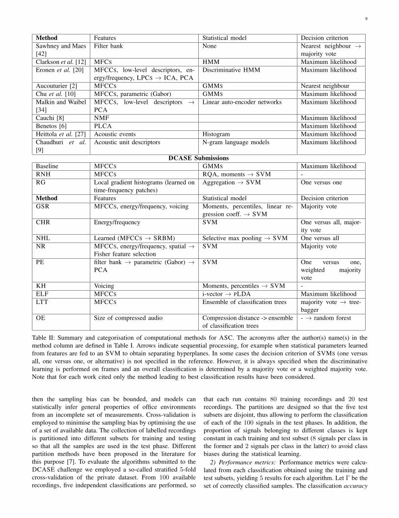
Table II: Summary and categorisation of computational methods for ASC. The acronyms after the author(s) name(s) in themethod column are defined in Table I. Arrows indicate sequential processing, for example when statistical parameters learnedfrom features are fed to an SVM to obtain separating hyperplanes. In some cases the decision criterion of SVMS (one versusall, one versus one, or alternative) is not specified in the reference. However, it is always specified when the discriminativelearning is performed on frames and an overall classification is determined by a majority vote or a weighted majority vote.Note that for each work cited only the method leading to best classification results have been considered.

then the sampling bias can be bounded, and models canstatistically infer general properties of office environmentsfrom an incomplete set of measurements. Cross-validation isemployed to minimise the sampling bias by optimising the useof a set of available data. The collection of labelled recordingsis partitioned into different subsets for training and testingso that all the samples are used in the test phase. Differentpartition methods have been proposed in the literature forthis purpose [7]. To evaluate the algorithms submitted to theDCASE challenge we employed a so-called stratified 5-foldcross-validation of the private dataset. From 100 availablerecordings, five independent classifications are performed, so

that each run contains 80 training recordings and 20 testrecordings. The partitions are designed so that the five testsubsets are disjoint, thus allowing to perform the classificationof each of the 100 signals in the test phases. In addition, theproportion of signals belonging to different classes is keptconstant in each training and test subset (8 signals per class inthe former and 2 signals per class in the latter) to avoid classbiases during the statistical learning.

2) Performance metrics: Performance metrics were calcu-lated from each classification obtained using the training andtest subsets, yielding 5 results for each algorithm. Let Γ be theset of correctly classified samples. The classification accuracy

10

is defined as the proportion of correctly classified soundsrelative to the total number of test samples. The confusionmatrix is a Q × Q matrix whose (i, j)-th element indicatesthe number of elements belonging to the i-th class that havebeen classified as belonging to the j-th class. In a problemwith Q = 10 different classes, chance classification has anaccuracy of 0.1 and a perfect classifier as an accuracy of 1.The confusion matrix of a perfect classifier is a diagonal matrixwhose (i, i)-th elements correspond to the number of samplesbelonging to the i-th class.

B. Results

Figure 2 depicts the results for the algorithms submitted tothe DCASE challenge (see Table I for the acronyms of themethods). The central dots are the percentage accuracies ofeach technique calculated by averaging the results obtainedfrom the 5 folds, and the bars are the relative confidenceintervals. These intervals are defined by assuming that theaccuracy value obtained from each fold is a realisation of aGaussian process whose expectation is the true value of theoverall accuracy (that is, the value that we would be able tomeasure if we evaluated an infinite number of folds). The totallength of each bar is the magnitude of a symmetric confidenceinterval computed as the product of the 95% quantile of astandard normal distribution q0.95

N (0,1) ≈ 3.92 and the standarderror of the accuracy (that is, the ratio between the standarddeviation of the accuracies of the folds and the square root ofthe number of folds σ/

√5). Under the Gaussian assumption,

confidence intervals are interpreted as covering with 95%probability the true value of the expectation of the accuracy.

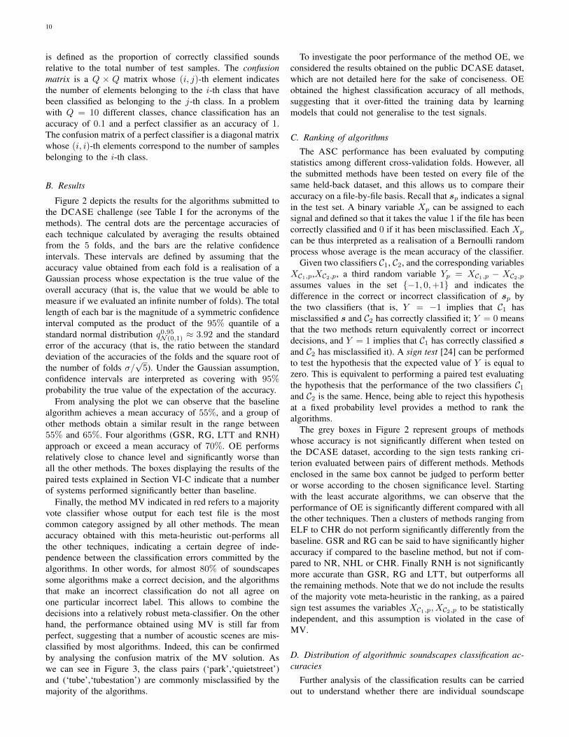
From analysing the plot we can observe that the baselinealgorithm achieves a mean accuracy of 55%, and a group ofother methods obtain a similar result in the range between55% and 65%. Four algorithms (GSR, RG, LTT and RNH)approach or exceed a mean accuracy of 70%. OE performsrelatively close to chance level and significantly worse thanall the other methods. The boxes displaying the results of thepaired tests explained in Section VI-C indicate that a numberof systems performed significantly better than baseline.

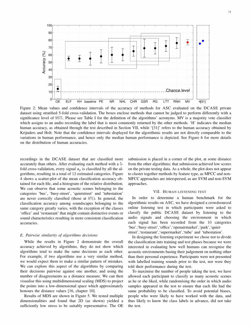
Finally, the method MV indicated in red refers to a majorityvote classifier whose output for each test file is the mostcommon category assigned by all other methods. The meanaccuracy obtained with this meta-heuristic out-performs allthe other techniques, indicating a certain degree of inde-pendence between the classification errors committed by thealgorithms. In other words, for almost 80% of soundscapessome algorithms make a correct decision, and the algorithmsthat make an incorrect classification do not all agree onone particular incorrect label. This allows to combine thedecisions into a relatively robust meta-classifier. On the otherhand, the performance obtained using MV is still far fromperfect, suggesting that a number of acoustic scenes are mis-classified by most algorithms. Indeed, this can be confirmedby analysing the confusion matrix of the MV solution. Aswe can see in Figure 3, the class pairs (‘park’,‘quietstreet’)and (‘tube’,‘tubestation’) are commonly misclassified by themajority of the algorithms.

To investigate the poor performance of the method OE, weconsidered the results obtained on the public DCASE dataset,which are not detailed here for the sake of conciseness. OEobtained the highest classification accuracy of all methods,suggesting that it over-fitted the training data by learningmodels that could not generalise to the test signals.

C. Ranking of algorithms

The ASC performance has been evaluated by computingstatistics among different cross-validation folds. However, allthe submitted methods have been tested on every file of thesame held-back dataset, and this allows us to compare theiraccuracy on a file-by-file basis. Recall that sp indicates a signalin the test set. A binary variable Xp can be assigned to eachsignal and defined so that it takes the value 1 if the file has beencorrectly classified and 0 if it has been misclassified. Each Xp

can be thus interpreted as a realisation of a Bernoulli randomprocess whose average is the mean accuracy of the classifier.

Given two classifiers C1, C2, and the corresponding variablesXC1,p,XC2,p, a third random variable Yp = XC1,p − XC2,passumes values in the set {−1, 0,+1} and indicates thedifference in the correct or incorrect classification of sp bythe two classifiers (that is, Y = −1 implies that C1 hasmisclassified s and C2 has correctly classified it; Y = 0 meansthat the two methods return equivalently correct or incorrectdecisions, and Y = 1 implies that C1 has correctly classified sand C2 has misclassified it). A sign test [24] can be performedto test the hypothesis that the expected value of Y is equal tozero. This is equivalent to performing a paired test evaluatingthe hypothesis that the performance of the two classifiers C1and C2 is the same. Hence, being able to reject this hypothesisat a fixed probability level provides a method to rank thealgorithms.

The grey boxes in Figure 2 represent groups of methodswhose accuracy is not significantly different when tested onthe DCASE dataset, according to the sign tests ranking cri-terion evaluated between pairs of different methods. Methodsenclosed in the same box cannot be judged to perform betteror worse according to the chosen significance level. Startingwith the least accurate algorithms, we can observe that theperformance of OE is significantly different compared with allthe other techniques. Then a clusters of methods ranging fromELF to CHR do not perform significantly differently from thebaseline. GSR and RG can be said to have significantly higheraccuracy if compared to the baseline method, but not if com-pared to NR, NHL or CHR. Finally RNH is not significantlymore accurate than GSR, RG and LTT, but outperforms allthe remaining methods. Note that we do not include the resultsof the majority vote meta-heuristic in the ranking, as a pairedsign test assumes the variables XC1,p, XC2,p to be statisticallyindependent, and this assumption is violated in the case ofMV.

D. Distribution of algorithmic soundscapes classification ac-curacies

Further analysis of the classification results can be carriedout to understand whether there are individual soundscape

11

OE ELF KH baseline PE NR NHL CHR GSR RG LTT RNH MV0

10

20

30

40

50

60

70

80

90

100

Chance level

Accura

cy (

%)

H[31]

Figure 2: Mean values and confidence intervals of the accuracy of methods for ASC evaluated on the DCASE privatedataset using stratified 5-fold cross-validation. The boxes enclose methods that cannot be judged to perform differently with asignificance level of 95%. Please see Table I for the definition of the algorithms’ acronyms. MV is a majority vote classifierwhich assigns to an audio recording the label that is most commonly returned by the other methods. ‘H’ indicates the medianhuman accuracy, as obtained through the test described in Section VII, while ‘[31]’ refers to the human accuracy obtained byKrijnders and Holt. Note that the confidence intervals displayed for the algorithmic results are not directly comparable to thevariations in human performance, and hence only the median human performance is depicted. See Figure 6 for more detailson the distribution of human accuracies.

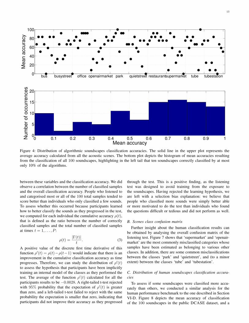
recordings in the DCASE dataset that are classified moreaccurately than others. After evaluating each method with a 5-fold cross-validation, every signal sp is classified by all the al-gorithms, resulting in a total of 12 estimated categories. Figure4 shows a scatter-plot of the mean classification accuracy ob-tained for each file, and a histogram of the relative distribution.We can observe that some acoustic scenes belonging to thecategories ‘bus’, ‘busy-street’, ‘quietstreet’ and ‘tubestation’are never correctly classified (those at 0%). In general, theclassification accuracy among soundscapes belonging to thesame category greatly varies, with the exception of the classes‘office’ and ‘restaurant’ that might contain distinctive events orsound characteristics resulting in more consistent classificationaccuracies.

E. Pairwise similarity of algorithms decisions

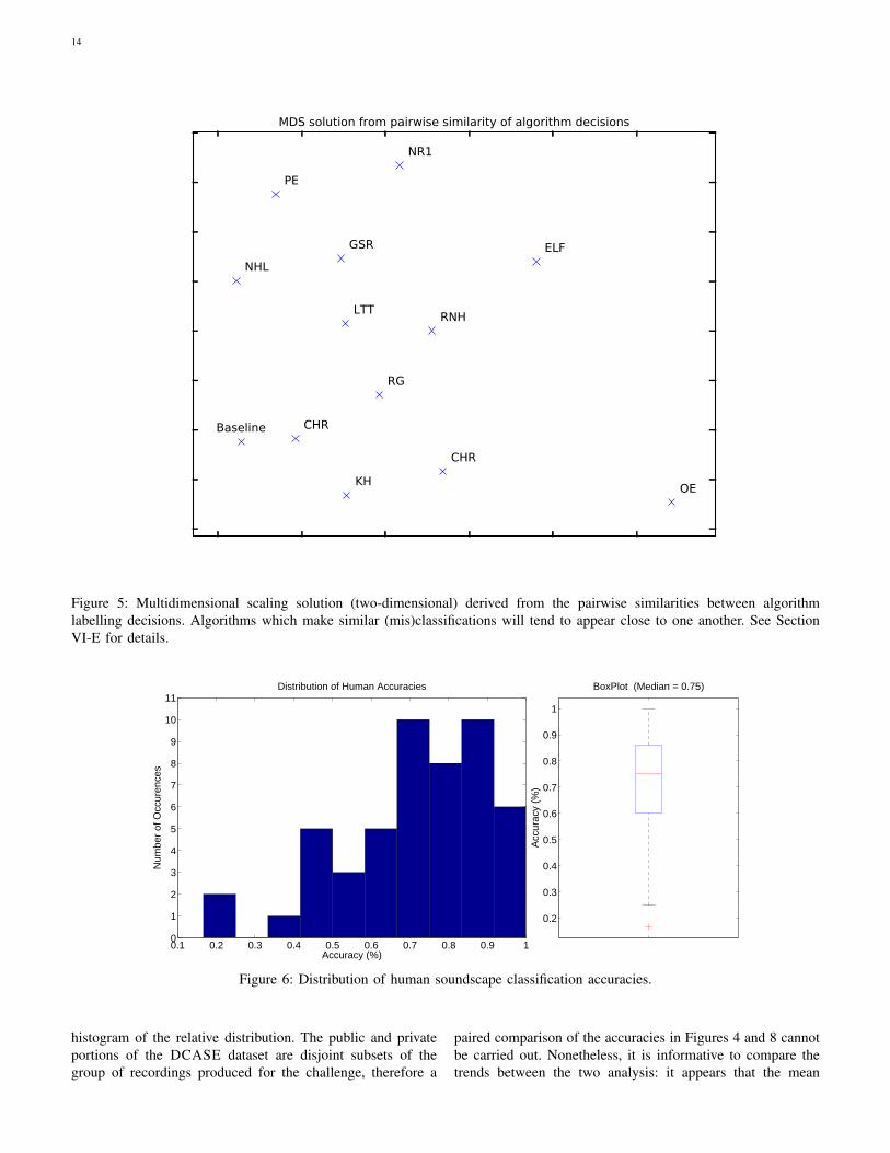
While the results in Figure 2 demonstrate the overallaccuracy achieved by algorithms, they do not show whichalgorithms tend to make the same decisions as each other.For example, if two algorithms use a very similar method,we would expect them to make a similar pattern of mistakes.We can explore this aspect of the algorithms by comparingtheir decisions pairwise against one another, and using thenumber of disagreements as a distance measure. We can thenvisualise this using multidimensional scaling (MDS) to projectthe points into a low-dimensional space which approximatelyhonours the distance values [16, chapter 10].

Results of MDS are shown in Figure 5. We tested multipledimensionalities and found that 2D (as shown) yielded asufficiently low stress to be suitably representative. The OE

submission is placed in a corner of the plot, at some distancefrom the other algorithms; that submission achieved low scoreson the private testing data. As a whole, the plot does not appearto cluster together methods by feature type, as MFCC and non-MFCC approaches are interspersed, as are SVM and non-SVMapproaches.

VII. HUMAN LISTENING TEST

In order to determine a human benchmark for thealgorithmic results on ASC, we have designed a crowdsourcedonline listening test in which participants were asked toclassify the public DCASE dataset by listening to theaudio signals and choosing the environment in whicheach signal has been recorded from the 10 categories‘bus’,‘busy-street’,‘office’,‘openairmarket’,‘park’,‘quiet-street’,‘restaurant’,‘supermarket’,‘tube’ and ‘tubestation’.

In designing the listening experiment we chose not to dividethe classification into training and test phases because we wereinterested in evaluating how well humans can recognise theacoustic environments basing their judgement on nothing otherthan their personal experience. Participants were not presentedwith labelled training sounds prior to the test, nor were theytold their performance during the test.

To maximise the number of people taking the test, we haveallowed each participant to classify as many acoustic scenesas he or she liked, while randomising the order in which audiosamples appeared in the test to ensure that each file had thesame probability to be classified. To avoid potential biases,people who were likely to have worked with the data, andthus likely to know the class labels in advance, did not takethe test.

12

bus

busy

stre

et

off

ice

openair

mark

et

park

quie

tstr

eet

rest

aura

nt

superm

ark

et

tube

tubest

ati

on

Estimate

bus

busystreet

office

openairmarket

park

quietstreet

restaurant

supermarket

tube

tubestation

Cate

gory

100

100

90 10

80 10 10

10 80 10

50 50

20 70 10

10 10 10 60 10

10 80 10

10 30 60

Figure 3: Confusion matrix of MV algorithmic classification results.

A. Human accuracy

A total of 50 participants took part in the test. Their mostcommon age was between 25 and 34 years old, while themost common listening device employed during the test was“high quality headphones”. Special care was taken to remove“test” cases or invalid attempts from the sample. This includedparticipants clearly labelled as “test” in the metadata, and par-ticipants who only attempted to label only 1− 2 soundscapes,and most of whom achieved scores as low as 0% that pointsto outliers with a clear lack of motivation. Figure 6 showsthat the mean accuracy among all participants was 72%, andthe distribution of accuracies reveals that most people scoredbetween 60% and 100%, with two outlier whose accuracywas as low as 20%. Since the distribution of accuracies isnot symmetric, we show a box plot summarising its statisticsinstead of reporting confidence intervals for the mean accuracy.The median value of the participants’ accuracy was 75%,the first and third quartiles are located at around 60% and

85%, while the 95% of values lie between around 45% and100%. Note that, although we decided to include the resultsfrom all the participants in the study who classified at leasta few soundscapes, the most extreme points (correspondingto individuals who obtained accuracies of about 25% and100% respectively) only include classifications performed onless than 10 acoustic scenes. Removing from the resultsparticipants who achieved about 25% accuracy would resultin a mean of 74% a lot closer to the median value. In a morecontrolled listening test, Krijnders and Holt [31] engaged 37participants, with each participant asked to listen to 50 publicDCASE soundscapes and select one of the 10 categories. Theparticipants were required to listen for the entire durationof the recordings, and use the same listening device. Theyobtained a mean accuracy of 79%, which is in the same areaas the results of our crowdsourced study (75%).

1) Cumulative accuracy: During the test, we asked theparticipants to indicate their age and the device they used tolisten to the audio signals, but we did not observe correlation

13

0

20

40

60

80

100

bus busystreet office openairmarket park quietstreet restaurantsupermarket tube tubestation

Me

an

accu

racy

0 0.1 0.2 0.3 0.4 0.5 0.6 0.7 0.8 0.9 10

5

10

15

20

Mean accuracy

Nu

mb

er

of

occu

rre

nce

s

Figure 4: Distribution of algorithmic soundscapes classification accuracies. The solid line in the upper plot represents theaverage accuracy calculated from all the acoustic scenes. The bottom plot depicts the histogram of mean accuracies resultingfrom the classification of all 100 soundscapes, highlighting in the left tail that ten soundscapes correctly classified by at mostonly 10% of the algorithms.

between these variables and the classification accuracy. We didobserve a correlation between the number of classified samplesand the overall classification accuracy. People who listened toand categorised most or all of the 100 total samples tended toscore better than individuals who only classified a few sounds.To assess whether this occurred because participants learnedhow to better classify the sounds as they progressed in the test,we computed for each individual the cumulative accuracy ρ(t),that is defined as the ratio between the number of correctlyclassified samples and the total number of classified samplesat times t = 1, . . . , P :

ρ(t) =|Γ(t)|t

. (3)

A positive value of the discrete first time derivative of thisfunction ρ′(t) = ρ(t)−ρ(t−1) would indicate that there is animprovement in the cumulative classification accuracy as timeprogresses. Therefore, we can study the distribution of ρ′(t)to assess the hypothesis that participants have been implicitlytraining an internal model of the classes as they performed thetest. The average of the function ρ′(t) calculated for all theparticipants results to be −0.0028. A right-tailed t-test rejectedwith 95% probability that the expectation of ρ′(t) is greaterthan zero, and a left-tailed t-test failed to reject with the sameprobability the expectation is smaller that zero, indicating thatparticipants did not improve their accuracy as they progressed

through the test. This is a positive finding, as the listeningtest was designed to avoid training from the exposure tothe soundscapes. Having rejected the learning hypothesis, weare left with a selection bias explanation: we believe thatpeople who classified more sounds were simply better ableor more motivated to do the test than individuals who foundthe questions difficult or tedious and did not perform as well.

B. Scenes class confusion matrix

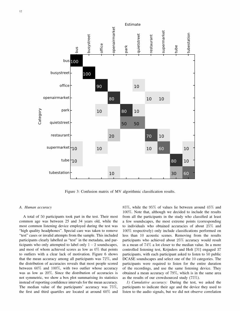
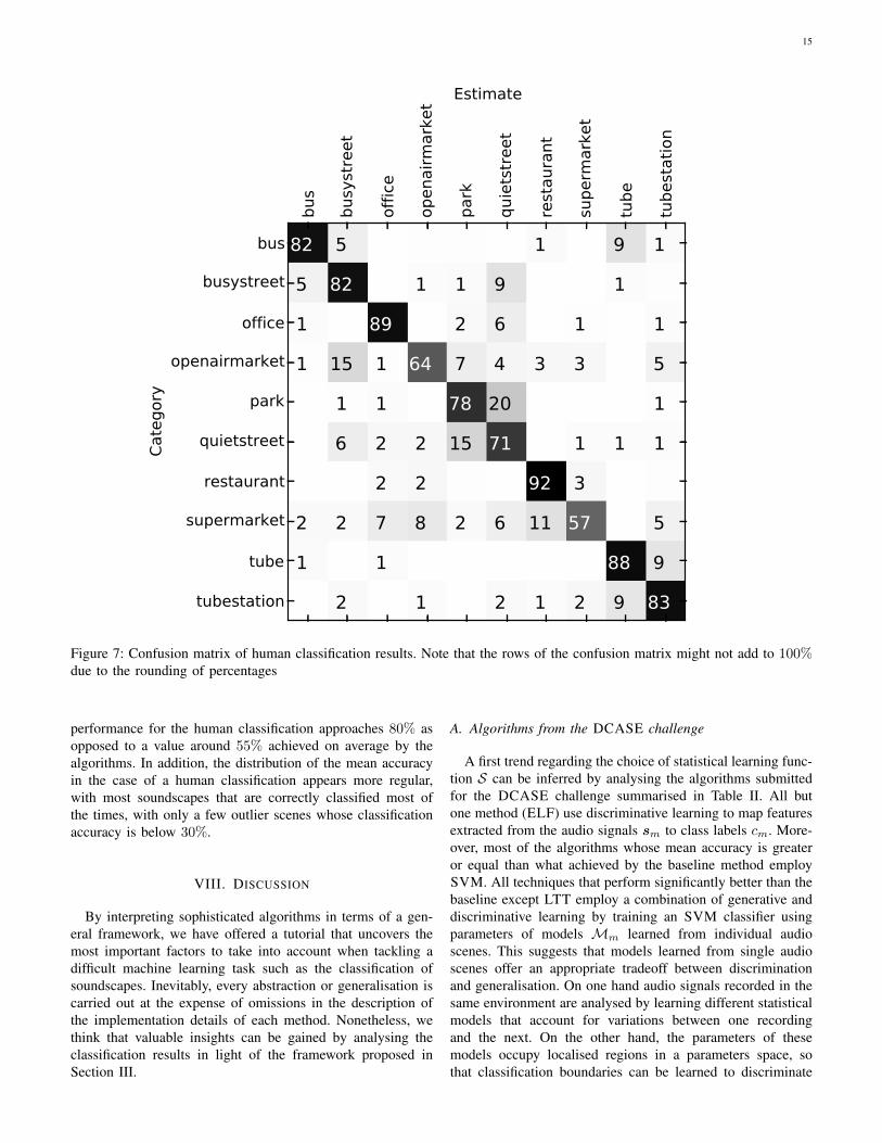
Further insight about the human classification results canbe obtained by analysing the overall confusion matrix of thelistening test. Figure 7 shows that ‘supermarket’ and ‘openair-market’ are the most commonly misclassified categories whosesamples have been estimated as belonging to various otherclasses. In addition, there are some common misclassificationsbetween the classes ‘park’ and ‘quietstreet’, and (to a minorextent) between the classes ‘tube’ and ‘tubestation’.

C. Distribution of human soundscapes classification accura-cies

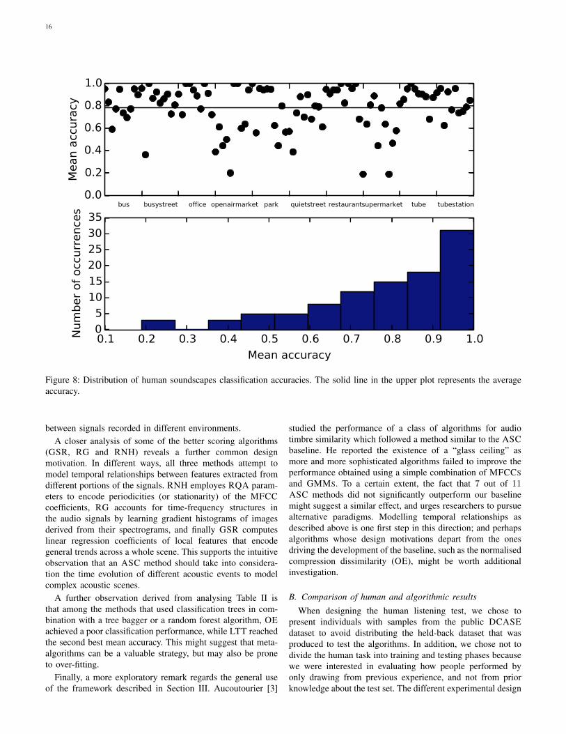
To assess if some soundscapes were classified more accu-rately than others, we conducted a similar analysis for thehuman performance benchmark to the one described in SectionVI-D. Figure 8 depicts the mean accuracy of classificationof the 100 soundscapes in the public DCASE dataset, and a

14

LTT

ELFGSR

PE

KH

NR1

RNH

NHL

OE

CHR

CHR

RG

Baseline

MDS solution from pairwise similarity of algorithm decisions

Figure 5: Multidimensional scaling solution (two-dimensional) derived from the pairwise similarities between algorithmlabelling decisions. Algorithms which make similar (mis)classifications will tend to appear close to one another. See SectionVI-E for details.

0.2

0.3

0.4

0.5

0.6

0.7

0.8

0.9

1

Acc

urac

y (%

)

BoxPlot (Median = 0.75)

0.1 0.2 0.3 0.4 0.5 0.6 0.7 0.8 0.9 10

1

2

3

4

5

6

7

8

9

10

11

Accuracy (%)

Num

ber

of O

ccur

ence

s

Distribution of Human Accuracies

Figure 6: Distribution of human soundscape classification accuracies.

histogram of the relative distribution. The public and privateportions of the DCASE dataset are disjoint subsets of thegroup of recordings produced for the challenge, therefore a

paired comparison of the accuracies in Figures 4 and 8 cannotbe carried out. Nonetheless, it is informative to compare thetrends between the two analysis: it appears that the mean

15

bus

busy

stre

et

off

ice

openair

mark

et

park

quie

tstr

eet

rest

aura

nt

superm

ark

et

tube

tubest

ati

on

Estimate

bus

busystreet

office

openairmarket

park

quietstreet

restaurant

supermarket

tube

tubestation

Cate

gory

82 5 1 9 1

5 82 1 1 9 1

1 89 2 6 1 1

1 15 1 64 7 4 3 3 5

1 1 78 20 1

6 2 2 15 71 1 1 1

2 2 92 3

2 2 7 8 2 6 11 57 5

1 1 88 9

2 1 2 1 2 9 83

Figure 7: Confusion matrix of human classification results. Note that the rows of the confusion matrix might not add to 100%due to the rounding of percentages

performance for the human classification approaches 80% asopposed to a value around 55% achieved on average by thealgorithms. In addition, the distribution of the mean accuracyin the case of a human classification appears more regular,with most soundscapes that are correctly classified most ofthe times, with only a few outlier scenes whose classificationaccuracy is below 30%.

VIII. DISCUSSION

By interpreting sophisticated algorithms in terms of a gen-eral framework, we have offered a tutorial that uncovers themost important factors to take into account when tackling adifficult machine learning task such as the classification ofsoundscapes. Inevitably, every abstraction or generalisation iscarried out at the expense of omissions in the description ofthe implementation details of each method. Nonetheless, wethink that valuable insights can be gained by analysing theclassification results in light of the framework proposed inSection III.

A. Algorithms from the DCASE challenge

A first trend regarding the choice of statistical learning func-tion S can be inferred by analysing the algorithms submittedfor the DCASE challenge summarised in Table II. All butone method (ELF) use discriminative learning to map featuresextracted from the audio signals sm to class labels cm. More-over, most of the algorithms whose mean accuracy is greateror equal than what achieved by the baseline method employSVM. All techniques that perform significantly better than thebaseline except LTT employ a combination of generative anddiscriminative learning by training an SVM classifier usingparameters of models Mm learned from individual audioscenes. This suggests that models learned from single audioscenes offer an appropriate tradeoff between discriminationand generalisation. On one hand audio signals recorded in thesame environment are analysed by learning different statisticalmodels that account for variations between one recordingand the next. On the other hand, the parameters of thesemodels occupy localised regions in a parameters space, sothat classification boundaries can be learned to discriminate

16

0.0

0.2

0.4

0.6

0.8

1.0M

ean a

ccura

cy

bus busystreet office openairmarket park quietstreet restaurantsupermarket tube tubestation

0.1 0.2 0.3 0.4 0.5 0.6 0.7 0.8 0.9 1.0

Mean accuracy

05

101520253035

Num

ber

of

occ

urr

ence

s

Figure 8: Distribution of human soundscapes classification accuracies. The solid line in the upper plot represents the averageaccuracy.

between signals recorded in different environments.A closer analysis of some of the better scoring algorithms

(GSR, RG and RNH) reveals a further common designmotivation. In different ways, all three methods attempt tomodel temporal relationships between features extracted fromdifferent portions of the signals. RNH employes RQA param-eters to encode periodicities (or stationarity) of the MFCCcoefficients, RG accounts for time-frequency structures inthe audio signals by learning gradient histograms of imagesderived from their spectrograms, and finally GSR computeslinear regression coefficients of local features that encodegeneral trends across a whole scene. This supports the intuitiveobservation that an ASC method should take into considera-tion the time evolution of different acoustic events to modelcomplex acoustic scenes.

A further observation derived from analysing Table II isthat among the methods that used classification trees in com-bination with a tree bagger or a random forest algorithm, OEachieved a poor classification performance, while LTT reachedthe second best mean accuracy. This might suggest that meta-algorithms can be a valuable strategy, but may also be proneto over-fitting.

Finally, a more exploratory remark regards the general useof the framework described in Section III. Aucoutourier [3]

studied the performance of a class of algorithms for audiotimbre similarity which followed a method similar to the ASCbaseline. He reported the existence of a “glass ceiling” asmore and more sophisticated algorithms failed to improve theperformance obtained using a simple combination of MFCCSand GMMS. To a certain extent, the fact that 7 out of 11ASC methods did not significantly outperform our baselinemight suggest a similar effect, and urges researchers to pursuealternative paradigms. Modelling temporal relationships asdescribed above is one first step in this direction; and perhapsalgorithms whose design motivations depart from the onesdriving the development of the baseline, such as the normalisedcompression dissimilarity (OE), might be worth additionalinvestigation.

B. Comparison of human and algorithmic results

When designing the human listening test, we chose topresent individuals with samples from the public DCASEdataset to avoid distributing the held-back dataset that wasproduced to test the algorithms. In addition, we chose not todivide the human task into training and testing phases becausewe were interested in evaluating how people performed byonly drawing from previous experience, and not from priorknowledge about the test set. The different experimental design

17

choices between human and algorithmic experiments do notallow us to perform a statistically rigorous comparison of theclassification performances. However, since the public andprivate DCASE datasets are two parts of a unique sessionof recordings realised with the same equipment and in thesame conditions, we still believe that qualitative comparisonsare likely to reflect what the results would have been hadwe employed a different design strategy that allowed a directcomparison. More importantly, we believe that qualitativeconclusions about how well algorithms can approach humancapabilities are more interesting than rigorous significancetests on how humans can perform according to protocols(like the 5-fold stratified cross-validation) that are a clearlyunnatural task.

Having specified the above disclaimer, several observationscan be derived from comparing algorithmic and human clas-sification results. Firstly, Figures 2 and 6 show that RNHachieves a mean accuracy in the classification of soundscapesof the private DCASE dataset that is similar to the medianaccuracy obtained by humans on the public DCASE dataset.This strongly suggests that the best performing algorithmdoes achieve similar accuracy compared to a median humanbenchmark.

Secondly, the analysis of misclassified acoustic scenes sum-marised in Figures 4 and 8 suggests that, by aggregating theresults from all the individuals who took part in the listeningtest, all the acoustic scenes are correctly classified by at leastsome individuals, while there are scenes that are misclassifiedby all algorithms. This observation echoes the problem of hubsencountered in music information retrieval, whereby certainsongs are always misclassified by algorithms [41]. Moreover,unlike for the algorithmic results, the distribution of humanerrors shows a gradual decrease in accuracy from the easiest tothe most challenging soundscapes. This observation indicatesthat, in the aggregate, the knowledge acquired by humansthrough experience still results in a better classification ofsoundscapes that might be considered to be ambiguous orlacking in highly distinctive elements.

Finally, the comparison of the confusion matrices pre-sented in Figure 3 and Figure 7 reveals that similar pairs ofclasses (‘park’ and ‘quietstreet’, or ‘tube’ and ‘tubestation’)are commonly misclassified by both humans and algorithms.Given what we found about the misclassification of singleacoustic scene, we do not infer from this observation thatthe algorithms are using techniques which emulate humanaudition. An alternative interpretation is rather that somegroups of classes are inherently more ambiguous than othersbecause they contain similar sound events. Even if both phys-ical and semantic boundaries between environments can beinherently ambiguous, for the purpose of training a classifierthe universe of soundscapes classes should be defined to bemutually exclusive and collectively exhaustive. In other words,it should include all the possible categories relevant to an ASCapplication, while ensuring that every category is as distinctas possible from all the others.

C. Further research

Several themes that have not been considered in this workmay be important depending on particular ASC applications,and are suggested here for further research.

1) Algorithm complexity: A first issue to be considered isthe complexity of algorithms designed to learn and classifyacoustic scenes. Given that mobile context-aware servicesare among the most relevant applications of ASC, particularemphasis should be placed in designing methods that can berun with the limited processing power available to smartphonesand tablets. The resources-intensive processing of trainingsignals to learn statistical models for classification can becarried out off-line, but the operators T and G still needto be applied to unlabelled signals and, depending on theapplication, might need to be simple enough to allow real-time classification results.

2) Continuous and user-assisted learning: Instead of as-suming a fixed set of categories as done in most publicationson ASC, a system might be designed to be progressivelytrained to recognise different environments. In this case, auser should record soundscape examples that are used totrain classification models (either on-line or off-line, using therecording device’s own computational resources or uploadingand processing the signals with remote cloud resources), andprogressively add new categories to the system’s memory ofsoundscapes. Users could also assist the training by confirmingor rejecting the category returned from querying each unla-belled signal, and thus refine the statistical models every time anew classification is performed. Such systems would inevitablyrequire more intervention by the user, but would likely result tobe more precise and relevant than totally automated systems.

3) Hierarchical classification: In this paper we have con-sidered a set of categories whose elements are assumed tobe mutually exclusive (that is, a soundscape can be classifiedas ‘bus’ or ‘park’ but not both). Alternatively, a hierarchicalclassification could be considered where certain categories aresubsets or supersets of others. For example, a system mightbe designed to classify between ‘outdoor’ and ‘indoor’ envi-ronments, and then to distinguish between different subsets ofthe two general classes. In this context, different costs couldbe associated with different types of misclassification errors:for example, algorithms could be trained to be very accuratein discriminating between ‘outdoor’ and ‘indoor’, and lessprecise in distinguishing between an outdoor ‘park’ and anoutdoor ‘busy-street’.

4) Acoustic scene detection: As a limit case of systemsthat employes non-uniform misclassification costs, algorithmsmight be designed to detect a particular environment and groupall the other irrelevant categories into an ‘others’ class. In thiscase, the system would essentially perform an acoustic scenedetection rather than classification.

5) Multi-modal learning: Another avenue of future re-search consists in fusing multi-modal information to improvethe classification accuracy of ASC systems. Video recordings,geo-location information, or temperature and humidity sensorsare all examples of data that can be used in conjunction withaudio signals to provide machines with context awareness.

18

6) Event detection and scene classification: The combina-tion of event detection algorithms and ASC which has alreadybeen object of research endeavours [27], [9] is likely to benefitfrom advances in both areas. Information regarding the eventsoccurring in an acoustic scene could be combined with moretraditional frame-based approaches to update the probabilityof categories as different events are detected. For example,while general spectral properties of a soundscape could beused to infer that a signal was likely to have been recorded ineither a ‘park’ or a ‘quiet street’, detecting the event ‘car horn’would help disambiguate between the two. Furthermore, thisBayesian strategy employed to update the posterior probabilityof different classes could be used to handle transitions betweendifferent environments.

7) Testing on different datasets: Finally, datasets that con-tain sounds from different acoustic environments have beenrecently released. They include the Diverse EnvironmentsMulti-channel Acoustic Noise Database (DEMAND) [48]and the Database of Annotated Real Environmental Sounds(DARES) [49].

IX. CONCLUSIONS

In this article we have offered a tutorial in ASC with aparticular emphasis on computational algorithms designed toperform this task automatically. By introducing a frameworkfor ASC, we have analysed and compared methods proposedin the literature in terms of their modular components. Wehave then presented the results of the DCASE challenge,which set the state-of-the-art in computational ASC, andcompared the results obtained by algorithms with a baselinemethod and a human benchmark. On one hand, many of thesubmitted techniques failed to significantly outperform thebaseline system, which was designed to be not optimisedfor this particular task. On the other hand, some methodssignificantly out-performed the baseline and approached anaccuracy comparable to the human benchmark. Nonetheless,a more careful analysis of the human and algorithmic resultshighlighted that some acoustic scenes were misclassified byall algorithms, while all soundscapes were correctly classifiedby at least some individuals. This suggests that there is stillscope for improvement before algorithms reach and surpassthe human ability to make sense of their environment basedon the sounds it produces.

X. ACKNOWLEDGMENTS

We would like to thank Dan Ellis, Toumas Virtanen, Jean-Julien Aucouturier, Mathieu Lagrange, Toni Heittola and theanonymous reviewers for having read and commented an earlydraft of this paper and on our submitted manuscript. Theirinsights and suggestions have substantially increased the valueof this work. We also would like to thank the IEEE AASPTechnical Committee for their support in the organisation ofthe DCASE challenge.

REFERENCES

[1] Extended abstracts, IEEE AASP Challenge on Detection andClassification of Acoustic Scenes and Events. Available athttp://c4dm.eecs.qmul.ac.uk/sceneseventschallenge/, 2013.

[2] J.-J. Aucouturier, B. Defreville, and F. Pachet. The bag-of-framesapproach to audio pattern recognition: a sufficient model for urbansoundscapes but not for polyphonic music. Journal of the AcousticalSociety of America, 112(2):881–891, 2007.

[3] J.-J. Aucouturier and F. Pachet. Improving timbre similarity: How highis the sky? Journal of negative results in speech and audio sciences,1(1), 2004.

[4] J. Ballas. Common factors in the identification of an assortment ofbrief everyday sounds. Journal of Experimental Psychology: HumanPerception and Performance, 19(2):250–267, 1993.

[5] J. Barker, E. Vincent, N. Ma, H. Christensen, and P. Green. The PASCALCHiME speech separation and recognition challenge. Computer Speech& Language, 27(3):621–633, 2012.

[6] E. Benetos, M. Lagrange, and S. Dixon. Characterisation of acousticscenes using a temporally-constrained shift-invariant model. In Pro-ceedings of the 15th International Conference on Digital Audio Effects(DAFx-12), 2012.

[7] C. Bishop. Pattern Recognition and Machine Learning. Springer, 2007.[8] B. Cauchi. Non-negative matrix factorization applied to auditory scene

classification. Master’s thesis, ATIAM (UPMC / IRCAM / TELECOMParisTech), 2011.

[9] S. Chaudhuri, M. Harvilla, and B. Raj. Unsupervised learning of acousticunit descriptors for audio content representation and classification. InProceedings of INTERSPEECH, pages 2265–2268, 2011.

[10] S. Chu, S. Narayanan, and C.-C. Jay Kuo. Environmental soundrecognition with time-frequency audio features. IEEE Trans. on Audio,Speech and Language Processing, 17(6):1142–1158, Aug. 2009.

[11] S. Chu, S. Narayanan, C.-C. Jay Kuo, and M. J. Matari. Where amI? Scene recognition for mobile robots using audio features. In IEEEInternational Conference on Multimedia and Expo, pages 885–888,2006.

[12] B. Clarkson, N. Sawhney, and A. Pentland. Auditory context awarenessvia wearable computing. In Proceedings Of The 1998 Workshop OnPerceptual User Interfaces (PUI’98), 1998.

[13] B. Defréville, P. Roy, C. Rosin, and F. Pachet. Automatic recognitionof urban sound sources. In Proceedings of the 120th Audio EngineeringSociety Convention, number 6827, 2006.

[14] N. Dehak, R. Dehak, P. Kenny, N. Brummer, P. Ouellet, and P. Du-mouchel. Support vector machines versus fast scornig in the low-dimensional total variability space for speaker verification. In Proceed-ings of INTERSPEECH, 2009.

[15] D. Dubois, C. Guastavino, and M. Raimbault. A cognitive approach tourban soundscapes: Using verbal data to access everyday life auditorycategories. Acta Acustica united with Acustica, 92:865–874, 2006.

[16] R. O. Duda, P. E. Hart, and D. G. Stork. Pattern Classification. Wiley-Interscience, 2nd edition, 2000.

[17] K. El-Maleh, A. Samouelian, and P. Kabal. Frame level noise classifica-tion in mobile environments. In Proceedings of the IEEE InternationalConference on Acoustics, Speech and Signal Processing (ICASSP),volume 1, pages 237–240, 1999.

[18] D. P. W. Ellis. Prediction-driven computational auditory scene analysis.PhD thesis, Massachusetts Institute of Technology, 1996.

[19] D. P. W. Ellis and K. Lee. Minimal-impact audio-based personalarchives. In Proceedings of the Workshop on Continuous Archiving andRecording of Personal Experiences, pages 39–47, 2004.

[20] A. J. Eronen, V. T. Peltonen, J. T. Tuomi, A. P. Klapuri, S. Fagerlund,T. Sorsa, G. Lorho, and J. Huopaniemi. Audio-based context recognition.IEEE Trans. on Audio, Speech and Language Processing, 14(1):321–329, Jan. 2006.

[21] A. J. Eronen, J. T. Tuomi, A. Klapuri, and S. Fagerlund. Audio-basedcontext awareness - acoustic modeling and perceptual evaluation. InProceedings of the IEEE International Conference on Acoustics, Speechand Signal Processing (ICASSP), volume 5, pages 529–532, 2003.

[22] P. Gaunard, C. G. Mubikangiey, C. Couvreur, and V. Fontaine. Auto-matic classification of environmental noise events by hidden markovmodels. In Proceedings of the IEEE International Conference onAcoustics, Speech and Signal Processing (ICASSP), volume 6, pages3609–3612, 1998.

[23] D. Giannoulis, D. Stowell, E. Benetos, M. Rossignol, M. Lagrange,and M. D. Plumbley. A database and challenge for acoustic sceneclassification and event detection. In Proceedings of the European SignalProcessing Conference (EUSIPCO), 2013.

19

[24] J. D. Gibbons and S. Chakraborti. Nonparametric Statistical Inference.Number 978-1420077612. Chapman and Hall, 5th edition, 2010.

[25] J. M. Grey and J. W. Gordon. Perceptual effects of spectral modificationson musical timbres. Journal of the Acoustical Society of America,63(5):1493–1500, 1978.

[26] P. Guyot, J. Pinquier, and R. André-Obrecht. Water sounds recognitionbased on physical models. In Proceedings of the IEEE InternationalConference on Acoustics, Speech and Signal Processing (ICASSP), pages793–797, 2013.

[27] T. Heittola, A. Mesaros, A. J. Eronen, and T. Virtanen. Audio contextrecognition using audio event histogram. In Proceedings of the EuropeanSignal Processing Conference (EUSIPCO), 2010.

[28] T. Heittola, A. Mesaros, A. J. Eronen, and T. Virtanen. Context-dependent sound event detection. EURASIP Journal on Audio, Speech,and Music Processing, 1:1–13, 2013.

[29] G. Hu and D. Wang. Auditory segmentation based on onset andoffset analysis. IEEE Transactions on Audio, Speech, and LanguageProcessing, 15(2):396–405, 2007.

[30] S. Ioffe. Probabilistic linear discriminant analysis. In Proceedings of the9th European Conference on Computer Vision (ECCV), pages 531–542,2006.

[31] J. Krijnders and G. A. t. Holt. Tone-fit and MFCC scene classificationcompared to human recognition. Personal Communication, Oct. 2013.

[32] C. Landone, J. Harrop, and J. Reiss. Enabling access to sound archivesthrough integration, enrichment and retrieval: the easaier project. InProceedings of the 8th International Conference on Music InformationRetrieval, Vienna, Austria, September 2007.

[33] L. Lu, H.-J. Zhang, and H. Jiang. Content analysis for audio classifi-cation and segmentation. IEEE Trans. on Audio, Speech and LanguageProcessing, 10(7):504–516, 2002.

[34] R. G. Malkin and A. Waibel. Classifying user environment for mobileapplications using linear autoencoding of ambient audio. In Proceedingsof the IEEE International Conference on Acoustics, Speech and SignalProcessing (ICASSP), volume 5, pages 509–512, 2005.

[35] S. McAdams. Recognition of sound sources and events. In S. McAdamsand E. Bigand, editors, Thinking in Sound: the Cognitive Psychology ofHuman Audition, pages 146—98. Oxford University Press, 1993.

[36] Music Information Retrieval Evaluation eXchange (MIREX).http://music-ir.org/mirexwiki/.

[37] V. T. Peltonen, A. J. Eronen, M. P. Parviainen, and A. P. Klapuri.Recognition of everyday auditory scenes: Potentials, latencies and cues.In Proceedings of the 110th Audio Engineering Society Convention,number 5404, 2001.

[38] V. T. Peltonen, J. T. Tuomi, A. Klapuri, J. Huopaniemi, and L. Sorsa.Computational auditory scene recognition. In Proceedings of the IEEEInternational Conference on Acoustics, Speech and Signal Processing(ICASSP), volume 2, pages 1941–1944, 2002.

[39] L. Rabiner and B.-H. Juang. Fundamentals of Speech Recognition.Number ISBN: 0-13-285826-6. Prentice-Hall, 1993.

[40] R. Radhakrishnan, A. Divakaran, and P. Smaragdis. Audio analysisfor surveillance applications. In Proceedings of the IEEE Workshop onApplications of Signal Processing to Audio and Acoustics (WASPAA),pages 158–161, 2005.

[41] M. Radovanovic, A. Nanopoulos, and M. Ivanovic. Hubs in space:Popular nearest neighbors in high-dimensional data. Journal of MachineLearning Research, 11:2487–2531, 2010.

[42] N. Sawhney and P. Maes. Situational awareness from environmentalsounds. Technical report, Massachussets Institute of Technology, 1997.

[43] M. Schafer. The tuning of the world. Random House, Rochester VT,1977.

[44] R. E. Schapire. The boosting approach to machine learning an overview,volume 171 of Lecture notes in statistics, pages 149–172. Springer,2003.

[45] B. Schilit, N. Adams, and R. Want. Context-aware computing applica-tions. In Proceedings of the Workshop on Mobile Computing Systemsand Applications, pages 85–90, 1994.

[46] Signal separation evaluation campaign (SiSEC).http://sisec.wiki.irisa.fr/tiki-index.php, 2013.

[47] J. Tardieu, P. Susini, F. Poisson, P. Lazareff, and S. McAdams. Percep-tual study of soundscapes in train stations. Applied Acoustics, 69:1224–1239, 2008.

[48] J. Thiemann, N. Ito, and E. Vincent. The Diverse EnvironmentsMulti-channel Acoustic Noise Database (DEMAND): A database ofmultichannel environmental noise recordings. In 21st InternationalCongress on Acoustics, Montreal, Canada, June 2013. Acoustical Societyof America.

[49] M. van Grootel, T. Andringa, and J. Krijnders. DARES-G1: Database ofannotated real-world everyday sounds. In Proceedings of the NAG/DAGAInternational Conference on Acoustics, 2009.

[50] P. Vandewalle, J. Kovacevic, and M. Vetterli. Reproducible researchin signal processing. IEEE Signal Processing Magazine, 26(3):37–47,2009.

[51] D. Wang and G. J. Brown. Computational Auditory Scene Analysis:Principles, Algorithms, and Applications. IEEE Press, 2006.

[52] Y. Xu, W. J. Li, and K. K. Lee. Intelligent Wearable Interfaces. ISBN978-0-470-17927-7. Wiley and Sons, 2008.

[53] T. Zhang and C.-C. Jay Kuo. Audio content analysis for onlineaudiovisual data segmantation and classification. IEEE Trans. on Audio,Speech and Language Processing, 9(4):441–457, 2001.

APPENDIX

A. MFCCs

Mel-frequency cepstral coefficients have been introduced inSection II-A and have been widely used as a feature for audioanalysis. Let sn ∈ RD be a signal frame and |sn| the absolutevalue of its Fourier transform. The coefficients correspondingto linearly-spaced frequency bins are mapped onto R Melfrequency bands to approximate the human perception ofpitches (which can be approximately described as logarithmic,meaning that we are capable of a much better resolutionat low frequencies than at high frequencies), resulting inL ≤ D coefficients. The magnitude of the Mel coefficientsis converted to a logarithmic scale, and the resulting vector isprocessed using a discrete cosine transform (DCT). Finally,the K ≤ R first coefficients are selected and constitute thevector of features xn = T (sn). This last step essentiallymeasures the frequency content of the log-magnitude of thespectrum of a signal, and therefore captures general propertiesof the spectral envelope. For example, periodic sounds whichexhibit spectral peaks at multiples of a fundamental frequencyare highly correlated with one or several cosine bases, en-coding this information in the value of the correspondingMFCC coefficients. The set of parameters θ = {D,R,K}includes frames dimension, number of Mel bands and numberof DCT coefficients which need to be defined when computingthe MFCCS. These parameters determine the dimensionalityreduction introduced by the features extraction operator, andtheir choice is governed by the tradeoff between generalisationand discrimination that has been mentioned in Section III.

1) Statistical normalization: To classify features extractedfrom signals belonging to different categories, it is importantto evaluate relative differences between the values of featurevectors belonging to different classes, rather than differencesbetween different coefficients within feature vectors extractedfrom the same signal. For this reason, during the trainingphase of the ASC classification algorithm, statistical normali-sation is performed as a standard feature processing aimed atavoiding offsets or scaling variations of any of the coefficientswithin feature vectors. This is accomplished by subtractingthe global mean (computed from features extracted from thewhole dataset) from each vector xn,m, and by dividing eachcoefficient by the their global standard deviation. After thefeature vectors have been normalised, the average and standarddeviation of the coefficients xn,m,k are 0 and 1 respectively.

20

B. GMMs

Gaussian mixture models (GMMS) have been introducedin Section II-C, and are used to infer global statistical prop-erties of the features from local features vectors, which areinterpreted as realisations of a generative stochastic process.Let N (µ,Σ) be a multivariate normal distribution with meanµ ∈ RK and covariance matrix Σ ∈ RK×K , and recallthat the notation xn,Λq identifies features vectors extractedfrom training signals that belong to the q-th category. Thenevery such vector is modelled as generated by the followingdistribution:

xn,Λq∼

I∏i=1

wiN (µi,Σi) (4)

where I is a fixed number of components, and wi is a latentvariable expressing the probability that a particular observationis generated from the i-th component.

The operator S takes the collection of features xn,Λqand

learns a global model for the q-th classMq = {wi,µi,Σi}Ii=1

by estimating the parameters of the Gaussian mixture distri-bution in Equation (4), which can be accomplished throughan expectation-maximisation (EM) algorithm [7]. The onlyparameter to be set in this case is the number of Gaussiancomponents I which rules a tradeoff between model accuracyand over-fitting. Indeed SI must include a sufficient numberof components to account for the fact that different eventswithin a soundscape generate sounds with different spectralproperties. However, as the number of components becomestoo large, the model tends to fit spurious random variations inthe training data, hindering the generalisation capabilities ofthe algorithm when confronted with an unlabelled sound.

C. Maximum likelihood criterion

Once the GMMS Mq have been learned from the trainingdata, features can be extracted from an unlabelled soundby applying the operator T . The new sequence of featuresxn,new is statistically normalised using the same mean andstandard deviation values obtained from the training signals,and a likelihood measure G is employed to evaluate whichclass is statistically most likely to generate the observedfeatures, hence determining the sound classification. A set ofcoefficients gq is computed by evaluating the log-likelihood ofthe observed data given the model:

gq = p(xn,new|Mq) ∝I∑

i=1

wi(xn,new − µi)TΣi(xn,new−µi)

(5)and a category is picked based on the most likely modelc?new = arg min

qgq .

Note that the baseline system described in this section isan example of a bag-of-frames technique where the orderingof the sequence of features is irrelevant. Indeed, any randompermutation of the sequences xn,Λq

does not affect the com-putation of the GMM parameters, and thus the classificationof unlabelled signals.