Embed Size (px)
Citation preview
ARTICLE IN PRESS
Journal of the Mechanics and Physics of Solids
55 (2007) 91–131
0022-5096/$ -
doi:10.1016/j
�CorrespoE-mail ad
1Present ad
www.elsevier.com/locate/jmps
Activation energy based extreme value statisticsand size effect in brittle and quasibrittle fracture
Zdenek P. Bazanta,�, Sze-Dai Pangb,1
aCivil Engineering and Materials Science, Northwestern University, 2145 Sheridan Road, CEE,
Evanston, IL 60208, USAbNorthwestern University, IL 60208, USA
Received 18 November 2005; accepted 31 May 2006
Abstract
Because the uncertainty in current empirical safety factors for structural strength is far larger than
the relative errors of structural analysis, improvements in statistics offer great promise. One
improvement, proposed here, is that, for quasibrittle structures of positive geometry, the
understrength factors for structural safety cannot be constant but must be increased with structures
size. The statistics of safety factors has so far been generally regarded as independent of mechanics,
but further progress requires the cumulative distribution function (cdf) to be derived from the
mechanics and physics of failure. To predict failure loads of extremely low probability (such as 10�6
to 10�7) on which structural design must be based, the cdf of strength of quasibrittle structures of
positive geometry is modelled as a chain (or series coupling) of representative volume elements
(RVE), each of which is statistically represented by a hierarchical model consisting of bundles (or
parallel couplings) of only two long sub-chains, each of them consisting of sub-bundles of two or
three long sub-sub-chains of sub-sub-bundles, etc., until the nano-scale of atomic lattice is reached.
Based on Maxwell–Boltzmann distribution of thermal energies of atoms, the cdf of strength of a
nano-scale connection is deduced from the stress dependence of the interatomic activation energy
barriers, and is expressed as a function of absolute temperature T and stress-duration t (or loading
rate 1=t). A salient property of this cdf is a power-law tail of exponent 1. It is shown how the
exponent and the length of the power-law tail of cdf of strength is changed by series couplings in
chains and by parallel couplings in bundles consisting of elements with either elastic–brittle or
elastic–plastic behaviors, bracketing the softening behavior which is more realistic, albeit more
difficult to analyze. The power-law tail exponent, which is 1 on the atomistic scale, is raised by the
see front matter r 2006 Published by Elsevier Ltd.
.jmps.2006.05.007
nding author. Tel.: +1847 491 4025; fax: +1 847 491 4011.
dress: [email protected] (Z.P. Bazant).
dress: Department of Civil Engineering, National University of Singapore, Singapore.
ARTICLE IN PRESSZ.P. Bazant, S.-D. Pang / J. Mech. Phys. Solids 55 (2007) 91–13192
hierarchical statistical model to an exponent of m ¼ 10 to 50, representing the Weibull modulus on
the structural scale. Its physical meaning is the minimum number of cuts needed to separate the
hierarchical model into two separate parts, which should be equal to the number of dominant cracks
needed to break the RVE. Thus, the model indicates the Weibull modulus to be governed by the
packing of inhomogeneities within an RVE. On the RVE scale, the model yields a broad core of
Gaussian cdf (i.e., error function), onto which a short power-law tail of exponent m is grafted at the
failure probability of about 0.0001–0.01. The model predicts how the grafting point moves to higher
failure probabilities as structure size increases, and also how the grafted cdf depends on T and t. Themodel provides a physical proof that, on a large enough scale (equivalent to at least 500 RVEs),
quasibrittle structures must follow Weibull distribution with a zero threshold. The experimental
histograms with kinks, which have so far been believed to require the use of a finite threshold, are
shown to be fitted much better by the present chain-of-RVEs model. For not too small structures, the
model is shown to be essentially a discrete equivalent of the previously developed nonlocal Weibull
theory, and to match the Type 1 size effect law previously obtained from this theory by asymptotic
matching. The mean stochastic response must agree with the cohesive crack model, crack band model
and nonlocal damage models. The chain-of-RVEs model can be verified and calibrated from the
mean size effect curve, as well as from the kink locations on experimental strength histograms for
sufficiently different specimen sizes.
r 2006 Published by Elsevier Ltd.
Keywords: Random strength; Failure probability; Maxwell–Boltzmann statistics; Safety factors; Nonlocal damage
1. Nature of problem
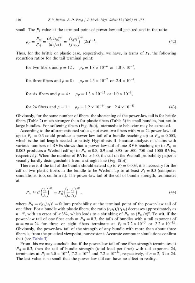
The type of probability distribution function (pdf) of structural strength has so far beenstudied separately from the mechanics of structural failure, as if these were independentproblems. For quasibrittle structures, however, such a separation is unjustified because thetype of pdf depends on structure size and geometry, and does so in a way that can bedetermined only by cohesive fracture or damage analysis. Structural safety dictates that thedesign must be based on extremely small failure probability, about 10�6 to 10�7 (Duckett,2005; Melchers, 1987; NKB, 1978).Since part of the uncertainty stems from the randomness of load, which is in structural
engineering taken into account by the load factors (Ellingwood et al., 1982; CIRIA, 1977),the knowledge of the far-left tail of pdf of strength need not extend that far. Based onintegrating the product of load and strength distributions (Freudenthal et al., 1966; Haldarand Mahadevan, 2000), joint probability computations show that the probability cut-offup to which the pdf tail must be known need not be as small as 10�6–10�7, but must still beonly about one order of magnitude larger, i.e., about 10�5–10�6 (Bazant, 2004a), providedthat, as usual, the load and resistance factors do not differ by more than about 3: 1 (thisrequirement is more stringent if the structural strength distribution has a Weibull, ratherthan Gaussian, tail).In the far-left tail, the pdf type makes a huge difference. For example, the difference of
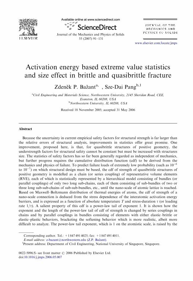
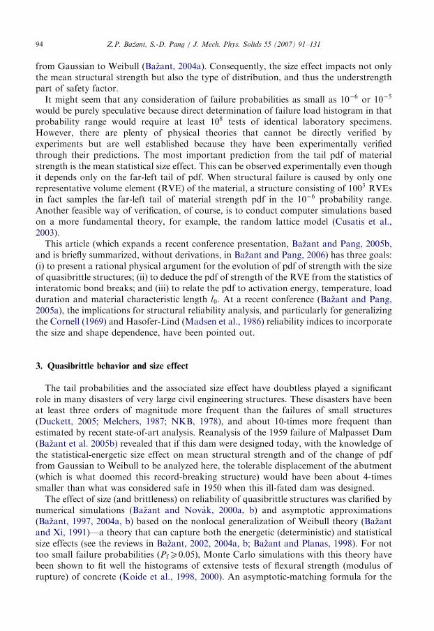
load with failure probability 10�6 from the mean failure load will almost double when thepdf changes from Gaussian to Weibull (with the same mean and same coefficient ofvariation (CoV); see Fig. 1).The importance of the problem is clear from the large values of safety factors. Defined as
the ratio of mean load capacity to the maximum service load, they are about 2 in the case
ARTICLE IN PRESS
log(xf /�)
xf /�
log(TW)
10-3
10-6
Pf
0
1
chosenPf = 10-6
Gaussian
Weibull
Weibull Gaussian
Pf
Means = 1 ω m = 24
TW
TG
log(TG)= 0.052
(a) (b)
Fig. 1. Large difference between points of failure probability 10�6 for Gaussian and Weibull distributions with
mean 1 and CoV ¼ 5:2% in (a) linear scale; (b) log scale.
Z.P. Bazant, S.-D. Pang / J. Mech. Phys. Solids 55 (2007) 91–131 93
of steel structures, or aeronautical and naval structures, while in the case of brittle failures(e.g., shear failures) of normal size concrete structures they are about 4 for design codeformulas and about 3 for finite element simulations (Bazant and Yu, 2006). Consequently,improvements in the stochastic fracture mechanics underlying the safety factors have thepotential of bringing about much greater benefits than improvements in the methods ofdeterministic structural analysis. It makes no sense at all to strive for a 5% to 10%accuracy improvement by more sophisticated computer simulations or analytical solutionsand then scale down the resulting load capacity by an empirical safety factor of 2 to 4which easily could have an error over 50%.
2. Background and objectives
While the mean statistical size effect in failures at macrocrack initiation is by nowunderstood quite well (e.g., Bazant and Planas, 1998, Chapter 12), and its combinationwith the deterministic size effect has recently also been clarified (Bazant and Xi, 1991;Bazant and Novak, 2000a, b, 2001; Bazant, 2004a, b; Carmeliet, 1994; Carmeliet andHens, 1994; Gutierez, 1999; Breysse, 1990; Frantziskonis, 1998), little is known about thetype of pdf to be assumed once the mean structural response has been calculated. What isclear is that the strength of brittle structures made, e.g., of fine-grained ceramics andfatigue-embrittled steel, must follow the Weibull distribution—by virtue of the weakest-link (or series coupling) model (because one small material element will trigger failure), andthat (except in the far-out tails) the strength of ductile (or plastic) structures must followthe Gaussian distribution—by virtue of the central limit theorem (CLT) of the theory ofprobability (because the limit load is a sum of contributions from all the plasticizedmaterial elements along the failure surface, as in parallel coupling).
Statistical models with parallel and series couplings have been extensively analyzed, e.g.,by Phoenix (1978, 1983), Phoenix and Smith (1983), McCartney and Smith (1983),McMeeking and Hbaieb (1999), Phoenix et al. (1997), Phoenix and Beyerlein (2000),Harlow and Phoenix (1978a, b), Harlow et al. (1983), Rao et al. (1999), Mahesh et al.(2002), Smith (1982) and Smith and Phoenix (1981). However, what seems to have beenunappreciated and has been brought to light only recently (Bazant, 2004a, b), on the basisof nonlocal Weibull theory (Bazant and Xi, 1991), is that the pdf of strength of aquasibrittle structure must gradually change with increasing size and shape (or brittleness)
ARTICLE IN PRESSZ.P. Bazant, S.-D. Pang / J. Mech. Phys. Solids 55 (2007) 91–13194
from Gaussian to Weibull (Bazant, 2004a). Consequently, the size effect impacts not onlythe mean structural strength but also the type of distribution, and thus the understrengthpart of safety factor.It might seem that any consideration of failure probabilities as small as 10�6 or 10�5
would be purely speculative because direct determination of failure load histogram in thatprobability range would require at least 108 tests of identical laboratory specimens.However, there are plenty of physical theories that cannot be directly verified byexperiments but are well established because they have been experimentally verifiedthrough their predictions. The most important prediction from the tail pdf of materialstrength is the mean statistical size effect. This can be observed experimentally even thoughit depends only on the far-left tail of pdf. When structural failure is caused by only onerepresentative volume element (RVE) of the material, a structure consisting of 1003 RVEsin fact samples the far-left tail of material strength pdf in the 10�6 probability range.Another feasible way of verification, of course, is to conduct computer simulations basedon a more fundamental theory, for example, the random lattice model (Cusatis et al.,2003).This article (which expands a recent conference presentation, Bazant and Pang, 2005b,
and is briefly summarized, without derivations, in Bazant and Pang, 2006) has three goals:(i) to present a rational physical argument for the evolution of pdf of strength with the sizeof quasibrittle structures; (ii) to deduce the pdf of strength of the RVE from the statistics ofinteratomic bond breaks; and (iii) to relate the pdf to activation energy, temperature, loadduration and material characteristic length l0. At a recent conference (Bazant and Pang,2005a), the implications for structural reliability analysis, and particularly for generalizingthe Cornell (1969) and Hasofer-Lind (Madsen et al., 1986) reliability indices to incorporatethe size and shape dependence, have been pointed out.
3. Quasibrittle behavior and size effect
The tail probabilities and the associated size effect have doubtless played a significantrole in many disasters of very large civil engineering structures. These disasters have beenat least three orders of magnitude more frequent than the failures of small structures(Duckett, 2005; Melchers, 1987; NKB, 1978), and about 10-times more frequent thanestimated by recent state-of-art analysis. Reanalysis of the 1959 failure of Malpasset Dam(Bazant et al. 2005b) revealed that if this dam were designed today, with the knowledge ofthe statistical-energetic size effect on mean structural strength and of the change of pdffrom Gaussian to Weibull to be analyzed here, the tolerable displacement of the abutment(which is what doomed this record-breaking structure) would have been about 4-timessmaller than what was considered safe in 1950 when this ill-fated dam was designed.The effect of size (and brittleness) on reliability of quasibrittle structures was clarified by
numerical simulations (Bazant and Novak, 2000a, b) and asymptotic approximations(Bazant, 1997, 2004a, b) based on the nonlocal generalization of Weibull theory (Bazantand Xi, 1991)—a theory that can capture both the energetic (deterministic) and statisticalsize effects (see the reviews in Bazant, 2002, 2004a, b; Bazant and Planas, 1998). For nottoo small failure probabilities ðPfX0:05Þ, Monte Carlo simulations with this theory havebeen shown to fit well the histograms of extensive tests of flexural strength (modulus ofrupture) of concrete (Koide et al., 1998, 2000). An asymptotic-matching formula for the
ARTICLE IN PRESSZ.P. Bazant, S.-D. Pang / J. Mech. Phys. Solids 55 (2007) 91–131 95
combined statistical-energetic size effect was shown to match well Jackson’s (1992) flexuralstrength tests of laminates at NASA.
Quasibrittle structures, consisting of quasibrittle materials, are those in which thefracture process zone (FPZ) is not negligible compared to the cross section dimension D
(and may even encompass the entire cross section). Depending on the scale of observationor application, quasibrittle materials include concrete, fiber composites, toughenedceramics, rigid foams, nanocomposites, sea ice, consolidated snow, rocks, mortar,masonry, fiber-reinforced concretes, stiff clays, silts, grouted soils, cemented sands, wood,paper, particle board, filled elastomers, various refractories, coal, dental cements, bone,cartilage, biological shells, cast iron, grafoil, and modern tough alloys. In these materials,the FPZ undergoes softening damage, such as microcracking, which occupies almost theentire nonlinear zone. By contrast, in ductile fracture of metals, the FPZ is essentially apoint within a nonnegligible (but still small) nonlinear zone undergoing plastic yieldingrather than damage.
The width of FPZ is typically about the triple of the dominant inhomogeneity size. Itslength can vary enormously; it is typically about 50 cm in normal concretes; 5 cm in high-strength concretes; 10–100mm in fine-grained ceramics; 10 nm in a silicon wafer; 100m in amountain mass intersected by rock joints; 1–10m in an Arctic sea ice floe; and about 50 kmin the ice cover of Arctic Ocean (consisting of thick floes a few km in size, connected bythin ice). If the cross section dimension (size) of structures is far larger than the FPZ size, aquasibrittle material becomes perfectly brittle, i.e., follows linear elastic fracture mechanics(LEFM). Thus, concrete is quasibrittle on the scale of normal beams and columns, butperfectly brittle on the scale of a large dam. Arctic Ocean cover, fine-grained ceramic ornanocomposite are quasibrittle on the scales of 10 km, 0.1mm or 0:1mm, but brittle on thescales of 1000 km, 1 cm or 10mm, respectively.
The FPZ width may be regarded as the size of the RVE of the material. The RVEdefinition cannot be the same as in the homogenization theory of elastic structures. TheRVE is here defined as the smallest material element whose failure causes the failure of thewhole structure (of positive geometry). From experience with microstructural simulationand testing, the size of RVE is roughly the triple of maximum inhomogeneity size (e.g., themaximum aggregate size in concrete or grain size in a ceramic).
According to the deterministic theories of elasticity and plasticity, geometrically similarstructures exhibit no size effect, i.e., their nominal strength, defined as
sN ¼ Pmax=bD (1)
is independent of characteristic structure size D (Pmax ¼ maximum load of the structure orparameter of load system; b ¼ structure thickness in the third dimension). The size effect isdefined as the dependence of sN on D. Structures whose material failure criterion isdeterministic and involves only the stress and strain tensors exhibit no size effect. Theclassical cause of size effect, proposed by Mariotte around 1650 and mathematicallydescribed by Weibull (1939), is the randomness of strength of a brittle material.Quasibrittle structures, whose material failure criterion involves a material characteristiclength l0 (implied by the material fracture energy or the crack softening curve), exhibit, inaddition, the energetic size effect (Bazant, 1984, 2002). This size effect is caused by energyrelease due to stress redistribution engendered by a large FPZ (or by stable growth of largecrack before reaching the maximum load).
ARTICLE IN PRESSZ.P. Bazant, S.-D. Pang / J. Mech. Phys. Solids 55 (2007) 91–13196
Two basic types of energetic size effect must be distinguished. The Type 1 size effect, theonly one studied here, occurs in positive geometry structures failing at macrocrackinitiation (positive geometry means that the stress intensity factor at constant loadincreases with the crack length). Type 2 occurs in structures containing a large notch or alarge stress-free (fatigued) crack formed prior to maximum load (there also exists a Type 3size effect, but it is very similar to Type 2); Bazant, 2002. For Type 2, material randomnessaffects significantly only the scatter of sN but not its mean (Bazant and Xi, 1991), while forType 1 it affects both, and so is more important. Type 1 is typical of flexural failures, inwhich the RVE size coincides with the thickness of the boundary layer of cracking. Thislayer causes stress redistribution and energy release before the maximum load is reached.This, in turn, engenders the Type 1 energetic size effect which dwarfs the statisticalWeibull-type size effect when the structure is small. A statistical size effect on mean sN issignificant only for Type 1.
4. Hypotheses of analysis
Hypothesis I. The failure of interatomic bonds is governed by the Maxwell–Boltzmanndistribution of thermal energies of atoms and the stress dependence of the activationenergy barriers of the interatomic potential.Hypothesis II. Quasibrittle structures (of positive geometry) that are at least 1000-
times larger than the material inhomogeneities, as well as laboratory specimens ofsufficiently fine-grained brittle materials, exhibit random strength that follows the Weibulldistribution.Hypothesis III. The cumulative distribution function (cdf) of strength of an RVE of
brittle or quasibrittle material may be described as Gaussian (or normal) except in the far-left power-law tail that reaches up to the failure probability of about 0.0001–0.01 (thishypothesis is justified, e.g., by Weibull’s tests of strength histograms of mortar discussedafter Eq. (69)).
5. Fundamental questions to answer
In the weakest-link statistical theory of strength, there remain four unansweredfundamental questions:
(1)
What is the physical reason for the tail of the pdf of strength to be a power law? (2) Why must the threshold of power-law tail be zero? (3) What is the physical meaning of Weibull modulus m? (4) Why is the power law exponent so high, generally 10–50?A physical justification of Weibull distribution of structural strength was proposed byFreudenthal (1968), who assumed inverse proportionality for the distribution of materialflaw sizes, neglecting flaw interactions and material heterogeneity. However, this did notamount to a physical proof because his assumptions were themselves simplificationssubjected to equal doubt. Besides, for some quasibrittle materials such as Portland cementconcretes, the relevant distribution of material flaws is hardly quantifiable, because themicrostructure is totally disordered and saturated with flaws all the way down to
ARTICLE IN PRESSZ.P. Bazant, S.-D. Pang / J. Mech. Phys. Solids 55 (2007) 91–131 97
nanometers. As will be shown here, the physical proof can be based on Hypothesis I, whichis exposed to no doubt.
6. Strength distribution ensuing from stress dependence of activation energy barriers and
Maxwell–Boltzmann distribution
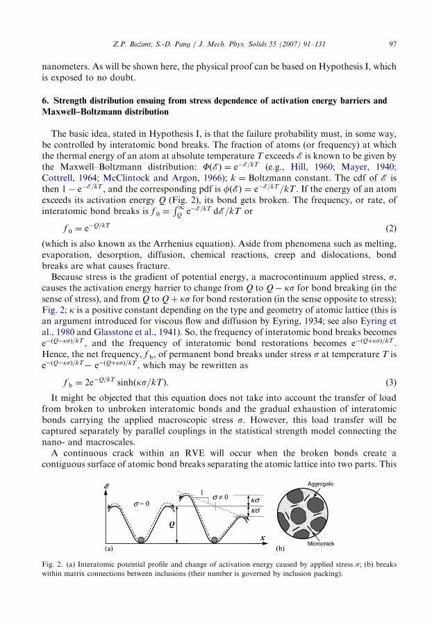
The basic idea, stated in Hypothesis I, is that the failure probability must, in some way,be controlled by interatomic bond breaks. The fraction of atoms (or frequency) at whichthe thermal energy of an atom at absolute temperature T exceeds E is known to be given bythe Maxwell–Boltzmann distribution: FðEÞ ¼ e�E=kT (e.g., Hill, 1960; Mayer, 1940;Cottrell, 1964; McClintock and Argon, 1966); k ¼ Boltzmann constant. The cdf of E isthen 1� e�E=kT , and the corresponding pdf is fðEÞ ¼ e�E=kT=kT . If the energy of an atomexceeds its activation energy Q (Fig. 2), its bond gets broken. The frequency, or rate, ofinteratomic bond breaks is f 0 ¼
R1Q
e�E=kT dE=kT or
f 0 ¼ e�Q=kT (2)
(which is also known as the Arrhenius equation). Aside from phenomena such as melting,evaporation, desorption, diffusion, chemical reactions, creep and dislocations, bondbreaks are what causes fracture.
Because stress is the gradient of potential energy, a macrocontinuum applied stress, s,causes the activation energy barrier to change from Q to Q� ks for bond breaking (in thesense of stress), and from Q to Qþ ks for bond restoration (in the sense opposite to stress);Fig. 2; k is a positive constant depending on the type and geometry of atomic lattice (this isan argument introduced for viscous flow and diffusion by Eyring, 1934; see also Eyring etal., 1980 and Glasstone et al., 1941). So, the frequency of interatomic bond breaks becomese�ðQ�ksÞ=kT , and the frequency of interatomic bond restorations becomes e�ðQþksÞ=kT .Hence, the net frequency, f b, of permanent bond breaks under stress s at temperature T ise�ðQ�ksÞ=kT� e�ðQþksÞ=kT , which may be rewritten as
f b ¼ 2e�Q=kT sinhðks=kTÞ. (3)
It might be objected that this equation does not take into account the transfer of loadfrom broken to unbroken interatomic bonds and the gradual exhaustion of interatomicbonds carrying the applied macroscopic stress s. However, this load transfer will becaptured separately by parallel couplings in the statistical strength model connecting thenano- and macroscales.
A continuous crack within an RVE will occur when the broken bonds create acontiguous surface of atomic bond breaks separating the atomic lattice into two parts. This
Fig. 2. (a) Interatomic potential profile and change of activation energy caused by applied stress s; (b) breakswithin matrix connections between inclusions (their number is governed by inclusion packing).
ARTICLE IN PRESS
0.0
0.5
1.0
00.0
0.5
1.0
0 2 24 4
Cb=0.1 Cb=0.1
p b(�
)kT
/�
F (�)
Tail = Cb��/kT
Constant = Cb
��/kT ��/kT(a) (b)
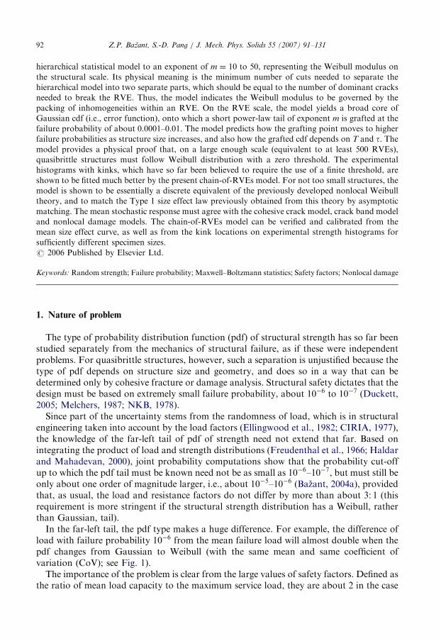
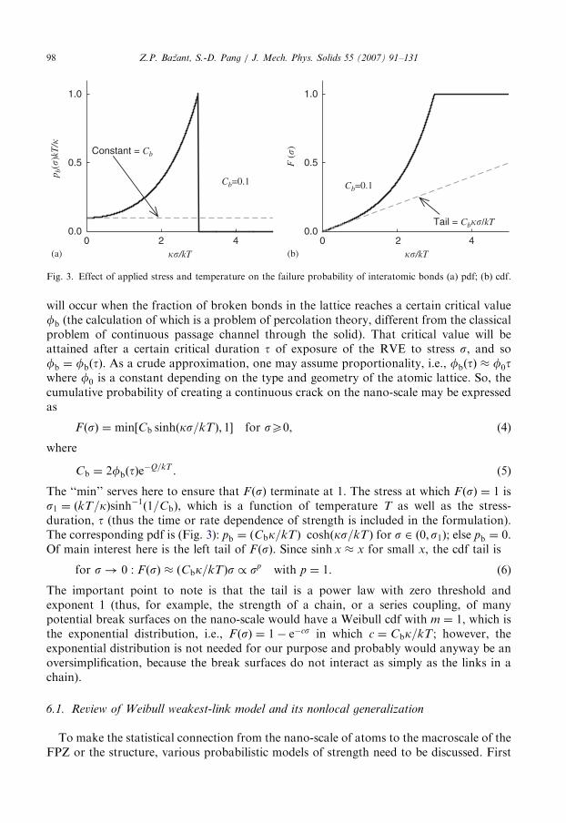
Fig. 3. Effect of applied stress and temperature on the failure probability of interatomic bonds (a) pdf; (b) cdf.
Z.P. Bazant, S.-D. Pang / J. Mech. Phys. Solids 55 (2007) 91–13198
will occur when the fraction of broken bonds in the lattice reaches a certain critical valuefb (the calculation of which is a problem of percolation theory, different from the classicalproblem of continuous passage channel through the solid). That critical value will beattained after a certain critical duration t of exposure of the RVE to stress s, and sofb ¼ fbðtÞ. As a crude approximation, one may assume proportionality, i.e., fbðtÞ � f0twhere f0 is a constant depending on the type and geometry of the atomic lattice. So, thecumulative probability of creating a continuous crack on the nano-scale may be expressedas
F ðsÞ ¼ min½Cb sinhðks=kTÞ; 1� for sX0, (4)
where
Cb ¼ 2fbðtÞe�Q=kT . (5)
The ‘‘min’’ serves here to ensure that F ðsÞ terminate at 1. The stress at which F ðsÞ ¼ 1 iss1 ¼ ðkT=kÞsinh�1ð1=CbÞ, which is a function of temperature T as well as the stress-duration, t (thus the time or rate dependence of strength is included in the formulation).The corresponding pdf is (Fig. 3): pb ¼ ðCbk=kTÞ coshðks=kTÞ for s 2 ð0;s1Þ; else pb ¼ 0.Of main interest here is the left tail of F ðsÞ. Since sinh x � x for small x, the cdf tail is
for s! 0 : F ðsÞ � ðCbk=kTÞs / sp with p ¼ 1. (6)
The important point to note is that the tail is a power law with zero threshold andexponent 1 (thus, for example, the strength of a chain, or a series coupling, of manypotential break surfaces on the nano-scale would have a Weibull cdf with m ¼ 1, which isthe exponential distribution, i.e., F ðsÞ ¼ 1� e�cs in which c ¼ Cbk=kT ; however, theexponential distribution is not needed for our purpose and probably would anyway be anoversimplification, because the break surfaces do not interact as simply as the links in achain).
6.1. Review of Weibull weakest-link model and its nonlocal generalization
To make the statistical connection from the nano-scale of atoms to the macroscale of theFPZ or the structure, various probabilistic models of strength need to be discussed. First
ARTICLE IN PRESSZ.P. Bazant, S.-D. Pang / J. Mech. Phys. Solids 55 (2007) 91–131 99
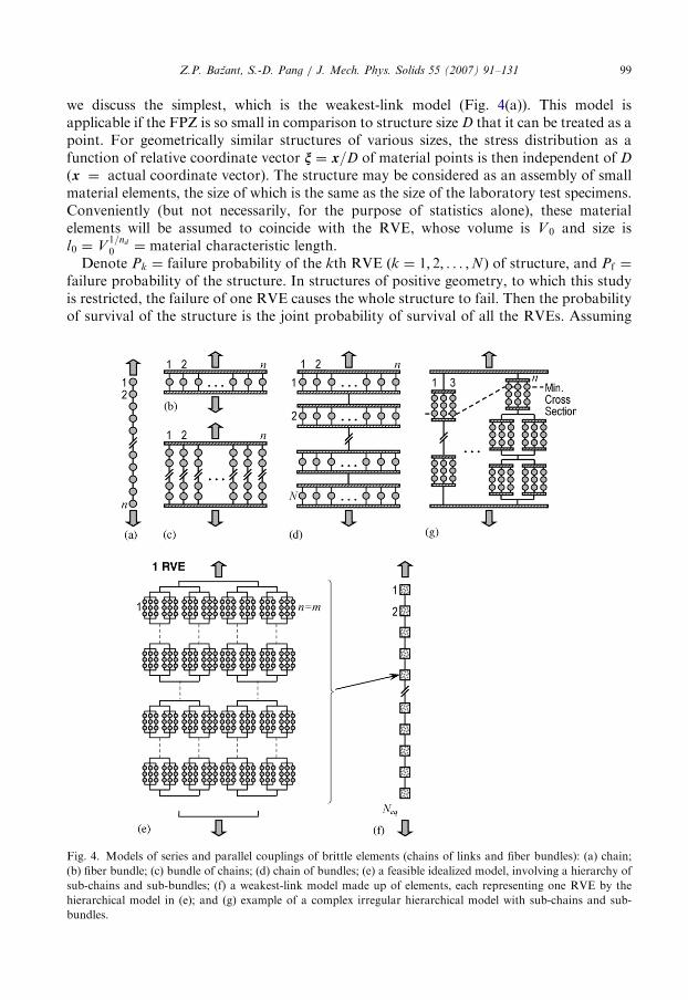
we discuss the simplest, which is the weakest-link model (Fig. 4(a)). This model isapplicable if the FPZ is so small in comparison to structure size D that it can be treated as apoint. For geometrically similar structures of various sizes, the stress distribution as afunction of relative coordinate vector n ¼ x=D of material points is then independent of D
(x ¼ actual coordinate vector). The structure may be considered as an assembly of smallmaterial elements, the size of which is the same as the size of the laboratory test specimens.Conveniently (but not necessarily, for the purpose of statistics alone), these materialelements will be assumed to coincide with the RVE, whose volume is V 0 and size isl0 ¼ V
1=nd
0 ¼ material characteristic length.Denote Pk ¼ failure probability of the kth RVE ðk ¼ 1; 2; . . . ;NÞ of structure, and Pf ¼
failure probability of the structure. In structures of positive geometry, to which this studyis restricted, the failure of one RVE causes the whole structure to fail. Then the probabilityof survival of the structure is the joint probability of survival of all the RVEs. Assuming
Fig. 4. Models of series and parallel couplings of brittle elements (chains of links and fiber bundles): (a) chain;
(b) fiber bundle; (c) bundle of chains; (d) chain of bundles; (e) a feasible idealized model, involving a hierarchy of
sub-chains and sub-bundles; (f) a weakest-link model made up of elements, each representing one RVE by the
hierarchical model in (e); and (g) example of a complex irregular hierarchical model with sub-chains and sub-
bundles.
ARTICLE IN PRESSZ.P. Bazant, S.-D. Pang / J. Mech. Phys. Solids 55 (2007) 91–131100
that all Pk are statistically uncorrelated, we thus have 1� Pf ¼ ð1� P1Þð1� P2Þ � � �
ð1� PN Þ, or
lnð1� Pf Þ ¼XN
k¼1
lnð1� PkÞ � �XN
k¼1
Pk, (7)
where we set lnð1� PkÞ � �Pk because a long chain must fail as Pk51. Based onexperiments, Weibull (1939, 1951) realized that, to fit test data, the left (low probability)tail of the cdf of RVE strength (i.e., failure probability of one RVE) must be a power law,i.e.,
Pk ¼ ½sðxkÞ=s0�m for small sðxkÞ, (8)
where s0 and m are material constants called the scale parameter and Weibull modulus (orshape parameter); and sðxkÞ is the positive part of the maximum principal stress at a pointof coordinate vector xk (the positive part is taken because negative normal stresses do notcause tensile fracture). Substituting this into (7) and making a limit transition from discretesum to an integral over structure volume V, one gets the well-known Weibull probabilityintegral:
� lnð1� Pf Þ ¼X
k
sðxkÞ
s0
� �m
�
ZV
sðxÞs0
� �mdV ðxÞ
lnd
0
. (9)
The integrand ½sðxkÞ=s0�m=lnd
0 ¼ cf ðxÞ is called the spatial concentration of failureprobability and is the continuum equivalent of Pk per volume lnd
0 . Because the structurestrength depends on the minimum strength value in the structure, which is always small ifthe structure is large, the validity of Eq. (9) for large enough structures is unlimited.Consider now geometrically similar structures of different sizes D in which the
dimensionless stress fields sðnÞ are the same functions of dimensionless coordinate vectorn ¼ x=D, i.e., depend only on structure geometry but not on structure size D. In Eq. (9), wemay then substitute sðxÞ ¼ sN sðnÞ where sN ¼ nominal stress ¼ P=bD; P ¼ applied loador a conveniently defined load parameter, and b ¼ structure width (which may but neednot be scaled with D). Further we may set dV ðxÞ ¼ Dnd dV ðnÞ where nd ¼ number ofspatial dimensions in which the structure is scaled (nd ¼ 1; 2 or 3). After rearrangements,Eq. (9) yields � lnð1� Pf Þ ¼ ðsN=S0Þ
m, or
Pf ¼ 1� e�ðsN=s0ÞmCðD=l0Þ
nd¼ 1� e�ðsN=S0Þ
m
, (10)
where
S0 ¼ s0ðl0=DÞnd=mC�1=m; C ¼Z
V
½sðnÞ�m dV ðnÞ. (11)
According to Eq. (10), the tail probability is a power law:
Pf � ðsN=S0Þmðfor sN ! 0Þ. (12)
For Pfp 0.02 (or 0.2), its deviation from Eq. (10) is o1% (or o10%) of Pf .The effect of structure geometry is embedded in integral C, independent of structure
size. Because exponent m in this integral is typically around 25, the regions of structure inwhich the stress is less than about 80% of mean material strength have a negligible effect.
ARTICLE IN PRESSZ.P. Bazant, S.-D. Pang / J. Mech. Phys. Solids 55 (2007) 91–131 101
Note that Pf depends only on the parameter
s�0 ¼ s0lnd=m0 (13)
and not on s0 and l0 separately. So, the material characteristic length l0 is used here onlyfor convenience, to serve as a chosen unit of measurement. The Weibull statistical theoryof strength, per se, has no characteristic length (which is manifested by the fact that thescaling law for the mean strength is a power law; Bazant, 2002). However, in thegeneralization to the probabilistic-energetic theory of failure and size effect (Eq. (25),the use of material characteristic length is essential, which is why introducing l0 is hereconvenient.
The last expression in Eq. (10) is the Weibull cdf in standard form, with scale parameterS0. From Eq. (11) one finds that
sN ¼ C0 ðl0=DÞnd=m, (14)
where
C0 ¼ CfC�1=m; Cf ¼ s0½� lnð1� Pf Þ�1=m. (15)
This equation, in which C0 and S0 are independent of D, describes the scaling of nominalstrength of structure for a given failure probability Pf . The mean nominal strength iscalculated as sN ¼
R10 sNpf ðsN ÞdsN where pf ðsN Þ ¼ dPf ðsN Þ=dsN ¼ pdf of structural
strength. Substituting Eq. (10), one gets, after rearrangements, the well-known Weibullscaling law for the mean nominal strength as a function of structure size D and geometryparameter C;
sNðD;CÞ ¼ s0Gð1þ 1=mÞ ¼ CsðCÞD�nd=m, (16)
where
CsðCÞ ¼ Gð1þ 1=mÞlnd=m0 s0=C1=m (17)
in which one may use the approximation Gð1þ 1=mÞ � 0:63661=m for 5pmp50 (Bazantand Planas, 1998, Eq. 12.1.22).
The CoV of sN is calculated as o2N ¼ ½
R10 s2N dPf ðsN Þ�=s2N � 1. Substitution of Eq. (10)
gives, after rearrangements, the following well-known expression:
oN ¼
ffiffiffiffiffiffiffiffiffiffiffiffiffiffiffiffiffiffiffiffiffiffiffiffiffiffiffiffiffiffiffiffiffiffiGð1þ 2=mÞ
G2ð1þ 1=mÞ� 1
s(18)
which is independent of structure size as well as geometry. Approximately, oN �
ð0:462þ 0:783mÞ�1 for 5pmp50 (Bazant and Planas, 1998, Eq. 12.1.28).It is conceptually useful to introduce the equivalent number, Neq, of RVEs for which a
chain with Neq links gives the same cdf. For a chain under the same tensile stress s ¼ sN ineach element, we have
Pf ¼ 1� e�NeqðsN=s0Þm
. (19)
Setting this equal to (10) and solving for N, we obtain
Neq ¼ ðs0=S0Þm¼ ðD=l0Þ
ndC. (20)
ARTICLE IN PRESSZ.P. Bazant, S.-D. Pang / J. Mech. Phys. Solids 55 (2007) 91–131102
Neq is here a more convenient alternative to what is called the Weibull stress (Beremin,1983), sW, which is defined by setting
Pf ¼ 1� e�ðsW=s0Þm
¼ 1� e�ðV eff=V0ÞðsN=s0Þm
, (21)
where V eff=V0 ¼ ðD=l0ÞndC. Equating this to (10), we see that
sW ¼ sN C1=mðD=l0Þnd=m¼ sNN1=m
eq (22)
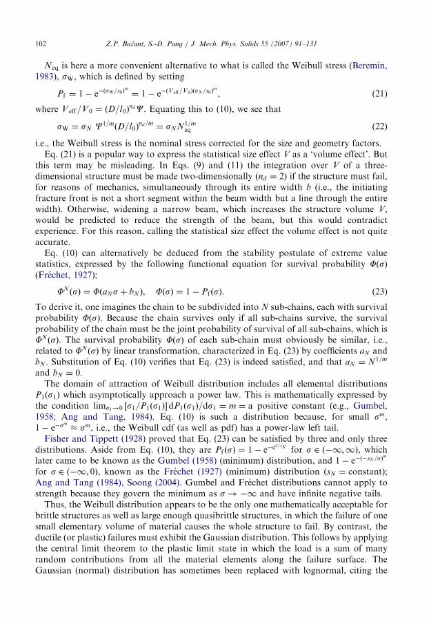
i.e., the Weibull stress is the nominal stress corrected for the size and geometry factors.Eq. (21) is a popular way to express the statistical size effect V as a ‘volume effect’. But
this term may be misleading. In Eqs. (9) and (11) the integration over V of a three-dimensional structure must be made two-dimensionally ðnd ¼ 2Þ if the structure must fail,for reasons of mechanics, simultaneously through its entire width b (i.e., the initiatingfracture front is not a short segment within the beam width but a line through the entirewidth). Otherwise, widening a narrow beam, which increases the structure volume V,would be predicted to reduce the strength of the beam, but this would contradictexperience. For this reason, calling the statistical size effect the volume effect is not quiteaccurate.Eq. (10) can alternatively be deduced from the stability postulate of extreme value
statistics, expressed by the following functional equation for survival probability FðsÞ(Frechet, 1927);
FN ðsÞ ¼ FðaNsþ bN Þ; FðsÞ ¼ 1� Pf ðsÞ. (23)
To derive it, one imagines the chain to be subdivided into N sub-chains, each with survivalprobability FðsÞ. Because the chain survives only if all sub-chains survive, the survivalprobability of the chain must be the joint probability of survival of all sub-chains, which isFN ðsÞ. The survival probability FðsÞ of each sub-chain must obviously be similar, i.e.,related to FN ðsÞ by linear transformation, characterized in Eq. (23) by coefficients aN andbN . Substitution of Eq. (10) verifies that Eq. (23) is indeed satisfied, and that aN ¼ N1=m
and bN ¼ 0.The domain of attraction of Weibull distribution includes all elemental distributions
P1ðs1Þ which asymptotically approach a power law. This is mathematically expressed bythe condition lims1!0 ½s1=P1ðs1Þ�dP1ðs1Þ=ds1 ¼ m ¼ a positive constant (e.g., Gumbel,1958; Ang and Tang, 1984). Eq. (10) is such a distribution because, for small sm,1� e�s
m
� sm, i.e., the Weibull cdf (as well as pdf) has a power-law left tail.Fisher and Tippett (1928) proved that Eq. (23) can be satisfied by three and only three
distributions. Aside from Eq. (10), they are Pf ðsÞ ¼ 1� e�es=sN for s 2 ð�1;1Þ, which
later came to be known as the Gumbel (1958) (minimum) distribution, and 1� e�ð�sN=sÞm
for s 2 ð�1; 0Þ, known as the Frechet (1927) (minimum) distribution ðsN ¼ constantÞ;Ang and Tang (1984), Soong (2004). Gumbel and Frechet distributions cannot apply tostrength because they govern the minimum as s!�1 and have infinite negative tails.Thus, the Weibull distribution appears to be the only one mathematically acceptable for
brittle structures as well as large enough quasibrittle structures, in which the failure of onesmall elementary volume of material causes the whole structure to fail. By contrast, theductile (or plastic) failures must exhibit the Gaussian distribution. This follows by applyingthe central limit theorem to the plastic limit state in which the load is a sum of manyrandom contributions from all the material elements along the failure surface. TheGaussian (normal) distribution has sometimes been replaced with lognormal, citing the
ARTICLE IN PRESSZ.P. Bazant, S.-D. Pang / J. Mech. Phys. Solids 55 (2007) 91–131 103
impossibility of negative strength values. However, this argument is false since, accordingto the central limit theorem, the negative strength values must always lie beyond the reachof the Gaussian core of pdf. Besides, the lognormal distribution has the wrong skewness,opposite to Weibull. Moreover, a lognormal distribution would mean that the load is aproduct, rather than a sum, of the contributions from all the elements along the surface, anobvious impossibility. Thus, the log-normal distribution has no place in strength statistics.
Note that all the extreme value distributions presume the elemental properties to bestatistically independent (uncorrelated). This is always a good enough hypothesis forstructures sufficiently larger than the autocorrelation length la of the strength field,although a rescaled mean strength of RVE is needed. But if la can be taken equal to theRVE size l0, which seems to be quite logical, no rescaling is needed.
If material failure in tension is considered, Eq. (19) is contingent upon the assumptionthat the random material strength is the same for each spatial direction, i.e., that thestrengths in the three principal stress directions are perfectly correlated. Then it is justifiedto interpret s in Eq. (19) as the positive part of the maximum principal nonlocal stress ateach continuum point. However, if the random strengths in the principal directions at thesame continuum point were statistically independent, then s in Eq. (19) would have to bereplaced by
P3I¼1 sI where sI are the positive parts of the principal nonlocal stresses at
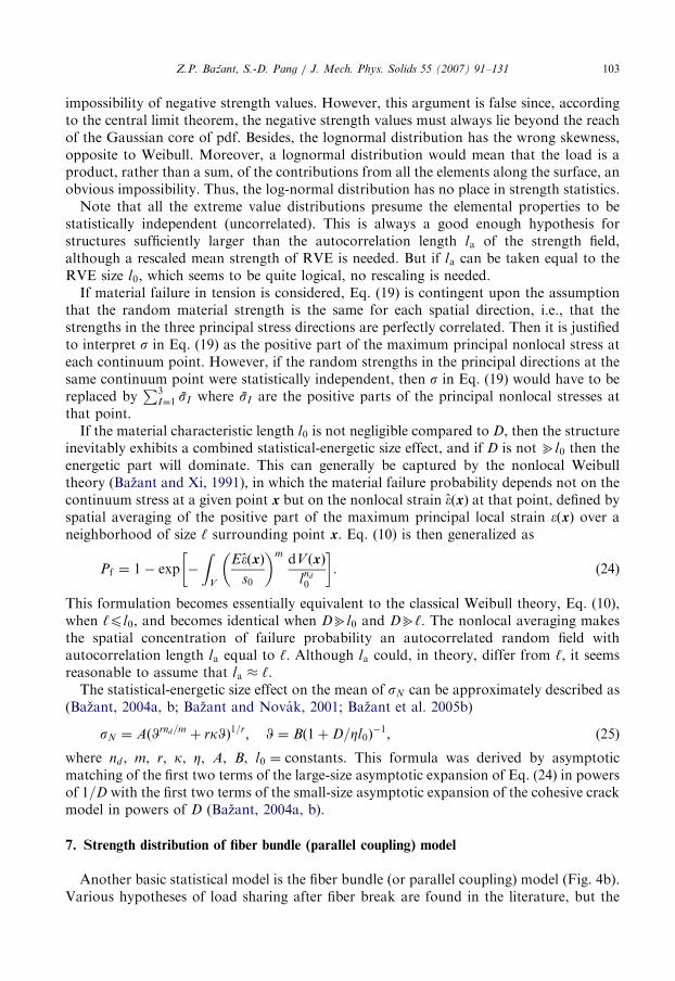
that point.If the material characteristic length l0 is not negligible compared to D, then the structure
inevitably exhibits a combined statistical-energetic size effect, and if D is not bl0 then theenergetic part will dominate. This can generally be captured by the nonlocal Weibulltheory (Bazant and Xi, 1991), in which the material failure probability depends not on thecontinuum stress at a given point x but on the nonlocal strain �ðxÞ at that point, defined byspatial averaging of the positive part of the maximum principal local strain �ðxÞ over aneighborhood of size ‘ surrounding point x. Eq. (10) is then generalized as
Pf ¼ 1� exp �
ZV
E�ðxÞ
s0
� �mdV ðxÞ
lnd
0
� �. (24)
This formulation becomes essentially equivalent to the classical Weibull theory, Eq. (10),when ‘pl0, and becomes identical when Dbl0 and Db‘. The nonlocal averaging makesthe spatial concentration of failure probability an autocorrelated random field withautocorrelation length la equal to ‘. Although la could, in theory, differ from ‘, it seemsreasonable to assume that la � ‘.
The statistical-energetic size effect on the mean of sN can be approximately described as(Bazant, 2004a, b; Bazant and Novak, 2001; Bazant et al. 2005b)
sN ¼ AðWrnd=mþ rkWÞ1=r; W ¼ Bð1þD=Zl0Þ
�1, (25)
where nd , m, r, k, Z, A, B, l0 ¼ constants. This formula was derived by asymptoticmatching of the first two terms of the large-size asymptotic expansion of Eq. (24) in powersof 1=D with the first two terms of the small-size asymptotic expansion of the cohesive crackmodel in powers of D (Bazant, 2004a, b).
7. Strength distribution of fiber bundle (parallel coupling) model
Another basic statistical model is the fiber bundle (or parallel coupling) model (Fig. 4b).Various hypotheses of load sharing after fiber break are found in the literature, but the
ARTICLE IN PRESS
(a) (b) (c)
�0
� � �
�� �
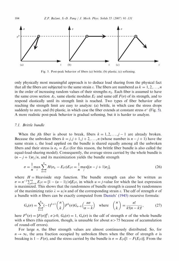
Fig. 5. Post-peak behavior of fibers (a) brittle; (b) plastic; (c) softening.
Z.P. Bazant, S.-D. Pang / J. Mech. Phys. Solids 55 (2007) 91–131104
only physically most meaningful approach is to deduce load sharing from the physical factthat all the fibers are subjected to the same strain �. The fibers are numbered as k ¼ 1; 2; . . . ; nin the order of increasing random values of their strengths sk. Each fiber is assumed to havethe same cross section Af , same elastic modulus Ef and same cdf F ðsÞ of its strength, and torespond elastically until its strength limit is reached. Two types of fiber behavior afterreaching the strength limit are easy to analyze: (a) brittle, in which case the stress dropssuddenly to zero, and (b) plastic, in which case the fiber extends at constant stress s� (Fig. 5).A more realistic post-peak behavior is gradual softening, but it is harder to analyze.
7.1. Brittle bundle
When the jth fiber is about to break, fibers k ¼ 1; 2; . . . ; j � 1 are already broken.Because the unbroken fibers k ¼ j; j þ 1; j þ 2; . . . ; n (whose number is n� j þ 1) have thesame strain �, the load applied on the bundle is shared equally among all the unbrokenfibers and their stress is sk ¼ Ef� (for this reason, the brittle fiber bundle is also called theequal-load-sharing model). Consequently, the average stress carried by the whole bundle isðn� j þ 1Þsj=n, and its maximization yields the bundle strength
s ¼1
nmax�
Xn
k¼1
Hðsk � Ef�ÞEf� ¼1
nmax
j½ðn� j þ 1Þsj�, (26)
where H ¼ Heaviside step function. The bundle strength can also be written ass ¼ n�1
Pnk¼u Ef� ¼ ½1� ðu� 1Þ=n�Ef�, in which u ¼ j-value for which the last expression
is maximized. This shows that the randomness of bundle strength is caused by randomnessof the maximizing ratio l ¼ u=n and of the corresponding strain �. The cdf of strength s ofa bundle with n fibers can be exactly computed from Daniels’ (1945) recursive formula:
GnðsÞ ¼Xn
k¼1
ð�1Þkþ1n
k
� �FkðsÞGn�k
nsn� k
� �where
n
k
� �¼
n!
k!ðn� kÞ!, (27)
here FkðsÞ ¼ ½F ðsÞ�k; sX0, G0ðsÞ ¼ 1, GnðsÞ is the cdf of strength s of the whole bundlewith n fibers (this equation, though, is unusable for about n475 because of accumulationof round-off errors).For large n, the fiber strength values are almost continuously distributed. So, for
n!1, the area fraction occupied by unbroken fibers when the fiber of strength s isbreaking is 1� F ðsÞ, and the stress carried by the bundle is s ¼ Ef�½1� F ðEf�Þ�. From the
ARTICLE IN PRESSZ.P. Bazant, S.-D. Pang / J. Mech. Phys. Solids 55 (2007) 91–131 105
condition ds=d� ¼ 0, the value s ¼ s� ¼ Ef�� for which this expression attains a maximumcan be easily determined. Since the pdf of infinite bundle is symmetric (Daniels, 1945), themaximum must be equal to the mean strength of the bundle, which is ms ¼ s�½1� F ðs�Þ�.
Daniels (1945) proved that, for large n, the variance of the total load on the bundleapproaches ns�2F ðs�Þ½1� F ðs�Þ�. It follows that the CoV of the strength of a large bundlehas the asymptotic approximation
os � r0n�1=2 with r0 �
ffiffiffiffiffiffiffiffiffiffiffiffiffiffiffiffiffiffiffiffiffiffiffiffiffiffiffiffiffiffiffiffiffiffiffiffiF ðs�Þ=½1� F ðs�Þ�
pðfor large nÞ, (28)
where r0 ¼ constant. Hence, os vanishes for n!1. In other words, the strength of aninfinite bundle is deterministic. So (unlike the chain of many elements), the number ofelements (or fibers) in the bundle must be finite and the question is how many of themshould be considered. It will be shown that this number cannot exceed the value of Weibullmodulus m of a RVE.
A question crucial for reliability of very large structures is the shape of the far-left taillying outside the Gaussian core of the pdf of bundle strength when n is finite. Obviously,the left tail cannot be Gaussian because a Gaussian cdf (i.e., the error function) has aninfinite negative tail whereas the bundle strength cannot be negative. The distance from themean ms to the point s ¼ 0, which is a point sure to lie beyond the Gaussian core, may bewritten as DsnG ¼ ms ¼ ds=os ¼ ðds=r0Þ
ffiffiffinp
, where ds ¼ osms ¼ standard deviation ofbundle strength. The spread DsG of the Gaussian core (i.e., the distance from the mean tothe end of Gaussian core) must obviously be smaller than this; it is found to be alsoproportional to
ffiffiffinp
, i.e.,
DsG ¼ gGdsffiffiffinp
, (29)
where gG is some constant less than 1=r0. Smith (1982) showed that Daniels’ Gaussianapproximation to the cdf of bundle has the convergence rate of at least Oðn�1=6Þ, which is arather slow convergence, and proposed an improved Gaussian approximation with a meandepending on n, for which the convergence rate improves but still is not guaranteed to bebetter than Oðn�1=3ðlog nÞ2Þ.
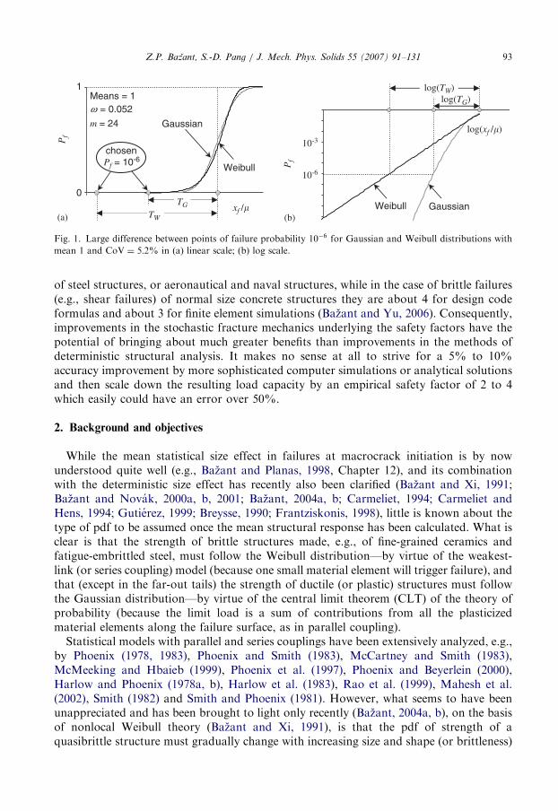
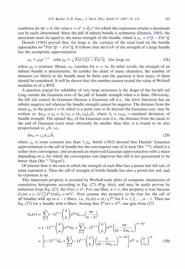
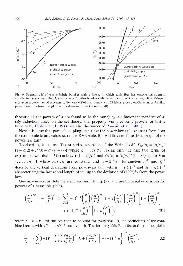
Of interest here is the case in which the strength of each fiber has a power-law left tail, ofsome exponent p. Then the cdf of strength of brittle bundle has also a power-law tail, andits exponent is np.
This important property is revealed by Weibull-scale plots of computer simulations ofcumulative histograms according to Eq. (27) (Fig. 6(a)), and may be easily proven byinduction from Eq. (27). Set F ðsÞ ¼ sp. For one fiber, n ¼ 1, this property is true becauseG1ðsÞ ¼ ð�1Þ
2 11
F1ðsÞG0 ¼ ðspÞ
1. Now assume this property to be true for the cdf ofall bundles with up to n� 1 fibers, i.e., GkðsÞ ¼ ðs=skÞ
kp for k ¼ 1; 2; . . . ; n� 1. Then useEq. (27) for a bundle with n fibers. Noting that F kðsÞ ¼ skp, one gets from (27)
GnðsÞ ¼Xn
k¼1
ð�1Þkþ1n
k
!skpGn�k
nsn� k
� �
¼ ð�1Þnþ1n
n
!snpG0 þ
Xn�1k¼1
ð�1Þkþ1n
k
!skp nsðn� kÞsn�k
� �ðn�kÞp
¼ ð�1Þnþ1G0 þXn�1k¼1
ð�1Þkþ1n
k
!n
ðn� kÞsn�k
� �ðn�kÞp" #
snp ¼ssn
� �np
ð30Þ
ARTICLE IN PRESS
0.10
0.20
0.30
0.40
0.50
0.60
0.70
0.80
0.90
0.0 0.4 0.8 1.2-80
-60
-40
-20
0
-5 -3 -1ln (�/s0) �/s0
n=2
3
6
12
24
ln[ l
n(1-
Gn)
]
1
24
Bundle cdf in Weibull
probability paper
(each fiber: p = 1)
Bundle cdf in Gaussian
probability paper
(each fiber: p = 1)
n=2
361224
Φ-1
(Pf)
G
(a) (b)
Fig. 6. Strength cdf of elastic–brittle bundles with n fibers, in which each fiber has exponential strength
distribution; (a) curves of logðPf Þ versus logs for fiber bundles with increasing n, in which a straight line of slope p
represents a power law of exponent p; (b) exact cdf of fiber bundle with 24 fibers, plotted on Gaussian probability
paper (deviation from straight line is a deviation from Gaussian pdf).
Z.P. Bazant, S.-D. Pang / J. Mech. Phys. Solids 55 (2007) 91–131106
(because all the powers of s are found to be the same); sn is a factor independent of s.(By induction based on the set theory, this property was previously proven for brittlebundles by Harlow et al., 1983; see also the works of Phoenix et al., 1997.)Now it is clear that parallel couplings can raise the power-law tail exponent from 1 on
the nano-scale to any value, m, on the RVE scale. But will this yield a realistic length of thepower-law tail?To check it, let us use Taylor series expansion of the Weibull cdf; F wbðsÞ ¼ ðs=s1Þ
p
ð1� x=2!þ x2=3!� x3=4!þ � � �Þ where x ¼ ðs=s1Þp. Taking only the first two terms of
expansion, we obtain F ðsÞ ¼ ðs=s1Þpð1� sp=t1Þ and GkðsÞ ¼ ðs=skÞ
kpð1� sp=tkÞ for k ¼
1; 2; . . . ; n� 1 where s1; sk; tk are constants and t1 ¼ 21=ps1. Parameters t1=p1 and t
1=p
k
describe the vertical deviations from power-law tail, with d1 ¼ t1ð�Þ1=p and dk ¼ tkð�Þ
1=p
characterizing the horizontal length of tail up to the deviation of ð100�Þ% from the powerlaw.One may now substitute these expressions into Eq. (27) and use binomial expansions for
powers of a sum; this yields
ssn
� �np
1�stn
� �p� ��Xn�1k¼1
ð�1Þkþ1n
k
!ss1
� �kp
1� kst1
� �p� �nsjsj
!jp
1�nsjtj
!p" #
þ ð�1Þnþ1ss1
� �np
1þ nst1
� �p� �, ð31Þ
where j ¼ n� k. For this equation to be valid for every small s, the coefficients of the com-bined terms with snp and snpþ1 must vanish. The former yields Eq. (30), and the latter yields
t1
tn
¼Xn�1k¼1
ð�1Þkþ1n
k
� �n
j
s1
sj
� �jp
k þn
j
t1
tj
� �p� �þ ð�1Þnþ1n
( )1=psn
s1
� �n
. (32)
ARTICLE IN PRESS
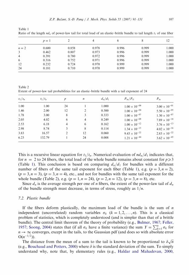
Table 1
Ratio of the length ndn of power-law tail for total load of an elastic–brittle bundle to tail length t1 of one fiber
p ¼ 1 2 4 6 8 12
n ¼ 2 0.600 0.858 0.978 0.996 0.999 1.000
3 0.462 0.807 0.973 0.996 0.999 1.000
4 0.391 0.780 0.972 0.996 0.999 1.000
6 0.316 0.752 0.971 0.996 0.999 1.000
12 0.232 0.724 0.970 0.999 0.999 1.000
24 0.181 0.710 0.970 0.999 0.999 1.000
Table 2
Extent of power-law tail probabilities for an elastic–brittle bundle with a tail exponent of 24
s1=sn t1=tn p n dn=d1 Ptn=Pt1 Ptn
1.00 1.00 24 1 1.000 1:00� 10�00 3:00� 10�01
1.46 2.00 12 2 0.500 1:00� 10�04 5:50� 10�05
1.78 3.00 8 3 0.333 1:00� 10�07 1:30� 10�07
2.05 4.02 6 4 0.249 1:00� 10�09 7:89� 10�10
2.53 6.18 4 6 0.162 1:00� 10�12 3:76� 10�13
2.98 8.74 3 8 0.114 1:34� 10�15 4:02� 10�16
3.83 16.57 2 12 0.060 9:43� 10�22 2:83� 10�22
6.23 132.79 1 24 0.008 1:21� 10�44 3:62� 10�45
Z.P. Bazant, S.-D. Pang / J. Mech. Phys. Solids 55 (2007) 91–131 107
This is a recursive linear equation for t1=tn. Numerical evaluation of ndn=d1 indicates that,for n ¼ 2 to 24 fibers, the total load of the whole bundle remains about constant for pX3(Table 1). This conclusion is based on comparing dn=d1 for bundles with a differentnumber of fibers of the same tail exponent for each fiber (Table 1), e.g. ðp ¼ 3; n ¼ 2Þ,ðp ¼ 3; n ¼ 3Þ, ðp ¼ 3; n ¼ 4Þ, etc., and not for bundles with the same tail exponent for thewhole bundle (Table 2), e.g. ðp ¼ 1; n ¼ 24Þ, ðp ¼ 2; n ¼ 12Þ, ðp ¼ 3; n ¼ 8Þ, etc.
Since dn is the average strength per one of n fibers, the extent of the power-law tail of dn
of the bundle strength must decrease, in terms of stress, roughly as 1=n.
7.2. Plastic bundle
If the fibers deform plastically, the maximum load of the bundle is the sum of n
independent (uncorrelated) random variables sk ðk ¼ 1; 2; . . . ; nÞ. This is a classicalproblem of statistics, which is completely understood (and is simpler than that of a brittlebundle). The central limit theorem of the theory of probability (e.g., Bulmer, 1967; Feller,1957; Soong, 2004) states that (if all sk have a finite variance) the sum Y ¼
Pnk¼1 sk for
n!1 converges, except in the tails, to the Gaussian pdf (and does so with absolute errorOðn�1=2Þ).
The distance from the mean of a sum to the tail is known to be proportional to dffiffiffinp
(e.g., Bouchaud and Potters, 2000) where d is the standard deviation of the sum. To simplyunderstand why, note that, by elementary rules (e.g., Haldar and Mahadevan, 2000,
ARTICLE IN PRESSZ.P. Bazant, S.-D. Pang / J. Mech. Phys. Solids 55 (2007) 91–131108
p. 150), the mean and variance of the maximum load of the bundle are mn ¼ nms ands2n ¼ ns2s where ms and s2s are the mean and variance of sk. If all sk are nonnegative, m mustbe nonnegative, too, even though the Gaussian pdf has an infinite negative tail. Of course,the Gaussian pdf of tensile strength cannot apply within the range of negative s; hence, theGaussian core cannot reach farther from the mean mn than to the distance of rsn wherer ¼ nms=
ffiffiffiffiffiffiffins2s
p¼ o�1n ¼ o�10
ffiffiffinp
, with o0 denoting the CoV of one fiber.The tail outside the Gaussian core and the tails of sk are known to be of the same type
(Bouchaud and Potters, 2000); i.e., if the tail of fibers is a power-law, so is the tail of themean. To explain this and other tail properties, consider a bundle of two plastic ‘fibers’with stresses y and z, and tail cdf of strength:
GðyÞ ¼y
y0
� �jp
1�y
tj
� �p� �; HðzÞ ¼
z
z0
� �kp
1�z
tk
� �p� �, (33)
where j; k; p; y0; z0 are positive constants, and parameter t defines the power-law tail lengthsuch that ð100�Þ% deviations from each power-law tail occur at d ¼ t�1=p (note that whenj ¼ k ¼ 1, GðyÞ and HðzÞ describe the first two terms of the expansion of Weibull cdf). Bydifferentiation, the corresponding pdf tails are
gðyÞ ¼jp
yo
y
y0
� �jp�1
1�y
t0j
!p" #; hðzÞ ¼
kp
z0
z
z0
� �kp�1
1�z
t0k
� �p� �, (34)
where
t0j ¼ tj
jp
jpþ p
� �1=p
; t0k ¼ tk
kp
kpþ p
� �1=p
. (35)
The maximum load on the bundle is x ¼ yþ z. Load x can be obtained by all possiblecombinations of forces y and z ¼ x� y in the first and second fibers, which both must be attheir strength limit if the bundle load is maximum. So, according to the joint probabilitytheorem, the pdf of the sum x is
f ðxÞ ¼
Z x
0
gðyÞhðx� yÞdy
¼ jkp2y�jp0 z
�kp0
Z x
0
yjp�1ðx� yÞkp�1 1�y
t0j
!p" #1�
x� y
t0k
� �p" #
dy. ð36Þ
Although the standard approach in the theory of probability would be to take the Laplacetransform of the above convolution integral and later invert it, a conceptually simplerpower series approach will suffice for our purpose. We expand ðx� yÞkp�1 and ðx� yÞp
according to the binomial theorem and, upon integrating, we retain only two leading termsof the power series expansion of f ðxÞ. This yields
f ðxÞ �jkp2C00
yjp0 z
kp0
1� C0px
t0j
!p
� C0qx
t0k
� �p" #
xjpþkp�1 ðerror / xðjþkþ2Þp�1Þ, (37)
where
C00 ¼GðjpÞGðkpÞ
Gðjpþ kpÞ; C0p ¼
Gðjpþ kpÞGðpþ jpÞ
GðjpÞGðjpþ kpþ pÞ; C0q ¼
Gðjpþ kpÞGðpþ kpÞ
GðkpÞGðjpþ kpþ pÞ. (38)
ARTICLE IN PRESSZ.P. Bazant, S.-D. Pang / J. Mech. Phys. Solids 55 (2007) 91–131 109
The corresponding cdf of the maximum load on the bundle of two fibers is
F ðxÞ �x
x0
� �ðjþkÞp
1�x
t�
� �ph i, (39)
where
x�ðjþkÞp0 ¼
C00
yjp0 z
kp0
jkp
ðj þ kÞ; ðt�Þ�p
¼C0pðj þ 1Þðj þ kÞ
jtpj ðj þ k þ 1Þ
þC0qðk þ 1Þðj þ kÞ
ktpkðj þ k þ 1Þ
. (40)
So we conclude that the exponents of fiber tails in a plastic bundle are additive, while thelength of the power-law tail of the cdf of the total load of the bundle decreases fromd1 ¼ t1�1=p to dtn ¼ t��1=p. In the case of fibers with p ¼ 1, a bundle of three fibers is acoupling of one fiber with a bundle of two fibers, which gives dtn=d1 ¼ 0:667; a bundle offour fibers is a coupling of one fiber with a bundle of three fibers, which givesdtn=d1 ¼ 0:625, etc., and for 24 fibers dtn=d1 ¼ 0:521.
The cdf of the average strength of each fiber is simply a horizontal scaling of the cdf forthe total load on the bundle, and so Eq. (39) can be written in terms of s:
F ðsÞ ¼nsx0
� �ðjþkÞp
1�nst�
� �ph i¼
ssn
� �np
1�stn
� �p� �, (41)
where sn ¼ x0=n, tn ¼ t�=n and n ¼ j þ k. So we see that the total load, as well as theaverage strength of the bundle, has a cdf tail with exponent np, which is the same as for abrittle bundle. The length of the power-law tail of the cdf of the strength of a bundle (i.e.,the load per fiber), which is dn ¼ dtn=n, gets changed, for � ¼ 0:15, by factors 0:667=3 ¼0:222 and 0:521=24 ¼ 0:022, respectively, with p ¼ 1.
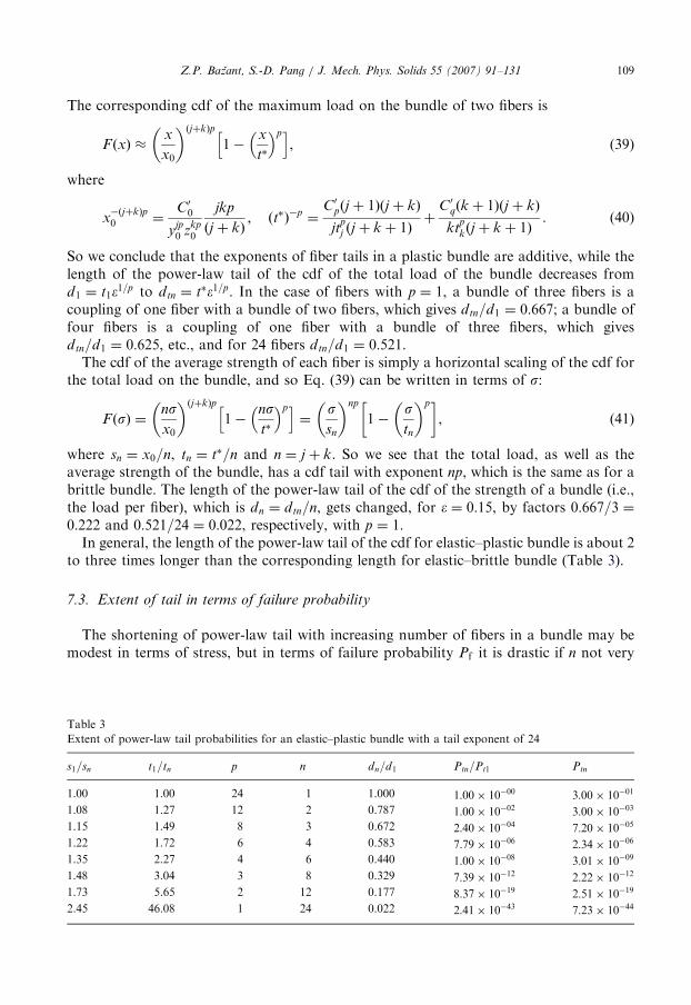
In general, the length of the power-law tail of the cdf for elastic–plastic bundle is about 2to three times longer than the corresponding length for elastic–brittle bundle (Table 3).
7.3. Extent of tail in terms of failure probability
The shortening of power-law tail with increasing number of fibers in a bundle may bemodest in terms of stress, but in terms of failure probability Pf it is drastic if n not very
Table 3
Extent of power-law tail probabilities for an elastic–plastic bundle with a tail exponent of 24
s1=sn t1=tn p n dn=d1 Ptn=Pt1 Ptn
1.00 1.00 24 1 1.000 1:00� 10�00 3:00� 10�01
1.08 1.27 12 2 0.787 1:00� 10�02 3:00� 10�03
1.15 1.49 8 3 0.672 2:40� 10�04 7:20� 10�05
1.22 1.72 6 4 0.583 7:79� 10�06 2:34� 10�06
1.35 2.27 4 6 0.440 1:00� 10�08 3:01� 10�09
1.48 3.04 3 8 0.329 7:39� 10�12 2:22� 10�12
1.73 5.65 2 12 0.177 8:37� 10�19 2:51� 10�19
2.45 46.08 1 24 0.022 2:41� 10�43 7:23� 10�44
ARTICLE IN PRESSZ.P. Bazant, S.-D. Pang / J. Mech. Phys. Solids 55 (2007) 91–131110
small. The Pf value at the terminal point of power-law tail gets reduced in the ratio:
rP ¼Ptn
Pt1
¼ðdn=snÞ
np
ðd1=s1Þ¼
tns1
t1sn
� �np
ð2�Þn�1. (42)
Thus, for the brittle or plastic case, respectively, we have, in terms of Pf , the followingreduction ratios for the tail terminal point:
for two fibers and p ¼ 12 : rP ¼ 1:8� 10�4 or 1:0� 10�2,
for three fibers and p ¼ 8 : rP ¼ 4:3� 10�7 or 2:4� 10�4,
for six fibers and p ¼ 4 : rP ¼ 1:3� 10�12 or 1:0� 10�8,
for 24 fibers and p ¼ 1 : rP ¼ 1:2� 10�44 or 2:4� 10�43. (43)
Obviously, for the same number of fibers, the shortening of the power-law tail is for brittlefibers (Table 2) much stronger than for plastic fibers (Table 3) in small bundles, but not inlarge bundles. For softening fibers (Fig. 5(c)), intermediate behavior may be expected.According to the aforementioned values, not even two fibers with m ¼ 24 power-law tail
up to Pt1 ¼ 0:3 could produce a power-law tail of a bundle reaching up to Ptn ¼ 0:003,which is the tail length needed to satisfy Hypothesis II, because analysis of chains withvarious numbers of RVEs shows that a power law-tail of one RVE reaching up to Pt1 ¼
0:003 produces a Weibull cdf up to Ptn ¼ 0:8, 0.9 and 0.95 for 500, 750 and 1000 RVEs,respectively. When the number of RVEs 4500, the cdf on the Weibull probability paper isvisually hardly distinguishable from a straight line (Fig. 8(b)).Therefore, if the tail of the bundle should extend up to Pf ¼ 0:003, it is necessary for the
cdf of two plastic fibers in the bundle to be Weibull up to at least P1 ¼ 0:3 (computersimulations, too, confirm it). The power-law tail of the cdf of bundle strength, terminatesat
Ptn � �n tn
sn
� �np
¼ P nt1
s1
sn
tn
t1
� �np
, (44)
where Pt1 ¼ �ðt1=s1Þp¼ failure probability at the terminal point of the power-law tail of
one fiber. For a bundle with plastic fibers, the ratio ðtns1Þ=ðt1snÞ decreases approximately asn�1=p, with an error of o3%, which leads to a shrinking of Ptn as ðPt1=nÞn. To wit, if thepower-law tail of one fiber ends at Pt1 ¼ 0:3, the tails of bundles with a tail exponent ofm ¼ np ¼ 24 for three or eight fibers terminate at Pf � 7:2� 10�5 or 2:2� 10�12.Obviously, the power-law tail of the strength of any bundle with more than about threefibers is, from the practical viewpoint, nonexistent. Accurate computer simulations confirmthat (see Table 3).From this we may conclude that if the power-law tail of one fiber strength terminates at
Pt1 ¼ 0:3, then the tail of bundle strength (total load per fiber) with tail exponent 24,terminates at Pf ¼ 3:0� 10�3, 7:2� 10�5 and 7:2� 10�44, respectively, if n ¼ 2, 3 or 24.The last value is so small that the power-law tail can have no effect in reality.
ARTICLE IN PRESSZ.P. Bazant, S.-D. Pang / J. Mech. Phys. Solids 55 (2007) 91–131 111
7.4. Basic properties of softening, brittle and plastic bundles
Of main practical interest is a bundle of softening fibers. Because the softening isintermediate between plastic and brittle responses (Fig. 5(c)), those properties that arecommon to both brittle and plastic bundles may be assumed to hold also for bundles withsoftening fibers. They may be summarized as follows.
Theorem 1. For brittle, plastic, and probably also softening, fibers, the exponents of power-
law tail of cdf of fibers in a bundle (or parallel coupling) are additive. The power-law tail
exponent of strength cdf of a chain is the smallest power-law tail exponent among all links in
the chain (or series coupling). Parallel coupling reduces the length of power-law tail of cdf
(within one order of magnitude for up to 10 fibers, and up to two orders of magnitude for up to
24 fibers). But the extent of the tail in terms of failure probability can decrease by many more
orders of magnitude when the power-law tail exponent of the bundle is high. If the power-law
tail exponent of each fiber is high ð410Þ, it is possible to couple in parallel no more than two
non-brittle (plastic or, probably, softening) fibers if a nonnegligible power-law tail of a bundle
should be preserved.
8. Extreme value statistics of RVE and of quasibrittle structure
According to Eq. (7), the failure probability of a chain of Neq identical links with failureprobability P1ðsÞ can be exactly calculated as Pf ðsÞ ¼ 1� ½1� P1ðsÞ�Neq . Hence,
Neq ¼logð1� Pf Þ
logð1� P1Þ. (45)
If the chain of N links is characterized by Weibull cdf up about Pf ¼ 0:80, the wholeexperimental cumulative histogram with typical scatter is, on the Weibull probabilitypaper, visually indistinguishable from Weibull cdf. If the limit of power-law tail of the cdfof one link (one RVE) in a chain is Pt1 ¼ 0:003 (which is a tail hardly detectable inexperiments), the equivalent number Neq of RVEs in the structure (or links in the chain)must be, according to Eq. (45), approximately
NeqX500 (46)
in order to produce for the chain a cdf indistinguishable from Weibull. For concretespecimens, as it appears, statistical samples with Neq4500 do not exist. However, test datafor fine-grained ceramics cover this kind of size, and they show a distinctly Weibull cdf(e.g., Weibull, 1939; Bansal et al. 1976a, b; Ito et al., 1981; Katayama and Hattori, 1982;Matsusue et al., 1982; Soma et al., 1985; Ohji, 1988; Amar et al., 1989; Hattori et al., 1989;Bruhner-Foit and Munz, 1989; Quinn, 1990; Quinn and Morrell, 1991; Katz et al., 1993;Gehrke et al., 1993; Danzer and Lube, 1996; Sato et al., 1996; Lu et al., 2002a; Santoset al., 2003). This justifies Hypothesis II. Therefore, it is logical to assume that a RVE ofany quasibrittle material that becomes brittle on the large scale of application should havea power-law tail extending roughly up to Pt1 � 0:003.
One microcrack in a RVE, or too few of them, would not cause the RVE, and thus thewhole structure, to fail (which is, of course, why the RVE cannot be assumed to behave
ARTICLE IN PRESSZ.P. Bazant, S.-D. Pang / J. Mech. Phys. Solids 55 (2007) 91–131112
statistically as a chain). Rather, a certain number of separate microcracks must form tocause the RVE to fail, which is statistically the same situation as in a bundle of parallelfibers. This number, n, obviously depends on the packing of dominant aggregate pieces inconcrete, or the packing of dominant grains in a ceramic or rock, or generally the packingof dominant heterogeneities in the material.So, the RVE must be considered to behave statistically as a bundle (Fig. 4(b)), and the
structure (of positive geometry) as a chain of such bundles (Fig. 4(d)). However, canthe RVE be modelled by Daniels’ bundle of fibers, or is it necessary to consider that theelements of the bundle consist of chains, sub-bundles, sub-chains, sub-sub-bundles, etc.? Itis argued that the latter must be the case.As additional support for the hypothesis that a RVE of quasibrittle material must
behave as a bundle (series coupling), two points should be noted: (i) If the allegedRVE behaved as a chain (series) coupling, the failure would localize into an elementof the chain and the actual RVE would be smaller than the alleged RVE. (ii) Sinceconcrete microstructure is brittle, the cdf of strength of small laboratory specimenscould not appear as Gaussian (Hypothesis III) if parallel coupling statistics did notapply. Yet majority of experiments for concrete show this cdf to be in fact approxi-mately Gaussian, except in the undetectable tails (Julian, 1955; Shalon and Reintz,1955; Rusch et al., 1969; Erntroy, 1960; Neaman and Laguros, 1967; Metcalf, 1970; Mirzaet al., 1979; Bartlett and MacGregor, 1996; FHWA, 1998; Chmielewski and Konopka,1999).Consider now a chain of RVEs (Fig. 4(f)). The cdf of strength of each RVE has a
power-law cdf tail, and so a long enough chain will follow the Weibull cdf. How manylinks (i.e., RVEs) are needed to attain Weibull distribution for the whole chain (orstructure)?If the structural model were a chain of bundles (Harlow et al., 1983), each bundle would
have, for concrete, 24 parallel fibers of tail exponent 1, and, as has been shown, this wouldyield for each bundle a tail extending only up to the probability Pf � 10�45. This meansthat the chain would have to consist of about 1047 bundles for the Weibull distribution toget manifested (a chain of that many RVEs, each of the size of 0.1m, would have to reachbeyond the most distant galaxies!). So, if each RVE were modelled by Daniels’ bundle of m
fibers with activation energy based cdf ðp ¼ 1Þ, the Weibull cdf would never be observed inpractice. Yet it is (Weibull, 1939).Based on experience (Weibull, 1939), it may be assumed (Hypothesis II) that the cdf of a
positive geometry structure in which the number N of RVEs is about 1000 should be muchcloser to Weibull than to Gaussian distribution (whether N should rather be 104 is, ofcourse, debatable, but it definitely cannot be orders of magnitude larger). To obtain forsuch N a cdf that is experimentally indistinguishable from Weibull, the power-law tail ofcdf of each RVE must, according to Eq. (45), extend up to at least Pf � 0:003. To this end,the bundle with m ¼ 24 must contain no more than two parallel fibers (each of which, withtail exponent 12), must almost completely follow Weibull distribution, and must be ofplastic or softening type.A tail below Pf ¼ 0:003 does not get manifested in graphical cumulative histograms and
cannot be directly confirmed by any of the existing test data from small laboratoryspecimens that are not much larger than a RVE (a cumulative histogram of at least 104
identical tests would be needed to reveal such a tail on Weibull probability paper). Neithercan the Weibull cdf for 1000 RVEs be checked for concrete, because large enough
ARTICLE IN PRESSZ.P. Bazant, S.-D. Pang / J. Mech. Phys. Solids 55 (2007) 91–131 113
specimens have not been tested. Nevertheless, confirmation can be obtained from theexisting experimental data for specimens of fine-grained ceramics, which contain at least1000 RVEs. Indeed, they follow the Weibull distribution closely (Weibull, 1939; Bansalet al. 1976a, b; Ito et al., 1981; Katayama and Hattori, 1982; Matsusue et al., 1982; Somaet al., 1985; Ohji, 1988; Amar et al., 1989; Hattori et al., 1989; Bruhner-Foit and Munz,1989; Quinn, 1990; Quinn and Morrell, 1991; Katz et al., 1993; Gehrke et al., 1993; Danzerand Lube, 1996; Sato et al., 1996; Lu et al., 2002a; Santos et al., 2003).
The length of power-law tail of the cdf of RVE is found to strongly depend on whethereach of the parallel fibers is brittle or plastic. Brittle fibers never give a sufficiently longpower-law tail for the cdf of a RVE, even for just two parallel fibers with tail exponent 12(required to obtain m ¼ 24). A long enough power-law tail of RVE, extending up toPf ¼ 0:003 (Hypothesis II), is obtained for a bundle of two plastic fibers, and doubtlessalso for a bundle of softening fibers with a sufficiently mild softening slope. This has beenverified by computer simulations, and also follows from the aforementioned general rulesfor the length of power-law cdf tails of bundles.
Based on Hypotheses II and III, and within the context of activation energy theory(Hypothesis I), it follows from the foregoing analysis that a power-law tail of exponentsuch as m ¼ 24, extending up to Pf ¼ 0:003, can be achieved for an RVE only with ahierarchical statistical model involving both parallel and series couplings, as idealized inFig. 4(e). The first bundle (parallel coupling) must involve not more than two parallelelements, and each of them may then consist of a hierarchy of sub-chains of sub-bundles ofsub-sub-chains of sub-sub-bundles, etc. The load-deflection diagrams of the sub-chains,sub-sub-chains, etc., cannot be perfectly brittle, i.e., must be plastic or softening. If theconstituents of the RVE are not plastic, as in the case of concrete, rocks or ceramics,elements behaving plastically are, of course, unrealistic. Hence, the elements of thehierarchical statistical model should in reality be softening. At any scale of microstructure,a softening behavior is engendered by distributed microcracking on a lower-level sub-scaleeven if every constituent on that sub-scale is brittle.
In the hierarchical statistical model exemplified in Fig. 4(e), the elements of identicalpower-law tails, coupled in each sub-chain, serve to extend the power-law tail and, if longenough, will eventually produce Weibull cdf while the tail exponent remains unchanged.On the next higher scale, the parallel coupling of two or three of these sub-chains in a sub-bundle will raise their tail exponent by summation but will shorten the power-law tailsignificantly. Then, on the next higher scale of microstructure, a series coupling of manysub-bundles in a chain will again extend the power-law tail, and a parallel coupling of twoof these chains will again raise the tail exponent and shorten the power-law tailsignificantly, until the macroscale of an RVE is reached.
The actual behavior of a RVE will, of course, correspond to some irregular hierarchicalmodel, such as that shown in Fig. 4(g). In that case, according to the aforementioned basicproperties, the exponent of the power-law tail for the RVE, and thus the Weibull modulusof a large structure, is determined by the minimum cross section, defined as the sectionwith the minimum number of cuts of elementary serial bonds that are needed to separatethe model into two halves.
Because random variations in the couplings of the hierarchical model for extreme valuestatistics of RVE must be expected, it would make hardly any sense to compute thestructural failure probability directly from activation energy controlled interatomicbonds characterized by power-law cdf tail of exponent 1. Nevertheless, establishing the
ARTICLE IN PRESSZ.P. Bazant, S.-D. Pang / J. Mech. Phys. Solids 55 (2007) 91–131114
hierarchical model that provides a statistical connection of RVE strength to the stressdependence of activation energy barriers of interatomic bonds has five benefits:
1.
It proves that the cdf of RVE strength must have a power-law tail. 2. It proves that a sufficiently long tail, extending up to Pf � 0:0001–0.01, and the Weibulldistribution of strength of a large enough structure, are physically justifiable.
3. It proves that the Weibull distribution must have a zero threshold. 4. It provides the dependence of Weibull scale parameter s0 on temperature T and oncharacteristic load duration t (or on the loading rate, which is characterized by 1=t).
5. It indicates that the complicated transition between the power-law tail and the Gaussiancore can be considered to be short (because, with only two or three elements coupled inparallel, the power-law tail reaches far enough).
Point 4, according to Eqs. (6) and (10), means that the scaling parameter S0 of theWeibull cdf of structural strength must depend on absolute temperature T and on loadduration t (or loading rate 1=t), and that the dependence must have the form:
S0 ¼ S0r
T
T0
fbðt0ÞfbðtÞ
eð1=T�1=T0ÞQ=k, (47)
where T0 ¼ reference absolute temperature (e.g., room temperature 298�K), t0 ¼ referenceload duration (or time to reach failure of the specimen, e.g., 1min), and S0r ¼ referencevalue of S0 corresponding to T0 and t0. The corresponding Weibull cdf of structuralstrength at any temperature and load duration may be written as
Pf ðsÞ ¼ 1� exp �s
S0r
T0
T
fbðtÞfbðt0Þ
eð1=T0�1=TÞQ=k
� �m� �. (48)
Note, however, that this simple dependence on T is expected to apply only through alimited range of temperatures and load durations. The reason is that the interatomicpotential surface typically exhibits not one but many different activation barriers Q andcoefficients k for different atoms and bonds, with different Q and k dominating in differenttemperature ranges.On the atomic scale, which is separated from the RVE scale of concrete by about eight
orders of magnitude, the breakage of a RVE must involve trillions of interatomic bondbreaks governed by activation energy. Lest one might have doubts about using the activationenergy theory to span so many orders of magnitude, it should be realized that there are manyother similar examples where the activation energy has been successfully used for concrete,rock, composites and ceramics—e.g., the temperature dependence of fracture energy and ofcreep rate of concrete (Bazant and Prat, 1988), the effect of crack growth rate on fractureresistance (Bazant and Jirasek, 1993; Bazant, 1995; Bazant and Li, 1997), or thesoftening–hardening reversal due to a sudden increase of loading rate (Bazant et al., 1995).Activation energy concepts have been used by Zhurkov (1965) and Zhurkov and
Korsukov (1974) in a deterministic theory of structural lifetime as a function of T and s,which corresponds to replacing Eq. (4) by
F ðsÞ ¼ min½ðCb=2Þeks=kT ; 1� for sX0. (49)
The corresponding pdf, however, has a delta-function spike at s ¼ 0, which isobjectionable. The preceding derivation would lead to this formula if the bond
ARTICLE IN PRESSZ.P. Bazant, S.-D. Pang / J. Mech. Phys. Solids 55 (2007) 91–131 115
restorations, governed by activation energy barrier Qþ ks, were ignored, i.e., if f b ¼
e�ðQ�ksÞ=kT instead of Eq. (3). As a result, this theory incorrectly predicts a solid todisintegrate within a finite lifetime even if s ¼ 0, and it also gives unrealistically shortlifetimes for failures at low stress, i.e., for low failure probabilities and for large structures.Especially, Zhurkov’s theory is incompatible with Weibull theory and could not becombined with the present analysis.
In a similar way as here, the activation energy concept has more recently been used inprobabilistic analysis of the lifetime distribution, based on models of the evolution ofdefects in parallel coupling systems with various assumed simple load-sharing rules; seePhoenix (1978), Phoenix and Tierney (1983), Phoenix and Smith (1983), Curtin and Scher(1997), Phoenix et al. (1997), and Newman and Phoenix (2001). The temperature and stressdependence of lifetime has been related to the interatomic activation energy through anargument traced to Eyring (1936; also Eyring et al., 1980; Glasstone et al., 1941; Tobolsky,1960).
9. Grafted Weibull–Gaussian cdf of one RVE
If the RVE of concrete (with m � 24) were modelled as a bundle of more than two fibers,the transition of its cdf from the Gaussian core to the Weibull (or power-law) tail wouldoccupy several orders of magnitude of Pf . The mathematical formulation of suchtransition region would be complicated. However, as has already been argued, the bundlesand sub-bundles in the hierarchical model for RVE should contain only, near themacroscale, no more than two parallel fibers (with more parallel fibers allowed for scalesclose to nano, where the tail exponent is low). Consequently, the transition region in termsof Pf must be relatively short, happening within one or two orders of magnitude of Pf .
This permits us to assume, for the sake of simplicity, that the transition occursapproximately within a point, sN ;gr. In other words, we may assume that a Weibull pdf tailfW is grafted at one point on the left side onto a Gaussian pdf core fG (i.e., onto the errorfunction). Such a grafted pdf (Bazant and Pang, 2005b), may be mathematically describedas follows:
for sNosN ;gr : p1ðsNÞ ¼ rf ðm=s1ÞðsN=s1Þm�1e�ðsN=s1Þ
m
¼ rffWðsNÞ, (50)
for sNXsN ;gr : p1ðsNÞ ¼ rf e�ðsN�mGÞ
2=2d2G=ðdGffiffiffiffiffiffi2ppÞ ¼ rffGðsNÞ, (51)
where mG, dG ¼ mean and standard deviation of Gaussian core alone; m, s1 ¼ shape andscale parameters of Weibull tail alone. The cdf of the latter is
for BoBgr : P1ðBÞ ¼ rf ð1� e�Bm
Þ,
for BXBgr : P1ðBÞ ¼ rf ð1� e�Bmgr Þ þ
rf
dGn
ffiffiffiffiffiffi2pp
Z B
Bgr
e�ðB0�mGnÞ
2=2d2Gn dB0 (52)
where
rf ¼ ½1� FGðBgrÞ þ FWðBgrÞ��1. (53)
Here mGn ¼ mG=s1; dGn ¼ dG=s1; Bgr ¼ sN ;gr=s1. rf is a scaling factor ensuring that the cdf ofthe Weibull–Gaussian graft be normalized;
R1�1
fðsN ÞdsN ¼ 1. The far-left tail of cdf of
ARTICLE IN PRESSZ.P. Bazant, S.-D. Pang / J. Mech. Phys. Solids 55 (2007) 91–131116
P1 is a power law which can be expressed as
P1 � rf ðsN=s1Þmðfor sN ! 0Þ. (54)
The scale parameter s1 used in the grafting method is related to s0 of Eq. (12) bys0 ¼ r
1=m
f s1. The typical values for rf range between 1.00 and 1.14, which means that s0differs from s1 by less than 0.5%. In practice, r
1=m
f can be taken as 1, and s0 ¼ s1. But rfshould remain in the formulation of P1 (Eq. 52), or else an error of up to 12% in the cdf ofone RVE is likely.Both pdfs, as defined in Eqs. (50) and (51), are matched to be continuous at the grafting
point, Bgr. This gives the compatibility condition:
mGn ¼ Bgr � dGnf�2 ln½ffiffiffiffiffiffi2pp
mdGnBm�1gr e�B
mgr �g1=2. (55)
The probability at which the Weibull tail for one RVE ceases to apply lies within the rangePgr ¼ rfFWðBgrÞ � 0:0001–0.01, and is used to determine the relative length of the Weibulltail Bgr, to be grafted:
Bgr ¼ ½� lnð1� FWðBgrÞÞ�1=m. (56)
If one knows the standard deviation of the Gaussian core dG and the scale parameter s1 ofthe Weibull tail, one can calculate mGn from Eq. (55); dG can be easily determined from the
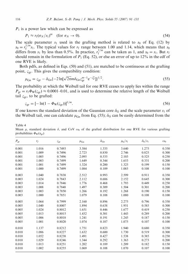
Table 4
Mean m, standard deviation d, and CoV o0 of the grafted distribution for one RVE for various grafting
probabilities FWðagrÞ
Pgr rf Bgr mGn dGn m0=s1 d0=s1 o0
0.001 1.016 0.7493 3.584 1.335 3.640 1.275 0.350
0.001 1.009 0.7496 2.723 0.850 2.746 0.825 0.300
0.001 1.005 0.7496 2.095 0.535 2.103 0.525 0.250
0.001 1.003 0.7499 1.649 0.344 1.653 0.331 0.200
0.001 1.001 0.7499 1.324 0.200 1.325 0.199 0.150
0.001 1.000 0.7499 1.084 0.109 1.085 0.108 0.100
0.003 1.040 0.7838 2.512 0.993 2.599 0.911 0.350
0.003 1.024 0.7843 2.112 0.686 2.152 0.645 0.300
0.003 1.014 0.7846 1.776 0.468 1.793 0.449 0.250
0.003 1.008 0.7848 1.497 0.309 1.504 0.301 0.200
0.003 1.003 0.7850 1.266 0.192 1.268 0.190 0.150
0.003 1.000 0.7851 1.079 0.108 1.080 0.108 0.100
0.005 1.064 0.7999 2.160 0.896 2.275 0.796 0.350
0.005 1.040 0.8007 1.894 0.638 1.951 0.585 0.300
0.005 1.024 0.8012 1.651 0.446 1.677 0.419 0.250
0.005 1.013 0.8015 1.432 0.301 1.443 0.289 0.200
0.005 1.006 0.8018 1.241 0.191 1.245 0.187 0.150
0.005 1.001 0.8020 1.074 0.107 1.075 0.107 0.100
0.010 1.137 0.8212 1.751 0.823 1.940 0.680 0.350
0.010 1.086 0.8227 1.632 0.600 1.730 0.519 0.300
0.010 1.052 0.8238 1.491 0.427 1.538 0.385 0.250
0.010 1.029 0.8246 1.344 0.292 1.363 0.273 0.200
0.010 1.013 0.8251 1.202 0.189 1.209 0.182 0.150
0.010 1.002 0.8255 1.069 0.108 1.070 0.107 0.100
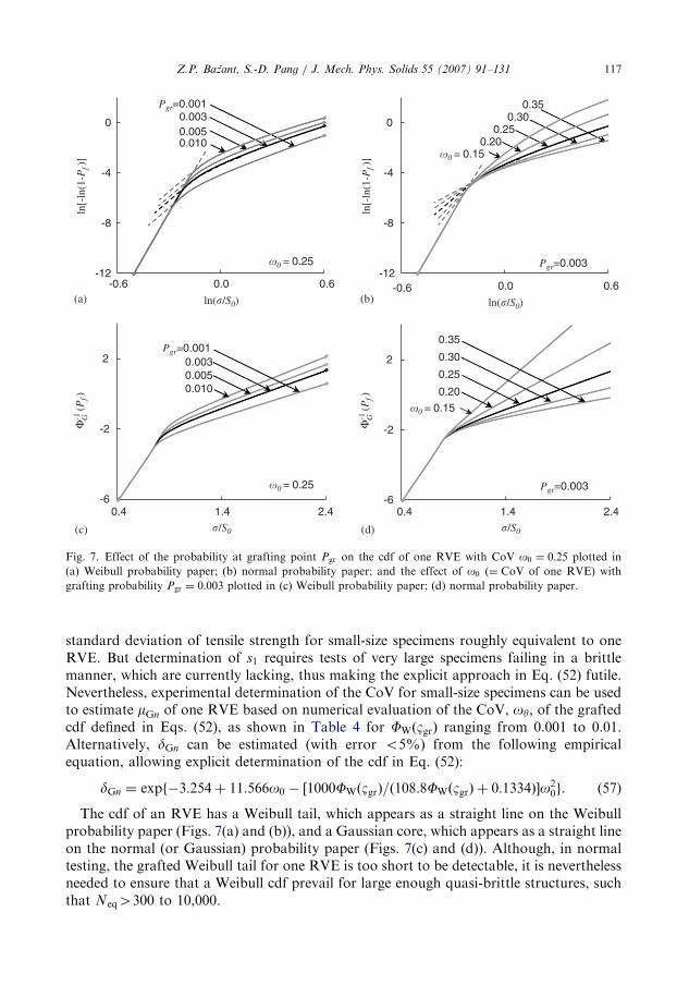
ARTICLE IN PRESS
0.35
0.200.25
0.30
-6
-2
2
-6
-2
2
0.0030.0050.010
0.35
0.20
0.25
0.30
-12
-8
-4
0
-0.6-12
-8
-4
0
-0.6 0.0 0.6
ln(�/S0)0.0 0.6
ln(�/S0)
ln[-
ln(1
-Pf )
]
Pgr=0.003
Pgr=0.003�0 = 0.25
�0 = 0.15
�0 = 0.15
�0 = 0.25
Pgr=0.0010.0030.0050.010
Pgr=0.001
Φ-1
(Pf )
G
ln[-
ln(1
-Pf )
]Φ
-1 (P
f )G
�/S0 �/S0
0.4 1.4 2.4 0.4 1.4 2.4
(a) (b)
(d)(c)
Fig. 7. Effect of the probability at grafting point Pgr on the cdf of one RVE with CoV o0 ¼ 0:25 plotted in
(a) Weibull probability paper; (b) normal probability paper; and the effect of o0 (¼ CoV of one RVE) with
grafting probability Pgr ¼ 0:003 plotted in (c) Weibull probability paper; (d) normal probability paper.
Z.P. Bazant, S.-D. Pang / J. Mech. Phys. Solids 55 (2007) 91–131 117
standard deviation of tensile strength for small-size specimens roughly equivalent to oneRVE. But determination of s1 requires tests of very large specimens failing in a brittlemanner, which are currently lacking, thus making the explicit approach in Eq. (52) futile.Nevertheless, experimental determination of the CoV for small-size specimens can be usedto estimate mGn of one RVE based on numerical evaluation of the CoV, oy, of the graftedcdf defined in Eqs. (52), as shown in Table 4 for FWðBgrÞ ranging from 0.001 to 0.01.Alternatively, dGn can be estimated (with error o5%) from the following empiricalequation, allowing explicit determination of the cdf in Eq. (52):
dGn ¼ expf�3:254þ 11:566o0 � ½1000FWðBgrÞ=ð108:8FWðBgrÞ þ 0:1334Þ�o20g. (57)
The cdf of an RVE has a Weibull tail, which appears as a straight line on the Weibullprobability paper (Figs. 7(a) and (b)), and a Gaussian core, which appears as a straight lineon the normal (or Gaussian) probability paper (Figs. 7(c) and (d)). Although, in normaltesting, the grafted Weibull tail for one RVE is too short to be detectable, it is neverthelessneeded to ensure that a Weibull cdf prevail for large enough quasi-brittle structures, suchthat Neq4300 to 10,000.
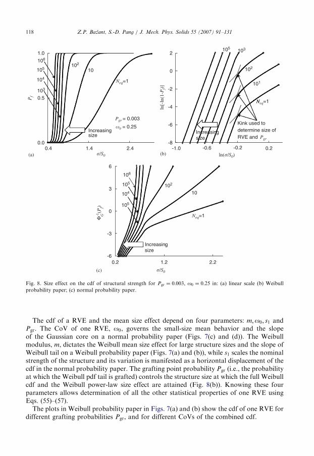
ARTICLE IN PRESS
-6
-3
0
3
6
0.2 1.2 2.2
10
Increasingsize
0.0
0.5
1.0
0.4 1.4 2.4
Pf
Neq=1
Neq=1
Neq=1
10
Pgr = 0.003
�� = 0.25
106
102
105103
102
101
105
104
103
102
106
105
104
105
Kink used to determine size of RVE and Pgr
sizeIncreasingsize
-8
-6
-4
-2
0
2
-1.0 -0.6 -0.2 0.2ln(�/S0)�/S0
�/S0
ln[-
ln(1
-Pf)]
Increasing
Φ-1
(Pf)
G
(a) (b)
(c)
Fig. 8. Size effect on the cdf of structural strength for Pgr ¼ 0:003, o0 ¼ 0:25 in: (a) linear scale (b) Weibull
probability paper; (c) normal probability paper.
Z.P. Bazant, S.-D. Pang / J. Mech. Phys. Solids 55 (2007) 91–131118
The cdf of a RVE and the mean size effect depend on four parameters: m;o0; s1 andPgr. The CoV of one RVE, o0, governs the small-size mean behavior and the slopeof the Gaussian core on a normal probability paper (Figs. 7(c) and (d)). The Weibullmodulus, m, dictates the Weibull mean size effect for large structure sizes and the slope ofWeibull tail on a Weibull probability paper (Figs. 7(a) and (b)), while s1 scales the nominalstrength of the structure and its variation is manifested as a horizontal displacement of thecdf in the normal probability paper. The grafting point probability Pgr (i.e., the probabilityat which the Weibull pdf tail is grafted) controls the structure size at which the full Weibullcdf and the Weibull power-law size effect are attained (Fig. 8(b)). Knowing these fourparameters allows determination of all the other statistical properties of one RVE usingEqs. (55)–(57).The plots in Weibull probability paper in Figs. 7(a) and (b) show the cdf of one RVE for
different grafting probabilities Pgr, and for different CoVs of the combined cdf.
ARTICLE IN PRESSZ.P. Bazant, S.-D. Pang / J. Mech. Phys. Solids 55 (2007) 91–131 119
10. Grafted Weibull–Gaussian cdf for structures equivalent to many RVEs
Since one RVE is defined as a material volume whose failure causes the whole structureto fail, quasibrittle structures that consist of more than one RVE (and have positivegeometry, no notches producing stress singularity and no pre-existing large cracks) behaveas a chain of RVEs (Fig. 4(f)). The chain survives if and only if all the RVEs survive,1� Pf ¼ ð1� P1Þ
Neq , and so the failure probability Pf for nominal stress sN , which is acommon parameter for all the RVEs, is exactly
Pf ðsN Þ ¼ 1� ½1� P1ðsN Þ�Neq , (58)
where P1ðsÞ is the grafted distribution for one RVE. A large enough structure fails at smallenough, sN , and so the cdf of each RVE must be within the power-law tail, P1ðsNÞ ¼
ðsN=s0Þm (Theorem 1). From Eq. (58) and the well-known limit limN!1ð1þ x=NÞN ¼ ex,
it follows that
Pf ðsN Þ1 ¼ 1�NeqðsN=s0Þ
m
Neq
� �Neq
)Neq!1
1� e�NeqðsN=s0Þm
(59)
i.e., the distribution in Eq. (58) becomes Weibull distribution for a structure with a largeenough equivalent number of RVEs.
The transition from Gaussian to Weibull cdf when passing from small to large sizes isevident in Fig. 8. On a linear scale of sN and Pf (Fig. 8(a)), in which the CoV isproportional to the maximum slope of the cdf curve, the CoV first decreases withincreasing Neq, which is typical of bundle (parallel-coupling) statistics, and then stabilizesat a constant value, which is typical of chain (weakest-link) statistics. For Neq41000 andgrafting probability Pgr ¼ 0:001 of one RVE, the cdf is visually indistinguishable fromWeibull cdf and an increase in size causes merely a leftward shift of the cdf curve as a rigidbody.
On the Weibull scale (i.e., Weibull probability paper), on which the Weibull cdf of sN isa straight line, the straight segment lengthens with increasing Neq (Fig. 8(b)) while theGaussian core, appearing as a concave curve, shifts upwards. The transition shows up onthe histogram as a distinctive kink (Fig. 8(b)), the location of which may be preciselydefined as the point of intersection of the extensions of the Gaussian core and the Weibulltail.
On the normal probability paper, on which the Gaussian (normal) cdf of sN appears as astraight line, the straight segment shortens with increasing Neq (Fig. 8(c)), while the tailsegment of Weibull cdf appears as a curve, shifting and changing shape with Neq.
The mean nominal strength (Fig. 9) for any number of RVEs can be determined asfollows:
sN ¼
Z 10
sNNeq½1� P1ðsNÞ�Neq�1p1ðsN ÞdsN . (60)
Analytical evaluation of Eq. (60), with p1ðsNÞ and P1ðsNÞ defined in Eqs. (50)–(51) and(52), respectively, is impossible but the asymptotes can be determined. For large size, theasymptote must be the Weibull size effect, due to the power-law tail of the cdf of each RVE(Hypotheses I and II), which is given by the following expression on a logarithmic scale:
logðsN;W Þ ¼ �ð1=mÞ logðNeqÞ þ log½s0Gð1þ 1=mÞ�. (61)
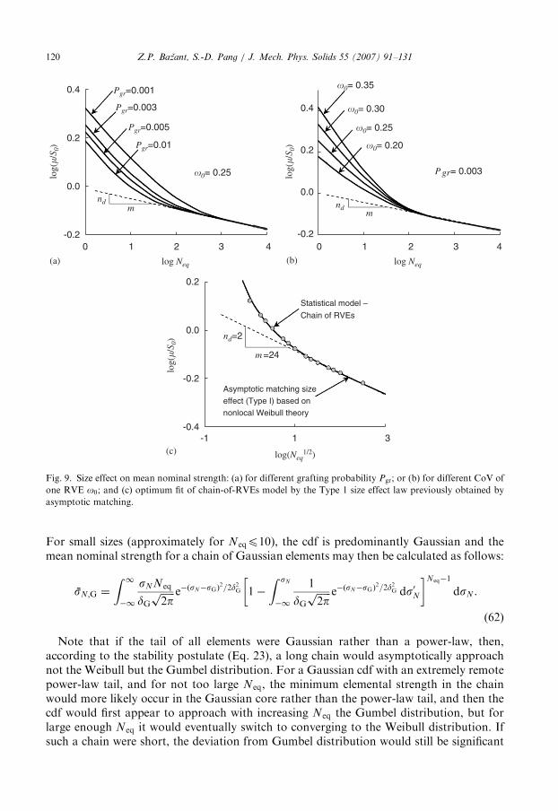
ARTICLE IN PRESS
-0.2
0.0
0.2
0.4
0 1 2 3 4 2 3
log Neq log Neq
log(
�/S 0
)
-0.2
0.0
0.2
0.4
log(
�/S 0
)
0 1 4
Pgr=0.001
Pgr=0.003
Pgr=0.005
Pgr=0.01
Pgr= 0.003
mnd nd
m
-0.4
-0.2
0.0
0.2
-1 1
log(Neq1/2)
log(
�/S 0
)
Asymptotic matching size effect (Type I) based on nonlocal Weibull theory
m =24
nd=2
Statistical model –
Chain of RVEs
�0= 0.25
�0= 0.35
�0= 0.30
�0= 0.25
�0= 0.20
3
(a) (b)
(c)
Fig. 9. Size effect on mean nominal strength: (a) for different grafting probability Pgr; or (b) for different CoV of
one RVE o0; and (c) optimum fit of chain-of-RVEs model by the Type 1 size effect law previously obtained by
asymptotic matching.
Z.P. Bazant, S.-D. Pang / J. Mech. Phys. Solids 55 (2007) 91–131120
For small sizes (approximately for Neqp10), the cdf is predominantly Gaussian and themean nominal strength for a chain of Gaussian elements may then be calculated as follows:
sN;G ¼
Z 1�1
sNNeq
dGffiffiffiffiffiffi2pp e�ðsN�sGÞ
2=2d2G 1�
Z sN
�1
1
dGffiffiffiffiffiffi2pp e�ðsN�sGÞ
2=2d2G ds0N
� �Neq�1
dsN .
(62)
Note that if the tail of all elements were Gaussian rather than a power-law, then,according to the stability postulate (Eq. 23), a long chain would asymptotically approachnot the Weibull but the Gumbel distribution. For a Gaussian cdf with an extremely remotepower-law tail, and for not too large Neq, the minimum elemental strength in the chainwould more likely occur in the Gaussian core rather than the power-law tail, and then thecdf would first appear to approach with increasing Neq the Gumbel distribution, but forlarge enough Neq it would eventually switch to converging to the Weibull distribution. Ifsuch a chain were short, the deviation from Gumbel distribution would still be significant
ARTICLE IN PRESSZ.P. Bazant, S.-D. Pang / J. Mech. Phys. Solids 55 (2007) 91–131 121
and the mean nominal strength would then be expressed as
logðsN;GÞ ¼ mG½1� wðNeqÞðo0=ffiffiffippÞ�, (63)
where wðNeqÞ ¼ 1; 32for Neq ¼ 2; 3, respectively. For intermediate values, 3oNeqo10, an
analytical expression for parameter ms is unavailable (Ang and Tang, 1984). Since evenvery remote Weibull tails of RVEs spoil approach to Gumbel distribution, even for smallNeq, it is necessary that the mean size effect curve in Eq. (60) be obtained by nonlinearregression.
When the asymptotic Weibull strength of Eq. (61) is subtracted from the mean nominalstrength (Eq. 60) in logarithmic scale, the difference fits very well the following empiricalfunction:
logðsNÞ � logðsN ;W Þ ¼ exp½� expða1 � a2 logðNeqÞÞ�, (64)
where
a1 ¼ ln � ln logm0
s0Gð1þ 1=mÞ
� �� �. (65)
Parameter a1 anchors the size effect curve for one RVE; m0 is the mean for one RVE; anda2 controls the rate of transition to Weibull size effect and depends on the length of theWeibull tail for one RVE. Calibrating the mean size effect curve requires identifying atleast four parameters: m0, Pgr, m, and s0.
11. Equivalence to nonlocal Weibull theory
Fig. 9(c) demonstrates another interesting point: The four parameters for the mean sizeeffect, i.e., m0, Pgr, m, and s0, can be optimized to match very accurately the mean Type 1energetic-statistical size effect law in Eq. (25) for nonlocal theory, obtained by asymptoticmatching (Bazant, 2004a, b). This law, in turn, was further shown to match closely theMonte Carlo simulations with the nonlocal Weibull theory (Bazant and Novak, 2000a, b;Bazant, 2002). This match shows that, on the continuum scale, both theories areequivalent.
It would make no sense to use the present discrete model for structure sizes smaller thanone RVE. However, the nonlocal Weibull theory, being a continuum theory, can beextended to structure size D! 0. Although such extension is a mathematical abstractionof no real physical meaning, it has nevertheless been shown mathematically useful. Themean zero-size asymptotic behavior can be easily determined by considering the FPZ to beperfectly plastic, while the large size asymptotics follows from equivalent LEFM or thesmeared-tip model (Bazant, 2002), in which the FPZ shrinks to a point. Thus, thecontinuum theory makes it possible to obtain mean analytical approximation for any D viaasymptotic matching (Bazant, 2004a, b) of the power series expansions, for D! 0 in termsof powers of D, and for !1 in terms of powers of 1=D. Derivation of the Type 1 sizeeffect law in Eq. (25) (Bazant, 1997, 2002) is an example.
The mean size effect behavior of the nonlocal Weibull theory is known to be wellcaptured by the cohesive crack model, crack band model or some of the nonlocal damagemodels for concrete and other quasibrittle materials (Bazant, 2002; Bazant and Planas,1998). For D! 0, these models predict a linear approach in terms of D to a finite
ARTICLE IN PRESSZ.P. Bazant, S.-D. Pang / J. Mech. Phys. Solids 55 (2007) 91–131122
‘zero-size’ nominal strength of structure. On a larger scale, all these models shouldapproximately match the mean strength predictions of the present discrete theory.Consequently, the present theory provides another, statistical, explanation and
justification of nonlocal concepts for materials with softening damage or cohesivefracture. In the nonlocal Weibull theory, however, the cdf of strength of the nonlocalaveraging volume cannot be predicted and must be assumed. On the basis of the presenttheory, it may be assumed as the Gaussian cdf with a grafted power-law tail.
12. Verification and calibration
One way to calibrate the present theory is to observe the kink point locations on theexperimental histograms of strength of specimens with two sufficiently different Neq ¼
Neq1 and Neq2, corresponding to sufficiently different specimen sizes D ¼ D1 and D2, andpossibly to different geometries characterized by C ¼ C1 and C2. The specimens must notbe too large, so that the kinks are clearly detectable on the histograms. Plotting thehistogram on both Weibull and normal probability papers, one can then obtain theWeibull and Gaussian segments of cdf by linear regression of the straight segments ofthe histograms on each of these two papers. Each histogram may be approximated by a cdfconsisting of two semi-infinite segments, Weibull on the left and Gaussian on the right.These segments intersect at a precise kink point, labelled as ðsN i;Pf iÞ where 1 ¼ 1; 2; . . .(Fig. 8(b)). The failure probability at each kink point must be equal to the joint survivalprobability of all the RVEs subjected to the same sN ; this yields:
1� Pf i ¼ ½1� P1ðsN iÞ�Neq i ; Neqi ¼ ðDi=l0ÞCi ði ¼ 1; 2Þ. (66)
Because the stress at each kink point, and thus in each RVE, must be small enough to lie inthe power-law tail of cdf of one RVE, we also have P1ðsN iÞ ¼ rf ðsN i=s1Þ
mði ¼ 1; 2Þ where
rf is a known value, rf � 1. Substituting this expression into the foregoing equation,one gets two equations from which l0 can be eliminated. Thus one obtains, afterrearrangements:
lnð1� Pf 1Þ
lnð1� Pf 2Þ¼
D1C1 ln½1� ðsN1=s0Þm�
D2C2 ln½1� ðsN2=s0Þm�, (67)
where s0 ¼ r1=mf s1 � s1. This is a nonlinear equation, from which s1 can be solved by
Newton iterations, and l0 may then be easily solved from Eq. (66).Alternatively, one may eliminate s0, and this yields for l0 the nonlinear equation:
1� ð1� Pf 1Þl0=D1C1
1� ð1� Pf 2Þl0=D2C2
¼sN1
sN2
� �m
(68)
from which l0 can be solved by Newton iterations; s0 may then be easily solved fromEq. (66).The grafting point probability for one RVE is then obtained as
Pgr ¼ ðsN i=s0Þm¼ rf ðsN i=s1Þ
mði ¼ 1 or 2Þ. (69)
According to experience with nonlocal models, the size l0 of one RVE can be roughlyestimated as the double or triple of the maximum size of material inhomogeneities. Then itis sufficient to calibrate the model from an experimental strength histogram for one sizeonly ði ¼ 1Þ.
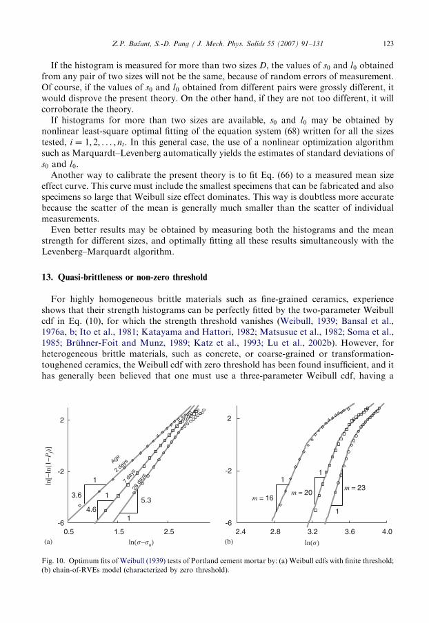
ARTICLE IN PRESSZ.P. Bazant, S.-D. Pang / J. Mech. Phys. Solids 55 (2007) 91–131 123
If the histogram is measured for more than two sizes D, the values of s0 and l0 obtainedfrom any pair of two sizes will not be the same, because of random errors of measurement.Of course, if the values of s0 and l0 obtained from different pairs were grossly different, itwould disprove the present theory. On the other hand, if they are not too different, it willcorroborate the theory.
If histograms for more than two sizes are available, s0 and l0 may be obtained bynonlinear least-square optimal fitting of the equation system (68) written for all the sizestested, i ¼ 1; 2; . . . ; nt. In this general case, the use of a nonlinear optimization algorithmsuch as Marquardt–Levenberg automatically yields the estimates of standard deviations ofs0 and l0.
Another way to calibrate the present theory is to fit Eq. (66) to a measured mean sizeeffect curve. This curve must include the smallest specimens that can be fabricated and alsospecimens so large that Weibull size effect dominates. This way is doubtless more accuratebecause the scatter of the mean is generally much smaller than the scatter of individualmeasurements.
Even better results may be obtained by measuring both the histograms and the meanstrength for different sizes, and optimally fitting all these results simultaneously with theLevenberg–Marquardt algorithm.
13. Quasi-brittleness or non-zero threshold
For highly homogeneous brittle materials such as fine-grained ceramics, experienceshows that their strength histograms can be perfectly fitted by the two-parameter Weibullcdf in Eq. (10), for which the strength threshold vanishes (Weibull, 1939; Bansal et al.,1976a, b; Ito et al., 1981; Katayama and Hattori, 1982; Matsusue et al., 1982; Soma et al.,1985; Bruhner-Foit and Munz, 1989; Katz et al., 1993; Lu et al., 2002b). However, forheterogeneous brittle materials, such as concrete, or coarse-grained or transformation-toughened ceramics, the Weibull cdf with zero threshold has been found insufficient, and ithas generally been believed that one must use a three-parameter Weibull cdf, having a
-6
-2
2
0.5 1.5 2.5 2.8 3.2 3.6 4.02.4ln(�−�u) ln(�)
ln[−
ln(1
−Pf)]
-6
-2
2
m = 16
11
1
3.6
1
4.6
15.3
1
m = 20m = 23
Age
2 day
s
7 da
ys28
day
s
(a) (b)
Fig. 10. Optimum fits of Weibull (1939) tests of Portland cement mortar by: (a) Weibull cdfs with finite threshold;
(b) chain-of-RVEs model (characterized by zero threshold).
ARTICLE IN PRESSZ.P. Bazant, S.-D. Pang / J. Mech. Phys. Solids 55 (2007) 91–131124
nonzero threshold su, i.e.,
FWðsNÞ ¼ 1� e�ððsN�suÞ=s0Þm
. (70)
The first indication of insufficiency of the two-parameter Weibull distribution camefrom Weibull’s (1939) extensive tests of direct tensile strength of Portland cement mortarreproduced in Fig. 10, conducted for three different ages: 2, 7, and 28 days. Althoughcomplete identification of the present theory from Weibull’s tests is impossible (because thespecimen sizes and grain sizes have not been reported), one can nevertheless see that thesetests, as well as many subsequent tests of coarse-grained ceramics, typically exhibit a kinkseparating two segments, just like in Fig. 8 already discussed. These two segments cannotbe fitted by Weibull cdf with zero threshold. When the threshold is allowed to be nonzero,the long lower segment of the histogram (straight on Weibull probability paper) can befitted closely, as shown by Weibull (1939); see Fig. 10(a). However, the kink, and deviationof the upper terminal segment from the extension of the straight lower segment, cannot befitted. It has been inferred that, for some unexplained reason, the Weibull theory cannot beapplied to high probabilities of failure of coarse-grained brittle materials. This limitationhas not been regarded as serious because high failure probabilities are not of interest forsafe design. It should have been concluded, though, that the pure Weibull theory, evenwith nonzero threshold, is not applicable.The present theory [Eq. (58) with (50) and (51)] explains this problem. Fig. 10(b)
demonstrates that, unlike the three-parameter Weibull distribution, the present theoryallows an excellent fit of Weibull’s histograms for mortar over the entire range, with bothsegments and the kink location matched well. This confirms that the slope change at thekink is explained not by a nonzero threshold but by quasibrittleness, i.e., the fact that l0, orthe size of RVE, is not negligible compared to cross the section dimension of the structureor specimen.Even though Weibull did not report sufficient data on his tests of histograms of mortar,
one can make at least qualitative deductions. He used the German standard sand, probablythe same as today in Eurocode, whose maximum grain size is 2mm. Accordingly, the RVEsize was probably between 0.6 and 1.0 cm, and since the tests were conducted in directtension, the specimens were almost certainly prisms or cylinders of volume between 100and 3000 cm3. Thus, his specimen most likely contained between 100 and 10,000 RVEs.From the location of the kink point on his histograms (Fig. 10(b)), it thus follows that thepower-law tail of one RVE must have extended up to failure probability between 0.0001and 0.01. This confirms the soundness of Hypothesis III.The increasing value of slope m seen in Weibull’s histograms for the ages of 2, 7 and 28
days can be explained by chemical hardening due to cement hydration. With increasingage, the hardened cement paste binding the grains is getting stiffer and the bond to sandgrains stronger, which makes the material more homogeneous. Hence, one must expect areduction of scatter, which implies an increase of m. The shift of kink up and right (i.e., tolarger strength) is explained by increasing RVE strength caused by hardening of thecement paste with age.Note that the fitting of the present theory to strength histograms of not too large
specimens generally yields a higher value of Weibull modulus m than the fitting of three-parameter cdf to the lower segment of the histogram. This matches (and thus reinforces)the earlier finding of Bazant and Novak, (2000a, b), namely that the fitting of size effectdata with the nonlocal Weibull theory (Eq. 9(c)), which is a continuum theory, yields a
ARTICLE IN PRESSZ.P. Bazant, S.-D. Pang / J. Mech. Phys. Solids 55 (2007) 91–131 125
higher value of m than the estimation of m by pure Weibull theory from the CoV of smallspecimen strengths, and that only this higher value matches the CoV of strength for largesizes. Based on the CoV of strength tests for small concrete specimens, it used to bebelieved that, for concrete, m � 12. But the nonlocal Weibull theory showed that theconsistent and correct value is m � 24 (Bazant and Novak, 2000a, b). The present theory,which is a discrete theory, leads to the same conclusion (see Fig. 10(b)), which is notunexpected.
Quasi-brittleness is a relative concept. With regard to the current emphasis on nano-technology, note that moving toward the micrometer or nanometer scale, every brittlematerial becomes quasibrittle. Thus, in micromechanics of MEMS, it must be expectedthat modelling of a ceramic with the grain size of 1 mm would require the present chain-of-RVEs model (or nonlocal Weibull theory) when the cross section dimension is 2 mm to0.5mm. On the other hand, for the ice cover of the Arctic Ocean, in which the grains arerepresented by ice floes about 3 km in size and 2 to 6m thick, embedded in a matrix ofrefrozen water leads about 0.3m thick, one must expect the present theory to apply fortwo-dimensional floating ice bodies larger than about 6 km, and the pure Weibull theoryfor bodies larger than about 1000 km.
A finite threshold strength has recently been reported for laminar ceramics (Rao et al.,1999). But this is not the threshold strength in Weibull context. Rather, these tests involvedinterlaminar failure of laminar ceramics subjected to tension along the lamina. However,some lamina were preloaded in compression during fabrication and were still incompression at failure, thus engendering an apparent residual strength in the laminarspecimen as a whole after some lamina have failed.
14. Tail of distribution of yield strength of plastic materials
In plastic materials, the nucleation and glide of dislocations is also governed, on theatomic scale, by activation energy barriers. So why the yield strength of plastic materialsand structures of any size follows a Gaussian rather than Weibull cdf?
The likely reason is twofold: (1) statistical behavior corresponding to parallel couplingof more then about four elements, and (2) lack of softening in the elements of ahierarchical model, allowing many elements to reach their random strength limits almostsimultaneously. The statistical sub-bundles that connect nano to macro are very wide, i.e.,involve then not just two or three but many elements coupled in parallel. This has beenshown to yield an absolutely negligible power-law tail, so short that even a series couplingof many sub-bundles cannot produce a Weibull cdf. Thus, even though the cdf of yieldstrength of a plastic material must have a power-law tail, this tail is so remote from themean that it can play no role at all.
15. Remark on nanotubes and other long nano-structures
According to the hierarchical model (Fig. 4(f)), at nanometer scale one may expect muchfewer statistically parallel connections. This means that the tail exponent of 1 at atomicscale might not be raised much by parallel couplings, and a left-tail power-law exponent assmall as 2–6 could be logically expected. Considering two-dimensional scaling of failureðnd ¼ 2Þ, this would imply, for sufficiently long nanostructures, a size effect between D�1
and D�1=3.
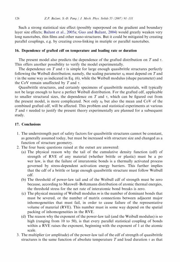
ARTICLE IN PRESSZ.P. Bazant, S.-D. Pang / J. Mech. Phys. Solids 55 (2007) 91–131126
Such a strong statistical size effect (possibly superposed on the gradient and boundarylayer size effects; Bazant et al., 2005a; Guo and Bazant, 2004) would greatly weaken verylong nanotubes, thin films and other nano-structures. But it could be mitigated by creatingparallel couplings, e.g. by creating cross-linking in mutiple or parallel nanotubes.
16. Dependence of grafted cdf on temperature and loading rate or duration
The present model also predicts the dependence of the grafted distribution on T and t.This offers another possibility to verify the model experimentally.The dependence on T and t is simple for large enough quasibrittle structures perfectly
following the Weibull distribution; namely, the scaling parameter s0 must depend on T andt in the same way as indicated in Eq. (6), while the Weibull modulus (shape parameter) andthe CoV remain unaffected by T and t.Quasibrittle structures, and certainly specimens of quasibrittle materials, will typically
not be large enough to have a perfect Weibull distribution. For the grafted cdf, applicableto smaller structural sizes, the dependence on T and t, which can be figured out fromthe present model, is more complicated. Not only s0 but also the mean and CoV of thecombined grafted cdf, will be affected. This problem and statistical experiments at variousT and t needed to justify the present theory experimentally are planned for a subsequentstudy.
17. Conclusions
1.
The understrength part of safety factors for quasibrittle structures cannot be constant,as generally assumed today, but must be increased with structure size and changed as afunction of structure geometry.2.
The four basic questions raised at the outset are answered:(a) The physical reason why the tail of the cumulative density function (cdf) ofstrength of RVE of any material (whether brittle or plastic) must be a power law, is that the failure of interatomic bonds is a thermally activated processgoverned by stress-dependent activation energy barriers. This further impliesthat the cdf of a brittle or large enough quasibrittle structure must follow Weibullcdf.
(b) The threshold of power-law tail and of the Weibull cdf of strength must be zerobecause, according to Maxwell–Boltzmann distribution of atomic thermal energies,the threshold stress for the net rate of interatomic bond breaks is zero.
(c) The physical meaning of Weibull modulus m is the number of dominant bonds thatmust be severed, or the number of matrix connections between adjacent majorinhomogeneities that must fail, in order to cause failure of the representativevolume of material (RVE). This number must in some way depend on the spatialpacking of inhomogeneities in the RVE.
(d) The reason why the exponent of the power-law tail (and the Weibull modulus) is sohigh (ranging from 10 to 50), is that every parallel statistical coupling of bondswithin a RVE raises the exponent, beginning with the exponent of 1 at the atomicscale.
3.
The multiplier (or amplitude) of the power-law tail of the cdf of strength of quasibrittlestructures is the same function of absolute temperature T and load duration t as that
ARTICLE IN PRESSZ.P. Bazant, S.-D. Pang / J. Mech. Phys. Solids 55 (2007) 91–131 127
indicated by Maxwell–Boltzmann distribution for the rate of breaks of interatomicbonds.
4.
The statistical model for RVE can include parallel connections of no more than twoelements on scales close to macroscales (with power-law tail exponent greater thanabout 6), and three elements on lower scales (with power-law tail exponent less thanabout 6), or else the power-law tail of cdf of RVE strength would be so short thatWeibull distribution would never be observed in practice.5.
While the power-law tail exponent of a chain is equal to the lowest exponent among itslinks, the power-law tail exponent of a bundle is equal to the sum of the power-law tailexponents of all the parallel fibers in a bundle, regardless of whether they are brittle orplastic (the same is probably true for softening fibers). While the extent of power-lawtail increases with the length of a chain, it drastically decreases (in cdf scale) with thenumber of fibers in a bundle.6.
A sufficiently long power-law tail of RVE strength can be reconciled with theactivation energy concept only if the RVE is statistically modelled by a hierarchy ofparallel and series couplings, consisting of bundles of sub-chains of sub-bundles of sub-sub-chains of sub-sub-bundles, etc., down to the atomic scale. The Weibull modulus isequal to the minimum number of cuts of elementary bonds needed to separate thehierarchical model into two parts. The elements of the sub-chains and sub-bundles inthe hierarchical model may exhibit plastic or softening behaviors, but not a perfectlybrittle behavior because such behavior would not allow a sufficiently long power-lawtail of the cdf of RVE. The cdf of RVE strength cannot be modelled by a bundle with afinite number of elements following the Maxwell–Boltzmann distribution, andquasibrittle structures cannot be modelled as a chain of bundles. Otherwise, thepower-law tail of RVE would be far too short for generating Weibull cdf for thestrength of large structures.7.
For the sake of engineering computations, the cdf of random strength of a RVE maybe assumed to have Weibull left tail grafted at the failure probability of about0.0001–0.01 onto a Gaussian core. With increasing structure size, the grafting pointmoves to higher failure probabilities as a function of the equivalent number of RVEs,in a way than can be described by treating the structure as a chain of finite RVEs. Themean and CoV of this grafted distribution are easy to calculate and are tabulated.8.
For not too small structures, the present chain-of-RVEs model gives similar results asthe previously developed nonlocal Weibull theory, while for very small structures (notmuch larger than a RVE) it allows predicting failure probability more rationally. Themean behavior is, on not too small scales, essentially equivalent to that of the cohesivecrack model, crack band model and nonlocal damage models.9.
The theory explains why a nonzero threshold was found preferable in previous studiesof coarse-grained ceramics and concrete. The reason is that the strength histograms ofthese materials exhibit a kink separating a lower Weibull segment from an upperGaussian segment. The lower segment up to the kink, important for safe design, can befitted by Weibull cdf with a finite threshold. But the upper segment cannot. The presenttheory removes this problem. The predicted cdf fits both segments of the experimentalhistograms, along with the kink location, very well. This is one experimental verifi-cation of the present theory.10.
Two ways of experimental calibration and verification are proposed. (1) Fit the meansize effect curve, particularly its deviation from the Weibull size effect for small sizes.
ARTICLE IN PRESSZ.P. Bazant, S.-D. Pang / J. Mech. Phys. Solids 55 (2007) 91–131128
(2) Fit the strength histograms with kinks for at least two significantly different sizes(and possibly different shapes). Each way suffices to determine all the parameters. Stillanother check is fitting of experimental strength histograms for different temperatures,loading rates or load durations.
Acknowledgments
Partial financial support under ONR Grant N00014-10-I-0622 and NSF Grant CMS-0556323 (both to Northwestern University), and a Grant from Infrastructure TechnologyInstitute at Northwestern University, is gratefully acknowledged. Thanks for stimulatingdiscussions are due to Martin Z. Bazant, Associate Professor of Mathematics at M.I.T., toDrahomır Novak, Professor at VUT Brno, and to Miroslav Vorechovsky, AssistantProfessor at VUT Brno, Czech Republic.
References
Amar, E., Gauthier, G., Lamon, J., 1989. Reliability analysis of a Si3N4 ceramic piston pin for automotive
engines. In: Tennery, V. (Ed.), Ceramics Materials and Components for Engines. American Ceramic Society,
Westerville, OH, pp. 1334–1346.
Ang, A.H.-S., Tang, W.H., 1984. Probability Concepts in Engineering Planning and Design. vol. II. Decision,
Risk and Reliability. Wiley, New York.
Bansal, G.K., Duckworth, W.H., Niesz, D.E., 1976a. Strength-size relations in ceramic materials: Investigation of
an alumina ceramic. J. Am. Ceram. Soc. 59, 472–478.
Bansal, G.K., Duckworth, W.H., Niesz, D.E., 1976b. Strength analysis of brittle materials. Battelle-Report,
Columbus.
Bartlett, F.M., MacGregor, J.G., 1996. Statistical analysis of the compressive strength of concrete in structures.
ACI Mat. J. 93 (2), 158–168.
Bazant, Z.P., 1984. Size effect in blunt fracture: concrete, rock, metal. J. Eng. Mech. ASCE 110 (4), 518–535.
Bazant, Z.P., 1995. Creep and damage in concrete. In: Skalny, J., Mindess, S. (Eds.), Materials Science of
Concrete IV. American Ceramic Society, Westerville, OH, pp. 355–389.
Bazant, Z.P., 1997. Scaling of quasibrittle fracture: Asymptotic analysis. Int. J. Fract. 83 (1), 19–40.
Bazant, Z.P., 2002. Scaling of Structural Strength (second ed.), Hermes Penton Science (Kogan Page Science),
London, U.K Elsevier, London 2005; French translation, Hermes, Paris 2004.
Bazant, Z.P., 2004a. Probability distribution of energetic-statistical size effect in quasibrittle fracture. Probabilistic
Eng. Mech. 19 (4), 307–319.
Bazant, Z.P., 2004b. Scaling theory for quasibrittle structural failure. Proc. Nat. Acad. Sci. 101 (37), 13397–13399.
Bazant, Z.P., Jirasek, M., 1993. R-curve modeling of rate and size effects in quasibrittle fracture. Int. J. Fract. 62,
355–373.
Bazant, Z.P., Li, Y.-N., 1997. Cohesive crack with rate-dependent opening and viscoelasticity: I. Mathematical
model and scaling. Int. J. Fract. 86 (3), 247–265.
Bazant, Z.P., Novak, D., 2000a. Probabilistic nonlocal theory for quasibrittle fracture initiation and size effect. II.
Application. J. Eng. Mech. ASCE 126 (2), 175–185.
Bazant, Z.P., Novak, D., 2000b. Energetic-statistical size effect in quasibrittle failure at crack initiation. ACI
Mater. J. 97 (3), 381–392.
Bazant, Z.P., Novak, D., 2001. Nonlocal model for size effect in quasibrittle failure based on extreme value
statistics. In: Corotis, R.B. (Ed.), Proceedings of the Eighth International Conference on Structural Safety and
Reliability (ICOSSAR), Newport Beach, CA., 2001, Swets & Zeitinger, Balkema, pp. 1–8.
Bazant, Z.P., Pang, S.D., 2005a. Revision of reliability concepts for quasibrittle structures and size effect on
probability distribution of structural strength. In: Augusti, G., Schueller, G.I., Ciampoli, M., (Eds.),
Proceedings of Ninth International Conference on Structural Safety and Reliability (ICOSSAR), Rome,
Milpress, Rotterdam, pp. 377–386.
ARTICLE IN PRESSZ.P. Bazant, S.-D. Pang / J. Mech. Phys. Solids 55 (2007) 91–131 129
Bazant, Z.P., Pang, S.-D., 2005b. Effect of size on safety factors and strength of quasibrittle structures: Beckoning
reform of reliability concepts. In: Chandra Kishen, J.M., Roy, D. (Eds.), Proceedings of the Structural
Engineering Convention (SEC 2005). Indian Institute of Science, Bangalore, India, pp. 2–20.
Bazant, Z.P., Pang, S.-D., 2006. Mechanics based statistics of failure risk of quasibrittle structures and size effect
on safety factors. Proceedings of the National Academy of Sciences, vol. 103(25), 9434–9439.
Bazant, Z.P., Planas, J., 1998. Fracture and Size Effect in Concrete and Other Quasibrittle Materials. CRC Press,
Boca Raton, FL.
Bazant, Z.P., Prat, P.C., 1988. Effect of temperature and humidity on fracture energy of concrete. ACI Mater. J.
84, 262–271.
Bazant, Z.P., Xi, Y., 1991. Statistical size effect in quasi-brittle structures: II. Nonlocal theory. J. Eng. Mech.
ASCE 117 (17), 2623–2640.
Bazant, Z.P., Yu, Q., 2006. Reliability, brittleness and fringe formulas in concrete design codes. J. Struct. Eng.
ASCE 132(1), 3–12.
Bazant, Z.P., Gu, W.-H., Faber, K.T., 1995. Softening reversal and other effects of a change in loading rate on
fracture of concrete. ACI Mater. J. 92, 3–9.
Bazant, Z.P., Guo, Z., Espinosa, H., Zhu, Y., Peng, B., 2005. Epitaxially influenced boundary layer model for size
effect in thin metallic films. J. Appl. Phys. 97, 073506-1–073506-13.
Bazant, Z.P., Vorechovsky, M., Novak, M., 2005b. Asymptotic prediction of energetic-statistical size effect from
deterministic finite element solutions. J. Eng. Mech. ASCE., in press.
Beremin, F.M., 1983. A local criterion for cleavage fracture of a nuclear pressure vessel steel. Metall. Trans. 114A,
2277–2287.
Bouchaud, J.-P., Potters, M., 2000. Theory of Financial Risks: From Statistical Physics to Risk Management.
Cambridge University Press, Cambridge, UK.
Breysse, D., 1990. A probabilistic formulation of the damage evaluation law. Struct. Saf. 8, 311–325.
Bruhner-Foit, A., Munz, D., 1989. Statistical analysis of flexure strength data. Int. Energy Agency Annex II,
Subtask 4.
Bulmer, M.G., 1967. Principles of Statistics. Dover, New York.
Carmeliet, J., 1994. In: Kusters, G.M.A., Hendriks, M.A.N. (Eds.), On Stochastic Descriptions for Damage
Evolution in Quasi-Brittle Materials. DIANA Computational Mechanics.
Carmeliet, J., Hens, H., 1994. Probabilistic nonlocal damage model for continua with random field properties.
J. Eng. Mech. ASCE 120, 2013–2027.
Chmielewski, T., Konopka, E., 1999. Statistical evaluations of field concrete strength. Mag. Concr. Res. 51 (1),
45–52.
CIRIA, 1977. Rationalization of safety and serviceability factors in structural codes. Construction Industry
Research and Information Association, Report no. 63. London.
Cornell, C.A., 1969. A probability based structural code. ACI J. 66 (12), 974–985.
Cottrell, A.H., 1964. The Mechanical Properties of Matter. Wiley, New York.
Curtin, W.A., Scher, H., 1997. Time-dependent damage evolution and failure in materials. I. Theory. Phys. Rev. B
55 (18), 12038–12050.
Cusatis, G., Bazant, Z.P., Cedolin, L., 2003. Confinement-shear lattice model for concrete damage in tension and
compression: I. Theory. J. Eng. Mech. ASCE 129 (12), 1439–1448.
Daniels, H.E., 1945. The statistical theory of the strength of bundles and threads. Proc. R. Soc. London A 183,
405–435.
Danzer, R., Lube, T., 1996. New fracture statistics for brittle materials. Fract. Mech. Ceram. 11, 425–439.
Duckett, W., 2005. Risk analysis and the acceptable probability of failure. The Struct. Eng. 83 (15), 25–26.
Ellingwood, B.R., McGregor, J.G., Galambos, T.V., Cornell, C.A., 1982. Probability based load criteria: load
factors and load combinations. J. Struct. Eng. ASCE 108 (ST5), 978–997.
Erntroy, H.C., 1960. The variation of works test cubes. Slough, Cement and Concrete Association, Research
Report 10. Publication 41.010, Slough, UK.
Eyring, H., 1936. Viscosity, plasticity and diffusion as examples of absolute reaction rates. J. Chem. Phys. 4, 263.
Eyring, H., Lin, S.H., Lin, S.M., 1980. Basic Chemical Kinetics. Wiley, New York.
Feller, W., 1957. Introduction to Probability Theory and its Applications, second ed. Wiley, New York.
FHWA (Federal Highway Administration) 1998. Concrete strength. Guide to Developing Performance-Related
Specifications for PCC Pavement—Technical Summary. vol. 3, App. C.
Fisher, R.A., Tippett, L.H.C., 1928. Limiting forms of the frequency distribution of the largest and smallest
member of a sample. Proc. Cambridge Philos. Soc. 24, 180–190.
ARTICLE IN PRESSZ.P. Bazant, S.-D. Pang / J. Mech. Phys. Solids 55 (2007) 91–131130
Frantziskonis, G.N., 1998. Stochastic modeling of heterogeneous materials—A process for the analysis and
evaluation of alternative formulations. Mech. Mater. 27, 165–175.
Frechet, M., 1927. Sur la loi de probabilite de l’ ecart maximum. Ann. Soc. Pol. Math. 6, 93–116.
Freudenthal, A.M., 1968. Statistical approach to brittle fracture. In: Liebowitz, H. (Ed.), Fracture: An Advanced
Treatise, vol. 2. Academic Press, New York, pp. 591–619.
Freudenthal, A.M., Garrelts, J.M., Shinozuka, M., 1966. The analysis of structural safety. J. Struct. Div. ASCE
92 (ST1), 619–677.
Gehrke, E., Liebelt, A., Hollstein, T., 1993. Der Zugversuch—Technischer Stand und Perspektive. In: Mechanische
Eigenschaften keramischer Konstruktionswerk-stoffe. DGM Informationsgesellschaft, pp. 291–306.
Glasstone, S., Laidler, K.J., Eyring, H., 1941. The Theory of Rate Processes. McGraw-Hill, New York.
Gumbel, E.J., 1958. Statistics of Extremes. Columbia University Press, New York.
Guo, Z., Bazant, Z.P., 2004. Theoretical modeling and scaling. Section 4, pp. 584–592, 596–600. In: B.C. Prorok,
Y. Zhu, H.D. Espinosa, Z. Guo, Z.P. Bazant, Y. Zhao, B.I. Yakobson (Eds.), Micro- and Nanomechanics,
vol. 5, pp. 555–600. In: H.S. Nalva (Ed.), Encyclopedia of Nanoscience and Nanotechnology, American
Scientific Publishers, Stevenson Ranch, CA.
Gutierrez, M.A., 1999. Objective simulation of failure in heterogeneous softening solids. Dissertation, Delft
University of Technology.
Haldar, A., Mahadevan, S., 2000. Probability, Reliability and Statistical Methods in Engineering Design. Wiley,
New York.
Harlow, D.G., Phoenix, S.L., 1978a. The chain-of-bundles probability model for the strength of fibrous materials.
I. Analysis and conjectures. J. Compos. Mater. 12, 195–214.
Harlow, D.G., Phoenix, S.L., 1978b. The chain-of-bundles probability model for the strength of fibrous materials.
II: A numerical study of convergence. J. Compos. Mater. 12, 314–334.
Harlow, D.G., Smith, R.L., Taylor, H.M., 1983. Lower tail analysis of the distribution of the strength of load-
sharing systems. J. Appl. Probab. 20, 358–367.
Hattori, Y., Tajima, Y., Yabuta, K., Matsuo, J., Kawamura, M., Watanabe, T., 1989. Gas pressure sintered
silicon nitride ceramics for turbocharger applications. In: Tennery, V. (Ed.), Ceramics Materials and
Components for Engines. American Ceramic Society, Westerville, OH, pp. 166–172.
Hill, T.L., 1960. An Introduction to Statistical Mechanics. Addison-Wesley, Reading, MA.
Ito, S., Sakai, S., Ito, M., 1981. Bending strength of hot-pressed silicon nitride. Zairyo 30 (337), 1019–1024.
Jackson, K.E., 1992. Scaling effects in the flexural response and failure of composite beams. AIAA J. 30 (8),
2099–2105.
Julian, O.G., 1955. Discussion of ‘‘Strength variations in ready-mixed concrete’’ by A.E. Cummings. ACI Proc. 51
(12), 772–778.
Katayama, Y., Hattori, Y., 1982. Effects of specimen size on strength of sintered silicon nitride. J. Am. Ceram.
Soc. 65(10), C-164–C-165.
Katz, R.N., Wechsler, G., Toutjanjim, H., Friel, D., Leatherman, G.L., El-Korchi, T., Rafaniello, W., 1993.
Room temperature tensile strength of AIN. Ceram. Eng. Sci. Proc. 14, 282–291.
Koide, H., Akita, H., Tomon, M., 1998. Size effect on flexural resistance due to bending span of concrete beams.
In: Mihashi, H., Rokugo, K. (Eds.), Fracture Mechanics of Concrete Structures, Proceedings of the Third
International Conference on FraMCoS-3 held in Gifu, Japan. Aedificatio Publishers, Freiburg, Germany,
pp. 2121–2130.
Koide, H., Akita, H. and Tomon, M., 2000. Probability model of flexural resistance on different lengths of
concrete beams, in: R.E. Melchers, M.G. Stewart, (Eds.), Application of Statistic and Probability, Proceedings
of the Eighth International Conference, ICASP-8, held in Sydney, Australia, 1999, Balkema, Rotterdam,
vol. 2, pp. 1053–1057.
Lu, C., Danzer, R., Fischer, F.D., 2002a. Fracture statistics of brittle materials: Weibull or normal distribution.
Physical Review E 65, 067102-1–067102-4.
Lu, C., Danzer, R., Fischer, F.D., 2002b. Influence of threshold stress on the estimation of the Weibull statistics.
J. Am. Ceram. Soc. 85 (6), 1640–1642.
Madsen, H.O., Krenk, S., Lind, N.C., 1986. Methods of Structural Safety. Prentice-Hall, Englewood Cliffs, NJ.
Mahesh, S., Phoenix, S.L., Beyerlein, I.J., 2002. Strength distributions and size effects for 2D and 3D composites
with Weibull fibers in an elastic matrix. Int. J. Fract. 115, 41–85.
Matsusue, K., Takahara, K., Hashimoto, R., 1982. Strength evaluation of hot-pressed silicon nitride at room
temperature. Yogyo Kyokai Shi 90 (4), 168.
Mayer, J.E., 1940. Statistical Mechanics. Wiley, New York.
ARTICLE IN PRESSZ.P. Bazant, S.-D. Pang / J. Mech. Phys. Solids 55 (2007) 91–131 131
McCartney, L.N., Smith, R.L., 1983. Statistical theory of the strength of fiber bundles. J. Appl. Mech. 50,
601–608.
McClintock, A.M., Argon, A.S. (Eds.), 1966. Mechanical Behavior of Materials. Addison-Wesley, Reading, MA.
McMeeking, R.M., Hbaieb, K., 1999. Optimal threshold strength of laminar ceramics. Z. Metallk. 90 (12), 1031–1036.
Melchers, R.E., 1987. Structural Reliability, Analysis & Prediction. Wiley, New York.
Metcalf, J.B., 1970. The specification of concrete strength. Part II. The distribution of concrete for structures in
current practice. Crowthorne, Road Research Laboratory. Report LR 300.
Mirza, S.A., Hatzinikolas, M., MacGregor, J.G., 1979. Statistical descriptions of strength of concrete. J. Struct.
Div. ASCE 105 (ST6), 1021–1037.
Neaman, D., Laguros, J.G., 1967. Statistical quality control in Portland cement concrete pavements,
Transportation research record 184, Transportation Research Board, pp. 1–12.
Newman, W.I., Phoenix, S.L., 2001. Time-dependent fiber bundles with local load sharing. Phys. Rev. E 63,
021507-1–012507-20.
NKB (Nordic Committee for Building Structures) 1978. Recommendation for loading and safety regulations for
structural design. NKB Report, no. 36.
Ohji, T., 1988. Towards routine tensile testing. Inter. J. High Technol. Ceram. 4, 211–225.
Phoenix, S.L., 1978. The asymptotic time to failure of a mechanical system of parallel members. SIAM J. Appl.
Math. 34 (2), 227–246.
Phoenix, S.L., 1983. The stochastic strength and fatigue of fiber bundles. Int. J. Fract. 14, 327–344.
Phoenix, S.L., Beyerlein, I.J., 2000. Distribution and size scalings for strength in a one-dimensional random lattice
with load redistribution to nearest and next nearest neighbors. Phys. Rev. E 62 (2), 1622–1645.
Phoenix, S.L., Smith, R.L., 1983. A comparison of probabilistic techniques for the strength of fibrous materials
under local load-sharing among fibers. Int. J. Solids Struct. 19 (6), 479–496.
Phoenix, S.L., Tierney, L.-J., 1983. A statistical model for the time dependent failure of unidirectional composite
materials under local elastic load-sharing among fibers. Eng. Fract. Mech. 18 (1), 193–215.
Phoenix, S.L., Ibnabdeljalil, M., Hui, C.-Y., 1997. Size effects in the distribution for strength of brittle matrix
fibrous composites. Int. J. Solids Struct. 34 (5), 545–568.
Quinn, G.D., 1990. Flexure strength of advanced structural ceramics, a round robin. J. Am. Ceram. Soc. 73 (8),
2374–2384.
Quinn, G.D., Morrell, R., 1991. Design data for engineering ceramics: a review of the flexure test. J. Am. Ceram.
Soc. 74 (9), 2037–2066.
Rao, M.P., Sanchez-Herencia, A.J., Beltz, G.E., McMeeking, R.M., Lange, F.F., 1999. Laminar ceramics that
exhibit a threshold strength. Science 286, 102–104.
Rusch, H., Sell, R., Rackwitz, R., 1969. Statistical analysis of concrete strength. Deutscher Ausschuss Stahlbeton
Heft 206.
Santos, C., Strecker, K., Neto, F.P., Silva, O.M.M., Baldacim, S.A., Silva, C.R.M., 2003. Evaluation of the
reliability of Si3N4–Al2O3–CTR2O3 ceramics through Weibull analysis. Mater. Res. 6 (4), 463–467.
Sato, S., Taguchi, K., Adachi, R., Nakatani, M., 1996. A study on strength characteristics of Si3N4 coil springs.
Fatigue Fract. Eng. Mater. Struct. 19 (5), 529–537.
Shalon, R., Reintz, R.C., 1955. Interpretation of strengths distribution as a factor in quality control of concrete.
Proc. Reunion Int. des Lab. d’Essais et de Recherches sur les Materiaux et les Constr., Symp on the
Observation of Sub-struct., vol. 2, Laboratorio Naciano de Engenharia Civil, Lisbon, Portugal, pp. 100–116.
Smith, R.L., 1982. The asymptotic distribution of the strength of a series-parallel system with equal load sharing.
Ann. Probab. 10 (1), 137–171.
Smith, R.L., Phoenix, S.L., 1981. Asymptotic distributions for the failure of fibrous materials under series-parallel
structure and equal load-sharing. J. Appl. Mech. 48, 75–81.
Soma, T., Matsui, M., Oda, I., 1985. Tensile strength of a sintered silicon nitride. In: Proceedings of Non-oxide
Technical and Engineering Ceramics, Limerick, Ireland. July 10–12 1985, pp. 361–374.
Soong, T.T., 2004. Fundamentals of Probability and Statistics for Engineers. Wiley, New York.
Tobolsky, A.V., 1960. Structure and Properties of Polymers. Wiley, New York.
Weibull, W., 1939. The phenomenon of rupture in solids. Proceedings of Royal Swedish Institute of Engineering
Research vol. 151, Stockholm, pp. 1–45.
Weibull, W., 1951. A statistical distribution function of wide applicability. J. Appl. Mech. ASME 153 (18), 293–297.
Zhurkov, S.N., 1965. Kinetic concept of the strength of solids. Int. J. Fract. Mech. 1 (4), 311–323.
Zhurkov, S.N., Korsukov, V.E., 1974. Atomic mechanism of fracture of solid polymers. J. Polym. Sci. 12 (2),
385–398.

![EXTREME PROGRAMMINGfse.studenttheses.ub.rug.nl/8856/1/Infor_Ma_2001_TdeJong.CV.pdf · EXTREME PROGRAMMING 3.1. WHAT IS EXTREME PROGRAMMING? According to vd)sitc [3], Extreme Programming](https://img.pdfslide.net/doc/110x75/6008914c858cab1a066c00ad/extreme-extreme-programming-31-what-is-extreme-programming-according-to-vdsitc.jpg)