Embed Size (px)
Citation preview
Active Dynamic Analysis and Vibration Control of Gossamer Structures Using Smart Materials
Eric J. Ruggiero
Thesis submitted to the Faculty of the
Virginia Polytechnic Institute and State University
in partial fulfillment of the degree requirements for the degree of
Master of Science
in
Mechanical Engineering
Daniel J. Inman, chair
Harry Robertshaw
Donald Leo
Walter F. OBrien
May 7, 2002
Blacksburg, Virginia
Keywords: Inflatable structures, piezoelectric, modal, PPF control,
MIMO, gossamer spacecraft
Copyright 2002, Eric J. Ruggiero

Active Dynamic Analysis and Vibration Control of Gossamer Structures Using
Smart Materials
Eric J. Ruggiero
(Abstract)
Increasing costs for space shuttle missions translate to smaller, lighter, and more
flexible satellites that maintain or improve current dynamic requirements. This is
especially true for optical systems and surfaces. Lightweight, inflatable structures,
otherwise known as gossamer structures, are smaller, lighter, and more flexible than
current satellite technology. Unfortunately, little research has been performed
investigating cost effective and feasible methods of dynamic analysis and control of these
structures due to their inherent, non-linear dynamic properties. Gossamer spacecraft have
the potential of introducing lenses and membrane arrays in orbit on the order of 25 m in
diameter. With such huge structures in space, imaging resolution and communication
transmissibility will correspondingly increase in orders of magnitude.
A daunting problem facing gossamer spacecraft is their highly flexible nature.
Previous attempts at ground testing have produced only localized deformation of the
structures skin rather than excitation of the global (entire structures) modes.
Unfortunately, the global modes are necessary for model parameter verification. The
motivation of this research is to find an effective and repeatable methodology for
obtaining the dynamic response characteristics of a flexible, inflatable structure. By
obtaining the dynamic response characteristics, a suitable control technique may be
developed to effectively control the structures vibration. Smart materials can be used for
both active dynamic analysis as well as active control. In particular, piezoelectric
materials, which demonstrate electro-mechanical coupling, are able to sense vibration and
consequently can be integrated into a control scheme to reduce such vibration. Using
smart materials to develop a vibration analysis and control algorithm for a gossamer
space structure will fulfill the current requirements of space satellite systems. Smart
materials will help spawn the next generation of space satellite technology.

iii
Grant Information
This work was sponsored by the Air Force Office of Scientific Research under
grant number F49620-99-1-0231, by the NASA Langley Research Center under grant
number LaRC 01-1103, and by the Honeywell Corporation. The author gratefully
acknowledges the support.

iv
for my wife, Jennifer

v
Acknowledgements
I am quite thankful to a lot of people in seeing the successful completion of this
work. First, I would like to thank God for the endless blessings and gifts He has
bestowed upon me. Without His love, comfort, and guidance, not to mention answered
prayers, I would never have made it to this point in my life.
I am in deep gratitude for the guidance and support of my academic advisor, Dr.
Daniel J. Inman. Dr. Inman took me under his wing last fall and provided me with a
thesis topic and the funds to see its fruition. His thoughtful and insightful feedback
throughout the semesters continued to challenge my work and bring it to higher levels. I
also extend a heartfelt thanks to Dr. Gyuhae Park. Dr. Park worked hand-in-hand with
me in the laboratory and helped me maintain some form of sanity throughout endless
experimental problems. Without his help, Id still be trying to figure out the dynamic
analysis portion of this research.
I was blessed with support of my thesis throughout both semesters by many
others. Dr. Jan Wright, from the University of Manchester in the U.K., provided a huge
boost to my thesis by working with me on the development of MIMO testing techniques
and processing software in the dynamic analysis of gossamer structures. Drs. Donald
Leo and Harry Robertshaw helped shed some light on my thesis work when I needed it
most, especially from the controls engineering side.
Friendships formed at Virginia Tech have also helped keep me sane during some
of the most trying times of my academic work. I extend my thanks to Mark, Chuck, Ean,
Noah, Luciano, Kevin, Rodrigo, Curt, Akhilesh, Nikola, and everyone else who has ever
been there for me.

vi
Acknowledgements (cont.)
I also need to thank two of the most important people in the world, my parents.
Without their love and financial support throughout my undergraduate career, I would not
have had the opportunity to continue my education. I learned motivation, dedication, and
the pursuit of excellence from their guidance and example. Thank you, Mom and Dad,
and my entire family.
Last but certainly not least, I am most indebted to my wife, Jennifer. Jennifer has
fully supported my education and pursuit of higher learning while delaying some of her
own life goals and dreams. She has been there for me on my best days as well as my
worst days, and has always offered wisdom to keep me focused on what is important in
lifefamily and prayer. Without Jennifer, I could not have finished this thesis in two
semesters. Her love and passion are the drive behind my success. Thank you, Jennifer,
from the bottom of my heart.

vii
TABLE OF CONTENTS
Page
CHAPTER I: INTRODUCTION 1
1.1 Background 1
1.2 Motivation.. 2
1.3 Research Objectives and Contributions. 3
1.4 Thesis Outline 4
CHAPTER 2: LITERATURE REVIEW 6
2.1 Introduction... 6
2.2 The Importance of Gossamer Spacecraft Technology.. 6
2.3 Historical Perspective 8
2.4 A History of Experimental Modal Analysis Work
on Gossamer Craft... 12
2.4.1 Experimental Modal Analysis of Tires 12
2.4.2 Experimental Modal Analysis of Gossamer Spacecraft
and an Inflated Torus.. 14
2.4.3 Use of Smart Materials in the Modal Analysis
of Gossamer Spacecraft.. 17
2.5 The Future of Gossamer Spacecraft Technology. 21
CHAPTER 3: DYNAMIC ANALYSIS OF AN INFLATABLE TORUS
USING SMART MATERIALS. 23
3.1 Background. 23
3.2 Experimental Modal Analysis of an Inflated Torus Using
Traditional Excitation Methods.. 24
3.2.1 Test Structure: A Kapton Torus 24
3.2.2 Excitation.. 25
3.2.3 Sensors.. 26
3.2.4 Experimental Procedure.... 27

viii
3.2.5 Results and Analysis.. 27
3.3 Macro-fiber Composite Actuation of an Inflated Structure 35
3.3.1 Experimental Configuration of the MFC® Actuator.. 36
3.3.2 Results and Analysis.. 37
3.4 The Limitations of SISO Experimentation.. 42
3.5 Chapter Summary 43
CHAPTER 4: MULTI-INPUT MULTI-OUTPUT EXPERIMENTAL
MODAL ANALYSIS OF AN INFLATED TORUS. 45
4.1 Background.. 45
4.2 MIMO Theoretical Development. 45
4.3 The MIMO Experiment 48
4.3.1 Linearity Check... 49
4.3.2 MIMO Experimental Results.. 50
4.3.3 Post-Processing the Results. 54
4.4 Chapter Summary. 55
CHAPTER 5: POSITIVE POSITION FEEDBACK CONTROL OF A PLATE
USING AN MFC® SENSOR.. 57
5.1 Introduction.. 57
5.2 Background on Positive Position Feedback Control Theory and
Implementation. 57
5.3 Dynamic Analysis of a Simply Supported Plate... 60
5.3.1 Analytical Solution to the Simply Supported Plate
Vibration Problem 60
5.3.2 Experimental Modal Analysis of the Simply Supported
Plate.. 62
5.4 Vibration Control of a Simply Supported Plate Using a
PPF Controller.. 66
5.5 Chapter Summary.. 72

ix
CHAPTER 6: COMPARISON BETWEEN ACTIVE AND PASSIVE
CONTROL TECHNIQUES FOR AN INFLATABLE TORUS. 73
6.1 Background... 73
6.2 Active Control of the Gossamer Torus Using a PPF Controller... 73
6.3 Passive Control of the Gossamer Torus Using Viscoelastic Tape 77
6.4 Comparison Between Active and Passive Methods of Vibration
Control for the Torus. 79
6.5 Chapter Summary.. 80
CHAPTER 7: CONCLUSIONS AND FUTURE WORK.. 81
APPENDIX A: MATLab Code 86
APPENDIX B: 3M Damping Foil (2552) Data Sheets 109
APPENDIX C: MFC® Device Properties. 112
REFERENCES. 113
VITA. 118

x
LIST OF FIGURES
Figure Page
2.1: NASAs Inflatable Antenna Experiment (IAE) fully deployed in orbit... 9
2.2: A timeline showing the years of industrial research contributed to the
growth of gossamer technology. 11
3.1: The Kapton torus under experimental investigation. 25
3.2: Electromagnetic shaker attachment to the skin of the torus.. 26
3.3: PVDF sensor attached to the skin of the inflated torus. 26
3.4: A sample curve-fitted FRF from the collected modal data using the UMPA
pseudo least squares method. 28
3.5: Out-of-plane FRF curve and coherence plot, electromagnetic shaker
excitation 30
3.6: In-plane FRF curve and coherence plot, electromagnetic shaker excitation. 31
3.7: Out-of-plane and in-plane mode shapes identified using an accelerometer
as a sensor.. 33
3.8: Out-of-plane and in-plane mode shapes identified using a PVDF sensor. 34
3.9: MFC® actuator attached to the skin of the torus with double-sided tape.. 36
3.10: Sample FRF curve and coherence plot using the MFC® actuator as an
excitation source (10-100 Hz range) 38
3.11: Sample FRF curve and coherence plot using the MFC® actuator as an
excitation source (10-200 Hz range) 39
3.12: Identified out-of-plane mode shapes using the MFC® actuator as an
excitation source (10-200 Hz range) 41
3.13: Orthogonal mode pair of an axi-symmetric torus 43
4.1: SISO tests to estimate FRF curves 46
4.2: MIMO tests to estimate FRF curves. 46
4.3: Experimental setup with multiple sensors and actuators.. 48
4.4: Linearity check FRF results from the torus.. 49
4.5: Sample MIMO FRF curve and coherence function.. 51
4.6: H11 and H21 FRF comparison between SISO and MIMO testing methods... 52

xi
Figure Page
4.7: H12 and H22 FRF comparison between SISO and MIMO testing methods... 53
4.8: Output plot of the polyreference function program... 54
5.1: A block diagram of a PPF controller. 58
5.2: Orthographic views of the simply supported steel plate 60
5.3: The simply-supported test plate under investigation. 62
5.4: The PZT patch location designations assigned to the experiment. 63
5.5: Diagram of the experimental setup for the test plate under dynamic analysis.. 63
5.6: Charge amplifier circuit used to amplify the output of the MFC sensor... 64
5.7: Photograph of the actual charge amplifier used through the experiment.. 64
5.8: FRF of the test plate (accelerometer and MFC sensor comparison). 65
5.9: Diagram of the PPF control experimental setup 68
5.10: SIMULINK block diagram used to implement to the PPF controller. 69
5.11: The first mode of the plate is reduced by 80% using a PPF controller... 70
5.12: Real time response of the plate and control voltage with PPF controller
turned on.. 71
6.1: The active PPF controller experimental setup... 74
6.2: Schematic diagram of the experimental setup to actively control the
gossamer torus... 75
6.3: The PPF controller reduces the magnitude of the first mode of vibration
by 70%... 76
6.4: The vibratory response of the torus and control voltage of the PPF filter. 77
6.5: Passive vibration control experimental setup 78
6.6: The effect of applying viscoelastic tape on the skin of the torus has
negligible effect of the torus.. 79

xii
LIST OF TABLES
Table Page
2.1: Synopsis of recent and future gossamer spacecraft missions as
outlined by NASA. 22
3.1: Summary of the physical properties of the Kapton® torus 25
3.2: Summary of the out-of-plane and in-plane natural frequencies of the torus. 35
3.3: Identified in-plane and out-of-plane resonant frequencies of the torus
with MFC® actuation. 42
4.1: Comparison between SISO and MIMO identified natural frequencies of
the torus. 55
5.1: Summary of the physical properties of the cold-rolled steel plate 61
5.2: The first three natural frequencies of the plate.. 61
5.3: Comparison between the analytically and experimentally determined
resonant frequencies of the plate66
1
CHAPTER 1: Introduction 1.1 Background Lightweight, inflatable space structures are the future of space satellite
technology. Possessing ideal space launching characteristics, such as minimal storage
volume and minimal mass, these lightweight, inflatable structures will propel the space
industry into the next generation of space satellite technology. However, there are
certain, key issues that must be investigated before such structures can replace current
satellite technology. In particular, the vibration characteristics of thin, flexible, and
inflatable structures must be well understood. Space satellites must be expertly
controlled from a vibration standpoint because signal transmission to and from the earth
mandates tight tolerances. Vibration control is critical to mission success as well as
satellite longevity.
Lightweight, inflatable structures possess unique characteristics that make them
difficult candidates for vibration analysis and control. Because these structures are
inflated, issues such as inflation pressure, pressure distribution, and skin wrinkling hurdle
into the forefront of the vibration analysts mind. In terms of space applications, inflated
structures would undergo severe environmental changes as the satellite passed from
orbital day to orbital eclipse. Such environmental changes subject the inflated satellite to
pressure fluctuations and consequent shockwaves that vibrate the structure. Further, such
satellites are susceptible to vibration while in orbit because of local disturbances or rigid
body motion during satellite repositioning. Therefore, the vibration analysis and control
for an inflated structure must be robust in order to handle multitudes of vibration sources,
and must also conform to the lightweight, flexible nature of the structure. For the first
time in current literature, the use of smart materials is proposed as the solution to the
vibration analysis and control of a flexible toroidal structure.
Smart materials, or more specifically, piezoelectric materials, are a viable,
immediate solution to the robust vibration control problem because of their unobtrusive
2
nature and ability to be fully integrated into any control scheme. Lead zirconate titanates
(PZTs) and polyvinylidene fluorides (PVDFs), are two particular types of smart
materials. In the piezoelectric family of materials, if the material is strained it produces
an electric charge and, conversely, if an electric field is applied, the material strains. This
property, known as the piezoelectric effect, has been developed over the past few decades
for use in vibration control schemes of reliable aluminum truss-and-beam technology, as
well as a myriad of other design schemes. In the past decade, significant improvements
have been made in the versatility of these piezoelectric materials. Where standard PZT
ceramics are hard and brittle, piezoelectric polymers (such as PVDF) and macro-fiber
composite (MFC) actuators are pliable, flexible, and readily available. PVDF sensors
and MFC actuators are able to conform to doubly curved surfaces, which brings inflatable
structure technology back into the picture. If these PVDF and MFC patches can be fully
integrated into the skin or onto the surface of an inflatable satellite, then we can measure
the frequency response and implement a control scheme to control the vibration of the
structure.
1.2 Motivation
Increasing costs for space shuttle missions translate to smaller, lighter, and more
flexible satellites that maintain or improve current dynamic requirements. This is
especially true for optical systems and surfaces. Lightweight, inflatable structures, due to
their unique physical characteristics, are smaller, lighter, and more flexible than current
satellite technology. Unfortunately, little research has been performed investigating cost
effective and feasible methods of dynamic analysis and control of these structures due to
their inherent non-linear dynamic properties. Current attempts at ground tests have been
difficult because of the unique nature of the inflated structure and the consequent
difficulties in sensing and actuation. The extremely flexible nature of the structure
produces only localized deformation of the skin rather than excitation of the global
modes. Unfortunately, the global modes are necessary for model parameter verification.
The motivation of this research is to find an effective and repeatable methodology for
obtaining the dynamic response characteristics of a flexible, inflatable structure. By
3
obtaining the dynamic response characteristics of the structure, a suitable control
technique may be developed to effectively control the structures vibration. Developing a
vibration analysis and control algorithm for an inflatable space structure will fulfill the
current requirements of space satellite systems, and will help spawn the next generation
of space satellite technology.
1.3 Research Objectives and Contributions
There are three main objectives of this research: 1) obtaining an accurate dynamic
analysis of a flexible, inflated toroidal structure; 2) establish an effective control scheme
to suppress the vibration of a flexible, inflated toroidal structure; and 3) comparing and
contrasting active and passive vibration control techniques of a flexible, inflated toroidal
structure.
The first objective is developing a methodology using smart materials to obtain an
accurate dynamic analysis of an inflatable satellite system. An accurate dynamic analysis
of a test structure requires a sensor and an actuator to generate a frequency response
function. Polyvinylidene fluoride (PVDF), one type of piezoelectric material, is an ideal
sensor candidate for the dynamic analysis of flexible, inflatable structures. PVDF sensors
conform to any surface, including the doubly curved surface of a toroidal structure, and
can be fully integrated into the skin of a torus or any inflatable structure. Similarly,
macro-fiber composite (MFC) actuators, produced by NASA Langley Research Center,
are ideal candidates for providing input energy to inflatable structures. The thin, flexible
MFC patch is also able to conform to most surfaces, including the doubly curved surface
of an inflatable torus. By implementing an MFC patch to excite a torus, the rigid body
modes of the structure, as well as the point deformation difficulties associated with more
traditional modal testing techniques, can be avoided. Using both PVDF and MFC
patches, an accurate frequency response function can be generated. Throughout
experimentation, the results of the PVDF / MFC combination were compared to the
results of the more conventional accelerometer / electromagnetic shaker combination. As
an extension of this research, the ability to use multiple sensors and multiple actuators to
4
perform a multi input, multi output (MIMO) experimental modal analysis of the torus is
also explored.
Secondly, the aim of this research is to actively control the vibration of a flexible,
inflated toroidal structure using smart materials. Again, the MFC actuator is an ideal
candidate for the active suppression of an inflated structures vibration. In accordance
with current literature, a positive position feedback (PPF) control methodology is used to
effectively control the first resonant frequency of the torus. The active vibration
suppression procedure is first validated on the first mode of vibration of a simply
supported steel plate. Following the success of the plate experiment, the same
experimental configurations are used on the inflated torus. Finally, the research evaluates
the effectiveness of a viscoelastic tape as a passive control technique and compares the
results to that of the active PPF controller.
1.4 Thesis Outline
The research comprising this thesis will be presented in the same order as the
research objectives previously discussed. The second chapter is a literature review
encompassing most of the history of gossamer technology. The third chapter presents the
experimental setup and results of using PVDF film as sensors and MFC actuators as
system excitation sources to obtain the frequency response function of a flexible, inflated
torus. The results are compared to conventional accelerometer / electromagnetic shaker
FRF generation techniques. The fourth chapter of this thesis work will delve into multi
input, multi output experimental modal analysis techniques for a gossamer structure like
the inflated torus. The fifth chapter discusses the experimental setup of a simply
supported plate actively controlled by an MFC sensor / PZT patch actuator combination
and a positive position feedback control algorithm. Using these results as a transition,
chapter six explains the experimental setup of the same control techniques as used on the
simply supported plate, but applied to the inflated torus. Similarly, a passive damping
vibration control experiment will also be performed on the torus using a viscoelastic tape
(3M damping foil #2552), and the results of both the active and passive techniques are

5
compared and contrasted. The final chapter, chapter seven, summarizes the important
conclusions of the research and makes recommendations for future work.
6
CHAPTER 2: Literature Review
2.1 Introduction
On August 12, 1960, NASA successfully launched the first communications
satellite into space. Echo I, a 100-foot diameter hollow ball of aluminum, was the
pioneer of inflatable space satellite technology. However, because of uncertainties in
meteoroid flux and difficulties in manufacturing and controllability, inflatable satellite
technology nearly vanished soon after the satellite launches of the 1960s. Instead, NASA
concentrated on using aluminum truss and beam elements in its satellite design.
Although it has been over forty years since Echo Is successful deployment into Earths
atmosphere, significant advances in materials, or in particular, piezoelectric materials,
have reopened the possibility to using inflatable satellite technology (Chmielewski et al.,
2000).
Since the 1960s, gossamer spacecraft technology has, inherent to its name, floated
through the scientific community like wisps of cobweb caught in the wind. Tenuous and
nearly invisible, gossamer technology has always looked good on paper but, practically
speaking, been difficult to implement. Recent efforts by NASA, the Air Force, and
industry (in particular, LGarde, Inc.) have spun their own nets in the wind to catch wisps
of gossamer technology. Their combined efforts are collectively trying to make the
dreams of yesterday become the realities of today. Having found a niche, research
efforts in many disciplines are now focusing their resources on exploiting the feasibility
and manifestation of gossamer spacecraft and structures.
2.2 The Importance of Gossamer Spacecraft Technology
In engineering terms, gossamer spacecraft are any such space-inflated craft
exhibiting two distinct traits: ultra-low-mass and minimal stowage volume. A space

7
inflatable structure is, according to Artur Chmielewski, a specific application of a
membrane structure or any ultra-low-mass hybrid structure with an extensive use of
membranes. [They are] structures (load-carrying artifacts or devices) comprised of
highly flexible (compliant) plate or shell-like elements (2000). The benefits of using
such structures boil down to the age-old idiom that, in terms of space mission
capabilities, size does matter.
Current restrictions in space satellite technology are governed by the size of the
orbiter. The larger the structure, the larger the lens, aperture, or array contained within it.
By increasing the diameter of these particular components, the satellites imaging
resolution, frequency bandwidth, and sensing capabilities will correspondingly increase.
Unfortunately, such satellite dimensions are infeasible with traditional composite beam
and truss technology. Such structures are limited in size and mass because of the size of
the Space Shuttle cargo bay as well as the high cost associated with each kilogram of
mass launched into orbit. Gossamer craft are the next logical step in the progression of
satellite design and construction. Their ultra-low mass and membrane construction, as
described by Chmielewski (2000), make them the ideal candidates for future satellite
missions. Not only will gossamer craft be able to meet the scientific communitys goals
of super-large craft in outer space, they will also answer the taxpayers concerns over
increasing mission costs.
When looking at the building blocks of gossamer satellites, there are three main
components: inflatable struts, an inflatable torus, and some sort of lens, aperture, or array
housed inside the boundary of the torus. Although all three components interact
dynamically as well as statically, the key, central component is the torus. The torus
serves as the boundary condition for any housed membrane or lens, and it ties together
the supporting struts of the satellite or craft. Therefore, the torus will serve as the
cornerstone of the papers reviewed in this chapter.
In general, the purpose of this chapter is to explore the history of gossamer
spacecraft literature from an experimental standpoint. As in all engineering systems,
8
there is an underlying truth that the engineer must uncover, learn from, and develop. For
gossamer spacecraft, the uncovering of this underlying truth begins with a strong
understanding of the mathematical relationships governing the dynamic behavior of an
inflated torus. This chapter will concentrate on the experimental results published thus
far in the literature, ranging from initial tire experiments to state-of-the-art modal
analyses of a scaled-model gossamer spacecraft component.
2.3 Historical Perspective
In History of Relevant Inflatable High-Precision Space Structures Technology
Developments, author R. F. Freeland (2000) beautifully outlines the history of
deployable space structures. The origins of inflatable structure technology date back to
the late 1950s to mid-1960s, during which time Goodyear Corporation developed ideas
of inflatable structures for its search radar antenna, radar calibration sphere, and
lenticular inflatable parabolic reflector (Freeland, 2000). Each of these three projects
contributed significantly to the overall gossamer structure effort. The inflatable search
radar antenna used rigidizable truss members and a metallic mesh to form the surface of
the aperture. From the project, developed concepts included: the fabrication, assembly,
and alignment of inflatable elements; techniques for attaching inflatable support members
to precision mesh surfaces; and deployment techniques for a complex, inflatable
structure. The radar calibration sphere, 6-meters in diameter, was constructed from
multiple hexagonal-shaped membrane panels. It contributed to gossamer spacecraft by
demonstrating: thin-film processes; high-precision panel assembly; inflation of a large,
thin-film structure; and metalization of thin-film (for high RF reflectivity). Finally,
Goodyear Corporations lenticular inflatable parabolic reflector consisted of a reflector
supported by a torus. From the experimental work, innovations in inflatable structure
production and attainable precision on a much larger scale were realized.
Concurrently with Goodyear Corporations work, NASA Langley Research
Center and NASA Goddard Space Center were developing the first passive space-based
9
communication reflector, Echo I. On August 12, 1960, a Delta rocket deployed the Echo
I communications sphere at an altitude of 1610 km (or 1000 miles).
Freeland also states that after Echo Is successful deployment, emphasis was
placed on very large baseline interferometry (VLBI) axisymmetric reflector antennas,
offset reflectors, and sunshade supports for large sensors and telescopes. During the
development of these technologies in the early 1970s through the late 1980s, a small
private firm known as LGarde, Inc. entered the gossamer technology picture and
contributed significantly to these three main efforts. LGarde Inc.s technological
achievements throughout the 70s and 80s led to the NASA sponsored IN-STEP
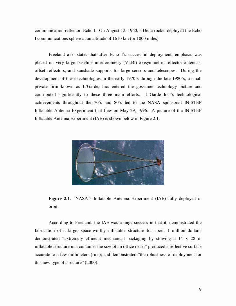
Inflatable Antenna Experiment that flew on May 29, 1996. A picture of the IN-STEP
Inflatable Antenna Experiment (IAE) is shown below in Figure 2.1.
Figure 2.1. NASAs Inflatable Antenna Experiment (IAE) fully deployed in
orbit.
According to Freeland, the IAE was a huge success in that it: demonstrated the
fabrication of a large, space-worthy inflatable structure for about 1 million dollars;
demonstrated extremely efficient mechanical packaging by stowing a 14 x 28 m
inflatable structure in a container the size of an office desk; produced a reflective surface
accurate to a few millimeters (rms); and demonstrated the robustness of deployment for
this new type of structure (2000).

10
Freeland also mentions the contributions of other companies within industry to
the gossamer technology initiative, as quoted below:
1) SRS Technologies (ultra thin film rib).
2) Winzen Engineering, Inc. (large-scale inflatable manufacturing).
3) Sigma Labs, Inc. (ultrahigh barrier films).
4) ITN Energy Systems, Inc. (reversible rigidizable structures).
5) Vertigo, Inc. (inflatable toroidal structures).
6) Millimeter Wave Technology, Inc. (spherical fresnel polymer reflectors).
7) United Applied Technologies, Inc. (precision film structures).
8) Adherent Technologies, Inc. (advanced materials).
9) Energen, Inc. (rigidized membrane reflectors).
10) [ILC Dover (large solar arrays and efficient packaging techniques)].
A timeline emphasizing the major contributions to gossamer technology is shown
in Figure 2.2.
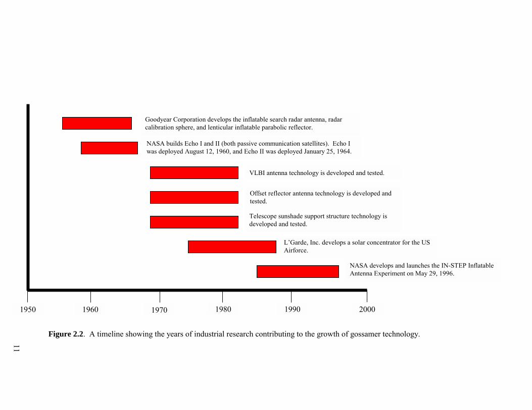
11
Figure 2.2. A timeline showing the years of industrial research contributing to the growth of gossamer technology.
1950 1960 1970 1980 1990 2000
Goodyear Corporation develops the inflatable search radar antenna, radar calibration sphere, and lenticular inflatable parabolic reflector.
NASA builds Echo I and II (both passive communication satellites). Echo I was deployed August 12, 1960, and Echo II was deployed January 25, 1964.
VLBI antenna technology is developed and tested.
Offset reflector antenna technology is developed and tested.
Telescope sunshade support structure technology is developed and tested.
LGarde, Inc. develops a solar concentrator for the US Airforce.
NASA develops and launches the IN-STEP Inflatable Antenna Experiment on May 29, 1996.
12
2.4 A History of Experimental Modal Analysis Work on Gossamer Craft
The following section is dedicated to the work of many experimentalists in the
field of gossamer technology. It is the compilation of these researchers results and
thoughts that has laid the track for future gossamer spacecraft projects. This section will
review the historical development of experimental techniques and modal analyses of
inflatable toroidal structures.
2.4.1 Experimental Modal Analysis of Tires
Although tires are a slightly older concept compared to gossamer spacecraft
technology, they must be briefly addressed since they provide the foundation for this
investigation. The research efforts of only a few will be presented to give but a short
synopsis of some of the developments in this field. The equations governing the
dynamics of an inflated tire differ from that of a gossamer toroidal structure. However,
understanding the development of modal analysis methodologies for tires will prove
fruitful in developing the same applications for inflated tori.
In 1973, Clark et al. performed research investigating the dynamic properties of
aircraft tires. Using what they referred to as string theory, they predicted the behavior
of aircraft tires that shimmy during taxiing. To validate the theoretical results, the group
built a series of scale models representing different aircraft tires. Although the magnitude
of their predictions were not accurate, the relative trends and phase agreement in their
developed transfer functions were surprisingly good.
Noor and Tanner (1985) published a paper surveying the current advances in
finite element modeling and computational algorithms for tire dynamic analysis. Their
survey provides an excellent review of different methods of finite element analysis,
highlighting important issues like material properties, loading scenarios, and tire
construction techniques. At this point in history, however, the authors realized that
13
current experimental validation techniques were inadequate, especially in determining the
dynamic response of the inflated torus.
Fast forward yet another decade, and enter the research efforts of Guan et al.
(2000). In 2000, the authors presented a new method of experimental modal analysis for
inflated tires. Although experimental modal analysis had been performed on tires in the
early sixties through the late eighties, a clear methodology had not been established. The
authors investigated the best methods of tire suspension, excitation type, and device for
excitation. In terms of suspension, the authors found that by hanging the tire from a long,
elastic line, they were able to reduce the rigid body modes to 1-2 Hz, well out of the
frequency range of interest of their experiments. Arguably the authors most important
contribution to this area of research was their investigation of excitation sources. Guan et
al. acquired their frequency response functions using a sine sweep, but the time length
of the excitation signal was carefully selected so that the excitation ceased and that the
corresponding response signal in a data frame was damped out. In this manner, not only
could the leakage problem be solved, but also the reduction of resolution and the
overestimation of damping due to the windowing technique was avoided (2000). Their
specified excitation source is seen throughout some of the most cutting edge modal
analysis research efforts in gossamer technology. Finally, the authors also noted that
point excitation sources were the best input-energy mechanisms for the tire modal
analysis as opposed to a platform-based method. Their research efforts provided key
modal parameters, such as damping, resonant frequencies, and effects of increased
inflation pressure on these properties.
Concurrently with Guan et al., Yam et al. (2000) also performed modal analyses
on tires. In particular, though, the authors research efforts were focused on radial
excitation methods as well as tangential excitation methods in order to develop accurate,
three-dimensional mode shapes of the tire. The efforts of Yam et al. and Guan et al.
helped establish consistent and accurate experimental modal analysis methodologies for
inflated tires.
14
2.4.2 Experimental Modal Analysis of Gossamer Spacecraft and an Inflated Torus
While efforts were being made to identify system parameters of automotive and
aircraft tires, similar efforts began to take shape for gossamer spacecraft. However,
where the difficulty in modeling an automotive or aircraft tire is how to simulate real
working conditions throughout the experimentation, pioneers in system modeling for
gossamer craft faced many additional uncertainties. For example, the harsh environment
of space, meteoroid flux, and vacuum conditions are difficult phenomena to model on
earth. Further, the inflatable structures inherently contain properties that make modal
analyses difficult. Their highly flexible nature, dependency on internal pressure, non-
linear skin wrinkling, and susceptibility to local deformation have challenged the
gossamer technology field since the launching of Echo I. The following is a review of the
work performed by many modal experimentalists on multiple gossamer spacecraft
designs.
In 1998, Tinker performed research at the NASA/Marshall Space Flight Center on
the Shooting Star Experiment (SSE). The SSE was conceived to technologically
demonstrate the possibility of solar thermal propulsion. In brief, solar thermal propulsion
is obtained by concentrating solar energy (sunlight) into a thermal storage engine. Once
heated to a specified level, a propellant is injected into the storage engine and then
expands through a rear nozzle to produce thrust. Since only a few newtons of force are
produced, the craft must be lightweight. Hence, the body of the SSE consists of a
Kapton torus and three Kapton struts. All three pieces are inflated once the experiment
has been placed in orbit. The torus holds the solar concentrator, a parabolic membrane.
Tinker performed a series of analyses on the SSE in both ambient and vacuum
conditions, and analyzed both the inflated struts of the assembly and the concentrator as
two separate modal tests. The modal tests were performed using an electromagnetic
shaker; however, Tinker was unable to directly excite the structure and therefore applied
the input energy to the support plate of the entire assembly. In summary, the inflated
struts were observed to behave like beams in a free-free boundary condition, and their
15
natural frequencies changed as a function of both the film thickness and pressure inside
the structure (1998). Modal tests were performed on the entire assembly at pressures of
0.25, 0.5, and 1.0 psig. It is also noted that 0.5 psig is the desired on-orbit operating
pressure. Further, Tinker also found during the vacuum experiments that the inflated
assembly maintained 0.5 psi relative to the external pressure. This was a significant test
with very encouraging results in regard to on-orbit conditions and operability of the
structure (1998).
In 2000, Slade et al. performed further modal tests on Pathfinder 3, the inflated
upper portion of the SSE, in both ambient and vacuum conditions. In particular, they
concentrated on the solar concentrator (or inflated torus with Fresnel lens) measuring 1.8
meters in diameter. In both ambient and vacuum conditions, the modal analyses of the
assembly were conducted using an electromagnetic shaker and a stinger for point
excitation, and the response was measured using a laser vibrometer. Since the test
structure was made of an optically transparent material, the researchers used sandblasted
aluminum tape to enable the laser vibrometer to measure an accurate response. The
research team prepared a simple finite element model of the strut torus system as well
to serve as a means of comparison. Although the model contained some error, there was
general agreement between the finite element model and the modal analysis. They
confirmed that the suspension system holding the structure during the modal tests
influenced their results, so they tried to account for it in their finite element model by
adding springs to their boundary conditions. By performing a modal analysis on the
structure in both vacuum and ambient conditions, the team concluded that the damped
natural frequencies of the structure shifted depending on the presence or absence of air,
and the damping of the system increased (as might be expected) in the presence of air.
Slade et al. recommend that future space structure modal tests should be performed in a
vacuum for more accurate simulations.
Griffith and Main (2000) built a 6-foot in diameter torus out of Kapton film.
The Kapton torus was assembled from three pairs of thermally formed panels and joined
using an epoxy. Along the centerline of the torus shell is a continuous flap approximately
16
2.5 inches wide that the authors used as the joining region between panels. Griffith and
Main performed a modal analysis on the small-scale gossamer craft by using a modified
impact hammer as the method of excitation and an accelerometer to measure the
frequency response function. They performed the modal tests at two different inflation
pressures, namely 0.8 and 1.0 psig. Air was supplied to the structure using a small
aquarium pump. The authors observed the first three in-plane and first three out-of-plane
mode shapes. Unfortunately, the modified impact hammer was unable to distribute
energy into the system evenly in the global sense, and therefore the frequency response
curves generated by the tests had relatively poor coherence. However, the authors were
able to note that the damped natural frequencies of the system increased with increased
pressure, and that the test article demonstrated more non-linear behavior (such as
breathing modes and shell wrinkling) at lower pressures.
Leigh et al. (2001) built an increasingly complex finite element model of the
Pathfinder 3 vehicle continuing the work of Slade et al. The research team first
concentrated on the strut elements of the structure. They took into account the inflation
of each strut by pre-stressing the elements of the model, and were able to obtain similar
results compared to experimental data. Next, the team built the torus out of shell
elements. Compared to Griffith and Mains (2000) work at the University of Kentucky,
the teams in-plane modes were nearly identical with the experimental data, but their out-
of-plane resonant frequencies were considerably higher. To try and account for the
discrepancy, the team assembled a more complex finite element model that included the
joining flap along the centerline of the torus. The team qualified their results as
encouraging, although both in-plane and out-of-plane measurements were high. The
team also ran into some difficulty because the numerous local modes of the joint flanges
[obscured] the torus modes of interest (2001).
17
2.4.3 Use of Smart Materials in the Modal Analysis of Gossamer Spacecraft
The modal analysis techniques used by Slade et al. (2001) and Griffith and Main
(2000) emphasized some of the downfalls associated with more traditional modal
methodologies in terms of gossamer structures. Slade et al. (2001) were unable to obtain
consistent results with a laser vibrometer due to a number of factors, including their
method of excitation and choice of structural suspension during testing. Similarly,
Griffith and Main (2000) were unable to obtain frequency response functions of an
inflated torus with good coherence even with their modified impact hammer. As
previously outlined, there are several reasons why obtaining the frequency response
function of an inflated structure is quite difficult. Several other methods of modal testing
are available, and one method that shows increasing promise is the use of piezoelectric
patches and other smart materials.
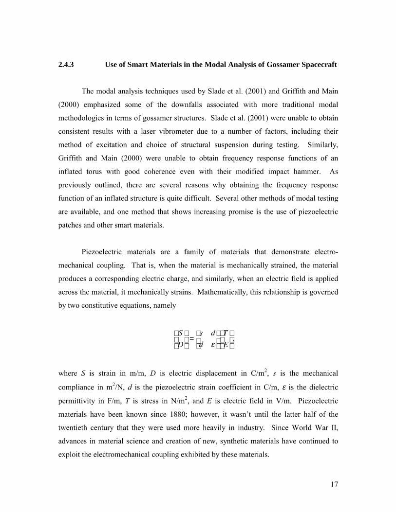
Piezoelectric materials are a family of materials that demonstrate electro-
mechanical coupling. That is, when the material is mechanically strained, the material
produces a corresponding electric charge, and similarly, when an electric field is applied
across the material, it mechanically strains. Mathematically, this relationship is governed
by two constitutive equations, namely
,
=
ET
dds
DS
ε
where S is strain in m/m, D is electric displacement in C/m2, s is the mechanical
compliance in m2/N, d is the piezoelectric strain coefficient in C/m, ε is the dielectric
permittivity in F/m, T is stress in N/m2, and E is electric field in V/m. Piezoelectric
materials have been known since 1880; however, it wasnt until the latter half of the
twentieth century that they were used more heavily in industry. Since World War II,
advances in material science and creation of new, synthetic materials have continued to
exploit the electromechanical coupling exhibited by these materials.
18
In 1998, Tzou provided the vibration community with an excellent review of
multiple smart materials and their corresponding applications. Tzous review includes
piezoelectric materials, shape memory alloys, magnetostrictive materials, and
magnetorhealogical fluids, to name but a few. Also in 1998, Wang wrote an article
outlining the use of piezoelectric patches as both actuators and sensors in the generation
of a system frequency response function. Wang used PZT (lead zirconate titanate)
patches as actuators and PVDF (polyvinylidene fluoride) patches as sensors to
mathematically derive the frequency response function generated through their use. He
provides excellent comparison charts between other methods of sensing and actuation.
The idea of using piezoelectric patches to obtain frequency response functions
and extracting modal parameters is a rather mature idea. In 1991, Rubenstein et al.
implemented multiple control laws via piezoceramic transducer sensors and actuators to
reject steady-state disturbances to a simply supported plate. In 1994, Sun et al. published
their work regarding structural modal analysis using collocated piezoelectric actuators
and sensors. Even in 1994 the authors realized that the attachment of conventional
transducers onto a testing structure may result in considerable errors in the extracted
system parameters, especially with lightweight and flexible structures (Sun et al., 1994).
The authors performed a modal analysis using collocated sensors and actuators on a
cantilevered beam. They supported the integration of PZT patches for modal analysis
because they found that the patches had negligible effect on the dynamics of a thin,
flexible beam undergoing vibration. Sun et al. (1995) published another work
investigating a new method that measures the coupled impedance of two PZT sensors to
extract the frequency response function of a thin, lightweight system in 1995.
In 2000, Sirohi and Chopra (2000a) investigated the behavior of piezoelectric
sheet actuators. In particular, the authors investigated the free strain response of the
actuators under DC excitation, as well as the magnitude and phase of the free strain
response under different excitation voltages and frequencies. Later that year, the authors
published another paper investigating the underlying advantages and disadvantages
associated with using piezoelectric strain sensors. Their research found that the
19
performance of piezoelectric sensors surpasses that of conventional type strain gages,
with much less signal conditioning required, especially in applications involving low
strain levels and high noise levels (2000b).
In 2000, Wang and Chen performed a modal analysis of a simply supported plate
using only PZT patches as actuators and PVDF patches as sensors. Wang and Chens
work included a theoretical development of the interaction between the smart actuators
and sensors with the steel plate, generation of a column in the frequency response
function matrix, generation of the plates mode shapes, and extraction of the plates
modal parameters. They acknowledged that smart materials have a major advantage
over the conventional structural testing [in that the] piezoceramic transducers can be
integrated into the structure, and that the idea of using smart materials for system
identification is also important to other applications such as structural vibration and
acoustic control (2000).
Agnes and Rogers (2000) tried to obtain a frequency response function of an
inflated structure. The inflated structure, a childrens swimming pool (5 foot major
diameter and 1 foot cross-sectional diameter) with the floor panel removed, was excited
using an electromagnetic shaker and, separately, with a PVDF patch. In both cases, the
vibratory response of the structure was measured using a laser vibrometer around the
perimeter of the face of the torus. The torus was hung vertically within a square frame
and attached to the frame by four equivalent springs. Both the shaker and the PVDF
patch excited the torus from 0-50 Hz. The authors used the multivariate mode indicator
function (MMIF) to identify the resonant frequencies of the torus. Further analysis was
deemed impossible, due to the presence of significant non-linear effects, noise
attributable to unmeasured disturbances, and the low level of signal in both tests (2000).
Concurrently with Agnes and Rogers, Briand et al. (2000) performed research on
an inflated tire inner tube using an electromagnetic shaker as the input and a PVDF
sensor as the output to generate a frequency response function. The authors were able to
excite the structure from 0-100 Hz, and obtained good coherence in their results. The
20
results of the modal analysis were then compared to a finite element model of the inner
tube, and the results were favorable. Throughout the article, the authors also discuss the
possibility of using SMA fabrics and films as actuators.
Park et al. (2001) performed a modal analysis of an inflated tire inner tube in
2001. The research team used an electromagnetic shaker as a point input to the torus, and
compared the frequency response functions generated using an accelerometer and PVDF
patches as sensors. The torus was suspended vertically using a long, elastic wire. The
authors used the unified matrix polynomial approach (UMPA) pseudo least squares
method to extract the modal parameters of the torus. The work also included an
investigation of bimorph actuators and macro fiber composite (MFC) actuators. The
MFC actuator is an experimental actuator from NASA Langley Research Center (Wilkie
et al., 2000). The advantages of using the bimorph or MFC for actuation in the modal
analysis included negligible mass loading effects and significantly less interference
with the suspension modes of the free-free torus than excitations from the shaker (2001).
Finally, the authors attempted to control the vibration of the 4th out-of-plane mode using a
positive position feedback controller. Both the bimorph actuator and MFC actuator were
able to reduce the vibration of the rubber torus by approximately 50%.
Although piezoelectric materials are only one of many possible solutions in
obtaining accurate modal analyses of inflatable structures, the piezoelectric family offers
other potential successes further down the line. New, highly flexible PZT patches, such
as the MFC actuator or PVDF sensor, can be fully integrated into the skin of an inflated
structure and have negligible effect on the dynamic parameters of the system. PZT
patches can act as sensors and actuators, a condition known as self-sensing (Dosch et
al., 1992). And in terms of vibration control, piezoelectric materials offer the potential
for controlled vibration suppression.

21
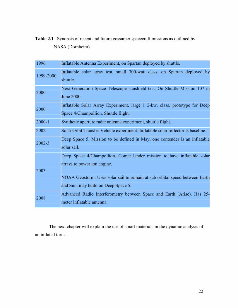
2.5 The Future of Gossamer Spacecraft Technology
Vibration control of gossamer spacecraft and membranes on the order of microns
is critical to future mission success. The achievement of such tight vibration tolerances is
the motivation behind the dynamic parameter identification and the active vibration
control experiments of the Kapton torus in this thesis. Piezoelectric materials are one
possible answer to the proposed problem.
Another potential benefit of pursuing the marriage of piezoelectric technology and
gossamer spacecraft is the possibility of on-orbit shape control. In 1994, Salama et al.
proposed the use of piezo-induced deformations to achieve a higher degree of on-orbit
surface accuracy with inflatable antennas. Given recent advances in the fabrication of
PVDF and MFC materials, shape control of gossamer spacecraft is now not only feasible
but also cost effective.
NASA is considering gossamer technology in its future Space Shuttle missions.
Table 2.1 outlines NASAs Space Shuttle missions integrated with gossamer technology,
starting with the launching of the Inflatable Antenna Experiment in 1996.
22
Table 2.1. Synopsis of recent and future gossamer spacecraft missions as outlined by
NASA (Dornheim).
1996 Inflatable Antenna Experiment, on Spartan deployed by shuttle.
1999-2000 Inflatable solar array test, small 300-watt class, on Spartan deployed by
shuttle.
2000 Next-Generation Space Telescope sunshield test. On Shuttle Mission 107 in
June 2000.
2000 Inflatable Solar Array Experiment, large 1 2-kw. class, prototype for Deep
Space 4/Champollion. Shuttle flight.
2000-1 Synthetic aperture radar antenna experiment, shuttle flight.
2002 Solar Orbit Transfer Vehicle experiment. Inflatable solar reflector is baseline.
2002-3 Deep Space 5. Mission to be defined in May, one contender is an inflatable
solar sail.
2003
Deep Space 4/Champollion. Comet lander mission to have inflatable solar
arrays to power ion engine.
NOAA Geostorm. Uses solar sail to remain at sub orbital speed between Earth
and Sun, may build on Deep Space 5.
2008 Advanced Radio Interferometry between Space and Earth (Arise). Has 25-
meter inflatable antenna.
The next chapter will explain the use of smart materials in the dynamic analysis of
an inflated torus.
23
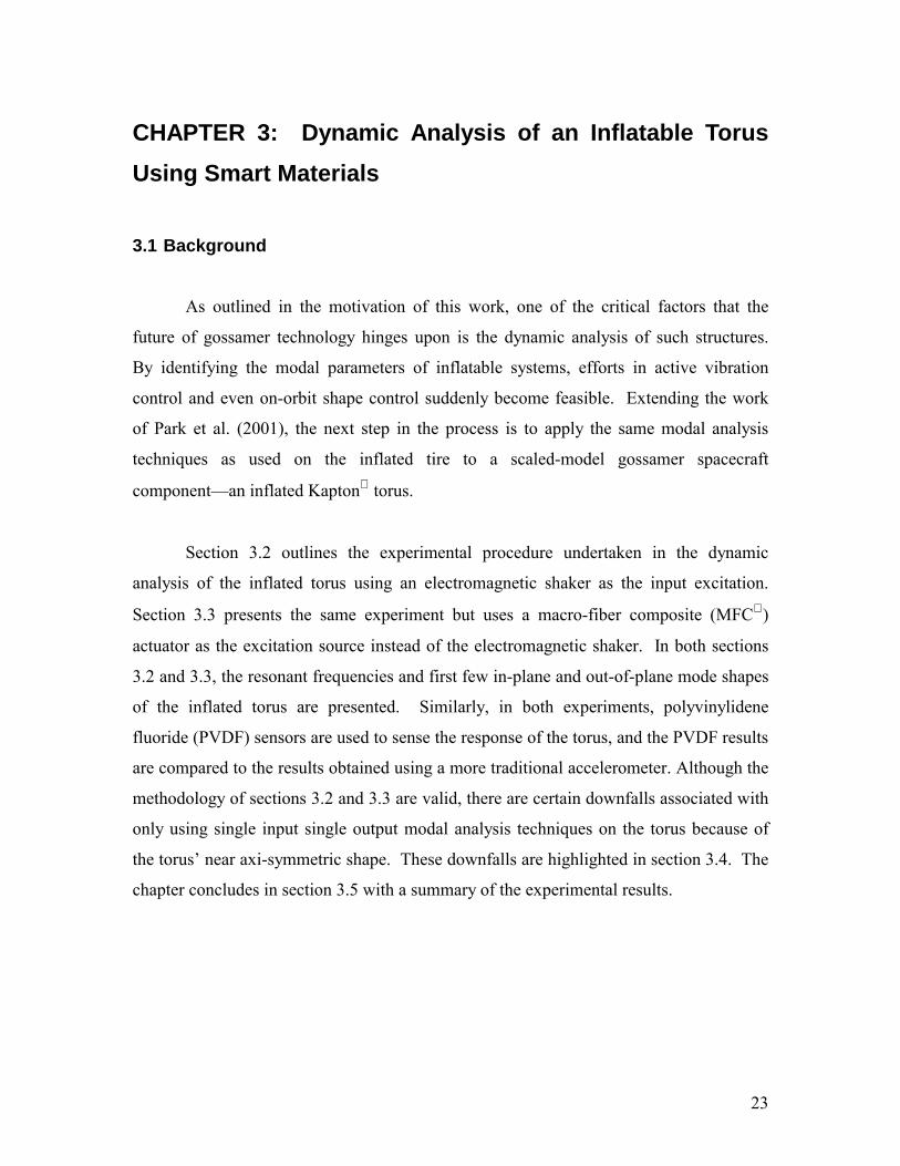
CHAPTER 3: Dynamic Analysis of an Inflatable Torus Using Smart Materials
3.1 Background
As outlined in the motivation of this work, one of the critical factors that the
future of gossamer technology hinges upon is the dynamic analysis of such structures.
By identifying the modal parameters of inflatable systems, efforts in active vibration
control and even on-orbit shape control suddenly become feasible. Extending the work
of Park et al. (2001), the next step in the process is to apply the same modal analysis
techniques as used on the inflated tire to a scaled-model gossamer spacecraft
componentan inflated Kapton torus.
Section 3.2 outlines the experimental procedure undertaken in the dynamic
analysis of the inflated torus using an electromagnetic shaker as the input excitation.
Section 3.3 presents the same experiment but uses a macro-fiber composite (MFC )
actuator as the excitation source instead of the electromagnetic shaker. In both sections
3.2 and 3.3, the resonant frequencies and first few in-plane and out-of-plane mode shapes
of the inflated torus are presented. Similarly, in both experiments, polyvinylidene
fluoride (PVDF) sensors are used to sense the response of the torus, and the PVDF results
are compared to the results obtained using a more traditional accelerometer. Although the
methodology of sections 3.2 and 3.3 are valid, there are certain downfalls associated with
only using single input single output modal analysis techniques on the torus because of
the torus near axi-symmetric shape. These downfalls are highlighted in section 3.4. The
chapter concludes in section 3.5 with a summary of the experimental results.
24
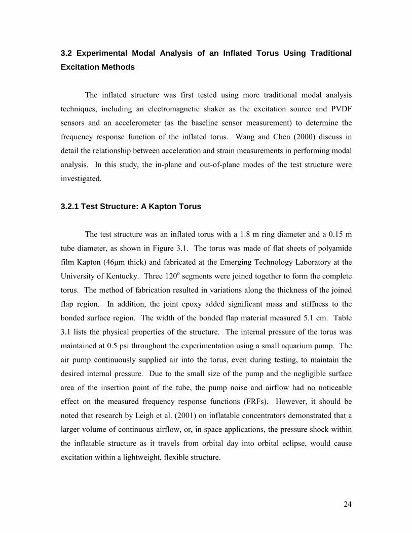
3.2 Experimental Modal Analysis of an Inflated Torus Using Traditional Excitation Methods
The inflated structure was first tested using more traditional modal analysis
techniques, including an electromagnetic shaker as the excitation source and PVDF
sensors and an accelerometer (as the baseline sensor measurement) to determine the
frequency response function of the inflated torus. Wang and Chen (2000) discuss in
detail the relationship between acceleration and strain measurements in performing modal
analysis. In this study, the in-plane and out-of-plane modes of the test structure were
investigated.
3.2.1 Test Structure: A Kapton Torus
The test structure was an inflated torus with a 1.8 m ring diameter and a 0.15 m
tube diameter, as shown in Figure 3.1. The torus was made of flat sheets of polyamide
film Kapton (46µm thick) and fabricated at the Emerging Technology Laboratory at the
University of Kentucky. Three 120o segments were joined together to form the complete
torus. The method of fabrication resulted in variations along the thickness of the joined
flap region. In addition, the joint epoxy added significant mass and stiffness to the
bonded surface region. The width of the bonded flap material measured 5.1 cm. Table
3.1 lists the physical properties of the structure. The internal pressure of the torus was
maintained at 0.5 psi throughout the experimentation using a small aquarium pump. The
air pump continuously supplied air into the torus, even during testing, to maintain the
desired internal pressure. Due to the small size of the pump and the negligible surface
area of the insertion point of the tube, the pump noise and airflow had no noticeable
effect on the measured frequency response functions (FRFs). However, it should be
noted that research by Leigh et al. (2001) on inflatable concentrators demonstrated that a
larger volume of continuous airflow, or, in space applications, the pressure shock within
the inflatable structure as it travels from orbital day into orbital eclipse, would cause
excitation within a lightweight, flexible structure.
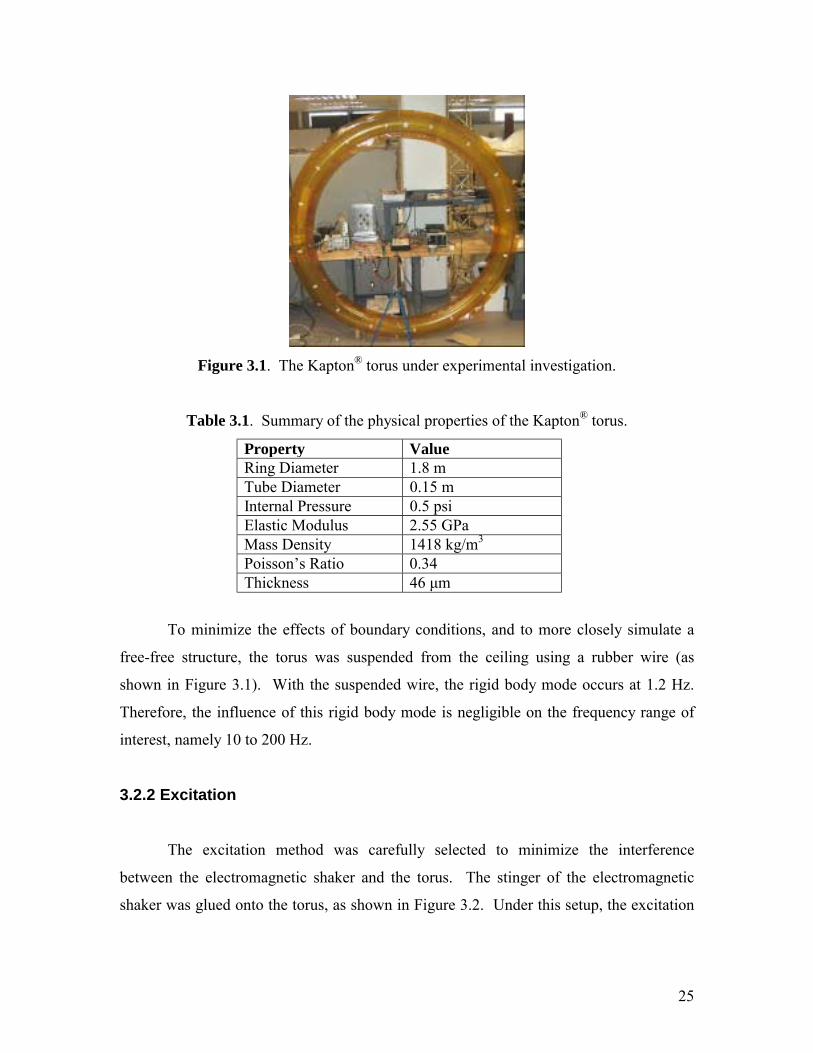
25
Figure 3.1. The Kapton® torus under experimental investigation.
Table 3.1. Summary of the physical properties of the Kapton® torus.
Property Value Ring Diameter 1.8 m Tube Diameter 0.15 m Internal Pressure 0.5 psi Elastic Modulus 2.55 GPa Mass Density 1418 kg/m3 Poissons Ratio 0.34 Thickness 46 µm
To minimize the effects of boundary conditions, and to more closely simulate a
free-free structure, the torus was suspended from the ceiling using a rubber wire (as
shown in Figure 3.1). With the suspended wire, the rigid body mode occurs at 1.2 Hz.
Therefore, the influence of this rigid body mode is negligible on the frequency range of
interest, namely 10 to 200 Hz.
3.2.2 Excitation
The excitation method was carefully selected to minimize the interference
between the electromagnetic shaker and the torus. The stinger of the electromagnetic
shaker was glued onto the torus, as shown in Figure 3.2. Under this setup, the excitation
26
was considered to be a unidirectional point input, and could be configured for either in-
plane or out-of-plane excitation.
Figure 3.2. Electromagnetic shaker attachment to the skin of the torus.
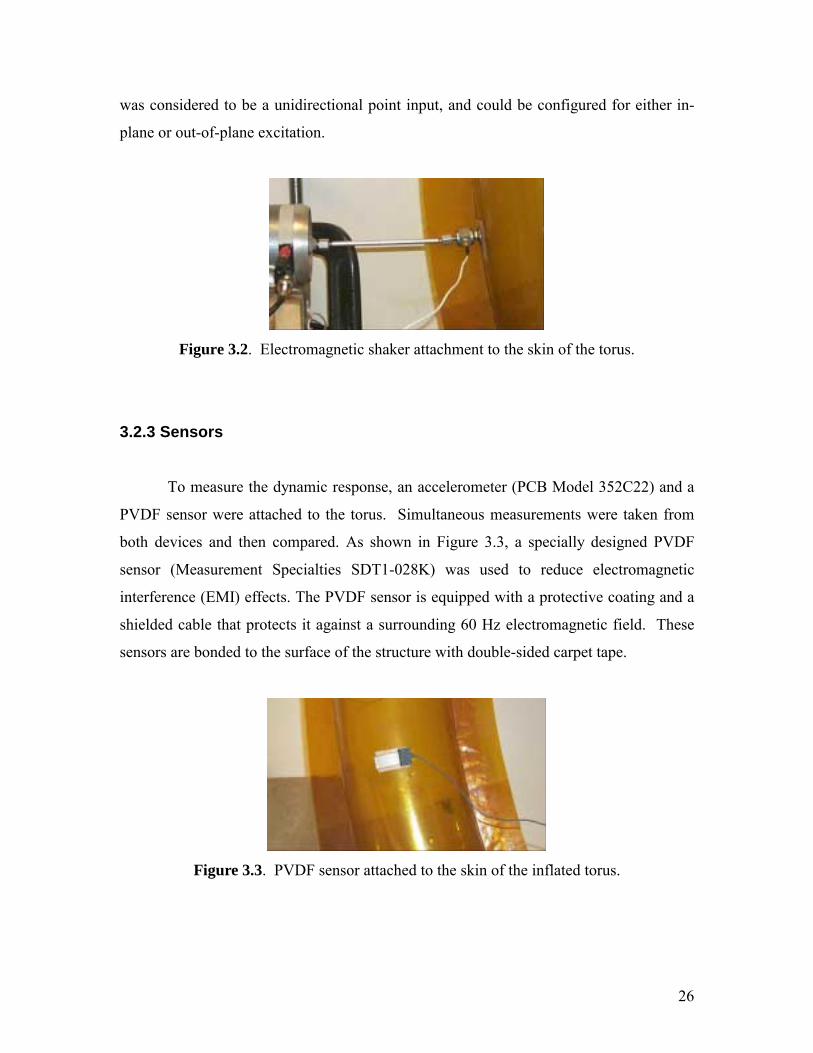
3.2.3 Sensors
To measure the dynamic response, an accelerometer (PCB Model 352C22) and a
PVDF sensor were attached to the torus. Simultaneous measurements were taken from
both devices and then compared. As shown in Figure 3.3, a specially designed PVDF
sensor (Measurement Specialties SDT1-028K) was used to reduce electromagnetic
interference (EMI) effects. The PVDF sensor is equipped with a protective coating and a
shielded cable that protects it against a surrounding 60 Hz electromagnetic field. These
sensors are bonded to the surface of the structure with double-sided carpet tape.
Figure 3.3. PVDF sensor attached to the skin of the inflated torus.
27
3.2.4 Experimental Procedure
The torus was excited in the out-of-plane direction and in the radial (in-plane)
direction to measure the out-of-plane and in-plane modes. For acquisition of the toruss
modal parameters in either direction, the sensors were arranged at sixteen evenly spaced
locations (as shown by the white tape marks in Figure 3.1).
Force, acceleration, and strain (from PVDF sensors) data were collected through a
DSPT SigLab multi-channel dynamic signal analyzer. A chirp signal excited the
structure from 5 to 100 Hz. To ensure enough input energy at each frequency from
excitation, the chirp input frequency for each test was divided into three sub-ranges (5-
35, 35-65, and 65-100 Hz). Furthermore, the time period of excitation was held for as
long as possible (130,000 samples at each sub-range) so that the excitation ceased and
that the corresponding response signal in a data frame was damped out (Guan et al.,
2000). Control of the excitation signal length was realized using a sampling number
function in the SigLab signal analyzer. The careful selection of excitation signal (specific
length and bandwidth) was found to be critical for a flexible inflatable torus when trying
to obtain reliable vibratory responses with reasonable accuracy. Ten runs were averaged
to estimate the frequency response functions.
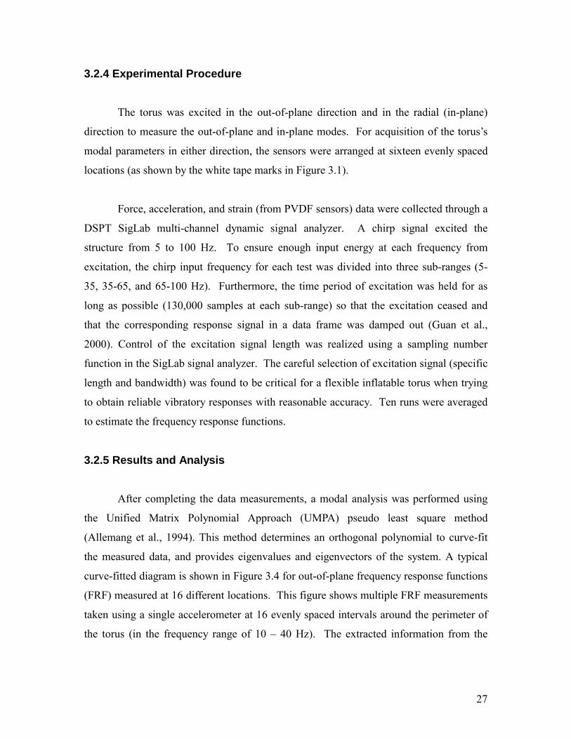
3.2.5 Results and Analysis
After completing the data measurements, a modal analysis was performed using
the Unified Matrix Polynomial Approach (UMPA) pseudo least square method
(Allemang et al., 1994). This method determines an orthogonal polynomial to curve-fit
the measured data, and provides eigenvalues and eigenvectors of the system. A typical
curve-fitted diagram is shown in Figure 3.4 for out-of-plane frequency response functions
(FRF) measured at 16 different locations. This figure shows multiple FRF measurements
taken using a single accelerometer at 16 evenly spaced intervals around the perimeter of
the torus (in the frequency range of 10 40 Hz). The extracted information from the
28
UMPA pseudo least square method was input to a MATLab program to plot the resulting
mode shapes at resonant frequencies.
Figure 3.4. A sample curve-fitted FRF from the collected modal data using the
UMPA pseudo least squares method.
From the modal analysis, three main types of mode shapes were identified. The
structure not only demonstrated ring (in-plane and out-of-plane) mode shapes, but also
demonstrated shell mode shapes at some resonant frequencies. Lewiss finite element
study (Lewis, 2000) demonstrates the significant impact various aspect ratios play on the
mode shapes of a toroidal structure. In his study, the vibratory response of a torus is
dominated by shell modes if the aspect ratio is greater than 0.3, but, for a torus of small
aspect ratio (less than 0.1), the shell mode activities are less significant. Similarly, the
detailed FEA model developed by Leigh et al. (2001) also predicted similar shell
behavior from a torus.
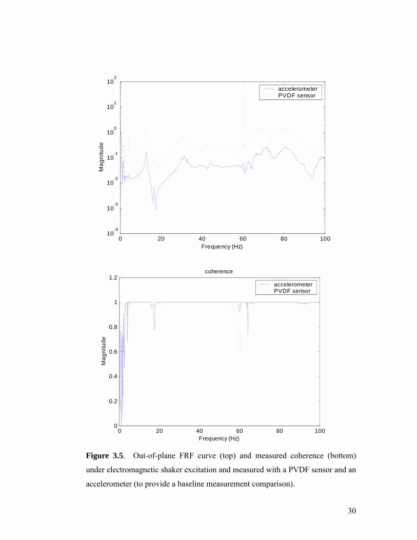
Figure 3.5 shows transfer functions of the out-of-plane motion measured with the
accelerometer and the PVDF sensors. The coherence plot, which indicates the correlation
between a single input and a single output measurement, is also shown to indicate that the
29
test results are reasonable. Both FRF curves contain distinct resonant frequencies near 13
and 32 Hz at the first two out-of plane resonant frequencies. Another resonant peak is
identifiable near 65 Hz, but hard to distinguish from a shell mode near the same
frequency. The offset seen between the PVDF sensor FRF curve and the accelerometer
FRF curve in Figure 3.5 is caused by the amplification of the PVDF signal by the SigLab
data acquisition system. Since the FRF curve is a ratio of the output signal to input
signal, the amplification of the PVDF signal shifts the FRF curve vertically. Further, at
another sensor location, the two signals may be very different in nature, but they will
share the same resonant frequency peaks.
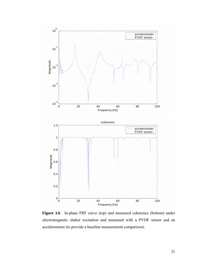
Figure 3.6 shows a sample transfer function measured in the in-plane direction.
The first two resonant peaks are identified near 16 and 42 Hz as the in-plane modes.
However, as the frequency increases, it is harder to identify resonant frequencies because
of the presence of numerous shell modes. The apparent spike in the PVDF FRF curves in
both Figures 3.5 and 3.6 is the result of an electromagnetic interference effect from
surrounding electronic equipment at 60 Hz. The relatively small size of the sensor made
it susceptible to the EMI effect, even with its shielded coating.
30
0 20 40 60 80 10010
-4
10-3
10-2
10-1
100
101
102
Frequency (Hz)
Mag
nitu
de
accelerometerPVDF sensor
0 20 40 60 80 1000
0.2
0.4
0.6
0.8
1
1.2
Frequency (Hz)
Mag
nitu
de
coherence
accelerometerPVDF sensor
Figure 3.5. Out-of-plane FRF curve (top) and measured coherence (bottom)
under electromagnetic shaker excitation and measured with a PVDF sensor and an
accelerometer (to provide a baseline measurement comparison).
31
0 20 40 60 80 100
10-4
10-3
10-2
10-1
100
Frequency (Hz)
Mag
nitu
de
accelerometerPVDF sensor
0 20 40 60 80 1000
0.2
0.4
0.6
0.8
1
1.2
Frequency (Hz)
Mag
nitu
de
coherence
accelerometerPVDF sensor
Figure 3.6. In-plane FRF curve (top) and measured coherence (bottom) under
electromagnetic shaker excitation and measured with a PVDF sensor and an
accelerometer (to provide a baseline measurement comparison).
32
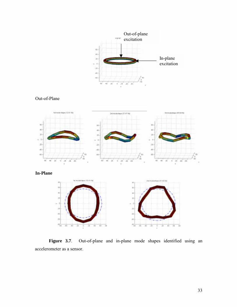
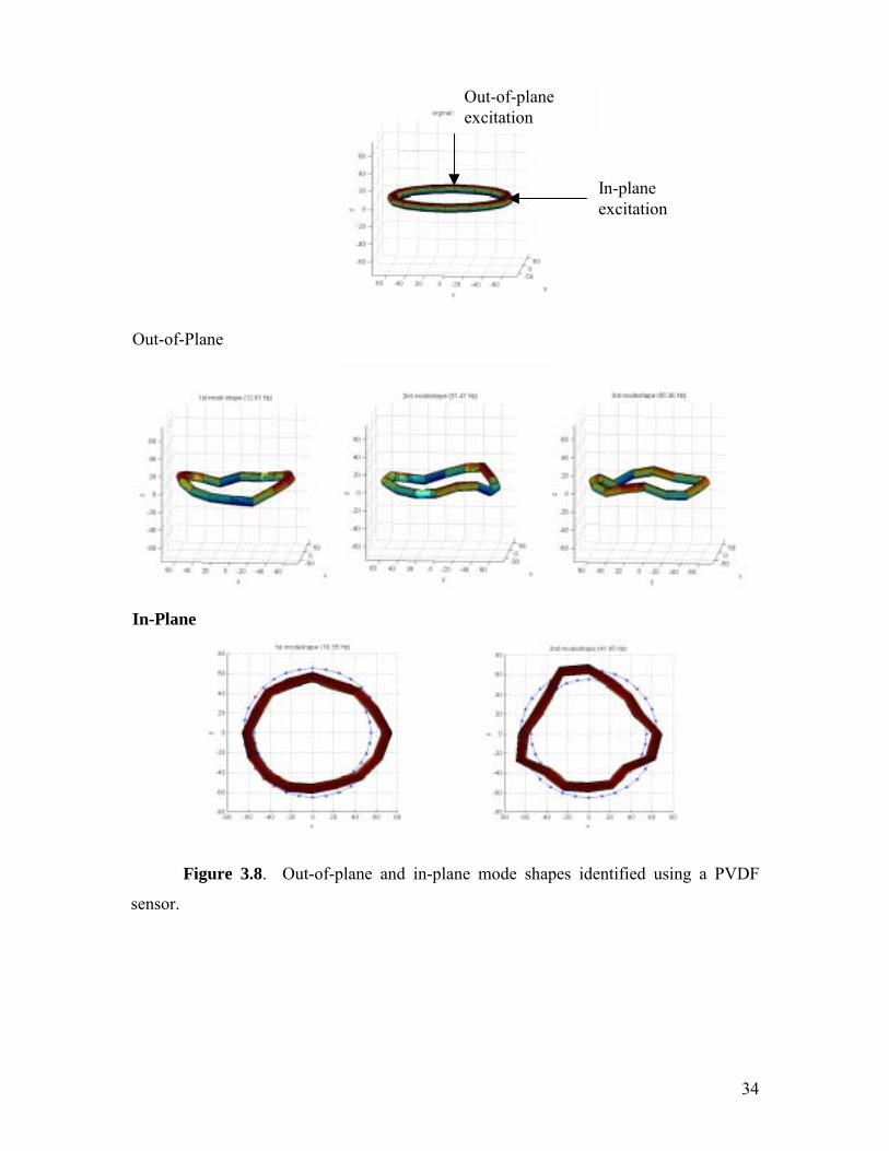
Mode shapes contain important information for identifying the nature of resonant
frequencies (i.e. in-plane, out-of-plane, or shell modes). FRFs alone are inadequate for
determining the nature of a resonant frequency, especially near shell mode activity.
Therefore, from the collected curve-fitted data, the mode shapes associated with each
resonant frequency were plotted in MATLab. As found with finite element techniques, a
structures mode shapes are expected to have a sequential number of nodal lines
(Allemang et al., 1994). Therefore, from the collected in-plane and out-of-plane data and
under this assumption, we were able to identify the ring mode shapes and differentiate
them from the shell modes. Figures 3.7 and 3.8 show the first three out-of-plane resonant
frequency mode shapes, and the first two in-plane resonant frequency mode shapes, using
an accelerometer and a PVDF sensor, respectively. These mode shapes are generated
using the FRF analysis results extracted from the UMPA pseudo least square method.
The discrepancy between the apparent smoothness of mode shapes in Figures 3.7 and 3.8
is attributed to imperfect bonding between the PVDF sensor and the double-sided tape
used to attach the sensor to the skin of the torus. PVDF sensor results are expected to be
more accurate if the sensors are permanently fixed to the skin of a torus with a better
adhesive, such as super glue. Table 3.2 summarizes the modal results.
33
Out-of-Plane
In-Plane
Figure 3.7. Out-of-plane and in-plane mode shapes identified using an
accelerometer as a sensor.
In-plane excitation
Out-of-plane excitation
34
Out-of-Plane
In-Plane
Figure 3.8. Out-of-plane and in-plane mode shapes identified using a PVDF
sensor.
In-plane excitation
Out-of-plane excitation
35
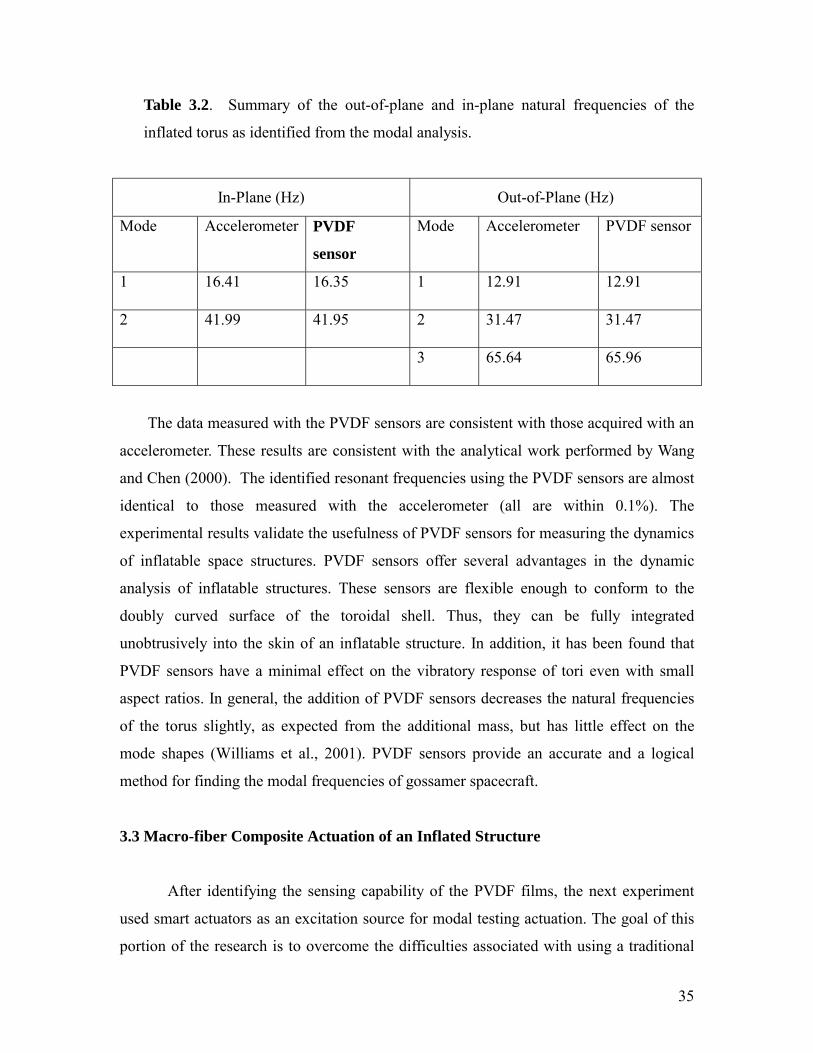
Table 3.2. Summary of the out-of-plane and in-plane natural frequencies of the
inflated torus as identified from the modal analysis.
In-Plane (Hz) Out-of-Plane (Hz)
Mode Accelerometer PVDF
sensor
Mode Accelerometer PVDF sensor
1 16.41 16.35 1 12.91 12.91
2 41.99 41.95 2 31.47 31.47
3 65.64 65.96
The data measured with the PVDF sensors are consistent with those acquired with an
accelerometer. These results are consistent with the analytical work performed by Wang
and Chen (2000). The identified resonant frequencies using the PVDF sensors are almost
identical to those measured with the accelerometer (all are within 0.1%). The
experimental results validate the usefulness of PVDF sensors for measuring the dynamics
of inflatable space structures. PVDF sensors offer several advantages in the dynamic
analysis of inflatable structures. These sensors are flexible enough to conform to the
doubly curved surface of the toroidal shell. Thus, they can be fully integrated
unobtrusively into the skin of an inflatable structure. In addition, it has been found that
PVDF sensors have a minimal effect on the vibratory response of tori even with small
aspect ratios. In general, the addition of PVDF sensors decreases the natural frequencies
of the torus slightly, as expected from the additional mass, but has little effect on the
mode shapes (Williams et al., 2001). PVDF sensors provide an accurate and a logical
method for finding the modal frequencies of gossamer spacecraft.
3.3 Macro-fiber Composite Actuation of an Inflated Structure
After identifying the sensing capability of the PVDF films, the next experiment
used smart actuators as an excitation source for modal testing actuation. The goal of this
portion of the research is to overcome the difficulties associated with using a traditional
36
shaker input-accelerometer output test. Furthermore, the actuator, if incorporated in an
active control scheme, has the potential to actively suppress the vibration of an inflatable
structure.
The following experimental procedure is an extension of Park et al.s (2001)
previous work on applying smart actuators, such as an MFC , to an inflatable structure,
but is closer in scale, aspect ratio, and in material of an actual space structure. The MFC
offers high performance and flexibility suitable for applications with inflatable structures.
A summary of representative properties and applications of the MFC device can be
found in the Appendix.
3.3.1 Experimental Configuration of the MFC Actuator
Experiments were performed using the MFC actuator as the excitation device of
an inflated torus. The same configuration was used as described in the shaker-input
experiment in section 3.2.4. The actuator was bonded to the surface of the torus with
double-sided tape, as shown in Figure 3.9. The SigLab analyzer produced an 8 V chirp
signal varying from 10-200 Hz. The input signal was then amplified by a factor of 100
through a TREK High Voltage Power Supply (model 50/750), and thus applied 800 volts
to the actuator. Both an accelerometer and a PVDF sensor were used to measure the
dynamic response.
Figure 3.9. MFC actuator attached to the skin of the torus with double-sided
carpet tape.

37
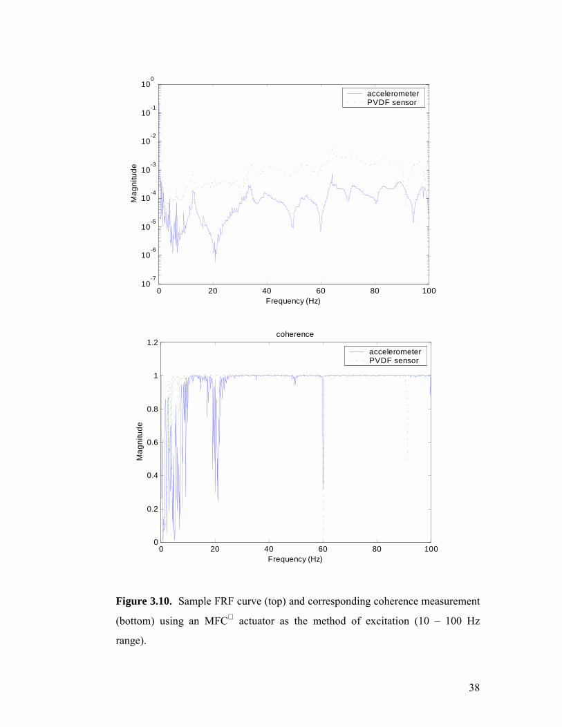
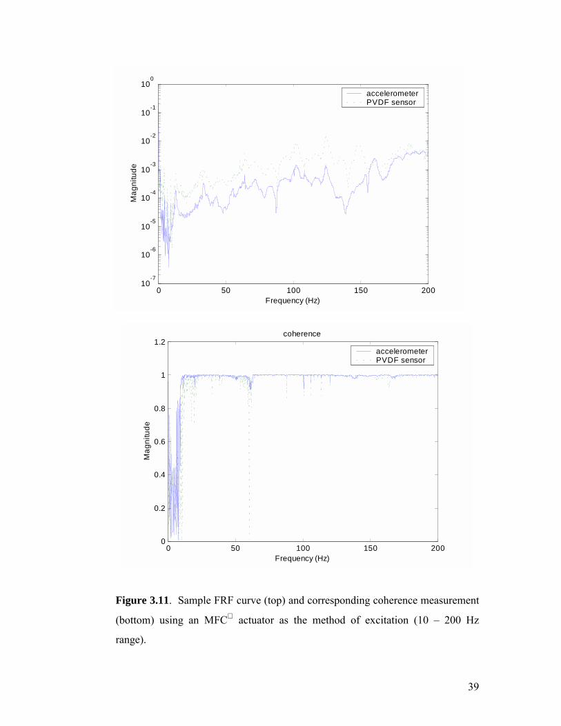
3.3.2 Results and Analysis
A group of typical frequency response and coherence curves resulting from
MFC actuation are illustrated in Figures 3.10 and 3.11. As shown, the MFC actuation
is effective up to 200 Hz, where the shaker was only able to excite up to 100 Hz. In
addition, the sensors clearly pick up the signal 180 degrees apart from the actuator (on
both sides), which indicates that the actuator is able to excite the entire torus. However,
there are some limitations associated with the SISO methodology presented, and such
limitations will be discussed in section 3.4.
38
0 20 40 60 80 100
10-7
10-6
10-5
10-4
10-3
10-2
10-1
100
Frequency (Hz)
Mag
nitu
de
accelerometerPVDF sensor
0 20 40 60 80 1000
0.2
0.4
0.6
0.8
1
1.2
Frequency (Hz)
Mag
nitu
de
coherence
accelerometerPVDF sensor
Figure 3.10. Sample FRF curve (top) and corresponding coherence measurement
(bottom) using an MFC actuator as the method of excitation (10 100 Hz
range).
39
0 50 100 150 200
10-7
10-6
10-5
10-4
10-3
10-2
10-1
100
Frequency (Hz)
Mag
nitu
de
accelerometerPVDF sensor
0 50 100 150 2000
0.2
0.4
0.6
0.8
1
1.2
Frequency (Hz)
Mag
nitu
de
coherence
accelerometerPVDF sensor
Figure 3.11. Sample FRF curve (top) and corresponding coherence measurement
(bottom) using an MFC actuator as the method of excitation (10 200 Hz
range).
40
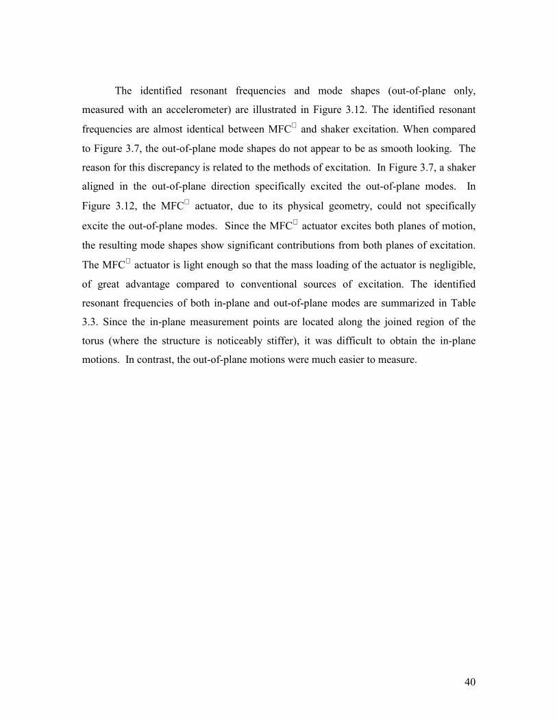
The identified resonant frequencies and mode shapes (out-of-plane only,
measured with an accelerometer) are illustrated in Figure 3.12. The identified resonant
frequencies are almost identical between MFC and shaker excitation. When compared
to Figure 3.7, the out-of-plane mode shapes do not appear to be as smooth looking. The
reason for this discrepancy is related to the methods of excitation. In Figure 3.7, a shaker
aligned in the out-of-plane direction specifically excited the out-of-plane modes. In
Figure 3.12, the MFC actuator, due to its physical geometry, could not specifically
excite the out-of-plane modes. Since the MFC actuator excites both planes of motion,
the resulting mode shapes show significant contributions from both planes of excitation.
The MFC actuator is light enough so that the mass loading of the actuator is negligible,
of great advantage compared to conventional sources of excitation. The identified
resonant frequencies of both in-plane and out-of-plane modes are summarized in Table
3.3. Since the in-plane measurement points are located along the joined region of the
torus (where the structure is noticeably stiffer), it was difficult to obtain the in-plane
motions. In contrast, the out-of-plane motions were much easier to measure.
41
Figure 3.12. Identified out-of-plane mode shapes using an accelerometer as a
sensor and an MFC actuator as the input energy device. The mode shapes are
numbered to show increasing nodal lines at higher frequencies.
1 2
3 4
42
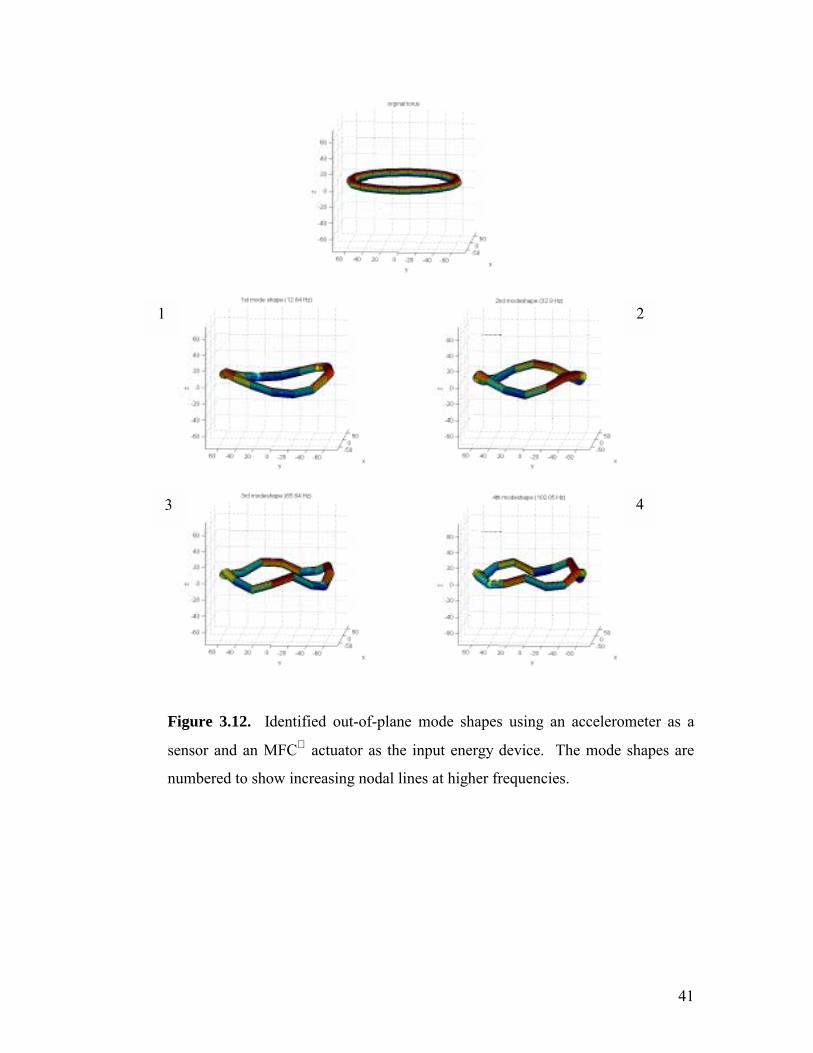
Table 3.3. Identified in-plane and out-of-plane resonant frequencies of the inflated torus
using an MFC actuator as the input energy device.
In-Plane (Hz) Out-of-Plane (Hz)
Mode Accelerometer PVDF sensor Mode Accelerometer PVDF sensor
1 16.37 16.31 1 12.84 12.81
2 40.24 40.74 2 32.9 31.7
3 68.1 67.78 3 65.64 65.4
4 102.05 100.92
It was obvious during the tests that the MFC excitation produced less
interference with suspension modes of the free-free torus than excitations from the
shaker. Without connections to the ground (except for an electrical cable), these actuators
and the PVDF sensor can be considered an integral part of an inflated structure. The
MFC -PVDF combination could also be used as control devices of an inflatable structure
for both vibration suppression and static shape control.
3.4 The Limitations of SISO Experimentation
Single input single output (SISO) experimental modal analysis techniques are cost
effective and relatively straightforward methods of structural dynamic analysis.
However, SISO dynamic analysis techniques are limited in terms of their ability to
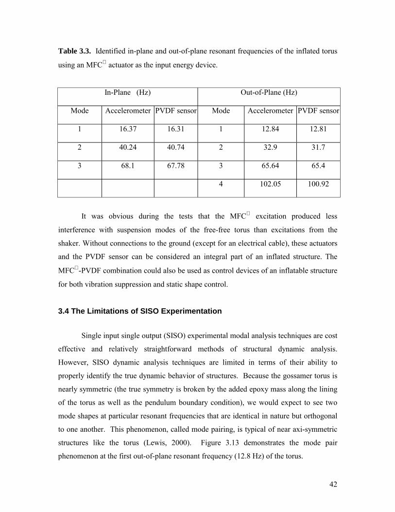
properly identify the true dynamic behavior of structures. Because the gossamer torus is
nearly symmetric (the true symmetry is broken by the added epoxy mass along the lining
of the torus as well as the pendulum boundary condition), we would expect to see two
mode shapes at particular resonant frequencies that are identical in nature but orthogonal
to one another. This phenomenon, called mode pairing, is typical of near axi-symmetric
structures like the torus (Lewis, 2000). Figure 3.13 demonstrates the mode pair
phenomenon at the first out-of-plane resonant frequency (12.8 Hz) of the torus.
43
Figure 3.13. Orthogonal mode pair of an axi-symmetric torus found at the first
out-of-plane resonant frequency. The cross-section of each mode pair is also
shown.
Unfortunately, the separation between the mode pairs may be at such a small scale
that the signal noise of the sensor or the resolution of the data acquisition system may not
be able to distinguish the two resonant responses. Or, in a more likely fashion, the dual
peaks may be smeared together as one, and consequently be misinterpreted as a single
mode. One method of trying to correct this problem is to increase the number of inputs
and outputs of our experimental modal analysis. The benefits of a multiple input multiple
output modal methodology will be discussed in the next chapter.
3.5 Chapter Summary
In this experiment, the extremely flexible nature of the inflatable torus made
collecting modal parameter information quite difficult. In particular, local excitation with
a shaker and a MFC as a point input only exaggerated the local properties of the
structure. To eliminate the localized effect, the structure was excited over a small
bandwidth (30 Hz) and the sampling rate of the SigLab Analyzer was consequently
increased. By focusing on the small bandwidth, the entire structure was provided with
sufficient input energy, and the global modes were thereby excited. Also, by increasing
the sampling rate, the signal analyzer was able to extract most of the modal

44
characteristics of the torus. SISO experiments are easy to perform, do not require
expensive hardware, and can be used to get a strong understanding of the dynamic
behavior of a structure.
Although the previous two experiments demonstrated the feasibility of using
smart materials to obtain reliable FRF measurements, the ability of the SISO technique to
accurately extract the modal pairs of the torus is highly doubted. Further, the question
remains as to whether the MFC actuators have enough actuation authority to excite the
global modes of a true gossamer space structure, which could be up to 25 m in diameter.
Chapter 4 explores the use of multiple actuators and sensors in the dynamic
characterization of a gossamer structure.
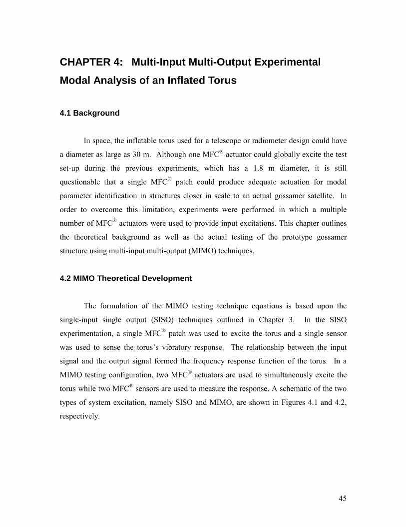
45
CHAPTER 4: Multi-Input Multi-Output Experimental Modal Analysis of an Inflated Torus
4.1 Background
In space, the inflatable torus used for a telescope or radiometer design could have
a diameter as large as 30 m. Although one MFC® actuator could globally excite the test
set-up during the previous experiments, which has a 1.8 m diameter, it is still
questionable that a single MFC® patch could produce adequate actuation for modal
parameter identification in structures closer in scale to an actual gossamer satellite. In
order to overcome this limitation, experiments were performed in which a multiple
number of MFC® actuators were used to provide input excitations. This chapter outlines
the theoretical background as well as the actual testing of the prototype gossamer
structure using multi-input multi-output (MIMO) techniques.
4.2 MIMO Theoretical Development
The formulation of the MIMO testing technique equations is based upon the
single-input single output (SISO) techniques outlined in Chapter 3. In the SISO
experimentation, a single MFC® patch was used to excite the torus and a single sensor
was used to sense the toruss vibratory response. The relationship between the input
signal and the output signal formed the frequency response function of the torus. In a
MIMO testing configuration, two MFC® actuators are used to simultaneously excite the
torus while two MFC® sensors are used to measure the response. A schematic of the two
types of system excitation, namely SISO and MIMO, are shown in Figures 4.1 and 4.2,
respectively.
46
With two actuators and two sensors in place, we can estimate frequency response
functions with a few experiments. Two experiments (as shown in Figure 4.2) will give
the following FRF matrix:
=2221
12111 HH
HHH , (4.1)
where a
a
XYH 1
11 = ,a
a
XYH 2
21 = ,b
a
XYH 1
12 = , b
a
XYH 2
22 = . In the formulation, Y refers to the
sensor output at a given MFC® sensor, and X refers to the input signal to a given MFC®
actuator.
Each column of the FRF matrix can be constructed during the experiment in a
SISO experiment. This is common practice in modal testing for almost all structures.
However, for flexible, large-scale inflatable structures, only exciting a single point may
cause poor distribution of input energy throughout the structure and result in somewhat
distorted frequency responses.
1
2
1
2
Xa Y1a
Y1b
1
2
1
2 Xb
Y1a
Y1b
Test 1
Test 2
Figure 4.1. SISO tests to estimate FRFs.
actuator sensors
Test 1 1
2
1
2
Xc Y1c
Y2c
1
2
1
2
Xd Y1d
Y2d
Test 2
+
+
+
-
Figure 4.2. MIMO tests to estimate FRFs.
actuator sensors

47
For the multi-input testing, a single in-phase signal is applied to both actuators for
the first experiment (test 1 in Figure 4.2) and, for the second experiment (test 2 in Figure
4.2), a single out-of-phase signal is supplied to both actuators, as illustrated by the +
and signs.
By using a multi-input test, we can estimate the same FRF matrix after a post-
processing procedure. This method provides better energy distribution and even better
actuation forces. The method is based on the multi-phase stepped sine test, but may
also be used with a chirp signal. In either case, it is imperative that the transient response
at the tail end of the frequency sweep is allowed to completely die out (Guan et al.,
2000); otherwise, uncorrelated data will be introduced into the averaged FRF. In order to
estimate the FRF matrix, the following procedure is required.
For test 1,
cc
c
c
c XHXX
HYY
=
=
11
2
1
and for test 2,
dd
d
d
d XHX
XH
YY
−
=
−
=
11
2
1
By dividing Equations (4.2) and (4.3) by Xc and Xd, respectively, we get
=
=
11
2
1
2
1
HXH
XY
XY
c
c
c
c
c
c
,

48
−
=
=
11
2
1
2
1
HXH
XY
XY
d
d
d
d
d
d
.
And by adding the two columns leads to
−
=
11
11
22
11 HHHHH
dc
dc .
Now, the FRF matrix, H, can be constructed by post-multiplying by the inverse of the
matrix in Equation (4.6). Theoretically, the FRF matrix H1 (in Equation (4.1)) and H (in
Equation (4.6)) must be the same, unless the structure shows significant non-linearity.
Only two pairs of sensors/actuators are described in this section, but one may use any
number of actuators if necessary.
4.3 The MIMO Experiment Experiments were performed following the procedure outlined in section 4.2. Four
MFC® patches were attached to the torus at 90 degree intervals as shown in Figure 4.3.
First, the torus was checked for non-linearity in the first few modes of interest. Then the
FRFs, both SISO and MIMO, were measured and compared. The torus was maintained at
0.75 psi during this phase of the experimentation.
Figure 4.3. Experimental setup with multiple sensors and actuators.
Actuator 1 Actuator 2
Sensor 1 Sensor 2
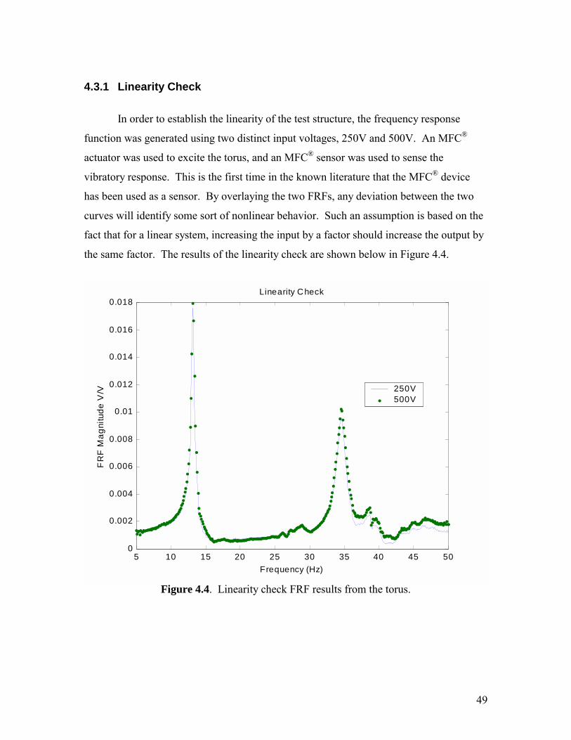
49
4.3.1 Linearity Check
In order to establish the linearity of the test structure, the frequency response
function was generated using two distinct input voltages, 250V and 500V. An MFC®
actuator was used to excite the torus, and an MFC® sensor was used to sense the
vibratory response. This is the first time in the known literature that the MFC® device
has been used as a sensor. By overlaying the two FRFs, any deviation between the two
curves will identify some sort of nonlinear behavior. Such an assumption is based on the
fact that for a linear system, increasing the input by a factor should increase the output by
the same factor. The results of the linearity check are shown below in Figure 4.4.
5 10 15 20 25 30 35 40 45 500
0.002
0.004
0.006
0.008
0.01
0.012
0.014
0.016
0.018Linearity Check
Frequency (Hz)
FR
F M
agni
tude
V/V 250V
500V
Figure 4.4. Linearity check FRF results from the torus.
50
As shown in Figure 4.4, the torus primarily demonstrates linear system behavior
from 5 - 50 Hz. Therefore, the theoretical development for a MIMO testing technique as
presented in section 4.2 should be applicable to the torus.
4.3.2 MIMO Experimental Results
The experiment was performed using similar data acquisition techniques outlined
in Chapter 3. A chirp signal was applied to the torus sweeping from 5 to 50 Hz. The
signal was applied for 4 seconds, and then turned off for 4 seconds. The burst chirp
signal effectively allowed the transient response of the torus to die out before the next
FRF curve was estimated (Guan et al., 2000). A series of ten averages were used in the
FRF estimation. As shown in Figure 4.5, the MIMO testing identifies better FRFs with
higher coherence functions even for this structure. By providing a better distribution of
input energy, this method can avoid exaggerated local excitations.
Experimental results are shown in Figures 4.6 and 4.7 in the frequency range of 5
to 50Hz. In both figures, note that the nomenclature refers to the input first, and then the
output. So for example, H11 refers to actuating at MFC® 1 (in Figure 4.3) and sensing
with MFC® 1 (in Figure 4.3).
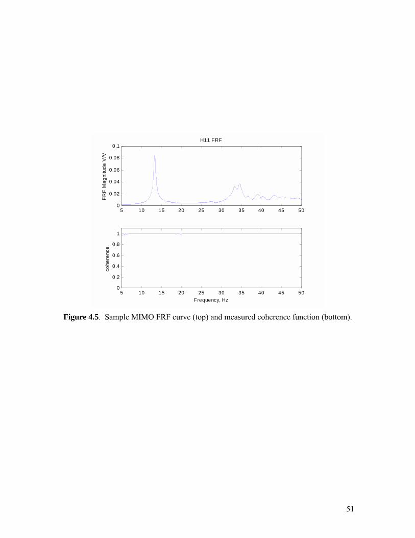
51
5 10 15 20 25 30 35 40 45 500
0.02
0.04
0.06
0.08
0.1H11 FRF
FR
F M
agni
tude
V/V
5 10 15 20 25 30 35 40 45 500
0.2
0.4
0.6
0.8
1
cohe
renc
e
Frequency, Hz
Figure 4.5. Sample MIMO FRF curve (top) and measured coherence function (bottom).
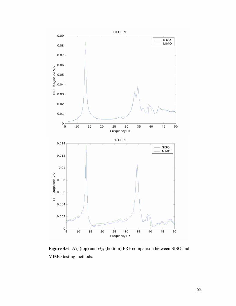
52
5 10 15 20 25 30 35 40 45 500
0.01
0.02
0.03
0.04
0.05
0.06
0.07
0.08
0.09H11 FRF
FR
F M
agni
tude
V/V
Frequency Hz
SISOMIMO
5 10 15 20 25 30 35 40 45 500
0.002
0.004
0.006
0.008
0.01
0.012
0.014H21 FRF
FR
F M
agni
tude
V/V
Frequency Hz
SISOMIMO
Figure 4.6. H11 (top) and H21 (bottom) FRF comparison between SISO and
MIMO testing methods.
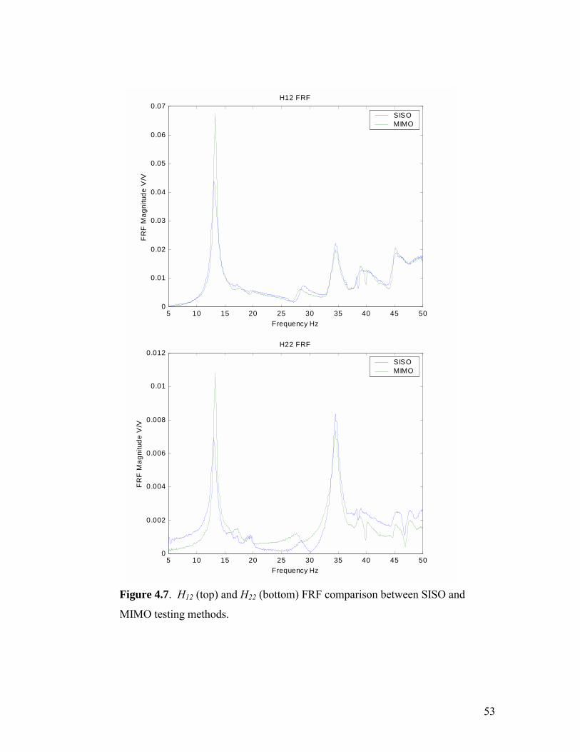
53
5 10 15 20 25 30 35 40 45 500
0.01
0.02
0.03
0.04
0.05
0.06
0.07H12 FRF
FR
F M
agni
tude
V/V
Frequency Hz
SISOMIMO
5 10 15 20 25 30 35 40 45 500
0.002
0.004
0.006
0.008
0.01
0.012H22 FRF
FR
F M
agni
tude
V/V
Frequency Hz
SISOMIMO
Figure 4.7. H12 (top) and H22 (bottom) FRF comparison between SISO and
MIMO testing methods.
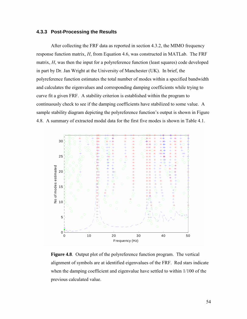
54
4.3.3 Post-Processing the Results
After collecting the FRF data as reported in section 4.3.2, the MIMO frequency
response function matrix, H, from Equation 4.6, was constructed in MATLab. The FRF
matrix, H, was then the input for a polyreference function (least squares) code developed
in part by Dr. Jan Wright at the University of Manchester (UK). In brief, the
polyreference function estimates the total number of modes within a specified bandwidth
and calculates the eigenvalues and corresponding damping coefficients while trying to
curve fit a given FRF. A stability criterion is established within the program to
continuously check to see if the damping coefficients have stabilized to some value. A
sample stability diagram depicting the polyreference functions output is shown in Figure
4.8. A summary of extracted modal data for the first five modes is shown in Table 4.1.
0 10 20 30 40 500
5
10
15
20
25
30
Frequency (Hz)
No
of m
odes
est
imat
ed
Figure 4.8. Output plot of the polyreference function program. The vertical
alignment of symbols are at identified eigenvalues of the FRF. Red stars indicate
when the damping coefficient and eigenvalue have settled to within 1/100 of the
previous calculated value.
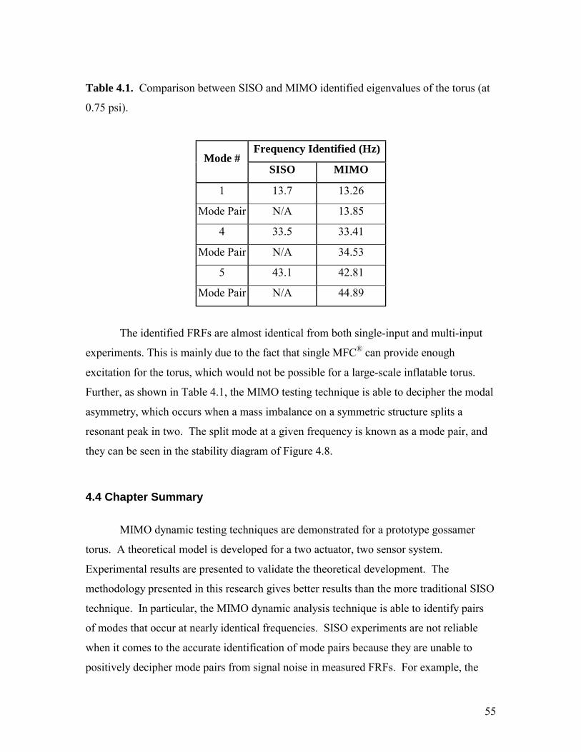
55
Table 4.1. Comparison between SISO and MIMO identified eigenvalues of the torus (at
0.75 psi).
Frequency Identified (Hz) Mode #
SISO MIMO
1 13.7 13.26
Mode Pair N/A 13.85
4 33.5 33.41
Mode Pair N/A 34.53
5 43.1 42.81
Mode Pair N/A 44.89
The identified FRFs are almost identical from both single-input and multi-input
experiments. This is mainly due to the fact that single MFC® can provide enough
excitation for the torus, which would not be possible for a large-scale inflatable torus.
Further, as shown in Table 4.1, the MIMO testing technique is able to decipher the modal
asymmetry, which occurs when a mass imbalance on a symmetric structure splits a
resonant peak in two. The split mode at a given frequency is known as a mode pair, and
they can be seen in the stability diagram of Figure 4.8.
4.4 Chapter Summary
MIMO dynamic testing techniques are demonstrated for a prototype gossamer
torus. A theoretical model is developed for a two actuator, two sensor system.
Experimental results are presented to validate the theoretical development. The
methodology presented in this research gives better results than the more traditional SISO
technique. In particular, the MIMO dynamic analysis technique is able to identify pairs
of modes that occur at nearly identical frequencies. SISO experiments are not reliable
when it comes to the accurate identification of mode pairs because they are unable to
positively decipher mode pairs from signal noise in measured FRFs. For example, the

56
mode pair at 13.26 and 13.85 Hz was originally interpreted as a single mode at 13.7 Hz
(Table 4.1). Depending on the application, the smearing of mode pairs into single modes
may adversely affect a control algorithm, depending on the algorithms sensitivity to the
identified resonant frequencies of the system. Further, when considering the magnificent
scale of future gossamer satellites, multiple piezoelectric patches like the MFC® actuator
will be necessary for proper control and sensing authority in the global sense of the
structure.
57
CHAPTER 5: Positive Position Feedback Control of a Plate Using an MFC® Sensor 5.1 Introduction
This chapter focuses on the dynamic analysis and active vibration suppression of
a simply supported plate using positive position feedback (PPF) controller and MFC®
actuators and sensors. The goals of performing these experiments are to 1) validate the
methodology developed in Chapter 3, and 2) understand the capabilities of MFC®
actuators/sensors. A successful demonstration of vibration analysis and control of a plate
using these devices can help identify the capabilities and limitations of the MFC®
devices. Once the method is understood and validated for a simple structure, applications
for a more complicated structure, like the inflated torus, will be relatively easier.
An outline of the chapter is as follows. Section 5.2 gives background information
on PPF controller. Section 5.3 discusses the analytical solutions for the natural
frequencies of a simply supported plate and describes the experimental setup for the
modal analysis of the same. Section 5.4 describes the experimental setup for
implementing the PPF controller on the plate and details the experimental results.
Finally, Section 5.5 summarizes the results.
5.2 Background on Positive Position Feedback Control Theory and Implementation
The idea of a PPF controller was first introduced by Goh and Caughey (1985). A
PPF controller, sometimes referred to as a PPF filter, can be understood through a set of
equations describing the interaction between the behavior of the structure as well as the
compensator. Using a PPF controller, vibration of the different modes of a structure can
be targeted individually. The equation governing the vibration of a structure at the nth
mode can be described by the following equation:

58
nn2
nnnnn f2 =++ ξωξωζξ &&& (5.1)
where ξn is the modal coordinate, ωn is the natural frequency, ζn is the modal damping,
and fn is the modal force. The modal force generated by the controller is given by
n2
nnn gf ηω= (5.2)
where gn is a positive scalar gain and η is generated by the controller, which is described
by the following second-order differential equation:
ξωηωηωζη 222ffff =++ &&& (5.3)
In Equation (5.3), ωf and ζf are called the frequency and damping ratio of the PPF
controller. Usually, the controller assumes a higher damping ratio than the damping ratio
of the structure. It can be seen from Equations (5.1) and (5.3) that the controller uses
modal coordinates to obtain η, which is subsequently fed back to the structure. A block
diagram of the PPF controller is shown in Figure 5.1.
∫ ∫
Figure 5.1. A block diagram of a PPF controller.
Fanson and Caughey used pairs of PVDF sensors and actuators to control the
vibration of an aluminum beam using a Positive Position Feedback algorithm (Fanson
ωf2
2ζfωf
ωf2
59
and Caughey, 1987). The authors used ceramic sensors and actuators on a cantilevered
aluminum beam. They also developed a root locus plot to show how the poles of their
system were manipulated with the introduction of a PPF controller. The results of the
authors experiments proved the robustness of the PPF controller. Using just two
collocated sensor / actuator pairs, the authors were able to control the first six modes of
vibration of the structure.
Poh and Baz (1990) developed an extended PPF controller model and called it a
Modal Positive Position Feedback controller. The main difference between the two
control algorithms is that the MPPF controller uses first order filters to achieve similar
controller characteristics as the second-order PPF design. The authors validated their
approach by controlling the second mode of vibration of a flexible truss structure using a
single piezoceramic actuator.
When it comes to gossamer structures, PPF control stands out as a strong
candidate for vibration control. PPF control design features two main benefits when
compared to more traditional feedback control algorithms. First, the PPF controller is
relatively simple to design and implement into a dynamic system. Second, PPF
controllers are rather robust in the presence of parameter uncertainties and improperly
modeled (or unknown) system dynamics. Fanson and Caughey (1987) recognized in
their work that the phenomenon of spillover (the presence of uncontrolled modes within
the bandwidth of the closed loop system) could be avoided by using PPF control because
the filter rolls off at high frequency and doesnt put energy into any of the residual
modes. In addition, is not destabilized by finite actuator dynamics. When looking at
structures as complex as a gossamer torus or strut, parameter uncertainties and
unmodeled system dynamics are the norm. Therefore, PPF control is one possible choice
for the control of these structures and demonstrating its effectiveness will open the
possibility of more advanced control algorithms. Further, the results will help establish a
practical basis for implementing more advanced algorithms with the torus or similar
structures.
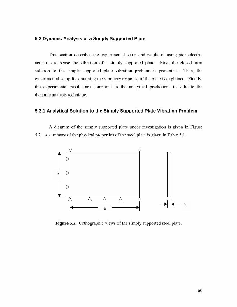
60
5.3 Dynamic Analysis of a Simply Supported Plate
This section describes the experimental setup and results of using piezoelectric
actuators to sense the vibration of a simply supported plate. First, the closed-form
solution to the simply supported plate vibration problem is presented. Then, the
experimental setup for obtaining the vibratory response of the plate is explained. Finally,
the experimental results are compared to the analytical predictions to validate the
dynamic analysis technique.
5.3.1 Analytical Solution to the Simply Supported Plate Vibration Problem
A diagram of the simply supported plate under investigation is given in Figure
5.2. A summary of the physical properties of the steel plate is given in Table 5.1.
Figure 5.2. Orthographic views of the simply supported steel plate.
a
b
h

61
Table 5.1. Summary of the physical properties of the cold-rolled steel plate of
Figure 5.1.
Property Notation Dimension
Length a 0.6 m
Width b 0.5 m
Height h 0.003 m
Elastic Modulus E 190 GPa
Poisson's Ratio v 0.4
Density p 7920 kg/m3
The natural frequencies of the system are given by (Meirovitch, 1992)
hD
bn
am E
mn ρπω
+
=
222 , (5.3)
where
)1(12 2
3
vEhDE −
= . (5.4)
A summary of the first three natural frequencies, as predicted by Equation (5.3), is given
in Table 5.2.
Table 5.2. The first three natural frequencies of the plate.
Natural Frequency # Frequency (Hz)
1 49.3
2 109.9
3 136.5
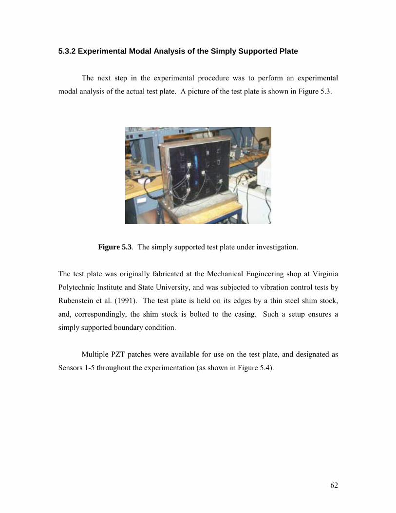
62
5.3.2 Experimental Modal Analysis of the Simply Supported Plate
The next step in the experimental procedure was to perform an experimental
modal analysis of the actual test plate. A picture of the test plate is shown in Figure 5.3.
Figure 5.3. The simply supported test plate under investigation.
The test plate was originally fabricated at the Mechanical Engineering shop at Virginia
Polytechnic Institute and State University, and was subjected to vibration control tests by
Rubenstein et al. (1991). The test plate is held on its edges by a thin steel shim stock,
and, correspondingly, the shim stock is bolted to the casing. Such a setup ensures a
simply supported boundary condition.
Multiple PZT patches were available for use on the test plate, and designated as
Sensors 1-5 throughout the experimentation (as shown in Figure 5.4).
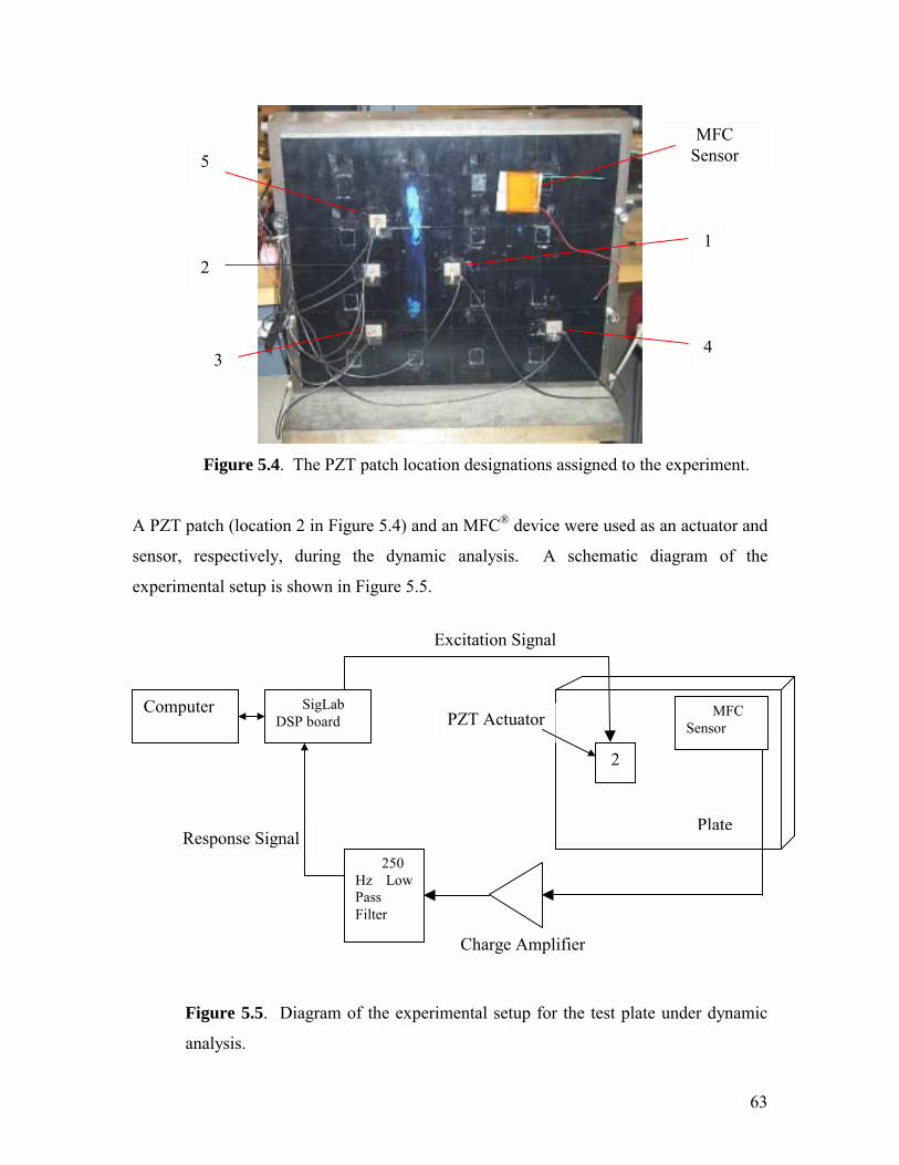
63
Figure 5.4. The PZT patch location designations assigned to the experiment.
A PZT patch (location 2 in Figure 5.4) and an MFC® device were used as an actuator and
sensor, respectively, during the dynamic analysis. A schematic diagram of the
experimental setup is shown in Figure 5.5.
Figure 5.5. Diagram of the experimental setup for the test plate under dynamic
analysis.
5
2
3
1
4
MFC Sensor
Response Signal
Excitation Signal
Computer SigLab DSP board
2
Charge Amplifier
Plate
PZT Actuator MFC Sensor
250 Hz Low Pass Filter
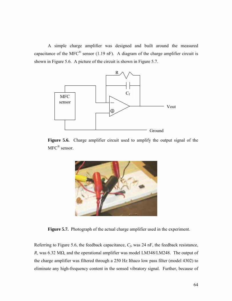
64
A simple charge amplifier was designed and built around the measured
capacitance of the MFC® sensor (1.19 nF). A diagram of the charge amplifier circuit is
shown in Figure 5.6. A picture of the circuit is shown in Figure 5.7.
Figure 5.6. Charge amplifier circuit used to amplify the output signal of the
MFC® sensor.
Figure 5.7. Photograph of the actual charge amplifier used in the experiment.
Referring to Figure 5.6, the feedback capacitance, Cf, was 24 nF, the feedback resistance,
R, was 6.32 MΩ, and the operational amplifier was model LM348/LM248. The output of
the charge amplifier was filtered through a 250 Hz Ithaco low pass filter (model 4302) to
eliminate any high-frequency content in the sensed vibratory signal. Further, because of
R
Cf MFC sensor
Ground
Vout
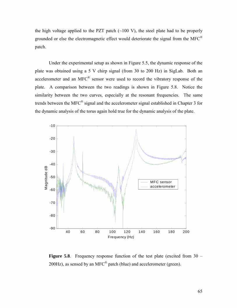
65
the high voltage applied to the PZT patch (~100 V), the steel plate had to be properly
grounded or else the electromagnetic effect would deteriorate the signal from the MFC®
patch.
Under the experimental setup as shown in Figure 5.5, the dynamic response of the
plate was obtained using a 5 V chirp signal (from 30 to 200 Hz) in SigLab. Both an
accelerometer and an MFC® sensor were used to record the vibratory response of the
plate. A comparison between the two readings is shown in Figure 5.8. Notice the
similarity between the two curves, especially at the resonant frequencies. The same
trends between the MFC® signal and the accelerometer signal established in Chapter 3 for
the dynamic analysis of the torus again hold true for the dynamic analysis of the plate.
40 60 80 100 120 140 160 180 200-90
-80
-70
-60
-50
-40
-30
-20
-10
Frequency (Hz)
Mag
nitu
de d
B
MFC sensor accelerometer
Figure 5.8. Frequency response function of the test plate (excited from 30
200Hz), as sensed by an MFC® patch (blue) and accelerometer (green).
66
A comparison between the experimentally determined resonant frequencies and the
analytically determined resonant frequencies of the simply supported plate is given in
Table 5.3.
Table 5.3. Comparison between the analytically and experimentally determined
resonant frequencies of the simply supported plate.
Identified Resonant Frequency (Hz) Mode #
Analytical Experimental
Analytical - Experimental %
Deviation
1 49.3 49.0 0.61
2 109.9 108.0 1.73
3 136.5 132.8 2.71
As shown in Table 5.3, there is less than 3% deviation between the experimental and
analytical resonant frequencies. The superior sensing capabilities of the MFC® device
were further evidenced by the dynamic analysis experiment. After determining the
natural frequencies of the test plate using PZT patches and the MFC® sensor, the next
step is to control its first mode of vibration using a PPF controller.
5.4 Vibration Control of a Simply Supported Plate Using a PPF Controller
Cole (1992) designed a single input, multiple output LQG control technique to
actively reduce the vibration of a simply supported plate. Cole used one of five PZT
actuators (1.2 x 1.0) and sixteen PZT sensors (1.0 x 1.1) in the experiment. The
actuators were placed at the antinodes of the plates first five modes. The sensors were
organized in a grid fashion on the face of the plate. The SIMO LQG controller attacked
the modes of the plate that fell below 200 Hz due to limitations in the data acquisition
system used. In Coles experiment, a 1 V signal was applied to a single PZT actuator to
act as the system disturbance, and a single actuator was used to implement the control
law. However, the control algorithm could only reduce the vibration of the test plate by
67
50% (with an applied control voltage of 2.5 V) when attacking the algorithms most
effective resonant frequency.
Although less complicated in design than a MIMO LQG controller, a PPF
controller will be designed and implemented on the test plate to attack the first mode of
vibration. In the design of a PPF controller, only three compensator parameters need to
be determinedthe compensator gain, g, filter frequency, ωf, and the filter damping
ratio, ζf. McEver (1999) proposed an optimal placement method for these parameters as a
function of the system pole/zero spacing. He found that the amount of damping that
could be added to the closed-loop system by the PPF filter could reach approximately
80% critical damping for high gains. Following McEvers procedure, a filter frequency
of ωω 2≈f was chosen as a starting point throughout the experimentation.
The first mode of the simply supported plate is at 49.0 Hz. Since the piston mode
generates the greatest amount of displacement at the center of the plate, the MFC® sensor
was collocated with the PZT actuator near the center. The MFC® sensor was fastened to
the plate using an epoxy to help limit the loss of energy between the vibration of the plate
and the charge generated by the MFC® device. The output of the MFC® patch was fed
into the charge amplifier, and the amplified signal was fed into the digital PPF controller
through a dSPACE board. The output of the PPF controller was fed into a power
amplifier (50x), and the final control signal was fed back to Patch 1 from Figure 5.4.
Similar to the dynamic analysis experiment in section 5.3, a 5 V chirp signal was used to
excite the structure from 30 200 Hz. A diagram of the experimental setup is shown in
Figure 5.9.
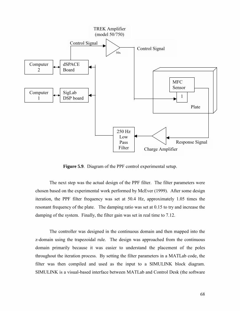
68
Figure 5.9. Diagram of the PPF control experimental setup.
The next step was the actual design of the PPF filter. The filter parameters were
chosen based on the experimental work performed by McEver (1999). After some design
iteration, the PPF filter frequency was set at 50.4 Hz, approximately 1.05 times the
resonant frequency of the plate. The damping ratio was set at 0.15 to try and increase the
damping of the system. Finally, the filter gain was set in real time to 7.12.
The controller was designed in the continuous domain and then mapped into the
z-domain using the trapezoidal rule. The design was approached from the continuous
domain primarily because it was easier to understand the placement of the poles
throughout the iteration process. By setting the filter parameters in a MATLab code, the
filter was then compiled and used as the input to a SIMULINK block diagram.
SIMULINK is a visual-based interface between MATLab and Control Desk (the software
50x
TREK Amplifier (model 50/750)
Control Signal
Response Signal
Control Signal
Computer 1
SigLab DSP board 1
Plate
MFC Sensor
Computer 2
dSPACE Board
Charge Amplifier
250 Hz Low Pass Filter
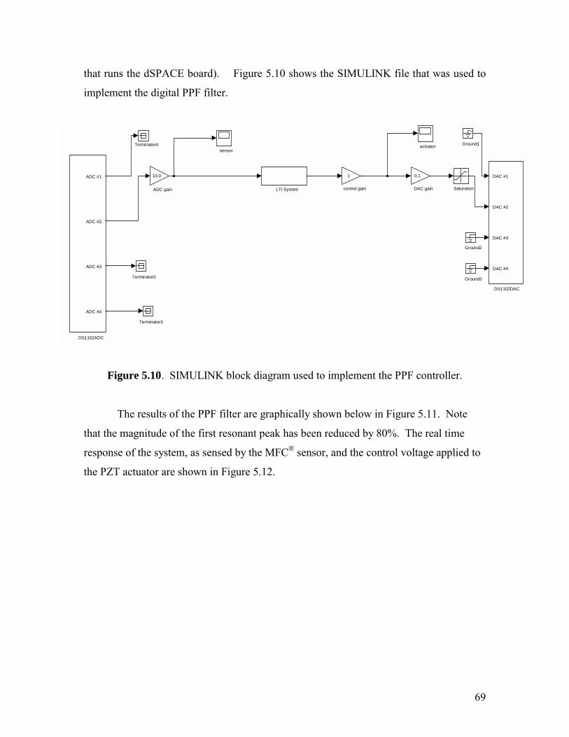
69
that runs the dSPACE board). Figure 5.10 shows the SIMULINK file that was used to
implement the digital PPF filter.
Figure 5.10. SIMULINK block diagram used to implement the PPF controller.
The results of the PPF filter are graphically shown below in Figure 5.11. Note
that the magnitude of the first resonant peak has been reduced by 80%. The real time
response of the system, as sensed by the MFC® sensor, and the control voltage applied to
the PZT actuator are shown in Figure 5.12.
sensor
1 control gain
actuator
Terminator5
Terminator4
Terminator3
Saturation LTI System
Ground3
Ground2
Ground1
DAC #1
DAC #2
DAC #3
DAC #4 DS1102DAC
ADC #1
ADC #2
ADC #3
ADC #4
DS1102ADC
0.1 DAC gain
10.0 ADC gain
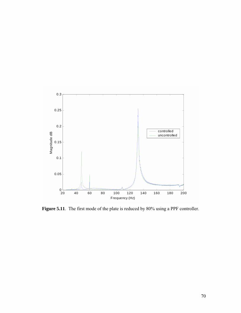
70
20 40 60 80 100 120 140 160 180 2000
0.05
0.1
0.15
0.2
0.25
0.3
Frequency (Hz)
Mag
nitu
de d
B controlled uncontrolled
Figure 5.11. The first mode of the plate is reduced by 80% using a PPF controller.
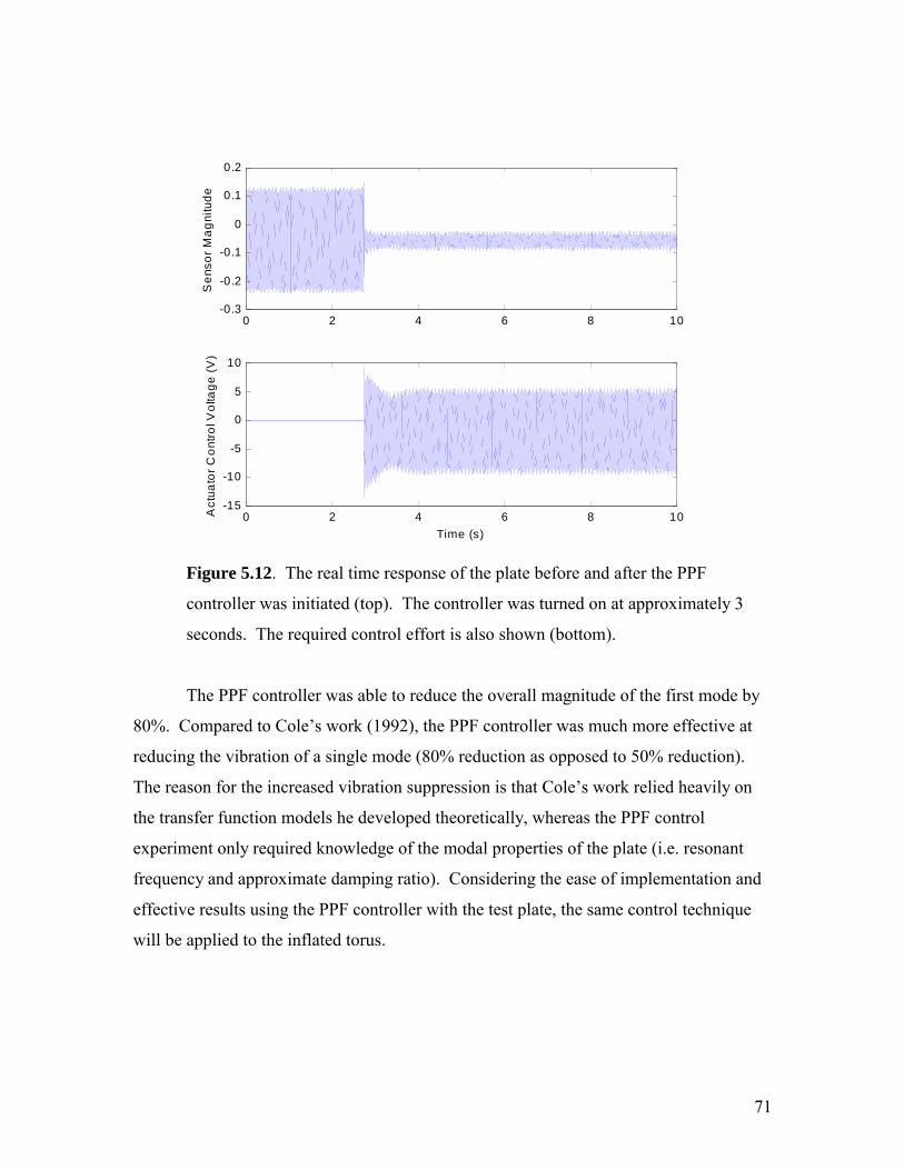
71
0 2 4 6 8 10-0.3
-0.2
-0.1
0
0.1
0.2
Sen
sor M
agni
tude
0 2 4 6 8 10-15
-10
-5
0
5
10
Act
uato
r Con
trol V
olta
ge (V
)
Time (s)
Figure 5.12. The real time response of the plate before and after the PPF
controller was initiated (top). The controller was turned on at approximately 3
seconds. The required control effort is also shown (bottom).
The PPF controller was able to reduce the overall magnitude of the first mode by
80%. Compared to Coles work (1992), the PPF controller was much more effective at
reducing the vibration of a single mode (80% reduction as opposed to 50% reduction).
The reason for the increased vibration suppression is that Coles work relied heavily on
the transfer function models he developed theoretically, whereas the PPF control
experiment only required knowledge of the modal properties of the plate (i.e. resonant
frequency and approximate damping ratio). Considering the ease of implementation and
effective results using the PPF controller with the test plate, the same control technique
will be applied to the inflated torus.

72
5.5 Chapter Summary
A dynamic analysis of a simply supported plate is presented using similar
experimental modal analysis techniques as those developed in Chapter 3. In the latter
half of the chapter, a digital PPF controller was designed and implemented to the control
the first mode of vibration of a simply supported plate. The goal of the research
presented in this chapter was two-fold: 1) to validate the dynamic analysis methodology
developed in Chapter 3, and 2) to demonstrate the effectiveness of using the MFC®
device as a sensor. The PPF controller designed around the MFC® sensor was able to
reduce the magnitude of the vibration levels of the first mode of the plate by nearly 80%
with a maximum control effort of 10V. The next chapter will evaluate the feasibility of
using the PPF active control techniques developed in this chapter to attack the first mode
of vibration of the gossamer torus.
73
CHAPTER 6: Comparison Between Active and Passive Control Techniques for an Inflatable Torus
6.1 Background
In terms of vibration control of a gossamer torus, two approaches can be
undertakennamely 1) an active control algorithm, or 2) a passive control device.
However, in determining the effectiveness of each method, an analysis must be
performed that compares not only the vibratory reduction, but also the trade-offs
associated with that reduction. In particular, the additional mass or altered boundary
conditions imposed on the structure must be taken into account when evaluating the
effectiveness of a specified method.
An outline of the chapter is as follows. Section 6.2 outlines the experimental
setup of implementing a PPF controller to control the vibration of the first mode of the
torus. Section 6.3 outlines the experimental setup and results of using a viscoelastic tape
to reduce the vibration of the torus. Section 6.4 compares the results of both the active
and passive methods attempted in this experimentation. Finally, section 6.5 summarizes
the significant findings of the chapter.
6.2 Active Control of the Gossamer Torus Using a PPF Controller
The experimental setup consisted of the Kapton torus and three MFC® patches.
As opposed to the plate experiment in Chapter 5, the vibration disturbance, vibration
sensor, and PPF controller were all implemented with MFC® patches. A full MFC®
actuator patch supplied the vibration disturbance, and the PPF controller MFC® actuator
and vibration MFC® sensor were equal halves of a full patch. Such an experimental setup
more closely simulates actual working conditions for a space satellite relying solely on
smart material technology. A photograph of the experimental setup is shown in Figure
6.1. A schematic of the experimental setup is shown in Figure 6.2.
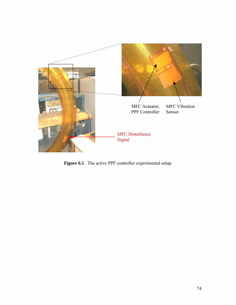
74
Figure 6.1. The active PPF controller experimental setup.
MFC Vibration Sensor
MFC Actuator, PPF Controller
MFC Disturbance Signal
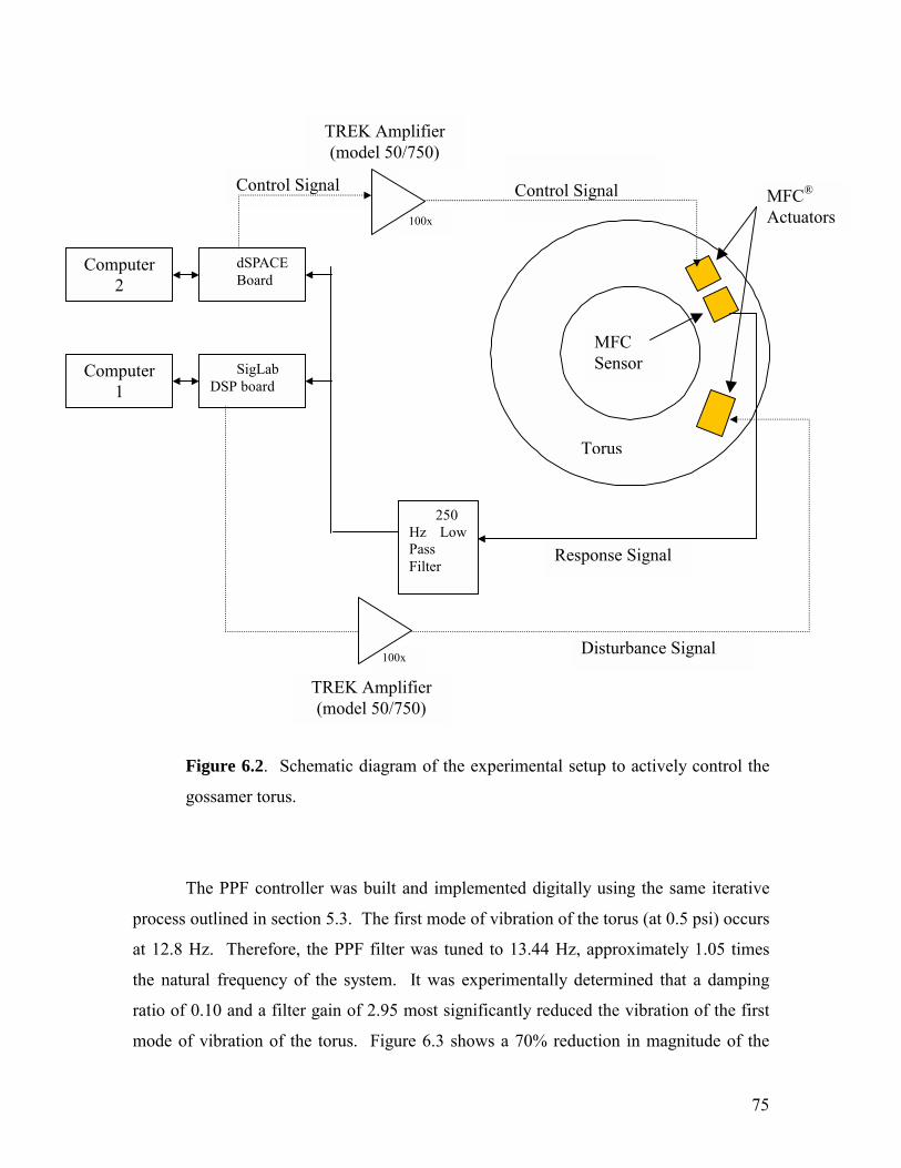
75
Figure 6.2. Schematic diagram of the experimental setup to actively control the
gossamer torus.
The PPF controller was built and implemented digitally using the same iterative
process outlined in section 5.3. The first mode of vibration of the torus (at 0.5 psi) occurs
at 12.8 Hz. Therefore, the PPF filter was tuned to 13.44 Hz, approximately 1.05 times
the natural frequency of the system. It was experimentally determined that a damping
ratio of 0.10 and a filter gain of 2.95 most significantly reduced the vibration of the first
mode of vibration of the torus. Figure 6.3 shows a 70% reduction in magnitude of the
Disturbance Signal
TREK Amplifier (model 50/750)
100x
100x
TREK Amplifier (model 50/750)
Control Signal
Response Signal
Control Signal
Computer 1
SigLab DSP board
Computer 2
dSPACE Board
250 Hz Low Pass Filter
MFC Sensor
MFC® Actuators
Torus
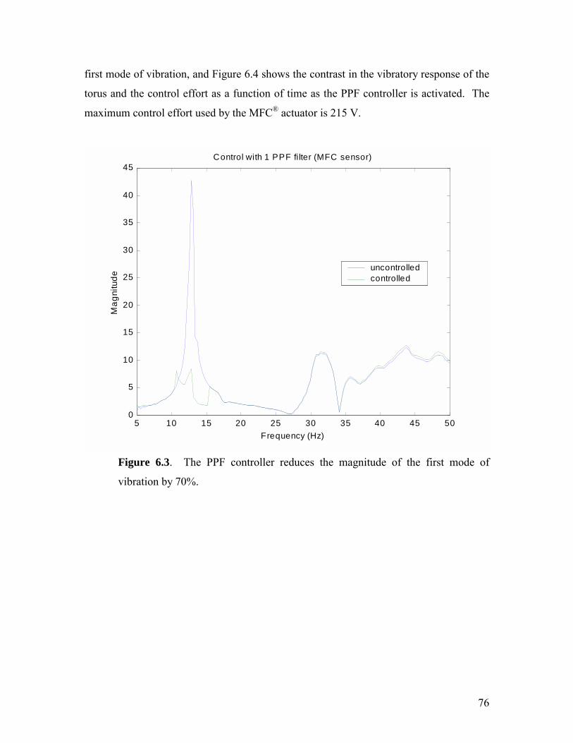
76
first mode of vibration, and Figure 6.4 shows the contrast in the vibratory response of the
torus and the control effort as a function of time as the PPF controller is activated. The
maximum control effort used by the MFC® actuator is 215 V.
5 10 15 20 25 30 35 40 45 500
5
10
15
20
25
30
35
40
45
Frequency (Hz)
Mag
nitu
de
Control with 1 PPF filter (MFC sensor)
uncontrolledcontrolled
Figure 6.3. The PPF controller reduces the magnitude of the first mode of
vibration by 70%.
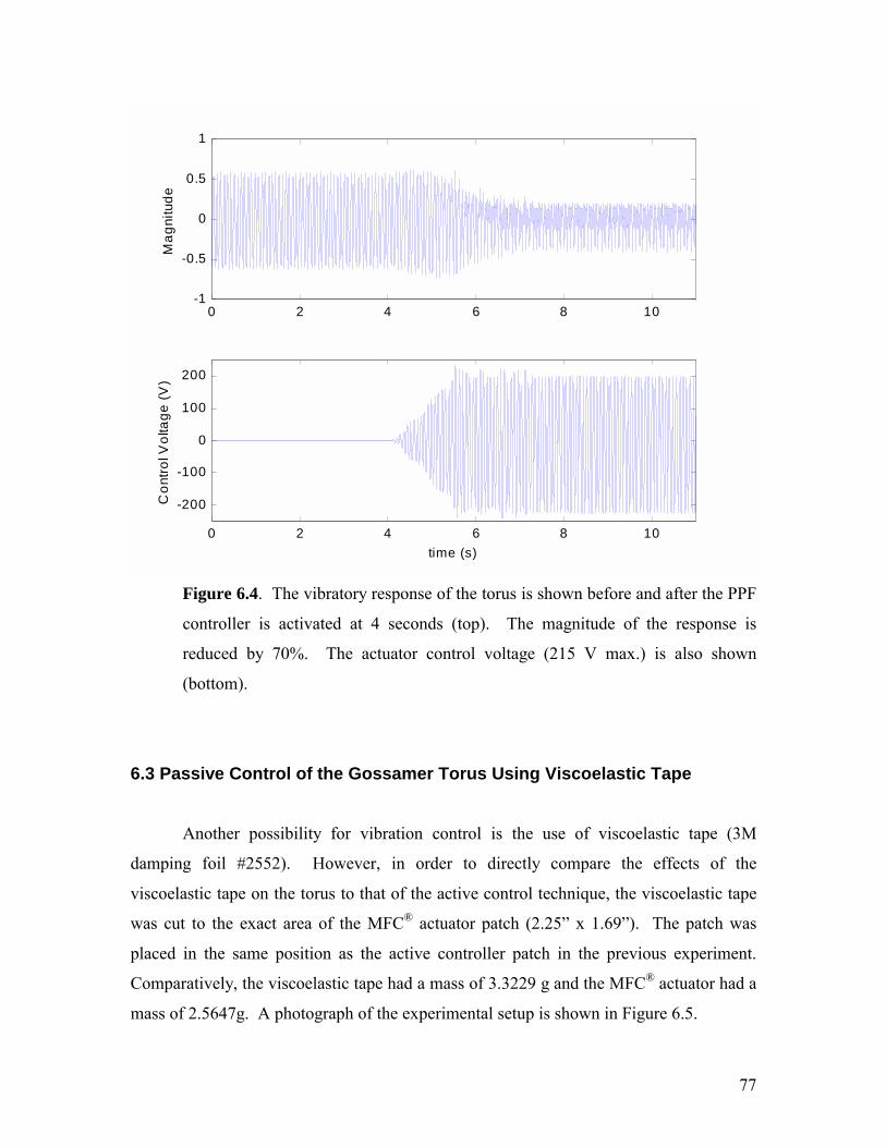
77
0 2 4 6 8 10-1
-0.5
0
0.5
1
Mag
nitu
de
0 2 4 6 8 10
-200
-100
0
100
200
time (s)
Con
trol V
olta
ge (V
)
Figure 6.4. The vibratory response of the torus is shown before and after the PPF
controller is activated at 4 seconds (top). The magnitude of the response is
reduced by 70%. The actuator control voltage (215 V max.) is also shown
(bottom).
6.3 Passive Control of the Gossamer Torus Using Viscoelastic Tape
Another possibility for vibration control is the use of viscoelastic tape (3M
damping foil #2552). However, in order to directly compare the effects of the
viscoelastic tape on the torus to that of the active control technique, the viscoelastic tape
was cut to the exact area of the MFC® actuator patch (2.25 x 1.69). The patch was
placed in the same position as the active controller patch in the previous experiment.
Comparatively, the viscoelastic tape had a mass of 3.3229 g and the MFC® actuator had a
mass of 2.5647g. A photograph of the experimental setup is shown in Figure 6.5.
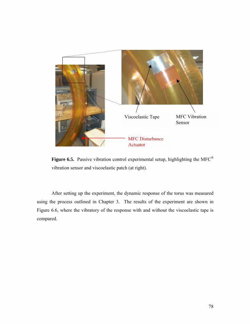
78
Figure 6.5. Passive vibration control experimental setup, highlighting the MFC®
vibration sensor and viscoelastic patch (at right).
After setting up the experiment, the dynamic response of the torus was measured
using the process outlined in Chapter 3. The results of the experiment are shown in
Figure 6.6, where the vibratory of the response with and without the viscoelastic tape is
compared.
MFC Vibration Sensor
Viscoelastic Tape
MFC Disturbance Actuator
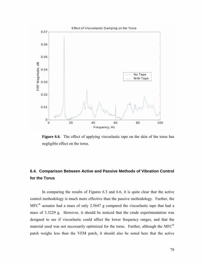
79
0 20 40 60 80 1000
0.01
0.02
0.03
0.04
0.05
0.06
0.07
FR
F M
agni
tude
, dB
F requency, Hz
Effect of V iscoelastic Damping on the Torus
No Tape With Tape
Figure 6.6. The effect of applying viscoelastic tape on the skin of the torus has
negligible effect on the torus.
6.4. Comparison Between Active and Passive Methods of Vibration Control for the Torus
In comparing the results of Figures 6.3 and 6.6, it is quite clear that the active
control methodology is much more effective than the passive methodology. Further, the
MFC® actuator had a mass of only 2.5647 g compared the viscoelastic tape that had a
mass of 3.3229 g. However, it should be noticed that the crude experimentation was
designed to see if viscoelastic could affect the lower frequency ranges, and that the
material used was not necessarily optimized for the torus. Further, although the MFC®
patch weighs less than the VEM patch, it should also be noted here that the active
80
controller requires additional hardware (such as a computer system and power amplifier).
Where the PPF filter was able to reduce the magnitude of the first mode by 70%, the
viscoelastic tape was only able to reduce the magnitude of the first mode by less than 1%.
In addition, the PPF filter was only able to attack the first mode of vibration where the
viscoelastic tape was able to demonstrate some vibration reduction at higher modes (at 47
Hz, 83 Hz, and 89 Hz in Figure 6.6, for example). However, multiple PPF filters can be
tuned so that a single MFC® patch could have control authority over a much larger
bandwidth than the single PPF filter case. For instance, Hegewald (2000) designed
multiple PPF filters to control the vibration of a test plate over a large bandwidth.
6.5 Chapter Summary
A Positive Position Feedback filter was designed and implemented to control the
first mode of vibration of the gossamer torus. The controller was implemented on the
skin of the inflated torus using three MFC® patchesone to act as the disturbance input,
one to sense the vibration of the structure, and the final patch to counteract the vibration
of the torus. With a peak control voltage of 215 V, the MFC® patch was able to reduce
the first mode of vibration of the torus by 70%. In the second half of the experiment, the
active controller was removed and replaced with a piece of viscoelastic tape (3M
damping foil #2552). Recording the systems FRF yet again using this passive technique
had negligible effect on the torus dynamic response. Although the VEM experiment was
performed under non-optimal conditions and with limited investigation, the negligible
reduction at lower resonant frequencies is in agreement with general trends in VEM
damping. Comparatively, the MFC® actuator had less mass (neglecting additional
computational or power hardware) than the viscoelastic tape (2.5647 g as opposed to
3.3229 g), further asserting its compatibility with lightweight, inflatable space structures.
Therefore, considering the negligible mass loading effect and boundary conditions
imposed by the active MFC® controller, the MFC® controller is the best candidate for
future control algorithm implementation.
81
Chapter 7: Conclusions and Future Work The topic of this work was the active dynamic analysis and control of a gossamer
torus. Gossamer structures, like the torus, are the building blocks of future space
satellites. Current imaging and communication limitations are governed by the overall
size of the satellite lens or aperture in orbit. By demonstrating means of dynamic
analysis and control of these lightweight structures, this research provides a feasible
means for deploying gossamer satellites into space.
The first aspect of this research was the dynamic analysis of a 6-foot diameter
Kapton torus. The torus was suspended from a single bungee cord to minimize any effect
on the structures behavior and most closely simulate a free-free boundary condition. A
major contribution of this research was the use of smart materials, or more specifically,
piezoelectric materials, as sensing and actuating devices for experimental modal analysis
of gossamer structures. Smart materials are not the final answer to the identification of
the modal parameters of inflatable, gossamer systems. They do, however, possess
lightweight, non-influential characteristics that make them a better choice for system
dynamic characterization.
The structure was excited in two ways in the first set of dynamic analysis
experiments. The first method used an electromagnetic shaker to excite the torus in two
orthogonal directions to obtain the in-plane and out-of-plane mode shapes of the torus. A
PVDF sensor was used to obtain the frequency response function of the torus from 0 to
100 Hz. An accelerometer was also used throughout the experiment to further validate
the results obtained from the PVDF sensor. The first three out-of-plane and first two in-
plane resonant frequencies and corresponding mode shapes were plotted using both the
PVDF sensor acquired data and the accelerometer acquired data. The resonant
frequencies differed by less than 0.4% between each measurement device.
The second method of excitation of the torus was a Macro-fiber Composite
(MFC®) actuator from NASA Langley Research Center. The MFC® actuator provides
82
several advantages compared to traditional piezo-composite materials, including high
strain energy, conformability, and durability. It uses both active and composite
technologies, in addition to inter-digitated electrodes, and offers high performance and
flexibility suitable fur use in inflatable structures. Because of these highly-compatible
gossamer structure characteristics, the MFC® device was used to excite the torus from 0-
200 Hz. Again, a frequency response function was generated using both a PVDF sensor
and an accelerometer, and excellent agreement was found as compared to the original,
more conventional electromagnetic shaker excitation technique.
For the first time in the known literature, the dynamic testing of a gossamer-type
structure was successfully performed using smart materials. Previous attempts at
identifying the frequency response function of an inflatable torus or similar structure had
proven ineffective or produced results with a tremendous amount of uncorrelated content.
Further, the testing methodology outlined is simple to implement and, more importantly,
relatively inexpensive to use. Despite the success of the analysis, there were two major
short falls attributed with the single input single output methodology presented. First, the
technique is unable to distinguish between orthogonal mode pairs located at nearly
identical natural frequencies. Axi-symmetric structures like the torus demonstrate
orthogonal mode pairs that would be identical, ideally, if the torus were perfect, but once
the symmetry is lost, the modes tend to split slightly from each other. SISO techniques
tend to smear the two peaks into one since they are so close to each other in frequency. A
second issue associated with the SISO technique is that it is highly doubtful that a single
MFC® patch will be able to excite a true gossamer spacecraft, like a 25 m in diameter
torus. Although the SISO method was effective in the global sense for the smaller torus,
global excitation becomes an issue for true gossamer satellites.
Because of the two critical issues uncovered from the SISO modal analysis
techniques, a multiple input multiple output technique (MIMO) was investigated on the
torus. However, instead of using PVDF sensors or accelerometers, the test consisted of
multiple MFC® actuators and sensors. For the first time in the known literature, the
MFC® device was used as a sensor. After validating an assumption that the inflated torus
83
behaved linearly over the frequency range of interest, a MIMO post-processing algorithm
was developed. Two sensors and two actuators were used to perform just two
experiments, and from the two experiments, the collected sensory data was processed to
find a matrix transfer function between the input and output of the system. The data was
further processed to identify the resonant frequencies of the torus. The MIMO technique
was able to distinguish the mode pairs and provide a better method of global excitation of
the structure. Therefore, it is highly recommended that future work on modal analysis of
gossamer structures use the MIMO analysis technique identified in this research.
Having established a reliable, effective methodology for the dynamic analysis of a
gossamer structure, the next phase of the experiment was to demonstrate the feasibility of
using active control techniques to control the vibration of the gossamer torus. In the first
half of the control experiment, a Positive Position Feedback controller was designed and
implemented on a simply supported plate. PPF control is a strong candidate for
preliminary control of a gossamer structure because it is relatively simple to design and
practically implement, and it is rather robust in the presence of system uncertainty. The
first experiment was performed on the simply supported plate to ensure that the MFC®
could be used as a sensor in the PPF control feedback loop, as well as to understand the
practical nature of implementing a PPF controller in general. Using a PPF filter to attack
the first mode of vibration of the simply supported plate, the magnitude of the first mode
was reduced by 70%. The PPF control design only required a peak control voltage of 10
V applied to a PZT patch collocated with the MFC® sensor to control the plates
vibration.
In the second phase of the active control experiment, a similar PPF controller was
designed to suppress the first mode of vibration of the torus. The PPF controller was
implemented using MFC® actuators as both the controller and sensor, and the torus was
disturbed using another MFC® actuator. Following the same procedure established to
control the plate, the first mode of vibration of the torus was reduced in magnitude by
70%.
84
As a follow-up experiment, the final phase of experimental control techniques
explored the possibility of using a passive viscoelastic damping material to control the
vibration of the torus. A piece of 3M damping tape (#2552) was cut to cover the same
effective area as the MFC® actuator. Comparatively, the viscoelastic material had a
greater mass than the MFC® actuator (3.3229 g as opposed to 2.5647 g). By taking a
modal analysis of the torus with and without the tape adhered to the torus skin, it was
found that the viscoelastic tape had negligible effect on reducing the vibration of the
torus. The VEM damping experiment, although crude, was able to demonstrate the
inability of the passive technique to affect the lower modes of the torus. In the same
vein, the mass comparison of the MFC® and VEM techniques is not compatible if the
hardware associated with the active controller is taken into account.
PPF control is by no means the ultimate answer to the vibration control of
gossamer structures. The purpose of the active control experiments was to validate a
cost-effective, easily implemented controller and verify that vibration suppression could
be performed on the torus or similar gossamer structures. Having shown the
effectiveness of PPF control, and by establishing a methodology for using smart materials
in the control scheme for gossamer structures, the next step will be to develop more
rigorous, intensive system models and control algorithms. Multivariate or sliding mode
control may be much more aggressive and effective techniques to control the dynamics of
the torus. However, efforts will need to be focused on the accurate system modeling of
the torus or similar gossamer structures. By developing realistic system models, more
rigorous control algorithms can be developed and implemented. Similarly, computational
models of the MFC® actuator / sensor would prove highly valuable in future projects
integrating MFC® technology.
Gossamer technology and related structures have some exciting times ahead.
Once viewed as tenuous and nearly invisible, gossamer technology is slowly coming into
full view of the scientific community. With continual advances in material science,
control algorithms, and energy production, gossamer technology will continue to attract

85
attention. And with the deployment of a 25-meter inflated antenna in outer space before
2010, it will be hard to classify gossamer technology as tenuous anymore.

86
APPENDIX A: MATLab Code The following MATLab code was used to generate the eigenvectors of the torus data (UMPA pseudo least squares method), and to generate the corresponding mode shapes of the torus. (c) S. O'F. Fahey 4-1997 function [Coeff]=forsythe(q,x,w,type); % forsythe.m (c) S. O'F. Fahey 4-1997 % ver 5.2.1997 % % This matlab (tm) function determines the coefficients of Forsythe % orthogonal polymonials, up to order q % % [coeff] = FORSYTHE( q,x,w,'type' ); % % where, q = degree of highest order polynomial, 1 x 1 % x = domain of control variable, n x 1 % w = complex weighting vector on omega, n X p % 'type' = orthogonal condition, % 's' for sum [default], 'v' for vector % Coeff = coefficients of Forsythe polynomials, q x q [s], % and q X pq [v] % % Orthogonal conditions; % sum_i sum_k w_ik' P(x_i)'_j P(x_i)_n w_ik = % 1 if j equals n, else 0 [s] % sum_i w_ik' P(x_i)'_j P(x_i)_n w_ik = % 1 if j equals n, else 0 for every k [v] % for [s], % [Coeff]=[c_q*q] % for [v], % [Coeff]=[ c1_q*q | c2_q*q | ... | cp_q*q] % ****************************************************** check inputs disp(' '); if (exist('type')==1)==0 type=[]; end; if (exist('w')==1)==0 w=ones(size(x,1),1); end; if size(x,2)>1 disp('??? Error using ==> forsythe.m'); disp(' INPUT NOT COLUMN');end; if q>size(x,1)

87
disp('??? Error using ==> forsythe.m'); disp(' INPUT NOT SUFFICIENT SIZE'); end; % ******************************************************************* % ******************************************************************* % ********************************************************** sum loop if isempty(type) | type=='s' | type=='S' % ********************************************************* set up p=zeros(q); normal=zeros(1,q); Ow=ones(1,size(w,2)); for i=1:q XX(:,i)=x.^(i-1); end; %i xx=(x*Ow); % *********************************************** first polynomial p(1:1,1)=[1]; % ********************************************** second polynomial if q>1 XXpw=((XX*p(:,1))*Ow ).*w; an=sum(sum(conj( XXpw ).* ( xx.*XXpw ))); ad=sum(sum(conj( XXpw ).* ( XXpw ))); a(1)=an/ad; p(1:2,2)=[-a(1)*p(1:1,1); 1]; normal(1)=ad; XXpw0=XXpw; end; % ****************************************** remaining polynomials for k=3:q XXpw=((XX*p(:,k-1))*Ow ).*w; an=sum( sum(conj( XXpw ).*( xx.*XXpw))); ad=sum( sum(conj( XXpw ).*( XXpw))); a(k-1)=an/ad; bn=sum( sum(conj( XXpw0 ).*( xx.*XXpw ))); bd=sum( sum(conj( XXpw0 ).*( XXpw0 ))); b(k-2)=bn/bd; p(1:k,k)=[0;p(1:k-1,k-1)]-b(k-2)*[p(1:k,k-2)]-a(k-1)*p(1:k,k-1);
88
normal(k-1)=ad; XXpw0=XXpw; end; %k XXpw=((XX*p(:,q))*Ow ).*w; normal(q)=sum( sum(conj( XXpw ).*( XXpw ))); % ******************************************************************* % ******************************************************************* % ******************************************************* vector loop elseif type=='v' | type=='V' % ********************************************************* set up p=zeros(q,q*size(w,2)); normal=zeros(1,q*size(w,2)); Ow=ones(1,size(w,2)); c=q*[0:size(w,2)-1]; for i=1:q XX(:,i)=x.^(i-1); end; %i xx=(x*Ow); % *********************************************** first polynomial p([1:1],1+c)=ones(1,size(w,2)); % ********************************************** second polynomial if q>1 XXpw=((XX*p(:,1+c)) ).*w; an=sum(conj( XXpw ).* ( xx.*XXpw )); ad=sum(conj( XXpw ).* ( XXpw )); a(1,:)=an./ad; p([1:2],2+c)=[-a(1,:).*p(1:1,1+c); Ow]; normal(1+c)=ad; XXpw0=XXpw; end; % ****************************************** remaining polynomials for k=3:q XXpw=((XX*p(:,k-1+c)) ).*w; an=sum(conj( XXpw ).*( xx.*XXpw)); ad=sum(conj( XXpw ).*( XXpw));

89
a(k-1,:)=an./ad; bn=sum(conj( XXpw0 ).*( xx.*XXpw )); bd=sum(conj( XXpw0 ).*( XXpw0 )); b(k-2,:)=bn./bd; p(1:k,k+c)=[zeros(1,size(w,2));p(1:k-1,k-1+c)]... -(ones(k,1)*b(k-2,:)).*p(1:k,k-2+c)... -(ones(k,1)*a(k-1,:)).*p(1:k,k-1+c); normal(k-1+c)=ad; XXpw0=XXpw; end; %k XXpw=((XX*p(:,q+c)) ).*w; normal(q+c)= sum(conj( XXpw ).*( XXpw )); else disp('??? Error using ==> forsythe.m'); disp(' TYPE INCORRECT'); p=nan; normal=nan; end; %if-elseif-else 's' and 'v' % ********************************************************* normalize Coeff=p./(ones(size(p,1),1)*sqrt(normal));
function [freq,damp,ampl,phas,eigenvalues,eigenvectors,A,B]=opmodal(m,n,omega,h,w); % opmodal.m (c) S. O'F. Fahey 4-1997 % ver 5.2.1997 % % Matlab (TM) Program was written by Sean O'Flaherty Fahey. This code uses an % UMPA pseudo least square method to determine an orthogonal polynomial fit % to complex data with arbitrarily spaced amplitude and frequency information. % % [ freq,damp,ampl,phas,eigenvalues,eigenvectors ] = opmodal( m,n,omega,h,w ) % % where, m = degree of polynomial (num)erator % n = degree of polynomial (denom)inator % [h1 h2 ... hn] = input Xfer columns function to be fit % omega = frequency corresponding to input function % w = weighting vector(s) % % [freq, damp] = resonant frequency and damping % [ampl,phase] = amplitude and phase at resonance % [eigenvalues,eigenvectors] = complex poles and modeshapes

90
% ******************************************************************* set-up j=sqrt(-1); % defines imaginary L=length(omega); % length incoming x-fer to be fit q=max([n+1 m+1]); % max size polynomial % ************************************************************************** % *** Consider H & OMEGA this way to numerically force c.c. results ******** % ************************************************************************** if exist('w')~=1 w=ones(size(h)); disp(' ') disp(' opmodal.m -- no weight') end; H=[conj(h([L:-1:1],:));h]; OMEGA=[-omega(L:-1:1);omega]; w=[w([L:-1:1],:);w]; N_XFER=size(H,2); if size(w,2)~=N_XFER w=w(:,1)*ones(1,N_XFER); disp(' ') disp(' opmodal.m -- even weight applied across spectra') end; % *************************************************************** estimation % *** references; ******* % *** [1] Richardson M., Formenti D.L. "Parameter estimation from FR ******* % *** Meas using RFP", Proc. IMAC, 1982, pp.167-182. ******* % *** [2] Beliveau J.-G., Class notes, CE, UVM, Burlington, VT 05405 ******* % *** [3] Allemang R.J., Brown D.L., Fladung W., Modal Parameter ******* % *** Estimation: UMPA, IMAC 1994, pp.501-514. ******* % ************************************************************************** % ************************************************************************** % *** comments about sources: the large majority of this code is based *****

91
% *** on [1]. [2] gives helpful suggestions and [3] gives an ************** % *** overview of the process ********************************************** % ************************************************************************** % ******************************************************** estimation set-up [Coeff1]=forsythe(m+1,j*OMEGA,w,'v'); [Coeff2]=forsythe(n+1,j*OMEGA,H.*w,'s'); for i=1:q Poly_term(:,i)=(j*OMEGA).^(i-1); end; %i % ************************************************************* mdof spatial X=zeros(N_XFER*(m+1),n);Z=zeros(n,n);G=zeros(N_XFER*(m+1),1); %Y=zeros(N_XFER*(m+1),N_XFER*(m+1));F=zeros(n,1); %<<code checker>> for k=1:N_XFER r=(k-1)*(m+1); P(:,1:m+1)=((w(:,k)*ones(1,m+1)).*Poly_term(:,1:m+1))*Coeff1(1:m+1,r+1:r+(m+1)); T(:,1:n)=( (w(:,k).*H(:,k)) *ones(1,n) ).*( Poly_term(:,1:n+1)*Coeff2(:,1:n) ); W(:,1)=w(:,k).*H(:,k).*( Poly_term(:,1:n+1)*Coeff2(:,n+1) ); X(r+1:r+m+1,1:n)=[-P'*T]; %Y((k-1)*(m+1)+1:k*(m+1),(k-1)*(m+1)+1:k*(m+1))=[P'*P]; %<<code checker, ?==I>> Z=Z+(T'*T); G(r+1:r+m+1,1)=[P'*W]; %F=F-(T'*W); %<<code checker, ?==0>> end; % ****************************************************** parameter estimator B=[[diag(ones(min(size(X)),1))-X'*X]\[-X'*G]]; AA=G-X*B; % ************************************************** parameter normalization B=Coeff2*[B;1]./Coeff2(n+1,n+1); for k=1:N_XFER r=(k-1)*(m+1);

92
A(:,k)=( Coeff1(1:m+1,r+1:r+m+1)*AA(r+1:r+m+1) )./Coeff2(n+1,n+1); end; % ***************************************************** generate output data for k=1:N_XFER [Res(:,k),Pole] = residue(A([m+1:-1:1]',k),B([n+1:-1:1]')); end; %k I=find(imag(Pole)>0); % *********************************************************** output results eigenvalues=Pole(I); damp=sqrt( 1./((imag(eigenvalues)./real(eigenvalues)).^2+1) ); freq=-real(eigenvalues)./damp; eigenvectors=Res(I,:); %recall residues are not \phi_i\phi_j /M ampl=abs(eigenvectors); phas=angle(eigenvectors); A=A;B=B;
function [freq,damp,ampl,phas,eigenvalues,eigenvectors,HH]=vopmodal(m,n,omega,h,w); % vopmodal.m (c) S. O'F. Fahey 4-1997 % ver 5.2.1997 % % Matlab (TM) Program was written by Sean O'Flaherty Fahey. This code uses an % UMPA pseudo least square method to determine an orthogonal polynomial fit to % complex data with arbitrarily spaced amplitude and frequency information. % % [ freq,damp,ampl,phas,eigenvalues,eigenvectors,H ] = vopmodal( m,n,omega,h,w ) % % where, m = degree of polynomial (num)erator % n = degree of polynomial (denom)inator % [h1 h2 ... hn] = input transfer columns functions to be fit % omega = frequency corresponding to input function % w = weighting vector(s) % % [freq, damp] = resonant frequency and damping % [ampl,phase] = amplitude and phase at resonance % [eigenvalues,eigenvectors] = complex poles and modeshapes % [H] = generated transfer functions % % A graphical interface window will appear requiring user input. The minimum % and maximum frequencies to be considered should be clicked.

93
% ******************************************************************* set-up q=max([n+1 m+1]); % max size polynomial N_XFER=size(h,2); if exist('w')~=1 w=ones(size(h)); disp(' ') disp(' vopmodal.m -- no weight') end; % ********************************************************* find reduced set % *** This allows reducing the xfer function visually when it is ********** % *** not desirable to fit the entire range of motion ********************** % ************************************************************************** figure; plot(omega,w);ylabel('weight') %subplot(3,1,1);plot(omega,w);ylabel('weight') figure; plot(omega,angle(h));ylabel('phase') %subplot(3,1,2);plot(omega,angle(h));ylabel('phase') figure;semilogy(omega,abs(h)); xlabel('frequency');ylabel('amplitude'); %subplot(3,1,3);semilogy(omega,abs(h)); xlabel('frequency');ylabel('amplitude'); grip=ginput(2); [junk, l1] = min( abs(omega-min(grip(:,1))) ); [junk, l2] = min( abs(omega-max(grip(:,1))) ); [freq,damp,ampl,phas,values,vectors,A,B]=opmodal(m,n,omega(l1:l2),h(l1:l2,:),w(l1:l2,:)); % ********************************************************** for output plot for i=1:q; Pn(:,i)=(j*omega).^(i-1); end; % ********************************************* regenerate transfer function for k=1:N_XFER HH(:,k)=(Pn(:,1:m+1)*A(:,k))./(Pn(:,1:n+1)*B); end; %k % ************************************************************** plot result clf;figure semilogy(omega,abs(h),'g.',omega,abs(HH),'m-',omega([l1 l2]),abs(h([l1 l2])),'b*'); title(['Fit: m(num)=' num2str(m) ' & n(den)=' num2str(n)]); xlabel('Frequency');ylabel('Amplitude'); figure
94
plot(omega,angle(h),'g.',omega,angle(HH),'m-',omega([l1 l2]),angle(h([l1 l2])),'b*'); ylabel('Phase'); % *********************************************************** output results freq=freq; damp=damp; ampl=ampl'; phas=phas'; eigenvalues=values; eigenvectors=vectors; % *********************************************************** output file fid = fopen('damping.txt','a'); fprintf(fid,'Natural frq. : \t %f \t Zeta : \t %f \t Ampl. : \t %f \n', freq, damp,ampl); fclose(fid);
The following code plots the mode shapes of the torus. %clear all close all nc=12; %number of circles around the torus. A torus lies in x-y plane nsc=36; %number of points (nodal points) around the small circles %(nordal circle) Ro=60; % radius of a torus Ri=10; % radius of a nordal circle theta=[0:nsc]*2*pi/nsc; %Angle between noral points in nordal circles Phi=[0:nc]*2*pi/nc; %Angle between nordal circles %create nordal circles. a nordal circle lies in y-z plane. starts at (y,z)=(0, Ri) %and clockwise. for i=1:nc+1 for j=1:length(theta) eval(['circle',int2str(i),'y(',int2str(j),')=Ri*sin(theta(j));']) eval(['circle',int2str(i),'z(',int2str(j),')=Ri*cos(theta(j));']) eval(['circle',int2str(i),'x(',int2str(j),')=Ri*sin(theta(j))*0;']) end end for i=1:nc+1 % and then orient them according to Phi. Trans=[cos(Phi(i)) sin(Phi(i)) ; -sin(Phi(i)) cos(Phi(i))]; eval(['ocircle',int2str(i),'xy=Trans*[circle',int2str(i),... 'x; circle',int2str(i),'y];']) end

95
%Put each circle into initial torus shapes coordinate. %Starts at (x,y)=(0,Ro) and clockwise RX=Ro*sin(Phi); RY=Ro*cos(Phi); for i=1:nc+1 %put each circle into the original position. eval(['ncircle',int2str(i),'x=transpose(ocircle',int2str(i),'xy(1,:)+RX(',int2str(i),'));']) eval(['ncircle',int2str(i),'y=transpose(ocircle',int2str(i),'xy(2,:)+RY(',int2str(i),'));']) eval(['ncircle',int2str(i),'z=transpose(circle',int2str(i),'z);']) end %create an initial torus shape for i=1:nc+1 eval(['X(:,',int2str(i),')=ncircle',int2str(i),'x;']) eval(['Y(:,',int2str(i),')=ncircle',int2str(i),'y;']) eval(['Z(:,',int2str(i),')=ncircle',int2str(i),'z;']) end figure surf(X,Y,Z) axis square; axis([-60 60 -60 60 -60 60]); view(-10,10) xlabel('x'), ylabel('y'),zlabel('z') title('orginal torus') % Create mode shapes % since the accelerometer masuremnts are obtained from the normal direction of % the nordal circles in y-z plane, the nordal points move like, % (yn,zn)=Ma*(sin(theta), cos(theta)), where Ma is the shape magnitude. % Since this experiment considers z-direction only (out of plane) motion % change the coordinate of z in nordal circels. nmodes=3; %number of modes we want to plot Zi1=[-0.0345 0.0343 0.0693 0.0507 -0.0224 -0.0828 -0.0518 0.0287 0.0925
96
0.0598 -0.0393 -0.0790 -0.0345]; %24 Hz damp = 0.08 Zi1=Zi1./max(abs(Zi1))*10; title1=('1st mode shape (23.96 Hz)'); Zi2=[ 0.2257 0.4133 -0.0624 -0.3983 0.0485 0.5934 0.1621 -0.2379 0.0778 0.4870 0.1094 -0.2134 0.2257]; %53 Hz 0.09 Zi2=Zi2./max(abs(Zi2))*15; title2=('2nd modeshape (52.38 Hz)'); Zi3=[-1.3816 *0.8 0.2763 1.4244 0.4246 -0.1354 0.9344 0.8383 -0.1860 -0.0196 0.4296 -0.4350 -1.7055 -1.3816*0.8]; %16.94 Hz damp=0.0827 Zi3=Zi3./max(abs(Zi3))*10; title3=('3rd modeshape (78.87 Hz)'); Zi4=[-1.0787*0.5 0.4266 -0.6227 -0.1931 0.3553 -0.7060

97
0.7548 -0.5747 -0.0834 0.8087 -0.6785 0.3874 -1.0787 * 0.5]; %25.31 0.0970 Zi4=Zi4./max(abs(Zi4))*10; title4=('4th modeshape (25.31 Hz)'); Zi5=[-0.9529 0.4896 -1.6044 1.4800 0.5779 -1.1432 1.5177 -1.4306 1.1719 -1.1610 1.1908 -0.6865 -0.9529]; %56 0.1034 Zi5=Zi5./max(abs(Zi5))*10; title5=('5th modeshape (56 Hz)'); for k=1:nmodes for i=1:nc+1 % put the magnitude of mode shape at each node for j=1:length(theta) eval(['ncircle',int2str(i),'z(',int2str(j),')=circle',int2str(i),'z(',int2str(j),')+Zi',int2str(k),'(',int2str(i),');']) end eval(['Z',int2str(k),'(:,',int2str(i),')=ncircle',int2str(i),'z;']) end figure eval(['surf(X,Y,Z',int2str(k),')']) axis square; axis([-75 75 -75 75 -75 75]) xlabel('x'), ylabel('y'),zlabel('z'), view(-10,10) eval(['title(title',int2str(k),');']) end

98
The following MATLab code was used throughout the MIMO experimentation. © Jan Wright and Eric Ruggiero % Calculate (2x2) FRF Matrix from Torus Tests - low frequency - LINEARITY CHECK for % results from 2 voltage levels - using combined actuator FRF approach clear all close all f1 = input('Enter lower frequency for plotting '); f2 = input('Enter upper frequency for plotting '); % FRF Matrix constructed from using two 'combined patch' tests [1 1] and [1 -1] % approach similar to Multi-phase Stepped Sine but only uses single chirp output % but switching patch leads to obtain -1 signal % Low voltage level ********************************************************** load 5V_C_1_31.vna SLm -mat f=SLm.fdxvec'; E=SLm.xcmeas(1,2).xfer; F=SLm.xcmeas(1,3).xfer; clear SLm load 5V_D_1_31.vna SLm -mat f=SLm.fdxvec'; G=SLm.xcmeas(1,2).xfer; H=SLm.xcmeas(1,3).xfer; clear SLm df = f(2) - f(1); fp1 = round(f1/df) + 1; fp2 = round(f2/df) + 1; % Correct FRFs for combined patch tests to a classical FRF matrix related to the two separate patches H2(1,1,:)=.5*E(:)+.5*G(:); H2(2,1,:)=.5*F(:)+.5*H(:); H2(1,2,:)=.5*E(:)-.5*G(:); H2(2,2,:)=.5*F(:)-.5*H(:); figure

99
plot(f(fp1:fp2), abs(squeeze(H2(1,1,fp1:fp2))),f(fp1:fp2),abs(squeeze(H2(2,1,fp1:fp2))),... f(fp1:fp2), abs(squeeze(H2(1,2,fp1:fp2))),f(fp1:fp2),abs(squeeze(H2(2,2,fp1:fp2)))); title('FRFs for low voltage level - combined actuator approach') xlabel('Frequency (Hz)') ylabel('FRF Magnitude V/V') % Same but at high voltage level ********************************************** load 10V_C_1_31.vna SLm -mat f=SLm.fdxvec'; Eh=SLm.xcmeas(1,2).xfer; Fh=SLm.xcmeas(1,3).xfer; clear SLm load 10V_D_1_31.vna SLm -mat f=SLm.fdxvec'; Gh=SLm.xcmeas(1,2).xfer; Hh=SLm.xcmeas(1,3).xfer; clear SLm % Correct FRFs for combined patch tests to a classical FRF matrix related to the two separate patches H2h(1,1,:)=.5*Eh(:)+.5*Gh(:); H2h(2,1,:)=.5*Fh(:)+.5*Hh(:); H2h(1,2,:)=.5*Eh(:)-.5*Gh(:); H2h(2,2,:)=.5*Fh(:)-.5*Hh(:); figure plot(f(fp1:fp2), abs(squeeze(H2h(1,1,fp1:fp2))),f(fp1:fp2),abs(squeeze(H2h(2,1,fp1:fp2))),... f(fp1:fp2), abs(squeeze(H2h(1,2,fp1:fp2))),f(fp1:fp2),abs(squeeze(H2h(2,2,fp1:fp2)))); title('FRFs for high voltage level - combined actuator approach') xlabel('Frequency (Hz)') ylabel('FRF Magnitude V/V') % Overlay two sets of FRFs figure subplot 221 plot(f(fp1:fp2),abs(squeeze(H2(1,1,fp1:fp2))),f(fp1:fp2),abs(squeeze(H2h(1,1,fp1:fp2))),'.') title('H11 FRF for low voltage level - combined actuator approach') xlabel('Frequency (Hz)')

100
ylabel('FRF Magnitude V/V') legend('5V','10V') subplot 222 plot(f(fp1:fp2),abs(squeeze(H2(2,1,fp1:fp2))),f(fp1:fp2),abs(squeeze(H2h(2,1,fp1:fp2))),'.') title('H21 FRF for low voltage level - combined actuator approach') xlabel('Frequency (Hz)') ylabel('FRF Magnitude V/V') legend('5V','10V') subplot 223 plot(f(fp1:fp2),abs(squeeze(H2(1,2,fp1:fp2))),f(fp1:fp2),abs(squeeze(H2h(1,2,fp1:fp2))),'.') title('H12 FRF for low voltage level - combined actuator approach') xlabel('Frequency (Hz)') ylabel('FRF Magnitude V/V') legend('5V','10V') subplot 224 plot(f(fp1:fp2),abs(squeeze(H2(2,2,fp1:fp2))),f(fp1:fp2),abs(squeeze(H2h(2,2,fp1:fp2))),'.') title('H22 FRF for low voltage level - combined actuator approach') xlabel('Frequency (Hz)') ylabel('FRF Magnitude V/V') legend('5V','10V') % Plot Nyquist form for FRFs at HIGH Level figure subplot 221 polar(angle(squeeze(H2h(1,1,fp1:fp2))), abs(squeeze(H2h(1,1,fp1:fp2)))), title('H11 polar plot') subplot 222 polar(angle(squeeze(H2h(2,1,fp1:fp2))), abs(squeeze(H2h(1,1,fp1:fp2)))), title('H21 polar plot') subplot 223 polar(angle(squeeze(H2h(1,2,fp1:fp2))), abs(squeeze(H2h(1,1,fp1:fp2)))), title('H12 polar plot') subplot 224 polar(angle(squeeze(H2h(2,2,fp1:fp2))), abs(squeeze(H2h(1,1,fp1:fp2)))), title('H22 polar plot')

101
************************************************************************ The following is the polyreference program written in part by Dr. Jan Wright and Eric Ruggiero. ************************************************************************ % Program torus_poly % Permits analysis of part of frequency range % Calculate impulse response function matrix from FRF matrix % Use LSCE / Polyreference to identify natural frequencies and damping ratios % - where possible notation as per Cooper's paper in MSSP 1990 4(2) pp157-172 % H is FRF matrix / frequency is array of np2+1 frequencies for which FRF is calculated % FRF carried through from torus_frf % freq_est and zeta_est are estimated values returned % - modal_mass_est and psi_est are generated in jan_lsfd % Copy values from torus_frf H=HH; frequency = f; % Expected max no of modes nmodes = input('Enter expected no of modes in analysis '); [r,e,nfreq] = size(H); % number of responses, exciters, frequency points in H fnyq = frequency(nfreq); % Nyquist frequency df = frequency(nfreq)/(nfreq-1); % frequency step in FRF dt = 1/(2*fnyq); % time step in IRF when generated np21 = nfreq; % data point at Nyquist frequency np22 = np21 + 1; % point beyond Nyquist np2 = nfreq - 1; % half number of time points npts = 2 * np2; % number of time points t = (1:npts)*dt; % vector of time values % Calculate sum blocks for H for use in stabilisation diagram if e == 1 H_sum = squeeze(sum(abs(H))); else H_sum = squeeze(sum(sum(abs(H)))); end % Select bandwidth for 'zoom' analysis if desired and reset parameters (add _z)

102
fig1 = figure; plot(frequency, H_sum); iz = input('Enter 0 for baseband and 1 for zoom analysis '); if iz == 0 % base band fnyq_z = fnyq; nfreq_z = nfreq; df_z = df; dt_z = dt; np21_z = np21; np22_z = np22; np2_z = np2; npts_z = npts; freq_z = frequency; H_z = H; if e == 1 H_sum_z = squeeze(sum(abs(H_z))); else H_sum_z = squeeze(sum(sum(abs(H_z)))); end else if iz == 1 % 'zoom' fig1 = figure; plot(frequency, H_sum); f1 = input('Enter lower frequency bound for fitting? '); f2 = input('Enter upper frequency bound for fitting? '); fp1 = round(f1/df) + 1; fp2 = round(f2/df) + 1; fnyq_z = frequency(fp2) - frequency(fp1); % new Nyquist for band limited FRF nfreq_z = fp2 - fp1 + 1; % new no of frequencies for band limited FRF df_z = df; % df unchanged dt_z = 1 / (2*fnyq_z); % new dt for band limited FRF np21_z = nfreq_z; np22_z = np21_z + 1; np2_z = nfreq_z - 1; npts_z = 2 * np2_z; freq_z = zeros(nfreq_z,1); freq_z(1:nfreq_z) = frequency(fp1:fp2);

103
H_z = zeros(r,e,nfreq_z); H_z(:,:,1:nfreq_z) = H(:,:,fp1:fp2); % Set up band limited FRFs % Calculate sum blocks for H_z for use in stabilisation diagram and plot to check if e == 1 H_sum_z = squeeze(sum(abs(H_z))); else H_sum_z = squeeze(sum(sum(abs(H_z)))); end fig2 = figure; plot(freq_z, H_sum_z); pause end end % Calculate inverse FFT stored in h to yield impulse response function IRF - to achieve this % the FRF must be extended to include negative frequency values as conjugates % in reverse order h = zeros(r,e,npts_z); for ie = 1:e; for ir = 1:r; Hstore = squeeze(H_z(ir,ie,:)); % store current FRF in 1D array Hstore_ext = [Hstore(1:np21_z);conj(Hstore(np2_z:-1:2))]; % extend for ifft hstore = ifft(Hstore_ext); % inverse FFT for stored array h(ir,ie,:) = real(hstore); % restore to 3D array of IRFs end end % Choose a number of points from the decay to encompass the bulk of the active region fig2 = figure; plot(real(hstore(1:np2_z))) % plot sample IRF (last one generated) N = input('Enter no of points in decay to be fitted? '); % Loop around for smax - ie all orders of s (no of submatrices) needed for modes_max % and store frequency and damping values for stabilisation diagram - looping on s % is to avoid the duplication of models that occurs when looping around modes is used % s is effectively the model order of the matrix difference equation - with e>1 it is % not possible to identify every single no of modes from 1:modes_max! modes_max = 4 * nmodes; % max no of modes in fit (arbitrary) smax = ceil(modes_max*2/e); % max size of s (depends on e)

104
freq_est_all = zeros(modes_max,smax); zeta_est_all = zeros(modes_max,smax); % Alter 1 to 2 for loop to overcome e=1 problem JRW 30/1/02 - but problem of 'half modes' remains for s = 2:smax % s is order of block polynomial equation s mm = s*e; % model order >= 2*no of modes smodes = floor(mm/2); % no of modes for this s loop s1 = s + 1; se = s*e; Ns = N-s; Y = zeros(Ns*r,e); PHI = zeros(Ns*r,se); THETA = zeros(se,e); % Fill up matrices with blocks consisting of % impulse response function matrices at different time values wait_handle = waitbar(0, 'Generating matrices'); wcount = 1; rcount = 1; for ib = s1:N Y(rcount:rcount+r-1,:) = squeeze(h(:,:,ib)); % fill Y matrix ecount = 1; for jb = 1:s PHI(rcount:rcount+r-1,ecount:ecount+e-1) = h(:,:,ib-jb); % fill PHI matrix ecount = ecount + e; end rcount = rcount + r; wcount = wcount + 1; waitbar(wcount/Ns); end close(wait_handle) % Solve for THETA via Least Squares THETA = PHI\Y; % Set up sparse block Hessenburg matrix from submatrices in THETA A = zeros(se,se); A(:,1:e) = THETA;

105
A(1:(s-1)*e,e+1:se) = eye((s-1)*e); % Solve for estimated frequency and damping values via eigenvalues of A [Vec,Val] = eig(A); L = diag(Val); el = log(L)/dt_z; omegan_z = abs(el); % Add lower frequency limit to frequencies determined prior to calculating damping omegan = omegan_z + 2 * pi * freq_z(1); zeta_est = -real(el)./omegan; freq_est = omegan /(2*pi); [freq_est,index] = sort(freq_est); zeta_est = zeta_est(index); % Store every other value to allow for complex conjugate roots ialt = (1:2:se-1); freq_est = freq_est(ialt); zeta_est = zeta_est(ialt); [freq_est zeta_est] % Store results [no_freq,dummy] = size(freq_est); freq_est_all(1:no_freq,s) = freq_est; zeta_est_all(1:no_freq,s) = zeta_est; end % Call stabplot function torus_stab(freq_z',H_sum_z,freq_est_all,zeta_est_all,modes_max,smax,e,1,5); pause

106
The next program plots the stability diagram from the polyreference program. This program was written in part by Dr. Jan Wright and Eric Ruggiero. function jan_torus(f,FRF,freq,damp,max_modes,nmodels,e,fm,dm); % Plot a stability plot from LSCE data over a range of fitted models % Check for convergence to within given bounds % f is frequency vector, FRF is SISO FRF vector (eg sum FRFs), purely for plotting % freq and damp are matrices of freq and damping results, where % the first m rows of column n hold the values relating to the nth model fitted. % max_modes is the max no of modes in the curve fit % nmodels is the number of different models fitted by LSCE % e is number of exciters % fm and dm are the (percentage) freq and damping bounds (eg 1 and 5) % Plot FRF and initial freq estimates axis([f(1) max(f) 0 max_modes]) FRF = FRF*max_modes/max(FRF); fig2 = figure; plot(f,FRF,'--',freq,1:max_modes,'w.') xlabel('Frequency (Hz)') ylabel('No of modes estimated') hold on zoom on % Stabilization matrix - codes for whether freq or freq + damp are stabilized stab = zeros(size(freq)); % Initial estimates s = 1; m1 = floor(s*e/2); % no of modes for s=1 (first model order fitted) f1 = freq(1:m1,1); d1 = damp(1:m1,1); for k = 1:m1 plot(f1(k),m1,'g.') axis([f(1) max(f) 0 max_modes]) end % Loop for all remaining estimated models for s = 2:nmodels mm = s * e; % model order m = floor(mm/2); % no of modes fitted f2 = freq(1:m,s); d2 = damp(1:m,s);
107
for k = 1:m count(k) = 0; % counter to indicate whether f2 stabilized end % Loop for each result in current vector f1 for j = 1:m1 % Define confidence bands for current frequencies fbl = f1(j)*(1-fm/100); fbu = f1(j)*(1+fm/100); % Loop for each frequency in new vector f2 and compare to f1(j) for k = 1:m % Compare frequencies if f2(k)>fbl & f2(k)<fbu % ie lies in the given freq band count(k) = 1; % flag to show f2 value stabilised and plotted % Compare dampings dbl = d1(j)*(1-dm/100); dbu = d1(j)*(1+dm/100); if d2(k)>dbl & d2(k)<dbu plot(f2(k),m,'r*') axis([f(1) max(f) 0 max_modes]) stab(k,s)=2; % ie stabilized in frequency & damping else plot(f2(k),m,'b+') axis([f(1) max(f) 0 max_modes]) stab(k,s)=1; % ie stabilized in frequency but not damping end end end end % Plot remaining f2 points as not stabilized for k = 1:m if count(k) == 0 plot(f2(k),m,'go') % frequency not stabilized so plot axis([f(1) max(f) 0 max_modes]) end end % Move to next estimated model and update current vector and % remember current no of modes f1 = f2; d1 = d2; m1 = m; end figure(fig2) hold off

108
The following program was used to calculate the coefficients of the PPF filter for both the plate and torus experiments. Simply modify zp and wp depending on the application. clc; clear; % You need to give inputs in the below. %zp=input('Give the value of Damping Ratio of the beam (in percent): '); %wp=input('Give the value of Natural Frequency of the beam in Hz : '); %gg=input('Give the value of Gain (0.01): '); % 0.2 and 7.8 zp=0.15 wp=37.3*1.05 %zp= 0.10 wp=12.9 work best % controller gain %gg=0.03; %old value %gg=.1 % working value wp=wp*2*pi; % computing PPF filter parameters through the tuning equation zf=sqrt((1.02*zp^2)^2/((1.02*zp^2)^2+0.16)); wf=wp/(1.02*sqrt(1-zf*zf)); % building a filter transfer function numc=[wf*wf]; denc=[1 2*zf*wf wf*wf]; sysc=tf(numc,denc); % converting to discrete domain from continuous domain sysd=c2d(sysc,0.001); % obtain transfer function in discrete time [numd,dend,Tss]=tfdata(sysd,'v')
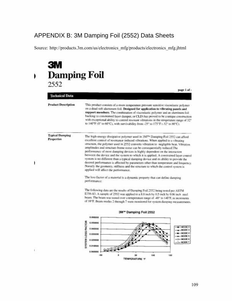
109
APPENDIX B: 3M Damping Foil (2552) Data Sheets Source: http://products.3m.com/us/electronics_mfg/products/electronics_mfg.jhtml
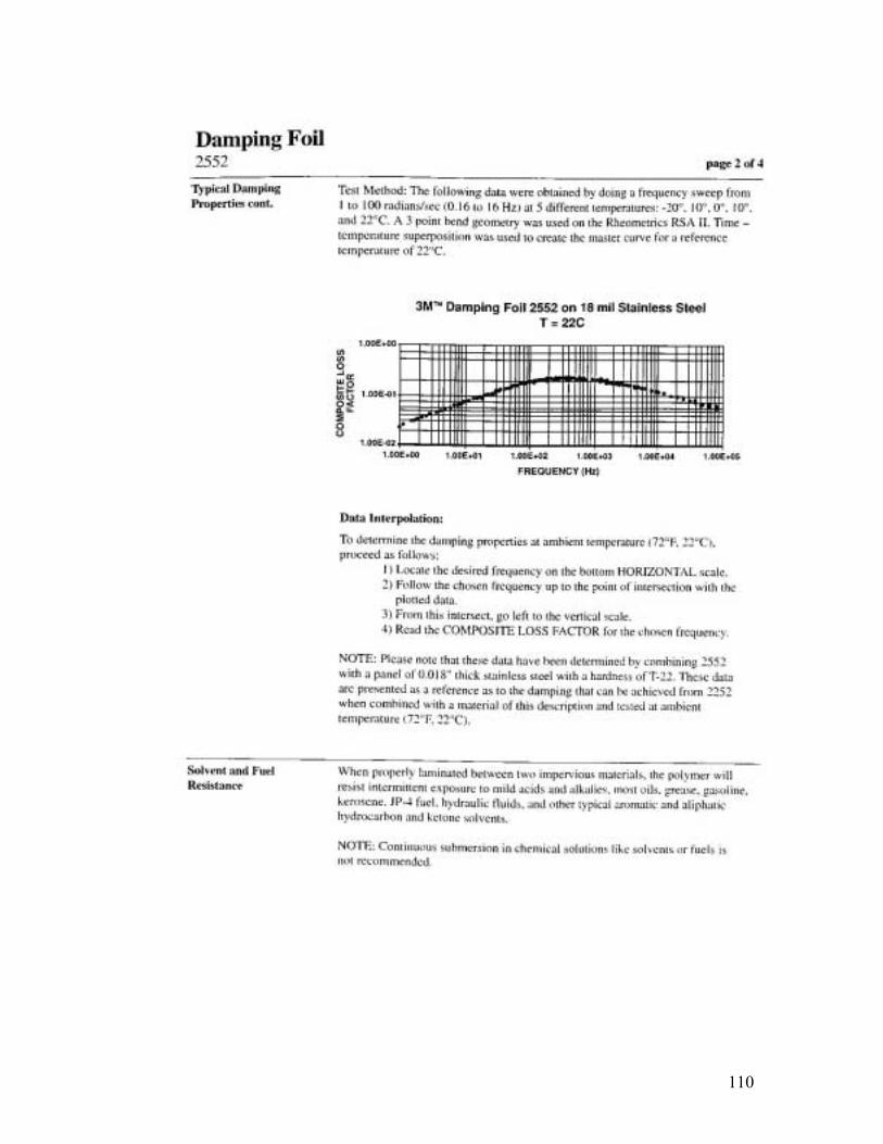
110
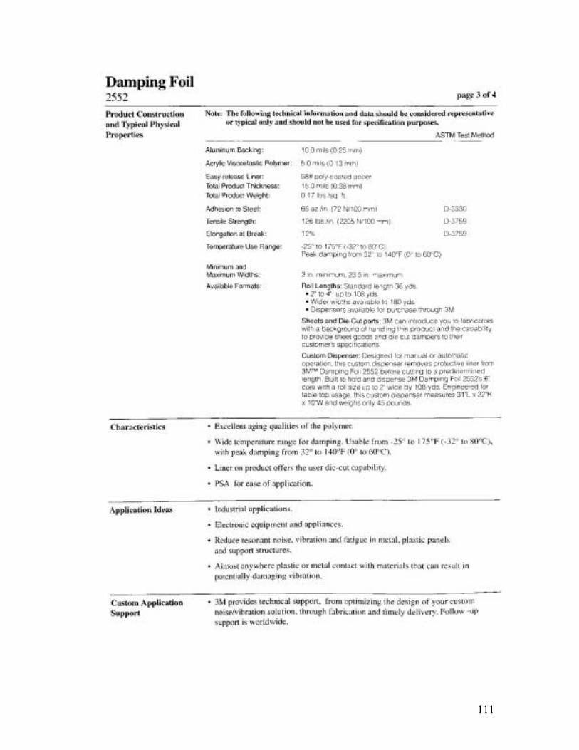
111
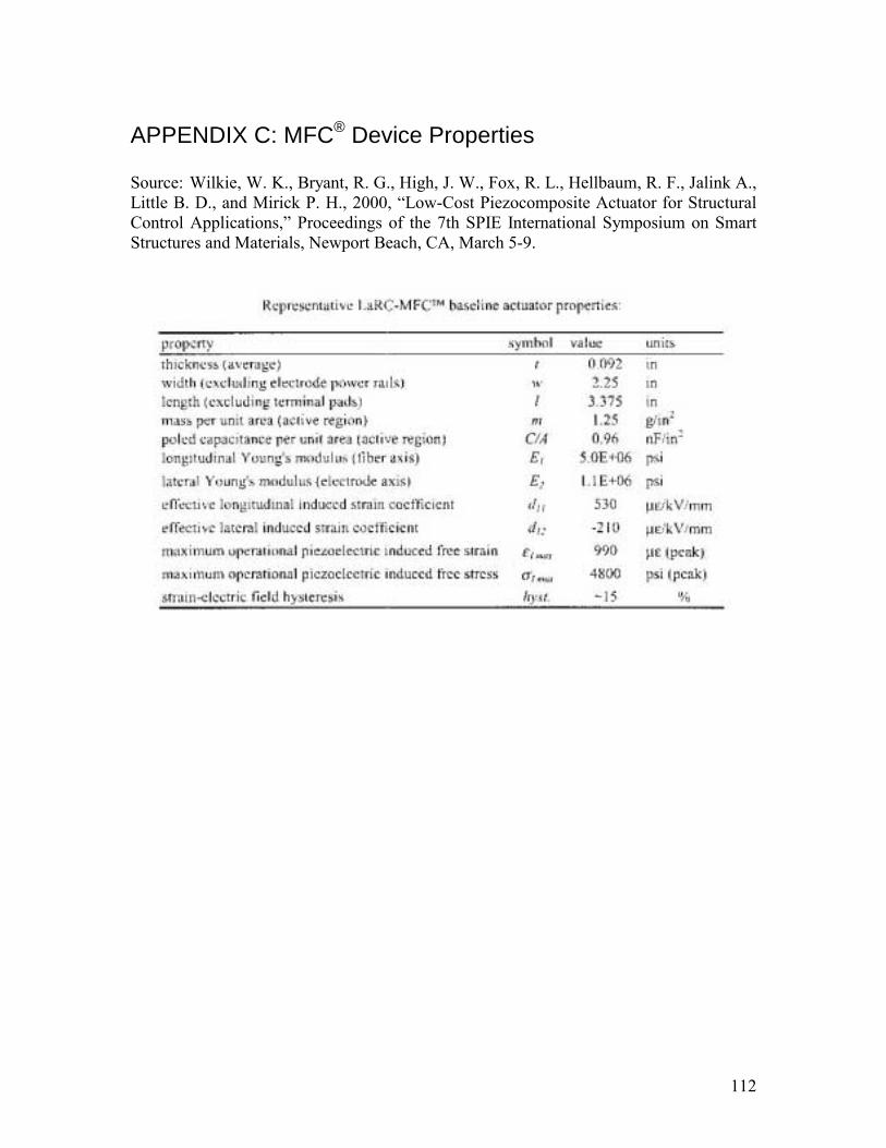
112
APPENDIX C: MFC® Device Properties Source: Wilkie, W. K., Bryant, R. G., High, J. W., Fox, R. L., Hellbaum, R. F., Jalink A., Little B. D., and Mirick P. H., 2000, Low-Cost Piezocomposite Actuator for Structural Control Applications, Proceedings of the 7th SPIE International Symposium on Smart Structures and Materials, Newport Beach, CA, March 5-9.
113
REFERENCES
1. Agnes, G., and Rogers, J. W., 2000, Piezoelectric Excitation of Inflatable Space
Structures for Modal Testing, Proceedings of the 7th Annual Smart Materials and
Structures Conference, International Society for Optical Engineering, SPIE 3985-
88, Newport Beach, CA, pp. 806-816.
2. Allemang, R. J., D. L. Brown, and W. Fladung, 2000, Modal Parameter
Estimation: Unified Matrix Polynomial Approach, Proceedings of the 12th
International Modal Analysis Conference, pp. 501-514.
3. Briand, G., Wicks, A. L., and Inman, D. J., 2000, Vibration Testing for Control
of Inflated Objects, in Proceedings of 18th Annual International Modal Analysis
Conference, pp. 501-514.
4. Chmielewski, A. B., 2000, Overview of Gossamer Technology, Gossamer
Spacecraft: Membrane and Inflatable Structures Technology for Space
Applications, Christopher H. M. Jenkins, ed., AIAA, Vol. 191, pp. 1-33.
5. Chmielewski, A. B., Moore, C., and Howard, R., 1999, The Gossamer
Initiative, IEEE, Paper No. 0-7803-5846-5/00.
6. Clark, S. K., Dodge, R. N., and Nybakken G. H., 1974, Dynamic Properties of
Aircraft Tires, Journal of Aircraft, Vol. 11, No. 3, pp. 166-172.
7. Cole, Daniel G., 1992, Design of, and Initial Experiments with, a MIMO Plate
Control Testbed, MS Thesis, Virginia Polytechnic Institute and State University,
Blacksburg, VA.
8. Dornheim, Michael A., 2000, Inflatable Structures Take to Flight,
http://www.lgarde.com/programs/iaearticle/awarticle.html.
114
9. Dosch, J. J., Inman, D. J., and Garcia, E., 1992, A Self-Sensing Piezoelectric
Actuator for Collocated Control, Journal of Intelligent Material Systems and
Structures, Vol. 3, p. 166.
10. Fanson, J.L. and Caughey, T.K., 1987, "Positive Position Feedback Control for
Large Space Structures", Proceedings of 28th AIAA Structures, Structural
Dynamics and Materials Conference, Monterey, CA, pp. 588-598.
11. Freeland, R. F., 2000, History of Relevant Inflatable High-Precision Space
Structures Technology Developments, Gossamer Spacecraft: Membrane and
Inflatable structures Technology for Space Applications, Christopher H. M.
Jenkins, ed., AIAA, Vol. 191, pp. 33-48.
12. Goh, C. J. and T. K. Caughey, 1985, One the Stability Problem Caused by Finite
Actuator Dynamics in the Collocated Control of Large Space Structures,
International Journal of Control, Vol. 41, pp. 787-802.
13. Griffith, D. T., and Main, J. A., 2000, Modal Testing of an Inflated Thin Film
Polyimide Torus Structure, Proceedings of IMAC XVIII, February, pp. 1035-
1041.
14. Guan, D. H., Yam, L. H., Mignolet, M. P., and Li, Y. Y., 2000, Experimental
Modal Analysis of Tires, Experimental Techniques, November/December, pp.
39-45.
15. Hegewald, Thomas, 2000, Vibration Suppression Using Smart Materials in the
Presence of Temperature Changes, MS Thesis, Virginia Polytechnic Institute and
State University, Blacksburg, VA.

115
16. Leigh, L., Hamidzadeh, H., Tinker, M. L., and Slade, K. N., 2001, Dynamic
Characterization on an Inflatable Concentrator for Solra Thermal Propulsion,
42nd AIAA/ASME/ASCE/AHS/ASC Structures, Structural Dynamics, and
Materials Conference and Exhibit, Seattle, WA, 15-19 March, pp.1-7.
17. Lewis, J. A., 2000, Finite Element Modeling and Active Control of an Inflated
Torus Using Piezoelectric Devices, MS Thesis, Virginia Polytechnic Institute and
State University, Blacksburg, VA.
18. McEver, M. A., 1999, Optimal Vibration Suppression Using On-line Pole/Zero
Identification, MS Thesis, Virginia Polytechnic Institute and State University,
Blacksburg, VA.
19. Noor, A., and Tanner, J., 1985, Advances and Trends in the Development of
Computational Models for Tires, Computers & Structures, Vol. 20, No. 1-3, pp.
517-533.
20. Park, G., Kim, M.-H., and Inman, D. J., 2001, Integration of Smart Materials
into Dynamics and Control of Inflatable Space Structures, Journal of Intelligent
Material Systems and Structures, in press.
21. Poh, S. and A. Baz, 1990, Active Control of a Flexible Structure Using a Modal
Positive Position Feedback Controller, Journal of Intelligent Material Systems
and Structures, Vol. 1, July, pp. 273-288.
22. Rubenstein, S. P., Saunders, W. R., Ellis, Graham K., Robertshaw, H. H., and
Baumann, W. T., 1991, Demonstration of a LQR Vibration Controller for a
Simply-Supported Plate, Recent Advances in Active Control of Sound and
Vibration, Rogers, C. A. and C. R. Fuller, eds., Virginia Polytechnic Institute and
State University, Blacksburg, VA, April 15-17.
116
23. Ruggiero, Eric, Gyuhae Park, Daniel J. Inman, and John A. Main, 2002, Smart
Materials in Inflatable Structure Applications, Proceedings of 43rd
AIAA/ASME/ASCE/AHS/ASC Structures, Structural Dynamics, and Materials
Conference, AIAA Gossamer Spacecraft Forum, April 22-25, Denver, CO.
24. Salama, M., Kuo, C. P., Garba, J., Wada, B., and Thomas, M., 1994, On-Orbit
Shape Correction of Inflatable Structures, AIAA Paper No. 94-1771, pp. 348-
355.
25. Sirohi, J., and Chopra, I., 2000a, Fundamental Behavior of Piezoceramic Sheet
Actuators, Journal of Smart Material Systems and Structures, Vol. 11, January,
pp. 47-61.
26. Sirohi, J., and Chopra, I., 2000b, Fundamental Understanding of Piezoelectric
Strain Sensors, Journal of Smart Material Systems and Structures, Vol. 11,
April, pp. 246-257.
27. Slade, K. N., Tinker, M. L., Lassiter, J. O., and Engberg, R., 2001, Dynamics of
an Inflatable Structure in Vacuum and Ambient Conditions, AIAA Journal, Vol.
39, No. 5, May, pp. 894-901.
28. Sun, F. P., Liang, C., and Rogers, C. A., 1994, Structural Modal Analysis Using
Collocated Piezoelectric Actuator/Sensors an Electromechanical Approach,
SPIE, Vol. 2190, February, pp. 238-249.
29. Sun, F., Rogers, C. A., and Liang, C., 1995, Structural Frequency Response
Function Acquisition via Electric Impedance Measurement of Surface Bonded
Piezoelectric Sensor/Actuator, Proceedings of the 36th AIAA/ASME/ASCE/ASC
Structures, Structural Dynamics, and Materials Conference and AIAA/ASME
Adaptive Structures Forum, Part 5, New Orleans, LA, April, pp. 3450-3458.
117
30. Tinker, M. L., 1998, Passively Adaptive Inflatable Structure for the Shooting
Star Experiment, AIAA Paper No. 98-1986, pp. 2320-2326.
31. Tzou, H.-S., 1998, Multifield Transducers, Devices, Mechatronic Systems, and
Structronic Systems with Smart Materials, The Shock and Vibration Digest, Vol.
30, No. 4, July, pp. 282-294.
32. Wang, B. T., 1998, Structural Modal Testing with Various Actuators and
Sensors, Mechanical Systems and Signal Processing, Vol. 12, No. 5, pp. 627-
639.
33. Wang, B.-T., and Chen, R.-L., 2000, The Use of Piezoceramic Transducers for
Smart Structural Testing, Journal of Smart Material Systems and Structures,
Vol. 11, September, pp. 1-12.
34. Wilkie, W. K., Bryant, R. G., High, J. W., Fox, R. L., Hellbaum, R. F., Jalink A.,
Little B. D., and Mirick P. H., 2000, Low-Cost Piezocomposite Actuator for
Structural Control Applications, Proceedings of the 7th SPIE International
Symposium on Smart Structures and Materials, Newport Beach, CA, March 5-9.
35. Williams, R. B., E. M. Austin, and D. J. Inman, 2001, Limitation of Using
Membrane Theory for Modeling PVDF Patches on Inflatable Structures, Journal
of Intelligent Material Systems and Structures, at press.
36. Yam, L. H., Guan, D. H., and Zhang, A. Q., 2000, Three-dimensional Mode
Shapes of a Tire Using Experimental Modal Analysis, Experimental Mechanics,
Vol. 40, No. 4, December, pp. 369-375.
118
VITA
Eric John Ruggiero
Eric John Ruggiero was born on August 10, 1979 to John and Nancy Ruggiero in
Lawrence, Massachusetts. He graduated valedictorian of the Class of 1997 from Sanborn
Regional High School in Kingston, New Hampshire. In the Fall of 1997, Eric began his
studies in Mechanical Engineering at Virginia Polytechnic Institute and State University
in Blacksburg, Virginia. Throughout his undergraduate career at Virginia Tech, Eric
joined numerous organizations, including Pi Tau Sigma, Tau Beta Pi, the National
Society of Collegiate Scholars, the American Society of Mechanical Engineers, and the
National Society of Professional Engineers. He was also very involved in campus
ministry through the Newman Community Catholic Campus Ministry organization.
From 1999-2000, Eric served as a student campus minister for the Newman Community.
During his tenure as student campus minister, Eric helped organize the communitys 75th
anniversary celebration and traveled to Oaxaca, Mexico to live and work with the poor.
As an undergraduate, Eric used his summers to intern with different companies
and to learn more about the working world. In 1999, he worked at Osram Sylvania in
Hillsborough, New Hampshire as a product development engineer. In 2000 and 2001,
Eric worked at Raytheon Systems Company in Andover, Massachusetts as a
manufacturing engineer. In particular, Eric worked in the circuit card assembly division
responsible for such defense contracts as the Patriot missile, Tomahawk missile, Javelin
weapons system, and many others.
Eric was the recipient of many scholarships and awards during his undergraduate
career at Virginia Tech. Some of the awards he received included the Marshall Hahn
Engineering Scholarship, Seay Scholarship, Faculty honors Scholarship, Litton Industries
Scholarship, Hal L. Moses Scholarship, and the Shorb Award, awarded to a Mechanical
Engineering senior for outstanding leadership and contribution to the field of engineering.
119
Further, Eric was also the recipient of Virginia Techs most prestigious undergraduate
award, the Virginia Tech Man of the Year in 2001. In competition with the entire
University community, Eric received the award based on his demonstration of the ideals
upon which the University is founded uponut prosim.
Eric was accepted into the 5 year MS / BS program in Mechanical Engineering at
Virginia Tech in 2000, and began preliminary research for his advisor, Dr. Daniel J.
Inman, in the Spring of 2001. He performed research on identifying the dynamic
characteristics of an inflated torus, and used this research as the premise for the
remainder of his thesis work.
In August of 2001, Eric married Jennifer L. Vercoe of Colchester, Vermont. The
couple moved to Blacksburg, Virginia so Eric could continue his Masters research and
for Jennifer to teach 1st grade at Falling Branch Elementary in Christiansburg, Virginia.
Eric concluded his Masters research in two semesters after numerous conference paper
and journal paper publications and presentations. Eric capped off his Masters research by
receiving the prestigious Paul E. Torgersen Research Excellence Award, an award given
to the top Masters student who demonstrates both excellence in research as well as
significant contributions to the field of engineering.
Eric and Jennifer currently reside in Blacksburg, Virginia. Eric and his wife will
be traveling to Phoenix, Arizona this summer to see the countryside and to work for
Honeywell Space Systems. Eric will be returning to Virginia Tech in the Fall to continue
his graduate education and earn his Ph.D. in Mechanical Engineering.