1

EECS 452, Winter 2008

Active Noise Cancellation Project Kuang-Hung liu, Liang-Chieh Chen, Timothy Ma, Gowtham Bellala, Kifung Chu 4/17/08

2

Contents

1. Introduction 1.1 Basic Concepts 1.2 Motivations 1.3 Applications 1.4 Programming Environments 1.5 Tools 1.6 Budget

2. Layout 2.1 Adaptive Filter Framework 2.2 Challenges 2.3 MATLAB Example 2.4 Basic outline of LMS and its variations 3. Approach 1: off-line estimation of S(z) 3.1 FxLMS Algorithm 3.2 FuLMS Algorithm 3.3 Feedback ANC 3.4 Hybrid ANC 3.5 Comparison 4. Approach 2 4.1 Input/Output hardware interface. 4.2 Adaptive algorithm 4.3 Sampling rate and filter size design constraint. 4.4 Incorporate music source 5. Experimental Results 6. Future Work 7. Conclusions 8. References

3

1. Introduction Active Noise Cancellation (ANC) is a method for reducing undesired noise. ANC is achieved by introducing a canceling “antinoise” wave through secondary sources. These secondary sources are interconnected through an electronic system using a specific signal processing algorithm for the particular cancellation scheme. Our project is to build a Noise-cancelling headphone by means of active noise control. Essentially, this involves using a microphone, placed near the ear, and electronic circuitry which generates an "antinoise" sound wave with the opposite polarity of the sound wave arriving at the microphone. This results in destructive interference, which cancels out the noise within the enclosed volume of the headphone. This report will demonstrate the approaches that we take on tackling the noise cancellation effects, along with results comparison. 1.1 Basic Concepts Noise Cancellation makes use of the notion of destructive interference. When two sinusoidal waves superimpose, the resulting waveform depends on the frequency amplitude and relative phase of the two waves. If the original wave and the inverse of the original wave encounter at a junction at the same time, total cancellation occur. The challenges are to identify the original signal and generate the inverse without delay in all directions where noises interact and superimpose. We will demonstrate the solutions later in the report.

Figure 1: Signal Cancellation of two waves 180° out of phase.

1.2 Motivations The traditional approach to acoustic noise control uses passive techniques such as enclosures, barriers, and silencers to attenuate the undesired noise. These passive silencers are valued for their high attenuation over a broad frequency range; however, they are relatively large, costly, and ineffective at low frequencies. On the other hand, the ANC system efficiently attenuates low-frequency noise where passive methods are either ineffective or tend to be very expensive or

4

bulky. Most importantly, ANC can block selectively. ANC is developing rapidly because it permits improvements in noise control, often with potential benefits in size, weight, volume, and cost. Blocking low frequency has the priority since most real life noises are below 1 KHz, for example engine noise or noise from aircrafts. This mainly led us to focus our project on low frequency noise cancellation. 1.3 Applications There are a number of great applications for active noise cancellation devices. Noise cancellation almost requires the sound to be cancelled at a source, such as from a loud speaker. That is why the effect works well with headsets, since you can contain the original sound and the canceling sound in an area near your ear. One obvious application is that people working near aircraft or in noisy factories can now wear these electronic noise cancellation headsets to protect their hearing. ANC is ideal for industrial use. The application of active noise reduction produced by engines has various benefits -- the operation of the engines is more convenient for personnel; Noise reduction eliminates vibrations that cause material wearout and increased fuel consumption; Quieting of submarines. The concepts of noise cancellation have abundant applications; these are just to name a few. 1.4 Programming Environments Most of our programming was done in C using Code Composer Studio and VHDL, together with the aid of MATLAB simulations. 1.5 Tools The only external resources that we brought are the headset, and a circuit board for D/A, A/D interfaces. Other instruments that we needed for our project were available in lab. Below is a list of the hardware we used:

• TI TMS320VC5510DSK • Spartan-3 starter board • Microphones Cartridge 6MM OMNI • KOSS Stereo Headset KHP/21V • Maxell Noise Cancellation Headphone

5

1.6 Budget Excluding the lab instruments provided, the cost of our project is kept inexpensive.

Tool Price

Microphones (2 pairs) $ 11.38

Koss Stereo Headset $ 19.97

Maxell Noise Cancellation Headset $ 50.00

TOTAL $ 81.35

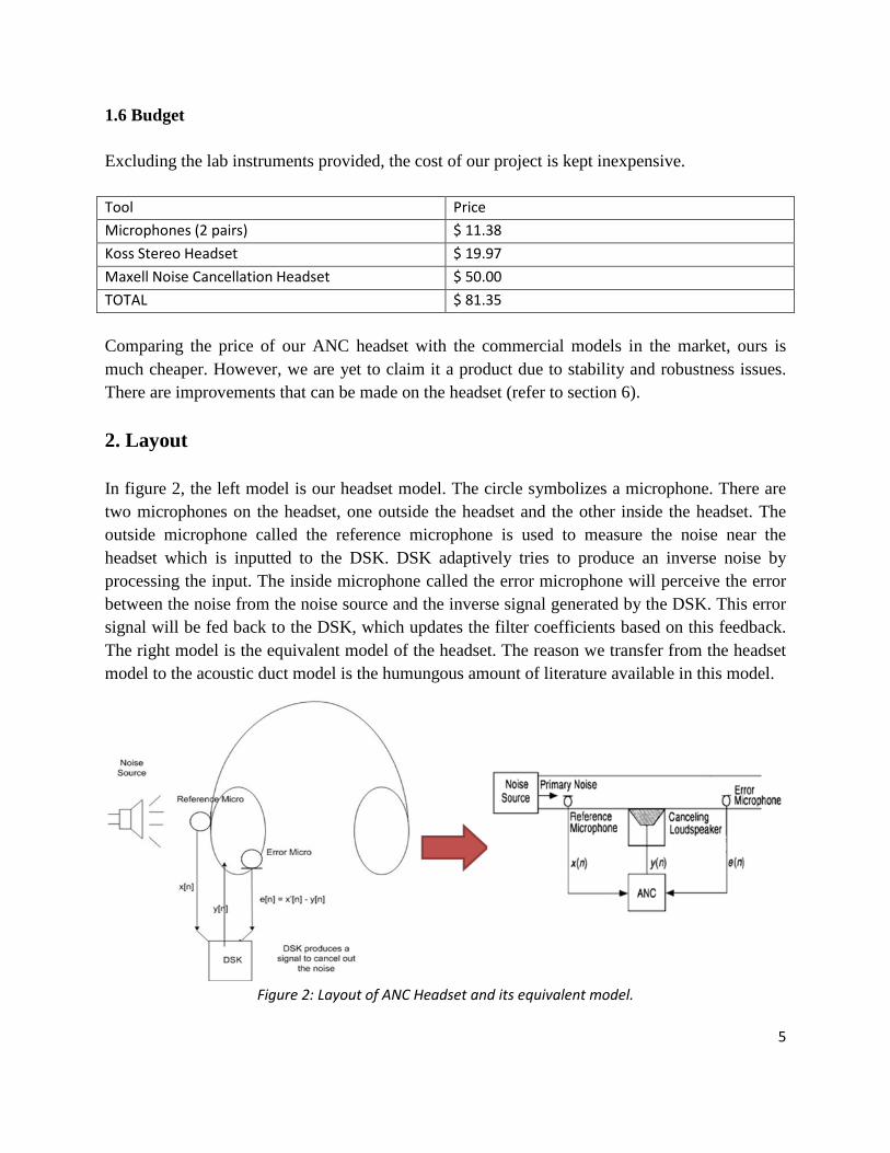
Comparing the price of our ANC headset with the commercial models in the market, ours is much cheaper. However, we are yet to claim it a product due to stability and robustness issues. There are improvements that can be made on the headset (refer to section 6). 2. Layout In figure 2, the left model is our headset model. The circle symbolizes a microphone. There are two microphones on the headset, one outside the headset and the other inside the headset. The outside microphone called the reference microphone is used to measure the noise near the headset which is inputted to the DSK. DSK adaptively tries to produce an inverse noise by processing the input. The inside microphone called the error microphone will perceive the error between the noise from the noise source and the inverse signal generated by the DSK. This error signal will be fed back to the DSK, which updates the filter coefficients based on this feedback. The right model is the equivalent model of the headset. The reason we transfer from the headset model to the acoustic duct model is the humungous amount of literature available in this model.

Figure 2: Layout of ANC Headset and its equivalent model.

6

2.1 Adaptive Filter Framework Since the characteristics of the acoustic noise source and the environment are time varying, the frequency content, amplitude, phase, and sound velocity of the undesired noise are nonstationary. An ANC system must therefore be adaptive in order to cope with these variations. Adaptive filters adjust their coefficients to minimize an error signal and can be realized as (transversal) finite impulse response (FIR), (recursive) infinite impulse response (IIR), lattice, and transform-domain filters. The most common form of adaptive filter is the transversal filter using the least mean-square (LMS) algorithm. Figure 3 shows a framework of adaptive filter. Basically, there is an adjustable filter with input X and output Y. Our goal is to minimize the difference between ‘d’ and ‘Y’, where ‘d’ is the desired signal. Once the difference is computed, the adaptive algorithm will adjust the filter coefficients with the difference. There are many adaptive algorithms available in literature, the most popular ones being LMS (least mean-square) and RLS (Recursive least squares) algorithms. In the interest of computational time, we used the LMS.

Figure 3: Adaptive Filter Framework

2.2 Challenges The left hand side of Figure 4 shows the system of ANC. The use of adaptive filter for ANC application is complicated by the fact that the summing junction represents acoustic superposition in the space from the canceling loudspeaker to the error microphone, where the primary noise is combined with the output of the adaptive filter. Hence, the model is sensitive to phase mismatch. If phase mismatch occurs, even though the inverse noise is produced, the noise you hear cannot be canceled out thoroughly. Besides, the ANC is sensitive to uncorrelated noise. If the outside micro receives the uncorrelated noise, the DSK will try to produce the inverse of the uncorrelated noise, which will degrade the performance.

We came up with three solutions to solve these difficulties. First, we have to consider the delay caused by DAC, ADC, anti-aliasing filter, and reconstruction filter. We modeled this effect with

7

another filter S(z), into the mathematical model as shown in the right plot of figure 4. Second, to reduce the delay, we use FPGA to implement DAC, ADC, and analog AAF/RF. Finally, we add some protective mechanisms to stabilize the ANC system.

Figure 4: Challenges at summing junction and solutions of system delay.

2.3 MATLAB Example Figure 5 illustrates a MATLAB simulation of noise cancellation. The first row is the original noise, the second row is the noise observed at the headset, third is the inverse noise generated by an adaptive algorithm using the DSK, and the last row is the error signal between the noise observed at the headset and the inverse noise generated by the DSK. The last plot shows that the error signal is initially very high, but as the algorithm converges, this error tends to zero thereby effectively cancelling any noise generated by the noise source.

8

0 1000 2000 3000 4000 5000 6000 7000 8000 9000 10000-50

0

50noise

0 1000 2000 3000 4000 5000 6000 7000 8000 9000 10000-20

0

20observe noise

0 1000 2000 3000 4000 5000 6000 7000 8000 9000 10000-20

0

20generate inverse waveform

0 1000 2000 3000 4000 5000 6000 7000 8000 9000 10000-20

0

20error

Figure 5: MATLAB Results

2.4 Basic outline of LMS and its variations One of the main constraints in the choice of an adaptive algorithm is its computational complexity. For the application of ANC, it is desired to choose an algorithm which is computationally very fast. Taking this into consideration, LMS algorithm became an obvious choice over RLS. The update equation for the LMS algorithm is given by

w(n+1) = w(n) + µ*e(n)*w(n)

where µ is the step size, e(n) is the error at time n and w(n) is the filter coefficients at time instant n.

To make the system more stable, we also combined two variations of LMS algorithm into our design. First, we replaced the basic LMS shown above with the leaky LMS. The update equation is now given by

w(n+1) = a*w(n) + µ*e(n)*w(n), where a <1

9

By introducing the variable ‘a’ into the updating equation, we can control the rate of change of the filter coefficients w(n), over time. Besides, we also normalize the coefficients w(n) to ensure that the output doesn’t become large. The normalizing equation is given by

w(n+1) = w(n+1) / sqrt(sum(w(n+1)))

It has been observed that the built-in function ‘sqrt’ takes a large number of cycles. Considering the computational issue in the implementation, this built in function ‘sqrt’ cannot be used to normalize the weight coefficients. Instead, we used ‘table-look-up’ method to implement the function ‘sqrt’, which is much faster.

3. Approach 1: off-line estimation of S(z)

Figure 6 illustrates the block diagram of off-line estimation of S(z). We send a sequence of training data to estimate S(z) before the setup of noise cancellation. It’s better to train the filter with white noise. But because of the limited number of coefficients of the filter, the filter will not converge to a stable state when training with white noise. Hence, we just train the filter with 200 Hz sine waveform. We tried a number of algorithms using the concept of Approach 1 which are discussed in the following subsections.

Figure 6: Block diagram of Approach 1: off-line estimation of S(z).

3.1 FxLMS Algorithm Introduction The basic LMS algorithm fails to perform well in the ANC framework. This is due to the assumption made that the output of the filter y(n) is the signal perceived at the error microphone, which is not the case in practice. The presence of the A/D, D/A converters and anti aliasing filter

10

in the path from the output of the filter to the signal received at the error microphone cause significant change in the signal y(n). This demands the need to incorporate the effect of this secondary path function S(z) in the algorithm. One solution is to place an identical filter in the reference signal path to the weight update of the LMS algorithm, which realizes the so-called filtered-X LMS (FXLMS) algorithm, see Figure 8. The FXLMS algorithm has been observed to be the most effective approach among all other solutions. Also this algorithm appears to be very tolerant to errors made in the estimation of S(z) thereby allowing offline estimation of S(z) as the most apt choice. Besides, the use of FIR filters to design W(z) makes this system very stable. But the downside is the use of high order filters that will make the algorithm run slow, and also the convergence rate of this algorithm depends on the accuracy of the estimation of S(z). The major disadvantage of this algorithm is the presence of acoustic feedback. The coupling of the acoustic wave from the canceling loudspeaker to the reference microphone will cause this acoustic feedback problem, resulting in a corrupted reference signal x(n). This can potentially lead to delayed convergence and possible non-convergence of the algorithm.

Figure 8: Block diagrams of FxLMS.

MATLAB Simulations The plots below show the error signal for the FxLMS algorithm under different filter orders and step sizes. The first plot shows that the rate of convergence of the algorithm increases with the

11

filter order. Also, the second plot depicts the increased rate of convergence with larger step sizes (The step size values µ shown in the plots are in Q15 format)

Figure 9: FxLMS - MATLAB Simulation results

12

3.2 FuLMS Algorithm Introduction The simplest approach to solving the acoustic feedback problem discussed above is to use a separate feedback cancellation, or “neutralization,” filter within the controller, which is exactly the same technique as used in acoustic echo cancellation. A duct-acoustic ANC system using the FuLMS algorithm with feedback neutralization is illustrated in Fig. 10. When feedback is present, the optimal solution of the adaptive filter is generally an IIR function with poles and zeros. The poles of an IIR filter make it possible to obtain well-matched characteristics with a lower order structure, thus requiring fewer arithmetic operations. However, the disadvantages of adaptive IIR filters are: IIR filters are not unconditionally stable; the adaptation may converge to a local minimum; and the IIR adaptive algorithms can have a relatively slow convergence rate in comparison with that of FIR filters.

Figure 10: Block diagrams of FuLMS.

MATLAB Simulations The plots below show the error signal for the FULMS algorithm under different filter orders and step sizes. It can be seen from these plots that FULMS algorithm converges faster than the

13

FxLMS algorithm, as expected. Also unlike FxLMS, here global convergence is not assured and there is no theoretical convergence proof for this algorithm. Hence the error signal is not guaranteed to decrease at each iteration. This can be seen from the first plot.

Figure 11: FuLMS – MATLAB Simulation results

14

3.3 Feedback ANC Introduction The basic idea of an adaptive feedback ANC is to estimate the primary noise and use it as a reference signal x(n). According to block diagram depicted in Figure 12, the error signal is obtained through the subtraction of primary noise, d(n), and generated inverse waveform, y(n) therefore assumed no information lost during the transition, the estimated primary noise d(n) could be regenerated by summation of error signal, e(n) and y(n). Since the reference signal comes from the estimated primary noise; therefore, the accuracy of the estimation determines the overall feedback mechanism performance. Comparing to previous algorithms, Feedback ANC has two advantages over Basic FxLMS and Filter-U LMS in reducing the quantity of microphones from a pair to signal as well as eliminating the acoustic interference between the microphones. Nevertheless, one of the most noticeable disadvantages for feedback back system is its IIR structure which produces faster convergence of LMS algorithm in tradeoff of the system stability. Moreover, since half of the information for feedback system is collected from estimation, the system is not able to catch up with aperiodical signal in terms of frequency variation.

Figure 12: Block diagrams of Feedback ANC

15

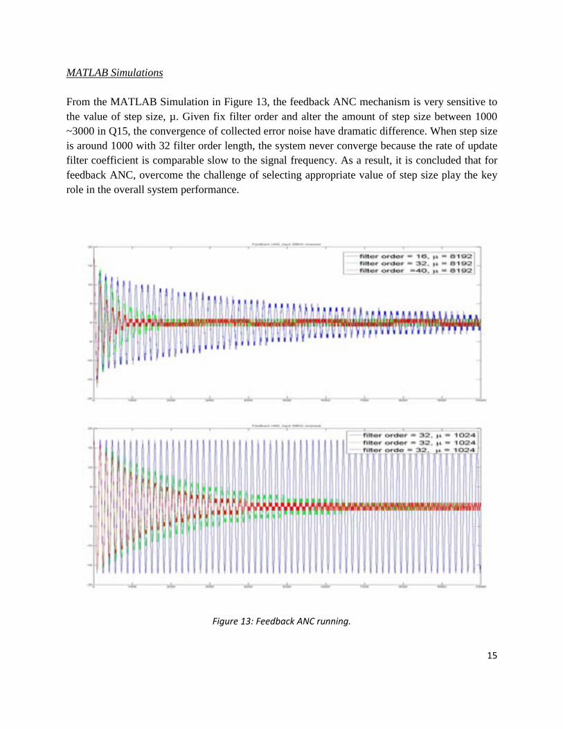
MATLAB Simulations From the MATLAB Simulation in Figure 13, the feedback ANC mechanism is very sensitive to the value of step size, µ. Given fix filter order and alter the amount of step size between 1000 ~3000 in Q15, the convergence of collected error noise have dramatic difference. When step size is around 1000 with 32 filter order length, the system never converge because the rate of update filter coefficient is comparable slow to the signal frequency. As a result, it is concluded that for feedback ANC, overcome the challenge of selecting appropriate value of step size play the key role in the overall system performance.

Figure 13: Feedback ANC running.

16

3.4 Hybrid ANC Introduction The feedforward ANC systems discussed earlier use two sensors: a reference sensor and an error sensor. The reference sensor measures the primary noise to be canceled while the error sensor monitors the performance of the ANC system. The adaptive feedback ANC system uses only an error sensor and cancels only the predictable noise components of the primary noise. A combination of the feedforward and feedback control structures is called a hybrid ANC system, as illustrated in Fig. 14. The advantages of Hybrid ANC are it combines the nice features of feedforward and feedback systems, use lower order filters and relatively more stable than feedback ANC. But it suffers a high computational complexity. Nevertheless, high computation requirements for Hybrid ANC would significant impede the real-time implementation because during one computation cycle, 8KHz in our case, the algorithm need to collect the noise information, update filter coefficients and generate inverse waveform. Moreover, in addition to standard LMS routines, overflow protection and coefficient reset would be necessary under the circumstance of large input noise. Therefore, the performance of Hybrid LMS is achieved by sacrificing the protection function of the system which should be taken into accounts during the system design.

Figure 14: Block diagrams of Hybrid ANC.

17

MATLAB Simulations The MATLAB simulation of Hybrid ANC system follows the general trend which higher filter order and larger step size would result in faster convergence rate. Nevertheless, a minor observation indicates that the Hybrid system is comparable sensitive to the length of filter order and less to the step size; however, this observation is less obvious comparing to the simulation result of Feedback ANC.

Figure 15: Hybrid ANC running.

3.5 Comparison It is interesting to compare the performance of the four algorithms in terms of convergence rate under the same criteria, which is with fixed filter length and fixed step size. In Figure 16, four LMS mechanism is compared with universal filter order 32 and step size 2000 in Q15 format.

18

From the MATLAB result, Filter-U seems to provide the best performance; however with detail inspection, Filter-U algorithm has relative high system instability in the being of noise data acquisition. Secondly, the difference between Basic and Hybrid LMS is minor but with decrement of filter order, the IIR characteristic of Hybrid LMS would have obvious advantage over the FIR-based LMS. The Feedback LMS is expected to deliver the least performance and the MATLAB simulation confirms with this assumption; nevertheless, the advantage of eliminating microphone acoustic interference is not shown during the simulation but would be significant and apparent during the real-time demonstration.,

Figure 16: Comparing the four algorithms

4. Approach 2 In approach 2, we design our own digital-to-analog and analog-to-digital interface using SPARTAN-3 FPGA board. The architecture of our system is shown in Fig. 17. The major benefit of designing our own interface is that we can use a less complicated interface with shorter delay and thus simplified the estimation problem.

19

4.1 Input/Output hardware interface. The detail circuit diagram of the input analog-to-digital interface is shown in Fig. 18, where the 7.5kHz cutoff frequency of the sallen key low pass filter is determined by experiment. The tradeoff is that with higher cutoff frequency, the delay will be shorter. And with lower cutoff frequency, the delay will be longer. The detail circuit diagram of the output digital-to-analog interface is shown in Fig. 19. The reason we let the ADC sampling rate to be 500kHz is that there will also be a constant sample delay for looping from FPGA to DSPs and back to FPGA via McBSP, so we want the data processing in ADC and FPGA working at a high clock rate.

Figure 17: Block diagram of Approach 2: System Architecture.

20

Figure 18: Input analog/digital interface

Figure 19: Output digital/analog interface

4.2 Adaptive algorithm. Upon receiving the reference signal and error signal from FPGA, the DSP uses the received data to adaptively update filter coefficient. The general block diagram of the algorithm is shown in Fig. 20. Besides the adaptive algorithm, we have also added many protection mechanisms to make the algorithm more stable. We keep track of the performance in terms of error signal and constantly backup filter coefficient of a certain period of time. If the performance of the

21

algorithm is better than the last recorded error than we let the algorithm continue to update the filter coefficient. And if not, then we reload the filter coefficient with the last backup filter coefficient. If the performance of the algorithm is bad for a long time then we also have a mechanism to reset the filter coefficient.

Figure 20: Flow Chart of Adaptive Filter

4.3 Sampling rate and filter size design constraint. Clearly the sampling rate determines the processing time constraint. And for a fixed sampling rate, the longer filter size will result in finer frequency resolution but needs longer time to update the filter coefficients and a shorter filter size sill result in coarser frequency resolution but needs less time to update. For a fixed filter size, a higher sampling rate will result in short data processing time and coarser frequency resolution but will have less artifact after DAC output (currently we did not add anti-aliasing filter after the DAC, and the DAC uses zero order hold for output analog signal). And on the opposite, under fixed filter size a lower sampling rate will result in more data processing time and finer frequency resolution but will have more artifact after the DAC output. An interesting observation is that for a fixed sampling rate even the processing time constraint is satisfied, we do not want a long filter size. The explanation is that due to the update method of the adaptive algorithm, the updating of the filter coefficient also depends on the past reference

22

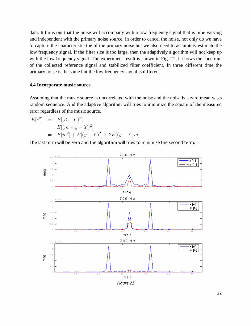
data. It turns out that the noise will accompany with a low frequency signal that is time varying and independent with the primary noise source. In order to cancel the noise, not only do we have to capture the characteristic the of the primary noise but we also need to accurately estimate the low frequency signal. If the filter size is too large, then the adaptively algorithm will not keep up with the low frequency signal. The experiment result is shown in Fig. 21. It shows the spectrum of the collected reference signal and stabilized filter coefficient. In three different time the primary noise is the same but the low frequency signal is different. 4.4 Incorporate music source. Assuming that the music source is uncorrelated with the noise and the noise is a zero mean w.s.s random sequence. And the adaptive algorithm will tries to minimize the square of the measured error regardless of the music source.

The last term will be zero and the algorithm will tries to minimize the second term.

Figure 21

23

5. Experimental Results Fig 22 to Fig 25 shows the spectrum of the noise signal and the stabilized filter coefficient.

10 20 30 40 50 600

0.5

1

1.5

2

2.5x 10

5

freq

mag

300 / 500 / 700 Hz

x[n]w[n]

Figure 22

10 20 30 40 50 600

0.5

1

1.5

2

2.5x 10

5

freq

mag

300 Hz

x[n]w[n]

Figure 23

24

10 20 30 40 50 600

0.5

1

1.5

2

2.5x 10

5

freq

mag

500 Hz

x[n]w[n]

Figure 24

10 20 30 40 50 600

0.5

1

1.5

2

2.5x 10

5

freq

mag

700 Hz

x[n]w[n]

Figure 25

25

6. Future Work Our headset has room for improvements. In the future, we will use more precise microphone and ADC, DAC to acquire more accurate measurement. We also will try to integrate the design components into a build-in embedded system to avoid feedback interference. In order to save computation cycles, we will try to implement the project in assembly language. To test our headset for stability and robustness, we will target real world noise, incorporate music source, and expand to two channels. 7. Conclusions In conclusion, we have delivered a workable ANC headset for both artificial and real world noise. More specifically, our ANC headset can deal with noise frequency ranging from 100 to 800 Hz. We have also incorporated music source. Furthermore, we have implemented and compared four variations of adaptive algorithms, namely FxLMS, FuLMS, Feedback ANC and Hybrid ANC.

8. References [1] S.M. Kuo, D.R. Morgan, Active noise control: a tutorial review, Proc. IEEE 87 (6) (June 1999) 943-975. [2] S. M. Kuo and D. R. Morgan, Active Noise Control Systems – Algorithms and DSP Implementations. New York: Wiley, 1996. [3] A. Miguez-Olivares, M. Recuero-Lopez, Development of an Active Noise Controller in the DSP Starter Kit. TI SPRA336. September 1996. [4] S. Haykin, Adaptive Filter Theory, 2nd ed. Englewood Cliffs, NJ: Prentice-Hall, 1991.

9. Appendix All the codes used for this project including C, VHDL and MATLAB are attached with the submitted zip file.