Activity 2 HYSPLIT Page 1

Activity: Using HYPSLIT to Compute Air Mass Trajectories You have just learned about the HYbrid Single-Particle Lagrangian Integrated Trajectory (HYSPLIT) transport model. HYSPLIT is provided by the U.S. National Atmospheric and Oceanic Administration (NOAA) Air Resources Laboratory (ARL). In this activity, you will practice using the on-line version of HYSPLIT to calculate air mass back trajectories. Working in a group of 2-3 participants, follow the instructions below to use HYSPLIT on your laptop computer. The instructors will be available during the activity to help answer your questions. You can use HYSPLIT to estimate the forward or backward trajectory of an air mass. Back trajectory analysis is helpful for ascertaining the origins and sources of pollutants, which makes is most useful for air quality forecasting. Forward trajectory analysis is helpful for determining the dispersion of pollutants. Note: the HYSPLIT website is in English. If you need help interpreting any part of the website, please ask one of the instructors.

1.   Go to the HYSPLIT model home page: http://ready.arl.noaa.gov/HYSPLIT_traj.php a.   For trajectories using forecasts: “Compute forecast trajectories” b.   For trajectories for past scenarios: “Compute archive trajectories”

2.   “Number of Trajectory Starting Locations”: select 1

“Type of Trajectory”: select “Normal” Click “Next”

3.   Select the “GFS Model (384h fcst, 3 hrly to 192h then 12 hrly, Global, pressure)” for forecast

and GDAS (global, 2006-present) meteorological data from the pull-down menu.

Choose a trajectory starting location using either a “Code Identifier” or “Latitude and Longitude.” The trajectory starting location should correspond to your forecast area. “Code Identifiers” are typically airport codes. Useful locations (Lat, Lon) Kuala Lumpur, Malaysia: 3.1333° N, 101.6833° E Jakarta, Indonesia: 6.1745° S, 106.8227° E Vientiane, Laos: 17.9667° N, 102.6000° E Naypyidaw, Myanmar: 19.7500° N, 96.1000° E Manila, Philippines: 14.5800° N, 121.0000° E Bangkok, Thailand: 13.7563° N, 100.5018° E Singapore: 1.3000° N, 103.8000° E

Click “Continue”

Activity 2 HYSPLIT Page 2

4.   Select the most recent “Meteorological Forecast Cycle” from the pull-down menu.

Note: the hour is in UTC time, which is Greenwich Mean Time (GMT) •   Malaysia: Local Time = GMT + 8 •   Indonesia: Local Time = GMT + 7 •   Laos: Local Time = GMT + 7 •   Myanmar: Local Time = GMT + 6.5 •   Philippines: Local Time = GMT + 8 •   Thailand: Local Time = GMT + 7 •   Singapore: Local Time = GMT + 8

5.   Select the “Default Model Parameters and Display Options”:

“Trajectory direction”: select “Backward” “Start time (UTC)”: Select the appropriate year, month, day, and hour to end your back trajectory. Typically it is useful to end your back trajectory at approximately noon on the forecast day (i.e., tomorrow). Note: the hour is in UTC time, which is Greenwich Mean Time (GMT). “Total run time (hours)”: This is the total time your trajectory will run. The default value is 24 hours, which is a good choice for a forecasting back trajectory. Depending on the conditions of your analysis, you may want to enter a different run time, such as 12 or 48 hours. “Level 1 height”: enter 500 meters AGL “Level 2 height”: enter 1000 meters AGL “Level 3 height”: enter 1500 meters AGL These are the meters above ground at which your trajectories will originate. Note: if you are running trajectories that cross mountain ranges, increase the altitudes of the start heights to account for the higher altitudes of the mountainous terrain. LEAVE EVERYTHING ELSE UNCHANGED FOR NOW Scroll to the bottom of the page and click “request trajectory”.

6.   Wait for your results (it will take a minute or two to process the trajectory). When the model

and graphics are complete, click on the link that says “GIF” near the top of the page. A new window will appear with your trajectory. To save your plot as a .gif file, right-click on the image and select “Save Picture As.” Then you can navigate to the area on your computer where you would like to save the file.

7.   Interpret your results. You should have a figure similar to the one on page 3. Answer the

following questions about your back trajectory.

Activity 2 HYSPLIT Page 3

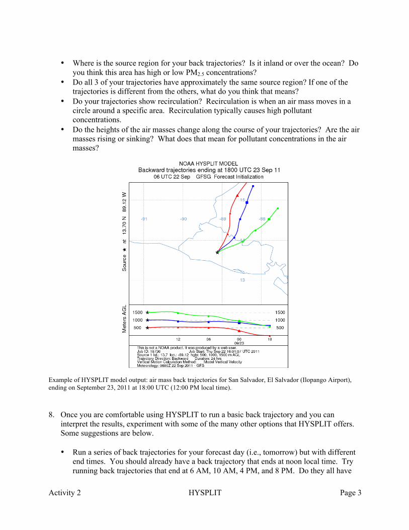
•   Where is the source region for your back trajectories? Is it inland or over the ocean? Do

you think this area has high or low PM2.5 concentrations? •   Do all 3 of your trajectories have approximately the same source region? If one of the

trajectories is different from the others, what do you think that means? •   Do your trajectories show recirculation? Recirculation is when an air mass moves in a

circle around a specific area. Recirculation typically causes high pollutant concentrations.

•   Do the heights of the air masses change along the course of your trajectories? Are the air masses rising or sinking? What does that mean for pollutant concentrations in the air masses?

Example of HYSPLIT model output: air mass back trajectories for San Salvador, El Salvador (Ilopango Airport), ending on September 23, 2011 at 18:00 UTC (12:00 PM local time). 8.   Once you are comfortable using HYSPLIT to run a basic back trajectory and you can

interpret the results, experiment with some of the many other options that HYSPLIT offers. Some suggestions are below.

•   Run a series of back trajectories for your forecast day (i.e., tomorrow) but with different

end times. You should already have a back trajectory that ends at noon local time. Try running back trajectories that end at 6 AM, 10 AM, 4 PM, and 8 PM. Do they all have

Activity 2 HYSPLIT Page 4

the same source region? Or do the origins of the back trajectories change throughout the day?

•   Change the total run time of your back trajectory from 24 hours to 12 hours or 48 hours to follow the movement of the air masses over a longer or shorter time period.

•   Change the starting heights of your back trajectory to determine the impact on the trajectory analysis. Avoid heights over approximately 2500 m (otherwise you will be above the boundary layer) or below approximately 250 m (or you will get interference from the surface).

•   Run a forward trajectory that begins at noon local time today. Forward trajectories indicate the dispersion of pollutants. Where will the air mass that is in your forecast area today be tomorrow? Will it impact your air quality forecast?

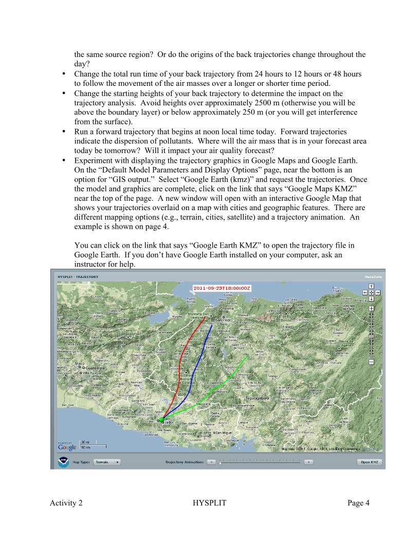
•   Experiment with displaying the trajectory graphics in Google Maps and Google Earth. On the “Default Model Parameters and Display Options” page, near the bottom is an option for “GIS output.” Select “Google Earth (kmz)” and request the trajectories. Once the model and graphics are complete, click on the link that says “Google Maps KMZ” near the top of the page. A new window will open with an interactive Google Map that shows your trajectories overlaid on a map with cities and geographic features. There are different mapping options (e.g., terrain, cities, satellite) and a trajectory animation. An example is shown on page 4. You can click on the link that says “Google Earth KMZ” to open the trajectory file in Google Earth. If you don’t have Google Earth installed on your computer, ask an instructor for help.

Activity 2 HYSPLIT Page 5

Example of HYSPLIT model output in Google Map format: air mass back trajectories for San Salvador, El Salvador (Ilopango Airport), ending on September 23, 2011 at 18:00 UTC (12:00 PM local time). Trajectory heights are 500 m (red), 1000 m (blue), and 1500 m (green). Extra Activities:

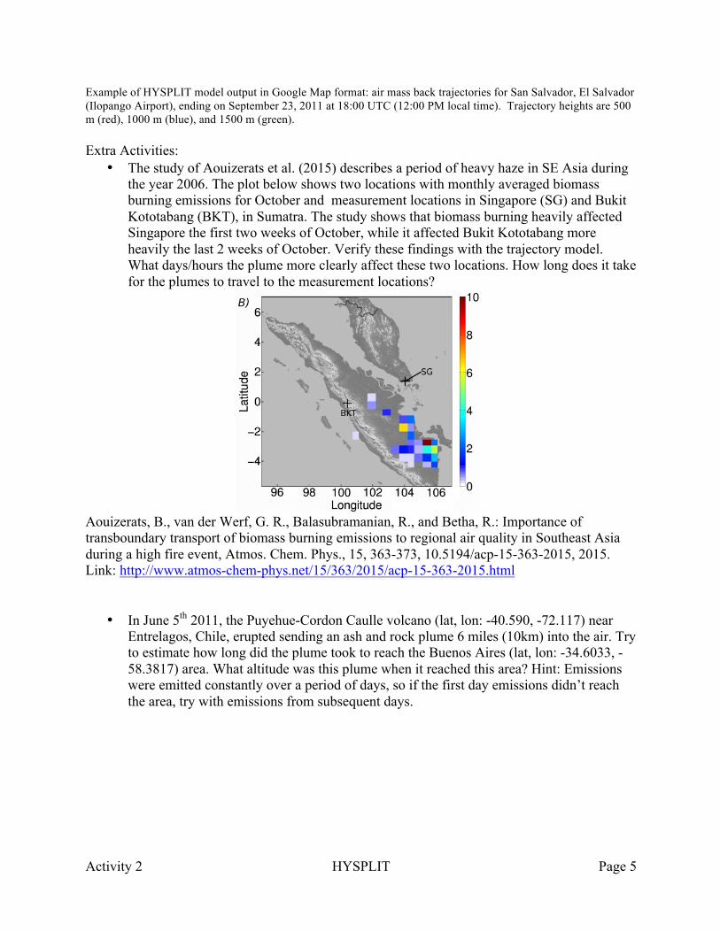
•   The study of Aouizerats et al. (2015) describes a period of heavy haze in SE Asia during the year 2006. The plot below shows two locations with monthly averaged biomass burning emissions for October and measurement locations in Singapore (SG) and Bukit Kototabang (BKT), in Sumatra. The study shows that biomass burning heavily affected Singapore the first two weeks of October, while it affected Bukit Kototabang more heavily the last 2 weeks of October. Verify these findings with the trajectory model. What days/hours the plume more clearly affect these two locations. How long does it take for the plumes to travel to the measurement locations?

Aouizerats, B., van der Werf, G. R., Balasubramanian, R., and Betha, R.: Importance of transboundary transport of biomass burning emissions to regional air quality in Southeast Asia during a high fire event, Atmos. Chem. Phys., 15, 363-373, 10.5194/acp-15-363-2015, 2015. Link: http://www.atmos-chem-phys.net/15/363/2015/acp-15-363-2015.html

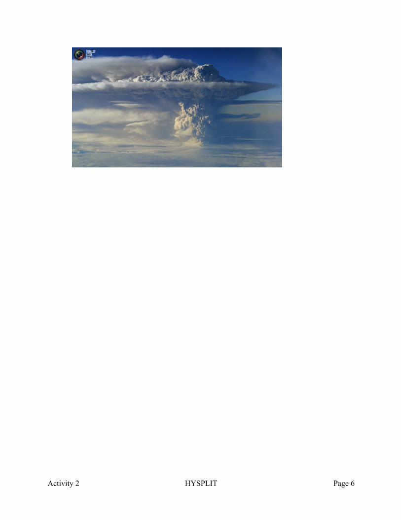
•   In June 5th 2011, the Puyehue-Cordon Caulle volcano (lat, lon: -40.590, -72.117) near Entrelagos, Chile, erupted sending an ash and rock plume 6 miles (10km) into the air. Try to estimate how long did the plume took to reach the Buenos Aires (lat, lon: -34.6033, -58.3817) area. What altitude was this plume when it reached this area? Hint: Emissions were emitted constantly over a period of days, so if the first day emissions didn’t reach the area, try with emissions from subsequent days.

Activity 2 HYSPLIT Page 6