Adapted from R. S. Sutton and A. G. Barto: Reinforcement Learning: An Introduction

From Sutton & Barto

QuickTime™ and aTIFF (Uncompressed) decompressor

are needed to see this picture.

Reinforcement LearningAn Introduction

Adapted from R. S. Sutton and A. G. Barto: Reinforcement Learning: An Introduction

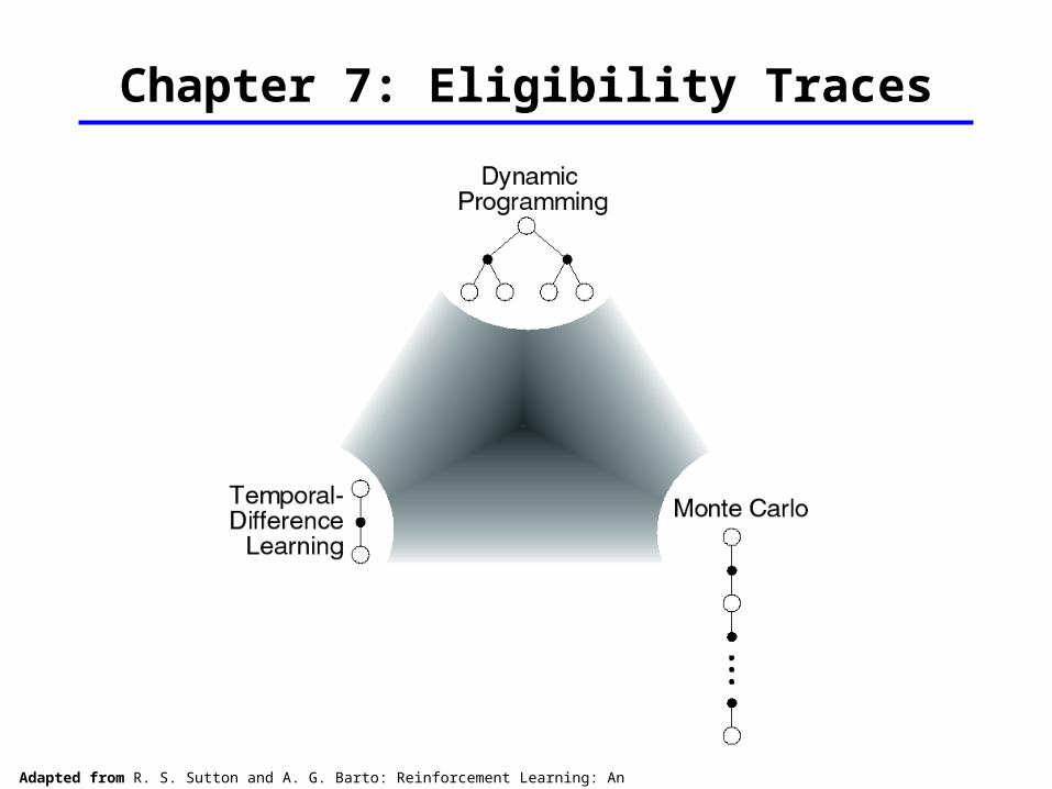
Chapter 7: Eligibility Traces

Adapted from R. S. Sutton and A. G. Barto: Reinforcement Learning: An Introduction

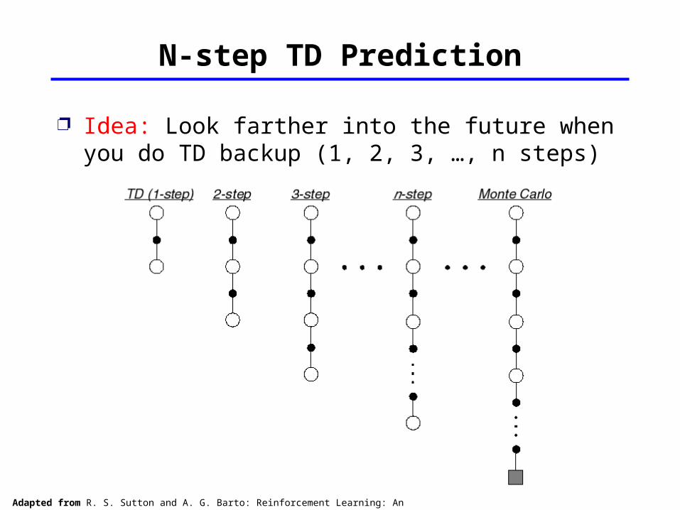
N-step TD Prediction

Idea: Look farther into the future when you do TD backup (1, 2, 3, …, n steps)

Adapted from R. S. Sutton and A. G. Barto: Reinforcement Learning: An Introduction

Monte Carlo:

TD: Use V to estimate remaining return

n-step TD: 2 step return:

n-step return:

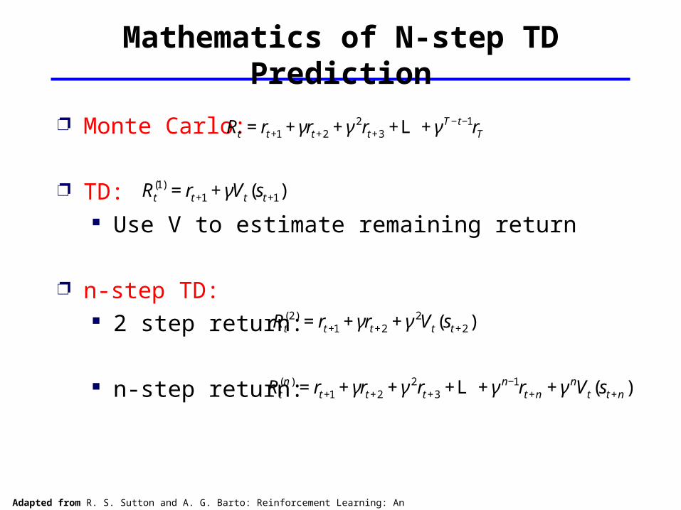
Mathematics of N-step TD Prediction

€

Rt = rt +1 + γrt +2 + γ 2rt +3 +L + γ T −t−1rT

€

Rt(1) = rt +1 + γVt (st +1)

€

Rt(2) = rt +1 + γrt +2 + γ 2Vt (st +2)

€

Rt(n ) = rt +1 + γrt +2 + γ 2rt +3 +L + γ n−1rt +n + γ nVt (st +n )

Adapted from R. S. Sutton and A. G. Barto: Reinforcement Learning: An Introduction

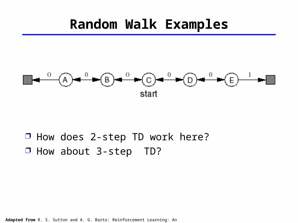
Random Walk Examples

How does 2-step TD work here? How about 3-step TD?

Adapted from R. S. Sutton and A. G. Barto: Reinforcement Learning: An Introduction

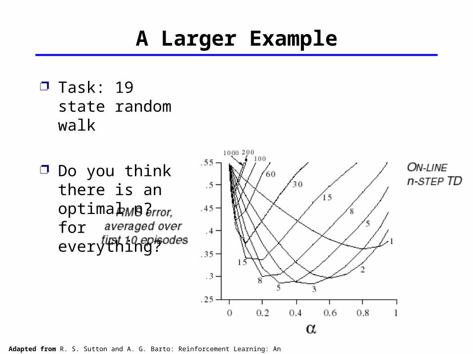
A Larger Example

Task: 19 state random walk

Do you think there is an optimal n? for everything?

Adapted from R. S. Sutton and A. G. Barto: Reinforcement Learning: An Introduction

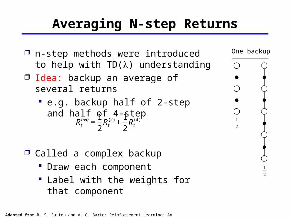
Averaging N-step Returns

n-step methods were introduced to help with TD() understanding

Idea: backup an average of several returns e.g. backup half of 2-step and half of 4-step

Called a complex backup Draw each component Label with the weights for that component

€

Rtavg =

1

2Rt

(2) +1

2Rt

(4 )

One backup

Adapted from R. S. Sutton and A. G. Barto: Reinforcement Learning: An Introduction

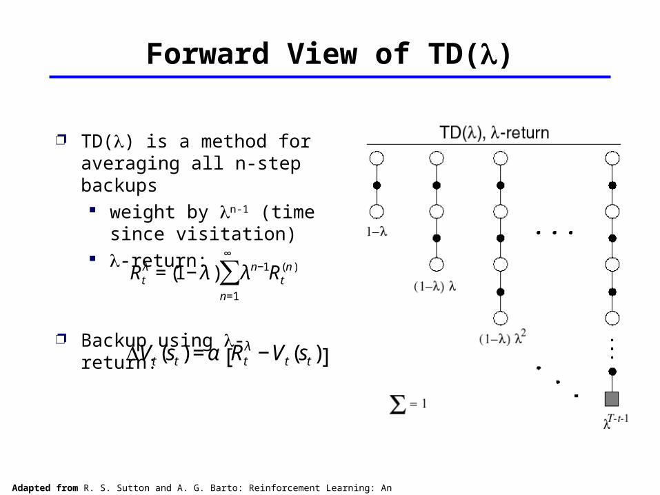
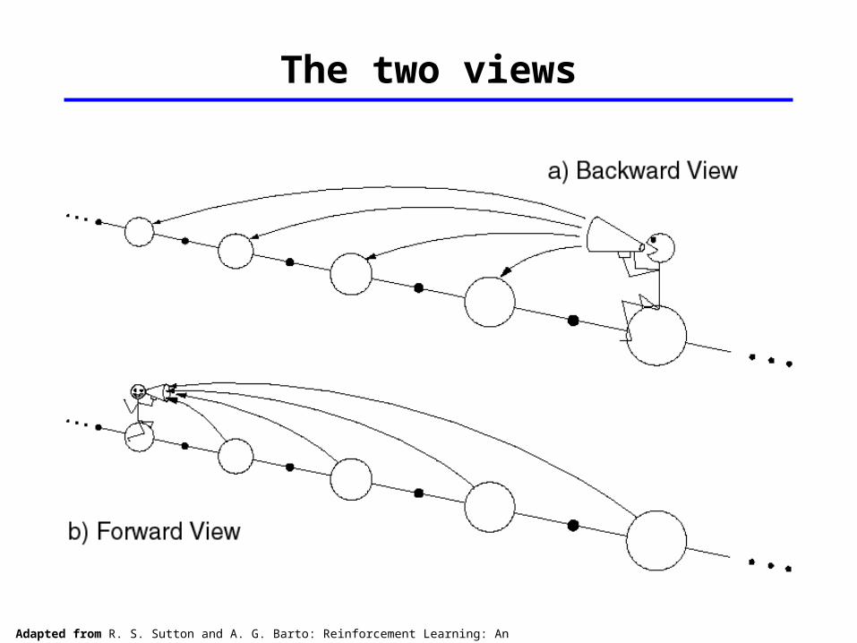
Forward View of TD()

TD() is a method for averaging all n-step backups weight by n-1 (time since visitation)

-return:

Backup using -return:€

Rtλ = (1− λ ) λn−1

n=1

∞

∑ Rt(n )

€

ΔVt (st ) = α Rtλ −Vt (st )[ ]

Adapted from R. S. Sutton and A. G. Barto: Reinforcement Learning: An Introduction

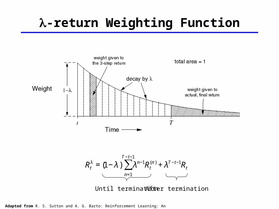
-return Weighting Function

€

Rtλ = (1− λ ) λn−1

n=1

T −t−1

∑ Rt(n ) + λT −t−1Rt

Until termination After termination

Adapted from R. S. Sutton and A. G. Barto: Reinforcement Learning: An Introduction

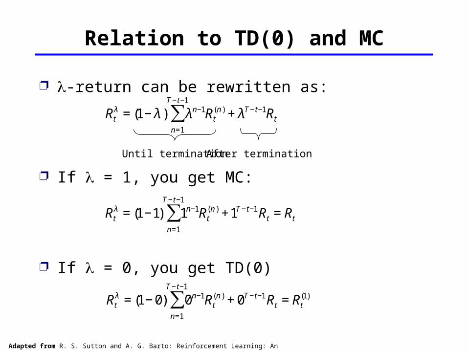
Relation to TD(0) and MC

-return can be rewritten as:

If = 1, you get MC:

If = 0, you get TD(0)

€

Rtλ = (1− λ ) λn−1

n=1

T −t−1

∑ Rt(n ) + λT −t−1Rt

€

Rtλ = (1−1) 1n−1

n=1

T −t−1

∑ Rt(n ) +1T −t−1Rt = Rt

€

Rtλ = (1− 0) 0n−1

n=1

T −t−1

∑ Rt(n ) + 0T −t−1Rt = Rt

(1)

Until termination After termination

Adapted from R. S. Sutton and A. G. Barto: Reinforcement Learning: An Introduction

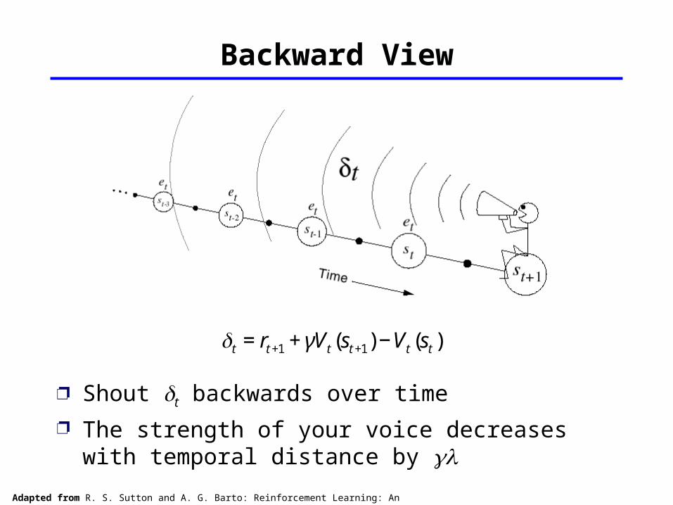
Backward View

Shout t backwards over time The strength of your voice decreases with temporal distance by

€

t = rt +1 + γVt (st +1) −Vt (st )

Adapted from R. S. Sutton and A. G. Barto: Reinforcement Learning: An Introduction

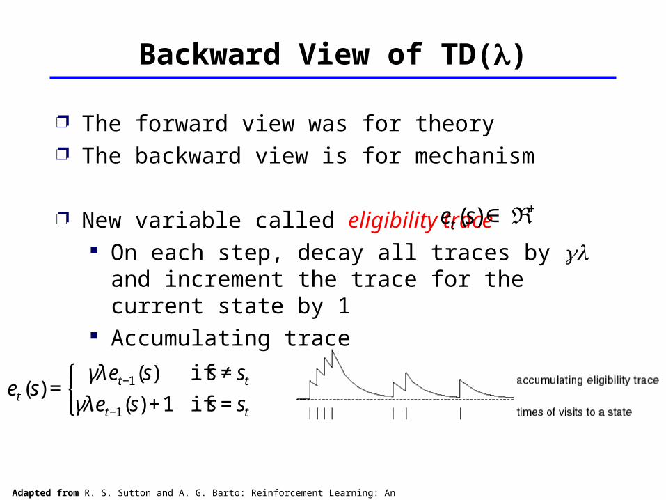
Backward View of TD()

The forward view was for theory The backward view is for mechanism

New variable called eligibility trace On each step, decay all traces by and increment the trace for the current state by 1

Accumulating trace€

et (s)∈ ℜ +

€

et (s) =γλet−1(s) if s ≠ st

γλet−1(s) +1 if s = st

⎧ ⎨ ⎩

Adapted from R. S. Sutton and A. G. Barto: Reinforcement Learning: An Introduction

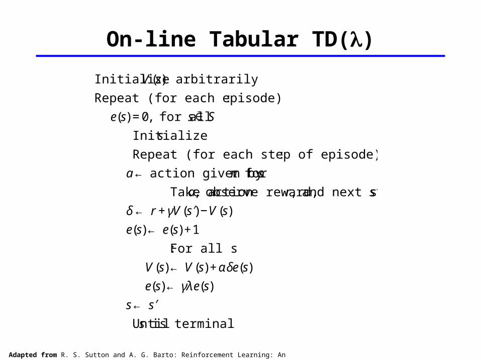
On-line Tabular TD()

€

Initialize V (s) arbitrarily

Repeat (for each episode) :

e(s) = 0, for all s∈ S

Initialize s

Repeat (for each step of episode) :

a ← action given by π for s

Take action a, observe reward, r, and next state ′ s

δ ← r + γV ( ′ s ) −V (s)

e(s) ← e(s) +1

For all s :

V (s) ← V (s) + αδe(s)

e(s) ← γλe(s)

s ← ′ s

Until s is terminal

Adapted from R. S. Sutton and A. G. Barto: Reinforcement Learning: An Introduction

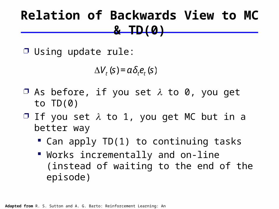
Relation of Backwards View to MC & TD(0)

Using update rule:

As before, if you set to 0, you get to TD(0)

If you set to 1, you get MC but in a better way Can apply TD(1) to continuing tasks Works incrementally and on-line (instead of waiting to the end of the episode)

€

ΔVt (s) = αδ tet (s)

Adapted from R. S. Sutton and A. G. Barto: Reinforcement Learning: An Introduction

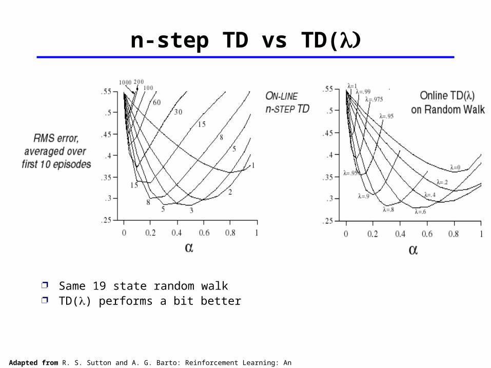
n-step TD vs TD(

Same 19 state random walk TD() performs a bit better

Adapted from R. S. Sutton and A. G. Barto: Reinforcement Learning: An Introduction

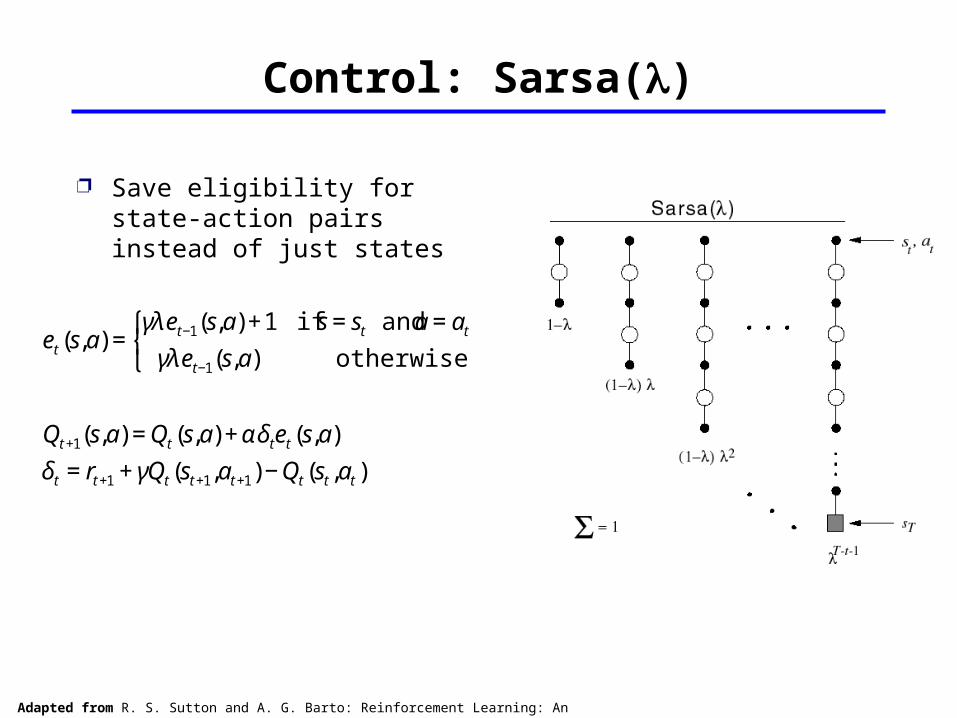
Control: Sarsa()

Save eligibility for state-action pairs instead of just states

€

et (s,a) =γλet−1(s,a) +1 if s = st and a = at

γλet−1(s,a) otherwise

⎧ ⎨ ⎩

Qt +1(s,a) = Qt (s,a) + αδ tet (s,a)

δt = rt +1 + γQt (st +1,at +1) − Qt (st ,at )

Adapted from R. S. Sutton and A. G. Barto: Reinforcement Learning: An Introduction

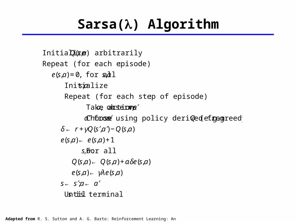
Sarsa() Algorithm

€

Initialize Q(s,a) arbitrarily

Repeat (for each episode) :

e(s,a) = 0, for all s,a

Initialize s,a

Repeat (for each step of episode) :

Take action a, observe r, ′ s

Choose ′ a from ′ s using policy derived from Q (e.g. ε - greedy)

δ ← r + γQ( ′ s , ′ a ) − Q(s,a)

e(s,a) ← e(s,a) +1

For all s,a :

Q(s,a) ← Q(s,a) + αδe(s,a)

e(s,a) ← γλe(s,a)

s ← ′ s ;a ← ′ a

Until s is terminal

Adapted from R. S. Sutton and A. G. Barto: Reinforcement Learning: An Introduction

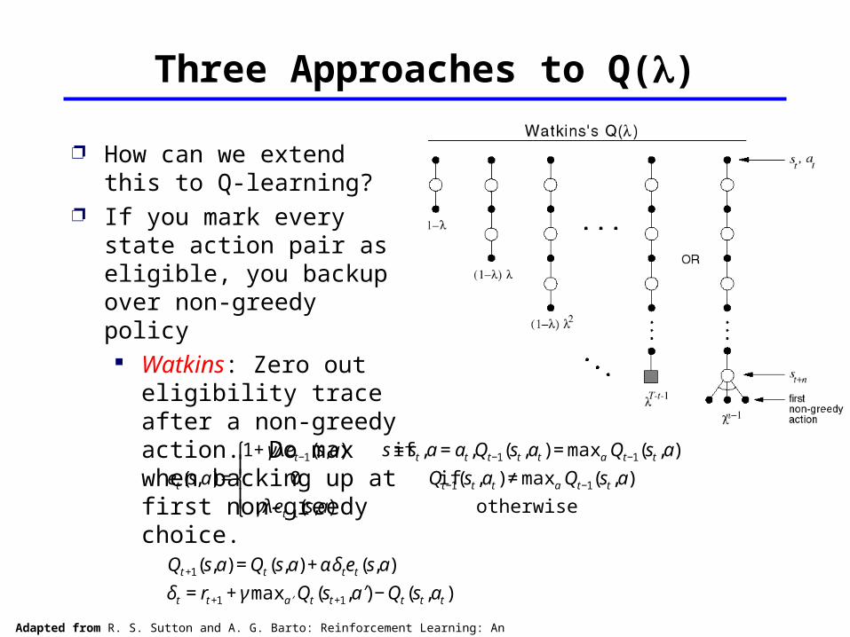
Three Approaches to Q()

How can we extend this to Q-learning?

If you mark every state action pair as eligible, you backup over non-greedy policy Watkins: Zero out eligibility trace after a non-greedy action. Do max when backing up at first non-greedy choice.

€

et (s,a) =

1+ γλet−1(s,a)

0

γλet−1(s,a)

if s = st ,a = at ,Qt−1(st ,at ) = maxa Qt−1(st ,a)

if Qt−1(st ,at ) ≠ maxa Qt−1(st ,a)

otherwise

⎧

⎨ ⎪

⎩ ⎪

Qt +1(s,a) = Qt (s,a) + αδ tet (s,a)

δt = rt +1 + γ max ′ a Qt (st +1, ′ a ) − Qt (st ,at )

Adapted from R. S. Sutton and A. G. Barto: Reinforcement Learning: An Introduction

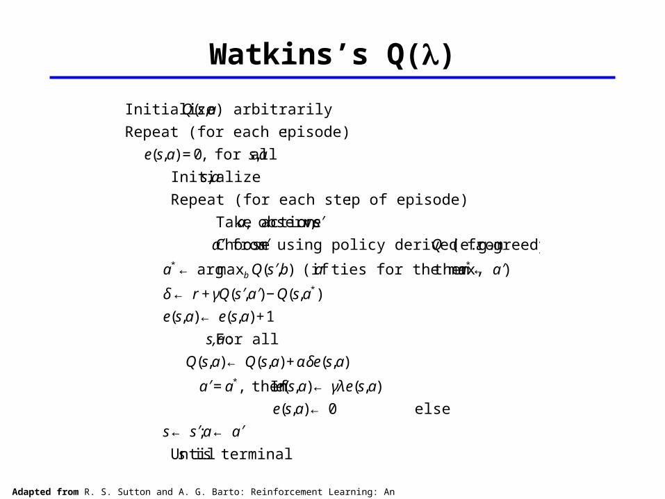
Watkins’s Q()

€

Initialize Q(s,a) arbitrarily

Repeat (for each episode) :

e(s,a) = 0, for all s,a

Initialize s,a

Repeat (for each step of episode) :

Take action a, observe r, ′ s

Choose ′ a from ′ s using policy derived from Q (e.g. ε - greedy)

a* ← argmaxb Q( ′ s ,b) (if a ties for the max, then a* ← ′ a )

δ ← r + γQ( ′ s , ′ a ) − Q(s,a*)

e(s,a) ← e(s,a) +1

For all s,a :

Q(s,a) ← Q(s,a) + αδe(s,a)

If ′ a = a*, then e(s,a) ← γλe(s,a)

else e(s,a) ← 0

s ← ′ s ;a ← ′ a

Until s is terminal

Adapted from R. S. Sutton and A. G. Barto: Reinforcement Learning: An Introduction

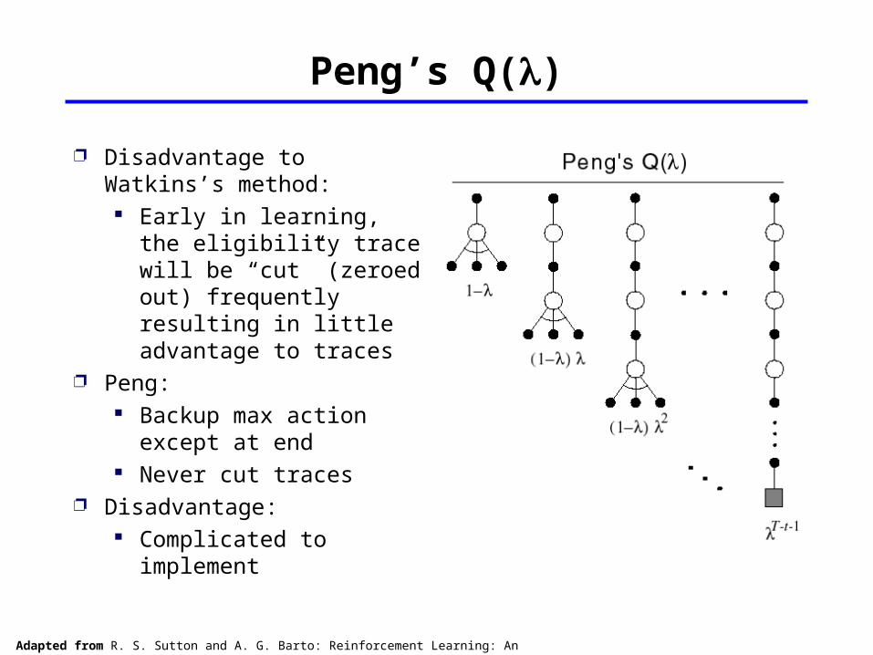
Peng’s Q()

Disadvantage to Watkins’s method: Early in learning, the eligibility trace will be “cut” (zeroed out) frequently resulting in little advantage to traces

Peng: Backup max action except at end

Never cut traces Disadvantage:

Complicated to implement

Adapted from R. S. Sutton and A. G. Barto: Reinforcement Learning: An Introduction

Naïve Q()

Idea: is it really a problem to backup exploratory actions? Never zero traces Always backup max at current action (unlike Peng or Watkins’s)

Is this truly naïve? Works well is

preliminary empirical studies

What is the backup diagram?

Adapted from R. S. Sutton and A. G. Barto: Reinforcement Learning: An Introduction

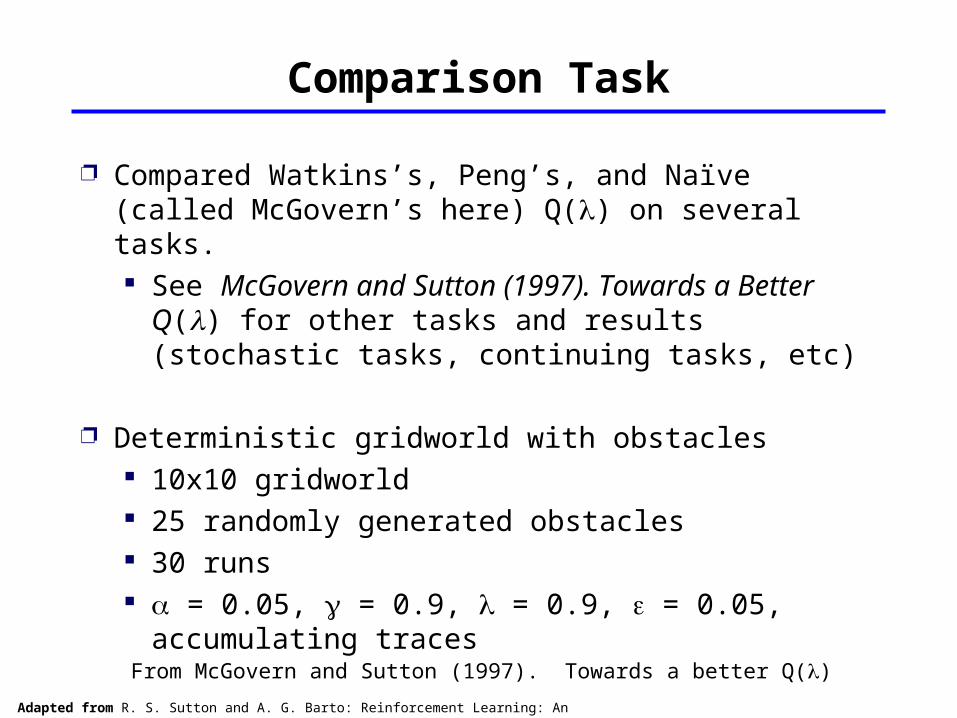
Comparison Task

From McGovern and Sutton (1997). Towards a better Q()

Compared Watkins’s, Peng’s, and Naïve (called McGovern’s here) Q() on several tasks. See McGovern and Sutton (1997). Towards a Better Q() for other tasks and results (stochastic tasks, continuing tasks, etc)

Deterministic gridworld with obstacles 10x10 gridworld 25 randomly generated obstacles 30 runs = 0.05, = 0.9, = 0.9, = 0.05, accumulating traces

Adapted from R. S. Sutton and A. G. Barto: Reinforcement Learning: An Introduction

Comparison Results

From McGovern and Sutton (1997). Towards a better Q()

Adapted from R. S. Sutton and A. G. Barto: Reinforcement Learning: An Introduction

Convergence of the Q()’s

None of the methods are proven to converge. Much extra credit if you can prove any of them.

Watkins’s is thought to converge to Q*

Peng’s is thought to converge to a mixture of Q and Q*

Naïve - Q*?

Adapted from R. S. Sutton and A. G. Barto: Reinforcement Learning: An Introduction

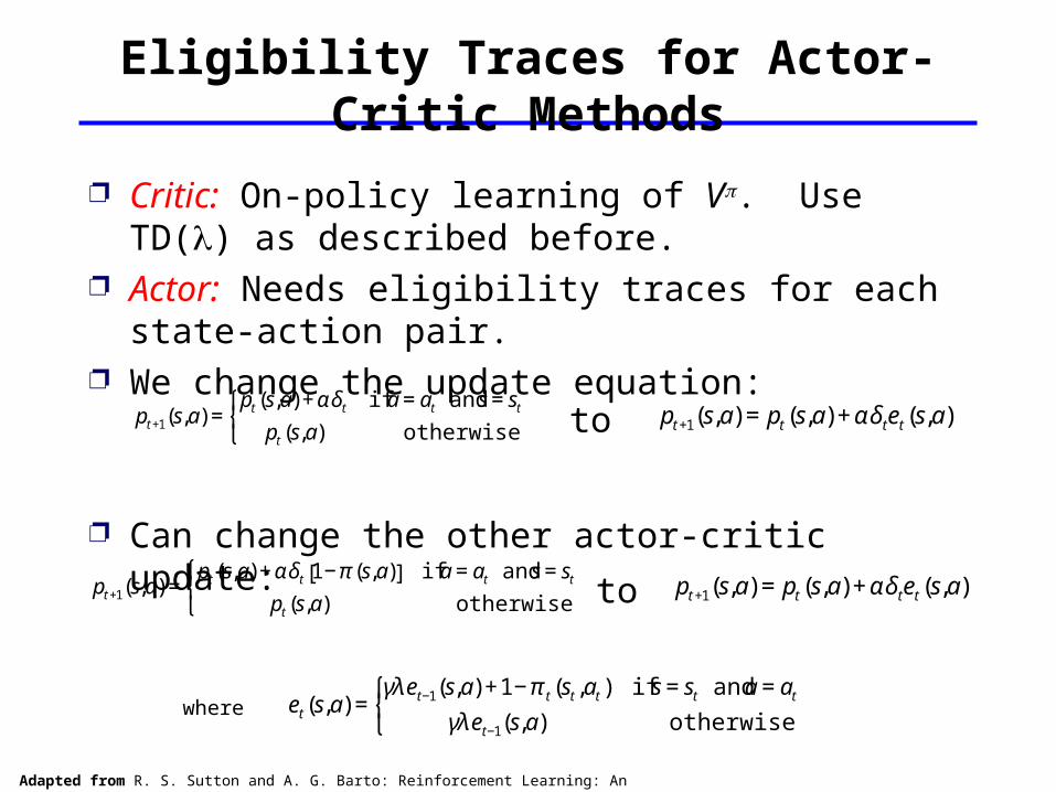
Eligibility Traces for Actor-Critic Methods

Critic: On-policy learning of V. Use TD() as described before.

Actor: Needs eligibility traces for each state-action pair.

We change the update equation:

Can change the other actor-critic update:

€

pt +1(s,a) =pt (s,a) + αδt if a = at and s = st

pt (s,a) otherwise

⎧ ⎨ ⎩

€

pt +1(s,a) = pt (s,a) + αδ tet (s,a)to

€

pt +1(s,a) =pt (s,a) + αδt 1− π (s,a)[ ] if a = at and s = st

pt (s,a) otherwise

⎧ ⎨ ⎩ to

€

pt +1(s,a) = pt (s,a) + αδ tet (s,a)

€

et (s,a) =γλet−1(s,a) +1− π t (st ,at ) if s = st and a = at

γλet−1(s,a) otherwise

⎧ ⎨ ⎩

where

Adapted from R. S. Sutton and A. G. Barto: Reinforcement Learning: An Introduction

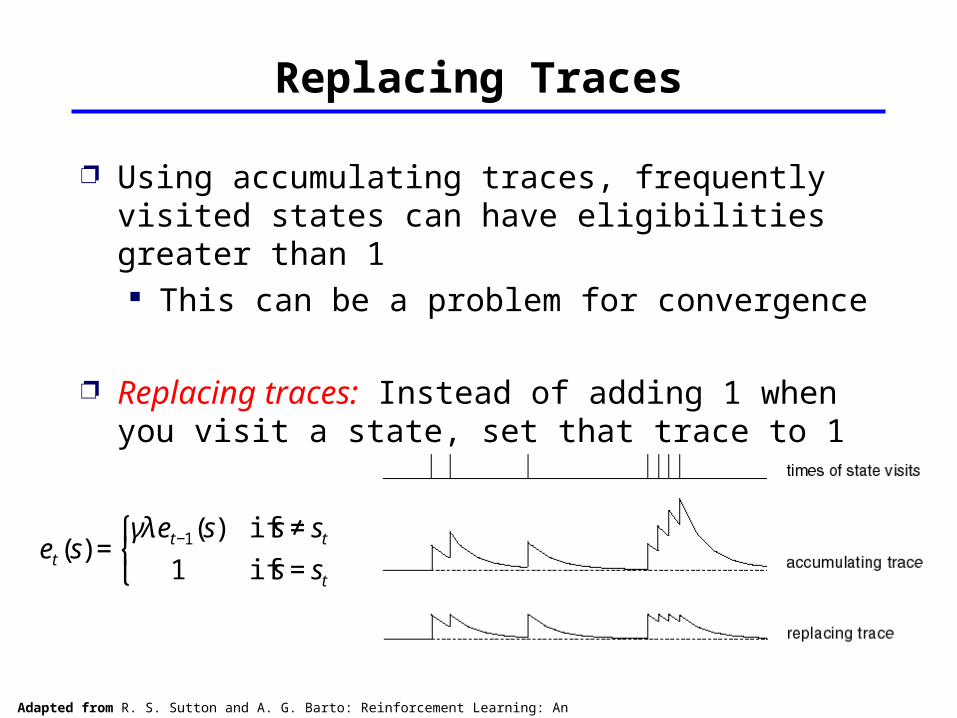
Replacing Traces

Using accumulating traces, frequently visited states can have eligibilities greater than 1 This can be a problem for convergence

Replacing traces: Instead of adding 1 when you visit a state, set that trace to 1

€

et (s) =γλet−1(s) if s ≠ st

1 if s = st

⎧ ⎨ ⎩

Adapted from R. S. Sutton and A. G. Barto: Reinforcement Learning: An Introduction

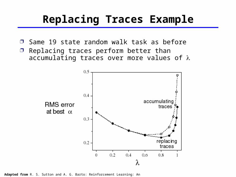
Replacing Traces Example

Same 19 state random walk task as before Replacing traces perform better than

accumulating traces over more values of

Adapted from R. S. Sutton and A. G. Barto: Reinforcement Learning: An Introduction

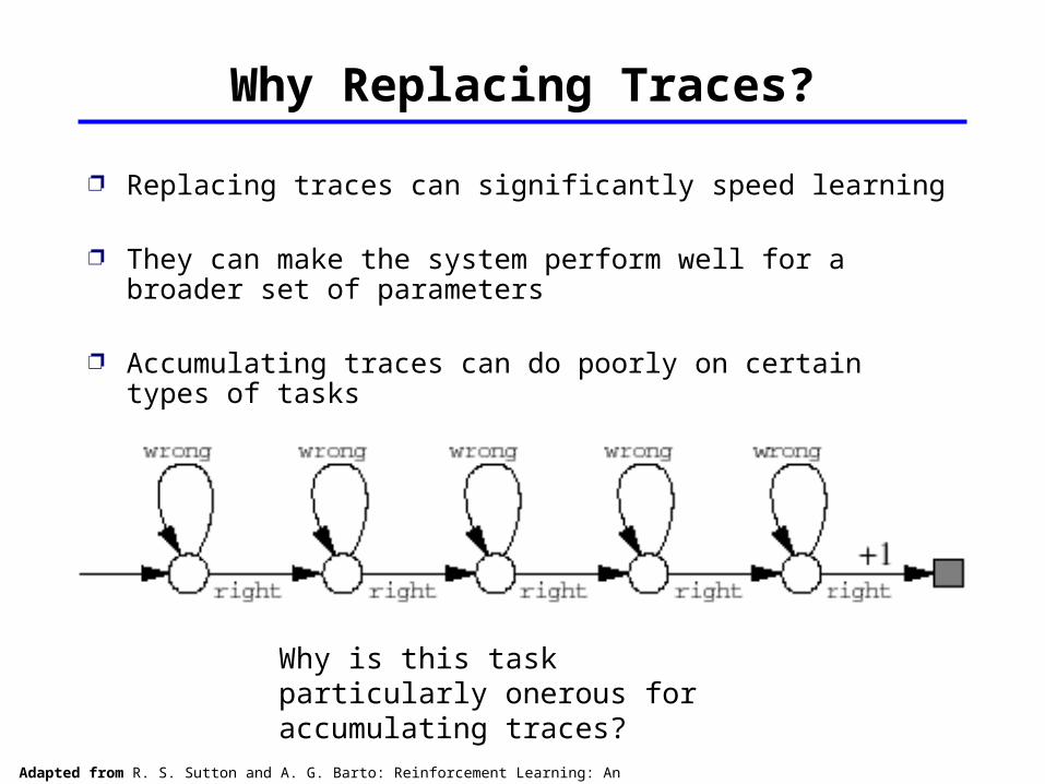
Why Replacing Traces?

Replacing traces can significantly speed learning

They can make the system perform well for a broader set of parameters

Accumulating traces can do poorly on certain types of tasks

Why is this task particularly onerous for accumulating traces?

Adapted from R. S. Sutton and A. G. Barto: Reinforcement Learning: An Introduction

More Replacing Traces

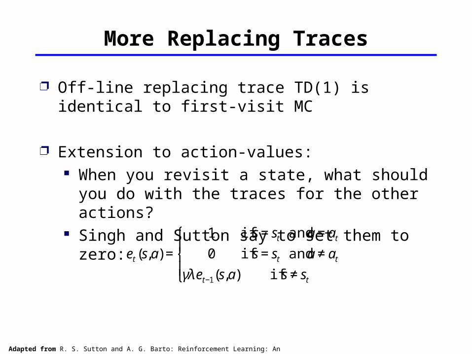
Off-line replacing trace TD(1) is identical to first-visit MC

Extension to action-values: When you revisit a state, what should you do with the traces for the other actions?

Singh and Sutton say to set them to zero:

€

et (s,a) =

1

0

γλet−1(s,a)

⎧

⎨ ⎪

⎩ ⎪

if s = st and a = at

if s = st and a ≠ at

if s ≠ st

Adapted from R. S. Sutton and A. G. Barto: Reinforcement Learning: An Introduction

Implementation Issues with Traces

Could require much more computation But most eligibility traces are VERY close to zero

If you implement it in Matlab, backup is only one line of code and is very fast (Matlab is optimized for matrices)

Adapted from R. S. Sutton and A. G. Barto: Reinforcement Learning: An Introduction

Variable

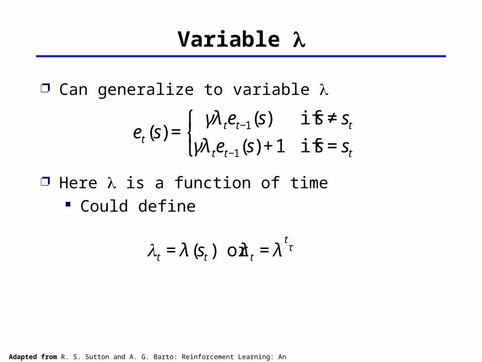
Can generalize to variable

Here is a function of time Could define €

et (s) =γλ tet−1(s) if s ≠ st

γλ tet−1(s) +1 if s = st

⎧ ⎨ ⎩

€

t = λ (st ) or λ t = λtτ

Adapted from R. S. Sutton and A. G. Barto: Reinforcement Learning: An Introduction

Conclusions

Provides efficient, incremental way to combine MC and TD Includes advantages of MC (can deal with lack of Markov property)

Includes advantages of TD (using TD error, bootstrapping)

Can significantly speed learning Does have a cost in computation

Adapted from R. S. Sutton and A. G. Barto: Reinforcement Learning: An Introduction

The two views