Adaptive defect-correction methods for viscous ... · PDF fileAdaptive defect-correction methods for viscous incompressible flow ... correction methods for viscous incompressible flow

Adaptive defect-correction methods for viscousincompressible flow problemsErvin, V.J.; Layton, W.J.; Maubach, J.M.L.

Published in:SIAM Journal on Numerical Analysis

DOI:10.1137/S0036142997318164

Published: 01/01/2000

Document VersionPublisher’s PDF, also known as Version of Record (includes final page, issue and volume numbers)

Please check the document version of this publication:

• A submitted manuscript is the author's version of the article upon submission and before peer-review. There can be important differencesbetween the submitted version and the official published version of record. People interested in the research are advised to contact theauthor for the final version of the publication, or visit the DOI to the publisher's website.• The final author version and the galley proof are versions of the publication after peer review.• The final published version features the final layout of the paper including the volume, issue and page numbers.

Link to publication

Citation for published version (APA):Ervin, V. J., Layton, W. J., & Maubach, J. M. L. (2000). Adaptive defect-correction methods for viscousincompressible flow problems. SIAM Journal on Numerical Analysis, 37(4), 1165-1185. DOI:10.1137/S0036142997318164

General rightsCopyright and moral rights for the publications made accessible in the public portal are retained by the authors and/or other copyright ownersand it is a condition of accessing publications that users recognise and abide by the legal requirements associated with these rights.

• Users may download and print one copy of any publication from the public portal for the purpose of private study or research. • You may not further distribute the material or use it for any profit-making activity or commercial gain • You may freely distribute the URL identifying the publication in the public portal ?

Take down policyIf you believe that this document breaches copyright please contact us providing details, and we will remove access to the work immediatelyand investigate your claim.

Download date: 21. May. 2018

https://doi.org/10.1137/S0036142997318164

https://research.tue.nl/en/publications/adaptive-defectcorrection-methods-for-viscous-incompressible-flow-problems(67ba5f34-cf38-4c95-97c8-6b039b8b7d73).html

ADAPTIVE DEFECT-CORRECTION METHODS FOR VISCOUSINCOMPRESSIBLE FLOW PROBLEMS∗

V. J. ERVIN† , W. J. LAYTON‡ , AND J. M. MAUBACH‡

SIAM J. NUMER. ANAL. c© 2000 Society for Industrial and Applied MathematicsVol. 37, No. 4, pp. 1165–1185

Abstract. We consider a defect correction method (DCM) which has been used extensivelyin applications where solutions have sharp transition regions, such as high Reynolds number fluidflow problems. A reliable a posteriori error estimator is derived for a defect correction method.The estimator is further studied for two examples: (a) the case of a linear-diffusion, nonlinearconvection-reaction equation, and (b) the nonlinear Navier–Stokes equations. Numerical experimentsare provided which illustrate the utility of the resulting adaptive defect correction method for highReynolds number, incompressible, viscous flow problems.

Key words. defect correction, Navier–Stokes, finite element

AMS subject classifications. Primary, 65N30; Secondary, 76M10

PII. S0036142997318164

1. Introduction. Defect-correction methods (DCMs) were originally viewed asalternates to Richardson extrapolation for increasing the formal order of finite differ-ence methods. Increasingly, however, the development of the abstract theory for theseprocedures (see, e.g., [5], [6], [10], [18], [30], [22], [23], [34], [38]) as well as the compu-tational practice of the methods (see, e.g., [17], [24], [25], [26], [27], [28]) have evolvedto using defect correction to solve much harder, nearly singular, nonlinear problemsthrough regularization and correction. This is somewhat surprising since solutions ofrepresentative applications such as high Reynolds number fluid flow problems [25],[26], [27], [28], [30], and convection-dominated, convection diffusion equations arecharacterized by sharp layers and transition regions. Thus, in spite of lacking theglobal smoothness required for the classical convergence analysis via asymptotic errorexpansions, global “uniform in epsilon” convergence in the smooth region has indeedbeen proven for defect correction methods in [5], [6], and [18] and experimentallyverified [17], [24], [25], [26], [27], [28], even for these challenging applications.

For such problems, grid refinement in sharp transition regions is necessary inconjunction with the high accuracy attained in smooth regions by defect correctiontechniques. Reliability of the resulting self-adaptive, defect-correction procedure isthen tied to the reliability of the a posteriori error estimator used for the defect-correction discretization. We consider precisely this issue herein.

Section 2 provides an a posteriori error estimator for DCMs for solving the gen-eral parameter dependent nonlinear problem F (u , ε) = 0. The estimators are ofthe residual type for an abstract realization of the defect-correction discretization.They are further developed and particularized for two representative applications:linear diffusion coupled with nonlinear convection in section 3 and the incompressibleNavier–Stokes equations (the targeted application) in section 4. Section 5 gives some

∗Received by the editors March 7, 1997; accepted for publication (in revised form) September 26,1998; published electronically March 23, 2000.

http://www.siam.org/journals/sinum/37-4/31816.html†On leave from the Department of Mathematical Sciences, Clemson University, Clemson, SC

29634 ([email protected]).‡Institute for Computational Mathematics and Applications, Department of Mathematics and

Statistics, University of Pittsburgh, Pittsburgh, PA 15260 ([email protected]). The second author waspartially supported by NSF grants DMS-9400057, DMS-9972622, INT-9814115, and INT-9805563.

1165

1166 V. J. ERVIN, W. J. LAYTON, AND J. M. MAUBACH

computational experiments with the resulting self-adaptive method.To formulate the abstract problem, method, and results, let X and Y be Banach

spaces A ∈ L(X,Y ∗), G(·) ∈ C1(X,Y ∗), and ε ∈ Λ ⊂ R Frechet differentiable. Theproblem is now to solve

F (u, ε) := A(ε)u + G(u) = 0(1.1)

for u = u(ε). The abstract DCM is given as follows. Let Xh, Yh ⊂ X,Y (respectively)be finite dimensional subspaces and Ah : Xh → Yh

∗ , Gh(·) ∈ C1(Xh, Yh∗), be (finite

dimensional) approximations of A and G(·), respectively.Let ε0 ≥ ε, Ah(ε0) be a “stabilized” or regularized approximation to Ah(ε), and let

J > 1 be given. The method studied computes u1, . . . , uJ ∈ Xh as follows: u1 ∈ Xh

satisfies

Fh(u1, ε0) := Ah(ε0)u1 + Gh(u1) = 0 ,(1.2)

whereupon successive corrections are given by, for j = 1, . . . , J ,

Ah(ε0)uj+1 + Gh(uj+1) = (Ah(ε0) −Ah(ε))uj .(1.3)

There are numerous attractive practical features of (1.2), (1.3) cited in the abovereferences. We take (1.2), (1.3) as the basic algorithm and work to find a computableupper bound for ||u−uj+1||X . To realize (1.3), the iterand uj+1 is typically computedwith a Newton method and is the root of Fε0(u) = 0 with Fε0(u) := Ah(ε0)u+Gh(u)+(Ah(ε)−Ah(ε0))uj . If the regularization is performed carefully, we often observe thatonly one or two Newton steps suffice in order to solve (1.3) for uj+1, beginning withuj , and that the resulting linearized systems are much cheaper to solve than areunregularized linear systems.

It is useful to think of (1.2) as an abstract realization of a convection-diffusionproblem in which A(ε) ∼ εA. Suppose transition regions of the underlying physicalproblems are of width ε1/α. Then a typical choice for Ah(ε0) involves increasing,on each mesh cell, ε to ε + O (mesh cell diameterα) ≈ ε + O(hαlocal), e.g., ε + O(h)for convection diffusion problems and ε + O(h2) for 2d incompressible, viscous flowproblems.

Herein we take an approach related to the local residual error estimators of [4],[7], [8], [9], [16], [19], and [43], as adapted to nonlinear problems in, e.g., [43] and [34].In contrast to most of the work on error estimators for parameterized nonlinear equa-tions, in which the goal is to construct reliably and efficiently the solution manifoldas a function of the system parameter, the goal of defect–correction-type methods isto solve a nearly singular, very large, nonlinear system (such as high Reynolds num-ber fluid flow [26], [27], [28], [29], [30]) via regularization by local effective viscosityadjustments followed by antidiffusion via correction.

2. Preliminaries. The basic assumption on (1.1) under which we proceed is thatu is a nonsingular solution of (1.1), i.e., DF (u, ε) = [A(ε) + DG(u)] ∈ Isom(X,Y ∗),and that DG(·) is Lipschitz continuous in some ball about the solution u.Theorem 2.1. Suppose that u is an isolated solution of (1.1) and that DG(u) is

Lipschitz continuous in some ball around u. Specifically, there is a R0 > 0 such that

γ := supw∈B(u;R0)

||DG(w) − DG(u)||L(X,Y ∗)

||w − u||X < ∞ .

ADAPTIVE DEFECT-CORRECTION 1167

Suppose that uj ∈ B(u;R), where

R := minR0, γ

−1||DF (u, ε)−1||−1L(Y ∗,X)

.(2.1)

Set u0 = 0 and let uj , j = 1, . . . , J , be given by (1.2), (1.3). Let Rh ∈ L(Y, Yh) be arestriction operator. Then ||u− uj+1||X is bounded as follows:

For j = 1, . . . , J − 1,

||u− uj+1||X ≤ 2||[A(ε) + DG(u)]−1||L(Y ∗,X)

||(IY − Rh)∗ [A(ε)uj+1 + G(uj+1)]||Y ∗

+ ||Rh||L(Y,Yh) ||(A(ε) −Ah(ε))uj+1 + (G−Gh)(uj+1)||Y ∗h

+ ||Rh||L(Y,Yh) ||(Ah(ε0) −Ah(ε)) (uj+1 − uj)||Y ∗h

.(2.2)

Proof. For R given by (2.1), and w ∈ B(u,R) ⊂ X,

w − u = DF (u, ε)−1

F (w, ε) +

∫ 1

0

[DF (u, ε) − DF (u + t(w − u), ε)](w − u) dt

−F (u, ε)

.

Therefore (as F (u, ε) = 0),

||w − u||X ≤ ||DF (u, ε)−1||L(Y ∗,X)

||F (w, ε) − F (u, ε)||Y ∗

+

∫ 1

0

||DF (u, ε) − DF (u + t(w − u), ε)||L(X,Y ∗)||w − u||X dt

≤ ||DF (u, ε)−1||L(Y ∗,X) ||A(ε)w + G(w)||Y ∗

+1

2||DF (u, ε)−1||L(Y ∗,X) γ ||w − u||2X .

By assumption on R, ||DF (u, ε)−1||L(Y ∗,X) γ ||w−u||X ≤ ||DF (u, ε)−1||L(Y ∗,X)γ ·R ≤ 1. Thus,

||w − u||X ≤ ||DF (u, ε)−1||L(Y ∗,X)||A(ε)w + G(w)||Y ∗ +1

2||w − u||X

and therefore,

||w − u||X ≤ 2||DF (u, ε)−1||L(Y ∗,X) ||A(ε)w + G(w)||Y ∗

≤ 2||DF (u, ε)−1||L(Y ∗,X) ||F (w, ε)||Y ∗ .

The next step is to let w := uj+1 and to use its determining equations (1.2), (1.3).To this end, consider

||F (uj+1, ε)||Y ∗ = supφ∈Y

⟨A(ε)uj+1 + G(uj+1) , φ

⟩||φ||Y

= supφ∈Y

⟨A(ε)uj+1 + G(uj+1) , φ − Rhφ

⟩− ⟨(Ah(ε) −A(ε))uj+1 + (Gh −G)(uj+1) , Rhφ

⟩+⟨(Ah(ε0) −Ah(ε))(uj+1 − uj) , Rhφ

⟩/||φ||Y .


As, Rh ∈ L(Y, Yh), it follows immediately that

||F (uj+1, ε)||Y ∗ ≤ ||(IY −Rh)∗ (A(ε)uj+1 + G(uj+1))||Y ∗

+ ||Rh||L(Y,Yh) ||(A(ε) −Ah(ε))uj+1 + (G−Gh)(uj+1)||Y ∗h

+ ||Rh||L(Y,Yh) ||(Ah(ε0) −Ah(ε))(uj+1 − uj)||Y ∗h,

which completes the proof.Remark 2.1. The terms A(ε) − Ah(ε) and G − Gh, represent consistency error

terms and will normally be of higher order. Thus the error estimator will normallybe dominated by the residual term ||(IY − Rh)∗ (A(ε)uj+1 + G(uj+1))||Y ∗ and theupdate ||(Ah(ε0) − Ah(ε))(uj+1 − uj)||Y ∗

h. One example in which consistency error

terms can be significant is when Gh includes terms arising from a subgridscale modeladded to the basic discretization.

3. A posteriori error estimators for a linear diffusion–nonlinear con-

vection problem. Let Ω ⊂ R2, X = Y :=

o

W1,2

(Ω). Set ||u||X = ||∇u||L2(Ω) anddefine F (u, ε) via the Riesz representation theorem as the element of X∗ satisfying

〈F (u, ε) , φ〉 :=

∫Ω

[ε∇u · ∇φ + g(∇u, u)φ − fφ] dx .(3.1)

Then, u is a solution of F (u, ε) = 0 in X if and only if u is a weak solution of theconvection-diffusion-reaction equation: −εu + g(∇u, u) = f in Ω ⊂ R

2 ,u = 0 on ∂Ω .

Let Xh = Yh ⊂ X be a conforming finite element space (assuming Ω is a polygonaldomain), for specificity, and suppose Xh contains C0 piecewise polynomials of degree≤ k on an edge-to-edge triangulation of Πh(Ω) of Ω. The triangulation, Πh(Ω), isassumed to have its “minimum angle” θmin(Πh(Ω)) bounded away from zero uniformlyin h; see, e.g., [45] for more details on these conditions.

The usual Galerkin finite element approximation of (3.1) is given by Fh(wh, ε) =0 ∈ X∗

h where, for all wh, φh ∈ Xh,

〈Fh(wh, ε) , φh〉 = 〈F (wh, ε) , φh〉 .The operators Ah , Gh(·) are defined analogously to F (·, ·) via the Riesz representationtheorem and the relations:

〈Ah(ε)wh , φh〉 =

∫Ω

ε∇wh · ∇φh dx ,

〈Ah(ε0)wh , φh〉 =∑

T∈Πh(Ω)

∫T

(ε + diam(T ))∇wh · ∇φh dx ,

〈Gh(wh) , φh〉 =

∫Ω

[g(∇wh, wh)φh − fφh] dx .

With these choices of Fh, Ah, and Gh, (1.2), (1.3) becomes the usual finite element,defect-correction discretization of (3.1).


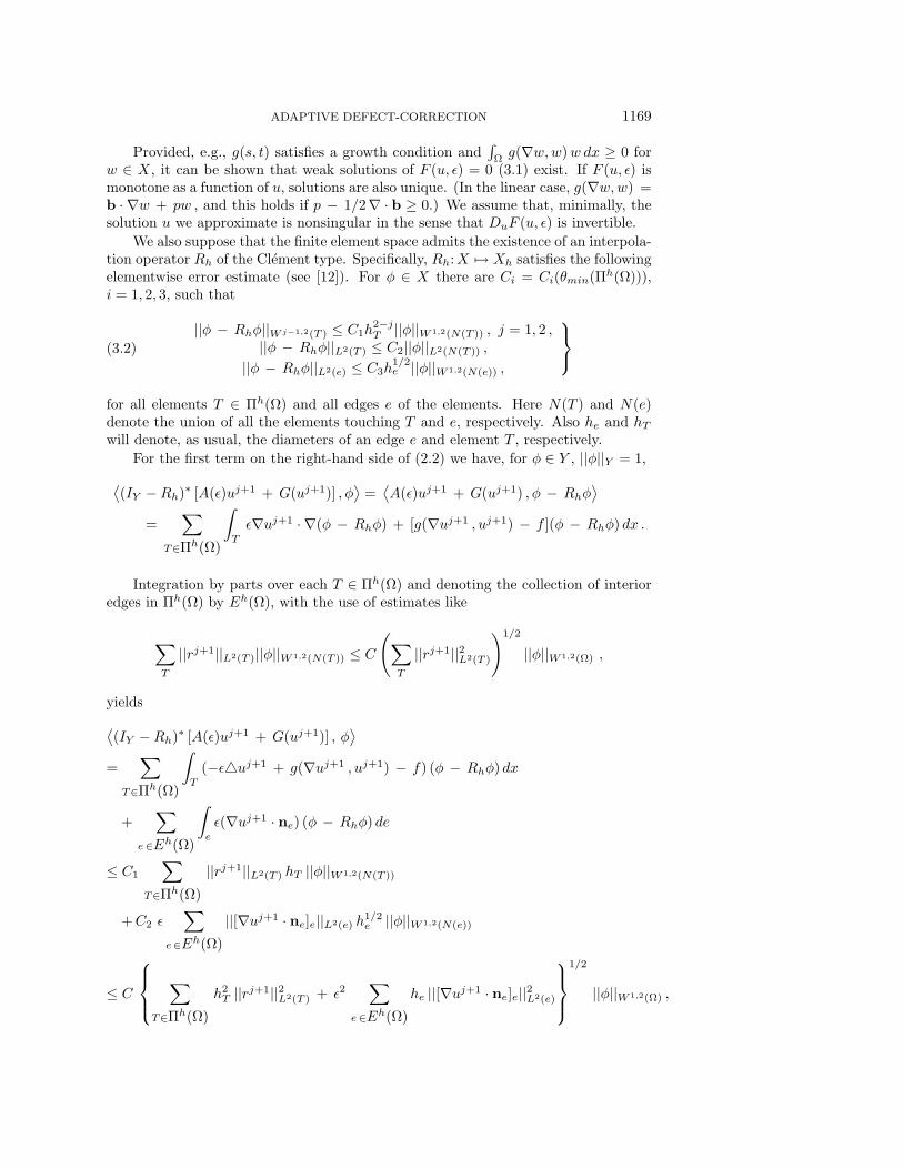
Provided, e.g., g(s, t) satisfies a growth condition and∫Ωg(∇w,w)w dx ≥ 0 for

w ∈ X, it can be shown that weak solutions of F (u, ε) = 0 (3.1) exist. If F (u, ε) ismonotone as a function of u, solutions are also unique. (In the linear case, g(∇w,w) =b · ∇w + pw , and this holds if p − 1/2∇ · b ≥ 0.) We assume that, minimally, thesolution u we approximate is nonsingular in the sense that DuF (u, ε) is invertible.

We also suppose that the finite element space admits the existence of an interpola-tion operator Rh of the Clement type. Specifically, Rh:X → Xh satisfies the followingelementwise error estimate (see [12]). For φ ∈ X there are Ci = Ci(θmin(Πh(Ω))),i = 1, 2, 3, such that

||φ − Rhφ||W j−1,2(T ) ≤ C1h2−jT ||φ||W 1,2(N(T )) , j = 1, 2 ,

||φ − Rhφ||L2(T ) ≤ C2||φ||L2(N(T )) ,

||φ − Rhφ||L2(e) ≤ C3h1/2e ||φ||W 1,2(N(e)) ,

(3.2)

for all elements T ∈ Πh(Ω) and all edges e of the elements. Here N(T ) and N(e)denote the union of all the elements touching T and e, respectively. Also he and hTwill denote, as usual, the diameters of an edge e and element T , respectively.

For the first term on the right-hand side of (2.2) we have, for φ ∈ Y , ||φ||Y = 1,

⟨(IY −Rh)∗ [A(ε)uj+1 + G(uj+1)] , φ

⟩=⟨A(ε)uj+1 + G(uj+1) , φ − Rhφ

⟩=

∑T∈Πh(Ω)

∫T

ε∇uj+1 · ∇(φ − Rhφ) + [g(∇uj+1 , uj+1) − f ](φ − Rhφ) dx .

Integration by parts over each T ∈ Πh(Ω) and denoting the collection of interioredges in Πh(Ω) by Eh(Ω), with the use of estimates like

∑T

||rj+1||L2(T )||φ||W 1,2(N(T )) ≤ C

(∑T

||rj+1||2L2(T )

)1/2

||φ||W 1,2(Ω) ,

yields

⟨(IY −Rh)∗ [A(ε)uj+1 + G(uj+1)] , φ

⟩=

∑T∈Πh(Ω)

∫T

(−εuj+1 + g(∇uj+1 , uj+1) − f) (φ − Rhφ) dx

+∑

e∈Eh(Ω)

∫e

ε(∇uj+1 · ne) (φ − Rhφ) de

≤ C1

∑T∈Πh(Ω)

||rj+1||L2(T ) hT ||φ||W 1,2(N(T ))

+C2 ε∑

e∈Eh(Ω)

||[∇uj+1 · ne]e||L2(e) h1/2e ||φ||W 1,2(N(e))

≤ C

∑T∈Πh(Ω)

h2T ||rj+1||2L2(T ) + ε2

∑e∈Eh(Ω)

he ||[∇uj+1 · ne]e||2L2(e)

1/2

||φ||W 1,2(Ω) ,


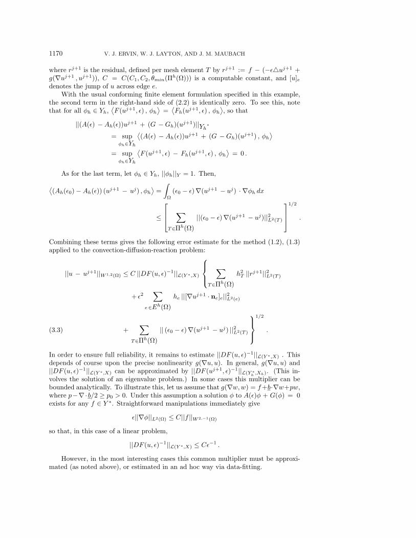
where rj+1 is the residual, defined per mesh element T by rj+1 := f − (−εuj+1 +g(∇uj+1 , uj+1)), C = C(C1, C2, θmin(Πh(Ω))) is a computable constant, and [u]edenotes the jump of u across edge e.

With the usual conforming finite element formulation specified in this example,the second term in the right-hand side of (2.2) is identically zero. To see this, notethat for all φh ∈ Yh,

⟨F (uj+1, ε) , φh

⟩=⟨Fh(uj+1, ε) , φh

⟩, so that

||(A(ε) −Ah(ε))uj+1 + (G −Gh)(uj+1)||Yh∗

= supφh∈Yh

⟨(A(ε) −Ah(ε))uj+1 + (G −Gh)(uj+1) , φh

⟩= sup

φh∈Yh

⟨F (uj+1, ε) − Fh(uj+1, ε) , φh

⟩= 0 .

As for the last term, let φh ∈ Yh, ||φh||Y = 1. Then,

⟨(Ah(ε0) −Ah(ε)) (uj+1 − uj) , φh

⟩=

∫Ω

(ε0 − ε)∇(uj+1 − uj) · ∇φh dx

≤

∑T∈Πh(Ω)

||(ε0 − ε)∇(uj+1 − uj)||2L2(T )

1/2

.

Combining these terms gives the following error estimate for the method (1.2), (1.3)applied to the convection-diffusion-reaction problem:

||u − uj+1||W 1,2(Ω) ≤ C ||DF (u, ε)−1||L(Y ∗,X)

∑T∈Πh(Ω)

h2T ||rj+1||2L2(T )

+ ε2∑

e∈Eh(Ω)

he ||[∇uj+1 · ne]e||2L2(e)

+∑

T∈Πh(Ω)

|| (ε0 − ε)∇(uj+1 − uj) ||2L2(T )

1/2

.(3.3)

In order to ensure full reliability, it remains to estimate ||DF (u, ε)−1||L(Y ∗,X) . Thisdepends of course upon the precise nonlinearity g(∇u, u). In general, g(∇u, u) and||DF (u, ε)−1||L(Y ∗,X) can be approximated by ||DF (uj+1, ε)−1||L(Y ∗

h,Xh). (This in-

volves the solution of an eigenvalue problem.) In some cases this multiplier can bebounded analytically. To illustrate this, let us assume that g(∇w,w) = f+b·∇w+pw,where p−∇·b/2 ≥ p0 > 0. Under this assumption a solution φ to A(ε)φ + G(φ) = 0exists for any f ∈ Y ∗. Straightforward manipulations immediately give

ε||∇φ||L2(Ω) ≤ C||f ||W 2,−1(Ω)

so that, in this case of a linear problem,

||DF (u, ε)−1||L(Y ∗,X) ≤ Cε−1 .

However, in the most interesting cases this common multiplier must be approxi-mated (as noted above), or estimated in an ad hoc way via data-fitting.


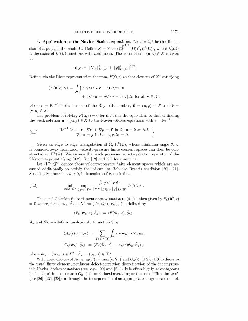
4. Application to the Navier–Stokes equations. Let d = 2, 3 be the dimen-

sion of a polygonal domain Ω. Define X = Y := ((o

W1,2

(Ω))d, L20(Ω)), where L2

0(Ω)is the space of L2(Ω) functions with zero mean. The norm of u = (u, p) ∈ X is givenby

‖u‖X := [‖∇u‖2L2(Ω) + ‖p‖2

L2(Ω)]1/2 .

Define, via the Riesz representation theorem, F (u, ε) as that element of X∗ satisfying

〈F (u, ε), v〉 =

∫Ω

[ ε ∇u : ∇v + u · ∇u · v+ q∇ · u − p∇ · v − f · v] dx for all v ∈ X ,

where ε = Re−1 is the inverse of the Reynolds number, u = (u, p) ∈ X and v =(v, q) ∈ X.

The problem of solving F (u, ε) = 0 for u ∈ X is the equivalent to that of findingthe weak solution u = (u, p) ∈ X to the Navier–Stokes equations with ε = Re−1:

−Re−1u + u · ∇u + ∇p = f in Ω, u = 0 on ∂Ω,∇ · u = g in Ω ,

∫Ωp dx = 0 .

(4.1)

Given an edge to edge triangulation of Ω, Πh(Ω), whose minimum angle θmin

is bounded away from zero, velocity-pressure finite element spaces can then be con-structed on Πh(Ω). We assume that each possesses an interpolation operator of theClement type satisfying (3.2). See [12] and [20] for examples.

Let (V h, Qh) denote those velocity-pressure finite element spaces which are as-sumed additionally to satisfy the inf-sup (or Babuska–Brezzi) condition [20], [21].Specifically, there is a β > 0, independent of h, such that

inf0 =q∈Qh

sup0 =v∈V h

∫Ωq∇ · v dx

‖∇v‖L2(Ω) ‖q‖L2(Ω)≥ β > 0 .(4.2)

The usual Galerkin-finite element approximation to (4.1) is then given by Fh(uh, ε)= 0 where, for all wh, φh ∈ Xh := (V h, Qh), Fh(·, ·) is defined by

〈Fh(wh, ε), φh〉 := 〈F (wh, ε), φh〉 .

Ah and Gh are defined analogously to section 3 by

〈Ah(ε)wh, φh〉 :=∑

T∈Πh(Ω)

∫T

ε∇wh : ∇φh dx ,

〈Gh(wh), φh〉 := 〈Fh(wh, ε) − Ah(ε)wh, φh〉 ,

where wh = (wh, q) ∈ Xh , φh := (φh, λ) ∈ Xh.With these choices of Ah, ε, ε0(T ) := maxε, hT and Gh(·), (1.2), (1.3) reduces to

the usual finite element, nonlinear defect-correction discretization of the incompress-ible Navier–Stokes equations (see, e.g., [20] and [21]). It is often highly advantageousin the algorithm to perturb Gh(·) through local averaging or the use of “flux limiters”(see [26], [27], [28]) or through the incorporation of an appropriate subgridscale model.


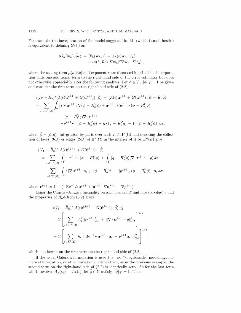
For example, the incorporation of the model suggested in [31] (which is used herein)is equivalent to defining Gh(·) as

〈Gh(wh), φh〉 := 〈Fh(wh, ε) − Ah(ε)wh , φh〉+ 〈µ(h,Re) |∇wh|r∇wh , ∇φh〉 ,

where the scaling term µ(h,Re) and exponent r are discussed in [31]. This incorpora-tion adds one additional term to the right-hand side of the error estimator but doesnot otherwise appreciably alter the following analysis. Let φ ∈ Y , ‖φ‖Y = 1 be givenand consider the first term on the right-hand side of (2.2):

〈(IY − Rh)∗[A(ε)uj+1 + G(uj+1)] , φ〉 = 〈A(ε)uj+1 + G(uj+1) , φ − Rhφ〉=

∑T∈Πh(Ω)

∫T

[ ε∇uj+1 : ∇(φ − RVh φ) + uj+1 · ∇uj+1 · (φ − RV

h φ)

+ (q − RQh q)∇ · uj+1

−pj+1∇ · (φ − RVh φ) − g · (q − RQ

h q) − f · (φ − RVh φ) ] dx,

where φ = (φ, q). Integration by parts over each T ∈ Πh(Ω) and denoting the collec-tion of faces (3-D) or edges (2-D) of Πh(Ω) in the interior of Ω by Eh(Ω) give

〈(IY − Rh)∗[A(ε)uj+1 + G(uj+1)] , φ〉=

∑T∈Πh(Ω)

∫T

−rj+1 · (φ − RVh φ) +

∫T

(q − RQh q)(∇ · uj+1 − g) dx

+∑

e∈Eh(Ω)

∫e

ε [∇uj+1 · ne]e · (φ − RVh φ) − [pj+1]e (φ − RV

h φ) · ne dσ ,

where rj+1 := f − (−Re−1uj+1 + uj+1 · ∇uj+1 + ∇pj+1).

Using the Cauchy–Schwarz inequality on each element T and face (or edge) e andthe properties of Rhφ from (3.2) gives

〈(IY − Rh)∗[A(ε)uj+1 + G(uj+1)] , φ〉 ≤

C

∑T∈Πh(Ω)

h2T ‖rj+1‖2

0,T + ||∇ · uj+1 − g‖20,T

1/2

+ C

∑e∈Eh(Ω)

he ‖[Re−1∇uj+1 · ne − pj+1ne]e‖20,e

1/2

,

which is a bound on the first term on the right-hand side of (2.2).

If the usual Galerkin formulation is used (i.e., no “subgridscale” modelling, nu-merical integration, or other variational crime) then, as in the previous example, thesecond term on the right-hand side of (2.2) is identically zero. As for the last termwhich involves Ah(ε0) − Ah(ε), let φ ∈ Y satisfy ‖φ‖Y = 1. Then,


〈(Ah(ε0) − Ah(ε) )(uj+1 − uj ) , φ〉 =

∫Ω

(ε0 − ε)∇(uj+1 − uj) : ∇φdx

≤ ∑T∈Πh(Ω)

‖(ε0(T ) − ε)∇(uj+1 − uj)‖20,T

1/2

.

Combining these terms gives an error estimator:

‖u − uj+1‖1 + ‖p − pj+1‖

≤ C ‖DF (u, ε)−1‖L(Y ∗,X)

∑T∈Πh(Ω)

h2T ‖rj+1‖2

0,T + ||∇ · uj+1 − g‖20,T

+∑

e∈Eh(Ω)


+∑

T∈Πh(Ω)

‖(ε0(T ) − ε)∇(uj+1 − uj)‖20,T

1/2

.

Remark 4.1. If the aforementioned subgridscale model from [31] is used in theresidual calculation, then an extra term appears on the right-hand side. This termtakes the form

∑T∈Πh(Ω)

||µ(hT ,Re)|∇uj |p∇uj ||2L2(T )

1/2

.

It remains, of course, to evaluate ‖DF (u, ε)−1‖L(Y ∗,X). The Navier–Stokes equations

are not monotone so an a priori bound of this term for all possible solutions is notpossible. (Singular solutions do exist and correspond to physically interesting flowsituations.) Since ‖DF (u, ε)−1‖L(Y ∗,X) is a common multiplier of the right-hand

side of (4.3), it is not required for mesh redistribution, only for the computation of areliable upperbound in order to check if a final stopping criterion is satisfied. Unfortu-nately, in general, this multiplier can only be estimated by, e.g., solving an eigenvalueproblem on a course mesh. This amounts to replacing ‖DF (u, ε)−1‖L(Y ∗,X) by

‖DF (uj+1, ε)−1‖L(XH∗,XH), where H >> h.

5. Numerical results. We give an illustration of the effectiveness of using defectcorrection methods, with a subgridscale (SGS) model, in an adaptive calculation. Toillustrate the method we solve an equilibrium, high Reynolds number flow problem(4.9) via the DCM presented in section 1. In the tests presented herein, we use eitherthe k = 1 accurate minielement (Arnold, Brezzi, and Fortin [1]) or the second orderk = 2 accurate Taylor–Hood pair [40].

The nonlinear systems arising at each step of the method, denoted F (x) =0, were linearized by a damped inexact Newton method [14], with stopping crite-rion ||F (x)||2 < 10−8. The resulting nonsymmetric linearized systems were solvedwith Sonneveld’s [37] conjugate gradient squared (CGS) (with a Vanka-like ILU(0)preconditioner [42]). The generalized minimal residual method (GMRES) of Saadand Schultz [36] or Axelsson’s generalized conjugate gradient least squares method(GCGLS) [2], [3] can also be used. However, it is our experience that they can con-sume more computational time because they explicitly orthogonalize search directions.


The storage of more search directions further limits the number of degrees of freedomwhich can be handled. The pressure was normalized by fixing its value at one pointof the domain.

The initial guess for calculations on each newly refined grid is the solution inter-polated from the previous grid. Grid to grid interpolation is easy because the gridrefinement employed (see [32]) is hierarchical with conforming basis functions. Thus,the hierarchical mesh levels automatically provide accurate initial guesses to the non-linear solver. The few nonlinear iterations (Newton steps) required reflects both thisgood initial guess and regularization of the system inherent in DCMs.

We have purposely used the most conservative options at each step because weare testing the viability of the basic DCM, rather than the many possible efficiencyimprovements. For example, the linear and nonlinear systems were solved to essen-tially machine precision (rather than truncation error of the step in question). Forthe same reason, on each new mesh, the DCM was restarted by solving an artificialviscosity approximation followed by the corrections.

For every grid, first the artificial viscosity system (1.2) was solved, with ε0 =ε + hα. Next, k (the polynomial degree of the velocity approximation) antidiffusivedefect corrections steps (1.3) follow. Thus one defect-correction iteration was used forthe minielement, and two iterations were used for the Taylor–Hood pair.

The stopping criterion used was ||r(l)||2 < 10−11, where r(l) is the lth updatedresidual. In all examples, the nodes were numbered left to right and bottom totop. As usual, the ILU(0) preconditioner performs best for lower degree polynomialvelocity approximations, when mesh refinement is limited and when nodal supportpoints are numbered regularly. In spite of this, we experienced no difficulties usinga simple ILU(0) preconditioner, because the linear systems we solved arose from aregularized artificial viscosity approximation.

The coefficients of the discrete systems were computed with quadrature rules ofdegree 2k. All quadrature rules employed use quadrature points strictly inside thereference element. In the case of k = 1, for instance, we used rule “T2: 5-1” of degree5 from Stroud [39, p. 314]. For higher polynomial degree k, quadrature formulas weretaken from Dunavant [15]. The jump integrals over the edges, were computed with astandard Gauss–Legendre formula which is exact for all polynomials of degree 2k.

All numerical experiments used the same mesh refinement technique. The coarsegrids were of the Tucker–Whitney triangular type described by Todd [41]. The grid re-finement algorithm of [32] and [33] was used to create the finer uniform and adaptivelylocally refined meshes.

The local error indicators were based on the estimator (4.3). For an element T ,we measured the local error indicators, including a possible SGS model,

Est2α(T ) = C21

[h2T ‖rj+1‖2

0,T + ||∇ · uj+1 − g‖20,T

]+ C2

2

[∑e∈T


]

+ C23

[‖(ε0(T ) − ε)∇(uj+1 − uj)‖20,T + ||µ(hT , Re)|∇uj |p∇uj ||20,T

].(5.1)

The local error indicators sum up to our global error estimate

Est2α(Ω) :=∑

T∈Πh(Ω)

Est2α(T ).(5.2)


Table 5.1Estimated and actual energy norm error ratios for the DCM.

α Estα/Est1 Errα/Err11 1.00 1.003/2 1.81 1.022 4.07 1.91

Table 5.2Estimated and actual error ratios for the DCM.

α Estα/Est1 Errα/Err11 1.00 1.003/2 1.06 0.902 1.41 1.20

The error indicator for T , Estα(T ), depends on the amount of artificial viscosityε0 − ε =: hα. Here we choose α > 0, a real number, and h = hT , the diameter oftriangle T . The usual choice for convection diffusion problems (see [5], [18], [24], and[30]) is α = 1. Since these problems have O(ε) layers for 2d flow problems we firsttested this choice for the equilibrium Navier–Stokes equations. The optimal amountof artificial diffusion hα = ε0 − ε for the DCM is explored for the Navier–Stokesequations using an example of [29].

Test problem 5.1. On the domain [0, 1]2, we used for the exact solution (u, p)

u1 = sinπx sin 2πx, u2 = x2(1 − x) sinπy, p = (1 + y(y2 − 4)) cosπx.(5.3)

The right-hand side f = f(x, y,Re) was obtained by substituting (5.3) into theNavier–Stokes equations. The velocity u satisfies the homogeneous Dirichlet boundarycondition and is smooth uniformly in the Reynolds number.

We take Re = 104, set C1 = C2 = C3 = 1, and compute Est2α(Ω) and the trueerror for the discretization using a Taylor–Hood finite element approximation. Ratherthan estimating the common multiplier ||DF−1(u, ε)||, we tabulated the ratios of theestimated errors Estα(Ω)/Est1(Ω) and the true errors Errα(Ω)/Err1(Ω). The firstcolumn of Table 5 shows the exponent α of our artificial viscosity parameter hα. Thesecond column shows the ratios Estα(Ω)/Est1(Ω) of the estimated errors, and thelast column the ratios of the true errors.

The standard choice α = 1 appears to be the best choice for globally smooth flowproblems without transition regions.

Results from additional experiments for more physically interesting flow problems,without a known exact solution (hence only calculating the first column in the table),also suggest that the optimal artificial viscosity parameter was O(h1). A similar trendwas observed if the minielement is used for the finite element discretization; see Table5.2.

For Test Problem 5.1, the estimated error was an accurate estimate of the trueerror for our choice of constants Cj . For example, with the minielement

Est21(Ω)/Err21(Ω) ≈ 0.51/0.50 ≈ 1.02.

Table 5.2 is a clear case when energy norm optimization yields a different optimalvalue of α than optimizing the “eyeball” norm. For the latter case we obtained α = 2in Test Problem 5.2. We do not have a rigorous explanation of this discrepancy.


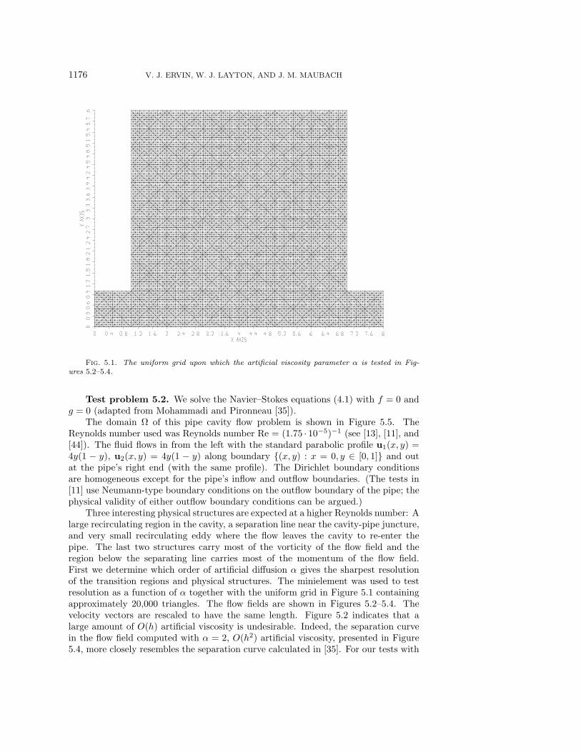
Fig. 5.1. The uniform grid upon which the artificial viscosity parameter α is tested in Fig-ures 5.2–5.4.

Test problem 5.2. We solve the Navier–Stokes equations (4.1) with f = 0 andg = 0 (adapted from Mohammadi and Pironneau [35]).

The domain Ω of this pipe cavity flow problem is shown in Figure 5.5. TheReynolds number used was Reynolds number Re = (1.75 · 10−5)−1 (see [13], [11], and[44]). The fluid flows in from the left with the standard parabolic profile u1(x, y) =4y(1 − y), u2(x, y) = 4y(1 − y) along boundary (x, y) : x = 0, y ∈ [0, 1] and outat the pipe’s right end (with the same profile). The Dirichlet boundary conditionsare homogeneous except for the pipe’s inflow and outflow boundaries. (The tests in[11] use Neumann-type boundary conditions on the outflow boundary of the pipe; thephysical validity of either outflow boundary conditions can be argued.)

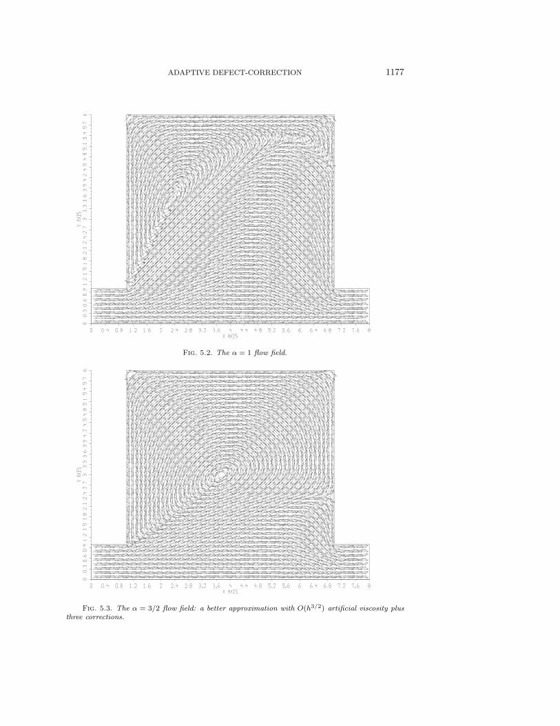
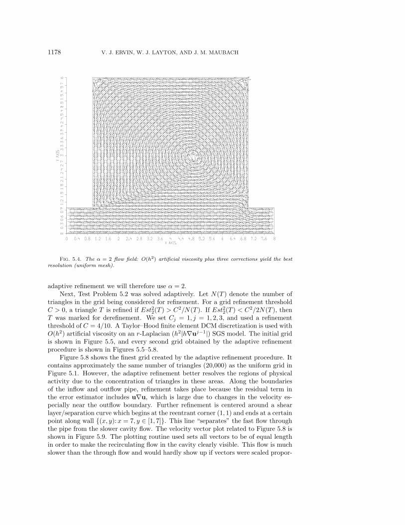
Three interesting physical structures are expected at a higher Reynolds number: Alarge recirculating region in the cavity, a separation line near the cavity-pipe juncture,and very small recirculating eddy where the flow leaves the cavity to re-enter thepipe. The last two structures carry most of the vorticity of the flow field and theregion below the separating line carries most of the momentum of the flow field.First we determine which order of artificial diffusion α gives the sharpest resolutionof the transition regions and physical structures. The minielement was used to testresolution as a function of α together with the uniform grid in Figure 5.1 containingapproximately 20,000 triangles. The flow fields are shown in Figures 5.2–5.4. Thevelocity vectors are rescaled to have the same length. Figure 5.2 indicates that alarge amount of O(h) artificial viscosity is undesirable. Indeed, the separation curvein the flow field computed with α = 2, O(h2) artificial viscosity, presented in Figure5.4, more closely resembles the separation curve calculated in [35]. For our tests with


Fig. 5.2. The α = 1 flow field.

Fig. 5.3. The α = 3/2 flow field: a better approximation with O(h3/2) artificial viscosity plusthree corrections.


Fig. 5.4. The α = 2 flow field: O(h2) artificial viscosity plus three corrections yield the bestresolution (uniform mesh).

adaptive refinement we will therefore use α = 2.Next, Test Problem 5.2 was solved adaptively. Let N(T ) denote the number of

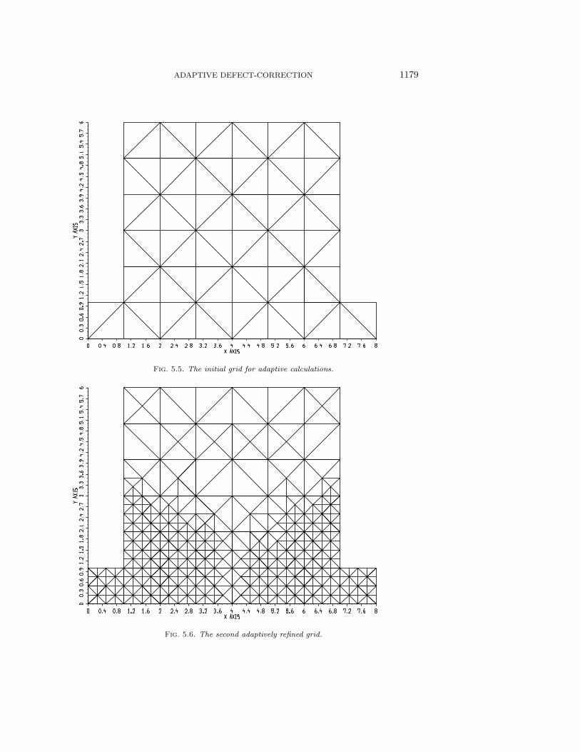
triangles in the grid being considered for refinement. For a grid refinement thresholdC > 0, a triangle T is refined if Est22(T ) > C2/N(T ). If Est22(T ) < C2/2N(T ), thenT was marked for derefinement. We set Cj = 1, j = 1, 2, 3, and used a refinementthreshold of C = 4/10. A Taylor–Hood finite element DCM discretization is used withO(h2) artificial viscosity on an r-Laplacian (h2|h∇uj−1|) SGS model. The initial gridis shown in Figure 5.5, and every second grid obtained by the adaptive refinementprocedure is shown in Figures 5.5–5.8.

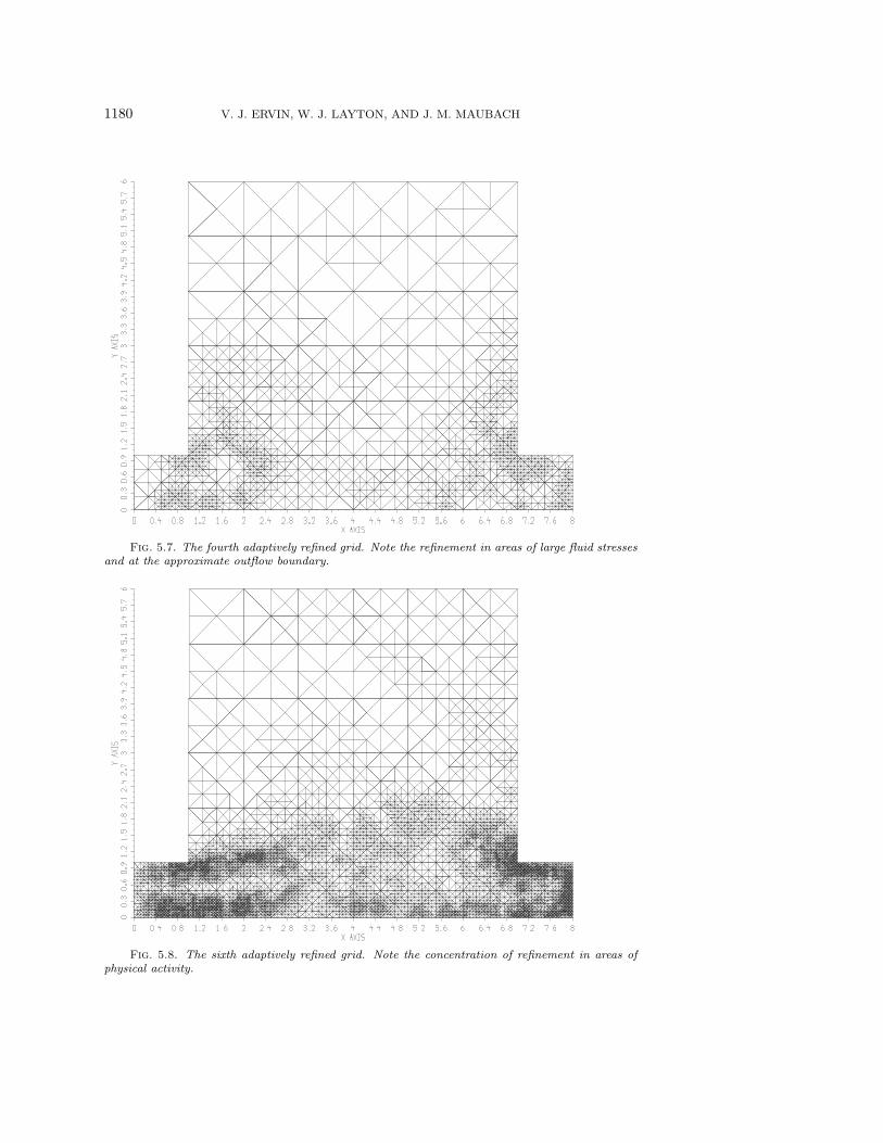
Figure 5.8 shows the finest grid created by the adaptive refinement procedure. Itcontains approximately the same number of triangles (20,000) as the uniform grid inFigure 5.1. However, the adaptive refinement better resolves the regions of physicalactivity due to the concentration of triangles in these areas. Along the boundariesof the inflow and outflow pipe, refinement takes place because the residual term inthe error estimator includes u∇u, which is large due to changes in the velocity es-pecially near the outflow boundary. Further refinement is centered around a shearlayer/separation curve which begins at the reentrant corner (1, 1) and ends at a certainpoint along wall (x, y):x = 7, y ∈ [1, 7]. This line “separates” the fast flow throughthe pipe from the slower cavity flow. The velocity vector plot related to Figure 5.8 isshown in Figure 5.9. The plotting routine used sets all vectors to be of equal lengthin order to make the recirculating flow in the cavity clearly visible. This flow is muchslower than the through flow and would hardly show up if vectors were scaled propor-


Fig. 5.5. The initial grid for adaptive calculations.

Fig. 5.6. The second adaptively refined grid.


Fig. 5.7. The fourth adaptively refined grid. Note the refinement in areas of large fluid stressesand at the approximate outflow boundary.

Fig. 5.8. The sixth adaptively refined grid. Note the concentration of refinement in areas ofphysical activity.


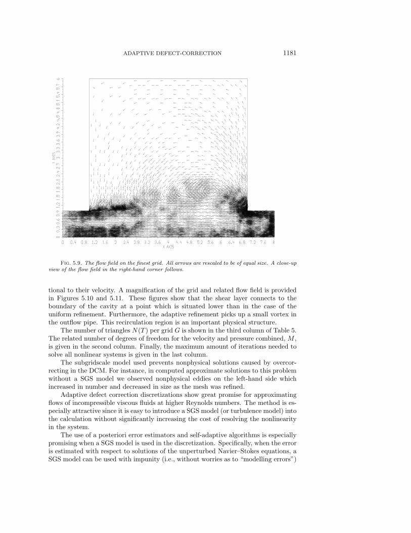
Fig. 5.9. The flow field on the finest grid. All arrows are rescaled to be of equal size. A close-upview of the flow field in the right-hand corner follows.

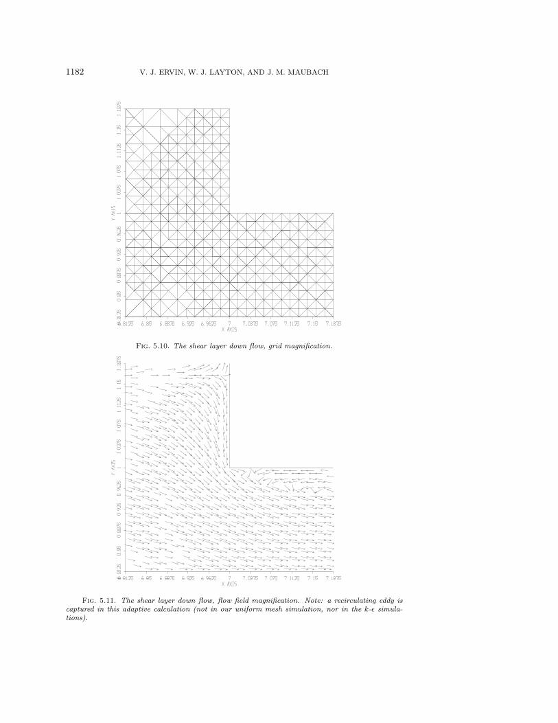
tional to their velocity. A magnification of the grid and related flow field is providedin Figures 5.10 and 5.11. These figures show that the shear layer connects to theboundary of the cavity at a point which is situated lower than in the case of theuniform refinement. Furthermore, the adaptive refinement picks up a small vortex inthe outflow pipe. This recirculation region is an important physical structure.

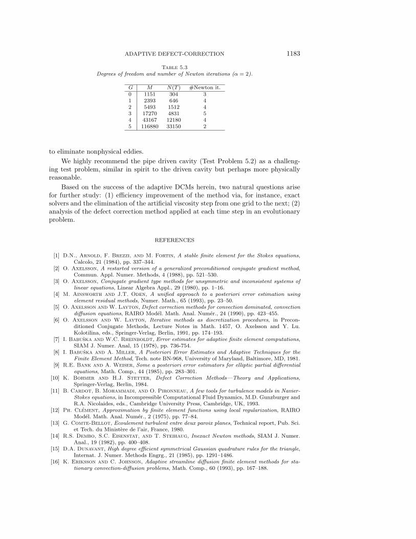
The number of triangles N(T ) per grid G is shown in the third column of Table 5.The related number of degrees of freedom for the velocity and pressure combined, M ,is given in the second column. Finally, the maximum amount of iterations needed tosolve all nonlinear systems is given in the last column.

The subgridscale model used prevents nonphysical solutions caused by overcor-recting in the DCM. For instance, in computed approximate solutions to this problemwithout a SGS model we observed nonphysical eddies on the left-hand side whichincreased in number and decreased in size as the mesh was refined.

Adaptive defect correction discretizations show great promise for approximatingflows of incompressible viscous fluids at higher Reynolds numbers. The method is es-pecially attractive since it is easy to introduce a SGS model (or turbulence model) intothe calculation without significantly increasing the cost of resolving the nonlinearityin the system.

The use of a posteriori error estimators and self-adaptive algorithms is especiallypromising when a SGS model is used in the discretization. Specifically, when the erroris estimated with respect to solutions of the unperturbed Navier–Stokes equations, aSGS model can be used with impunity (i.e., without worries as to “modelling errors”)


Fig. 5.10. The shear layer down flow, grid magnification.

Fig. 5.11. The shear layer down flow, flow field magnification. Note: a recirculating eddy iscaptured in this adaptive calculation (not in our uniform mesh simulation, nor in the k-ε simula-tions).


Table 5.3Degrees of freedom and number of Newton iterations (α = 2).

G M N(T ) #Newton it.0 1151 304 31 2393 646 42 5493 1512 43 17270 4831 54 43167 12180 45 116880 33150 2

to eliminate nonphysical eddies.

We highly recommend the pipe driven cavity (Test Problem 5.2) as a challeng-ing test problem, similar in spirit to the driven cavity but perhaps more physicallyreasonable.

Based on the success of the adaptive DCMs herein, two natural questions arisefor further study: (1) efficiency improvement of the method via, for instance, exactsolvers and the elimination of the artificial viscosity step from one grid to the next; (2)analysis of the defect correction method applied at each time step in an evolutionaryproblem.

REFERENCES

[1] D.N., Arnold, F. Brezzi, and M. Fortin, A stable finite element for the Stokes equations,Calcolo, 21 (1984), pp. 337–344.

[2] O. Axelsson, A restarted version of a generalized preconditioned conjugate gradient method,Commun. Appl. Numer. Methods, 4 (1988), pp. 521–530.

[3] O. Axelsson, Conjugate gradient type methods for unsymmetric and inconsistent systems oflinear equations, Linear Algebra Appl., 29 (1980), pp. 1–16.

[4] M. Ainsworth and J.T. Oden, A unified approach to a posteriori error estimation usingelement residual methods, Numer. Math., 65 (1993), pp. 23–50.

[5] O. Axelsson and W. Layton, Defect correction methods for convection dominated, convectiondiffusion equations, RAIRO Model. Math. Anal. Numer., 24 (1990), pp. 423–455.

[6] O. Axelsson and W. Layton, Iterative methods as discretization procedures, in Precon-ditioned Conjugate Methods, Lecture Notes in Math. 1457, O. Axelsson and Y. Lu.Kolotilina, eds., Springer-Verlag, Berlin, 1991, pp. 174–193.

[7] I. Babuska and W.C. Rheinboldt, Error estimates for adaptive finite element computations,SIAM J. Numer. Anal, 15 (1978), pp. 736-754.

[8] I. Babuska and A. Miller, A Posteriori Error Estimates and Adaptive Techniques for theFinite Element Method, Tech. note BN-968, University of Maryland, Baltimore, MD, 1981.

[9] R.E. Bank and A. Weiser, Some a posteriori error estimators for elliptic partial differentialequations, Math. Comp., 44 (1985), pp. 283–301.

[10] K. Bohmer and H.J. Stetter, Defect Correction Methods—Theory and Applications,Springer-Verlag, Berlin, 1984.

[11] B. Cardot, B. Mohammadi, and O. Pironneau, A few tools for turbulence models in Navier-Stokes equations, in Incompressible Computational Fluid Dynamics, M.D. Gunzburger andR.A. Nicolaides, eds., Cambridge University Press, Cambridge, UK, 1993.

[12] Ph. Clement, Approximation by finite element functions using local regularization, RAIROModel. Math. Anal. Numer., 2 (1975), pp. 77–84.

[13] G. Comte-Bellot, Ecoulement turbulent entre deux paroix planes, Technical report, Pub. Sci.et Tech. du Ministere de l’air, France, 1980.

[14] R.S. Dembo, S.C. Eisenstat, and T. Steihaug, Inexact Newton methods, SIAM J. Numer.Anal., 19 (1982), pp. 400–408.

[15] D.A. Dunavant, High degree efficient symmetrical Gaussian quadrature rules for the triangle,Internat. J. Numer. Methods Engrg., 21 (1985), pp. 1291–1486.

[16] K. Eriksson and C. Johnson, Adaptive streamline diffusion finite element methods for sta-tionary convection-diffusion problems, Math. Comp., 60 (1993), pp. 167–188.


[17] V. Ervin and W. Layton, High resolution, minimal storage algorithms for convection domi-nated, convection diffusion equations, in Transactions of the Fourth Army Conference onApplied Mathematics and Computing, ARO Rep., 87-1, U.S. Army Res., Triangle Park,NC, 1987, pp. 1173–1201.

[18] V. Ervin and W. Layton, A study of defect correction, finite difference methods for convectiondiffusion equations, SIAM J. Numer. Anal., 26 (1989), pp. 169–179.

[19] M.E. Cawood, V.J. Ervin, W.J. Layton, and J.M. Maubach, Adaptive defect correctionmethods for convection dominated, convection diffusion problems, J. Comput. Appl. Math.,to appear.

[20] V. Girault and P.-A. Raviart, Finite Element Methods for Navier-Stokes Equations. Theoryand Algorithms, Springer-Verlag, Berlin, 1986.

[21] M. Gunzburger, Finite Element Methods for Viscous Incompressible Flows. A Guide to The-ory, Practice and Algorithms, Academic Press, Boston, 1989.

[22] W. Hackbusch, On multigrid iterations with defect correction, in Multigrid Methods, LectureNotes in Math. 960, W. Hackbusch and V. Trottenberg, eds., Springer-Verlag, Berlin, 1982,pp. 461–473.

[23] W. Hackbusch, Multigrid Methods and Applications, Springer-Verlag, Berlin, 1985.[24] P. Hemker, Mixed defect correction iteration for the accurate solution of the convection diffu-

sion equation, in Multigrid Methods, Lecture Notes in Math. 960, W. Hackbusch and V.Trottenberg, eds., Springer-Verlag, Berlin, 1982, pp. 485–501.

[25] P. Hemker, An accurate method without directional bias for the numerical solution of a 2-Delliptic singular perturbation problem, in Theory and Applications of Singular Perturba-tions, Lecture Notes in Math. 942, W. Eckhaus and E.M. de Jaeger, eds., Springer-Verlag,Berlin, 1982, pp. 192–206.

[26] P. Hemker and B Koren, Defect correction and nonlinear multigrid for the steady Eulerequations, in Advances in Computational Fluid Dynamics, W.G. Habashi and M.M. Hafez,eds., Cambridge University Press, Cambridge, UK, 1992, pp. 273–291.

[27] P. Hemker and B. Koren, Multigrid, defect correction and upwind schemes for the steadyNavier-Stokes equations, in Numer. Methods for Fluid Dynamics III, K.W. Morton andM.J. Baines, eds, Clarendon Press, Oxford, 1988.

[28] B. Koren, Multigrid and Defect Correction for the Steady Navier-Stokes Equations, Appli-cations to Aerodynamics, C. W. I. Tract 74, Centrum voor Wiskunde en Informatica,Amsterdam, 1991.

[29] W. Layton, H.K. Lee, and J. Peterson, Numerical solution of the stationary Navier-Stokesequations using a multi-level finite element method, SIAM J. Sci. Comput., 20 (1998), pp.1–12.

[30] W. Layton, Solution algorithms for incompressible viscous flows at high Reynolds number,Vestnik Moskov Univ. Ser. XV Vychisl. Mat. Kebernet., 1 (1996), pp. 25–35.

[31] W.J. Layton, A nonlinear subgridscale model for incompressible viscous flow problems, SIAMJ. Sci. Comput., 17 (1996), pp. 347–357.

[32] J.M. Maubach, Local bisection refinement for n-simplicial grids generated by reflections, SIAMJ. Sci. Comput., 16 (1995), pp. 210–227.

[33] J. Maubach, The Amount of Similarity Classes Created by Local n-Simplicial Bisectionrefine-ment, preprint, 1996.

[34] W.C. Rheinboldt and J.L. Liu, A Posteriori Error Estimates for Parameterized NonlinearEquation, Institute for Computational Mathematics and Applications report 90-151, 1990.

[35] B. Mohammadi and O. Pironneau, Analysis of the k-ε Turbulence Model, Wiley, Chichester,UK, 1994.

[36] Y. Saad and M.H. Schultz, GMRES: A generalized minimal residual algorithm for solvingnonsymmetric linear systems, SIAM J. Sci. Statist. Comput., 7 (1986), pp. 856–869.

[37] P. Sonneveld, CGS, A fast Lanczos-type solver for nonsymmetric linear systems, SIAM J.Sci. Statist. Comput., 10 (1989), pp. 36–52.

[38] H.J. Stetter, The defect correction principle and discretization method, Numer. Math., 29(1978), pp. 425–443.

[39] A.H. Stroud, Approximate Calculation of Multiple Integrals, Prentice-Hall, New York, 1971.[40] C. Taylor and P. Hood, A numerical solution of the Navier-Stokes equations using the finite

element method, Comput. & Fluids, 1 (1973), pp. 73–100.[41] M.J. Todd, The Computation of Fixed Points and Applications, Lecture Notes in Econom.

and Math. Systems 124, Springer-Verlag, Berlin, 1976,[42] S. Vanka, Block-implit multigrid calculation of two-dimensional recirculating flows, Comput.

Methods Appl. Mech. Engrg., 59 (1986), pp. 29–48.


[43] R. Verfurth, A Review of a Posteriori Error Estimation and Adaptive Mesh RefinementTechniques, Wiley-Teubner, Chichester, UK, 1996.

[44] P.L. Viollet, On the modelling of turbulent heat and mass transfers in computations of buoy-ancy affected flows, in Proceedings of the International Conference on Numerical Methodsfor Laminar and Turbulent Flows, Venezia, 1981.

[45] O. Zienkiewicz, The Finite Element Method in Engineering Science, 3rd ed., McGraw-Hill,New York, 1977.

Documents

Adaptive defect-correction methods for viscous ... · PDF fileAdaptive defect-correction methods for viscous incompressible flow ... correction methods for viscous incompressible flow