Embed Size (px)
DESCRIPTION
Controlling meshing distortion
Citation preview
Copyright 2005 ABAQUS, Inc.
ABAQUS/Explicit: Advanced Topics
Adaptive Meshing and Distortion
Control
Lecture 6
Copyright 2005 ABAQUS, Inc.
ABAQUS/Explicit: Advanced Topics L6.2
Overview
• Introduction to Adaptive Meshing
• Lagrangian Adaptive Mesh Domains
• Eulerian Adaptive Mesh Domains for Steady-state Analyses
• Output and Diagnostics
• Additional Features of Adaptive Meshing
• Element Distortion Control
Copyright 2005 ABAQUS, Inc.
ABAQUS/Explicit: Advanced Topics
Introduction to Adaptive Meshing
Copyright 2005 ABAQUS, Inc.
ABAQUS/Explicit: Advanced Topics L6.4
Introduction to Adaptive Meshing
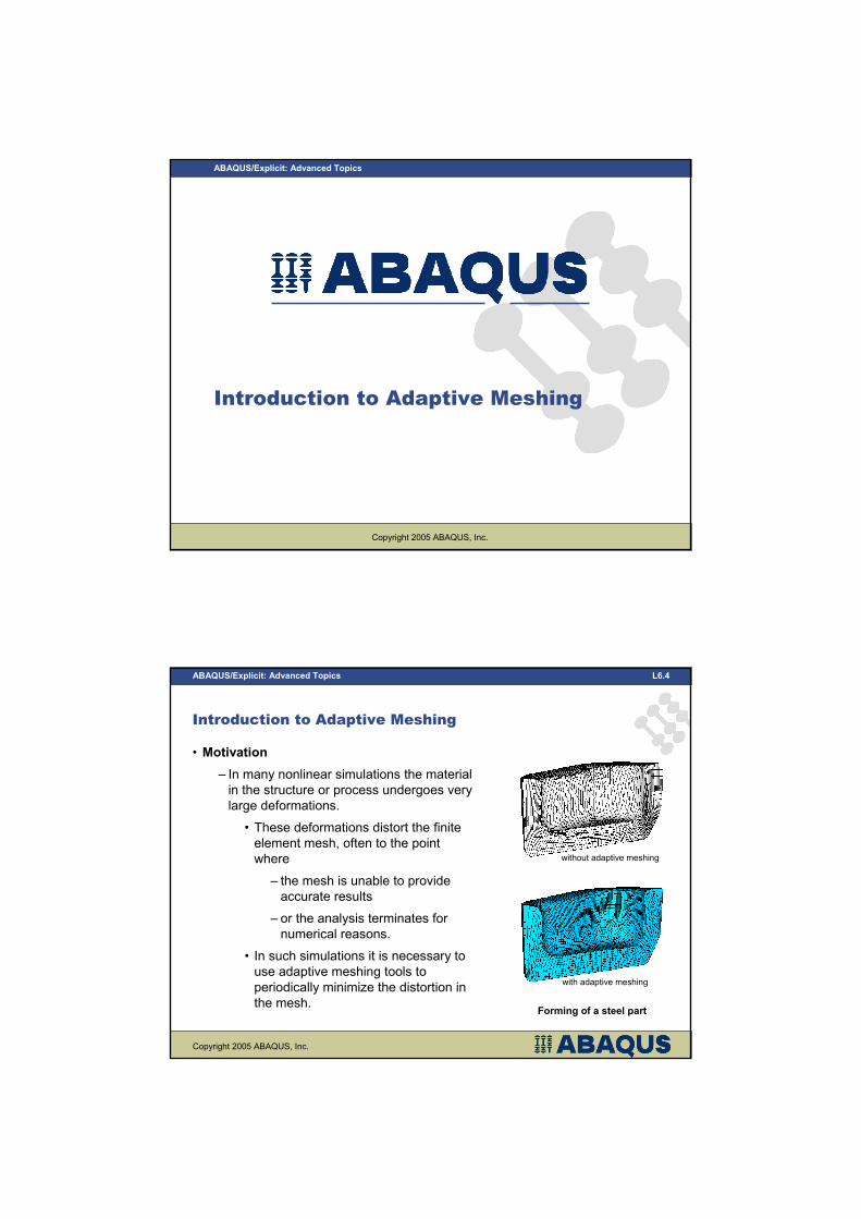
• Motivation
– In many nonlinear simulations the material
in the structure or process undergoes very
large deformations.
• These deformations distort the finite
element mesh, often to the point
where
– the mesh is unable to provide
accurate results
– or the analysis terminates for
numerical reasons.
• In such simulations it is necessary to
use adaptive meshing tools to
periodically minimize the distortion in
the mesh.
without adaptive meshing
with adaptive meshing
Forming of a steel part
Copyright 2005 ABAQUS, Inc.
ABAQUS/Explicit: Advanced Topics L6.5
Introduction to Adaptive Meshing
– ABAQUS/Explicit provides a very general and
robust adaptive meshing capability for highly
nonlinear problems ranging from quasi-static to
high-rate dynamic.
roller 1
metal
roller 2
Transient Rolling analysis
Good element
aspect ratios
minimal element
distortion
poor element
aspect ratios
severe element
distortion
with adaptive meshingwithout adaptive meshing
Video Clip
Copyright 2005 ABAQUS, Inc.
ABAQUS/Explicit: Advanced Topics L6.6
Introduction to Adaptive Meshing
• Applications
– Can be used as a continuous adaptive
meshing tool for transient analysis
problems undergoing large deformations,
such as:
• Dynamic impact
• Penetration
• Sloshing
• Forging
– Can be used as a solution technique to
model steady-state processes, such as
• Extrusion or rolling
– Can be used as a tool to analyze the
transient phase in a steady-state process
without
adaptive
meshing
with
adaptive
meshing
Impact of a copper rod
Copyright 2005 ABAQUS, Inc.
ABAQUS/Explicit: Advanced Topics L6.7
Introduction to Adaptive Meshing
• Discretization errors
– The adaptive meshing algorithm in ABAQUS/Explicit is not designed to
correct discretization errors in finite element meshes.
Copyright 2005 ABAQUS, Inc.
ABAQUS/Explicit: Advanced Topics L6.8
Introduction to Adaptive Meshing
• Pure Lagrangian description
– A pure Lagrangian model of a problem is one where the mesh moves with
the material.
• With this approach it is easy to track surfaces and to apply boundary
conditions in the problem.
• The mesh may become very distorted if the material undergoes
significant deformation;
– the quality of the results will deteriorate as the mesh becomes
distorted.
– Most problems in ABAQUS use a pure Lagrangian description.
Copyright 2005 ABAQUS, Inc.
ABAQUS/Explicit: Advanced Topics L6.9
Introduction to Adaptive Meshing
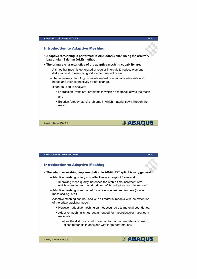
– Some simulations, such as the axisymmetric forging process shown below,
cannot be easily performed with a pure Lagrangian description.
Undeformed model
Copyright 2005 ABAQUS, Inc.
ABAQUS/Explicit: Advanced Topics L6.10
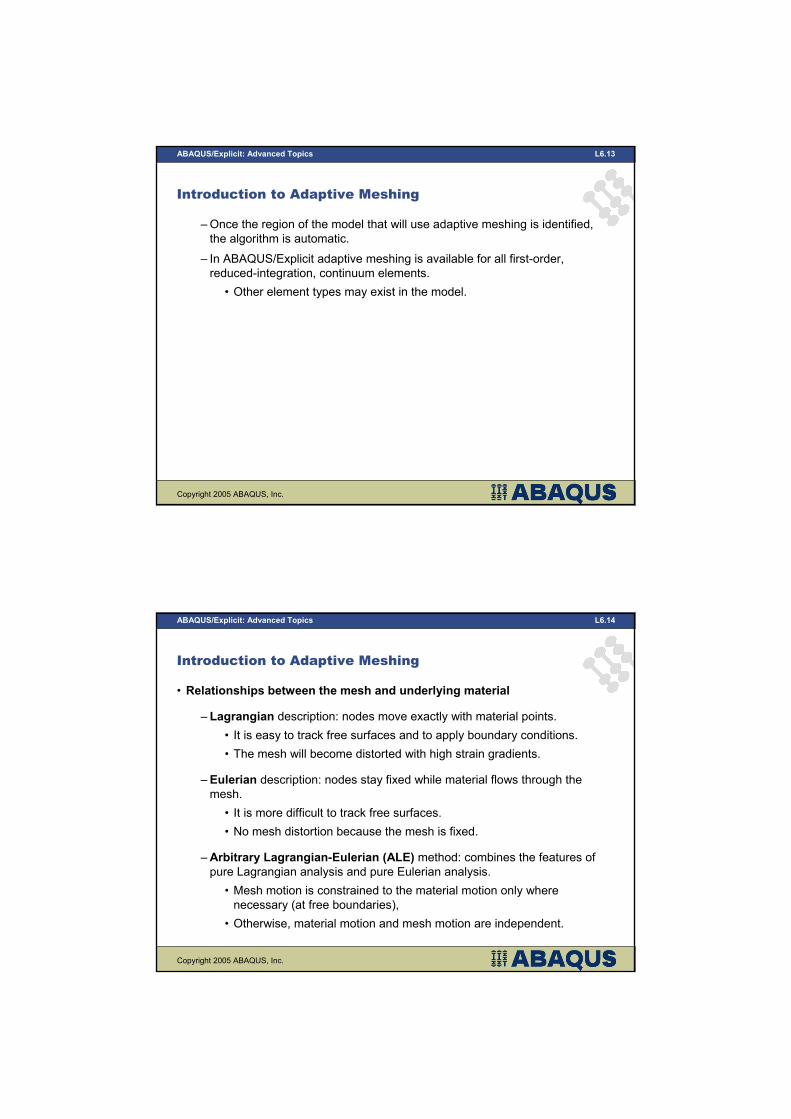
Introduction to Adaptive Meshing
– In this problem, the plastic deformation of the material creates excessive
element distortion.
– The need for adaptive meshing to reduce mesh distortion during this
analysis is clear.
70% of die travel
Lagrangian simulation deformed shape
100% of die travel
Copyright 2005 ABAQUS, Inc.
ABAQUS/Explicit: Advanced Topics L6.11
Introduction to Adaptive Meshing
• Adaptive remeshing is performed in ABAQUS/Explicit using the arbitrary
Lagrangian-Eulerian (ALE) method.
• The primary characteristics of the adaptive meshing capability are:
– A smoother mesh is generated at regular intervals to reduce element
distortion and to maintain good element aspect ratios.
– The same mesh topology is maintained—the number of elements and
nodes and their connectivity do not change.
– It can be used to analyze:
• Lagrangian (transient) problems in which no material leaves the mesh
and
• Eulerian (steady-state) problems in which material flows through the
mesh.
Copyright 2005 ABAQUS, Inc.
ABAQUS/Explicit: Advanced Topics L6.12
Introduction to Adaptive Meshing
• The adaptive meshing implementation in ABAQUS/Explicit is very general
– Adaptive meshing is very cost-effective in an explicit framework.
• Improving mesh quality increases the stable time increment size,
which makes up for the added cost of the adaptive mesh increments.
– Adaptive meshing is supported for all step-dependent features (contact,
mass scaling, etc.).
– Adaptive meshing can be used with all material models with the exception
of the brittle cracking model.
• However, adaptive meshing cannot occur across material boundaries.
• Adaptive meshing is not recommended for hyperelastic or hyperfoam
materials.
– See the distortion control section for recommendations on using
these materials in analyses with large deformations.
Copyright 2005 ABAQUS, Inc.
ABAQUS/Explicit: Advanced Topics L6.13
Introduction to Adaptive Meshing
–Once the region of the model that will use adaptive meshing is identified,
the algorithm is automatic.
– In ABAQUS/Explicit adaptive meshing is available for all first-order,
reduced-integration, continuum elements.
• Other element types may exist in the model.
Copyright 2005 ABAQUS, Inc.
ABAQUS/Explicit: Advanced Topics L6.14
Introduction to Adaptive Meshing
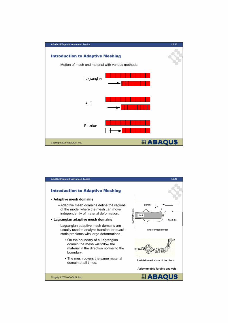
• Relationships between the mesh and underlying material
– Lagrangian description: nodes move exactly with material points.
• It is easy to track free surfaces and to apply boundary conditions.
• The mesh will become distorted with high strain gradients.
–Eulerian description: nodes stay fixed while material flows through the
mesh.
• It is more difficult to track free surfaces.
• No mesh distortion because the mesh is fixed.
–Arbitrary Lagrangian-Eulerian (ALE) method: combines the features of
pure Lagrangian analysis and pure Eulerian analysis.
• Mesh motion is constrained to the material motion only where
necessary (at free boundaries),
• Otherwise, material motion and mesh motion are independent.
Copyright 2005 ABAQUS, Inc.
ABAQUS/Explicit: Advanced Topics L6.15
Introduction to Adaptive Meshing
–Motion of mesh and material with various methods:
Copyright 2005 ABAQUS, Inc.
ABAQUS/Explicit: Advanced Topics L6.16
blank
Symmetry axis
punch
fixed die
undeformed model
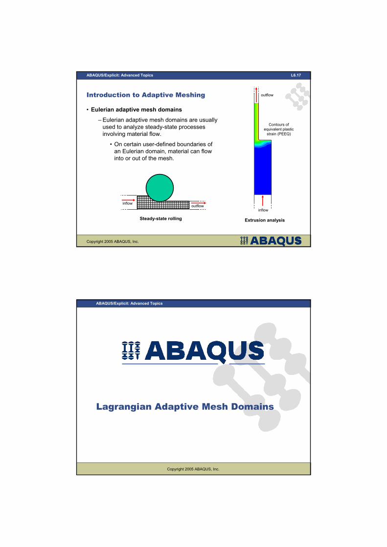
Introduction to Adaptive Meshing
• Adaptive mesh domains
– Adaptive mesh domains define the regions
of the model where the mesh can move
independently of material deformation.
• Lagrangian adaptive mesh domains
– Lagrangian adaptive mesh domains are
usually used to analyze transient or quasi-
static problems with large deformations.
• On the boundary of a Lagrangian
domain the mesh will follow the
material in the direction normal to the
boundary.
• The mesh covers the same material
domain at all times.
Axisymmetric forging analysis
final deformed shape of the blank
Copyright 2005 ABAQUS, Inc.
ABAQUS/Explicit: Advanced Topics L6.17
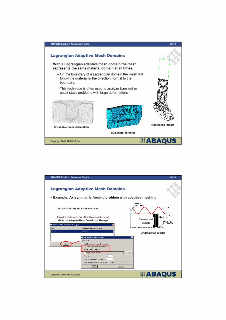
Introduction to Adaptive Meshing
• Eulerian adaptive mesh domains
– Eulerian adaptive mesh domains are usually
used to analyze steady-state processes
involving material flow.
• On certain user-defined boundaries of
an Eulerian domain, material can flow
into or out of the mesh.
Steady-state rolling
inflowoutflow
Extrusion analysis
Contours of
equivalent plastic
strain (PEEQ)
inflow
outflow
Copyright 2005 ABAQUS, Inc.
ABAQUS/Explicit: Advanced Topics
Lagrangian Adaptive Mesh Domains
Copyright 2005 ABAQUS, Inc.
ABAQUS/Explicit: Advanced Topics L6.19
Lagrangian Adaptive Mesh Domains
• With a Lagrangian adaptive mesh domain the mesh
represents the same material domain at all times.
–On the boundary of a Lagrangian domain the mesh will
follow the material in the direction normal to the
boundary.
– This technique is often used to analyze transient or
quasi-static problems with large deformations.
Bulk metal forming
Crushable foam indentationHigh speed impact
Copyright 2005 ABAQUS, Inc.
ABAQUS/Explicit: Advanced Topics L6.20
Lagrangian Adaptive Mesh Domains
• Example: Axisymmetric forging problem with adaptive meshing
*ADAPTIVE MESH,ELSET=BLANK
Element set
BLANK
Undeformed model
From the main menu bar of the Step module, select
Other → Adaptive Mesh Domain→ Manager
Copyright 2005 ABAQUS, Inc.
ABAQUS/Explicit: Advanced Topics L6.21
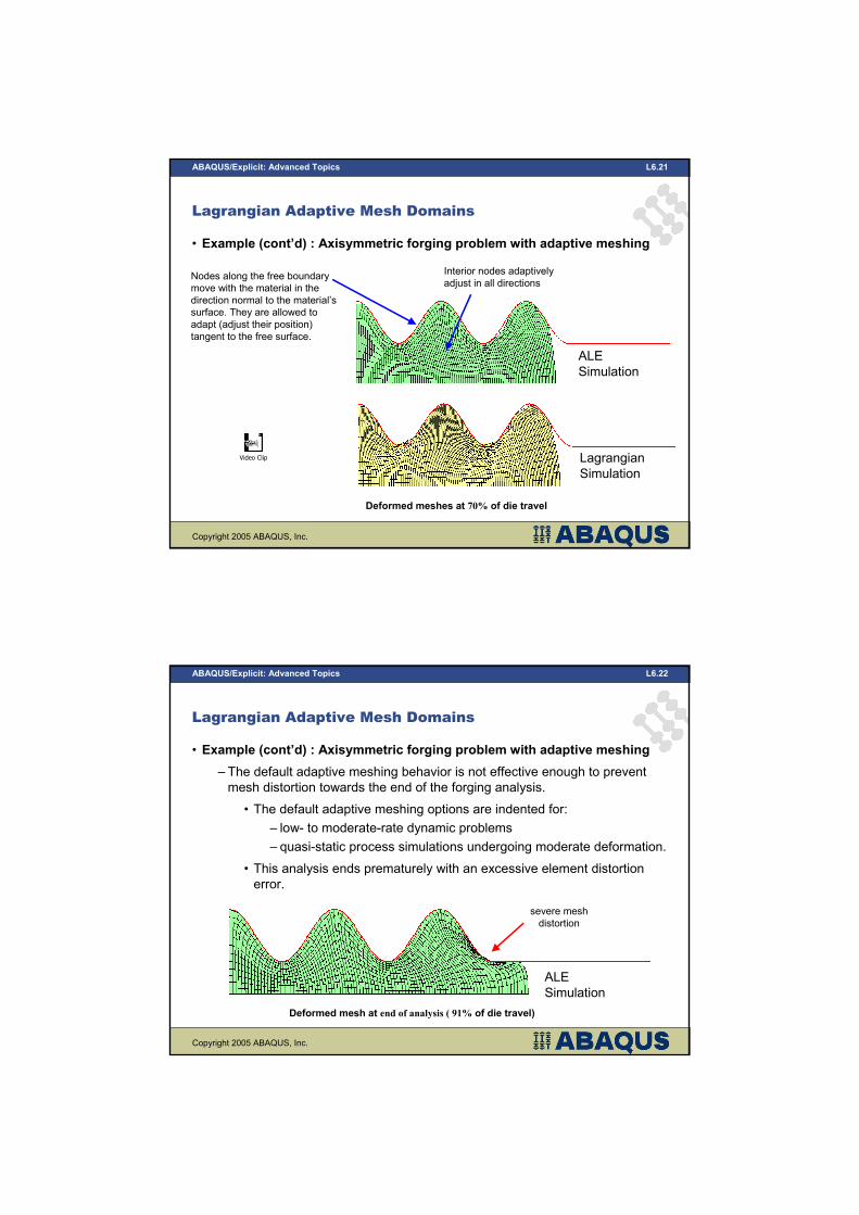
• Example (cont’d) : Axisymmetric forging problem with adaptive meshing
Lagrangian Adaptive Mesh Domains
Deformed meshes at 70% of die travel
Interior nodes adaptively
adjust in all directionsNodes along the free boundary
move with the material in the
direction normal to the material’s
surface. They are allowed to
adapt (adjust their position)
tangent to the free surface.
ALE
Simulation
Lagrangian
Simulation
Video Clip
Copyright 2005 ABAQUS, Inc.
ABAQUS/Explicit: Advanced Topics L6.22
Lagrangian Adaptive Mesh Domains
• Example (cont’d) : Axisymmetric forging problem with adaptive meshing
– The default adaptive meshing behavior is not effective enough to prevent
mesh distortion towards the end of the forging analysis.
• The default adaptive meshing options are indented for:
– low- to moderate-rate dynamic problems
– quasi-static process simulations undergoing moderate deformation.
• This analysis ends prematurely with an excessive element distortion
error.
Deformed mesh at end of analysis ( 91% of die travel)
ALE
Simulation
severe mesh
distortion
Copyright 2005 ABAQUS, Inc.
ABAQUS/Explicit: Advanced Topics L6.23
Lagrangian Adaptive Mesh Domains
• Frequency of adaptive meshing
– In most cases the frequency of adaptive meshing is the parameter that
most affects the mesh quality and the computational efficiency of adaptive
meshing.
• The default for Lagrangian (transient) problems, is for an adaptive
mesh increment to be performed after every 10 “explicit” increments.
• If the entire model acts as the adaptive mesh domain, each adaptive
meshing increment costs about the same as 3–5 “explicit” increments.
– In an adaptive meshing increment, ABAQUS/Explicit creates a new
smoother mesh by sweeping iteratively over the adaptive mesh domain.
• During each sweep, nodes are adjusted slightly to reduce element
distortion.
• By default, 1 mesh sweep is performed per adaptive mesh increment.
Copyright 2005 ABAQUS, Inc.
ABAQUS/Explicit: Advanced Topics L6.24
Lagrangian Adaptive Mesh Domains
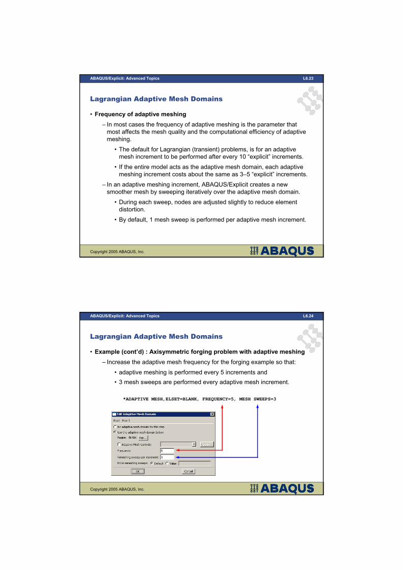
• Example (cont’d) : Axisymmetric forging problem with adaptive meshing
– Increase the adaptive mesh frequency for the forging example so that:
• adaptive meshing is performed every 5 increments and
• 3 mesh sweeps are performed every adaptive mesh increment.
*ADAPTIVE MESH,ELSET=BLANK, FREQUENCY=5, MESH SWEEPS=3
Copyright 2005 ABAQUS, Inc.
ABAQUS/Explicit: Advanced Topics L6.25
Lagrangian Adaptive Mesh Domains
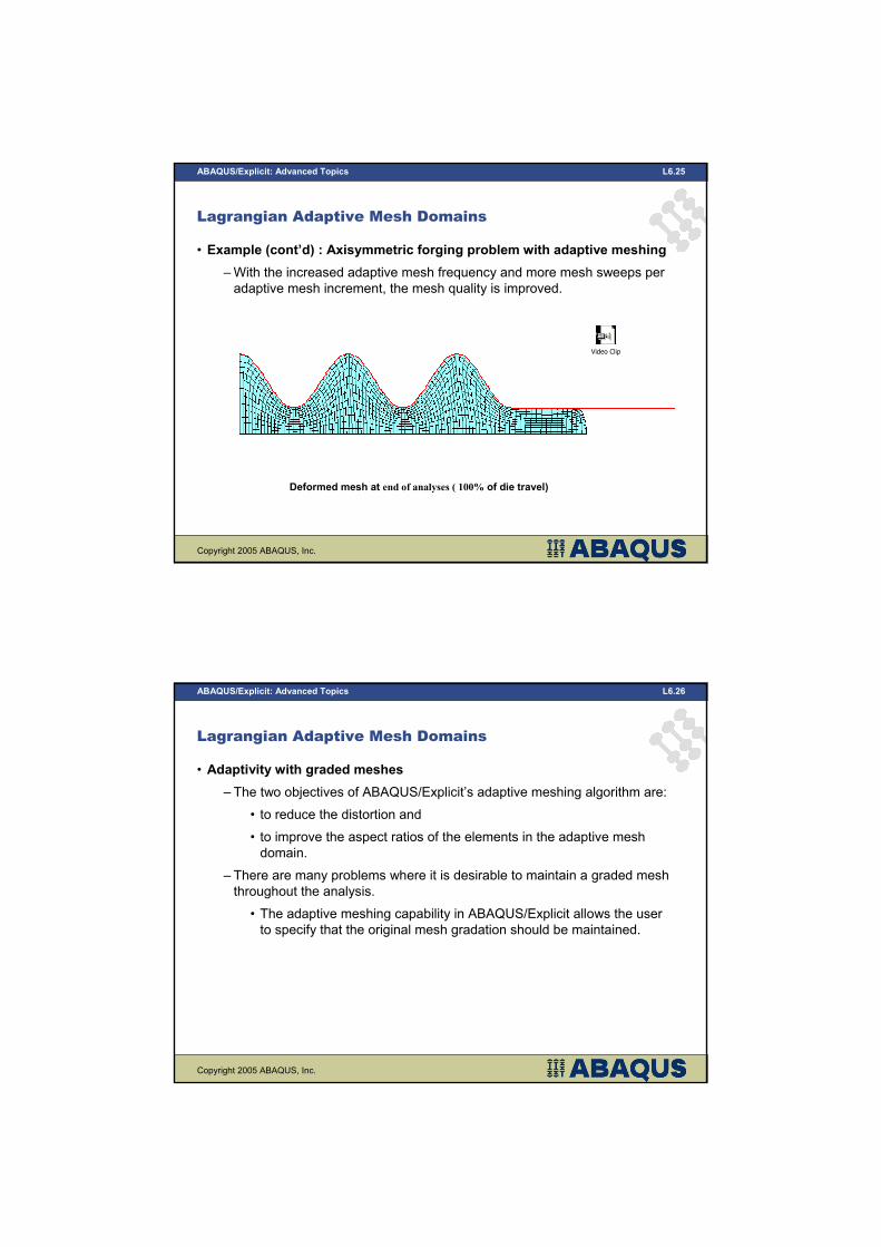
• Example (cont’d) : Axisymmetric forging problem with adaptive meshing
–With the increased adaptive mesh frequency and more mesh sweeps per
adaptive mesh increment, the mesh quality is improved.
Deformed mesh at end of analyses ( 100% of die travel)
Video Clip
Copyright 2005 ABAQUS, Inc.
ABAQUS/Explicit: Advanced Topics L6.26
Lagrangian Adaptive Mesh Domains
• Adaptivity with graded meshes
– The two objectives of ABAQUS/Explicit’s adaptive meshing algorithm are:
• to reduce the distortion and
• to improve the aspect ratios of the elements in the adaptive mesh
domain.
– There are many problems where it is desirable to maintain a graded mesh
throughout the analysis.
• The adaptive meshing capability in ABAQUS/Explicit allows the user
to specify that the original mesh gradation should be maintained.
Copyright 2005 ABAQUS, Inc.
ABAQUS/Explicit: Advanced Topics L6.27
Lagrangian Adaptive Mesh Domains
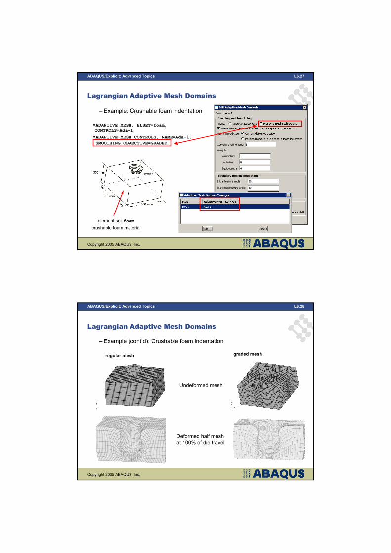
– Example: Crushable foam indentation
*ADAPTIVE MESH, ELSET=foam,
CONTROLS=Ada-1
*ADAPTIVE MESH CONTROLS, NAME=Ada-1,
SMOOTHING OBJECTIVE=GRADED
element set foam
crushable foam material
Copyright 2005 ABAQUS, Inc.
ABAQUS/Explicit: Advanced Topics L6.28
Lagrangian Adaptive Mesh Domains
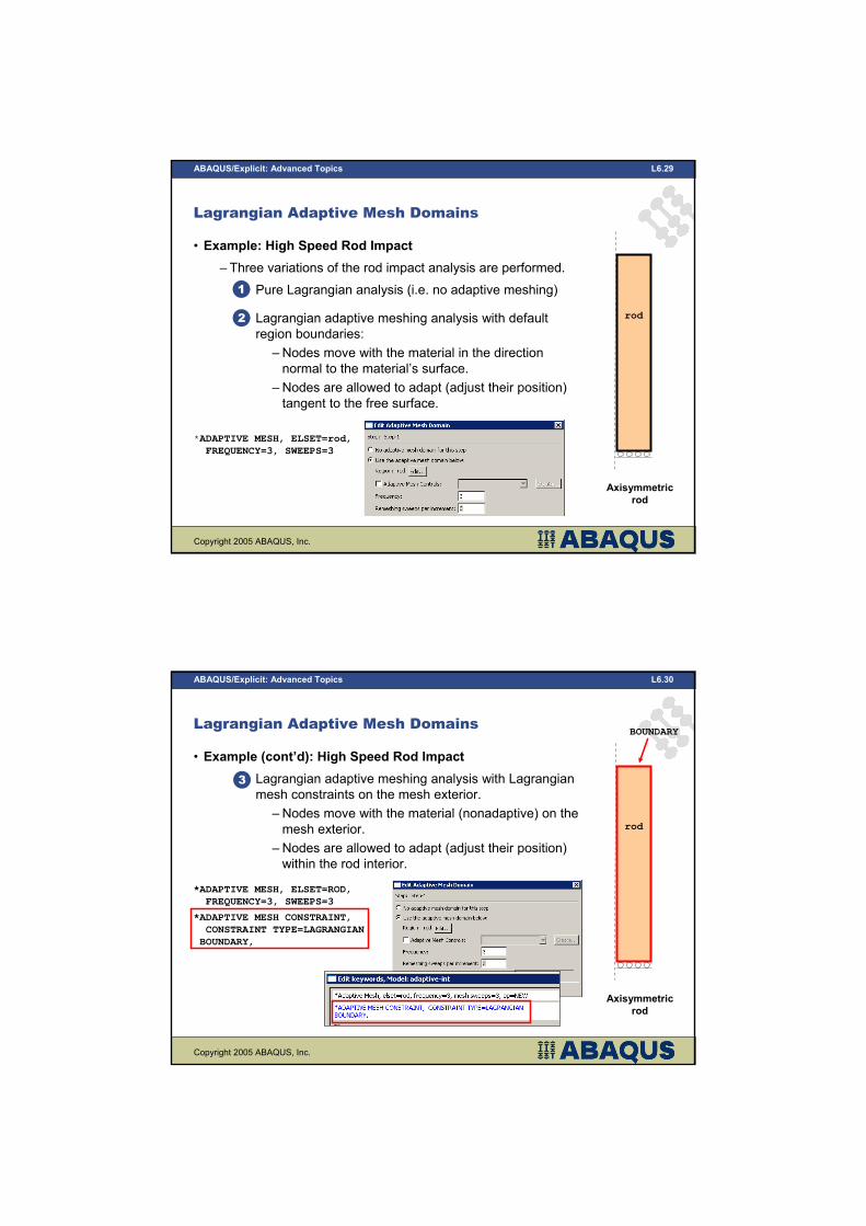
– Example (cont’d): Crushable foam indentation
Deformed half mesh
at 100% of die travel
regular mesh graded mesh
Undeformed mesh
Copyright 2005 ABAQUS, Inc.
ABAQUS/Explicit: Advanced Topics L6.29
Lagrangian Adaptive Mesh Domains
• Example: High Speed Rod Impact
– Three variations of the rod impact analysis are performed.
• Pure Lagrangian analysis (i.e. no adaptive meshing)
• Lagrangian adaptive meshing analysis with default
region boundaries:
– Nodes move with the material in the direction
normal to the material’s surface.
– Nodes are allowed to adapt (adjust their position)
tangent to the free surface.
*ADAPTIVE MESH, ELSET=rod,
FREQUENCY=3, SWEEPS=3
Axisymmetric
rod
1
2 rod
Copyright 2005 ABAQUS, Inc.
ABAQUS/Explicit: Advanced Topics L6.30
Lagrangian Adaptive Mesh Domains
• Example (cont’d): High Speed Rod Impact
• Lagrangian adaptive meshing analysis with Lagrangian
mesh constraints on the mesh exterior.
– Nodes move with the material (nonadaptive) on the
mesh exterior.
– Nodes are allowed to adapt (adjust their position)
within the rod interior.
*ADAPTIVE MESH, ELSET=ROD,
FREQUENCY=3, SWEEPS=3
*ADAPTIVE MESH CONSTRAINT,
CONSTRAINT TYPE=LAGRANGIAN
BOUNDARY,
rod
3
BOUNDARY
Axisymmetric
rod
Copyright 2005 ABAQUS, Inc.
ABAQUS/Explicit: Advanced Topics L6.31
Lagrangian Adaptive Mesh Domains
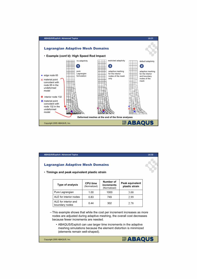
• Example (cont’d): High Speed Rod Impact
Deformed meshes at the end of the three analyses
edge node 65
material point
coincident with
node 65 in the
undeformed
model
interior node 132
material point
coincident with
node 132 in the
undeformed
model
pure
Lagrangian
formulation
1
no adaptivity
adaptive meshing
for the interior
nodes of the mesh
only
3
restricted adaptivity
2
adaptive meshing
for the interior
and boundary
nodes of the
mesh
default adaptivity
Copyright 2005 ABAQUS, Inc.
ABAQUS/Explicit: Advanced Topics L6.32
Lagrangian Adaptive Mesh Domains
• Timings and peak equivalent plastic strain
– This example shows that while the cost per increment increases as more
nodes are adjusted during adaptive meshing, the overall cost decreases
because fewer increments are needed.
• ABAQUS/Explicit can use larger time increments in the adaptive
meshing simulations because the element distortion is minimized
(elements remain well-shaped).
2.783020.44ALE for interior and
boundary nodes
2.997490.83ALE for interior nodes
3.0010001.00Pure Lagrangian
Peak equivalent
plastic strain
Number of
increments (Normalized)
CPU time (Normalized)
Type of analysis
Copyright 2005 ABAQUS, Inc.
ABAQUS/Explicit: Advanced Topics
Eulerian Adaptive Mesh Domains for
Steady-state Analyses
Copyright 2005 ABAQUS, Inc.
ABAQUS/Explicit: Advanced Topics L6.34
Eulerian Adaptive Mesh Domains for Steady-state
Analyses
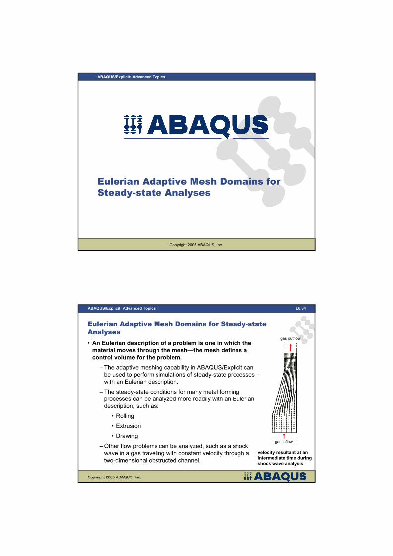
• An Eulerian description of a problem is one in which the
material moves through the mesh—the mesh defines a
control volume for the problem.
– The adaptive meshing capability in ABAQUS/Explicit can
be used to perform simulations of steady-state processes
with an Eulerian description.
– The steady-state conditions for many metal forming
processes can be analyzed more readily with an Eulerian
description, such as:
• Rolling
• Extrusion
• Drawing
–Other flow problems can be analyzed, such as a shock
wave in a gas traveling with constant velocity through a
two-dimensional obstructed channel.
velocity resultant at an
intermediate time during
shock wave analysis
gas inflow
gas outflow
Copyright 2005 ABAQUS, Inc.
ABAQUS/Explicit: Advanced Topics L6.35
Eulerian Adaptive Mesh Domains for Steady-state
Analyses
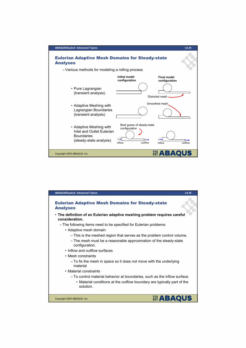
– Various methods for modeling a rolling process
• Pure Lagrangian
(transient analysis)
• Adaptive Meshing with
Lagrangian Boundaries
(transient analysis)
• Adaptive Meshing with
Inlet and Outlet Eulerian
Boundaries
(steady-state analysis)
Best guess of steady-state
configuration
Initial model
configurationFinal model
configuration
Distorted mesh
Smoothed mesh
inflow outflow inflow outflow
Copyright 2005 ABAQUS, Inc.
ABAQUS/Explicit: Advanced Topics L6.36
Eulerian Adaptive Mesh Domains for Steady-state
Analyses
• The definition of an Eulerian adaptive meshing problem requires careful
consideration.
– The following items need to be specified for Eulerian problems:
• Adaptive mesh domain
– This is the meshed region that serves as the problem control volume.
– The mesh must be a reasonable approximation of the steady-state
configuration.
• Inflow and outflow surfaces
• Mesh constraints
– To fix the mesh in space so it does not move with the underlying
material
• Material constraints
– To control material behavior at boundaries, such as the inflow surface.
• Material conditions at the outflow boundary are typically part of the
solution.
Copyright 2005 ABAQUS, Inc.
ABAQUS/Explicit: Advanced Topics L6.37
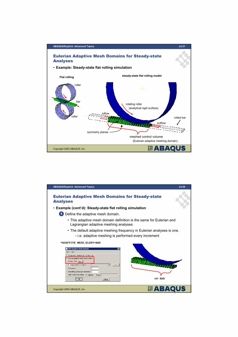
• Example: Steady-state flat rolling simulation
Eulerian Adaptive Mesh Domains for Steady-state
Analyses
inflow
outflow
rotating roller
(analytical rigid surface)
symmetry planes
meshed control volume
(Eulerian adaptive meshing domain)
rolled bar
steady-state flat rolling modelFlat rolling
roller
roller
bar
Copyright 2005 ABAQUS, Inc.
ABAQUS/Explicit: Advanced Topics L6.38
Eulerian Adaptive Mesh Domains for Steady-state
Analyses
• Example (cont’d): Steady-state flat rolling simulation
– Define the adaptive mesh domain.
• This adaptive mesh domain definition is the same for Eulerian and
Lagrangian adaptive meshing analyses.
• The default adaptive meshing frequency in Eulerian analyses is one.
– i.e. adaptive meshing is performed every increment
*ADAPTIVE MESH,ELSET=BAR
1
set BAR
Copyright 2005 ABAQUS, Inc.
ABAQUS/Explicit: Advanced Topics L6.39
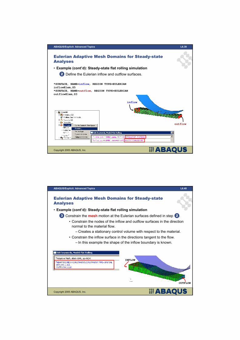
• Example (cont’d): Steady-state flat rolling simulation
– Define the Eulerian inflow and outflow surfaces.
*SURFACE, NAME=inflow, REGION TYPE=EULERIAN
inflowElem,S5
*SURFACE, NAME=outflow, REGION TYPE=EULERIAN
outflowElem,S3
2
Eulerian Adaptive Mesh Domains for Steady-state
Analyses
inflow
outflow
Copyright 2005 ABAQUS, Inc.
ABAQUS/Explicit: Advanced Topics L6.40
Eulerian Adaptive Mesh Domains for Steady-state
Analyses
• Example (cont’d): Steady-state flat rolling simulation
– Constrain the mesh motion at the Eulerian surfaces defined in step .
• Constrain the nodes of the inflow and outflow surfaces in the direction
normal to the material flow.
– Creates a stationary control volume with respect to the material.
• Constrain the inflow surface in the directions tangent to the flow.
– In this example the shape of the inflow boundary is known.
3 2
INFLOW
OUTFLOW
Copyright 2005 ABAQUS, Inc.
ABAQUS/Explicit: Advanced Topics L6.41
Eulerian Adaptive Mesh Domains for Steady-state
Analyses
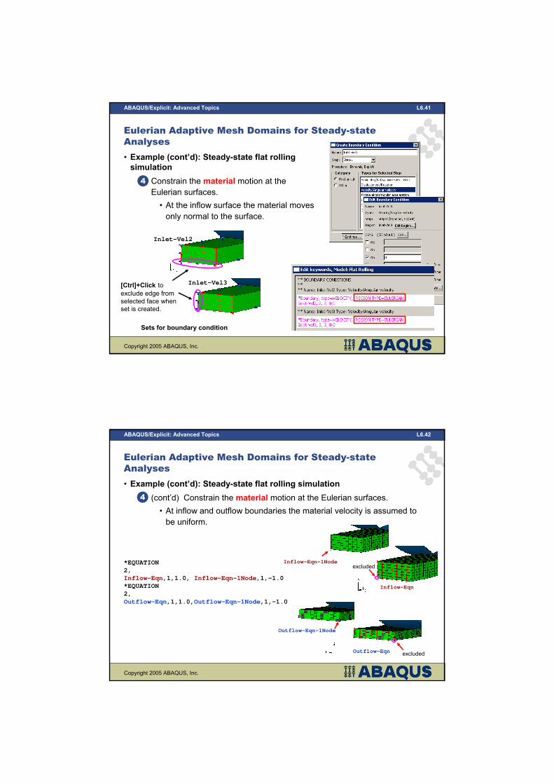
• Example (cont’d): Steady-state flat rolling
simulation
– Constrain the material motion at the
Eulerian surfaces.
• At the inflow surface the material moves
only normal to the surface.
4
Inlet-Vel3
Inlet-Vel2
[Ctrl]+Click to
exclude edge from
selected face when
set is created.
Sets for boundary condition
Copyright 2005 ABAQUS, Inc.
ABAQUS/Explicit: Advanced Topics L6.42
• Example (cont’d): Steady-state flat rolling simulation
– (cont’d) Constrain the material motion at the Eulerian surfaces.
• At inflow and outflow boundaries the material velocity is assumed to
be uniform.
*EQUATION
2,
Inflow-Eqn,1,1.0, Inflow-Eqn-1Node,1,-1.0
*EQUATION
2,
Outflow-Eqn,1,1.0,Outflow-Eqn-1Node,1,-1.0
Eulerian Adaptive Mesh Domains for Steady-state
Analyses
4
Outflow-Eqn-1Node
Outflow-Eqnexcluded
Inflow-Eqn-1Nodeexcluded
Inflow-Eqn
Copyright 2005 ABAQUS, Inc.
ABAQUS/Explicit: Advanced Topics L6.43
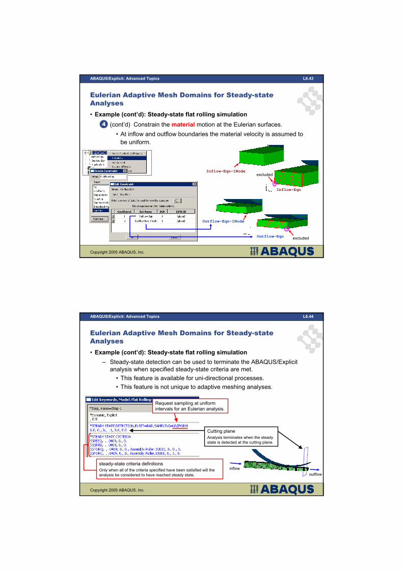
• Example (cont’d): Steady-state flat rolling simulation
– (cont’d) Constrain the material motion at the Eulerian surfaces.
• At inflow and outflow boundaries the material velocity is assumed to
be uniform.
Eulerian Adaptive Mesh Domains for Steady-state
Analyses
4
Outflow-Eqn-1Node
Outflow-Eqnexcluded
Inflow-Eqn-1Nodeexcluded
Inflow-Eqn
Copyright 2005 ABAQUS, Inc.
ABAQUS/Explicit: Advanced Topics L6.44
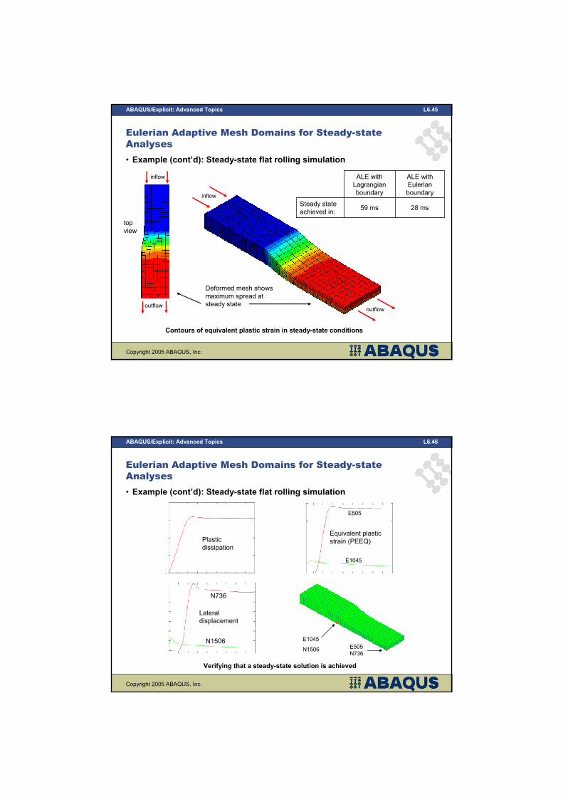
• Example (cont’d): Steady-state flat rolling simulation
– Steady-state detection can be used to terminate the ABAQUS/Explicit
analysis when specified steady-state criteria are met.
• This feature is available for uni-directional processes.
• This feature is not unique to adaptive meshing analyses.
Eulerian Adaptive Mesh Domains for Steady-state
Analyses
Request sampling at uniform
intervals for an Eulerian analysis.
Cutting plane
Analysis terminates when the steady
state is detected at the cutting plane.
outflow
inflowsteady-state criteria definitions
Only when all of the criteria specified have been satisfied will the
analysis be considered to have reached steady state.
Copyright 2005 ABAQUS, Inc.
ABAQUS/Explicit: Advanced Topics L6.45
• Example (cont’d): Steady-state flat rolling simulation
Eulerian Adaptive Mesh Domains for Steady-state
Analyses
Steady state
achieved in:28 ms59 ms
ALE with
Eulerian
boundary
ALE with
Lagrangian
boundary
Contours of equivalent plastic strain in steady-state conditions
top
view
inflow
outflow
inflow
outflow
Deformed mesh shows
maximum spread at
steady state
Copyright 2005 ABAQUS, Inc.
ABAQUS/Explicit: Advanced Topics L6.46
E1045
N1506E505
N736
Eulerian Adaptive Mesh Domains for Steady-state
Analyses
Verifying that a steady-state solution is achieved
N736
N1506
Lateral
displacement
E505
E1045
Equivalent plastic
strain (PEEQ)Plastic
dissipation
• Example (cont’d): Steady-state flat rolling simulation
Copyright 2005 ABAQUS, Inc.
ABAQUS/Explicit: Advanced Topics L6.47
Eulerian Adaptive Mesh Domains for Steady-state
Analyses
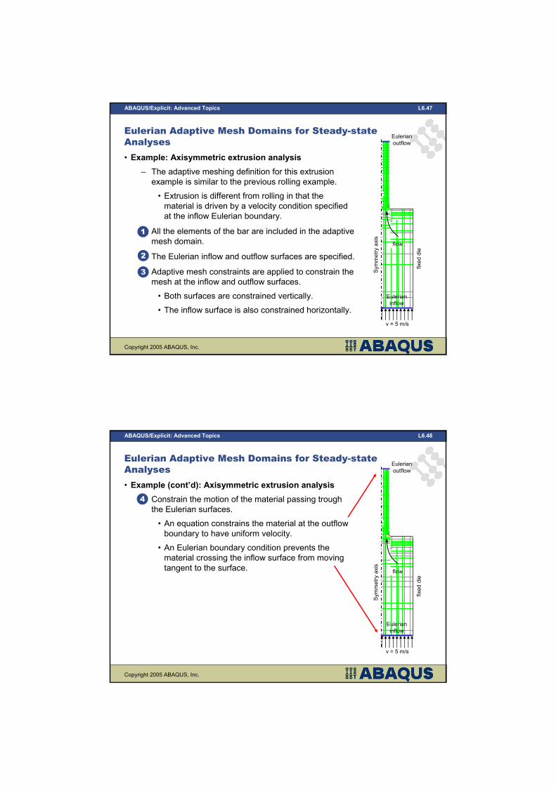
• Example: Axisymmetric extrusion analysis
– The adaptive meshing definition for this extrusion
example is similar to the previous rolling example.
• Extrusion is different from rolling in that the
material is driven by a velocity condition specified
at the inflow Eulerian boundary.
– All the elements of the bar are included in the adaptive
mesh domain.
– The Eulerian inflow and outflow surfaces are specified.
– Adaptive mesh constraints are applied to constrain the
mesh at the inflow and outflow surfaces.
• Both surfaces are constrained vertically.
• The inflow surface is also constrained horizontally.
1
fixed die
Symmetry axis
flow
v = 5 m/s
Eulerian
inflow
Eulerian
outflow
2
3
Copyright 2005 ABAQUS, Inc.
ABAQUS/Explicit: Advanced Topics L6.48
Eulerian Adaptive Mesh Domains for Steady-state
Analyses
• Example (cont’d): Axisymmetric extrusion analysis
– Constrain the motion of the material passing trough
the Eulerian surfaces.
• An equation constrains the material at the outflow
boundary to have uniform velocity.
• An Eulerian boundary condition prevents the
material crossing the inflow surface from moving
tangent to the surface.
4
fixed die
Symmetry axis
flow
v = 5 m/s
Eulerian
inflow
Eulerian
outflow
Copyright 2005 ABAQUS, Inc.
ABAQUS/Explicit: Advanced Topics L6.49
Eulerian Adaptive Mesh Domains for Steady-state
Analyses
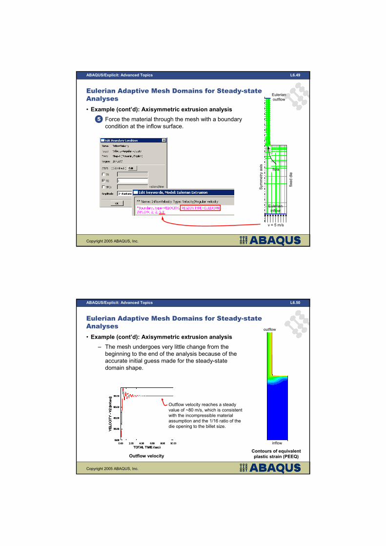
• Example (cont’d): Axisymmetric extrusion analysis
– Force the material through the mesh with a boundary
condition at the inflow surface.
5
fixed die
Symmetry axis
flow
v = 5 m/s
Eulerian
inflow
Eulerian
outflow
Copyright 2005 ABAQUS, Inc.
ABAQUS/Explicit: Advanced Topics L6.50
Eulerian Adaptive Mesh Domains for Steady-state
Analyses
• Example (cont’d): Axisymmetric extrusion analysis
– The mesh undergoes very little change from the
beginning to the end of the analysis because of the
accurate initial guess made for the steady-state
domain shape.
inflow
outflow
Contours of equivalent
plastic strain (PEEQ)
Outflow velocity reaches a steady
value of ~80 m/s, which is consistent
with the incompressible material
assumption and the 1/16 ratio of the
die opening to the billet size.
Outflow velocity
Copyright 2005 ABAQUS, Inc.
ABAQUS/Explicit: Advanced Topics
Adaptive Meshing Output and
Diagnostics
Copyright 2005 ABAQUS, Inc.
ABAQUS/Explicit: Advanced Topics L6.52
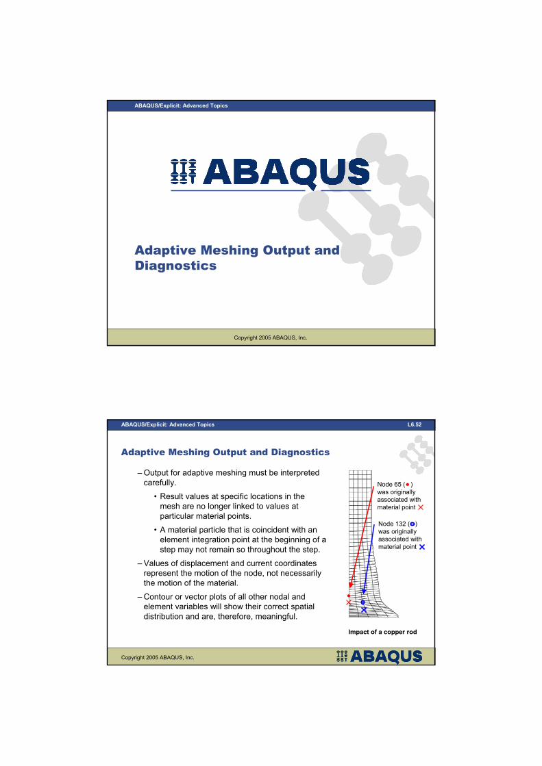
Adaptive Meshing Output and Diagnostics
–Output for adaptive meshing must be interpreted
carefully.
• Result values at specific locations in the
mesh are no longer linked to values at
particular material points.
• A material particle that is coincident with an
element integration point at the beginning of a
step may not remain so throughout the step.
– Values of displacement and current coordinates
represent the motion of the node, not necessarily
the motion of the material.
– Contour or vector plots of all other nodal and
element variables will show their correct spatial
distribution and are, therefore, meaningful.
Node 65 ( )
was originally
associated with
material point
Node 132 ( )
was originally
associated with
material point
Impact of a copper rod
Copyright 2005 ABAQUS, Inc.
ABAQUS/Explicit: Advanced Topics L6.53
Adaptive Meshing Output and Diagnostics
• Tracer particles
– Tracer particles can be defined to track material points in an adaptive
mesh domain.
• These particles can also be used to obtain time histories that
correspond to the time variation at a specific material point.
– Output for tracer particles can be written only to the output database file.
• They can be viewed in ABAQUS/Viewer.Tracer particles will leave
their parent nodes 5
times during the step
– The initial location of a tracer
particle is defined to be coincident
with a node, termed the parent
node.
– Sets of tracer particles can be
released from the current
locations of the parent nodes at
multiple times during the step.
Make specific output
requests for the
defined tracer set
Copyright 2005 ABAQUS, Inc.
ABAQUS/Explicit: Advanced Topics L6.54
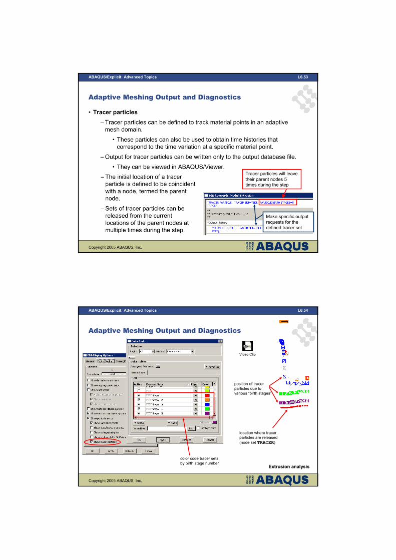
Adaptive Meshing Output and Diagnostics
Video Clip
position of tracer
particles due to
various “birth stages”
location where tracer
particles are released
(node set TRACER)
color code tracer sets
by birth stage numberExtrusion analysis
Copyright 2005 ABAQUS, Inc.
ABAQUS/Explicit: Advanced Topics L6.55
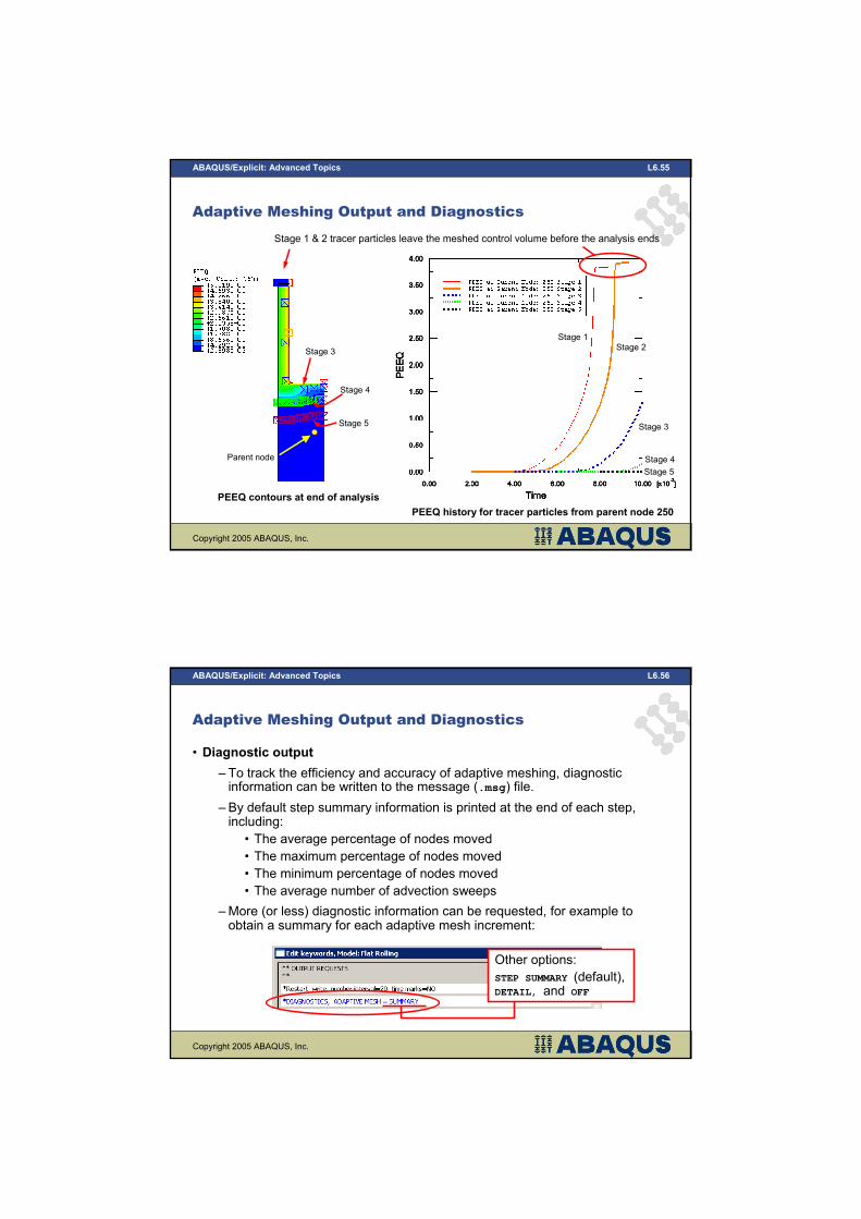
Adaptive Meshing Output and Diagnostics
PEEQ history for tracer particles from parent node 250
PEEQ contours at end of analysis
Parent node
Stage 3
Stage 4
Stage 5
Stage 1
Stage 5
Stage 4
Stage 2
Stage 3
Stage 1 & 2 tracer particles leave the meshed control volume before the analysis ends
Copyright 2005 ABAQUS, Inc.
ABAQUS/Explicit: Advanced Topics L6.56
• Diagnostic output
– To track the efficiency and accuracy of adaptive meshing, diagnostic information can be written to the message (.msg) file.
– By default step summary information is printed at the end of each step, including:
• The average percentage of nodes moved
• The maximum percentage of nodes moved
• The minimum percentage of nodes moved
• The average number of advection sweeps
–More (or less) diagnostic information can be requested, for example to obtain a summary for each adaptive mesh increment:
Adaptive Meshing Output and Diagnostics
Other options:
STEP SUMMARY (default),DETAIL, and OFF
Copyright 2005 ABAQUS, Inc.
ABAQUS/Explicit: Advanced Topics
Additional Features of Adaptive
Meshing
Copyright 2005 ABAQUS, Inc.
ABAQUS/Explicit: Advanced Topics L6.58
Additional Features of Adaptive Meshing
• Adaptive mesh Boundary Regions
– Adaptive mesh boundary regions bound the adaptive mesh domain:
• Surfaces in three dimensional problems
• Edges in two-dimensional problems
– ABAQUS/Explicit will create adaptive mesh boundary regions on:
• The exterior of a model
• The boundary between different adaptive mesh domains
• The boundary between an adaptive mesh domain and a nonadaptive
domain
– You can define adaptive mesh boundary regions using
• Boundary conditions
• Loads (concentrated and distributed)
• Surface definitions
Copyright 2005 ABAQUS, Inc.
ABAQUS/Explicit: Advanced Topics L6.59
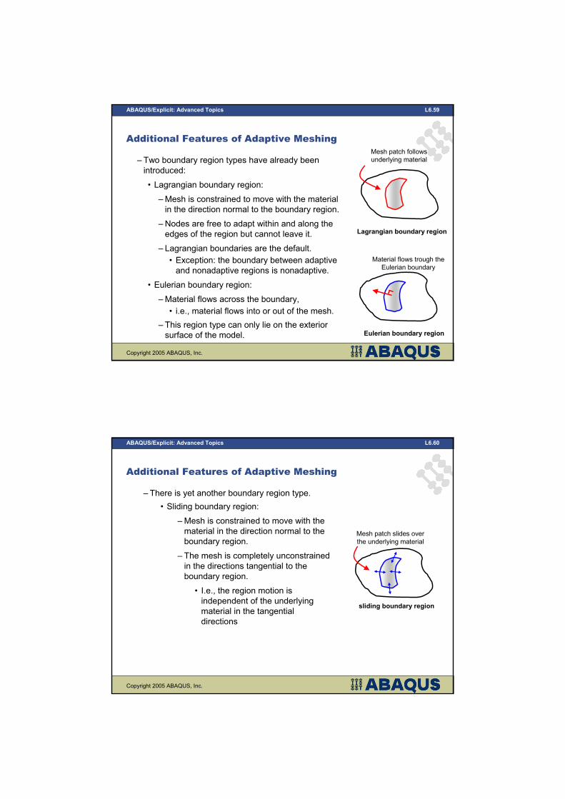
Additional Features of Adaptive Meshing
– Two boundary region types have already been
introduced:
• Lagrangian boundary region:
– Mesh is constrained to move with the material
in the direction normal to the boundary region.
– Nodes are free to adapt within and along the
edges of the region but cannot leave it.
– Lagrangian boundaries are the default.
• Exception: the boundary between adaptive
and nonadaptive regions is nonadaptive.
• Eulerian boundary region:
– Material flows across the boundary,
• i.e., material flows into or out of the mesh.
– This region type can only lie on the exterior
surface of the model.
Lagrangian boundary region
Mesh patch follows
underlying material
Eulerian boundary region
Material flows trough the
Eulerian boundary
Copyright 2005 ABAQUS, Inc.
ABAQUS/Explicit: Advanced Topics L6.60
Additional Features of Adaptive Meshing
– There is yet another boundary region type.
• Sliding boundary region:
– Mesh is constrained to move with the
material in the direction normal to the
boundary region.
– The mesh is completely unconstrained
in the directions tangential to the
boundary region.
• I.e., the region motion is
independent of the underlying
material in the tangential
directions
sliding boundary region
Mesh patch slides over
the underlying material
Copyright 2005 ABAQUS, Inc.
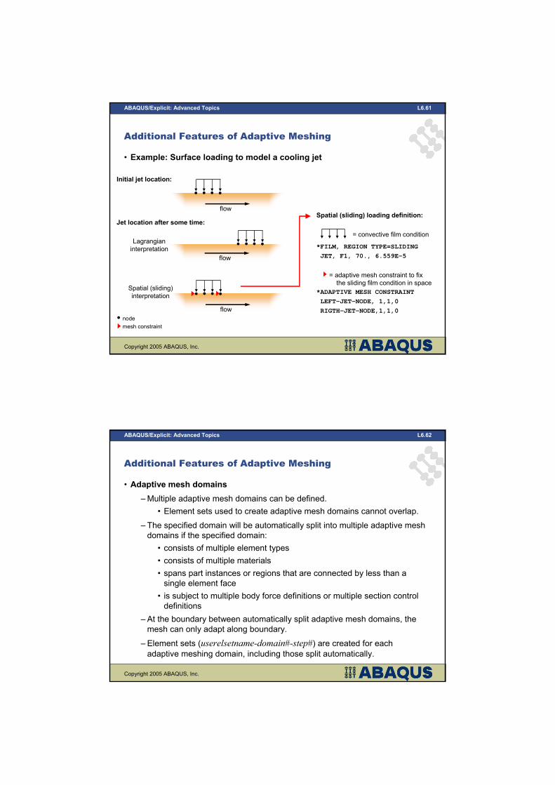
ABAQUS/Explicit: Advanced Topics L6.61
• Example: Surface loading to model a cooling jet
Additional Features of Adaptive Meshing
flow
Initial jet location:
Jet location after some time:
flow
flow
Lagrangian
interpretation
mesh constraint
node
Spatial (sliding)
interpretation
Spatial (sliding) loading definition:
= convective film condition
*FILM, REGION TYPE=SLIDING
JET, F1, 70., 6.559E-5
= adaptive mesh constraint to fix
the sliding film condition in space
*ADAPTIVE MESH CONSTRAINT
LEFT-JET-NODE, 1,1,0
RIGTH-JET-NODE,1,1,0
Copyright 2005 ABAQUS, Inc.
ABAQUS/Explicit: Advanced Topics L6.62
Additional Features of Adaptive Meshing
• Adaptive mesh domains
–Multiple adaptive mesh domains can be defined.
• Element sets used to create adaptive mesh domains cannot overlap.
– The specified domain will be automatically split into multiple adaptive mesh
domains if the specified domain:
• consists of multiple element types
• consists of multiple materials
• spans part instances or regions that are connected by less than a
single element face
• is subject to multiple body force definitions or multiple section control
definitions
– At the boundary between automatically split adaptive mesh domains, the
mesh can only adapt along boundary.
– Element sets (userelsetname-domain#-step#) are created for each adaptive meshing domain, including those split automatically.
Copyright 2005 ABAQUS, Inc.
ABAQUS/Explicit: Advanced Topics L6.63
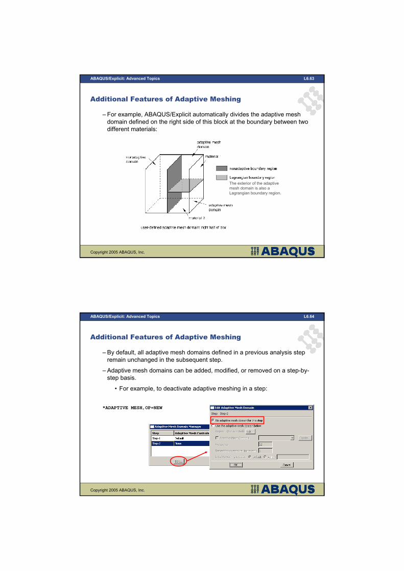
Additional Features of Adaptive Meshing
– For example, ABAQUS/Explicit automatically divides the adaptive mesh
domain defined on the right side of this block at the boundary between two
different materials:
The exterior of the adaptive
mesh domain is also a
Lagrangian boundary region.
Copyright 2005 ABAQUS, Inc.
ABAQUS/Explicit: Advanced Topics L6.64
Additional Features of Adaptive Meshing
– By default, all adaptive mesh domains defined in a previous analysis step
remain unchanged in the subsequent step.
– Adaptive mesh domains can be added, modified, or removed on a step-by-
step basis.
• For example, to deactivate adaptive meshing in a step:
*ADAPTIVE MESH,OP=NEW
Copyright 2005 ABAQUS, Inc.
ABAQUS/Explicit: Advanced Topics L6.65
Additional Features of Adaptive Meshing
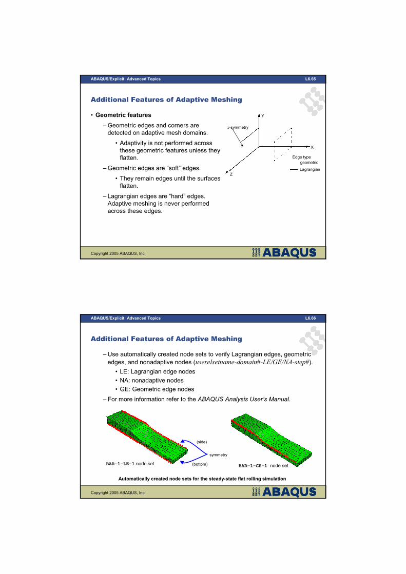
• Geometric features
–Geometric edges and corners are
detected on adaptive mesh domains.
• Adaptivity is not performed across
these geometric features unless they
flatten.
– Geometric edges are “soft” edges.
• They remain edges until the surfaces
flatten.
– Lagrangian edges are “hard” edges.
Adaptive meshing is never performed
across these edges.
Lagrangian
geometric
Y
Z
X
x-symmetry
Edge type
Copyright 2005 ABAQUS, Inc.
ABAQUS/Explicit: Advanced Topics L6.66
Additional Features of Adaptive Meshing
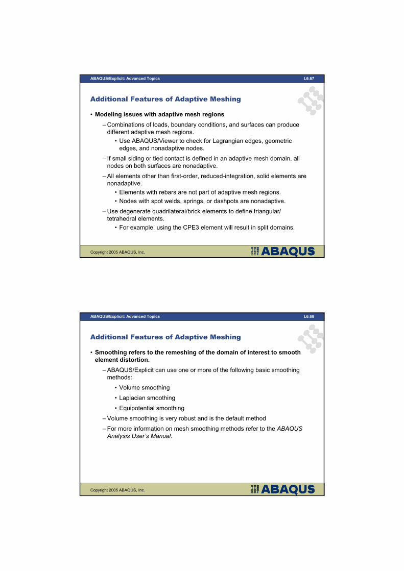
– Use automatically created node sets to verify Lagrangian edges, geometric
edges, and nonadaptive nodes (userelsetname-domain#-LE/GE/NA-step#).
• LE: Lagrangian edge nodes
• NA: nonadaptive nodes
• GE: Geometric edge nodes
– For more information refer to the ABAQUS Analysis User’s Manual.
BAR-1-GE-1 node setBAR-1-LE-1 node set
symmetry
(bottom)
(side)
Automatically created node sets for the steady-state flat rolling simulation
Copyright 2005 ABAQUS, Inc.
ABAQUS/Explicit: Advanced Topics L6.67
Additional Features of Adaptive Meshing
• Modeling issues with adaptive mesh regions
– Combinations of loads, boundary conditions, and surfaces can produce
different adaptive mesh regions.
• Use ABAQUS/Viewer to check for Lagrangian edges, geometric
edges, and nonadaptive nodes.
– If small siding or tied contact is defined in an adaptive mesh domain, all
nodes on both surfaces are nonadaptive.
– All elements other than first-order, reduced-integration, solid elements are
nonadaptive.
• Elements with rebars are not part of adaptive mesh regions.
• Nodes with spot welds, springs, or dashpots are nonadaptive.
– Use degenerate quadrilateral/brick elements to define triangular/
tetrahedral elements.
• For example, using the CPE3 element will result in split domains.
Copyright 2005 ABAQUS, Inc.
ABAQUS/Explicit: Advanced Topics L6.68
Additional Features of Adaptive Meshing
• Smoothing refers to the remeshing of the domain of interest to smooth
element distortion.
– ABAQUS/Explicit can use one or more of the following basic smoothing
methods:
• Volume smoothing
• Laplacian smoothing
• Equipotential smoothing
– Volume smoothing is very robust and is the default method
– For more information on mesh smoothing methods refer to the ABAQUS
Analysis User’s Manual.
Copyright 2005 ABAQUS, Inc.
ABAQUS/Explicit: Advanced Topics L6.69
Additional Features of Adaptive Meshing
• After the mesh has been smoothed element variables, nodal variables,
and momentum are remapped by advection.
– Two advection methods are available in ABAQUS/Explicit:
• The default second-order advection method improves accuracy during
the remapping phase of adaptive meshing.
• First-order method tends to diffuse any sharp gradients of element
variables during the remapping phase.
– For more information on advection refer to the ABAQUS Analysis User’s
Manual.
Copyright 2005 ABAQUS, Inc.
ABAQUS/Explicit: Advanced Topics L6.70
Additional Features of Adaptive Meshing
• Solution-dependent adaptive meshing prevents the reduction of mesh
refinement near areas of evolving concave curvature.
– Basic smoothing methods reduce the mesh refinement near concave
boundaries.
–With solution-dependent adaptive meshing, mesh gradation is
automatically focused toward these areas.
• The aggressiveness of the meshing is governed by the curvature
refinement weight, which has a default value of 1.
– For more information refer to the ABAQUS Analysis User’s Manual.
Axisymmetric forging problemDefault curvature refinement No curvature refinement
Copyright 2005 ABAQUS, Inc.
ABAQUS/Explicit: Advanced Topics
Element Distortion Control
Copyright 2005 ABAQUS, Inc.
ABAQUS/Explicit: Advanced Topics L6.72
Element Distortion Control
• ABAQUS/Explicit offers distortion
control to prevent solid elements
from inverting or distorting
excessively.
– Distortion control is designed to
prevent negative element volumes
or other excessive distortion from
occurring during an analysis.
• In contrast to the adaptive
meshing technique, distortion
control does not attempt to
maintain a high-quality mesh
throughout an analysis.
• Elements with distortion control
can not be included in an
adaptive mesh domain.
no-dist-ctrl with dist ctrl
crushable foam indentation
Copyright 2005 ABAQUS, Inc.
ABAQUS/Explicit: Advanced Topics L6.73
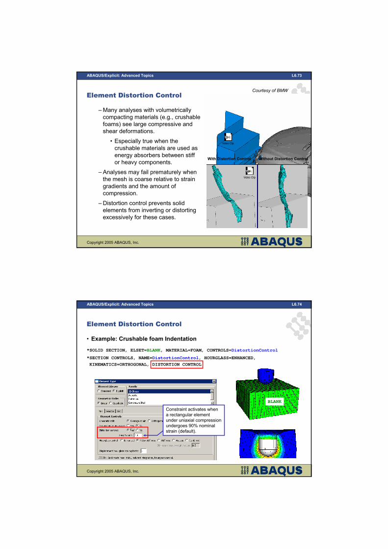
Element Distortion Control
–Many analyses with volumetrically
compacting materials (e.g., crushable
foams) see large compressive and
shear deformations.
• Especially true when the
crushable materials are used as
energy absorbers between stiff
or heavy components.
– Analyses may fail prematurely when
the mesh is coarse relative to strain
gradients and the amount of
compression.
– Distortion control prevents solid
elements from inverting or distorting
excessively for these cases.
Courtesy of BMW
Without Distortion ControlWith Distortion Control
Video Clip
Video Clip
Copyright 2005 ABAQUS, Inc.
ABAQUS/Explicit: Advanced Topics L6.74
Element Distortion Control
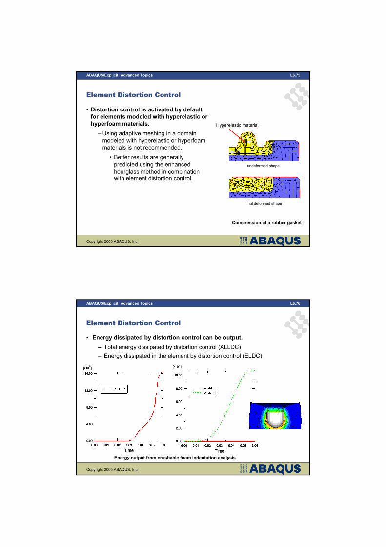
• Example: Crushable foam Indentation
*SOLID SECTION, ELSET=BLANK, MATERIAL=FOAM, CONTROLS=DistortionControl
*SECTION CONTROLS, NAME=DistortionControl, HOURGLASS=ENHANCED,
KINEMATICS=ORTHOGONAL, DISTORTION CONTROL
BLANK
Constraint activates when
a rectangular element
under uniaxial compression
undergoes 90% nominal
strain (default).
Copyright 2005 ABAQUS, Inc.
ABAQUS/Explicit: Advanced Topics L6.75
Element Distortion Control
• Distortion control is activated by default
for elements modeled with hyperelastic or
hyperfoam materials.
– Using adaptive meshing in a domain
modeled with hyperelastic or hyperfoam
materials is not recommended.
• Better results are generally
predicted using the enhanced
hourglass method in combination
with element distortion control.
final deformed shape
undeformed shape
Compression of a rubber gasket
Hyperelastic material
Copyright 2005 ABAQUS, Inc.
ABAQUS/Explicit: Advanced Topics L6.76
Element Distortion Control
• Energy dissipated by distortion control can be output.
– Total energy dissipated by distortion control (ALLDC)
– Energy dissipated in the element by distortion control (ELDC)
96
Energy output from crushable foam indentation analysis


![Topology-Adaptive Mesh Deformation for Surface Evolution, … · Topology-Adaptive Mesh Deformation for Surface Evolution, Morphing, and Multi-View Reconstruction. [Research Report]](https://img.pdfslide.net/doc/110x75/5f785df833d37a1d7d2d6044/topology-adaptive-mesh-deformation-for-surface-evolution-topology-adaptive-mesh.jpg)