Embed Size (px)
Citation preview
Helsinki University of Technology Signal Processing Laboratory
Teknillinen korkeakoulu Signaalinkäsittelytekniikan laboratorio
Espoo 2002 Report 36
ADAPTIVE METHODS FOR BLIND EQUALIZATION AND SIGNAL SEPARATION IN MIMO SYSTEMS Mihai Enescu Dissertation for the degree of Doctor of Science in Technology to be presented with due permission for public examination and debate in Auditorium S1 at Helsinki University of Technology (Espoo, Finland) on the 23rd of August, 2002, at 12 o’clock noon.
Helsinki University of Technology Department of Electrical and Communications Engineering Signal Processing Laboratory Teknillinen korkeakoulu Sähkö- ja tietoliikennetekniikan osasto Signaalinkäsittelytekniikan laboratorio

Distribution: Helsinki University of Technology Signal Processing Laboratory P.O. Box 3000 FIN-02015 HUT Tel. +358-9-451 2486 Fax. +358-9-460 224 E-mail: [email protected] Mihai Enescu ISBN 951-22-6042-5 ISSN 1456-6907 Otamedia Oy Espoo 2002
Abstract
This thesis addresses the problems of blind source separation (BSS) and blind and semi-blind
communications channel equalization. In blind source separation, signals from multiple sources
arrive simultaneously at a sensor array, so that each sensor output contains a mixture of source
signals. Sets of sensor outputs are processed to recover the source signals from the mixed obser-
vations. The termblind refers to the fact that specific source signal values and accurate parameter
values of a mixing model are not knowna priori. Application domains for the material in this
thesis include communications, biomedical, and sensor array signal processing.
The goal of this thesis is development of blind and semi-blind algorithms which require little
or no prior information about source signal or mixing system parameter values in order to process
the data. We start with the problem of extracting unknown input signals from measured outputs of
instantaneous multiple-input multiple-output (I-MIMO) systems with constant parameter values.
Suggested solutions are then extended to time-varying I-MIMO systems and also to constant
finite impulse response multiple-input multiple-output (FIR-MIMO) systems. Another goal is to
find a practical solution for the more challenging case of time-varying FIR-MIMO systems.
The source separation techniques proposed in this thesis are based on state-space models
and on recursive estimation. Blind separation algorithms based on Kalman filters are proposed.
The source signals are treated using low-order autoregressive models. Projections along signal
subspace eigenvectors are used to reduce the dimensionality of observations and also for spatial
decorrelation of sources. Any changes that occur in the signal subspace can be tracked on-
line. When considering slowly time-varying FIR-MIMO systems, fractional sampling can be
used to derive a set of slowly time-varying I-MIMO systems. Thus, the proposed recursive BSS
algorithms for I-MIMO systems can be used for blind equalization of slowly time-varying FIR
communications channels.
The problem of equalization of time-varying FIR MIMO systems is also addressed in this
thesis. The proposed solutions involve semi-blind algorithms which work in two stages. First,
a channel estimate is derived, and then the observation sequence is equalized. The algorithms
estimate the otherwise-unknown noise statistics, and as a result achieve performance close to
that of an optimal Kalman-based algorithm. A non-connected decision feedback equalization
algorithm is derived for FIR-MIMO systems, using a minimum mean square error criterion.
Simulation results show that the algorithm is able to track time and frequency selective channels
and also to mitigate intersymbol and interuser interference.
ii
Preface
The research work for this thesis was carried out at the Signal Processing Laboratory, Helsinki
University of Technology and the Signal Processing Laboratory, Tampere University of Technol-
ogy, during the years 1999-2001. I wish to express my gratitude to my supervisor, Prof. Visa
Koivunen, for his encouragement, guidance and support during the course of this work.
I would like to thank my thesis pre-examiners Prof. Ioan Tabus and Dr. Juha Laurila for
their constructive comments. I am also grateful to Prof. Iiro Hartimo, the director of Graduate
School in Electronics Telecommunications and Automation (GETA), to GETA secretary Marja
Leppaharju, and to our laboratory secretaries Anne J¨aaskelainen and Mirja Lemetyinen for help-
ing me with many practical issues and arrangements.
Many thanks to Dr. Charles Murphy for revising the language and for the great moments we
had in the U.S. and in Finland. I would like to thank Marius Sirbu, who co-authored several of my
publications. I am also grateful to my colleagues and co-workers, Dr. Yinglu Zhang, Dr. Samuli
Visuri, Jan Eriksson, Dr. Jukka Mannerkoski, Dr. Doru Giurcaneanu, Maarit Melvasalo, Juha
Karvanen, Timo Roman, Traian Abrudan, and Stefan Werner for our many interesting discus-
sions. Thanks are also due my friends in Helsinki and in Tampere with whom I spent wonderful
moments.
The financial support of the Academy of Finland, GETA, Nokia Foundation, Finnish Soci-
ety of Electronics Engineers Foundation, Tekniikan Edist¨amissaatio, Emil Aaltosen S¨aatio are
gratefully acknowledged.
I wish to give my deepest gratitude to my family, especially to my mother for her permanent
encouragement and support. Finally, I would like to thank my lovely fianc´ee Monica for love and
understanding during my time as a graduate student.
Otaniemi, June 2002
Mihai Enescu
iii

iv
Contents
Abstract i
Preface iii
List of publications ix
List of abbreviations and symbols xi
1 Introduction 1
1.1 Motivation. . . . . . . . . . . . . . . . . . . . . . . . . . . . . . . . . . . . . . 1
1.2 Scope of the thesis . .. . . . . . . . . . . . . . . . . . . . . . . . . . . . . . . 3
1.3 Contributions of the thesis . . . . .. . . . . . . . . . . . . . . . . . . . . . . . 4
1.4 Summary of publications . . . . . .. . . . . . . . . . . . . . . . . . . . . . . . 5
2 BSS model 9
2.1 Problem formulation and assumptions . . . . . .. . . . . . . . . . . . . . . . . 9
2.2 Key concepts in BSS .. . . . . . . . . . . . . . . . . . . . . . . . . . . . . . . 13
2.2.1 Contrast functions . . . . .. . . . . . . . . . . . . . . . . . . . . . . . 13
2.2.2 Score functions. . . . . . . . . . . . . . . . . . . . . . . . . . . . . . . 17
2.2.3 Estimating functions . . . .. . . . . . . . . . . . . . . . . . . . . . . . 17
2.3 Different classes of algorithms . . .. . . . . . . . . . . . . . . . . . . . . . . . 18
2.4 Blind Deconvolution .. . . . . . . . . . . . . . . . . . . . . . . . . . . . . . . 21
2.5 Applications of BSS .. . . . . . . . . . . . . . . . . . . . . . . . . . . . . . . 22
v
3 Adaptive Whitening 25
3.1 Introduction . . . . .. . . . . . . . . . . . . . . . . . . . . . . . . . . . . . . . 25
3.2 Subspace Tracking .. . . . . . . . . . . . . . . . . . . . . . . . . . . . . . . . 26
3.2.1 PAST and PASTd . . . . .. . . . . . . . . . . . . . . . . . . . . . . . . 27
3.2.2 Subspace tracking by subspace averaging . . .. . . . . . . . . . . . . . 29
3.2.3 Serial update of the whitening matrix . . . . .. . . . . . . . . . . . . . 31
3.3 Tracking changes in signal subspace . . .. . . . . . . . . . . . . . . . . . . . . 31
4 Adaptive Blind Source Separation Algorithms 35
4.1 Introduction . . . . .. . . . . . . . . . . . . . . . . . . . . . . . . . . . . . . . 35
4.2 Equivariant algorithms . . . . . .. . . . . . . . . . . . . . . . . . . . . . . . . 36
4.3 Nonlinear PCA . . .. . . . . . . . . . . . . . . . . . . . . . . . . . . . . . . . 38
4.4 State-variable model in BSS . . .. . . . . . . . . . . . . . . . . . . . . . . . . 40
4.4.1 Particle filters. . . . . . . . . . . . . . . . . . . . . . . . . . . . . . . . 41
4.4.2 Direct estimation of sources . . .. . . . . . . . . . . . . . . . . . . . . 43
4.4.3 General state-space models for separation/deconvolution . .. . . . . . . 44
4.5 Application in blind equalization .. . . . . . . . . . . . . . . . . . . . . . . . . 47
4.6 Discussion . . . . . .. . . . . . . . . . . . . . . . . . . . . . . . . . . . . . . . 49
5 Adaptive MIMO Channel Equalization 51
5.1 Introduction . . . . .. . . . . . . . . . . . . . . . . . . . . . . . . . . . . . . . 51
5.2 Channel characterization . . . . .. . . . . . . . . . . . . . . . . . . . . . . . . 53
5.3 Recursive Channel Estimation . .. . . . . . . . . . . . . . . . . . . . . . . . . 57
5.3.1 Kalman filter for channel tracking. . . . . . . . . . . . . . . . . . . . . 59
5.3.2 Modeling the channel as an AR process . . . .. . . . . . . . . . . . . . 59
5.3.3 Estimating noise statistics. . . . . . . . . . . . . . . . . . . . . . . . . 62
5.4 Decision Feedback Equalization in MIMO systems . .. . . . . . . . . . . . . . 63
5.4.1 MIMO MMSE-DFE . . . . . . . . . . . . . . . . . . . . . . . . . . . . 65
5.5 Discussion . . . . . .. . . . . . . . . . . . . . . . . . . . . . . . . . . . . . . . 71
6 Summary 75
vi

A COST 207 model 79
Bibliography 82
Publications 97
vii

viii
List of publications
I
M. Enescu, V. Koivunen. Tracking Time-Varying Mixing System in Blind Separation. InIEEE
Workshop on Sensor Array and Multichannel (SAM) Signal Processing, pp. 291–295, March
2000.
II
M. Enescu, V. Koivunen. Recursive Estimator for Separation of Arbitrarily Kurtotic Sources.
IEEE Workshop on Statistical Signal and Array Processing (SSAP), pp. 301–305, August 2000.
III
M. Enescu, Y. Zhang, S.A. Kassam, V. Koivunen. Recursive Estimator for Blind MIMO Equal-
ization via BSS and Fractional Sampling. InIEEE Workshop on Signal Processing Advances in
Wireless Communications (SPAWC), pp. 94–97, March 2001.
IV
V. Koivunen, M. Enescu, E. Oja. Adaptive Algorithm for Blind Separation from Noisy Time-
Varying Mixtures. In Neural Computation, 13 (10): pp. 2339–2357, October 2001.
V
M. Enescu, M. Sirbu, and V. Koivunen. Recursive Semi-Blind Equalizer for Time-Varying
MIMO Channels. InIEEE Workshop on Statistical Signal Processing (SSP), pp. 289–292, Au-
gust 2001.
VI
M. Enescu, M. Sirbu, V. Koivunen. Adaptive Equalization of Time-Varying MIMO Channels.
Report 34, Signal Processing Laboratory, Helsinki University of Technology, ISBN 951-22-
5944-3, submitted to Signal Processing, May 2001.
VII
M. Enescu, M. Sirbu, V. Koivunen. Recursive Estimation of Noise Statistics in Kalman Filter
Based MIMO Equalization. In press,URSI General Assembly, August 2002.
ix

x
List of abbreviations and symbols
Abbreviations
AR Autoregressive
AWGN Additive White Gaussian Noise
BPSK Binary Phase Shift Keying
BSS Blind Source Separation
BU Bad Urban
COST European cooperation in the field
of Scientific and Technical research
CDMA Code Division Multiple Access
DFE Decision Feedback Equalizer
DQPSK Differential Quadrature Phase Shift
Keying
EASI Equivariant Adaptive Separation via
Independence
ECG Electrocardiogram
EEG Electroencephalogram
FB Feedback
FC Fully-Connected
FF Feedforward
FIR Finite Impulse Response
GSM Global System for Mobile
Communications
HOS Higher Order Statistics
HT Hilly Terrain
I Instantaneous
ICA Independent Component Analysis
ICASSP International Conference on Acoustics
Speech and Signal Processing
i.i.d. Independent, Identically distributed
ISI Intersymbol Interference
IUI Interuser Interference
JADE Joint Approximate Diagonalization
of Eigen-matrices
LMS Least Mean Squares
LOS Line Of Sight
LTI Linear Time Invariant
MBD Multichannel Blind Deconvolution
MDL Minimum Description Length
MEG Magnetoencephalogram
MIMO Multiple-Input Multiple-Output
ML Maximum Likelihood
MLSE Maximum Likelihood Sequence
Estimator
xi
MSE Mean Square Error
M-PSK M-ary Phase Shift Keying
NC Non-Connected
OFDM Orthogonal Frequency Division
PAST Projection Approximation Subspace Tracking
PASTd Projection Approximation Subspace Tracking with deflation
PCA Principal Component Analysis
pdf probability density function
RA Rural Area
RLS Recursive Least Squares
SER Symbol Error Rate
SIMO Single-Input Multiple-Output
SIS Sequential Importance Sampling
SISO Single-Input Single-Output
SHIBBS Shifted Blocks for Blind Separation
SNR Signal to Noise Ratio
SVD Singular Value Decomposition
TDMA Time Division Multiple Access
TS Training Sequence
TU Typical Urban
TV Time-varying
TVC Time-varying Channel
WSSUS Wide Sense Stationary with Uncorrelated Scattering
xii
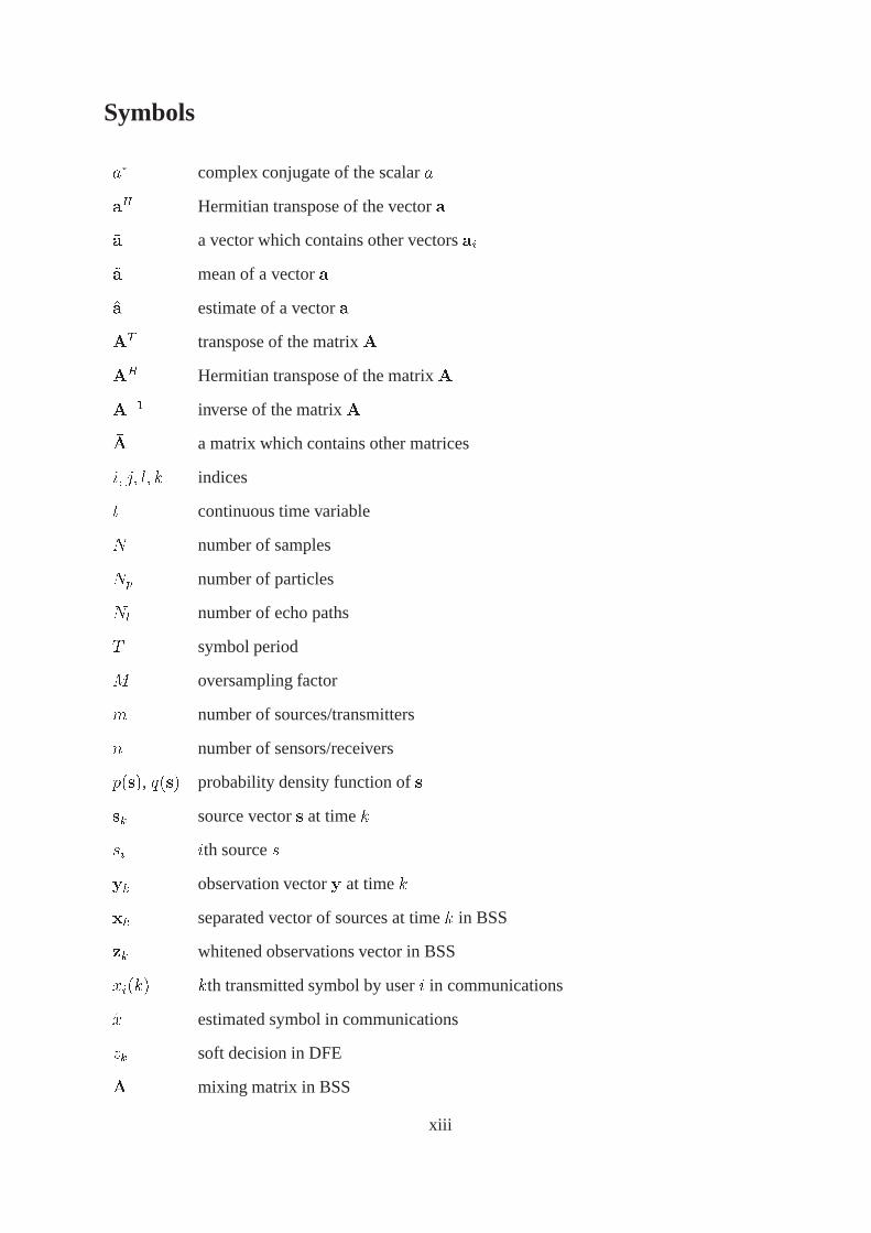
Symbols
�� complex conjugate of the scalar�
�� Hermitian transpose of the vector�
�� a vector which contains other vectors��
�� mean of a vector�
�� estimate of a vector�
�� transpose of the matrix�
�� Hermitian transpose of the matrix�
��� inverse of the matrix�
�� a matrix which contains other matrices
�� �� �� � indices
� continuous time variable
� number of samples
�� number of particles
�� number of echo paths
� symbol period
oversampling factor
number of sources/transmitters
� number of sensors/receivers
����, ��� probability density function of�
�� source vector� at time�
�� �th source�
�� observation vector� at time�
�� separated vector of sources at time� in BSS
�� whitened observations vector in BSS
����� �th transmitted symbol by user� in communications
�� estimated symbol in communications
�� soft decision in DFE
� mixing matrix in BSS
xiii

� separation matrix in BSS
�� orthogonal separation matrix in BSS
��� �th separation matrix at time� in blind deconvolution
� whitening matrix
� state transition matrix in state-space models
Kalman gain matrix
gain vector
� MIMO channel matrix
����� � �� prediction error covariance matrix
������ filtering error covariance matrix
� permutation matrix
� scaling matrix
� Kullback-Leibler divergence
identity matrix
� contrast function
�� orthogonal contrast function
����� entropies of the entries of��
� feedforward filter in DFE
� feedback filter in DFE
����� ���� non-linear functions
�� filter length for blind deconvolution
�� feedforward filter length
� feedback filter length
�� covariance matrix of�
� auto-correlation matrix
�� cross-correlation matrix
� cumulants
� matrix of correlation coefficients
�� kurtosis of the received�th source
xiv

���� score function
�� observation noise vector at time�
�� state noise vector at time�
� AR model order
� length of the channel
� matrix of eigenvectors
� diagonal matrix of eigenvalues
�� �th eigenvalue
�� �th eigenvector
Æ Kronecker delta
� delay used in decision feedback equalizer design
� delay
�� �� �� � adaptation step size parameters
��� channel coefficient from transmitter� to receiver�
� observation noise variance
� � expectation operator
�� � �� Euclidean norm
�� � ��� Frobenius norm
xv

xvi
Chapter 1
Introduction
1.1 Motivation
In blind source separation (BSS), multiple observations acquired by an array of sensors are pro-
cessed in order to recover the initial multiple source signals. The termblind refers to the fact
that there is no explicit information about the mixing process or about source signals. The con-
cept of blind source separation is related to independent component analysis (ICA). However,
ICA can be viewed as a general-purpose tool taking the place of principal component analysis
(PCA) which means it is applicable to a wide range of problems. Some application domains of
blind source separation are biomedical signal analysis, geophysical data processing, data mining,
wireless communications and sensor array processing.
Blind source separation techniques can be traced back to the work of Herault and Jutten [59]
in 1983 on a real-time algorithm used to solve the blind separation problem. In the related area of
blind channel equalization, Sato (1975) [115] and Godard (1980) [52] introduced techniques for
channel equalization using symbol statistics rather than known training symbol sequences. In the
years following the publication of these early works, the theory and practice of blind source sep-
aration have evolved tremendously. The instantaneous multiple-input multiple-output (I-MIMO)
noise-free linear model has been extended to linear FIR models and to nonlinear instantaneous
models. Many different algorithms have been proposed for BSS [1, 2]. These algorithms have
proven practical in varied areas of application. For instance, independent component analysis has
1
been used for separating contributions from different neural currents in the brain which appear as
mixed observations from an EEG array. There are, of course, many other applications. A search
of the IEEE publication database or other sources will reveal several thousand works related to
blind methods.
In recent years, the communications community has recognized the importance of blind sig-
nal processing techniques. This is partly due to the fact that wireless communications field ex-
perienced explosive growth, and demand for high data-rate services has been increasing. Blind
methods in communications use slightly different models from those used in blind source separa-
tion. For example, the distortion caused by multipath propagation in a communications channel
spreads the signal in time and causes frequency selective fading. The models used in communi-
cations are convolutive rather than instantaneous. Hence, for communications, the finite impulse
response multiple-input multiple-output (FIR-MIMO) model is appropriate. The termblind has
become quite popular for describing any estimation problem in which there is fairly limiteda
priori system information.
A good reason for investigating blind techniques in the context of communications is that
spectrum is a limited resource. Improved spectral efficiency and higher effective data rates are
important design goals of future communication systems. Use of multiple antennas at receivers
and/or at transmitters justifies MIMO models. Hence, blind techniques based on MIMO models
are very practical. Conventional techniques for receiver mitigation of communications channel
distortions require either knowledge of the channel parameter values or a sequence of known
training symbols. In particular, channel estimation and equalization rely on training signals.
This obviously decreases the effective data rate [126]. For time-invariant channels, the loss is
insignificant because only one training cycle is necessary. For time-varying channels, the training
has to be performed periodically, which significantly lowers the throughput. For example, in
GSM, about 20% of the symbols are used for training.
Most algorithms in communications systems are batch or block oriented and assume burst
transmission. Even if the channel is considered time-varying, during the burst period it is as-
sumed to be invariant. One limitation of batch blind equalization algorithms is their nonrecursive
structure, which effectively limits their applicability in time-varying scenarios requiring real-
2
time computation. In a slowly time-varying fading environment, blind algorithms could be used
to perform equalization. However, in the case of a deep fade, during which the equalizer may lose
track of the time-varying channel, batch algorithms may suffer. Structures that recursively com-
pute new symbol estimates by considering past channel and symbol estimates are better suited
for such time-varying channels [105].
Blind methods in communications are particularly appealing because they may allow all of
the symbol periods allocated for sending training symbols to be used for sending data symbols
instead. However, blind methods in communications have shortcomings. They may rely on unre-
alistic assumptions and they may also have poor convergence properties. Moreover, ambiguities
always remain when blind methods are used. Hence, so called semi-blind methods provide an in-
teresting alternative to both blind and non-blind methods. Optimal semi-blind techniques exploit
the same information as blind methods, and also use the information coming from the design of
the receiver [35]. By incorporating some known information, semi-blind techniques avoid the
problems encountered by blind methods. They may also allow shorter training sequences, so an
increase in the effective data rate can be obtained even if training sequences are not eliminated
entirely. The trade-off between blind and non-blind techniques makes the semi-blind methods
appealing for cost-effective and practical implementation in future receivers.
1.2 Scope of the thesis
The scope of this thesis is consideration of the problems of blind source separation, blind channel
equalization, and semi-blind channel equalization. The goal of the thesis is to define complete
algorithms capable of providing desired separation and equalization properties. The algorithms
should use as little prior information as possible for processing observations, while achieving
substantial performance improvements over existing techniques.
The main application area of the proposed algorithms is wireless communications. The de-
sign goal of the techniques is robust performance in noisy time-varying environments. Real-
time computation is an important issue in the face of time-varying systems. The computational
complexity of the resulting algorithms should be relatively low when compared to existing algo-
3
rithms. Simulation studies illustrating the performance of the algorithms should be performed in
a realistic manner.
1.3 Contributions of the thesis
The contributions of this thesis are in the area of blind source separation for I-MIMO and FIR-
MIMO models. Also the semi-blind FIR-MIMO equalization problem is considered in the case
of time-varying channels. The main application area considered is wireless communications.
However, simulations related to biomedical signal processing are also carried out.
The problem of on-line blind separation in the case of an instantaneous and slowly time-
varying linear mixing system is considered first. An algorithm is proposed based on a state-space
model. It employs subspace tracking and recursive estimation stemming from the Kalman filter.
It is demonstrated that separation of sources and noise attenuation can be performed simultane-
ously. Source signals are modeled using low order autoregressive models and noise is attenuated
by trading off between the model and the information provided by measurements. By using
a Kalman based source separation algorithm, the observation noise is taken into account. The
problems of detecting and adapting to changes that may occur in the mixing system are also ad-
dressed. Fractional sampling may be used to convert a FIR-MIMO model into a I-MIMO one
[143]. Using this technique it is shown that recursive BSS can be applied to equalization of
slowly time-varying channels. The performance of the separation algorithm is investigated in
simulations using biomedical and communications signals at different noise levels and using a
time-varying mixing system.
Recursive estimation is employed for tracking time-varying parameter values of communi-
cations channels. A semi-blind algorithm is proposed, with a short training sequence used at
the beginning of transmission to acquire the statistical information needed by the Kalman-based
channel estimation algorithm and also estimate the channel. After the training period ends the
algorithm relies on the decisions of an equalizer, and hence operates in a decision-directed mode.
The algorithm operates in two stages. In the first stage the channel is estimated and in the second
stage equalization is performed based on the channel estimates. Batch and on-line methods for
4
estimating the unknown noise statistics needed by Kalman filter are introduced. By including a
noise statistics estimation stage, less prior information is needed and improved performance is
achieved because critical parameter values are estimated rather than assumed. A multiple-input
multiple-output minimum mean square error decision feedback equalizer (MIMO MMSE-DFE)
is also derived. Simulations are carried out based on a realistic channel model [100].
The remainder of this thesis is organized as follows. Chapter 2 introduces the signal model
and the basic concepts employed in blind source separation. A brief review of the main classes
of algorithms is given and several applications are described. Chapter 3 contains a review of
adaptive whitening techniques. These methods are based on adaptive update of signal and noise
subspaces. The problem of tracking changes in the signal subspace is also considered.
In chapter 4, an adaptive blind source separation method is introduced. A review of adaptive
algorithms based on state-space model is given as well. The problem of modeling the sources or
the mixing matrix is also considered.
Chapter 5 deals with adaptive algorithms for semi-blind equalization. The chapter begins with
a brief introduction of the channel model that is used. The chapter focuses on algorithms which
perform joint channel estimation and symbol equalization. A description of the application of
Kalman filter to channel estimation and tracking is given and different derivations of the decision
feedback equalizer are presented. Finally, chapter 6 summarizes the results and contribution of
the thesis.
1.4 Summary of publications
The material in this thesis has appeared in seven other publications. Four relate specifically to
blind source separation and three relate specifically to semi-blind equalization.
In paperI, the problem of blind separation of signals in time-varying mixtures is addressed.
The proposed solution uses an adaptive whitening transform. A technique employing subspace
tracking is proposed. A Kalman filter based algorithm is used to perform recursive blind source
separation. The state transition matrix is augmented to contain a low-order autoregressive model
so as to have a more accurate prediction. Tracking changes in the signal subspace is another aim
5
of the paper. Examples using time-varying mixtures where the signal subspace changes in time
are presented with both test signals and communication signals.
Paper!! is an extension of the algorithm presented in paperI to solve the problem of separat-
ing both sub- and super-Gaussian densities. A fully adaptive algorithm is obtained by employing
a criterion for choosing a suitable zero-memory nonlinearity for each channel. In the simulation
examples, electrocardiogram (ECG) signals are employed in order to demonstrate a practical
application were signals with different kurtosis have to be separated and classical methods em-
ploying fixed nonlinearities for all channels fail. A slow variation of the elements of the mixing
matrix is also considered.
Paper!!!, shows the applicability of the recursive separation algorithm to the problem of
blind equalization. Based on a fractional sampling technique [143], the blind equalization prob-
lem is converted in a blind source separation (BSS)problem. Communication signals are consid-
ered in simulations and a slowly time-varying model is used for the mixing system.
Paper!" is one of the main publications of this thesis. A complete recursive algorithm for
blind source separation is presented. Simulation results are reported using both medical and
communications signals in different scenarios. Changes in the signal subspace are considered
and slowly time-varying mixing matrix is tracked.
Paper" deals with adaptive semi-blind equalization. The problem of multiple-input multiple-
output (MIMO) systems with application to communications is addressed. The time and fre-
quency selective nature of the channels is considered. A channel model based on measurements
is used in simulations. A state-space model is used to describe the system. The channel taps
are stacked in a state vector. A Kalman filter is employed to estimate and track the channel. A
minimum mean square error decision feedback equalizer for a system with two inputs and two
outputs is derived. The joint channel estimation/symbol equalization algorithm uses a training
sequence for initial parameter acquisition after that it runs in decision-directed mode. Results
presenting the mitigation of both the intersymbol interference (ISI) and inter-user interference
(IUI) are reported.
Paper" ! is another main publication of this thesis. Adaptive equalization of time-varying
MIMO channels is addressed. The results from paper" are extended to a general case. A
6
comprehensive derivation of MIMO minimum mean square error - decision feedback equalizer
(MMSE-DFE) is presented. Another goal is to design a channel estimator which does not require
too much information about the system other than knowledge of the training sequence. This
means that when using the state-space approach the state and measurement noise covariances
are estimated from the data. Both batch and recursive methods for estimating the noise covari-
ances are derived in the paper. Simulation results showing estimation of noise statistics, channel
tracking, and mitigation of ISI and IUI are reported.
Paper" !! addresses the problem of noise estimation in Kalman filter based MIMO equal-
ization. Estimating noise statistics is of great interest when using state-space models. Kalman
filtering requires accurate values of state and measurement noise covariances to work optimally.
In this paper a recursive method for estimating the noise statistics with application to equaliza-
tion of time-varying MIMO channels is proposed. The optimality of the estimates is tested using
non-parametric runs test on innovation sequences. The accurate estimation of noise covariance
matrices allows the Kalman filter to reliably estimate the state, thus leading to improved equal-
ization performance.
All of the simulation software for the all of the original papers of this dissertation was written
solely by the author, with the exception of that used for papers!" -" !!, which had contributions
from the other authors. The original Kalman-filter-based separation algorithm which appeared in
paper!" was the idea of the first author. The author of this thesis contributed material relating to
subspace tracking, detection of changes in mixing system and selection of appropriate nonlinear-
ities leading to a more complex recursive algorithm which is described in papers!-!" . He was
mainly responsible of planning experiments for all the papers. The author derived the analytical
results in paper" ! and did most of the writing of papers!-!!!, and" -" !!. The co-authors
collaborated in experiment design, provided guidance for the author’s proofs, and contributed to
the writing of the final version of each paper.
7

8

Chapter 2
BSS model
There is plenty of recent work on blind source separation (BSS) in the signal processing, com-
munications and neural network research communities. Recent publications include article col-
lections [44, 56], special magazine issues [1, 2], monographs [51, 86] and two comprehensive
books [28, 65]. Some review articles do exist [79] and also many articles have been published
[16, 17, 20, 30, 68, 71, 75, 103].
This chapter introduces different models used in blind separation and the underlying assump-
tions that justify their use. Several categories of algorithms are presented and key concepts are
described. The problem of blind deconvolution and a few important applications of blind sepa-
ration are also discussed in brief.
2.1 Problem formulation and assumptions
The goal of blind source separation is to recover original source signals from sensor observations
that are mixtures of the original source signals. Over the years, several models [31] of the mixing
process have been used. We start from the basic linear model that relates the unobservable source
signals and the observed mixtures:
�� � ���� (2.1)
where� is an� � matrix of unknown mixing coefficients,� � , � is a column vector of
source signals,� is a column vector of� mixtures, and� is the time index. This model is
9
instantaneous because the mixing matrix contains fixed elements, and alsonoise-free. If noise is
included in the model, it can be treated as an additional source signal or as measurement noise.
In the case when it is present as measurement noise, the model becomes:
�� � ��� � ��� (2.2)
where the noise vector�� is of dimension� � �. The mixing matrix may be constant, or can
vary with the time index�. In the time-varying case,� becomes��. In multichannel blind
deconvolution or blind equalization, the�-dimensional vector of received signals�� is assumed
to be produced from the-dimensional vector of source signals using the�-domain mixture
model:
���� � ��������# (2.3)
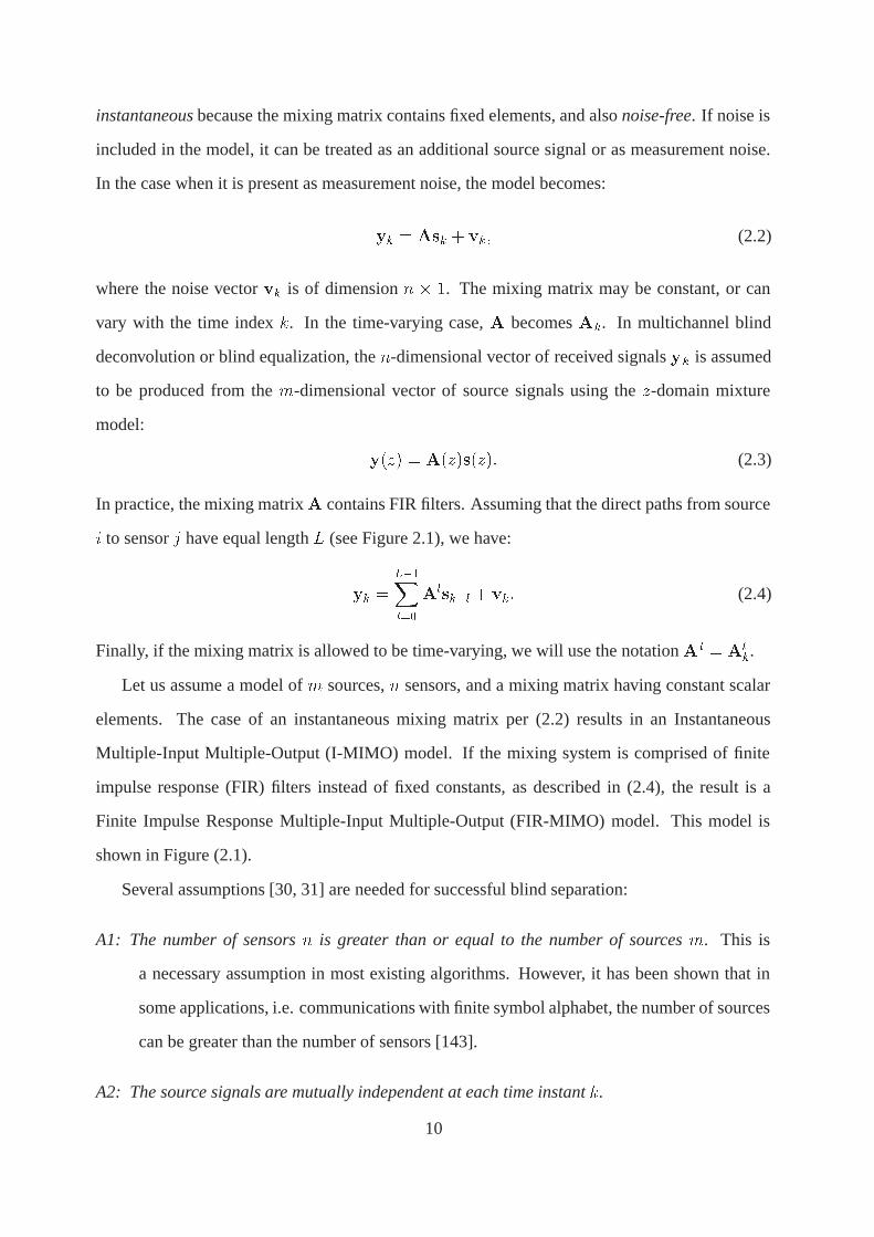
In practice, the mixing matrix� contains FIR filters. Assuming that the direct paths from source
� to sensor� have equal length� (see Figure 2.1), we have:
�� ��������
������ � ��# (2.4)
Finally, if the mixing matrix is allowed to be time-varying, we will use the notation� � � ���.
Let us assume a model of sources,� sensors, and a mixing matrix having constant scalar
elements. The case of an instantaneous mixing matrix per (2.2) results in an Instantaneous
Multiple-Input Multiple-Output (I-MIMO) model. If the mixing system is comprised of finite
impulse response (FIR) filters instead of fixed constants, as described in (2.4), the result is a
Finite Impulse Response Multiple-Input Multiple-Output (FIR-MIMO) model. This model is
shown in Figure (2.1).
Several assumptions [30, 31] are needed for successful blind separation:
A1: The number of sensors � is greater than or equal to the number of sources . This is
a necessary assumption in most existing algorithms. However, it has been shown that in
some applications, i.e. communications with finite symbol alphabet, the number of sources
can be greater than the number of sensors [143].
A2: The source signals are mutually independent at each time instant �.
10
A3: At most one source is normally distributed. This a valid assumption only for the noise free
model (2.1).
A4: The mixing matrix � is full rank. If the mixing matrix is comprised of FIR filters, which
is the case of FIR-MIMO systems, then it admits an FIR left inverse, i.e. it is minimum
phase.
A5: Sources have finite second moments.
In recent years, new methods and new underlying assumptions have been introduced. Among
the previously mentioned assumptions, some of the hypotheses are application dependent.
A6: Sources are zero mean and stationary.
A7: A part of the sources are known at the receiver. This hypothesis is used in communications
in the form of atraining sequence.
A8: Sources have constant modulus. This property arises in the case of -ary phase shift keying
(M-PSK) sources.
A9: Sources have finite alphabet. This means that the source signals are chosen from a finite set
such as� BPSK or a set of phase shifts for DQPSK signal.
A10: The noise � is white and Gaussian.
v1
vj
vn
y
y
yn
1
ji
1
m
11
1j
ij
mj
mn
a
a
a
a
a
s
s
s
Figure 2.1: FIR-MIMO model.
11
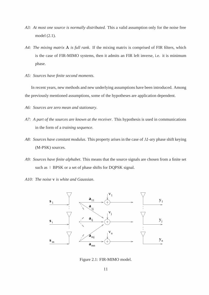
The separation task at hand is to estimate the original source signals with high fidelity given
noisy mixture measurements. In the case of I-MIMO model this is done by estimating either a
separating matrix� or a mixing matrix ��. An estimate� of unknown sources� is then given
by
��� � �� � ��� � ������# (2.5)
Some algorithms include a whitening stage prior to separation. During this stage the observed
mixtures are spatially decorrelated and signal powers are normalized to unity. In addition, by
projecting the input data along signal subspace eigenvectors, the problem becomes easier to
solve because the separating matrix will be an orthogonal matrix. Reducing the dimension of data
from � to is very important in some applications were� is much greater than. For example,
in the case of medical EEG and MEG measurements, this is often necessary because of the high
dimensionality of the data. If the observations have been whitened, no inversion is needed to
separate the sources since the separating matrix is orthogonal with���� � ��� . The sources may
be recovered to within a permutation and a scaling, by matrices� and� respectively:
�� ���# (2.6)
The product�� may be seen as a performance measure. Then a perfect separation leads to an
identity matrix,�� � .
s
v
y xk
k
kk Ak W
Figure 2.2: Adaptive I-MIMO model.
Source separation is a filtering problem that includes separation, deconvolution, or equal-
ization [31]. Estimation of the mixing matrix���, in the case of FIR-MIMO, is also known as
channel identification. Whena priori information such as training sequences is available, the
process of source separation or channel identification is said to beinformed. When no infor-
mation about the sources or channel is known, such as a known training sequence of sufficient
12
length, the process of recovering the transmitted information or to identify the channel is said to
beblind. If only limited knowledge about the sources is present, for example if the signal values
are known part of the time, the processing is calledsemi-blind [31].
2.2 Key concepts in BSS
The main assumption of ICA is that the source signals� are independent. The initial sources
together generate an-dimensional probability density function (pdf) ����. Statistical indepen-
dence among the sources means that the joint source density factorises as:
���� ������
��������# (2.7)
The same statement can be done for the separated sources�. If the pdf of the estimated sources
also factorises then they are independent.
The Kullback-Leibler divergence is a measure of the distortion between two probability den-
sity functions����� and ����. The Kullback-Leibler divergence between����� and ���� is
given by:
���� � ��
����� ��
������
����
�$�# (2.8)
This expression can be interpreted as a distance measure because it is always non-negative and is
equal to zero only when����� � ����. Due to this property, Kullback-Leibler divergence can
be used to measure the mutual independence of output signals�.
Estimation of a source model in blind separation usually involves formulating and then min-
imizing a contrast function [30]. Due to the fact that in practice finite data sets are available, the
concept of the estimating function was introduced. These concepts will be briefly described in
the next sections.
2.2.1 Contrast functions
Source separation can be obtained by optimizing a contrast function. These are real-valued func-
tions of the distribution of the output�� � ��� and which must be designed such that separation
is achieved when they reach their minimum value. In other words, using a contrast function turns
13

the source separation problem into an optimization problem. Typical optimization algorithms
include gradient methods, Newton-type methods, and other techniques [65].
Contrast functions are based on entropy, mutual independence, higher-order decorrelations,
or divergence between the joint distribution of� and a model. Important properties of the al-
gorithms used to optimize the contrast functions include convergence speed, numerical stability,
and memory requirements.
Likelihood
Let � denote a random vector with distribution . The maximum likelihood principle is associated
with a contrast function:
������� � ����� ���# (2.9)
This means that we have to find a mixing matrix� such that the distribution of the separated
sources� is as close as possible (in the Kullback divergence sense) to the hypothesized distribu-
tion of the original sources. One problem of ML contrasts is that if the hypothesized distributions
of the sources are not correct we will not obtain the desired results. Obviously, in blind separation
the source distributions are unknown.
Mutual Information
In the case of mutual information, the idea is to minimize����� ��� with respect to� taking
into account the distribution of� and with respect to the model distribution�. Let �� denote a
random vector with independent entries and with each entry distributed in the same way as the
corresponding entry of�. We obtain:
����� ��� � ����� ���� ������� ���# (2.10)
The last term is minimized by taking� � �� for which������ ��� � �. The contrast function is:
������� � ����� ���� (2.11)
which can be interpreted as the Kullback divergence between a distribution and the closest dis-
tribution with independent entries.
14
Orthogonal contrasts
These contrasts are used when the data has been prewhitened. In such cases, the minimization
of the contrast function must take place under the constraint that������� , where� � is the
expectation operation. The mutual information contrast function becomes:
�������� ���
� �� � (2.12)
where� � is the entropy. In other words, minimizing the mutual information between the entries
of � is equivalent to minimizing the sum of the entropies of the entries of�.
Cumulants
Higher Order Statistics (HOS) can be used to define contrast functions. Higher order information
may be expressed by cumulants. Given the zero-mean vector�, the most relevant cumulants for
BSS are those of second and fourth order [21], defined as:
��� ��def� � ��� �� (2.13)
and as:
����� ��def� � ��� ��� ��� ��� � ��� �� � ��� ��� (2.14)
� ��� �� � ��� ��� � ��� �� � ��� �� #
The third order cumulants are:
���� ��def� � ��� ��� �� # (2.15)
Under the assumption of independence, the cross entries of the sources are zero, and:
��� �� � ������ def� �
� � (2.16)
where �� is the variance of the�th source. Similarly,
����� �� � ������� ��
������ def
� ��� (2.17)
15
where�� is the kurtosis of the�th source. Signals with positive kurtosis, (the tails of their densities
decay more slowly than the Gaussian density and are sharply peaked around their mean) are
known as super-Gaussian. Signals with negative kurtosis (rapidly decaying tails) are called sub-
Gaussian.
The likelihood contrast��� is a measure of mismatch between an output distribution and
a model source distribution. A cruder measure can be defined from the quadratic mismatch
between the cumulants:
�� ���� ����
���� ����� ��� ������ ����
���� ����� �
� ����
(2.18)
and
�� ���� ������
������ ����� ����� ������ ������
������ ����� �������� � (2.19)
whereÆ is the Kronecker symbol. Cardoso [21] pointed out that the measure defined by (2.18) is
not a true contrast in the BSS sense, as it reaches zero when� is linearly decorrelated. The use
of the fourth order information�� leads to independence.
If � and� are symmetrically distributed with distributions that are close to normal, then the
maximum likelihood approach can be approximated as [21]:
��� � � ���� ��� � ������� (2.20)
def�
�
����������� � �� ����� #
If the kurtosis values of all sources have the same sign, the sum of the fourth moments can be
used as a contrast function [94]:
��moreau����def�
�����
������# (2.21)
Cardoso proposed to test the independence on a smaller subset of cross-cumulants [24]. His
approach resulted in the Joint Approximate Diagonalization of Eigen-matrices (JADE) technique,
which, under the whiteness constraint, has the contrast function:
������def�
����� ������
������ ���� # (2.22)
16
2.2.2 Score functions
Choosing thescore or squashing functions is very important since they describe the source model.
The score functions��, # # # , �� are defined as the log derivatives of the source densities �, # # # ,
�:
�� � � � �� ��� or � ��� � � � ����
� ��� # (2.23)
In the case of a zero-mean unit-variance Gaussian variable� with density ��� � ��%�����
���� ���&��, the associated score function is� ��� � �. Gaussian densities are associated with
linear score functions. Non-Gaussian modeling results in considering non-linear score functions
[21].
Several approximations for the score functions have been used in the literature. For example,
Bell and Sejnowski [17] used a fixed source model assuming that all the initial sources have
the same kurtosis. This type of processing was further developed by Girolami [49], who used
different score functions for sub- and super-Gaussian sources in order to separate mixtures of
densities. Based on the stability analysis introduced in [8], Douglas [39] proposed switching
between nonlinearities by analyzing the statistics on each output channel. Other approaches do
exist for selecting the score functions [78]. Generalized exponentials or mixtures of Gaussians
have also been used to model sources. See [112] for a review and [90] for a more detailed
analysis.
2.2.3 Estimating functions
Due to their design, all contrast functions reach their minimum at a separating point. However, in
practice contrast functions are estimated from a finite data set. Thus, the sample-based contrasts
depend on the sample distribution of�. Due to the errors introduced by estimation using a small
data set, statistical characterization of the minima of sample-based contrasts is needed. In this
sense the notion of an estimation function was introduced [21]. The estimation function for blind
separation is a function � �� ���� . Considering a batch of� samples, the estimation
function is associated with an estimating equation:
�
�
�����
���� � �# (2.24)
17
The gradient of the ML contrast function was found by Pham [107]:
���� ���� � � � ��� � (2.25)
where
� ��� def� � ����� � (2.26)
and is an identity matrix. The ML contrast function achieves its minimum at points where its
relative gradient cancels, i.e. at the points which are solutions of the equation� � ��� � �.
We note that ML estimates correspond exactly to the solution of an estimating equation [21].
Under the whiteness constraint, the ML estimation function is:
�� ��� def� ��� � � � ����� � �� ���� # (2.27)
The estimating function for the orthogonal contrast��moreau���� given in (2.21) has the same form
as given in (2.27) but with�� ���� � ��� . Not all the contrast functions have estimating functions
which can be expressed in the form (2.24). However, one can often find an asymptotic estimating
function in the sense that the solution of the associated estimating equation
is very close to the minimizer of the estimated contrast [21].
2.3 Different classes of algorithms
The ways in which separation algorithms process the data can be used as basic classification
criteria. There are situations when the whole data set is available. In such case the processing
is done in batch mode [24, 63, 64] considering the whole set of available samples. Algorithms
of this type arebatch algorithms. In real-time applications the data is available one at the time,
meaning that at each time index� we receive a�-dimensional vector of observations��. Based
on the new received data vector and possibly on a vector of some previously-received data, the
task is to estimate the initial sources. Algorithms of this type areon-line algorithms [23].
The advantage of on-line algorithms is that they enable faster adaptation in a time-varying
environment due to the fact that the input�� can be used in the algorithm immediately. A
resulting trade-off is that the convergence may be slow and the convergence rate may depend on
the choice of the learning rate. A bad choice of the learning rate can lead to very poor results.
18
Batch algorithms should be used in situations where fast real-time adaptation is not necessary
[64] and in which mixing systems or source statistics are not time-varying.
Existing blind separation algorithms can be divided into two main groups. Methods in the
first group attempt to find a separation matrix directly, while the methods from the second group
use whitening before determining a separation matrix. Whitening has some advantages such as
reduction of the data dimension from� to and also noise attenuation. The separation task
is made easier because the components of the whitened vectors� are already uncorrelated and
we have to search for an orthogonal separating matrix. Moreover, using real-world data it has
been shown [48] that whitening can improve both the convergence speed and the separation
performance. A good example is the application of BSS to anti-personnel land mine detection
[77]. In this case, blind separation is used to detect the anti-personnel land mines based on a
set of sensor signal measurements. The number of mixtures is very high in comparison with
the number of sources, i.e. there may be� � ���� mixtures and � �� sources. Thus, it is
impractical to apply algorithms which search for a separation (or mixing) matrix without prior
whitening of the sources. Whitening has also some disadvantages. For example, if some of the
source signals are very weak or the mixture matrix is ill-conditioned, prewhitening may greatly
reduce the accuracy of the algorithm.
Different techniques for recovering the transmitted sources have been proposed. One of the
first algorithms that appeared in the literature was proposed by Herault and Jutten [58]. The
algorithm is based on the idea of measuring independence of the separated sources by pairwise
nonlinear decorrelation. The mixing model of equation (2.1) is used. If the sources are zero
mean and have symmetric densities, and if the selected nonlinearities� and� are odd, then the
expectation����������� is zero.
The family of gradient-based algorithms is very important in the BSS literature. Bell and Se-
jnowski [17] derived an algorithm based on maximizing the entropy of a nonlinear output. The
algorithm uses a stochastic gradient optimization method without prewhitening, and successfully
separates speech sources. Amari et al. [10] proposed an improvement to Bell’s stochastic gradi-
ent algorithm, based on using the natural gradient. The goal is to update a separation matrix in
the direction of the natural gradient [7], which leads to faster convergence than with stochastic
19
gradient algorithms. A similar algorithm, called relative gradient, was independently proposed
by Cardoso and Laheld [23]. This algorithm has also the equivariance property, meaning that its
behavior does not depend on the nature of the mixing matrix. Amari proposed a similar algorithm
based on minimizing the mutual information using natural gradient learning [10].
Another class of algorithms used to optimize contrast functions is represented by Jacobi al-
gorithms. They are called Jacobi due to the fact that the goal is to maximize measures of in-
dependence by a technique akin to that of the Jacobi method of diagonalization. The Jacobi
method is an iterative technique of optimization over the set of orthonormal matrices which are
obtained as a sequence of plane rotations. Several algorithms have been proposed. The first one
was introduced by Comon [30]. As pointed out in [22], this is a data-based algorithm, meaning
that it works through a sequence of Jacobi sweeps on whitened data until a given contrast is
optimized. A statistic-based algorithm, JADE, was introduced by Cardoso [24] where the plane
rotations are applied to the cumulant matrices, instead of to the data itself. A mixed approach,
called SHIBBS (SHIfted Blocks for Blind Separation), was introduced in [22] where the update
to get the separated sources is made on the data itself and the rotation matrix that is applied to the
data is computed in a statistic-based procedure. One advantage of Jacobi algorithms is that no
tuning is needed (in their basic versions) as opposed to the gradient-based algorithms in which a
learning schedule is necessary and usually implemented in a heuristic manner [22].
Stemming from Principal Component Analysis, the class of nonlinear PCA algorithms is also
of great importance [73]. Several algorithms were introduced, for instance that of [72]. It has
been shown that nonlinear PCA can separate signals in the presence of a noisy time-varying
mixing model [74, 75]. The connections between several ICA algorithms, such as the Bell-
Sejnowski [17] algorithm or the EASI algorithm[23], and information-theoretic contrasts have
been shown by Karhunen et al. [76]. An overview of adaptive algorithms is given by Amari et
al. [9], and a detailed description of statistical principles used in BSS is made by Cardoso [21].
20
2.4 Blind Deconvolution
Plenty of research has been done in the area of blind deconvolution [9, 12, 54, 57]. Various
scenarios have been considered, starting from the single-input multiple-output (SIMO) model
obtained by oversampling at the receiver or by using several receivers [62], to the MIMO case
[12, 54]. Different techniques based on Higher Order Statistics [131], subspace decomposition
[89] or multichannel frequency-domain deconvolution [84] have been reported in the literature.
Typically assumptions include linear time-invariant (LTI) systems, infinite SNR, and infinite
equalizer length [131]. In contrast, real systems are time-varying (TV), SNR values are low,
and equalizer lengths are finite.
Using the model described by equation (2.4), the goal of blind deconvolution is to estimate
source signals using a multichannel linear filter of the form:
�� �������
�������� (2.28)
where��� are the� � �� matrix coefficients of the separation system and�� is a filter length
parameter.
A very interesting technique for possibly transforming the BSS algorithms into multichannel
blind deconvolution algorithms is presented in [38, 40]. This is based on assuming that � �
and that the mixing matrix� is circulant. A circulant matrix is completely specified by any one
row or column, as the other rows or columns of the matrix are simply modulo-shifted versions
of this row [38]. For example, the first column of� is �� �� # # # ����� , the second column of
� is ���� �� # # # ����� , and so on. However, a principal problem is that the assumption of a
circulant matrix is artificial. No physical mixing system exhibits this structure [38].
The presentation of blind deconvolution techniques based on this transformation is beyond the
scope of this discussion. We will simply state that the transformation process involves following
three rules that make associations between matrices in the BSS task, such as�, �� and matrix
sequences in the multichannel blind deconvolution task such as� �, ���. These three rules can
be summarized as follows [38, 40]:
� Multiplication of two matrices in instantaneous BSS (I-BSS) is equivalent to convolution
of their associated matrix sequences in multichannel blind deconvolution (MBD).
21
� Addition of two matrices in I-BSS is equivalent to element by element addition of their
associated matrix sequences in MBD.
� Transposition of a matrix in I-BSS is equivalent to element by element transposition and
time reversal of its associated matrix sequence in MBD.
The previous procedure can be applied to the density matching BSS algorithm using natural
gradient adaptation [12, 38] and to contrast function optimization for I-BSS algorithms.
2.5 Applications of BSS
Due to the volume of research on blind separation over the past years, the recognized applications
of BSS are numerous. For example, inbrain imaging applications we may capture recordings
of electric (electroencephalograms, EEG) and magnetic (magnetoencephalograms, MEG) fields
of signals emerging from neural currents within the brain. It is important to extract the essential
features from the data allowing a better representation and understanding of their properties. An
important application of BSS is the separation of artifacts from EEG and MEG data [133].
In wireless communications an essential issue is the sharing of the common transmission
medium among several users. In Code Division Multiple Access (CDMA) systems all users oc-
cupy the same frequency band simultaneously. The users are identified via unique codes. During
the transmission different users’ signals become mixed, the user can be identified from the mix-
ture by applying the code at the receiver. In downlink (mobile phone) signal processing each user
knows only one code. The codes of the other users are unknown. By modeling the CDMA signal
as a linear combination of convolved independent symbol sequences [33], BSS techniques can
be applied for the separation of the sources. I-MIMO model is used for narrowband communi-
cations applications and FIR-MIMO for frequency selective channels. Another communications
application can be in GSM where blind separation can be used to achieve blind equalization
under some conditions [144].
Speech separation is an important and attractive application domain for BSS. One of the main
applications is the separation of simultaneous audio sources in reverberating or echoing environ-
ments, i.e. inside a room. Speech enhancement is a very desirable application where only one
22
signal is of interest and the rest are considered to be nuisance signals [50]. Enhancement of voice
quality in mobile phones, would be one important application, especially in car environments.
In real environments multiple paths are common and blind deconvolution is usually necessary.
Torkkola [127] gives an extensive survey, with many references, of blind separation of audio
signals.
Many other applications exist [65]. In fact, every application which leads to the BSS model
can be of interest even if the assumptions about the BSS model are not so close. In many practical
BSS applications, observations are noisy, the mixing system and/or source statistics may be time-
varying, and source signals may appear and disappear randomly. Moreover, the delays associated
with batch processing may be intolerable. Hence, it is important to develop recursive separation
algorithms that take into account both noise and the time-varying nature of the problem and that
allow real-time computation.
23

24
Chapter 3
Adaptive Whitening
3.1 Introduction
Several BSS algorithms usewhitening transform prior to performing separation. Due to this
operation, the search for a separating matrix is reduced to the search for an orthogonal separating
matrix. The number of unknown parameters which must be determined is reduced as well. By
definition,�� is a whitening matrix if the outputs�� � ���� are spatially white, i.e.�����
��
��
�� � . Adaptive whitening consists of updating the matrix�� such that it converges to a point
where�� � . The covariance matrix�� may be time-varying if the mixing matrix and/or
the sources are time-varying. The ability to adapt is needed if�� varies, otherwise, a recursive
formula has only computational advantages. Let us consider the noisy model from (2.2). When
the number of sensors� is greater than the number of sources, the covariance matrix�� is
given by:
�� � ����� � �
� (3.1)
where�� � ������
and � is the noise variance. Using matrices of eigenvectors and eigenval-
ues,�� can be written as:
�� � ������� ������
�� � (3.2)
where�� is an � diagonal matrix given by�� � diag��� # # # � ��, with �� denoting
theth largest eigenvalues of the covariance matrix��, �� is an� � matrix containing
the �� principal eigenvectors,�� � ��� # # # � �� corresponding to the largest eigenvalues.
25
The subspace spanned by the eigenvectors contained in�� is the signal subspace. The matrix
� � diag����� # # # � �� is diagonal and contains the remaining� � noise eigenvalues and
�� � ����� # # # � �� contains the corresponding�� noise eigenvectors. The subspace spanned
by the noise eigenvectors is the noise subspace. The signal subspace is orthogonal to the noise
subspace.
The dimension of the signal subspace can be estimated by inspecting the eigenvalues of��.
The signal subspace eigenvalues usually exhibit a clear pattern. They are a linear combination
of the source powers� ������ added the noise power �
[73]. If the signal to noise ratio (SNR)
is high enough, the largest eigenvalues are much larger than the other�� eigenvalues. At
low SNR this pattern may not be so clear, and information theoretical criteria such as minimum
description length (MDL) can be used to find the number of signals [134].
The chapter presents adaptive methods for performing whitening. The techniques addressed
are based on Principal Component Analysis. Serial update of whitening matrices is also pre-
sented. We also discuss how changes in the dimension of the signal subspace can be tracked in
real time.
3.2 Subspace Tracking
Since whitening is essentially a decorrelation followed by scaling, Principal Component Analysis
(PCA) can be used [65]. Considering the covariance matrix�� � ���� , where� is a� � �
matrix of eigenvectors and� is a�� � diagonal matrix of eigenvalues, the whitening matrix�
is given by:
� � ������� # (3.3)
If more sensors than sources are present in the system, the whitening matrix is formed using the
signal subspace. Thus�� � ������ ��� . This reduces the dimension of the data from� to and
allows the search for an orthogonal separating matrix of dimension�. The whitening matrix
� introduced in (3.3) is not a unique whitening matrix. Let consider� an orthogonal matrix and
26
let apply the transform�� to the received data��. Then, we obtain:
�����
��
�� ���
����
��
�����
� ��������������������
� � �� � � (3.4)
where we have used the orthogonality of the eigenvectors, i.e.��� �� � � for � � �. Thus, any
matrix��, with� an orthogonal matrix, is also a whitening matrix.
If the covariance matrix of the received data varies in time, on-line update of the eigenvalues
�� and eigenvectors�� is needed in order to accurately track/adjust the whitening matrix�� at
each time step�. A good review of methods for tracking principal singular values and vectors is
given by Comon and Golub [32].
Any subspace tracking algorithm which exhibits good convergence and tracking capability
can be used for adaptive whitening. Some subspace tracking algorithms track only the eigenvec-
tors. Using these results in decorrelated data with a possibly-incorrect scale. One BSS algorithm
that performs only decorrelation and then employs a contrast based approach to find a separation
matrix was introduced by Douglas [36]. However, some of the BSS algorithms require that the
data has unit power. Thus an estimate of the eigenvalues is also needed in order to update the
whitening matrix��.
3.2.1 PAST and PASTd
Yang [136] proposed an on-line algorithm for tracking the-dimensional principal signal sub-
space by using an approximate Recursive Least Squares (RLS) type of update. The Projection
Aproximation Subspace Tracking (PAST) algorithm computes a subspace eigenvector matrix
estimate�� that minimizes the least squares criterion:
����� ��� ������
���� � �� � ���� ��� (3.5)
where� � � denotes the Euclidean norm and� is a forgetting factor needed in tracking time-
varying system. For notational convenience we will use� instead of�� in the following. It is
also assumed that we have more sensors than sources, i.e.� ' . The recursive update for the
27
�� matrix� at time� is:
�� � �������
�� � �� � ������
� �������
� � ���������
�� ��
�Tri���� � ��
���
����
�� � ���� � ��
�� � (3.6)
where�� is the� � � a priori estimation error vector (or the innovation),� is the � � gain
vector and�� is the � inverse of the correlation matrix��. The notation Tri means that
only the upper triangular part of the argument is computed. Its transpose is copied to the lower
triangular part so that the resulting matrix becomes symmetric.
The forgetting factor� ( � � � allows tracking when the system operates in a non-stationary
environment. The value� � � corresponds to the standard least square solution. The choice
of initial values for� and� affects the transient behavior but not the steady state performance
of the algorithm [136]. In order to avoid transient behavior problems���� must be a Hermitian
positive definite matrix and���� should contain orthonormal vectors. These matrices can be
calculated, for example, from an initial block of data.
The PAST algorithm does not maintain the orthonormality of the estimate�� during the
adaptation [136]. Douglas proposed [37] a modification of PAST that enforces the constraint
����� � . This algorithm employs identical Householder transformations to update��. For
adaptive subspace analysis, the general Householder-based update is:
�� � ����
� � ���
��
��� ��� (3.7)
where���� is a matrix whos columns have to be rotated and�� is the Householder vector.
The Householder-based update for�� behaves similarly to PAST within the constraint space
����� � . The modifications are as follows:
�� � �� � �
�� �� �� �����
�� � ���� ���
��
� � ��� �� ��� � �� �
28
where��, � and�� are computed as given in (3.6).
Based on the deflation technique, Yang [136] introduced PASTd algorithm derived from
PAST. PASTd enables also the sequential estimation of the eigencomponents. The key idea
in this technique is the following. First the most dominant eigenvector is updated by applying
PAST algorithm with � �. Then, the projection of the current data vector�� along this eigen-
vector is removed from the current data vector. At this stage, the second dominant eigenvector
becomes the most dominant eigenvector and can be extracted in the same manner. Repeating
this procedure, all desired eigencomponents are estimated sequentially. The algorithm may be
summarized as follows:
��� � ��
for � � �� �� # # # �
��� �������
�����
)�� � �)���� � ������
��� � ��� � ��������
��� � ����� � ���
������
�
)��
������ � ��� � ����
��� (3.8)
where��� is an estimate of the�th eigenvector of�� and)�� is an exponentially weighted esti-
mate of the corresponding eigenvalue. The drawbacks of PASTd are the fact that it loses the
orthonormality between�� and a slightly increased complexity if�� .
3.2.2 Subspace tracking by subspace averaging
Karasalo [70] proposed an algorithm for updating the covariance matrix by signal subspace av-
eraging. A similar method was also proposed by Tufts et. al. [130]. The algorithm operates as
follows [70]. The received data vector�� is split into signal and noise subspaces:
�� � ������ � ��*�� (3.9)
29
where������ define the old signal subspace,�� is part in orthogonal subspace and* is a nor-
malization scalar. This decomposition involves computing the following variables:
�� � ������� (3.10)
�� � �� � ������ (3.11)
*� � � �� ���� � ��&*�# (3.12)
A major computational advantage stems from constructing a smaller����� ���� matrix�
which preserves the properties of the��� covariance matrix�� and contains all the information
needed to compute both the squared singular values�� and the associated eigenvectors��.
� �
� �
������ ������
���� ���
���*�
�� � (3.13)
where���� is a diagonal matrix containing the square roots of the principal eigenvalues
estimated at time step���, ��� is the square root of the noise variance,�� and�� are weighting
coefficients. A singular value decomposition (SVD) of the matrix� must be performed:
���� � �# (3.14)
Finally, eigenvector and eigenvalue estimates are updated. The square roots of the eigenvalues,
��, are found in the upper left corner in�. The corresponding eigenvectors are the first
columns in:
���� ���# (3.15)
An update of the noise variance � is also obtained:
�� �
�
��
� ���� � ���� ����
����
�� (3.16)
where ���� is the � � diagonal element of�. The weight coefficients�� and�� are very
important in the process of tracking the principal subspace. The better the estimates of these
coefficients, the closer the covariance matrix��� is to the local true covariance matrix��. In
[70], the update of the weight coefficients�� and�� is done in such a way that the algorithm
initially relies on the observed data and later relies more on the computed eigen-decomposition
than on new received data.
30
One may be also interested in an update of the complete covariance matrix. It is obtained as
follows:
��� � ��� ������� � � �
� # (3.17)
where the estimates���, ��� and� �� are found using the previous algorithm. The computational
complexity of the previous algorithm is relatively low. However, one SVD is involved in the up-
date process. The dimension depends on the dimension of the signal subspace. Hence, substantial
savings are obtained if the dimension of signal subspace is small compared to the dimension of
the data covariance matrix.
3.2.3 Serial update of the whitening matrix
Another method for adaptive whitening was proposed by Cardoso. In [23] the serial update of the
whitening matrix is based on minimizing the ’distance’ between�� and . The Kullback-Leibler
divergence between two normal distributions with covariance matrices�� and is:
����� ��
����*+ ����� �� ��� ����� # (3.18)
A whitening matrix is obtained when����� � �. This can be achieved by using the following
update rule [23]:
���� � �� � ,�����
�� �
���� (3.19)
where,� is a variable adaptation step size.
3.3 Tracking changes in signal subspace
An important issue in adaptive subspace tracking algorithms is the ability to track possible
changes in the dimension of the signal subspace. Eigenvalue inspection of�����
�solves the
problem of identifying the dimension in the case when�� is time invariant. However, in adaptive
PCA the problem becomes more challenging since at each time� we receive a new observation
vector��. Thus, assuming that we know the number of principal eigenvalues at time step� � �
and based on the new information vector received at time�, we must decide if the number of
sources has changed or remained the same.
31
A solution to this problem was proposed by Real et. al. [111]. They first consider the
observation matrix�� � ����� � # # # ��� given by a window of length��. As a new information
vector�� becomes available, the energy�� of the matrix�� is computed as the square of the
Frobenius norm:
� �� ����� ���� ��� � � ����� ��� � � �� ��� # (3.20)
From the matrix energy�� we subtract successively larger sums of squares of the largest
of the estimated eigenvalues�� until the difference lies below a chosen threshold value. For
� � �� # # # � we compute:
�� � �� ������
��� (3.21)
and each value of�� (including��) is compared to the threshold. The number of times�� exceeds
the threshold is the estimated dimension of the signal subspace. However, some problems still
arise from the selection of the threshold value. This can be set either theoretically from knowl-
edge or assumption about the power in the orthogonal subspace or heuristically from estimates
of that power [111].
In blind source separation it is also of great interest to detect changes in the mixing system.
Paper!" proposed computing a sample covariance matrix in a relatively small processing sliding
window and comparing the matrix to the covariance matrix constructed by the subspace tracker
(3.17). The sample covariance matrix at time� in a window of� samples may be recursively
computed by:
�� � ���� ��
����
�� �
�
������
���� # (3.22)
A matrix of correlation coefficients is formed from the covariance matrices��� and ���. The
following dimensionless expression� ��� � ��� ��� ��� ��
(3.23)
is compared to a threshold value. If the value of (3.23) exceeds the threshold, the weighting used
in the subspace tracking is reset to the initial weights so that recent measurements are weighted
more heavily.
Whitening is an important stage for one class of separation algorithms. Hence, accurate
values resulting from eigendecomposition are needed in order to obtain robust whitening. In
32

time-varying scenarios it is important to track both signal and noise subspaces. The method
proposed in [70] performs well in slowly time-varying scenarios. A very good presentation on
various techniques for subspace tracking is presented in [32].
33

34
Chapter 4
Adaptive Blind Source Separation
Algorithms
4.1 Introduction
Blind separation algorithms may be categorized as batch or as on-line (real-time) algorithms
based on the availability and treatment of the data. Batch algorithms operate on a separate set
of multiple observations during each processing cycle. If update of the separation matrix is
implemented by iterating over the whole block of data, the update is said to be adaptive. On-
line algorithms update an existing separation matrix when a new information vector becomes
available for processing, rather than determining an entirely new separation matrix. We want to
emphasize the difference in adaptation between the two classes of algorithms.
In the rest of the chapter we examine adaptive on-line algorithms. Our attention is focused on
several adaptive blind separation techniques. We start by introducing the concept of equivariance
and we present the equivariant adaptive separation via independence (EASI) algorithm. Next we
present nonlinear PCA class of algorithms and we continue with the application of state-variable
models, Kalman filters, and particle filters to blind source separation. We then briefly show how
the FIR-MIMO model can be converted to I-MIMO by using fractional sampling. The chapter
ends with a discussion.
35

4.2 Equivariant algorithms
In the family of adaptive blind source separation algorithms there are algorithms whose behavior
is independent of the mixing system. This property is calledequivariance [23]. Examples of
equivariant algorithms are the natural gradient algorithm [138] and the EASI algorithm [23]. In
the following we will consider the EASI algorithm in detail.
An equivariant approach was first employed in a batch algorithm and was later extended to
adaptive algorithms [23]. Let us assume that the number of sources is equal to the number of
sensors, � �. For the time being we consider the mixing model presented in (2.1):
�� � ���# (4.1)
In batch processing it is assumed that all the observations�� � ��� # # # ��� are available to the
receiver. From the definition of BSS, a blind estimator of the mixing matrix� is a function of
�� only. This may be written as follows:
�� � � ���� # (4.2)
According to the mixing model (4.1), it was observed [23] that by multiplying the data by some
matrix� has the same effect as multiplying� itself with�, � ���� � � �� �� � ���� �,
where � � ��� # # # � ��. An estimator� is said to beequivariant if for any invertible �
matrix� satisfies:
� ��!�� � �� �!�� � (4.3)
where!� � ��� # # # ���. A very important property of equivariant batch estimators isuniform
performance. Let us assume that the sources are estimated as��� � ������ where���� is obtained
from an equivariant estimator. Using (4.1), (4.2) and the equivariance property (4.3) we have:
��� � � �������� � � �� ��
����� � �� � ��
����� � � � ��
����# (4.4)
The main result from the above derivation is:
��� � � � ������� (4.5)
which may be interpreted as follows. The estimated sources signals��� using an equivariant
estimator� for a particular realization � do not depend on the mixing matrix�.
36
The adaptive algorithm developed by Cardoso [23] is based onserial update. In [23], a serial
update algorithm is first defined as follows:
���� � � ������������� (4.6)
where����� is an� matrix-valued function and�� is a sequence of adaptation steps. The
system�� is serially updated using left multiplication by the matrix � ����������. This
update technique exhibits uniform performance.
The EASI algorithm was derived by factoring the separating matrix as� � "� where
� is an � � whitening matrix and" is an � orthogonal matrix. The goal [23] was
to adaptively update the whitening matrix� and the orthogonal matrix" and then to combine
them into a unique serial update rule in order to get a separating matrix�.
The update of the whitening matrix is described in (3.19). The adaptation of the orthogonal
matrix" proceeds via minimization of the following objective function:
� ��� � � � ��� � (4.7)
where� � "��, � ��� ������� �����. The following [23] update rule is obtained:
"��� � "� � ���� � �����
�� � ���
� �����"�� (4.8)
where� � ���� is the gradient of� at ��. By combining the updates for� and" we obtain the
one-stage solution:
���� ��� � ������
�� � � � �����
�� � ��� ����
����� (4.9)
where� ��� � ������� # # # � ������ are non-linear functions and the term����� � has the
effect of driving the diagonal elements of�� to unity. Recall that� is the separation matrix,
� is the mixing matrix. Thus the product�� is actually a permutation matrix with arbitrary
unknown scaling.
In order to preserve uniform performance anad hoc [23] stabilization solution was proposed:
���� � �� � ��
����
�� �
� � ����� ���� �����
�� � ��� ����
�
� � �� ���� � �����
���# (4.10)
The denominator in (4.10) prevents the update term from taking large values. This may happen
when��� is very dissimilar to the identity matrix or when outliers are present in the received
data.
37
4.3 Nonlinear PCA
Nonlinear PCA stems from the PCA learning rule [102]:
���� � �� � �� �� �������� � (4.11)
where�� � �����. The weight vectors�����, �� � ������ # # # � ����, become orthonormal
and tend to an-dimensional principal eigenvector subspace of the correlation matrix�����
��
�.
The nonlinear PCA learning rule replaces the output�� with a nonlinear transform� ���� �
����
� ���. The learning rule (4.11) becomes:
���� � �� � ����� ���
� � �����������# (4.12)
There is proof [73] that for the nonlinear PCA class of algorithms suitable nonlinearities are
odd polynomial functions in the case of positive kurtotic sources and hyperbolic tangents in the
case of negative kurtotic sources. When first introduced in [104], the update rule (4.12) was not
motivated by an optimization criteria. However, it was shown in [72] that the update (4.12) is an
approximate stochastic gradient algorithm minimizing the mean square error:
-��� � ��� ����
����
� ��� # (4.13)
One of the very important conclusions in [103] is that if the effect of second order statistics is
removed by whitening, the remaining higher order statistics can be used in nonlinear PCA to find
the independent components. Thus, the cost function to be minimized is:
-��� � ��� ����
����
� ��� # (4.14)
This leads to the following update rule:
���� � �� � ����� ���
� � ������������ (4.15)
where� is the whitened data and�� � ��� ��. No constraints on the matrix� are imposed for
this learning rule. However,� is an orthogonal matrix,��� � , for a suitable nonlinear
function � if all the sources have the same distribution. We denote the orthogonal separation
38
matrix with��. Under the orthogonality constraint we obtain:
-���� � ��� �����
������ �
����
(4.16)
� ��� ����� �� ����� ���� �
������ �
����
� ��� �� � ��� ��� #
Choosing����� as the odd quadratic function:
����� �
��� �� � �� if � � �
��� � �� if � ( �(4.17)
the criterion (4.16) becomes
-���� �
�����
����� � �� � ���
����
�����
������# (4.18)
Minimizing the nonlinear PCA criterion is equivalent to minimizing the sum of kurtosis of� �.
Another nonlinear PCA solution based on approximate Recursive Least Squares (RLS) tech-
niques was proposed in [75]. RLS algorithm converges faster than stochastic gradient algorithms.
This makes RLS techniques feasible solutions to adaptive separation at the expense of higher
complexity. The algorithm is inspired by the PAST algorithm introduced in [136] and described
in section (3.2.1). In applying the separation algorithm, the data vector must be prewhitened.
The RLS separation algorithm [75] can be summarized as follows:
�� � #��������� ��
��� � �� � �������� ��
� �������
� � ���������
�� ��
�Tri����� � ��
���
����
���
� � ����� � ��
�� � (4.19)
where�� is the whitened input,�� is the orthogonal separating matrix and the other variables
are used in the update of the algorithm. The function� denotes an odd nonlinear function, a
typical choice being���� � �������. This kind of adaptive update can be used for tracking if
the statistics of the data or the mixing model vary slowly with time [74]. Following the PASTd
extension, the algorithm can be modified to sequentially compute the weight vectors using a
deflation technique [75].
39
4.4 State-variable model in BSS
The use of state-variable models in BSS was proposed by Salam [114] and has been investigated
by other researchers as well [42, 46, 80, 140]. In each case the model is constructed differently.
Both the initial sources or mixing matrix can be modeled as the state vector. Using a state-space
model leads to the applicability of various types of Kalman filters for estimating states. Moreover,
when using extended state-space models, the natural gradient method can be used for updating
some of the model matrices [140]. A comprehensive review of linear Gaussian models is given
in [113].
If we consider��� � .+*���� to be the� � �-dimensional vector obtained by stacking the
columns of�, then we have the following general state-space model [15, 53]:
����� � $ �������� (4.20)
�� � % �������� � (4.21)
where��� represents the state vector,�� is the observation vector,�� is the state noise vector,��
is the measurement noise vector, and$ and% are non-linear functions. Both noise sequences
are considered to be zero-mean and white. The available information at step� is the sequence
of observations�� � ���� � � �� # # # � �� and thepdf of the state from the previous step� ��, � ������������. The task is to construct thepdf of the current state� �������� based on the
available information. This can be done recursively by using a prediction-correction type of
update. Considering that� ������������ is known and taking into account the Markov property
that��� depends only on�����, the prediction of the state at time� is:
����������� �
��������������������������$�����# (4.22)
Then, at time step� the measurement�� becomes available and can be used to update the pre-
diction made in (4.22) via Bayes rule:
��������� ���������������������
����������� (4.23)
where the normalizing denominator is given by:
���������� �
���������������������$���# (4.24)
40

The recurrence relations (4.22) and (4.23) constitute a formal solution to the Bayesian recur-
sive estimation problem.
Assume that$ and% are linear, the prior and posterior densities are Gaussian, and that
�� and�� represent mutually uncorrelated, additive Gaussian noise. The model described by
equations (4.20) and (4.21) is:
����� � ����� ��� (4.25)
�� � ���� � ��� (4.26)
where�� are the initial sources,��� are the elements of the mixing matrix�� stacked in a vector
form,�� are the observations and�� is the state transition matrix. The noise�� is the state noise
and�� is the observational noise, both being considered to be Gaussian with covariance matrices
�� and��. In the absence ofa priori information,�� is considered to be an identity matrix.
These two previous equations constitute the state-space model used by a Kalman filter. This
model does not cover all situations. For instance,�� and�� may be correlated or noise may
be colored. However, if the Gaussian assumption is employed, if we know� and� and if the
covariance of�� and�� is known, then the filter is optimal. In other cases the filter is the best
linear estimator. The goal of the Kalman filter is to find the minimum mean-square estimate of
the state���. This is done by minimizing the trace of the filtered state-error covariance matrix
�����
��
�, where�� is defined as�� � ��� � ������. This means that the Kalman filter is the linear
minimum variance estimator of the state vector��� [55].
4.4.1 Particle filters
Everson [42] considered the problem of blind source separation with non-stationary mixing of
stationary sources. The dynamics of the mixing system are modeled by a first order Markov
process. The elements of the mixing matrix are the states and the goal is to determine thepdf of
the state given the observations.
The idea of a particle filter is to approximate the posterior distribution of the state (the fil-
tering density) with a set of possible state realizations or particles. Each particle is assigned a
weight. The filtering density is approximated by a discrete distribution whose support is the set of
41
particles, with the probability mass of each particle being proportional to its weight. This is also
known assequential importance sampling (SIS) algorithm [15] (see [4] and references therein).
As the number of samples becomes very large the SIS filter approaches the optimal Bayesian
estimate. The particle filter algorithm specifies how the particles and their weights are propa-
gated through time, to model the dynamics of the state and take into account the information in
the new observations. Particle filters may be also considered as a practical solution to the model
presented in (4.20)-(4.21). In [42], the model presented in equations (4.25)-(4.26) was used.
The source densities are modeled as generalized exponentials:
��������� ���� ���� � ���
�������&�������
�������� � ���
���
��������� (4.27)
where the parameters�/� ����� ���� ���
must be calculated for each�� at every stage of learning.
The problem is to track��� and to learn�/ as new observations�� become available. This
involves finding thepdf of the state���������, where�� denotes the sequence of observations
���� # # # ����. To achieve this, a prediction-correction type of update is used. Particle filters
represent the state density����������� using a cluster of�� particles, each with probability mass
[43]. Each particle’s probability mass is modified using the state and observation equations, after
which a new independent sample is obtained from the posterior��������� before proceeding to
the next prediction/observation step.
The prediction of the state at time� is given by equation (4.22) where the prior density
������������� is modeled as Gaussian. Predicting the density����������� may be regarded
as an estimate of��� prior to the observation of��. The prediction stage is implemented as
follows. Selecting�� samples������
��� # # # ��
��
� � � from the state noise density� ������,
each particle is propagated through the state equation (4.25) to form a new swarm of particles
���������� ��������� # # # � ��
��
������ �, where
�������� � ����������� ������ (4.28)
and � � �� # # # � ��. If the particles�������� are independent samples from�������������, then
�������� are independent samples from�����������. Thus the prediction stage implements equation
(4.22).
42
The prediction represented by the swarm of particles���������� from (4.28) has to be corrected
upon the arrival of the new information data vector��. Each particle is weighted by the likelihood
of the observation�� being generated by the mixing matrix represented by����������. The particle
probability masses �� are assigned according to:
�� �����������������
��� ��������������# (4.29)
This procedure can be regarded as a discrete approximation of equation (4.23) where the prior
����������� is approximated by the sample���������. Finally, a resampling must be performed.
The particles�������� and weights �� define a discrete distribution approximating���������. These
are resampled with replacement�� times to form an approximate sample from���������, the
particles having equal weights. This sample is used for the next prediction.
After each update of the state density, the maximuma posteriori estimate of�� is used to es-
timate the sources��. Maximum-likelihood estimates of the source parameters�/� ����� ���� ���
are then determined from the sequences�����.
4.4.2 Direct estimation of sources
An alternate state-space model for BSS is given in Paper!" . The algorithm is using a pre-
whitening stage. The sources are the states and are modeled as autoregressive (AR) processes.
The state-space model used is the following:
�� � ������ ������ (4.30)
�� � ���� � ��� (4.31)
where the state noise weighting matrix� is assumed to be an identity matrix because the sources
are statistically independent. In the context of BSS, both the transition matrix�� and the mixing
matrix�� have to be estimated. Given a state-space model in which the noise sequences are
white and Gaussian and in which the state and measurement transition matrices are linear, a
Kalman filter [27] can be employed to estimate the state:
����� � ����������� ��
��� � ��������������
�� (4.32)
43
where�� are the whitened observations and� is the Kalman gain. In the state estimation
equation (4.32), an estimate of the mixing matrix� is also needed. The following update rule is
used:
��� � ����� � �����0��
��� (4.33)
where���� � �� � ��������� is the innovation in estimating�� and ���� � � ����, �� � �����.
The functions����� � ��1���� # # # � ��1�� �
� are non-linear score functions that can depend on
the sign of each source’s kurtosis. The gain�� used in estimating the mixing matrix is:
�� �
����������
����� ������������ � �
� (4.34)
where������ is the prediction error covariance matrix used in Kalman filter updates.
The state transition matrix�� describes how the state sequence evolves over time. It may
contain a low-order AR model for improving prediction. Each component of the state variable
model (4.30) evolves as follows:
��� � �������� ������� with ��� �
��������
� ��� # # # � ����� � ���
� # # # � �
�. . . � �
� # # # � �
!"""""""#
(4.35)
where� ��� are the AR coefficients,� is the order of the AR model,��� ����� ����� � � ��������
��is a vector of past� states and�� � 2� � � � ��� has� elements. In��� we are interested in
only the predicted state���. This type of processing models how states evolve over time and
allows for noise attenuation. The AR coefficients may be recursively estimated in many ways.
A low complexity method is obtained by using RLS. If the source signals do not exhibit an
autoregressive structure, the matrix�� is considered to be an identity matrix.
4.4.3 General state-space models for separation/deconvolution
Zhang and Cichocki proposed very general mixing and demixing models covering both linear
[140, 141] and nonlinear [29] systems. A general framework of state-space approaches for mul-
tichannel blind deconvolution of both linear and nonlinear system was presented in [142]. In the
following, we will refer only to the linear mixing and demixing systems.
44
The linear state mixing model is described by a state equation of the form:
�&��� � ���&� � ���� � �'��� (4.36)
where�& is the��� vector of the system,� is the�� vector of input signals,�� is the��� state
mixing matrix, �� is the�� input mixing matrix and� is the process noise. The�-dimensional
vector of sensor signals is a linear combination of the states and inputs in the form:
�� � �(�&� � ���� � ��� (4.37)
where�( is the�� � output mixing matrix,�� is the�� input-output mixing matrix and� is
the sensor noise of the mixing system.
Considering the mixing model from equations (4.36)-(4.37), the separation task is to recover
the original sources from observation� without prior knowledge of the source signals and the
state-space matrices���� ��� �(� ��
�. In [140, 141, 142] it is proposed that the demixing model is
another linear state-space system described as follows:
&��� � �&� ���� � '� (4.38)
�� � (&� ����� (4.39)
where the input� of the demixing model is the output of the mixing model and� is the reference
model noise. The matrices� � ����(�� are the parameters to be determined in learning.
When the matrices��� ��� �( in the mixing model and����( in the demixing model are null
matrices, the problem is simplified to a standard ICA problem. The state-space equation of the
mixing model reduces to:
�� � ���� � ��� (4.40)
where�� is in fact the mixing matrix from equation (2.1). The separation model is simplified to:
�� � ���� (4.41)
where� is separation matrix� from equation (2.5). Under the demixing model, the remaining
task is to estimate the matrices����(�� in order to achieve separation of the sources.
Two methods were proposed for updating the set of matrices� . In the first approach [140]
the matrices� and� are assumed to be known and they are fixed during learning. Matrix� is
45
also restricted to being an � nonsingular matrix. Following Amari’s derivation for natural
gradient methods [9], Cichocki and Zhang used natural gradient algorithm in updating the matrix
� and standard gradient method for updating(:
(��� � (� � ,� ����&�� (4.42)
���� � �� � ,� � � �����
���
��
���� (4.43)
where, is a learning rate and���� is a vector of nonlinear activation functions. Typically, if a
source signal is super-Gaussian, one can choose���� � �������. In the case of sub-Gaussian
sources���� � �� can be used [8, 39]. From equations (4.42) and (4.43) we note that the natural
gradient algorithm [11] is covered as a special case of the learning algorithm for linear state
demixing model. In the case when��� ��� �( are null matrices and also����( are considered to
be zero, then the learning algorithm (4.43) is the same as the natural gradient learning algorithm
[11].
In another approach [141] the blind deconvolution problem is divided into separation and state
estimation. Recursive updates are proposed for the matrices( and�. In order to compensate
for the model bias and reduce the effect of noise, a Kalman filter is employed to estimate the
state vector&�. For the objective function������, the natural gradient������� is the steepest
ascent direction of the objective function. Following the same derivations as in their previous
paper [140], Cichocki and Zhang introduced a new search direction [141]. This lead to the
following updates of( and�:
(��� � (� � ,�� � � �����
��
�(� � � ����&
��
�(4.44)
���� � �� � ,� � � �����
��
���# (4.45)
Instead of adjusting the matrices� and� directly, in [141] it is proposed to estimate the state
&��� using Kalman filter. The Kalman filter dynamics are given as follows:
&��� � �&� ���� ��� � � � (4.46)
where is the Kalman gain and�� is the innovation. Since updating matrices( and� will
produce an innovation in each learning step, the notion of a hidden innovation was introduced
46
[141] as follows:
�� � ��� � �(&� ������ (4.47)
where�( � (��� �(� and�� � ���� ���. The hidden innovation presents the adjusting
direction of the output of the demixing system and is used to generate ana posteriori state
estimate. Once we obtain the hidden innovation, the conventional Kalman filter [55] can be
applied in order to estimate the state vector&�.
4.5 Application in blind equalization
In communications, systems with multiple receiver antennas and oversampling of received sig-
nals can be modeled as MIMO linear time invariant systems for which there are a variety of
detection and estimation algorithms [57, 84, 106, 108]. In the presence of ISI, the received sig-
nals are linear mixtures not only of current independent symbols from different sources, but also
of the adjacent symbols from the same sources. Using fractional sampling combined with source
separation, it is in general possible to recover the original sources directly as long as there is
enough information resulting from oversampling [137, 143].
In [137] an FIR-SIMO equalization problem was converted into a blind separation problem.
An FIR-MIMO case was considered in [143]. The idea in this scheme is to transform an FIR-
MIMO system into an I-MIMO system by fractional sampling. The channel mixing impulse
response will be denoted by��� for the path from transmitter� to receiver�. For simplicity we
assume that� � � ������ is the channel length. For illustration purposes and without loss of
generality, we consider the case of a� input� output system (see [143] for a more detailed case).
The noise-free model is:
���� � )�������� (4.48)
where���� � ����� ������ and �� � ��� ���
� . The channel mixing matrix has a
structure) � �*���� �*����� with �*���� � *����� *����� and�*���� � *����� *�����. Sampling
at the rate&� with an oversampling factor , the �th receiver signal�� at time � � �� �
47
��& � 3� with � � �� �� # # # � ��� � gives:
����� ���
� 3�� �
�����������
����� � ��� ���
� 3���� (4.49)
� � �� �� � � �, where3� is some unknown sampling offset at the�-th receiver and� is the symbol
period [143]. Since samples acquired within one symbol interval are used in BSS problems, we
choose the oversampling factor � �� � �. If the sampling offsets are zero the oversampling
factor is � ��� �. Let us use the following notation:
)����
�*���� �
��
� 3��
� *���� ���
� 3��
�
��(4.50)
�����
������ �
��
� 3�� ����� �
��
� 3��
��(4.51)
then
��� ������������
)�� � ���
���
������
)���� � �# (4.52)
Based on the above derivation the following instantaneous mixing model can be built:
����
���
...
������
!"""# � �� �
����
�� � �
...
�� � �� �
!"""# (4.53)
with
�� �
����
)�� � � � )���� �
......
)����� � � � )������� �
!"""# (4.54)
of dimension����� ��� ����� ��. The matrix �� is a constant matrix and the model (4.53)
represents the noise-free I-MIMO case. All the���� � �� components are assumed to be inde-
pendent and�� is of full rank. A more comprehensive derivation is presented in [143].
48
In paper!!! the previous fractional sampling scheme was used with a Kalman-based source
separation algorithm in order to perform adaptive blind equalization. The case of slowly time-
varying channels was also addressed. It is important to note that the complexity of the fractional
sampling scheme increases with�, hence, this scheme is suitable only for channels with small
memory. As an example, for a typical GSM channel having� � � taps the oversampling factor
must be at least � ��. Moreover, one should be careful in choosing the whitening algorithm
since in this case the number of received signals is equal to the number of transmitted signals.
4.6 Discussion
BSS approaches using prewhitening usually perform well, but may suffer from a serious loss of
accuracy when some of the source signals� are weak or if the mixing matrix� is ill-conditioned
[23]. Equivariant algorithms avoid these problems by using an overall system matrix(� �
���� describing the mixing and demixing process which depends only on the previous(���
and on the output vector�� � ���� � (���. However, if noise is present the equivariance
property is lost.
It has been demonstrated [55] that the recursive least-squares algorithms perform better and
exhibit faster convergence than stochastic gradient algorithms. This was also confirmed experi-
mentaly in [76] when RLS-type of algorithm was applied to blind source separation. Due to its
adaptive form, the RLS algorithm can be used for tracking statistics of the data or for tracking
slow changes in the mixing model.
State-space models are a natural way of describing the BSS problem if one models the mixing
matrix elements [42] or the sources as states, see paper!" . This model also attenuates the effects
of noise. Another gain is that if the states are time-varying, tracking can be performed. An im-
portant aspect is also the information that is considered known about the sources. If, for example,
the sources exhibit some autoregressive structure or other properties, these should be included in
the model, as shown in Paper!" . This is more problematic in the case of information-bearing
models. For example, in EEG there is no information about the mixing system, so the task of
the separation algorithm is more difficult. In this situation, more general algorithms are merely
49

intended to provide adequate performance in situations for which additional useful system infor-
mation is not available. Particle filters allow nonlinear state-space model and multimodal source
distributions whereas the Kalman based source separation is more fitted to unimodal source dis-
tributions and linear mixing. An overall conclusion is that when using state-space models the
state can contain either the elements of the mixing matrix or the sources.
In [140] and [141] state-space models for blind separation and deconvolution have been pro-
posed. In [140] a state-space model is considered but the model is used only to compute the
estimated sources. Gradient-based updates are used to compute parts of the model transition
matrices while the other matrices are considered to be known and fixed during learning. In the
second approach suggested in [141] a Kalman-based update is used for computing the state and
gradient methods are used for computing the part of the model transition matrices. In [140],
noise was not considered in the model for purposes of simplicity. This simplifies the derivations
but does not allow for noise attenuation. Despite the fact that state-space models are considered,
there is no direct implementation of Kalman filtering to solve the separation problem. Moreover,
using gradient techniques to update part of the model transition matrices needed in the innovation
update of the Kalman filter may lead to loosing the optimality of the Kalman state update.
The solution presented in Paper!!! tackles the problem of blind equalization via blind sep-
aration. Even if the algorithm performs well in slowly time-varying scenarios it may be im-
practical in real applications where the channels vary rapidly and may experience deep fades,
case in which the separation algorithm will fail to perform. In fact the critical part is the sub-
space tracking method which cannot track fast time-varying eigenstructure. Moreover, very large
oversampling factors may result making the algorithm not feasible in real applications.
In conclusion, there is no single algorithm that would be the best in all cases, hence a fair
comparison between all algorithms is difficult to make since they are designed to provide a solu-
tion to a specific problem.
50
Chapter 5
Adaptive MIMO Channel Equalization
5.1 Introduction
Multi-path propagation in wireless channels results in distorted signals at the receiver. When
propagation delays are longer than a symbol period, resulting inter-symbol interference (ISI) can
cause high error rates unless removed. The process of removing ISI is known as equalization.
Communications channels can be time selective, frequency selective or time-frequency selective.
In the time selective case equalization involves estimating the time-varying amplitude and phase
distortions of the channel and using this estimates to compensate their effects [109, 124]. In
the frequency selective case, the estimated channel is used to adjust the parameters of a filter
which compensates for frequency-dependent channel effects. The filter may be linear, such as
that of a transversal equalizer, or nonlinear, such as those used in a decision feedback equalizer.
Alternatively, the filter may implement a maximum likelihood sequence estimator [109, 124]. A
recent comprehensive review of adaptive equalization techniques is given in [124]. There are
also several books on the topic [55, 109, 110].
Equalization of time-varying FIR-MIMO channels is a very important research topic in com-
munications. In general, the design of an optimal equalizer requires precise knowledge of chan-
nel parameter values [132]. Channel parameters are usually estimated using a limited number
of data samples. From this perspective we can identify [132] three types of channel estimation
approaches: training-based, blind and semi-blind. Assuming perfect knowledge of the MIMO
51
channel, a maximum likelihood sequence estimator (MLSE) is the optimum receiver, but has ex-
ponential complexity even when implemented using the Viterbi algorithm [109]. Another method
is to bypass the channel estimation step and to directly compute parameter values for a desired
equalizer structure [116]. Still another option is to estimate the channel and then to design an
equalizer based on the estimated channel [14, 83, 117, 123, 128]. Such equalizers usejoint
tracking and equalization algorithms.
There are several classes of blind equalization algorithms. These classes include Bussgang
methods, algorithms explicitly based on higher order statistics, joint maximum likelihood chan-
nel and data estimation algorithms, and algorithms based on cyclostationary second-order statis-
tics [109]. Several technical journals have devoted recent issues to blind algorithms [1, 2]. There
are also a number of books on blind methods [55, 57, 93, 109]. Techniques for blind equal-
ization of single-input multiple-output (SIMO) and multiple-input multiple-output (MIMO) are
presented in [47]. Despite the advantages of blind equalization, such as a gain in capacity, there
are also major drawbacks. For example ambiguities always remain, such as the rotation of the
constellation. Some of the methods may have poor convergence and some of the channels are
not identifiable.
Semi-blind methods offer possible solutions for the problems of blind equalization tech-
niques. Semi-blind techniques can exhibit the useful properties of both training-based and blind
algorithms. In semi-blind techniques, the presence of a small number of training signals allows
resolution of ambiguities related to mis-convergence and channel identifiability [47]. On the
other hand, making use of statistical information from the non-training signals allows semi-blind
techniques to outperform training-based methods that exploit only the known training signals
[35]. In time-frequency selective channels there is a need for first estimating the channel and for
then computing equalizer parameter values. Due to possible rapid time variations the channel
parameters should be tracked continuously and equalizer parameters should be updated accord-
ingly. In this chapter we consider semi-blind techniques.
The chapter begins with a description of the time-varying channel model used in simulations.
The problem of channel estimation is then considered, with an emphasis on Kalman filter tech-
niques. The problem of estimating the noise statistics needed in the recursive update of a Kalman
52
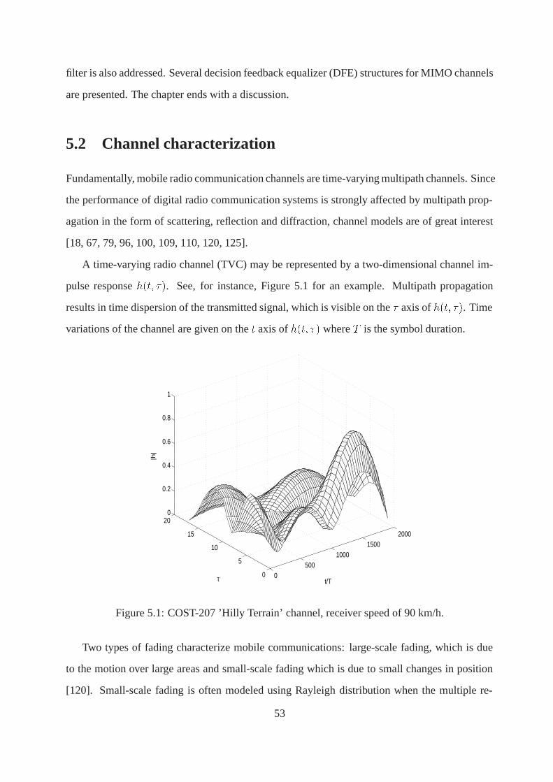
filter is also addressed. Several decision feedback equalizer (DFE) structures for MIMO channels
are presented. The chapter ends with a discussion.
5.2 Channel characterization
Fundamentally, mobile radio communication channels are time-varying multipath channels. Since
the performance of digital radio communication systems is strongly affected by multipath prop-
agation in the form of scattering, reflection and diffraction, channel models are of great interest
[18, 67, 79, 96, 100, 109, 110, 120, 125].
A time-varying radio channel (TVC) may be represented by a two-dimensional channel im-
pulse response���� ��. See, for instance, Figure 5.1 for an example. Multipath propagation
results in time dispersion of the transmitted signal, which is visible on the� axis of���� ��. Time
variations of the channel are given on the� axis of���� �� where� is the symbol duration.
0500
10001500
2000
0
5
10
15
200
0.2
0.4
0.6
0.8
1
t/Tτ
|h|
Figure 5.1: COST-207 ’Hilly Terrain’ channel, receiver speed of 90 km/h.
Two types of fading characterize mobile communications: large-scale fading, which is due
to the motion over large areas and small-scale fading which is due to small changes in position
[120]. Small-scale fading is often modeled using Rayleigh distribution when the multiple re-
53
flective paths are large in number and if there is no line-of-sight (LOS) signal component, the
envelope of the received signal may be statistically described by a Rayleighpdf. When there is a
dominant non-fading component, such as a LOS propagation path, the small-scale fading enve-
lope is modeled as a Riceanpdf. As the amplitude of the non-fading component approaches zero,
the Riceanpdf approaches a Rayleighpdf. The Ricean distribution is often described in terms
of a parameter0. This is also known as the Ricean factor and completely specifies the Ricean
distribution as it is defined as the ratio between the deterministic signal power and the variance
of the multipath [110].
In wireless communications many physical factors in the radio propagation channel cause
fading. Typically there is no LOS path between the mobile units and the base station. Conse-
quently, the received signal consists of multiple copies of the transmitted signal that arrive at the
receiver through different indirect paths. When LOS is present, the channel can be modeled as
containing an LOS component and also as containing multipath components, as we will see later
in this chapter. The randomly distributed amplitudes, phases and arrival angles of these mul-
tipath copies of the transmitted signal cause fluctuations in the received signal power, thereby
introducing fading. In addition to (multipath) fading, multipath propagation also lengthens the
time required for the main portion of the transmitted signal to reach the receiver. This phe-
nomenon is quantified by maximum excess delay��!. In the case of a single transmitted signal
waveform��! represents the time between the first and the last received component. Depending
on the relative durations of the maximum excess delay and the symbol period, multipath fading
is conventionally classified into either frequency-flat fading or frequency-selective fading [120].
Multipath fading is frequency-selective when the symbol period is smaller than the maximum
excess delay. Thus the channel induces intersymbol interference (ISI). The fading is flat when all
the received multipath components arrive within the symbol period. The coherence bandwidth
�� is a measure of the range of frequencies over which the channel response can be considered
“flat”. In other words, coherence bandwidth is the range of frequencies over which two frequency
components have a strong potential for amplitude correlation [110].
Other causes of fading are the frequency offsets between two sources. The signal from one
source undergoes Doppler shift due to relative motion between a transmitter and a receiver. Also,
54
there may be a carrier frequency mismatch between transmit and receive oscillators. Frequency
offsets result in frequency modulation on the transmitted signal, and thereafter cause channel
time-variations that are quantified by coherence time. Depending on the relative values of the
coherence time�" and the symbol period, a fading channel can be categorized either as time-flat
when the symbol period is much less than the channel coherence time. Otherwise, it is time-
selective.
Frequency-selectivity and time-selectivity are two different properties of a fading channel.
Taking into account combinations of time-selectivity and frequency-selectivity, fading channels
are conventionally categorized into one of the following four types:
� Flat fading channels (channels are both time- and frequency-flat).
� Frequency-selective fading channels (channels are frequency-selective but time-flat).
� Time-selective fading channels (channels are time-selective but frequency-flat).
� Doubly-selective fading channels (channels are both frequency- and time-selective).
The wide sense stationary uncorrelated scattering (WSSUS) linear time-variant channel model
is widely used to model signal propagation in mobile communications environment. The WS-
SUS model was introduced by Bello [18] and it was further investigated, for example in [60].
According to [60], the following model can be written:
������ �� �����
������
+���#����$�%��� � �� � ���� (5.1)
where�� is the number of echo paths,��� is the Doppler spread,/� is the angular spread and
� � ��� is the impulse response of the receive filter. For each delay� , the channel is given by
selecting:
1. �� Doppler frequencies��� from a random variable with classical Jakes pdf in�����!� ���!�.The maximum Doppler spread can be expressed like���! � .&��, where. is the mobile
station speed and�� is the signal wave length.
2. �� initial phases/� from a uniform distributed random variable in�� �%.
55
3. �� echo delay times��. Each delay spread is a random variable with probability density
function proportional to the mean power delay profile of the propagation environment.
The uncorrelated scattering assumption leads to an FIR channel model in which all the taps vary
independently of one other. That is, the time-variations of the tap coefficients are mutually uncor-
related while exhibiting the same time-correlation behavior. The physical situation underlying
this model is the existence of a few large scatterers far from the mobile receiver and the exis-
tence of a small number of scatterers in the vicinity of the mobile receiver. Classical analysis of
digital transmission through a fading medium models� ����� �� as zero mean random variables.
In certain applications, such as cellular communications, a direct non-fading path may also ex-
ist, superimposed on the fading path. In this case, the coefficients������ �� have non-zero mean
(Rician fading). The overall non-zero mean channel is then [34, 128]:
������� �� � ������� � ������ ��� (5.2)
where������� is a constant mean and� ������ �� � �.
As pointed out in [93], accurate mathematical channel models are based on collected mea-
surements of actual channels. The COST-207 final report [100] defines propagation channels
that appear in GSM systems. Measurements have been made over typical bandwidths of 10 to 20
MHz at or near 900 MHz. Four propagation environments are described in the project: Typical
Urban (TU), Bad Urban (BU), Hilly Terrain (HT) and Rural Area (RA), each of them having spe-
cific parameter sets. These COST-207 propagation environments are determined by individual
delay distributions that are piecewise exponential functions. A summary of COST-207 channel
parameters is presented in Appendix 1. With these parameters defined, various COST-207 TVCs
can be modeled. A MATLAB implementation of COST-207 model was presented in [19]. It
is also important to mention that COST-207 played an important role in supporting the Group
Special Mobiles in their work that lead to the original design of the Global System for Mobile
Communications (GSM).
Several other COST [95] projects have been active in the area of channel modeling. The
major goals of COST 259 [98] was devoted to an area of huge expansion in telecommunications,
that of high-rate wireless data transmission. Three main areas were addressed, namely radio
56
systems, antennas and propagation and network aspects. Final models and algorithms have been
achieved and many results have been obtained including techniques for OFDM transmission,
enhancement of TDMA systems, and near-far resistant techniques in CDMA. Also directional
radio channels for which indoor/outdoor measurements have been taken were characterized and
adaptive antennas for GSM and wideband CDMA were analyzed.
Projects like COST 273 [101] are curently active. The main objective of this action is to
increase knowledge of the radio aspects of mobile broadband multimedia networks, by exploring
and developing new methods, models, techniques, strategies and tools to further the implemen-
tation of fourth generation mobile communication systems.
Other COST projects (COST 227, COST 231 & COST 280) have the goal of defining feasible
systems for mobile communications based on integration of satellite and terrestrial networks
[97, 101, 99]. In these projects one of the tasks is deriving a channel model for Earth-satellite
and terrestrial paths above about 20 GHz.
Classical channel models provide information on signal power level distribution, Doppler
shifts of received signals. Modern spatial channel models incorporate concepts as time delay
spread, Angle Of Arrival or adaptive antenna geometries [88, 106]. An overview of spatial
channel models is presented in [41], research on channel models has been done also at AT&T
Labs [135], several other models are presented in special issues of technical journals, such the
one in [125].
5.3 Recursive Channel Estimation
Training-based channel estimation consists of classical techniques that estimate the channel from
a known training sequence and observed channel outputs. The mode of operation is “train-before-
transmit”[132], which is effective when the channel does not have significant time variations. In
most cases, training methods appear as robust methods but present some disadvantages. For
example, the effective data rate decreases as a non-negligible portion of a data packet is devoted
to training symbols [35]. In GSM, about 20% of the bits in a burst are used for training.
Blind equalization techniques [79] allow the estimation/equalization of the channel or the
57
equalizer based only on the received data without any training symbols. In other words, the
channel estimation is performed while information symbols are being transmitted, hence, it is a
“train-while-transmit”-type of transmission [132]. The major advantage of this type of transmis-
sion is the improved effective data rate. One drawback is that blind channel estimates converge
slowly from random initial tap values. In rapidly time-varying channel conditions we need to
have some information about the system (e.g. a small number of transmitted symbols) at least for
initialization purposes. In the case of deep fades, the channel tracking algorithm may fail. Thus
we need some new information in order to restore tracking after the fade. In blind methods, some
ambiguities always remain (e.g. rotation of the constellation pattern), and some channels may be
unidentifiable (for example if subchannels in SIMO model have common zeros).
Perhaps one of the best definitions of the notion ofsemi-blind channel estimation/equalization
is given by referring to the use of the known information. Training sequence (TS) methods base
the parameter estimation only on the received signal containing known symbols. All of the
other observations, which may contain unknown symbols, are ignored [35]. Blind methods are
based on all the received data and on knowledge of the structural and statistical properties of the
transmitted data, but not on explicit knowledge of input symbols. For example, it may be known
that the symbols have the property of constant modulus or are i.i.d.
The purpose of semi-blind methods is to combine the benefits of both training sequence-based
and blind methods. Semi-blind techniques, due to the fact that they incorporate the information of
known symbols, avoid the possible pitfalls of blind methods and with only a few known symbols,
any channel, SISO or MIMO, becomes identifiable [35, 85]. Semi-blind techniques appear very
interesting from a performance point of view, as their performance can be superior to that of TS
or blind techniques separately. Semi-blind techniques may be applicable in cases in which TS
and blind methods fail individually [35]. This may be the case of fast TVC when TS and blind
methods cannot estimate and track the channel, especially when deep fades occur, but semi-blind
techniques can offer a viable solution.
Different choices are available for implementing channel estimation and equalization, de-
pending on the channel modeling and on the complexity allowed for each task. Recursive algo-
rithms are needed in order to perform real-time computation and to avoid recomputing everything
58

at the arrival of new symbol. From the family of recursive algorithms, Kalman filter algorithms
offer the best results in terms of channel estimation and tracking under the assumption of states
which obey the Gauss-Markov model, the linearity of the model and known noise statistics. In
highly demanding scenarios (i.e. high speed of the receiver) Kalman filter algorithms offer a
good tradeoff between complexity and performance. They have been successfully applied to the
problem of channel estimation in [66, 82, 128] and in papers" and" !.
5.3.1 Kalman filter for channel tracking
Regular Kalman filters have been applied in SISO and MIMO channel estimation [81, 82, 119].
The state-space model for MIMO channels may be written as:
+��� � �+�� � �� ���� � �� (5.3)
���� � �!���+��� � �����
where�! is a�� �� data matrix defined as:
����� � �������� � � � ������� � � � ���� � �� ���� � � � ���� � �� ����� � (5.4)
� is an� identity matrix and the channel taps are stacked in a vector of length��:
���� ��������� � � � �
������ � � � �
������ � � � �
������ � � � (5.5)
������ ��� � � � ����
�� ��� � � � ������ ��� � � � ����
�� �����
�
Matrix � is the state transition matrix. The condition for applying a conventional Kalman filter
to the model of (5.3) is that the state variables+��� are Gauss-Markov random processes. This is
nearly satisfied in many practical applications for which the channel can be described as Rayleigh
with uncorrelated scattering [66]. Another condition is that the observations are linear, which is
the case of the model from equation (5.3). A Kalman filter [55] can be then applied to the model
of (5.3), leading to an estimate of the state.
5.3.2 Modeling the channel as an AR process
The time correlation of the channel can be exploited in order to allow better channel estimates. A
low-order AR model can be used to describe channel time evolution [14, 66, 128]. An extended
59
Kalman filter (EKF) has been employed in a spread-spectrum SISO environment [66]. The state
vector consisted of the code delay, the Doppler spread, and the tap coefficients. The tap coeffi-
cients were assumed to be uncorrelated. EKF has been employed due to the nonlinear nature of
the measurement equation. The channel was modeled as a first-order AR model and an extension
to order-� AR models was also presented. However, the derivation and analysis of the algorithm
were for the first-order AR case and no method for estimating the state transition matrix (which
contained the AR parameters) was given. The most important fact is that the channel was con-
sidered to be WSSUS, thus only time-correlation of the individual channels was exploited by the
AR model.
The uncorrelated scattering assumption was removed in [128, 129], where the problem of
estimating fading channel environments with correlated coefficients in a SISO case was consid-
ered. The key part of the work in [14, 128, 129] was modeling the channel as a multichannel AR
process of order�. This leads to the following expression for the state equation:
+� ������
��+��� ���� (5.6)
where+� � ���� � � � ����� are the channel taps,�� is a i.i.d. circular complex Gaussian
vector and the matrix�������� is a� � � matrix containing the unknown model coefficients. In
order to simplify the application of a Kalman filter, the following state-space model may to be
built:
�+��� � ����+� � ,�� (5.7)
4� � �����+� � .�� (5.8)
where�+� ��+�� � � � +������
��,�� � 2� � � � � �� and, � � � � � �. The data vector is
defined as��� ����� -� � � � -� �� where�� � �� ���� � � � ����
� . The state matrix�� is:
�� �
��������
�� �� � � � ��
- � � � -
. . . . . ....
- -
!"""""""##
Given the data4� and��, [128] shows how to estimate���, which contains the AR parameters. It
is argued that in multichannel time-series the AR parameters are uniquely identified by the cor-
60
relation matrices�&&��� � ���+��+
���'
�. By post multiplying (5.6) by�+���' and taking expected
value of both sides, it is found that:
��&&��� �
�����
����&&�� � �� � �
���� � � � �� � � � � �# (5.9)
By solving equation (5.9), the parameter matrices�� are obtained. In order to save computation,
an adaptive gradient method to solve (5.9) and to update��� can be used [128]. However, since
�+ is not directly observed, it follows that solving (5.9) is not a trivial task. In [128] two methods
are proposed for estimating�&&���. One is based on Least Squares (LS) and the other on higher
order statistics (HOS). The parameters of interest are the estimates of the��� �� element of the
matrix�&&��� for � � �� � � � � �:
�&&������ � �&�� ! �� �� � � ��� �� � � �� � � � � � � � (5.10)
�&�� ! �� ��def� �
������
���'��
�# (5.11)
Using the notation�'�$�()def� �&�� ! �� �� � � � �&�� ! �� �� �&�� ! �� �� � � � �&�� !�� ��, it is shown
[128] that the LS solution of the linear regression
4�4���' � ����'�' � �
Æ' � +��' (5.12)
for � � �� � � � � � � � will yield an unbiased estimate of�'�$�() under some very general as-
sumptions, where����' � �������� � ��� # # # � �������� � � � ��� ��� � ������ � ��� # # # �
��� � ������ � � � ��. In (5.12), the estimation error is given by+��' � 4�4���'��
�4�4
���' ����
�.
Another method for estimating the lags�&��� � ��� employs HOS. Closed-form expressions
for the tap correlations can be derived using fourth order statistics:
��&��� �� �� �
��� ��
������ ! � � ��� �� � � � � �
��� � ��
�������� !� ��� �� � � � � �
� (5.13)
where�� � *5 ��� ��� ���� �
��.
The paper [128] addresses the problem when a LOS component exits. It follows that a mean
component�+ is present according to equation (5.2). Combining (5.2) and (5.8) the following
model is derived:
�4� � �����+� � 4�� (5.14)
61
where�+� � �+ � �+�. The constants�+ can be consistently estimated via LS solution of equation
(5.14), and4� can be recovered. In a more general case, the mean can be modeled as varying
slowly, so that a first order AR process can be used [34] to describe its time evolution. By
combining this with the AR process of order� used for the channel taps, a new state-space
formulation can be written [34].
5.3.3 Estimating noise statistics
As discussed above, the Kalman filter is widely used for channel estimation. Typically, only
assumptions about the linearity of the state-space model and the Gauss-Markov structure of the
state are invoked when speaking about the optimality of the Kalman filter. Very important compo-
nents are assumed known, including the statistics of the state and measurement noises. Optimal
Kalman filtering requires accurate values of these statistics. Hence, in communications it is of
great importance to
estimate these values using the received measurements and possibly the transmitted symbols.
The problem of identification of noise covariances was addressed in [92] where a batch
method was proposed. This method was applied in [118] in the context of SISO equalization
of time-varying channels. It was further extended to an on-line MIMO case in Paper" !!.
The noise estimation algorithm has two stages: covariance estimation and testing for the
whiteness of the innovations. The noise statistics computation is based on a covariance match-
ing method [92]. The measurement noise covariance matrix is found using the theoretical and
estimated covariances of the innovation sequence. By matching these two expressions of the in-
novation covariance and writing the remaining terms in a recursive manner, a recursive formula
for computing the measurement noise covariance matrix can be found. See Paper" !! for details.
The same approach is used for finding a recursive formula for the state noise covariance matrix.
A residual process is defined and by matching its theoretical and sample covariance matrix a
recursive formula for the state noise covariance is derived.
Adaptive methods for estimating the noise statistics were also introduced in [13, 69]. The
method in [13] was based on a Bayesian type of approach and the method derived in [69] on a
correlation matching method. Both methods found the same adaptive update for the observation
62
noise covariance matrix but different formulas for the state noise covariance. A comprehensive
review of parameter estimation techniques related to Kalman filter is given in [91].
A necessary and sufficient condition for a Kalman filter to operate optimally is that innova-
tions sequence is white (zero mean, uncorrelated). A recursive non-parametric method [87, 122]
for testing the whiteness of the innovation process has been applied in paper" !!. In the case of
MIMO channels, components of an innovation vector are assumed to be mutually uncorrelated.
Hence, whiteness of each component is tested individually. New sequences are formed from the
innovation processes taking the sign of their samples [122]. A run is defined as a set of identical
symbols contained between two different symbols. A sequence would be considered non-random
if there are either too many or too few runs and random otherwise.
5.4 Decision Feedback Equalization in MIMO systems
Decision Feedback Equalizer (DFE) has received much attention recently in the channel equal-
ization community. This is due to the fact that DFEs structure offer intersymbol interference
(ISI) cancelation with reduced noise enhancement [25, 26]. More of the research has been con-
centrated on the SISO case [25, 26, 61] but there is also research in the MIMO case [6, 139]. A
DFE is a nonlinear equalizer that employs previously detected symbols on the current symbol to
be detected. The use of the previously detected symbols makes the equalizer output a nonlinear
function of the data. Due to the nonlinear feedback nature of DFE, symbol errors introduced
by noise may trigger bursts of errors which can lead to poor symbol error rate (SER) perfor-
mance. Because the DFE uses past source symbol estimates to generate new decisions, finding
the desired parameterization from a cold start, where no information about transmitted symbols
is available, is a difficult task [25].
Let us consider4� to be a received signal at time�. The structure of a SISO DFE is presented
in Figure 5.2. The task of the DFE is to estimate the transmitted symbols���. In the case of
an FIR-DFE, equalization is achieved via feedforward� ����� # # # � ���
��and feedback� �
�$�� # # # � $���� filters yielding soft estimates:
���� �
���*��
�*4��* ����*��
$*����* (5.15)
63
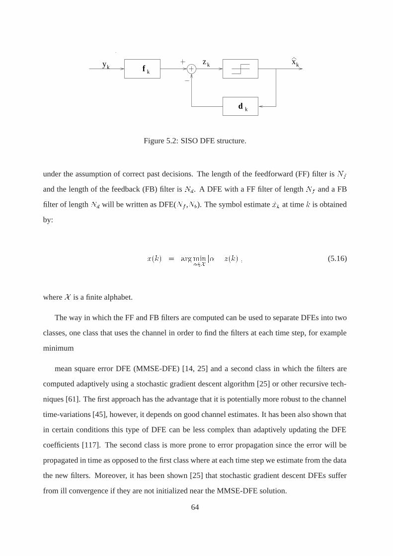
xzyk k kf
d
k
k
Figure 5.2: SISO DFE structure.
under the assumption of correct past decisions. The length of the feedforward (FF) filter is��
and the length of the feedback (FB) filter is�. A DFE with a FF filter of length�� and a FB
filter of length� will be written as DFE(�� ,�+). The symbol estimate��� at time� is obtained
by:
����� � "��#$,��
��� ������ (5.16)
where� is a finite alphabet.
The way in which the FF and FB filters are computed can be used to separate DFEs into two
classes, one class that uses the channel in order to find the filters at each time step, for example
minimum
mean square error DFE (MMSE-DFE) [14, 25] and a second class in which the filters are
computed adaptively using a stochastic gradient descent algorithm [25] or other recursive tech-
niques [61]. The first approach has the advantage that it is potentially more robust to the channel
time-variations [45], however, it depends on good channel estimates. It has been also shown that
in certain conditions this type of DFE can be less complex than adaptively updating the DFE
coefficients [117]. The second class is more prone to error propagation since the error will be
propagated in time as opposed to the first class where at each time step we estimate from the data
the new filters. Moreover, it has been shown [25] that stochastic gradient descent DFEs suffer
from ill convergence if they are not initialized near the MMSE-DFE solution.
64
5.4.1 MIMO MMSE-DFE
Let us start with the definition of the MIMO model used in communications. We will refer to
the model from Figure 2.1. In order to employ the same notation that is commonly used in
equalization community we denote the channel taps using� instead of� and the transmitted
symbols using� instead of�. The rest of the notation remains the same as for the I-MIMO case.
The noise is denoted by. and the received signals by4. The following model is considered:
�� ������
������ � ��� (5.17)
where�� is the�� �th MIMO channel matrix,���� is a� � input vector at time� � � and
� is the maximum length of all of the� channel impulse response, i.e.� � � ���� ������.
A very useful classification was made in [121] where the following terminology was used. If
there are no connections between the filters of different channels it is said to be anon-connected
(NC)-FF/NC-FB a MIMO DFE. If there are connections between the FF and FB filters of each
channel it is said to be afully-connected (FC)-FF/FC-FB a MIMO DFE.
SIMO MMSE-DFE
In this subsection we present an important result which links the SISO case to the MIMO one,
namely the Single Input Multiple Output (SIMO) model. This type of MMSE-DFE was intro-
duced in [25]. The structure of the system is depicted in Figure 5.3. The model used is a special
case of (5.17) with only one antenna at the transmitter. The received signal at antenna� is:
4�� ��+���
���� � .��� (5.18)
where+��� is a�� � vector containing� channel taps of the path�� at time�, �� contains� past
symbols sent by the transmit antenna and. �� is the AWGN at antenna�. The received vector at
time � has the form�� � 4� � � � 4�� . The SIMO MMSE-DFE giving soft decisions��� has the
structure:
��� � ��� �� � ��� (5.19)
������
� ���*��
� ���* 4
�����*
!#�
���*��
$*����*�
65
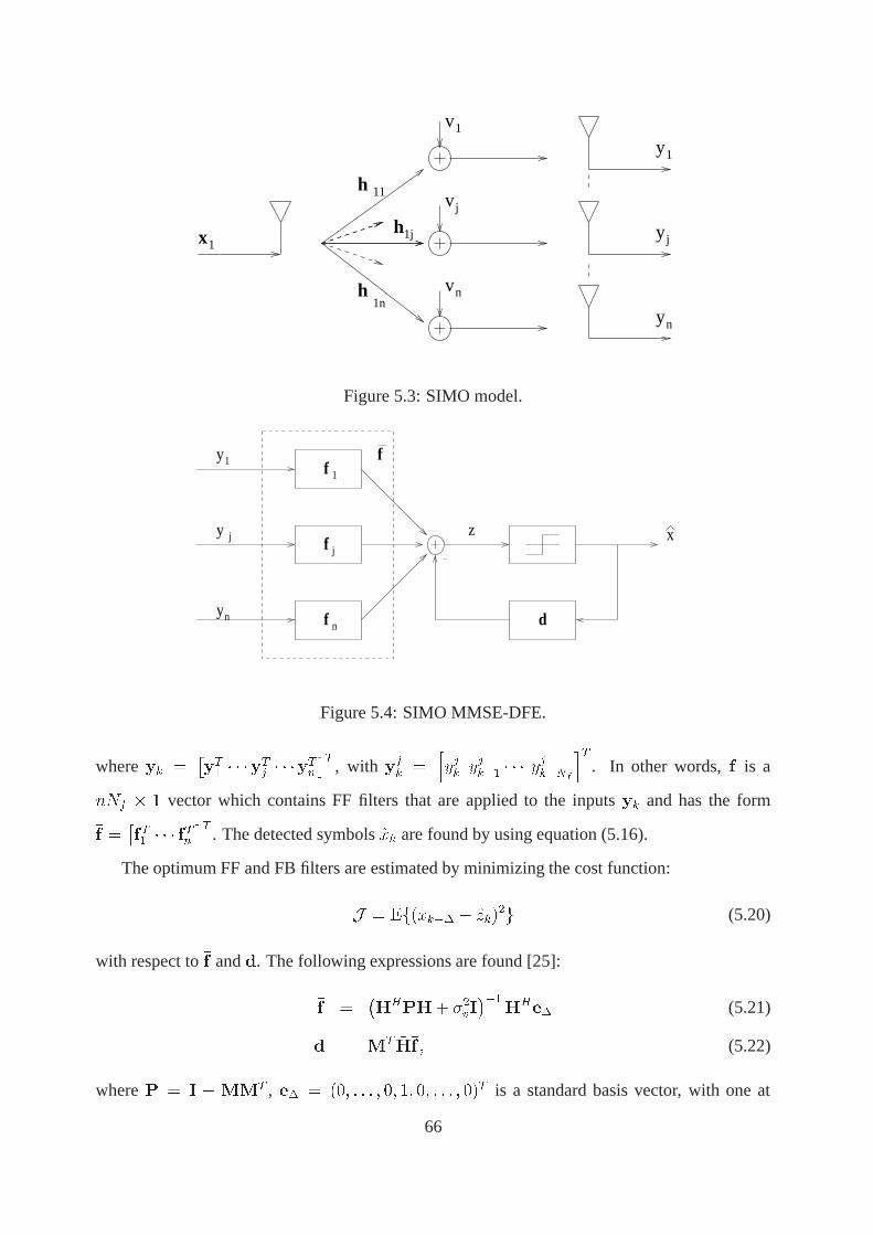
v1
vj
vn
y
y
yn
1
jx
h
h
11
1n
11jh
Figure 5.3: SIMO model.
x
y1
y j
yn
f 1
f
f
j
n d
z
f
Figure 5.4: SIMO MMSE-DFE.
where ��� ����� � � ���� � � ����
��, with �
�� �
�4�� 4���� � � � 4�����
��. In other words,�� is a
��� � � vector which contains FF filters that are applied to the inputs��� and has the form
�� ����� � � � ���
��. The detected symbols��� are found by using equation (5.16).
The optimum FF and FB filters are estimated by minimizing the cost function:
� � ������ � ������ (5.20)
with respect to�� and�. The following expressions are found [25]:
�� ������ ��� �
��� ���� (5.21)
� � .� ���� � (5.22)
where� � �..� , � � ��� # # # � �� �� �� # # # � ��� is a standard basis vector, with one at
66
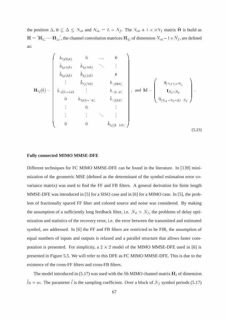
the position�, � � � � �"& and�"& � � � �� . The�"& � � � ��� matrix �� is build as
�� � ��� � � ����, the channel convolution matrices��� of dimension�"&����� , are defined
as:
������ �
��������������������������
��������� � � �
��������� ���������. . .
...
��������� ���������
... ��������� ���������
�����������
... ���������
��������������������
... ...
......
. . ....
�����������
��������������������������
� and � �
������
� ������
������
������� ����
������
�
(5.23)
Fully connected MIMO MMSE-DFE
Different techniques for FC MIMO MMSE-DFE can be found in the literature. In [139] mini-
mization of the geometric MSE (defined as the determinant of the symbol estimation error co-
variance matrix) was used to find the FF and FB filters. A general derivation for finite length
MMSE-DFE was introduced in [5] for a SISO case and in [6] for a MIMO case. In [5], the prob-
lem of fractionally spaced FF filter and colored source and noise was considered. By making
the assumption of a sufficiently long feedback filter, i.e.� ' �� , the problems of delay opti-
mization and statistics of the recovery error, i.e. the error between the transmitted and estimated
symbol, are addressed. In [6] the FF and FB filters are restricted to be FIR, the assumption of
equal numbers of inputs and outputs is relaxed and a parallel structure that allows faster com-
putation is presented. For simplicity, a� � � model of the MIMO MMSE-DFE used in [6] is
presented in Figure 5.5. We will refer to this DFE as FC MIMO MMSE-DFE. This is due to the
existence of the cross-FF filters and cross-FB filters.
The model introduced in (5.17) was used with the�th MIMO channel matrix� � of dimension
��� �. The parameter�� is the sampling coefficient. Over a block of�� symbol periods (5.17)
67
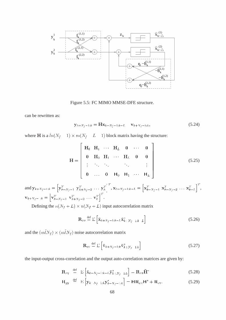
(1,1)f
(2,2)f
e0
e0
xk−
xk−(1,2)f
(2,1)f
zky1
y2
(1)
(2)
−b(1,1)
−b(2,2)
(2,1)−b
−b(1,2)
k
k
k
k
k
k
k
k
k
k
Figure 5.5: FC MIMO MMSE-DFE structure.
can be rewritten as:
���������� � �������������� � ����������� (5.24)
where �� is a������ � ������ � �� �� block matrix having the structure:
�� �
$$$$$$$�
�� �� � � � �� - � � � -
- �� �� � � � �� - -
.... . . . . . . . .
...
- # # # - �� �� � � � ��
�%%%%%%%�
(5.25)
and���������� ���������� �������� # # # ���
��, ������������ �
��������� �
������� # # # �����
��,
���������� ���������� �
������� # # # ���
��.
Defining the���� � ��� ���� � �� input autocorrelation matrix
�def� �
���������������
�����������
�(5.26)
and the����� �� ������ noise autocorrelation matrix
� def� �
�������������
���������
�(5.27)
the input-output cross-correlation and the output auto-correlation matrices are given by:
��def� �
���������������
���������
�� �
��� (5.28)
���def� �
�������������
���������
�� ���
��� �� # (5.29)
68
The FIR MIMO MMSE-DFE consists of an FF filter matrix
��� def����� ��
� � � � ������
�(5.30)
with �� matrix taps��, each of size��� � ��, and an FB filter matrix equal to
� ��������� def
��� � ���
�� ���� � � � ���
�
�# (5.31)
The following matrix is defined [6]:
�� ����
� ��� � � � ��
��
�(5.32)
containing� � � matrix taps��, each of size� � �. Furthermore, the following matrix is
defined: ��� def� -��� ��, where� � � � �� � � � � is the decision delay that satisfies the
condition��� � � � �� � �. The error vector of the MIMO MMSE-DFE at time� is given
by:
��� � ��������������� � ������������# (5.33)
Applying the orthogonality principle, which states that���������������
�� �, the optimum
FF filter matrix is found [6]:
�����$ � ���
��$������� # (5.34)
Using the partitioning�def�
� ��� ���
��� ���
�� where��� is of size�� � ��� �� � ��,
����$ �
� �� ���
�����
����
��(� (5.35)
where(� def� -��� � and� � ���
� ������
��.
Non-connected MIMO MMSE-DFE
In this subsection the MIMO MMSE-DFE derived in Papers" and" ! is briefly presented. This
type of DFE belongs to the NC category, meaning that pairs of feedforward-feedback filters for
each received signal based on the MMSE criterion are computed. The derivation is based on
the assumption that the input and noise processes are uncorrelated. This scheme has also lower
computational complexity.
69
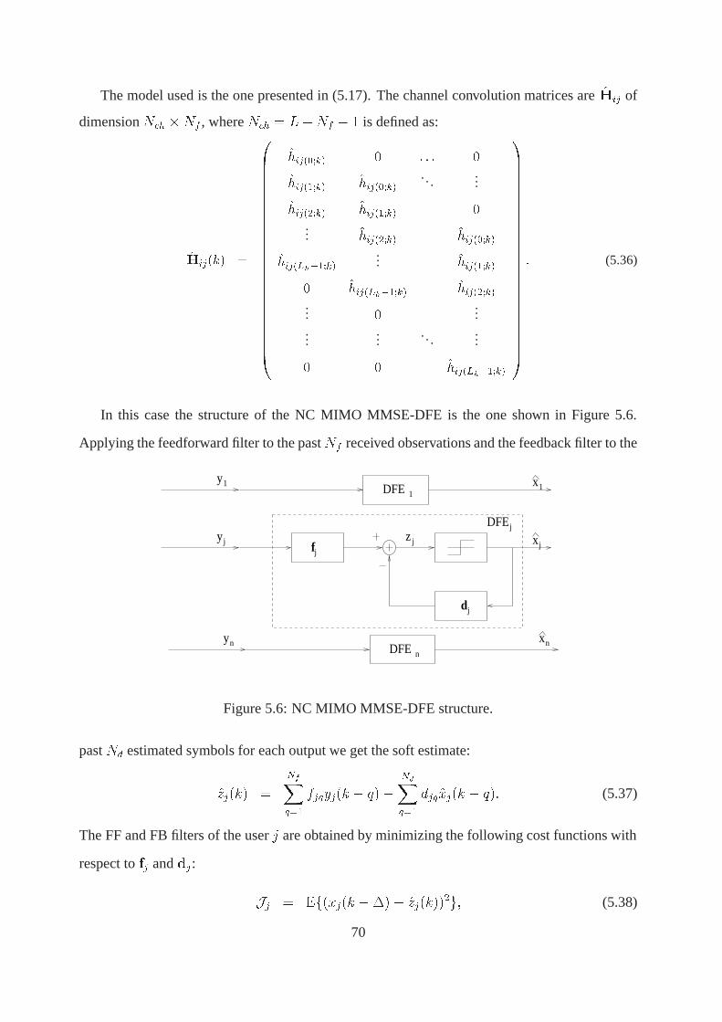
The model used is the one presented in (5.17). The channel convolution matrices are���� of
dimension�"& ��� , where�"& � ���� � � is defined as:
������� �
��������������������������
��������� � � �
��������� ���������.. .
...
��������� ���������
... ��������� ���������
�����������
... ���������
��������������������
... ...
......
.. ....
�����������
��������������������������
� (5.36)
In this case the structure of the NC MIMO MMSE-DFE is the one shown in Figure 5.6.
Applying the feedforward filter to the past�� received observations and the feedback filter to the
x1
xj
x
yj fjz
dj
j
DFEy1
1
DFEj
yn nDFE n
Figure 5.6: NC MIMO MMSE-DFE structure.
past� estimated symbols for each output we get the soft estimate:
������ �
���*��
��*4��� � �����*��
$�*����� � �# (5.37)
The FF and FB filters of the user� are obtained by minimizing the following cost functions with
respect to�� and��:
�� � ������� ���� ���������� (5.38)
70

whereÆ is the equalization delay and����� is given by:
�� � �������� � # # #� ��� ����� � # # #� �������� � ��� �� � ���� ��# (5.39)
In equation (5.38) we assume that past decisions are correct. Moreover, the input sequences
are assumed to be uncorrelated with each other and with the noise.
Let us consider the observation vector received at receiver�. When we calculate the pair
�������, index � is fixed and� is running from�� # # # � �. We use the notation���� ���� for the
case when the indexes� and� are equal. Hence,���� � ���� ���� corresponds to the direct path
channel. Under the above assumptions and notation, for an�� MIMO system we obtain:���� �
������
���� � � � �� ����� ���� �����
���� ���� � � � �� ��������� � ��
�������� ���� �
� � ������ ���� ���
(5.40)
where.� � �-�� �����-��������� �, and����� � � � .�
�.��. Furthermore
� � �-��
and� � ��� # # # � �� �� �� # # # � ��� is the standard basis vector, with a value one at positions
�, � � � � �� . The derivation of the above two equations is presented in Paper" for a �� �
case and in Paper" ! for a general case.
Finally, the symbol estimate��� at time� is obtained from:
������ � "��#$,��
��� �������� (5.41)
where� is a finite alphabet.
5.5 Discussion
Using channel models based on measurements is very important when trying to simulate real
communications environments. COST 207 is an effective model based on measurements of ac-
tual outdoor channels. These measurement-based power delay profiles and Doppler spectra of
outdoor channels are useful in testing estimation and equalization algorithms. Different models
have to be used if one wants to perform simulations in indoor environments, for example [93].
Nevertheless, for more advanced mathematical channel models one should consider recent COST
[95] projects, such as COST 231, COST 259, COST 273 [96, 98, 101], as well as recent models
proposed in technical journals, such as those in [3, 41, 135].
71
Joint channel tracking and equalization algorithms can perform well in the face of time-
varying channels. In fact they outperform conventional adaptive equalization algorithms, such
as LMS or RLS algorithms, which do not explicitly incorporate quasi-invariant channel statistics
such as Doppler rate and the channel mean. This quantities may be known to the receiver as a
result of prior processing. Channels which change rapidly can be tracked continuously. Hence,
Kalman filters can be used as optimal channel estimators [14, 123]. The performance of a DFE
coupled with LMS or RLS channel estimators was analyzed for a SISO channel model in [14,
117].
As shown in [128], fitting a crude model of channel time variation is better than no model at
all. However, the complexity of the receiver increases relative to that of ordinary Kalman filtering
techniques because multiple matrices of AR coefficients have to be estimated at every re-training
of the algorithm. A good trade-off between complexity and performance is obtained using a
simpler model. A low order AR model or even a simple Markov model can capture most of the
channel tap dynamics and lead to effective tracking algorithms [83]. When using a Kalman filter
for channel estimation and tracking, the system must include a noise estimation stage because
noise statistics are not knowna priori and may vary in time. Errors in channel estimation result
in additional DFE performance degradation. This problem has been studied in [123].
Linear equalizers are best suited for channels which vary slowly. Deep frequency-selective
fades are a characteristic of some common wireless channels. For such channels, DFEs are gen-
erally preferred to linear equalizers, since their complexity is comparable and their performance
suffers less under amplitude distortion. Assuming perfect knowledge of the MIMO channel, the
optimum receiver is a maximum likelihood sequence estimator (MLSE), but its complexity is
prohibitive, even for low-order channels with a small number of inputs and outputs [124].
Equalization performed with a DFE gives a good trade-off between performance and com-
plexity, compared to equalization with an optimal Viterbi algorithm. We believe that is an
open discussion on advantages/disadvantages issues with respect to to fully-connected and non-
connected MIMO MMSE-DFE structures. The equalizers are derived using different approaches,
so it is difficult to make a fair comparison. However, the performance may depend on angular
spread [135]. This implies that for mobile stations and for indoor base stations the angular spread
72

is high (almost���Æ) [135], thus low correlation can be achieved and NC MIMO DFE may give
good results. In scenarios where the angular spread is low, and the spacing between antennas is
not of a few wavelength in order to assure low correlation, a fully-connected MIMO DFE may
perform better since it exploits this correlations. One drawback of the DFE structure may be the
fact that errors may occur in bursts due to the fed-back symbol estimates and may lead to poor
equalization.
Adaptive algorithms need acquisition and tracking phases. During acquisition, the initial val-
ues of the parameters are estimated. Usually acquisition is done with a known training sequence.
Tracking may be needed in a time-varying channel to update the estimates obtained during the
acquisition phase. The results from the literature in both SISO [14, 123] and MIMO [83] scenar-
ios and also our simulation results validate the assumption that in the case of joint tracking and
equalization algorithms, Kalman filter techniques offer the best channel tracking performance
and DFE structure is a good tradeoff between complexity and performance.
73

74
Chapter 6
Summary
Blind source separation methods allow solution of many difficult signal processing problems
in different application domains. Blind techniques are very important in applications for which
there are sets of recorded data or observations, but little or no other information about specific pa-
rameter values of the system which produced the observations. An example is the measurement
of multiple electroencephalogram traces, where sensor recordings are available, but no model
for the brain signals which contribute to the traces. Blind techniques can produce very practi-
cal results. For instance, in communications, spectrum is a scarce resource and there is a need
for higher data rates. Blind receivers require no training and allow transmission of user data
in place of training sequences. On the other hand, communications receivers have to achieve
high performance in demanding environments. Fully blind receivers may suffer from slow con-
vergence and may have ambiguities. Hence,semi-blind algorithms have been introduced [35].
Semi-blind algorithms combine blind techniques and short training sequences, as well as other
known information. Such algorithms can show improved performance relative to blind methods
in challenging environments. They represent a practical alternative to training-based methods.
In this thesis a blind recursive method for solving the separation problem of linear instanta-
neous mixing was proposed. The possibilities of time-varying mixing matrices and noise were
taken into account. The changes that may occur in the signal subspace were also considered and
it was shown that they can be tracked on-line. A sample covariance matrix computed over a small
window compared with the covariance matrix of the subspace revealed changes in the signal sub-
75
space. This was due to the high fluctuations in the correlation difference between the window
estimate and the subspace covariance matrix. A simple thresholding was used to determine a
change in environment and the subspace tracker was reinitialized. In a blind equalization appli-
cation, fractional sampling was used to convert a finite input response multiple-input multiple-
output (FIR-MIMO) model into a instantaneous multiple-input multiple-output (I-MIMO) model.
The thesis showed that this technique allows recursive blind source separation to be applied to
equalization of slowly time-varying channels.
The blind equalization work reported in this thesis has provided new solutions for the more
challenging problem of MIMO equalization of time-varying channels. State-space models were
useful for modeling time-varying systems. Recursive estimation was a natural way to deal with
such models and was a key element of the methods developed in this work. Interestingly, the
recursive techniques developed here were related to Kalman filter, which even four decades after
its invention proves to be a valuable tool. Kalman filtering was the subject of active research in
control theory in 60’s. Demanding wireless communication applications of the 21�� century may
bring it back into the spotlight. There are still important aspects of Kalman filters which deserve
closer attention. For example, solutions to the noise estimation problem can be very useful if
one wants to have close to optimal algorithms which require little known information. In this
work a solution for real-time noise estimation was presented based on testing the whiteness of
innovations.
This thesis showed that a semi-blind technique can be used for equalization of MIMO time-
varying channels. The algorithm derived for this purpose was based on a state-space model and
recursive estimation. It worked in two stages, first estimating the channel and then equalizing it.
A short training sequence was supplied for initializing a channel tracker. Subsequently, the algo-
rithm worked in a decision-directed mode, meaning that the symbols from the equalization part
were fed back and used to update the channel estimate. The channel estimation stage was based
on Kalman filtering and included a noise estimation stage. This resulted in near-optimal channel
estimation. The equalization was based on a non-connected MIMO minimum mean square error
- decision feedback equalizer (MMSE-DFE) structure. In this structure, an independent DFE
operated on each sensor. Simulation results showed that the algorithm was able to track changes
76
in time-varying channels and also to reduce intersymbol and interuser interference. It was also
shown that the state and observation noise covariances can be successfully identified.
One possible topic of future research is closer analysis of the FIR-MIMO equalization prob-
lem. The channel tracking stage should be made robust to error bursts. These investigations
may provide guidelines for the design of optimal training sequences that enable fast, accurate
recovery following deep fades. The noise estimation stage needs careful understanding as it is
critical to the performance of the Kalman filter. Erroneous estimates of the noise covariances can
seriously impair Kalman filter behavior. Another important aspect of Kalman filtering is choice
of the state transition matrix. Usually this matrix is assumed to be known and almost an identity
matrix. Sometimes it is treated as having autoregressive parameters. However, more investiga-
tion is needed to determine if these assumptions are valid. A closer investigation of the interuser
interference cancellation problem should be performed. The influence of user signal power on
the performance of the non-connected MIMO MMSE-DFE should be investigated. Further solu-
tions should be considered to improve the performance of the equalizer. For example, combining
space-time coding with semi-blind equalization may lead to robust algorithms. Extension of
blind methods applied to multicarrier systems would also be useful.
77

78

Appendix A
COST 207 model
The following four types of Doppler spectra are defined in the COST 207 model [100] and can
be also found in [93]:
1. CLASS - classical Jakes Doppler spectrum used for paths with delays not in excess of 500
ns.
2. GAUS 1 - is a sum of two Gaussian functions and is used for excess delay times in the
range of 500 ns to 2�s.
3. GAUS 2 - is a sum of two Gaussian functions and is used for paths with delays equal or
more than 2�s.
4. RICE - is the sum of a classical Doppler spectrum and one direct path, such that the total
multipath contribution is equal to that of the direct path. This spectrum is used for the
shortest path of the model for propagation in RA.
The way in which these Doppler spectra should be applied to the four propagation classes is
shown in Tables A.1-A.4.
79
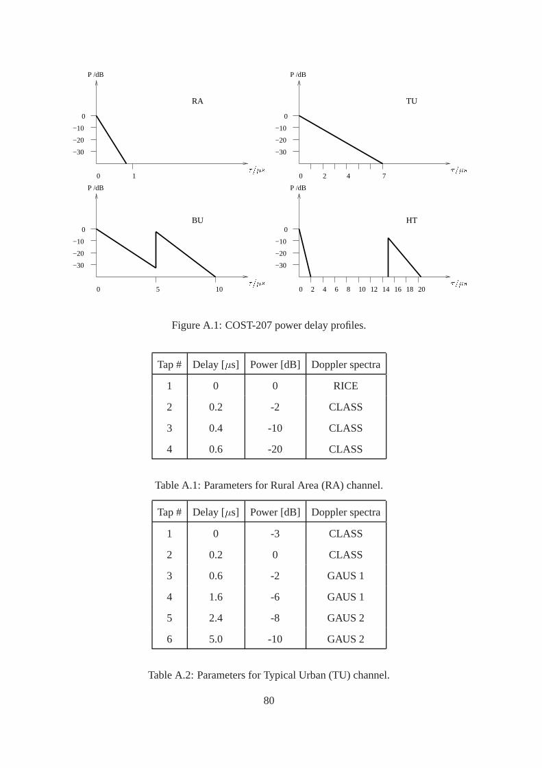
P /dB
0
−10
−20
−30
P /dB
0
−10
−20
−30
P /dB
0
−10
−20
−30
P /dB
0
−10
−20
−30
2 4 7010
05 10 2 4 6 20181614121080
RA
BU
TU
HT
�&�� �&��
�&���&��
Figure A.1: COST-207 power delay profiles.
Tap # Delay [�s] Power [dB] Doppler spectra
1 0 0 RICE
2 0.2 -2 CLASS
3 0.4 -10 CLASS
4 0.6 -20 CLASS
Table A.1: Parameters for Rural Area (RA) channel.
Tap # Delay [�s] Power [dB] Doppler spectra
1 0 -3 CLASS
2 0.2 0 CLASS
3 0.6 -2 GAUS 1
4 1.6 -6 GAUS 1
5 2.4 -8 GAUS 2
6 5.0 -10 GAUS 2
Table A.2: Parameters for Typical Urban (TU) channel.
80
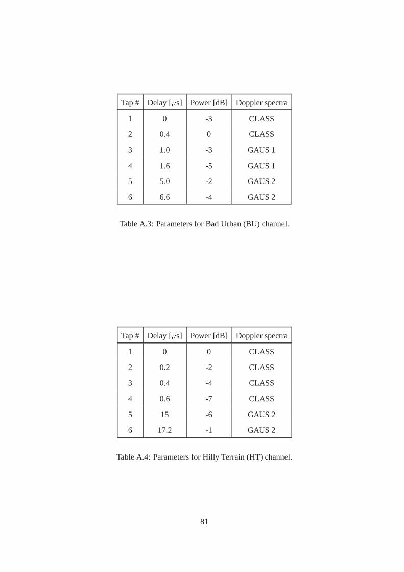
Tap # Delay [�s] Power [dB] Doppler spectra
1 0 -3 CLASS
2 0.4 0 CLASS
3 1.0 -3 GAUS 1
4 1.6 -5 GAUS 1
5 5.0 -2 GAUS 2
6 6.6 -4 GAUS 2
Table A.3: Parameters for Bad Urban (BU) channel.
Tap # Delay [�s] Power [dB] Doppler spectra
1 0 0 CLASS
2 0.2 -2 CLASS
3 0.4 -4 CLASS
4 0.6 -7 CLASS
5 15 -6 GAUS 2
6 17.2 -1 GAUS 2
Table A.4: Parameters for Hilly Terrain (HT) channel.
81

82
Bibliography
[1] Blind system identification and estimation. volume 86, pages 1901–2116. Proceedings of
the IEEE, 1998.
[2] Independence and artificial neural networks. volume 22. Neurocomputing, 1998.
[3] Special issue on channel and propagation models for wireless system design I. volume 20,
pages 493–647. IEEE Journal on Selected Areas in Communications, 2002.
[4] Special issue on Monte Carlo methods for statistical signal processing. volume 50, pages
173–449. IEEE Transactions on Signal Processing, 2002.
[5] N. Al-Dhahir and J.M. Cioffi. MMSE decision feedback equalizers: Finite length results.
IEEE Transactions on Information Theory, 41:961–976, 1995.
[6] N. Al-Dhahir and A.H. Sayed. The finite length Multi-Input Multi-Output MMSE-DFE.
IEEE Transactions on Signal Processing, 48(10):961–976, 2000.
[7] S-I. Amari. Natural gradient works efficiently in learning.Neural Computation, 10:251–
276, 1998.
[8] S-I. Amari, T.-P. Chen, and A. Cichocki. Stability analysis of adaptive blind source sepa-
ration. Neural Networks, 10(8):1345–1351, 1997.
[9] S-I. Amari and A. Cichocki. Adaptive blind signal processing-neural network approaches.
Proceedings of the IEEE, 86(10):2026–2048, 1998.
[10] S-I. Amari, A. Cichocki, and H. Yang. A new learning algorithm for blind signal separa-
tion. Advances in Neural Processing Systems, 8:752–763, 1996.
83

[11] S-I. Amari, A. Cichocki, and H.H. Yang. A new learning algorithm for blind signal sepa-
ration. Advances in Neural Information Processing Systems, pages 752–763, 1995.
[12] S-I. Amari, S.C. Douglas, A. Cichocki, and H.H. Yang. Multichannel blind deconvolution
and equalization using the natural gradient.Proceedings of the IEEE Workshop on Signal
Processing and Advances in Wireless Communications, pages 101–104, 1997.
[13] Sage A.P. and Husa G.W. Adaptive filtering with unknown prior statistics.Proceedings of
Joint Automatic Control Conference, pages 760–769, 1969.
[14] Y. Ara and H. Ogiwara. Adaptive equalization of selective fading channel based on
AR-model of channel-impulse-response fluctuation.Electronics and Communications in
Japan, 74(7):76–86, 1991.
[15] M.S. Arulampalam, S. Maskell, N. Gordon, and T. Clapp. A tutorial on particle filters for
online nonlinear/non-Gaussian Bayesian tracking.IEEE Transactions on Signal Process-
ing, 50(2):174–188, 2002.
[16] H. Attias. Independent factor analysis.Neural Computation, 11:803–851, 1999.
[17] A. J. Bell and T. J. Sejnowski. An information-maximisation approach to blind separation
and blind deconvolution.Neural Computation, 7(6):1129–1159, 1995.
[18] P.A. Bello. Characterization of randomly time-variant linear channels.IEEE Transactions
on Communications Systems, 11(4):360–393, 1963.
[19] D. Boss, K-D. Kammeyer, and T. Petermann. Is blind channel estimation feasible in
mobile communications systems? a study based on GSM.IEEE Journal on Selected
Areas in Communications, 16(8):1479–1492, 1998.
[20] J-F. Cardoso. Source separation using higher order moments.Proceedings of ICASSP,
pages 2109–2112, 1989.
[21] J-F. Cardoso. Blind signal separation: Statistical principles.Proceedings of the IEEE,
86(10):2009–2025, 1998.
84
[22] J-F. Cardoso. High-order contrasts for Independent Component Analysis.Neural Compu-
tation, 11(1):157–192, 1999.
[23] J-F. Cardoso and B. Laheld. Equivariant adaptive source separation.IEEE Transactions
on Signal Processing, 44:3017–3030, 1996.
[24] J-F. Cardoso and A. Souloumiac. Blind beamforming for non-Gaussian signals.IEE
Proceedings F, 140(6):362–370, 1993.
[25] R.A. Casas, T.J. Endres, A. Touzni, C.R. Johnson Jr, and J.R. Treichler. Current ap-
proaches to blind decision feedback equalization. In G.B. Giannakis, Y. Hua, P. Stoica,
and L. Tong, editors,Signal Processing Advances in Wireless and Mobile Communica-
tions, Volume 1: Trends in Channel Estimation and Equalization. Prentice Hall, 2000.
[26] R.A. Casas, P.B. Schniter, J. Balakrishnan, C.R. Johnson, Jr. Berg, and C.U. Berg.DFE
Tutorial, 1998.
[27] C.K. Chui and G. Chen.Kalman Filtering with Real-Time Applications. Springer, 3rd
edition, 1999.
[28] A. Cichocki and S-I. Amari. Adaptive Blind Signal and Image Processing : Learning
Algorithms and Applications. Wiley, 2002.
[29] A. Cichocki and L Zhang. Two-stage blind deconvolution using state-space models.Pro-
ceedings of ICONIP, pages 729–732, 1998.
[30] P. Comon. Independent Component Analysis – a new concept?Signal Processing,
36(3):287–314, 1994.
[31] P. Comon and P. Chevalier.Unsupervised Adaptive Filtering, Vol. I: Blind Source Separa-
tion, chapter Blind Source Separation: Models, Concepts, Algorithms, and Performance.
John Wiley & Sons, 2000.
[32] P. Comon and G. H. Golub. Tracking a few extreme singular values and vectors in signal
processing.Proceedings of the IEEE, 78(8):1327–1343, 1990.
85
[33] R. Cristescu, T. Ristaniemi, J. Joutsensalo, and J. Karhunen. Blind separation of convolved
mixtures for CDMA systems.European Signal Processing Conference, EUSIPCO, pages
619–622, 2000.
[34] L.M. Davis, I.B. Collings, and R.J. Evans. Coupled estimators for equalization of fast-
fading mobile channels. IEEE Transactions on Communications, 46(10):1262–1265,
1998.
[35] E. de Carvalho and D. Slock. Semi-blind methods for FIR multichannel estimation. In
G.B. Giannakis, Y. Hua, P. Stoica, and L. Tong, editors,Signal Processing Advances
in Wireless and Mobile Communications, Volume 1: Trends in Channel Estimation and
Equalization. Prentice Hall, 2000.
[36] S. C. Douglas. Combined subspace tracking, prewhitening, and contrast optimization for
noisy blind signal separation.Proceedings of the Independent Component Analysis and
Blind Signal Separation Workshop (ICA 2000), pages 579–584, 2000.
[37] S. C. Douglas. Numerically-robust adaptive subspace tracking using householder trans-
formations.IEEE Sensor Array Multichannel Workshop, pages 499–503, 2000.
[38] S. C. Douglas. Handbook of Neural Network Signal Processing, chapter Blind Signal
Separation and Blind Deconvolution. CRC Press, 2001.
[39] S. C. Douglas, A. Cichocki, and S-I. Amari. Multichannel blind separation and decon-
volution of sources with arbitrary distributions.IEEE Workshop on Neural Networks for
Signal Processing, pages 436–445, 1997.
[40] S.C. Douglas and S. Haykin.Unsupervised Adaptive Filtering, Vol. II: Blind Deconvo-
lution, chapter Relationships between Blind Deconvolution and Blind Source Separation.
John Wiley & Sons, 2000.
[41] R.B. Erdel, P. Cardieri, K.W. Sowerby, and T.S. Rappaport. Overview of spatial channel
models for antenna array communications.IEEE Personal Communications Magazine,
5(1):10–22, 1998.
86
[42] R. Everson and J. S. Roberts. Non-stationary Independent Component Analysis.Interna-
tional Conference on Artificial Neural Networks, pages 503–508, 1999.
[43] R. Everson and J. S. Roberts, editors.Advances in Independent Components Analysis.
Kluwer Academic Publishers, 2000.
[44] R. Everson and J. S. Roberts.Independent Component Analysis Principles and Practice.
Cambridge University Press, 2001.
[45] S.A. Fechtel and M. Meyr. An investigation of channel estimation and equalization tech-
niques for moderately rapid fading HF-channels.Proceedings of the International Con-
ference on Communications, pages 768–772, 1991.
[46] A. B. Gharbi and F. M. Salam. Algorithms for blind signal separation and recovery in
static and dynamic environments.IEEE International Symposium on Circuits and Systems,
1:713–716, 1997.
[47] G.B. Giannakis, Y. Hua, P. Stoica, and L. Tong, editors.Signal Processing Advances
in Wireless and Mobile Communications, Volume 1: Trends in Channel Estimation and
Equalization. Prentice Hall, 2000.
[48] X. Giannakopoulos, J. Karhunen, and E. Oja. An experimental comparison of neural ICA
algorithms with real-world data.Proceedings of the International Joint Conference on
Neural Networks (IJCNN’99), pages 888–893, 1999.
[49] M. Girolami. An alternative perspective on adaptive Independent Component Analysis
algorithms.Neural Computation, 10(8), 1998.
[50] M. Girolami. Noise reduction and speech enhancement via temporal anti-hebbian learning.
Proceedings of ICASSP, 1998.
[51] M. Girolami, editor.Self-Organising Neural Networks - Indepedent Component Analysis
and Blind Source Separation. Springer-Verlag, 1999.
87
[52] D.N. Godard. Self-recovering equalization and carrier tracking in two-dimensional data
communication systems.IEEE Transactions on Communications, 28(11):1867–1875,
1980.
[53] N.J. Gordon, D.J. Salmond, and A.F.M. Smith. Novel approach to nonlinear/non-Gaussian
Bayesian state estimation.IEE Proceedings-F, pages 107–113, 1993.
[54] A. Gorokhov, P. Loubaton, and E. Moulines. Second order blind equalization in multiple
input multiple output FIR systems: a weighted least squares approach.Proceedings of
ICASSP, 5:2415–2418, 1996.
[55] S. Haykin.Adaptive Filter Theory. Prentice-Hall, 3rd edition, 1996.
[56] S. Haykin, editor.Unsupervised Adaptive Filtering, Vol. I, Blind Source Separation. Wiley,
2000.
[57] S. Haykin, editor.Unsupervised Adaptive Filtering, Vol. II, Blind Deconvolution. Wiley,
2000.
[58] J. Herault and C. Jutten. Blind separation of sources, part II: Problem statement.Signal
Processing, 24(1):11–20, 1991.
[59] J. Herault, C. Jutten, and B. Ans. D´etection de grandeurs primitives dans un message
composite par une architecture de calcul neuromim´etique en apprentissage non supervis´e.
Proc. Xeme colloque GRETSI, pages 1017–1022, 1985.
[60] P. Hoeher. A statistical discrete-time model for the WSSUS multipath channel.IEEE
Transactions on Vehicular Technology, 41(4):461–468, 1992.
[61] F.M. Hsu. Square root Kalman filtering for high-speed data received over fading dispersive
HF channels.IEEE Transactions on Information Theory, 28(5):753–763, 1982.
[62] Y. Hua. Fast maximum likelohood for blind identification of multiple FIR channels.IEEE
Transactions on Signal Processing, 44(3):661–672, 1996.
88
[63] A. Hyvarinen. A family of fixed-point algorithms for Independent Component Analysis.
Proceedings of ICASSP, pages 3917–3920, 1997.
[64] A. Hyvarinen. Fast and robust fixed-point algorithms for Independent Component Analy-
sis. IEEE Transactions on Neural Networks, 10(3):626–634, 1999.
[65] A. Hyvarinen, J. Karhunen, and E. Oja.Independent Component Analysis. Wiley, 2001.
[66] R.A. Iltis. Joint estimation of PN code delay and multipath using the extended Kalman
filter. IEEE Transactions on Communications, 38(10):1677–1685, 1990.
[67] W.C. Jakes.Microwave Mobile Communications. Wiley, 1974.
[68] C. Jutten and J. Herault. Blind separation of sources, part I: an adaptive algorithm based
on neuromimetic architecture.Signal Processing, 24:1–10, 1991.
[69] Myers K.A. and B.D. Tapley. Adaptive sequential estimation with unknown noise statis-
tics. IEEE Transactions on Automatic Control, 4(21):520–523, 1976.
[70] I. Karasalo. Estimating the covariance matrix by signal subspace averaging.IEEE Trans-
actions on Acoustics, Speech, and Signal Processing, 34(1):8–12, 1986.
[71] J. Karhunen, A. Cichocki, W. Kasprzak, and P. Pajunen. On neural blind separation with
noise suppression and redundancy reduction.International Journal of Neural Systems,
8(2):219–237, 1997.
[72] J. Karhunen and J. Joutsensalo. Representation and separation of signals using nonlinear
PCA type learning.Neural Networks, 1(8):113–127, 1994.
[73] J. Karhunen, E. Oja, L. Wang, R. Vigario, and J. Joutsensalo. A class of neural networks
for Independent Component Analysis.IEEE Transactions on Neural Networks, 8(3):486–
504, 1997.
[74] J. Karhunen and P. Pajunen. Blind source separation and tracking using nonlinear PCA
criterion: A least-squares approach.IEEE International Conference on Neural Network,
pages 2147–2152, 1997.
89
[75] J. Karhunen and P. Pajunen. Blind source separation using least-squares type adaptive
algorithms.Proceedings of the ICASSP, pages 3361–3364, 1997.
[76] J. Karhunen, P. Pajunen, and E. Oja. The nonlinear PCA criterion in blind source separa-
tion: relations with other approaches.Neurocomputing, 22:5–21, 1997.
[77] B. Karlsen, J. Larsen, B.D.H. Sørensen, and B.K. Jakobsen. Comparison of PCA and
ICA based clutter reduction in GPR systems for anti-personal landmine detection.IEEE
Workshop on Statistical Signal Processing, pages 146–149, 2001.
[78] J. Karvanen, J. Eriksson, and V. Koivunen. Adaptive score functions for maximum likeli-
hood ICA. Journal of VLSI Signal Processing Systems, 2002. To appear.
[79] V. Koivunen, J. Laurila, and E. Bonek. Blind methods for wireless communication re-
ceivers.Review of Radio Science 1999-2002, 2002. To appear.
[80] V. Koivunen and E. Oja. Predictor-corrector structure for real-time blind separation from
noisy mixtures.Proceedings of the First International Conference on Independent Com-
ponent Analysis and Blind Source Separation: ICA’99, pages 479–484, 1999.
[81] C. Komninakis, C. Fragouli, A.H. Sayed, and R.D. Wesel. Channel estimation and equal-
ization in fading. Proceedings of 33rd Asilomar Conference on Signals, Systems, and
Computers, 2:1159 –1163, 1999.
[82] C. Komninakis, C. Fragouli, A.H. Sayed, and R.D. Wesel. Adaptive Multi-Input Multi-
Output fading channel equalization using Kalman estimation.IEEE International Confer-
ence on Communications, 3:1655–1659, 2000.
[83] C. Komninakis, C. Fragouli, A.H. Sayed, and R.D. Wesel. Multi-Input Multi-Output fad-
ing channel tracking and equalization using Kalman estimation.IEEE Transactions on
Signal Processing, 50(5):1065–1076, 2002.
[84] R.H. Lambert.Multichannel Blind Deconvolution: FIR matrix algebra and separation of
multipath mixtures. PhD thesis, University of Southern California, 1996.
90
[85] J. Laurila.Semi-blind Detection of Co-Channel Signals in Mobile Communications. PhD
thesis, Technische Universit¨at Wien, 2000.
[86] T.-W. Lee. Independent Component Analysis - Theory and Applications. Kluwer, 1998.
[87] E.L. Lehmann.Nonparametrics, Statistical Methods Based on Ranks. Prentice-Hall, 1998.
[88] J.C. Liberti and T.S. Rappaport.Smart Antennas for Wireless Communications. Prentice
Hall, 1999.
[89] P. Loubaton, E. Moulines, and P. Regalia. Subspace method for blind identification and
deconvolution. In G.B. Giannakis, Y. Hua, P. Stoica, and L. Tong, editors,Signal Pro-
cessing Advances in Wireless and Mobile Communications, Volume 1: Trends in Channel
Estimation and Equalization. Prentice Hall, 2000.
[90] H. Mathis and S.C. Douglas. On the existence of universal nonlinearities for blind source
separation.IEEE Transactions on Signal Processing, 50(5):1007–184, 2002.
[91] P.S. Maybeck.Stochastic models, estimation, and control, volume 1,2,3. Academic Press,
1982.
[92] R.K. Mehra. On the identification of variances and adaptive Kalman filtering.IEEE
Transactions on Automatic Control, 15(2):175–184, 1970.
[93] A.F. Molisch, editor.Wideband wireless digital communications. Prentice Hall, 2000.
[94] E. Moreau and O. Macchi. New self-adaptive algorithms for source separation based on
contrast functions.Proceedings of IEEE Signal Processing Workshop on Higher Order
Statistics, pages 215–219, 1993.
[95] Commission of the European Communities. Telecommunication information science and
technology. http://www.cordis.lu/cost.
[96] Commission of the European Communities. Evolution of land mobile radio (including
personal communication). Office for Official Publications of the European Communities,
Luxembourg, Apr. 1989 - Apr. 1996. http://www.lx.it.pt/cost231/.
91
[97] Commission of the European Communities. Integrated space/terrestrial mobile networks.
Office for Official Publications of the European Communities, Luxembourg, Apr. 1991 -
Apr. 1995. http://www.estec.esa.nl/xewww/cost227/cost227.html.
[98] Commission of the European Communities. Wireless flexible personalized communica-
tions. Office for Official Publications of the European Communities, Luxembourg, Dec.
1996 - Apr. 2000. http://www.lx.it.pt/cost259.
[99] Commission of the European Communities. Propagation impairment mitigation for mil-
limetre wave radio systems. Office for Official Publications of the European Communities,
Luxembourg, Jun. 2001 - Jun. 2005. http://www.cost280.rl.ac.uk/.
[100] Commission of the European Communities. Digital land mobile radio communications -
COST 207. Office for Official Publications of the European Communities, Luxembourg,
Mar. 14, 1984 - Sept. 13, 1988.
[101] Commission of the European Communities. Towards mobile broadband multimedia net-
works. Office for Official Publications of the European Communities, Luxembourg, May
2001 - May 2005. http://www.lx.it.pt/cost273.
[102] E. Oja. Neural networks, principal components, and subspaces.International Journal of
Neural Systems, 1:61–68, 1989.
[103] E. Oja. The nonlinear PCA learning rule and Independent Component Analysis - mathe-
matical analysis.Neurocomputing, 17:25–45, 1997.
[104] E. Oja, H. Ogawa, and J. Wangviwattana.Learning in nonlinear constrained Hebbian
networks. Elsevier, 1991.
[105] H.C. Papadopoulos.Wireless Communications: Signal Processing Perspectives, chapter
Equalization of Multiuser Channels. Prentice Hall, 1998.
[106] A.J. Paulraj and C.B. Papadias. Space-time processing for wireless communications.IEEE
Signal Processing Magazine, 14:49–83, 1997.
92
[107] D.-T. Pham and P. Garat. Blind separation of mixture of independent sources through a
quasimaximum likelohood approach.IEEE Transactions on Signal Processing, 45:1712–
1725, 1997.
[108] H.V. Poor and G.W. Wornell, editors.Wireless Communications: Signal Processing Per-
spectives. Prentice Hall, 1998.
[109] J.G. Proakis.Digital Communications. McGraw Hill, 3rd edition, 1999.
[110] T.S. Rappaport.Wireless Communications: Principles Practice. Prentice Hall, 1999.
[111] E.C. Real, D.W. Tufts, and J.W. Cooley. Two algorithms for fast approximate subspace
tracking.IEEE Transactions on Signal Processing, 47(7):1936–1945, 1999.
[112] S. Roberts and R. Everson, editors.Independent Component Analysis Principles and Prac-
tice. Cambridge, 2001.
[113] S. Roweis and Z. Ghahramani. A unifying review of linear gaussian models.Neural
Computation, 11(2):305–345, 1999.
[114] F. M. Salam. An adaptive network for blind separation of independent signals.IEEE
International Symposium on Circuits and Systems, 1:1431–1434, 1993.
[115] Y. Sato. A method of self recovering equalization for multilevel amplitude modulation.
IEEE Transactions on Communications, 23:679–682, 1975.
[116] O. Shalvi and E. Weinstein. New criteria for blind deconvolution of nonminimum phase
systems (channels).IEEE Transactions on Information Theory, pages 312–321, 1990.
[117] P. Shukla and L. Turner. Channel-estimation-based adaptive DFE for fading multipath
radio channels.IEE Proceedings I, 138(6):525–543, 1991.
[118] M. Sirbu, M. Enescu, and V. Koivunen. Estimating noise statistics in adaptive semi-blind
equalization.Proceedings of 35th Asilomar Conference on Signals, Systems, and Comput-
ers, 2001.
93
[119] M. Sirbu, M. Enescu, and V. Koivunen. Real-time semi-blind equalization of time varying
channels. IEEE-Eurasip Workshop on Nonlinear Signal and Image Processing, pages
90–100, 2001.
[120] B. Sklar. Rayleigh fading channels in mobile digital communication systems Part I: char-
acterization.IEEE Communications Magazine, pages 90–100, 1997.
[121] J.E. Smee and S.C. Schwartz. Adaptive feedforward/feedback architectures for multiuser
detection in high data rate wireless CDMA networks.IEEE Transactions on Communica-
tions, 48(6):996–1011, 2000.
[122] M.R. Spiegel, editor.Theory and Problems of Statistics. McGraw-Hill, 2 edition, 1994.
[123] M. Stojanovic, J.G. Proakis, and J.A. Catipovic. Analysis of the impact of channel es-
timation errors on the performance of a decision-feedback equalizer in fading multipath
channels.IEEE Transactions on Communications, 43(2/3/4):877–886, 1995.
[124] D.P. Taylor, G.M. Vitetta, B.D. Hart, and A. M¨ammela. Wireless channel equalization.
European Transactions on Telecommunications, 9(2):117–143, 1998.
[125] M. Toeltsch, J. Laurila, K. Kalliola, A.F. Molisch, P. Vainikainen, and E. Bonek. Statis-
tical characterization of urban spatial radio channels.IEEE Journal on Selected Areas in
Communications, 20(3):539–549, 2002.
[126] L. Tong and S. Perreau. Multichannel blind identification: From subspace to maximum
likelohood methods.Proceedings of the IEEE, 86(10):1951–1968, 1998.
[127] K. Torkkola. Blind separation for audio signals - are we there yet?Proceedings of
the First International Conference on Independent Component Analysis and Blind Source
Separation: ICA’99, pages 239–244, 1999.
[128] M.K. Tsatsanis, G.B. Giannakis, and G. Zhou. Estimation and equalization of fading
channels with random coefficients.Signal Processing, 53:211–229, 1996.
[129] M.K. Tsatsanis, G.B. Giannakis, and G. Zhou. Estimation and equalization of fading
channels with random coefficients.Proceedings of ICASSP, 53:1093–1096, 1996.
94

[130] D.W. Tufts, E.C. Real, and J.W. Cooley. Fast approximate subspace tracking (FAST).
Proceedings of ICASSP, 1:547–560, 1997.
[131] J.K. Tugnait. Blind equalization and channel estimation for multiple-input multiple-output
communications systems.Proceedings of ICASSP, 5:2443–2446, 1996.
[132] J.K. Tugnait, L. Tong, and Z. Ding. Single-user channel estimation and equalization.IEEE
Signal Processing Magazine, 17:17–28, 2000.
[133] R. Vigario. Extraction of ocular artifacts from EEG using independent component analy-
sis. Electroenceph. clin. Neurophysiol., 3(103):395–404, 1997.
[134] M. Wax and T. Kailath. Detection of signals by information theoretic criteria.IEEE
Transactions on Acoustics, Speech, and Signal Processing, 33(2):387–392, 1985.
[135] J.H. Winters. Smart antennas for wireless systems.IEEE Personal Communications,
5(1):23–27, 1998.
[136] B Yang. Projection Approximation Subspace Tracking.IEEE Transactions on Signal
Processing, 43(1):95–107, 1995.
[137] H.H. Yang. On-line blind equalization via on-line blind separation.Signal Processing,
68:271–281, 1998.
[138] H.H. Yang and S. Amari. Adaptive online learning algorithms for blind separation: Max-
imum entropy and minimum mutual information.Neural Computation, 9:1457–1482,
1997.
[139] J. Yang and S. Roy. On joint transmitter and receiver optimization for Multiple-Input-
Multiple-Onput (MIMO) transmission systems.Neural Computation, 42(12):3221–3231,
1994.
[140] L. Zhang and A. Cichocki. Blind deconvolution / equalization using state-space models.
Proceedings of the IEEE workshop on NNSP, pages 123–131, 1998.
95
[141] L. Zhang and A. Cichocki. Blind separation of filtered sources using state-space approach.
Advances in Neural Information Processing Systems, 11:648–654, 1999.
[142] L. Zhang and A. Cichocki. Blind deconvolution of dynamical systems: A state-space
approach.Signal Processing, 4(2):110–130, 2000.
[143] Y. Zhang and S.A. Kassam. Blind separation and equalization using fractional sampling
of digital communications signals.Signal Processing, 81(12):2591–2608, 2001.
[144] Y. Zhang, J. Mannerkoski, V. Koivunen, and S.A. Kassam. Blind equalization for GSM
systems using blind source separation.submitted to IEEE Transactions on Communica-
tions, 2001.
96

Publications
97