Embed Size (px)
Citation preview

315
Adjusted Estimates of Worker Flows and Job Openings in JOLTS
November 2009
Steven J. Davis, University of Chicago and NBER R. Jason Faberman, Federal Reserve Bank of Philadelphia John C. Haltiwanger, University of Maryland and NBER
Ian Rucker, Bureau of Labor Statistics and University of Maryland Steven J. Davis is the William H. Abbott Professor of International Business and Economics
At the Booth School of Business, University of Chicago, and a research associate of the National
Bureau of Economic Research.
R. Jason Faberman is an economist at the Federal Reserve Bank of Philadelphia
John C. Haltiwanger is a professor of economics at the University of Maryland, and a research
associate of the National Bureau of Economic Research.
Ian Rucker was .
Ian Rucker passed away in May 2009. Ian was a bright young person with a promising future and
a wonderful partner in research. We thank Nathan Brownback for excellent research assistance
and staff at the Bureau of Labor Statistics for much help with this project. We are also grateful to
Robert Hall, Charlotte Mueller, John Wohlford and the editors for helpful comments on an
earlier draft. The views expressed in this paper are our own and do not reflect the opinions of the
Bureau of Labor Statistics, the Federal Reserve Bank of Philadelphia, the Federal Reserve
System or their staffs.

316
I. Introduction
The Job Openings and Labor Turnover Survey (JOLTS) is an innovative data program
that delivers national, regional and industry estimates for the monthly flow of hires and
separations, and for the stock of unfilled job openings. Analysts have seized on JOLTS data as a
valuable source of insights about U.S. labor markets and an important new research tool for
evaluating theories of labor market behavior. Recent studies draw on JOLTS data to investigate
the cyclical behavior of hires and separations (Hall, 2005), the Beveridge curve relation between
unemployment and job vacancies (Valetta, 2005; Fujita and Ramey, 2007; Shimer, 2007b), the
connection between quits and employer recruiting behavior (Faberman and Nagypál, 2007), and
the relationship among vacancies, hires and employment growth at the establishment level
(Davis, Faberman, and Haltiwanger, 2006, 2007). Given the key roles played by job vacancies
and worker flows in prominent search-based theories of unemployment along the lines of
Mortensen and Pissarides (1994), JOLTS will continue to attract keen interest from researchers.
In addition to notable virtues, the JOLTS program presents measurement issues that are
imperfectly understood and not widely appreciated. Reasons for concern can be seen in three
simple comparisons to other data sources. First, the aggregate employment growth implied by
the flow of hires and separations in JOLTS consistently exceeds the growth observed in its
national benchmark, the Current Establishment Statistics (CES) survey.1 Cumulating the
difference between hires and separations from 2001 to 2006 yields a discrepancy of 6.6 million
nonfarm jobs. Second, JOLTS hires and separations are surprisingly small compared to similar
measures in other data sources.2 Third, the cross-sectional density of establishment growth rates
shows much less dispersion in JOLTS than in data sources with comprehensive establishment
coverage.3

317
These discrepancies arise, at least in part, from two aspects of JOLTS methodology.
First, the JOLTS sample excludes establishment openings and very young establishments.
Similar sample restrictions apply to many establishment surveys, but the consequences are more
significant for the key statistics derived from JOLTS. To see this point, start with the
observation that employees at new establishments have very short job tenures, which, in turn, are
associated with very high separation rates.4 Thus, the JOLTS sample systematically excludes a
set of establishments with unusually high employee turnover. The volatility of employment
growth rates is also extremely high at very young establishments, even after conditioning on
size.5 Greater volatility at the establishment level involves larger worker flows, as we show
below. In addition to these effects of JOLTS sample design on worker flows, new
establishments surely account for a disproportionate share of job openings. Hence, the exclusion
of new and very young establishments imparts a downward bias to both job openings and worker
flows. It potentially affects cyclical patterns as well.
The second issue with JOLTS methodology involves adjustments for non-respondents.
Survey nonresponse rates are likely higher for establishments that exit or contract sharply.
Compared to a randomly selected establishment, these establishments have high separation and
layoff rates and low rates of hires and job openings. However, the JOLTS practice effectively
imputes to non-respondents the average rate among respondents in the same region-industry-size
category. If the response rate is lower for exits and sharply contracting establishments, this
imputation practice understates separations and overstates hires and job openings. It also imparts
an upward bias to the employment change implied by the flow of hires and separations. Again,
there are potentially important effects on cyclical patterns as well.6

318
In light of these measurement issues, we develop and implement a method for adjusting
the published JOLTS estimates to more accurately reflect worker flows and job openings in the
U.S. economy. Our method involves reweighting the cross-sectional density of employment
growth rates in JOLTS to match the corresponding density in the Business Employment
Dynamics (BED) data. The BED, which derives from administrative records in the
unemployment insurance system, covers essentially all private sector employers – including
entrants, exits and very young establishments. We apply the reweighted density of employment
growth rates to calculate adjusted estimates for worker flows and unfilled job openings (i.e.,
vacancies). In doing so, we exploit the close cross-sectional relationship of worker flows and
vacancy rates to the establishment-level growth rate of employment.7
To preview the main results, our adjusted measures of hires and separations exceed the
published JOLTS estimates by about one-third. The adjusted layoff rate exceeds the published
rate by more than 60 percent. Time-series properties are also affected. For example, hires show
more volatility than separations in the published statistics, but the reverse holds in the adjusted
statistics. The impact of our adjustment methodology on estimated job openings is more modest,
raising the average vacancy rate by about 8 percent. Our adjustments virtually eliminate the
discrepancy between nonfarm private sector employment growth in the CES or BED and the
cumulative difference of hires and separations in JOLTS.
In terms of mechanics, our adjustments to the published JOLTS statistics can be
understood by reference to two basic observations. First, the cross-sectional density of
establishment growth rates in JOLTS data deviates systematically from the density in the
underlying universe of establishment-level observations, as measured in the BED. Second, rates
of worker flows and job vacancies vary greatly with establishment growth rates in the cross

319
section. The cross-sectional relations are also highly asymmetric about zero. The
underweighting of establishments with sharp negative growth rates in JOLTS yields an
undercount of layoffs and an overstatement of the quit-layoff ratio. Correcting for this aspect of
the JOLTS data substantially raises the average layoff rate and amplifies its variation over time.
The more modest nature of our adjustments to the job openings rate reflects two opposing
effects. The underweighting of establishments with sharp negative growth rates, which have low
vacancy rates, imparts an upward bias to the published vacancy rate. The omission of births and
very young fast-growing establishments imparts a downward bias. Our results indicate that the
second effect dominates on average, so that the adjusted vacancy rate exceeds the published rate.
The next section reviews certain aspects of the JOLTS sample design, JOLTS imputation
and benchmarking methods, the BED data, and various measurement issues. Section III
compares JOLTS data to other sources. Section IV presents several striking patterns in the cross-
sectional relationships of worker flows and job openings to employment growth. These cross-
sectional relations play a major role in our adjustment method. They also shed new light on the
cyclical behavior of labor market flows and unemployment, as stressed by Davis, Faberman and
Haltiwanger (2006). Section V sets forth our adjustment method and explains how we handle
certain issues that arise in the implementation. Section VI presents adjusted estimates for worker
flows and job openings and compares them to the published JOLTS estimates. We conclude in
Section VII with remarks about some broader implications of our results and several suggestions
for improving JOLTS statistics.
320
II. Data Sources and Analysis Samples
Our study exploits BLS micro data from the Job Openings and Labor Turnover Survey
(JOLTS) and the Business Employment Dynamics (BED) program.8 This section reviews some
important features of these two data sources, describes our analysis sample, and discusses a few
measurement issues.
II.A. The Job Openings and Labor Turnover Survey
The published JOLTS statistics on worker flows and job openings derive from a sample
of about 16,000 establishments per month. The JOLTS questionnaire elicits data on employment
for the pay period covering the 12th of the month, the flow of hires and separations during the
month, and the number of open job positions (vacancies) on the last business day of the month.9
The JOLTS sample is stratified by major industry groups, four Census regions, and several
establishment size classes. JOLTS sample observations are weighted so that the employment
level for each industry-region-size cell matches employment for the corresponding cell in the
much larger Current Employment Statistics (CES) survey. The sample frame for both JOLTS
and CES derives from the Quarterly Census of Employment and Wages (QCEW), which
essentially covers the universe of establishments with paid employees.10
Simplifying somewhat, let Ei denote total employment in cell i of the JOLTS sample
frame, and let eik be employment at establishment k for the same cell.11 The JOLTS sample
weight for establishments in cell i is given by
,ik i ikk all
E e
where “all” refers to all sampled establishments that are in scope for the JOLTS survey.
321
Here, we index by the establishment identifier k, even though all sampled establishments in
cell i have the same sample weight. To construct the sample weights, the BLS relies on
establishment-level employment data from the comprehensive QCEW. These data are available
with a lag to the BLS and the JOLTS program.
The sample weights do not account for unit nonresponse, i.e., the failure of a sampled
establishment to respond to the JOLTS survey. Hence, the BLS applies a “nonresponse
adjustment factor”: an employment-based ratio adjustment that scales up the sample weights so
that the resulting cell-level employment figure again matches the sample frame employment for
that cell. Specifically, the nonresponse adjustment factor for cell i in month m is
,( )
m ik ik ik ik ikk all k used m
NRAF e e
,
where “used(m)” refers to the set of establishments that respond to the survey in month m. Aside
from the index set used(m), all quantities on the right side of this expression reflect past
employment values in the QCEW, i.e., prior to month m.
The JOLTS sample weights are also adjusted over time to account for changes in CES
employment estimates. These changes come in two forms. The first occurs each month because
of regular BLS updates to the initial, preliminary CES estimates. The second occurs because of
the annual “benchmarking” of CES estimates to the most recent data from the QCEW, which
serves as the underlying population universe for both the CES and JOLTS. The benchmarking
adjustment ensures that the final CES (and JOLTS) employment estimates are consistent with the
administrative data in the QCEW.
The JOLTS program accounts for each of these benchmark adjustments in a similar
manner. Each month, a “benchmark factor” is calculated for each establishment in the sample.
322
This factor involves another employment-based ratio adjustment, one that constrains the JOLTS
employment estimate to match the CES employment estimate for each sample cell. To construct
the benchmark adjustment factor, let , , ,ˆ J
m i m ik ik m ikkE NRAF e be the initial (pre-benchmark)
JOLTS employment estimate for cell i, where ,Jm ike is the month-m employment level for
establishment k in cell i according to JOLTS. Also, let ,Cm iE be the month-m CES employment
estimate for sample cell i. The benchmark adjustment factor for sample cell i in month m is
, , ,ˆC
m ik m i m iBMF E E .
Putting all this together, the final JOLTS sample weight for cell i in month m is
, , ,m ik ik m ik m ikNRAF BMF .
All survey response data in the JOLTS program are multiplied by these final sample weights to
produce the published statistics on worker flows and job openings. Hereafter, references to the
“weight” or “adjusted weight” refer to the JOLTS final sample weight.
At this point, it is essential to recognize that the nonresponse and benchmark adjustments
do not address the sources of bias identified in the introduction. These adjustments ensure that
sample-weighted JOLTS employment totals match CES employment totals at the cell level, but
they do not ensure unbiased estimates for worker flows and job openings. In fact, the omission of
establishment openings and very young establishments means that the JOLTS sample is
unrepresentative in key respects that relate to worker flows and job openings. The administrative
data that feed into the JOLTS sample frame are compiled with a lag of eight months or more,
mostly due to the time it takes to transfer data from the states to the BLS. Once an establishment
is captured by the QCEW, it takes at least one more month before it can be selected for the
323
JOLTS sample. In sum, it takes at least nine months in the best-case scenario before a new
establishment becomes available for inclusion in the JOLTS sample.
We have also suggested that JOLTS nonresponse rates are higher among establishments
that exit or contract sharply. This nonresponse pattern, coupled with the current JOLTS
procedure for handling unit nonresponse, also causes the JOLTS sample to be unrepresentative in
key respects that relate to worker flows and job openings. We do not offer direct evidence that
unit nonresponse rates are higher for establishments that exit or contract sharply, but Sections III
and IV below show that the JOLTS sample substantially under weights rapidly contracting
establishments. Regardless of exactly why this type of underweighting occurs, it leads to a
systematic bias in JOLTS-based estimates of worker flows and job openings.12
II.B. The Business Employment Dynamics Data
The Business Employment Dynamics (BED) data are essentially a longitudinal version of
the QCEW. Hence, like the QCEW, the BED is a universe data set with comprehensive
establishment coverage. In particular, it captures exits, entrants and continuing establishments,
including very young ones. The BLS relies on the BED to produce quarterly statistics on gross
job gains and losses.13 We use the BED to obtain the cross-sectional density of employment
growth rates for the universe of private sector establishments. We then adjust the cross-sectional
density of employment growth rates in JOLTS to conform to the corresponding BED density.
The main complication that arises in practice involves a difference in sampling frequency. The
BED uses employment data for the third month of each calendar quarter, whereas JOLTS
contains monthly observations.

324
II.C. Analysis Sample and Measurement Concepts
We consider a sample of JOLTS data from January 2001 to December 2006. We limit
attention to private sector establishments because the BED is restricted to the private sector. We
rely on JOLTS data to estimate how worker flows and job openings vary with employment
growth in the cross section of establishments. We calculate rates for employment growth,
worker flows and job openings using the average of current and previous period employment in
the denominator. Measuring rates in this manner yields an employment growth rate measure that
is symmetric about zero and bounded between 2 and 2. It also affords an integrated treatment
of entering, exiting and continuing establishments.14
As we remarked earlier, the JOLTS employment measure pertains to the payroll period
covering the 12th of the month, whereas JOLTS hires and separations are flows during the month.
This timing difference and the month-to-month changes in establishment-level sample weights
complicate our adjustment methods. To deal with these complications, it is useful to compute
lagged employment values that are consistent with current-month JOLTS values for
employment, hires and separations. We calculate this internally consistent measure of lagged
employment as
(1) 1 ,IC Jm m m me e h s
where mh and ms denote hires and separations during month m, and we have suppressed cell and
establishment identifiers.
We use 1ICme when calculating growth rates from m-1 to m. This approach ensures that an
establishment’s employment change equals the difference between its hires and separations, and
does so in a way that preserves reported hires and separations, a key focus of our study. It also

325
allows us to calculate flow rates entirely from current month data, eliminating the need to restrict
the sample to observations with consecutive months of reporting. We use the same approach for
3ICme when calculating quarterly growth rates. See Appendix A for an explanation of how we
treat sample weight changes within the quarter when computing quarterly growth rates.
III. JOLTS Data Compared to Other Sources
Figure 1 compares the growth of nonfarm employment in JOLTS and CES data. For
JOLTS, we measure the growth rate as the hires rate minus the separations rate. For the CES, we
use the percent change in employment from one period to the next. We show quarterly growth
rates because they are less noisy than monthly data. As seen in Figure 1, the JOLTS-based
measure of employment growth exceeds the CES measure in 21 of 24 quarters.
Insert Figure 1 here
Figure 2 compares the evolution of CES employment to the cumulative change implied
by hires minus separations in JOLTS. The thin line shows the cumulated difference between
hires and separations from December 2000, and the bold lines show the cumulated difference
from December of each year. Figure 2 demonstrates that the employment path implied by
JOLTS data diverges upward relative to the CES path in each year except 2001. The divergence
is large in four out of six years, and the cumulative discrepancy of 6.6 million jobs amounts to
4.8 percent of the December 2006 CES employment figure. The cumulative discrepancy is
smaller but still sizable in the private sector at 3.0 million jobs, or 2.6 percent of December 2006
CES employment.15
Insert Figure 2 here
326
Figure 2 also confirms that the sample weight adjustments that constrain JOLTS
employment levels to match CES levels do not ensure consistency of employment changes, as
calculated from hires and separations.
Turning to another issue, JOLTS statistics for worker flows are much smaller than
comparable statistics produced from other sources. The published JOLTS statistics for hires and
separations average about 3.3 percent of employment per month. Monthly hires and separations
computed from Current Population Survey (CPS) data on gross worker flows are nearly twice as
large, as reported in Table 1. In addition, monthly analogs to quarterly accessions and
separations computed from administrative wage records are at least twice as large as monthly
hires and separations in JOLTS (Davis, Faberman and Haltiwanger, 2006). CPS gross flows and
administrative wage records present their own measurement issues, and there are reasons to
suspect that both sources overstate worker flows, but the much smaller magnitude of JOLTS
worker flows warrants a closer inspection of the underlying data.
Insert Table 1 here
Delving into the micro data reveals that the JOLTS sample overweights stable
establishments with small employment changes. To develop this point, Table 2 compares cross-
sectional distributions of employment growth rates in JOLTS and BED data.
For the BED, Table 2 summarizes the distribution of quarterly growth rates in the full universe
and in a subset restricted to continuous units. A “continuous unit” in, say, the second quarter of
2003 is one with paid employees in both March and June. For JOLTS, the table summarizes
three related objects: the distribution of monthly growth rates for all private sector
establishments, the distribution of monthly growth rates for a sample restricted to establishments
with employees in all three months of the quarter, and the distribution of quarterly growth rates
327
for the same restricted sample. This restriction yields a JOLTS sample that is directly
comparable to the BED subset with continuous units.16 Note that the full and restricted JOLTS
samples yield similar monthly growth rate distributions.
Insert Table 2 here
Table 2 reports large differences between the BED and JOLTS cross-sectional growth
rate distributions. For example, 24.8 percent of the mass in the JOLTS restricted sample falls in
the open interval from 0 to 5 percent, compared to only 18.0 percent for the BED subset with
continuous units. Similarly, 21.1 percent of the mass in the JOLTS restricted sample lies in the
open interval from 0 to negative 5 percent, compared to only 17.5 percent for BED continuous
units. The excess mass in the interval (-5.0, 5.0) for the restricted JOLTS sample amounts to
11.8 percent of employment relative to the BED subset with continuous units and 12.6 percent
relative to the full BED. These results establish two important points: First, the JOLTS sample
substantially overweights relatively stable establishments. Second, the overweighting of stable
establishments does not arise mainly from the fact that births are out of scope for the JOLTS
sample frame. That is, the JOLTS sample substantially overweights stable establishments
relative to the BED even when we restrict attention to continuous units.
Figure 3 illustrates the first point graphically by comparing smoothed histograms of
quarterly growth rate distributions in JOLTS and the BED. It is apparent to the naked eye that
the JOLTS sample substantially overweights stable establishments.17 Stable establishments are
likely to have smaller worker flows, a conjecture that we verify in the next section.
Insert Figure 3 here

328
IV. Cross-Sectional Patterns in Worker Flows and Job Openings
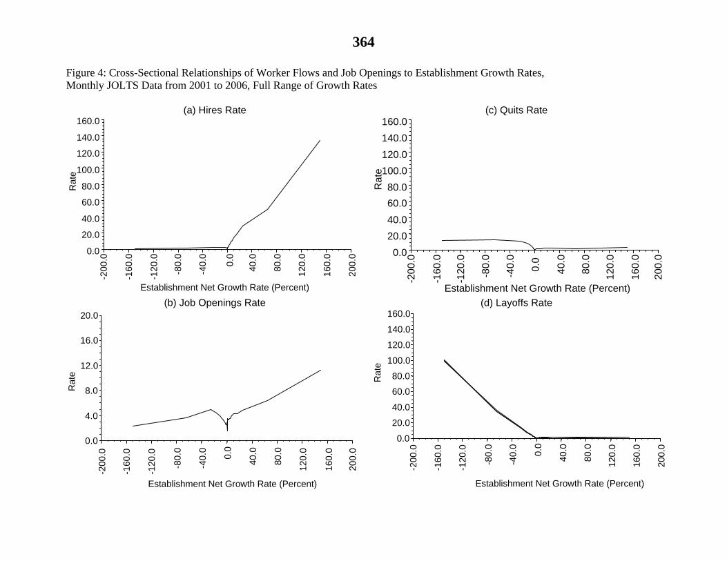
Figures 4 and 5 show how worker flows and job openings vary with employment growth
rates in the cross section of establishments. To construct these figures, we pool monthly JOLTS
data from 2001 to 2006 for private sector establishments. We group the roughly 572,000
observations into growth rate bins, calculate employment-weighted mean outcomes in each bin,
and plot the resulting relationships. We use narrow bins close to zero (width of 0.001, or 0.1
percent) and progressively wider bins as we move away from zero into thinner parts of the
distribution. We also allow for a mass point at 0. Figure 4 shows the relationships over the full
range of growth rate outcomes, and Figure 5 zooms in to monthly growth rates from -25 to 25
percent. Figure 5 also shows cross-sectional relations for the 12 months with the highest or
lowest growth rates of aggregate employment.18 The pattern for separations, not shown, is
closely approximated by the sum of quits and layoffs.19
Insert Figures 4 and 5 here
Figures 4 and 5 document several key results:
1. Hires dominate the employment adjustment margin for expanding establishments.
The hires rate is lowest for establishments with little or no growth, essentially
unrelated to growth for contracting establishments, and rises almost linearly with the
growth rate for expanding establishments.
2. Separations dominate the adjustment margin for contracting establishments. Quit,
layoff and separation rates are also lowest for establishments with little or no growth,
and they rise sharply with the contraction rate.
3. Layoffs dominate the adjustment margin for rapidly contracting establishments.
329
4. The job openings rate is lowest for stable establishments. It rises in both directions
moving away from zero, more so for expanding establishments.
5. The cross-sectional relations are remarkably stable with respect to aggregate
employment growth, especially for hires and layoffs. Conditional on establishment
growth, quits occur more frequently when aggregate employment grows more
rapidly. This cyclical aspect of quit behavior shows up mainly at contracting
establishments.
These results have important implications for JOLTS-based estimates of worker flows
and job openings.20 It is evident from Figures 4 and 5 that the overweighting of stable
establishments in the JOLTS sample imparts a downward bias in estimated hires, separations,
quits, layoffs and job openings. Less obviously, the bias is likely to vary systematically with
aggregate employment growth. To see this point, consider the layoff rate and recall our earlier
discussion of nonresponse adjustments in the JOLTS program. Suppose that nonresponse rates
are higher among rapidly contracting establishments. Because rapidly contracting
establishments are more prevalent in downturns, higher nonresponse rates among these
establishments also has a greater effect on the estimated aggregate layoff rate in downturns. In
other words, the published JOLTS statistics understate the amplitude of cyclical fluctuations in
the layoff rate.
Figure 6 confirms a key element of this cyclical bias story. As in Figure 3, Figure 6
shows smoothed histograms of quarterly establishment growth rates using JOLTS and BED data.
However, we now plot separate histograms for quarters with high and low growth in aggregate
employment. Figure 6 shows that the overweighting of stable establishments in the JOLTS
sample is more serious in downturns, i.e., quarters with low aggregate growth. The BED-JOLTS

330
difference in the 90-10 growth rate differential is 18.0 percentage points in high-growth quarters
as compared to 20.3 percentage points in low-growth quarters. Moreover, the cyclical variation
in the BED-JOLTS discrepancy is concentrated among contracting establishments: the BED-
JOLTS difference in the 50-10 growth rate differential rises from 10.5 percentage points in high-
growth quarters to 15.0 percentage points in low-growth quarters. This cyclical pattern in the
BED-JOLTS discrepancy, coupled with the cross-sectional layoff relation shown in Figures 4
and 5, implies that JOLTS understates the amplitude of aggregate layoff fluctuations.
Insert Figure 6 here
Figures 4 and 5 also suggest a constructive approach to adjusting JOLTS-based estimates
of worker flows and job openings. In particular, if we use the universe data in the BED to obtain
the distribution of establishment growth rates, we can apply the cross-sectional relationships in
Figures 4 and 5 to obtain more accurate estimates for worker flows and job openings. The next
section of the paper formalizes this idea and sets forth the details.
V. A Method for Adjusting the Published JOLTS Estimates
Partition the range of establishment growth rates into bins indexed by b, allowing for
mass points at -2 (exits), 0 (no change) and 2 (entry). Let ( )mf b be the month-m share of
employment for establishments with growth rates in bin b, and let ( )mx b denote the
employment-weighted mean rate of hires, separations, layoffs, quits or job openings for the bin.
Express the corresponding month-m aggregate rate as
(2) ( ) ( )m m mbX x b f b .
331
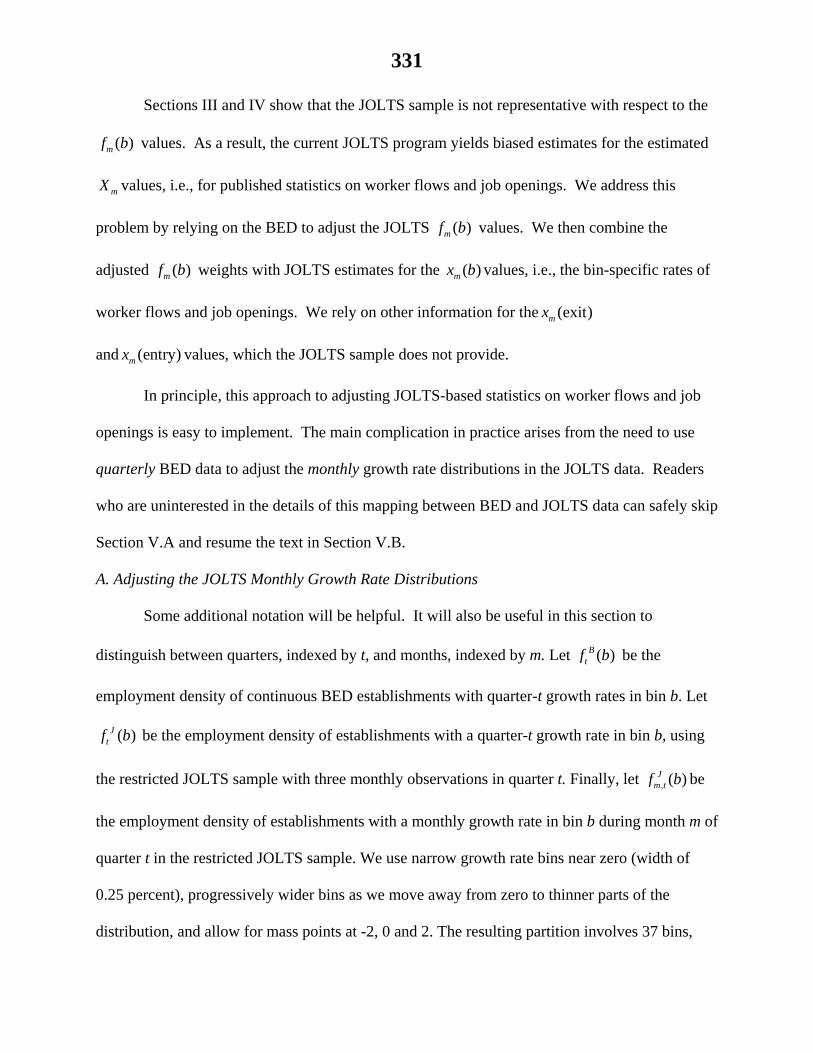
Sections III and IV show that the JOLTS sample is not representative with respect to the
( )mf b values. As a result, the current JOLTS program yields biased estimates for the estimated
mX values, i.e., for published statistics on worker flows and job openings. We address this
problem by relying on the BED to adjust the JOLTS ( )mf b values. We then combine the
adjusted ( )mf b weights with JOLTS estimates for the ( )mx b values, i.e., the bin-specific rates of
worker flows and job openings. We rely on other information for the (exit)mx
and (entry)mx values, which the JOLTS sample does not provide.
In principle, this approach to adjusting JOLTS-based statistics on worker flows and job
openings is easy to implement. The main complication in practice arises from the need to use
quarterly BED data to adjust the monthly growth rate distributions in the JOLTS data. Readers
who are uninterested in the details of this mapping between BED and JOLTS data can safely skip
Section V.A and resume the text in Section V.B.
A. Adjusting the JOLTS Monthly Growth Rate Distributions
Some additional notation will be helpful. It will also be useful in this section to
distinguish between quarters, indexed by t, and months, indexed by m. Let ( )Btf b be the
employment density of continuous BED establishments with quarter-t growth rates in bin b. Let
( )Jtf b be the employment density of establishments with a quarter-t growth rate in bin b, using
the restricted JOLTS sample with three monthly observations in quarter t. Finally, let , ( )Jm tf b be
the employment density of establishments with a monthly growth rate in bin b during month m of
quarter t in the restricted JOLTS sample. We use narrow growth rate bins near zero (width of
0.25 percent), progressively wider bins as we move away from zero to thinner parts of the
distribution, and allow for mass points at -2, 0 and 2. The resulting partition involves 37 bins,
332
although the JOLTS restricted sample and the continuous BED data contain no observations in
the entry and exit bins.
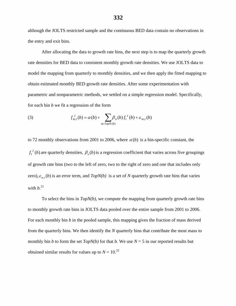
After allocating the data to growth rate bins, the next step is to map the quarterly growth
rate densities for BED data to consistent monthly growth rate densities. We use JOLTS data to
model the mapping from quarterly to monthly densities, and we then apply the fitted mapping to
obtain estimated monthly BED growth rate densities. After some experimentation with
parametric and nonparametric methods, we settled on a simple regression model. Specifically,
for each bin b we fit a regression of the form
(3)
)(
,, )()()()()(bTopNn
tmJ
tnJ
tm bbfbbbf
to 72 monthly observations from 2001 to 2006, where ( )b is a bin-specific constant, the
)(bf Jt are quarterly densities, ( )n b is a regression coefficient that varies across five groupings
of growth rate bins (two to the left of zero, two to the right of zero and one that includes only
zero), , ( )m t b is an error term, and TopN(b) is a set of N quarterly growth rate bins that varies
with b.21
To select the bins in TopN(b), we compute the mapping from quarterly growth rate bins
to monthly growth rate bins in JOLTS data pooled over the entire sample from 2001 to 2006.
For each monthly bin b in the pooled sample, this mapping gives the fraction of mass derived
from the quarterly bins. We then identify the N quarterly bins that contribute the most mass to
monthly bin b to form the set TopN(b) for that b. We use N = 5 in our reported results but
obtained similar results for values up to N = 10.22
333
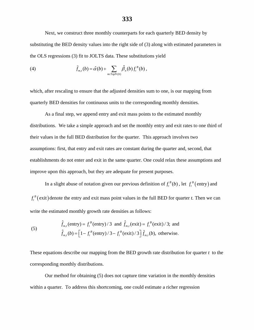
Next, we construct three monthly counterparts for each quarterly BED density by
substituting the BED density values into the right side of (3) along with estimated parameters in
the OLS regressions (3) fit to JOLTS data. These substitutions yield
(4) ,( )
ˆˆ( ) ( ) ( ) ( )Bm t n t
n TopN b
f b b b f b
,
which, after rescaling to ensure that the adjusted densities sum to one, is our mapping from
quarterly BED densities for continuous units to the corresponding monthly densities.
As a final step, we append entry and exit mass points to the estimated monthly
distributions. We take a simple approach and set the monthly entry and exit rates to one third of
their values in the full BED distribution for the quarter. This approach involves two
assumptions: first, that entry and exit rates are constant during the quarter and, second, that
establishments do not enter and exit in the same quarter. One could relax these assumptions and
improve upon this approach, but they are adequate for present purposes.
In a slight abuse of notation given our previous definition of ( )Btf b , let entryB
tf and
exitBtf denote the entry and exit mass point values in the full BED for quarter t. Then we can
write the estimated monthly growth rate densities as follows:
(5) , ,
, ,
ˆ ˆ(entry) (entry) / 3 and (exit) (exit) / 3; and
ˆ ( ) 1 (entry) / 3 (exit) / 3 ( ), otherwise.
B Bm t t m t t
B Bm t t t m t
f f f f
f b f f f b
These equations describe our mapping from the BED growth rate distribution for quarter t to the
corresponding monthly distributions.
Our method for obtaining (5) does not capture time variation in the monthly densities
within a quarter. To address this shortcoming, one could estimate a richer regression
334
specification (3) with covariates that capture within-quarter movements in the shape and location
of the aggregate employment growth rate density. This approach could be implemented with any
data source that provides monthly observations on the distribution of employment growth rates.
We leave such refinements for future work.
B. Calculating the Adjusted Estimates
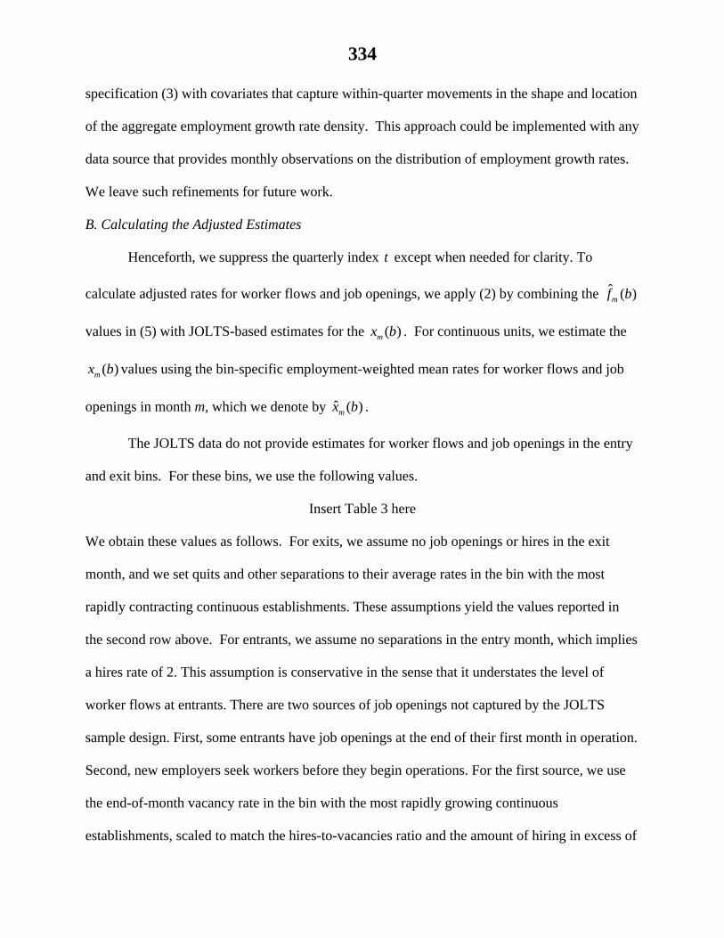
Henceforth, we suppress the quarterly index t except when needed for clarity. To
calculate adjusted rates for worker flows and job openings, we apply (2) by combining the ˆ ( )mf b
values in (5) with JOLTS-based estimates for the ( )mx b . For continuous units, we estimate the
( )mx b values using the bin-specific employment-weighted mean rates for worker flows and job
openings in month m, which we denote by ˆ ( )mx b .
The JOLTS data do not provide estimates for worker flows and job openings in the entry
and exit bins. For these bins, we use the following values.
Insert Table 3 here
We obtain these values as follows. For exits, we assume no job openings or hires in the exit
month, and we set quits and other separations to their average rates in the bin with the most
rapidly contracting continuous establishments. These assumptions yield the values reported in
the second row above. For entrants, we assume no separations in the entry month, which implies
a hires rate of 2. This assumption is conservative in the sense that it understates the level of
worker flows at entrants. There are two sources of job openings not captured by the JOLTS
sample design. First, some entrants have job openings at the end of their first month in operation.
Second, new employers seek workers before they begin operations. For the first source, we use
the end-of-month vacancy rate in the bin with the most rapidly growing continuous
establishments, scaled to match the hires-to-vacancies ratio and the amount of hiring in excess of
335
growth in the bin. This source yields a vacancy rate equal to 17.4 percent. For the second
source, we set (beginning-of-month) vacancies to the lagged vacancy rate in the bin with the
fastest-growing continuing establishments, again scaling for the hires-vacancy ratio and hiring in
excess of growth. This source yields a vacancy rate of 20.8 percent. Summing these two sources
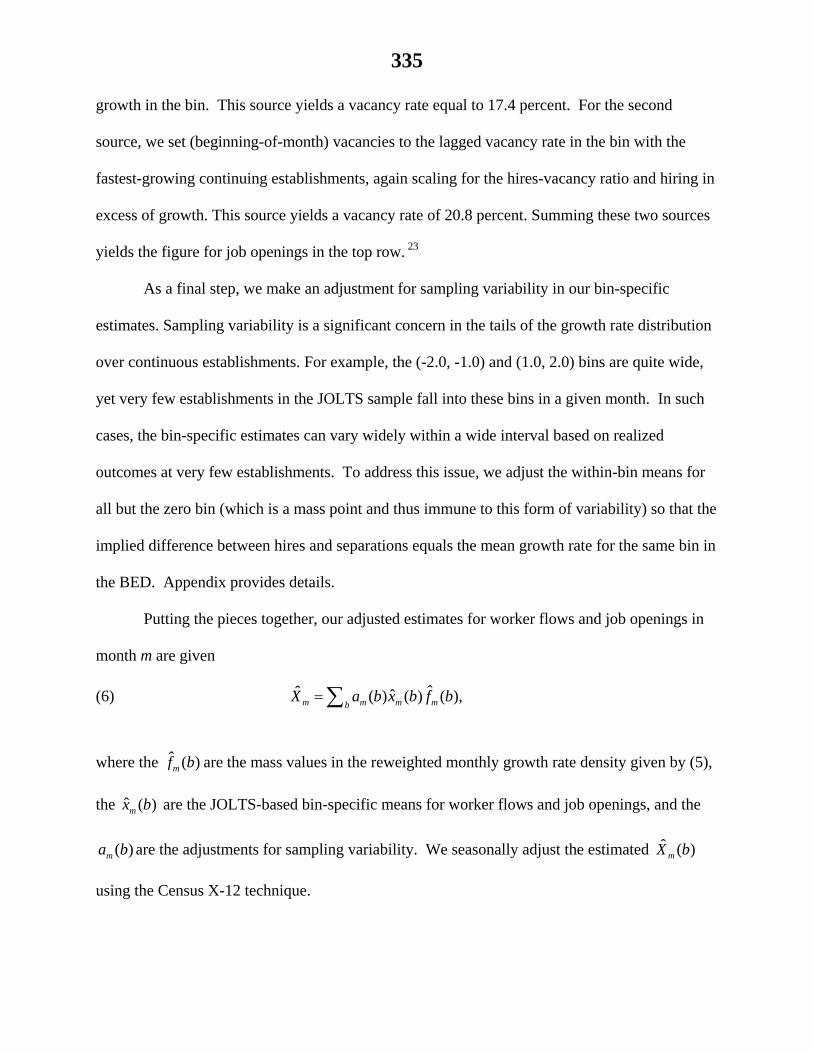
yields the figure for job openings in the top row. 23
As a final step, we make an adjustment for sampling variability in our bin-specific
estimates. Sampling variability is a significant concern in the tails of the growth rate distribution
over continuous establishments. For example, the (-2.0, -1.0) and (1.0, 2.0) bins are quite wide,
yet very few establishments in the JOLTS sample fall into these bins in a given month. In such
cases, the bin-specific estimates can vary widely within a wide interval based on realized
outcomes at very few establishments. To address this issue, we adjust the within-bin means for
all but the zero bin (which is a mass point and thus immune to this form of variability) so that the
implied difference between hires and separations equals the mean growth rate for the same bin in
the BED. Appendix provides details.
Putting the pieces together, our adjusted estimates for worker flows and job openings in
month m are given
(6) ˆˆ ˆ( ) ( ) ( ),m m m mbX a b x b f b
where the ˆ ( )mf b are the mass values in the reweighted monthly growth rate density given by (5),
the ˆ ( )mx b are the JOLTS-based bin-specific means for worker flows and job openings, and the
( )ma b are the adjustments for sampling variability. We seasonally adjust the estimated ˆ ( )mX b
using the Census X-12 technique.
336
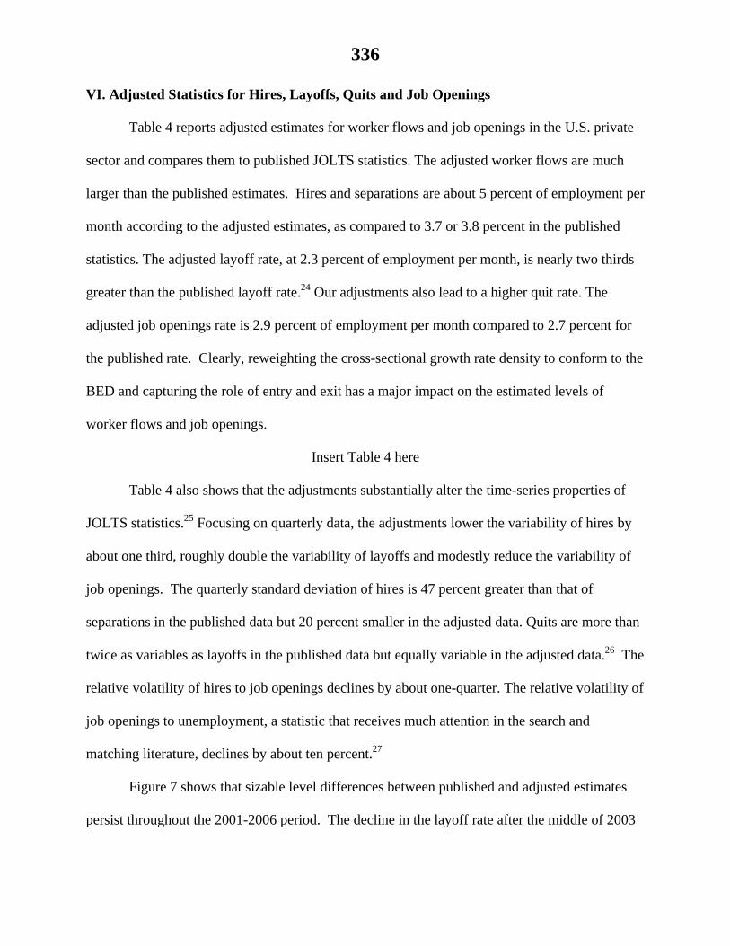
VI. Adjusted Statistics for Hires, Layoffs, Quits and Job Openings
Table 4 reports adjusted estimates for worker flows and job openings in the U.S. private
sector and compares them to published JOLTS statistics. The adjusted worker flows are much
larger than the published estimates. Hires and separations are about 5 percent of employment per
month according to the adjusted estimates, as compared to 3.7 or 3.8 percent in the published
statistics. The adjusted layoff rate, at 2.3 percent of employment per month, is nearly two thirds
greater than the published layoff rate.24 Our adjustments also lead to a higher quit rate. The
adjusted job openings rate is 2.9 percent of employment per month compared to 2.7 percent for
the published rate. Clearly, reweighting the cross-sectional growth rate density to conform to the
BED and capturing the role of entry and exit has a major impact on the estimated levels of
worker flows and job openings.
Insert Table 4 here
Table 4 also shows that the adjustments substantially alter the time-series properties of
JOLTS statistics.25 Focusing on quarterly data, the adjustments lower the variability of hires by
about one third, roughly double the variability of layoffs and modestly reduce the variability of
job openings. The quarterly standard deviation of hires is 47 percent greater than that of
separations in the published data but 20 percent smaller in the adjusted data. Quits are more than
twice as variables as layoffs in the published data but equally variable in the adjusted data.26 The
relative volatility of hires to job openings declines by about one-quarter. The relative volatility of
job openings to unemployment, a statistic that receives much attention in the search and
matching literature, declines by about ten percent.27
Figure 7 shows that sizable level differences between published and adjusted estimates
persist throughout the 2001-2006 period. The decline in the layoff rate after the middle of 2003

337
is noticeably larger in the adjusted data. Figure 8 shows that adjusted quits exceed layoffs in the
relatively strong labor market of 2005 and 2006 but are otherwise very similar in magnitude.
Insert Figures 7 and 8 here
As we remarked above, the cumulative employment growth implied by the flow of hires
and separations in JOLTS exceeds employment growth in the Current Establishment Statistics
and the BED. Our adjustments largely eliminate this discrepancy. The published JOLTS
statistics imply an average monthly growth rate of 0.08 percent for private sector employment.
The corresponding growth rate in the CES is about 0.04 percent and the monthly analog of the
BED growth rate is 0.03 percent. Our adjusted estimates imply a mean growth rate of 0.03
percent. This is in line with the monthly BED growth rate, the appropriate comparison since it is
the rate our adjustment is constructed to reproduce. It is also quite close to the CES growth rate.
VII. Concluding Remarks
JOLTS data are a valuable resource for understanding labor market dynamics and for
evaluating theories of unemployment and worker turnover. They also present measurement
issues that are not well understood or fully appreciated. A key point is that the JOLTS sample
overweights relatively stable establishments with low rates of hires and separations, and
underweights establishments with rapid growth or contraction. The unrepresentative nature of
the JOLTS sample with respect to the cross-sectional density of employment growth rates
matters because hires, quits, layoffs and job openings vary greatly with establishment growth
rates in the cross section. As a result, the current JOLTS program produces downwardly biased
estimates for worker flows and job openings. The extent of bias varies systematically with the
growth rate of aggregate employment.

338
We develop and implement an adjustment method to address these issues. Our method
reweights the cross-sectional density of employment growth rates in JOLTS to match the
corresponding density in comprehensive BED data. In addition, our method supplements JOLTS
data on worker flows and job openings at continuing establishments with estimates for worker
flows and job openings at entering and exiting establishments. Our adjustments have a large
effect on JOLTS-based estimates. Adjusted hires and separations exceed the published statistics
by about one-third. Layoffs are much larger and much more variable in the adjusted statistics,
and they account for a bigger share of separations.
There are several steps that the BLS can undertake to improve the JOLTS sample and
JOLTS-based statistics. First, as part of a regular program to monitor the JOLTS sample, the
BLS should compare the cross-sectional densities of employment growth rates in JOLTS data to
the corresponding densities in the BED or other comprehensive source. Because of lags in the
availability of administrative records that feed into the BED, it is not feasible to reweight the
JOLTS density to conform to the BED as part of a real-time monthly production process. It is
feasible to reweight the JOLTS density to conform to the growth rate distribution in the monthly
CES, as adjusted for systematic differences between the CES and comprehensive sources in
historical data.
Second, the BLS should explicitly incorporate adjustments for worker flows and job
openings at establishments that are outside the JOLTS sample frame. The BLS already models
the effects of entry and exit in its CES employment estimates. Adapting and extending BLS
models to capture the effects of entry and exit on hires, separations and job openings is entirely
feasible using information available from JOLTS, BED and CES data. It would also be useful to
conduct special surveys with retrospective questions about worker flows and job openings at new
339
establishments, including questions about the number job openings before an entrant began
operations. Information obtained from this type of survey would provide a strong basis for
imputing worker flows and job openings to new establishments as part of a monthly production
process.
Third, the BLS should investigate the potential payoff from sample stratification on
establishment age and from corrections for the exclusion of very young establishments from the
JOLTS sample frame. As discussed in the introduction, young establishments have unusually
high worker flows, even after conditioning on establishment size. Our adjustment method does
not directly address this source of downward bias in JOLTS-based estimates for hires and
separations.28 We suspect that very limited sample stratification on establishment age and simple
corrections for the exclusion of very young establishments would go a long ways to address this
source of bias, because hires and separations decline very rapidly with establishment age initially
but then flatten out. Here as well, special surveys could provide a reliable basis for imputing
worker flows and job openings to young establishments that are underweighted or excluded from
the JOLTS sample frame.
Fourth, the BLS should carefully investigate how the unit nonresponse rate varies with
the establishment growth rate in the JOLTS sample. In this regard, it is essential to evaluate the
nonresponse rate throughout the entire distribution of growth rates. Suppose, for example, that
the response rate is very high on average but is smaller in certain parts of the growth rate
distribution. This type of nonresponse pattern leads to biased estimates for aggregate worker
flows and job openings because these measures vary greatly with establishment growth rates in
the cross section. Determining whether, and how, the unit nonresponse rate varies with the
establishment growth rate is a straightforward exercise. It can be carried out by matching JOLTS
340
micro data to data from the BED or other comprehensive source and then directly computing
nonresponse rates as a function of the establishment growth rate. Having obtained this function,
it would be a simple matter to adjust JOLTS-based estimates of worker flows and job openings
for unit nonresponse rates that vary with the establishment growth rate.
Another potential issue in JOLTS data is respondent error – the propensity of
establishments to misreport their true number of hires, separations or job openings to the BLS.
Wohlford et al. (2003) and Faberman (2005a) express concerns about respondent error as a
source of bias in JOLTS-based statistics. The methods we develop in this paper do not address
respondent error. Thus, this paper should be viewed as part of a broader effort to better
understand and improve JOLTS-based statistics.
While measurement issues are our main focus in this paper, our findings have
implications for the broader study of labor market dynamics. In this regard, some authors have
interpreted data on the relative volatility of separations and hires as favoring a hires-driven view
of recession (Hall, 2005; Shimer, 2007a). We find that using a representative growth rate
distribution to estimate worker flows substantially increases the variability of separations relative
to hires – so much so that separations are more variable than hires according to our adjusted
estimates.
The adjustment method we introduce in this paper is potentially useful in other settings as
well, and these settings are relatively easy to identify. In particular, when the outcome measure
of interest varies with micro growth rates in the cross section, it is important to evaluate whether
the sample produces a representative cross-sectional growth rate distribution. If the sample is
not representative in this respect, and if the outcome variable varies systematically with growth
rates in the cross section, then sample means of the outcome variable are biased. That is the

341
essence of the problem in the JOLTS sample that we consider in this paper. Analogous problems
potentially arise in surveys of capital investment and disinvestment, because investment
outcomes differ systematically between declining and growing businesses.
Finally, we note that our adjustment method can be applied to “backcast” worker flows
and job openings before the period covered by the JOLTS sample. In particular, one could
combine historical data on the cross-sectional distribution of establishment growth rates from the
CES, BED or other source with JOLTS-based data on the cross-sectional relations displayed in
Figures 4 and 5 to construct historical time series for worker flows and job openings. Such an
endeavor would greatly expand the time-series dimension of data available for the study of labor
market dynamics.
342
Endnotes
1 See Wohlford et al. (2003), Nagypál (2006) and Faberman (2005a).
2 See Faberman (2005a) and Davis, Faberman and Haltiwanger (2006).
3 See Faberman (2005a).
4 See, for example, Mincer and Jovanovic (1981), Topel and Ward (1992), and Farber (1994).
5 See Davis and Haltiwanger (1999) and Davis et al. (2007).
6 In early 2009, following the conclusion of this research project, the BLS made substantial revisions to
the published JOLTS statistics. The revisions reflected several of our suggestions, and consequently
resolve some of the issues noted below. For example, the revised JOLTS statistics now have net growth
rates that are generally consistent with those derived from the CES. Revised worker flow rates are also
higher, on average, though still below the magnitudes of the adjusted estimates in this chapter. The full
details of the BLS revisions can be found at http://www.bls.gov/jlt/methodologyimprovement.htm. This
study uses published and micro data prior to the revisions.
7 For evidence, see Davis, Faberman and Haltiwanger (2006, 2007) and Section III below.
8 See Clark and Hyson (2001) and Faberman (2005b) for information about the JOLTS program and
Spletzer et al. (2004) for more information about the BED. Statistics derived from the JOLTS program
are available at http://www.bls.gov/jlt/home.htm.
9 The JOLTS survey form instructs the respondent to report a job opening when “A specific position
exists, work could start within 30 days, and [the establishment is] actively seeking workers from outside
this location to fill the position.” Further instructions define “active recruiting” as “taking steps to fill a
position … [that] may include advertising in newspapers, on television, or on radio; posting Internet
notices; posting ‘help wanted’ signs; networking or making ‘word of mouth’ announcements; accepting
applications; interviewing candidates; contacting employment agencies; or soliciting employees at job
fairs, state or local employment offices, or similar sources.” Job openings are not to include positions

343
open only to internal transfers, promotions, recalls from temporary layoffs, or positions to be filled by
temporary help agencies, outside contractors, or consultants.
10 Independent contractors and unincorporated self-employed persons are out of scope for the QCEW,
making them out of scope for the JOLTS, CES and BED as well.
11 Our discussion in the text ignores outlier adjustments, sample rotation, and item nonresponse (as
distinct from unit nonresponse). For more on the JOLTS estimation methodology, see Crankshaw and
Stamas (2000).
12 In general, a sample that is representative with respect to levels, such as employment, need not be
representative with respect to changes, such as employment growth rates. Worker flows and job openings
are much more closely related to employment changes than employment levels. Hence, the
benchmarking and nonresponse adjustments that constrain JOLTS employment totals to match sample
frame employment do not ensure unbiased estimates of worker flows and job openings. See the recent
National Academy of Sciences report by Haltiwanger et al. (2007) for additional discussion of the
distinction between samples optimized for levels and samples optimized for changes.
13 Available at http://www.bls.gov/bdm/.
14 See Davis, Haltiwanger and Schuh (1996) for more on this growth measure. The BED program uses
this growth rate measure in its published statistics for gross job gains and losses.
15 Wohlford et al. (2003) point to education (mostly in State and Local Government) and temporary help
(part of Professional and Business Services) as the main sources of the JOLTS-CES divergence. Using
published JOLTS data, we confirm that the employment path implied by JOLTS hires and separations
exhibits an especially large divergence from the CES employment path in Professional and Business
Services. The cumulative discrepancy for this industry group is 3.6 million jobs, or 20.5 percent of the
industry’s December 2006 CES employment value. Education, Health, and Leisure and Hospitality also
exhibit large cumulative discrepancies in the same direction. There are large cumulative discrepancies in
the opposite direction in Construction (1.1 million jobs, 14.8 percent of employment) and Manufacturing

344
(1.1 million jobs, 7.5 percent of employment). In short, several major industry groups show big
cumulative discrepancies over the 2001 to 2006 period.
16 Recall that we construct internally consistent measures of lagged employment using current-quarter
JOLTS data for hires, separations and employment. In particular, if an establishment has employees in all
three months of the current quarter, we calculate its growth rate using reported employment for the
current quarter and the internally consistent measure of previous quarter employment. Thus, the restricted
JOLTS sample captures establishments that operate continuously from the last month of the previous
quarter to the last month of the current quarter. The JOLTS sample restriction removes 11.2 percent of
the observations on a sample-weighted basis and a much smaller percentage when we further weight by
size.
17 The overweighting of stable establishments in Figure 3 and Table 2 is not caused by our use of hires
and separations to measure previous-period employment when calculating JOLTS-based measures of the
employment growth rate. This point can be seen by inspecting Figure 5 in Faberman (2005a), which
shows that the employment-weighted growth rate distribution in the JOLTS sample is extremely similar
whether we compute growth rates using the reported value of lagged employment or the imputed value
based on the identity linking employment changes to hires and separations. Figure 5 in Faberman also
shows that the JOLTS sample substantially overweights stable establishments relative to the BED for
both approaches to the calculation of employment growth rates in the JOLTS sample.
18 When ranking the months by aggregate growth rates, we do not seasonally adjust the data. The
unadjusted data have much larger variations in growth over time, so are better suited for this exercise.
19 The other separations rate (not shown) rises with the contraction rate from about 0.3 percent of
employment per month for mild contractions to 7.4 percent for the largest contractions.
20 In related work (Davis, Faberman and Haltiwanger, 2006), we argue that the cross-sectional relations in
Figures 4 and 5 also have important implications for the cyclical behavior of unemployment.
345
21 Allowing the coefficients to vary by individual growth rate bin yields noisy estimates because of
sparsely populated bins, particularly at the tails of the growth rate distribution. After some
experimentation, we set the boundary for the two bins to the left and to the right of zero at 9 percent.
22 The choice of N has little effect on the magnitude or time-series volatility of our adjusted worker flow
rates and vacancy rates. However, alternative choices of N imply different paths for cumulative
employment growth over the six-year sample period. The choice of N = 5 minimizes the absolute
difference of cumulative employment growth between the adjusted JOLTS figures and the BED.
23 This discussion suggests that the JOLTS program would benefit from retrospective questions about pre-
entry job openings for new establishments. A similar point applies to other establishment surveys that
seek to capture activities that are correlated with entry. For example, it would be helpful to add
retrospective questions about initial investments for entrants in the Annual Capital Expenditures Survey.
24 To understand the large upward adjustment in the layoff rate, recall that layoffs are disproportionately
concentrated in establishments that exit or contract sharply (Figures 4 and 5). These establishments are
heavily underweighted in the JOLTS sample, as documented in Table 2.
25 Given the limitations of our data and methods, we think our adjustments produce more reliable
evidence for quarterly than for monthly fluctuations. For this reason, Table 3 reports standard deviations
of monthly and quarterly values, and the lower panel focuses on volatility statistics in quarterly data.
However, the upper panel suggests that the choice between quarterly and monthly data matters little in
this regard.
26 A careful inspection of Figure 5 suggests that the impact of our adjustments on the relative volatility of
hires and separations, or quits and layoffs, would be somewhat smaller if we extended the regression
specification (3) to capture time variation in the cross-sectional relations.
27 For example, see Shimer (2005), Gertler and Trigari (2005), and Hagedorn and Manovskii (2007).

346
28 Our adjustment method relies on JOLTS data to provide unbiased estimates for ˆ( )x b in equation (6).
However, the underweighting of younger establishments in JOLTS data imparts a downward bias to the
ˆ( )x b estimates.
347
References
Clark, Kelly A., and Hyson, Rosemary, 2001. “New Tools for Labor Market Analysis: JOLTS.”
Monthly Labor Review, 124(12): 32-37.
Crankshaw, Mark and George Stamas (2000) “Sample Design in the Job Openings and Labor
Turnover Survey,” 2000 Proceedings of the Annual Statistical Association [CD-ROM].
Alexandria, VA: American Statistical Association.
Davis, Steven J., Faberman, R. Jason, and Haltiwanger, John, 2006. “The Flow Approach to
Labor Markets: New Evidence and Micro-Macro Links.” Journal of Economic Perspectives,
20(3): 3-24.
Davis, Steven J., Faberman, R. Jason, and Haltiwanger, John C., 2007. “The Establishment-
Level Behavior of Vacancies and Hiring,” mimeo.
Davis, Steven J. and John Haltiwanger (1999) “Gross Job Flows,” Handbook of Labor
Economics, Volume 3B, Orley Ashenfelter and David Card, editors, Amsterdam: North-Holland.
Davis, Steven, John Haltiwanger, Ron Jarmin, C.J. Krizan, Javier Miranda, Alfred Nucci and
Kristin Sandusky (2007), NBER Working Paper No. 13226. Forthcoming in Producer
Dynamics: New Evidence from Micro Data, edited by Timothy Dunne, J. Bradford Jensen and
Mark J. Roberts.
348
Davis, Steven J., John C. Haltiwanger, and Scott Schuh, Job Creation and Destruction
(Cambridge, MA: MIT Press, 1996).
Faberman, R. Jason, 2005a. “Analyzing the JOLTS Hires and Separations Data.” 2005
Proceedings of the Annual Statistical Association [CD-ROM]. Alexandria, VA: American
Statistical Association.
Faberman, R. Jason, 2005b. “Studying the Labor Market with the Job Openings and Labor
Turnover Survey.” Bureau of Labor Statistics Working Paper No. 388. Forthcoming in Producer
Dynamics: New Evidence from Micro Data, edited by Timothy Dunne, J. Bradford Jensen and
Mark J. Roberts.
Faberman, R. Jason, 2006. “Job Flows and the Recent Business Cycle: Not All ‘Recoveries’ Are
Created Equal,” BLS Working Paper No. 391.
Faberman, R. Jason, and Éva Nagypál, 2007. “The Effect of Quits on Worker Recruitment:
Theory and Evidence,” mimeo.
Fallick, Bruce and Charles A. Fleischman, 2004. “Employer-to-Employer Flows in the U.S.
Labor Market: The Complete Picture of Gross Worker Flows,” Federal Reserve Board of
Governors, Finance and Economics Discussion Series Paper No. 2004-34.

349
Farber, Henry S. (1994) “The Analysis of Interfirm Worker Mobility,” Journal of Labor
Economics, 12, no. 4 (October), 554-593.
Fujita, Shigeru, and Gary Ramey, 2007. “Job Matching and Propagation,” forthcoming, Journal
of Economic Dynamics and Control.
Gertler, Mark and Antonella Trigari, 2005. “Unemployment Fluctuations with Staggered
Nash Bargaining,” mimeo, New York University.
Hagedorn, Marcus and Iourii Manovskii, 2007. “The Cyclical Behavior of Equilibrium
Unemployment and Vacancies Revisited,” mimeo, University of Pennsylvania.
Hall, Robert E., 2005. “Job Loss, Job Finding, and Unemployment in the U.S. Economy over the
Past Fifty Years,” forthcoming, 2005 NBER Macroeconomics Annual, Cambridge, MA: MIT
Press.
Haltiwanger, John, Lisa Lynch and Chris Mackie (eds.), 2007. Understanding Business
Dynamics: An Integrated Data System for America's Future, Washington, DC: National
Academies Press.
Mincer, Jacob and Boyan Jovanovic (1981) “Labor Mobility and Wages,” in Studies in Labor
Markets, edited by Sherwin Rosen. Chicago: University of Chicago Press.
350
Mortensen, Dale T., and Pissarides, Christopher A., 1994. “Job Creation and Job Destruction and
the Theory of Unemployment.” Review of Economic Studies 61(3): 397-415.
Nagypál, Éva, 2006. “What Can We Learn About Firm Recruitment from the Job Openings and
Labor Turnover Survey?” forthcoming, Producer Dynamics: New Evidence from Micro Data
(Timothy Dunne, J. Bradford Jensen, and Mark J. Roberts, editors), University of Chicago Press.
Shimer, Robert, 2005. “The Cyclical Behavior of Equilibrium Unemployment and Vacancies,”
American Economic Review 95(1): 25-49.
Shimer, Robert, 2007a. “Reassessing the Ins and Outs of Unemployment.” University of
Chicago: mimeo.
Shimer, Robert, 2007b. “Mismatch,” American Economic Review, 97(4): 1074-1101.
Spletzer, James R.; Faberman, R. Jason; Sadeghi, Akbar; Talan, David M. and Clayton, Richard
L., 2004. “Business Employment Dynamics: New Data on Gross Job Gains and Losses,”
Monthly Labor Review, 127(4), pp. 29-42.
Topel, Robert H. and Michael P. Ward (1992) “Job Mobility and the Careers of Young Men,”
Quarterly Journal of Economics, 107, no. 2 (May), 439-479.
351
Valetta, Robert, 2005. “Why has the U.S. Beveridge Curve Shifted Back? New Evidence Using
Regional Data,” Federal Reserve Bank of San Francisco Working Paper No. 2005-25.
Wohlford, John, Phillips, Mary Anne, Clayton, Richard, and Werking, George, 2003.
“Reconciling labor turnover and employment statistics.” 2003 Proceedings of the Annual
Statistical Association [CD-ROM]. Alexandria, VA: American Statistical Association.

352
Appendix
A. Calculating Quarterly Flows and Growth Rates
In comparing JOLTS and BED data in Table 2 and Figures 3 and 6, we need a consistent
measure of quarterly growth rates. There is an issue of how to measure quarterly growth rates in
the JOLTS data because JOLTS sample weights change from month to month. To deal with this
issue, we measure quarterly flows as the sum of weighted monthly values divided by the weight
for the last month in the quarter:
tm
tmtmtmtmtmtmt
xxxx
,
,2,2,1,1,,
,
where tx is the quarterly rate for quarter t, ,m tx is the monthly rate for month m in quarter t, ,m t
is the weight for month m in quarter t, and we have suppressed the index for establishments.
When computing the internally consistent measure of lagged quarterly employment analogous to
equation (1) in the main text, we use the level of employment in the last month of the quarter
together with the quarterly measures of hires and separations defined above.
B. Adjusting the bin-specific estimates for sampling variability
The sampling-variability adjustment factor for the estimate ,ˆ ( )m tx b is given by
, , ,( ) ( ) ( ) ( )Bm t t m t m ta b n b h b s b ,
where ( )Btn b is the mean net growth rate for bin b in quarter t in the BED data, and h and s
denote rates of hires and separations, respectively in the JOLTS data. This adjustment factor
constrains the resulting mean net growth rate in bin b in the adjusted JOLTS data to equal the
mean net growth rate in the corresponding bin in the BED data. It would be better to impose this

353
constraint using CES rather than BED data; however, the CES micro data were not available to
us for this project.
354
Table 1: Average Monthly Worker Flows as a Percent of Employment, 2001-2006 Hires Rate Separations Rate
JOLTS, Published Statistics 3.4 3.3
CPS Gross Flows, Fallick-Fleischman 6.4 6.4
Note: Table entries report mean monthly rates for hires and separations from January 2001 to
December 2006. The statistics on CPS gross flows are from Fallick and Fleischmann (2004), as
updated at http://www.federalreserve.gov/pubs/feds/2004/200434/200434abs.html. CPS hires
and separations include employment-to-employment flows.
355
Table 2: Cross-Sectional Growth Rate Distributions, 2001 to 2006
JOLTS BED
Growth Rate Interval
Monthly, Full
Sample
Monthly, Restricted
Sample
Quarterly, Restricted
Sample
Quarterly, All
Observations
Quarterly, Continuous
Observations-2.0 (exits) --- --- --- 0.7 ---
(-2.0, -0.20] 1.6 1.5 4.3 7.5 7.6
(-0.20, -0.05] 7.1 7.0 13.2 16.5 16.7
(-0.05, -0.02] 7.9 7.8 9.5 9.6 9.7
(-0.02, 0.0) 14.7 14.6 11.6 7.6 7.8
0.0 33.6 34.1 17.1 15.4 15.7
(0.0, 0.02) 16.5 16.6 13.1 7.9 8.0
[0.02, 0.05) 9.2 9.1 11.7 9.9 10.0
[0.05, 0.20) 7.9 7.8 15.1 16.7 16.9
[0.20, 2.0) 1.6 1.5 4.5 7.5 7.6
2.0 (entrants) --- --- --- 0.7 ---
Note: Table entries report employment shares for the indicated establishment growth rate
intervals in JOLTS and BED micro data from 2001 to 2006. Calculations on JOLTS data make
use of the JOLTS final sample weights described in Section II.A. Each column in the table
reports results for a different data set or sample. See the text for a detailed explanation of how
the data sets and samples differ.

356
Table 3: Rates for Entry and Exit Bins
Bin Hires Quits LayoffsOther
SeparationsJob
Openingsb = entry 2 0 0 0 0.382
b = exit 0 0.124 1.802 0.074 0
357
Table 4: JOLTS Summary Statistics, Published and Adjusted Statistics Published Statistics Adjusted Statistics Means (Monthly, Quarterly Standard Deviations)
Hires Rate (H) 3.78
(0.25, 0.23)
4.99
(0.17, 0.16)
Separations Rate (S) 3.70
(0.18, 0.16)
4.96
(0.21, 0.20)
Quits Rate (Q) 2.06
(0.17, 0.17)
2.36
(0.17, 0.15)
Layoffs and Discharges Rate (L) 1.40
(0.09, 0.07)
2.29
(0.16, 0.15)
Other Separations Rate (R) 0.24
(0.03, 0.02)
0.31
(0.07, 0.05)
Job Openings Rate (V) 2.71
(0.39, 0.38)
2.94
(0.36, 0.34)
Unemployment Rate (U) 5.29
(0.57, 0.58) ---
Quarterly Relative Volatilities
(H)/ (S) 1.47 0.80
(Q)/ (L) 2.35 1.00
(H)/ (V) 0.61 0.47
(V)/ (U) 0.66 0.59 Notes: Table lists the noted monthly statistics from the publicly available JOLTS estimates and
the adjusted estimates (see text for details). Standard deviations of the monthly data, followed by
the quarterly means of the monthly data (or third-month values in the case of the vacancy and
unemployment rate), are in parentheses below each mean. Relative volatilities are the ratios of
the quarterly standard deviations of the listed estimates. The period covers January 2001 –
December 2006. The unemployment rate comes from the Current Population Survey.

358
Chapter 5: Steven J. Davis et al.
Figure 1: CES and JOLTS Employment Growth Rates Compared
Notes: Figure depicts the quarterly net employment growth rates calculated from the JOLTS and
CES data. The JOLTS growth rate is measured from the difference in total hires and total
separations for each quarter. The CES growth rate is measured from the net change in
employment levels between the third month of each quarter. Both rates are calculated using the
average of the current and previous quarter’s employment in the denominator.
Figure 2: CES Employment Path Compared to Cumulated Differences between Hires and
Separations in JOLTS
Notes: Figure depicts the employment levels implied from the JOLTS hires and separations data
and reported in the CES data. The JOLTS level is reported two ways: as an accumulation of the
difference between hires and separations each month (added to the December 2000 total) and as
the accumulation over each year of the survey, added to the beginning-of-year employment level
Figure 3: Cross-Sectional Densities for Establishment Growth Rates, 2001-2006
Notes: The densities are constructed as smoothed histograms of quarterly employment growth
rates using establishment-level observations in JOLTS (restricted sample) and BED (all
observations) from 2001Q1 to 2006Q4. Histograms are constructed over the full growth rate
distribution, but the figure zooms in on growth rates from -25 to 25 percent per quarter.
Histogram bins are narrower for smaller growth rates and allow for mass points at growth rates
of -2.0 (exit), 0 (no change) and 2.0 (entry).
359
Figure 4: Cross-Sectional Relationships of Worker Flows and Job Openings to Establishment
Growth Rates, Monthly JOLTS Data from 2001 to 2006, Full Range of Growth Rates
Figure 5: Cross-Sectional Relationships of Worker Flows and Job Openings to Establishment
Growth Rates, Monthly JOLTS Data from 2001 to 2006, Zoomed in on Growth Rates from -25
and 25 Percent
Notes: Thick lines are constructed from the full 2001-2006 sample. Thin lines are constructed
from samples restricted to the 12 months with the highest or lowest growth rate of aggregate
employment. The upper thin lines typically correspond to the high-growth sample.
Figure 6: Quarterly Growth Rate Distributions in High- and Low-Growth Quarters, JOLTS and
BED Data
Notes: Figures depict employment densities at establishments with quarterly growth rates within
a given interval in the BED (top panel) and a restricted panel of JOLTS data (bottom panel, see
text for details of restriction) for 2001Q1 – 2006Q4. The distributions are split into the 6 quarters
of highest growth and 6 quarters of lowest growth, based on their seasonally unadjusted
aggregate growth rates in the BED. Vertical lines represent the growth rates at the 10th (shaded
lines) and 90th (dashed lines) percentiles of the distribution, with the leftmost of each pair
associated with each low-growth distribution.

360
Figure 7: Adjusted and Published Estimates of JOLTS Worker Flows and Job Openings
Notes: Each panel illustrates a worker flow or job openings rate, seasonally adjusted, from the
published JOLTS statistics (dashed line) and our adjusted estimates (solid line). See text for
details of the adjustment.
Figure 8: Adjusted Quit and Layoff Rates, JOLTS Data
Notes: The figure illustrates the quit rate and layoff rate, seasonally adjusted, from our adjusted
estimates. See text for details of the adjustment.

361
Figure 1: CES and JOLTS Employment Growth Rates Compared
Notes: Figure depicts the quarterly net employment growth rates calculated from the JOLTS and
CES data. The JOLTS growth rate is measured from the difference in total hires and total
separations for each quarter. The CES growth rate is measured from the net change in
employment levels between the third month of each quarter. Both rates are calculated using the
average of the current and previous quarter’s employment in the denominator.
-0.8
-0.6
-0.4
-0.2
0.0
0.2
0.4
0.6
0.8
1.0
1.2
Dec
-200
0
Ma r
-200
1
Jun-
2001
Sep
-200
1
Dec
-200
1
Ma r
-200
2
Jun-
2002
Sep
-200
2
Dec
-200
2
Mar
-200
3
Jun-
2003
Sep
-200
3
Dec
-200
3
Ma r
-200
4
Jun-
2004
Sep
-200
4
Dec
-200
4
Mar
-200
5
Jun-
2005
Sep
-200
5
Dec
-200
5
Mar
-200
6
Jun-
2006
Sep
-200
6
Dec
-200
6
Per
cent
of E
mpl
oym
ent
CES Net Growth Rate JOLTS Net Growth Rate
362
Figure 2: CES Employment Path Compared to Cumulated Differences between Hires and Separations in JOLTS
Notes: Figure depicts the employment levels implied from the JOLTS hires and separations data
and reported in the CES data. The JOLTS level is reported two ways: as an accumulation of the
difference between hires and separations each month (added to the December 2000 total) and as
the accumulation over each year of the survey, added to the beginning-of-year employment level.
128.0
130.0
132.0
134.0
136.0
138.0
140.0
142.0
144.0
Dec
-200
0
Ma r
-200
1
Jun-
2001
Sep
-200
1
Dec
-200
1
Ma r
-200
2
Jun-
2002
Sep
-200
2
Dec
-200
2
Ma r
-200
3
Jun-
2003
Sep
-200
3
Dec
-200
3
Ma r
-200
4
Jun-
2004
Sep
-200
4
Dec
-200
4
Mar
-200
5
Jun-
2005
Sep
-200
5
Dec
-200
5
Ma r
-200
6
Jun-
2006
Sep
-200
6
Dec
-200
6
Em
ploy
men
t (0
00s)
Cumulative JOLTS Implied Employment
Employment Implied by JOLTS Hires - Separations
CES Employment
363
Figure 3: Cross-Sectional Densities for Establishment Growth Rates, 2001-2006
Notes: The densities are constructed as smoothed histograms of quarterly employment growth
rates using establishment-level observations in JOLTS (restricted sample) and BED (all
observations) from 2001Q1 to 2006Q4. Histograms are constructed over the full growth rate
distribution, but the figure zooms in on growth rates from -25 to 25 percent per quarter.
Histogram bins are narrower for smaller growth rates and allow for mass points at growth rates
of -2.0 (exit), 0 (no change) and 2.0 (entry).
364
Figure 4: Cross-Sectional Relationships of Worker Flows and Job Openings to Establishment Growth Rates, Monthly JOLTS Data from 2001 to 2006, Full Range of Growth Rates
(a) Hires Rate
(b) Job Openings Rate
(c) Quits Rate
(d) Layoffs Rate
0.0
20.0
40.0
60.0
80.0
100.0
120.0
140.0
160.0
-200
.0
-160
.0
-120
.0
-80.
0
-40.
0
0.0
40.0
80.0
120.
0
160.
0
200.
0
Establishment Net Growth Rate (Percent)
Rat
e
0.0
20.0
40.0
60.0
80.0
100.0
120.0
140.0
160.0
-200
.0
-160
.0
-120
.0
-80.
0
-40.
0
0.0
40.0
80.0
120.
0
160.
0
200.
0
Establishment Net Growth Rate (Percent)
Rat
e
0.0
4.0
8.0
12.0
16.0
20.0
-200
.0
-160
.0
-120
.0
-80.
0
-40.
0
0.0
40.0
80.0
120.
0
160.
0
200.
0
Rat
e
Establishment Net Growth Rate (Percent)
0.0
20.0
40.0
60.0
80.0
100.0
120.0
140.0
160.0
-200
.0
-160
.0
-120
.0
-80.
0
-40.
0
0.0
40.0
80.0
120.
0
160.
0
200.
0
Establishment Net Growth Rate (Percent)
Rat
e
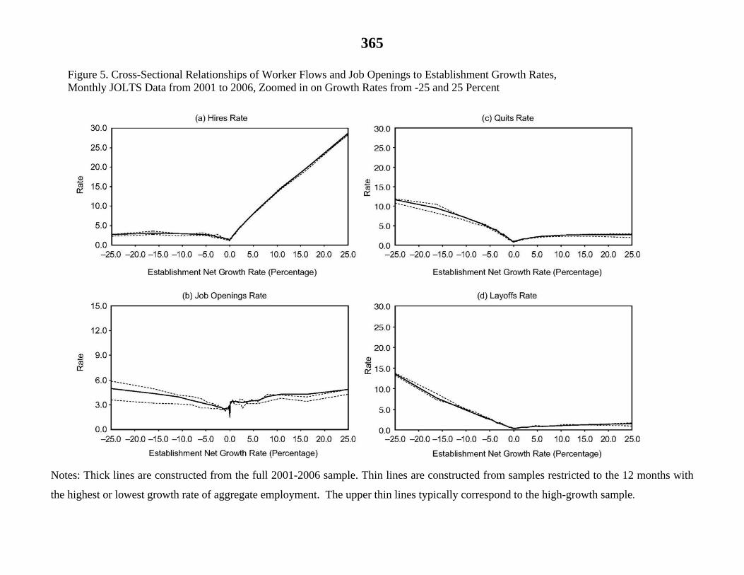
365
Figure 5. Cross-Sectional Relationships of Worker Flows and Job Openings to Establishment Growth Rates, Monthly JOLTS Data from 2001 to 2006, Zoomed in on Growth Rates from -25 and 25 Percent
Notes: Thick lines are constructed from the full 2001-2006 sample. Thin lines are constructed from samples restricted to the 12 months with
the highest or lowest growth rate of aggregate employment. The upper thin lines typically correspond to the high-growth sample.
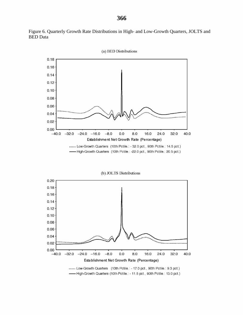
366
Figure 6. Quarterly Growth Rate Distributions in High- and Low-Growth Quarters, JOLTS and BED Data

367
Figure 6 Notes: Figures depict employment densities at establishments with quarterly growth
rates within a given interval in the BED (top panel) and a restricted panel of JOLTS data (bottom
panel, see text for details of restriction) for 2001Q1 – 2006Q4. The distributions are split into the
6 quarters of highest growth and 6 quarters of lowest growth, based on their seasonally
unadjusted aggregate growth rates in the BED. Vertical lines represent the growth rates at the
10th (shaded lines) and 90th (dashed lines) percentiles of the distribution, with the leftmost of
each pair associated with each low-growth distribution.
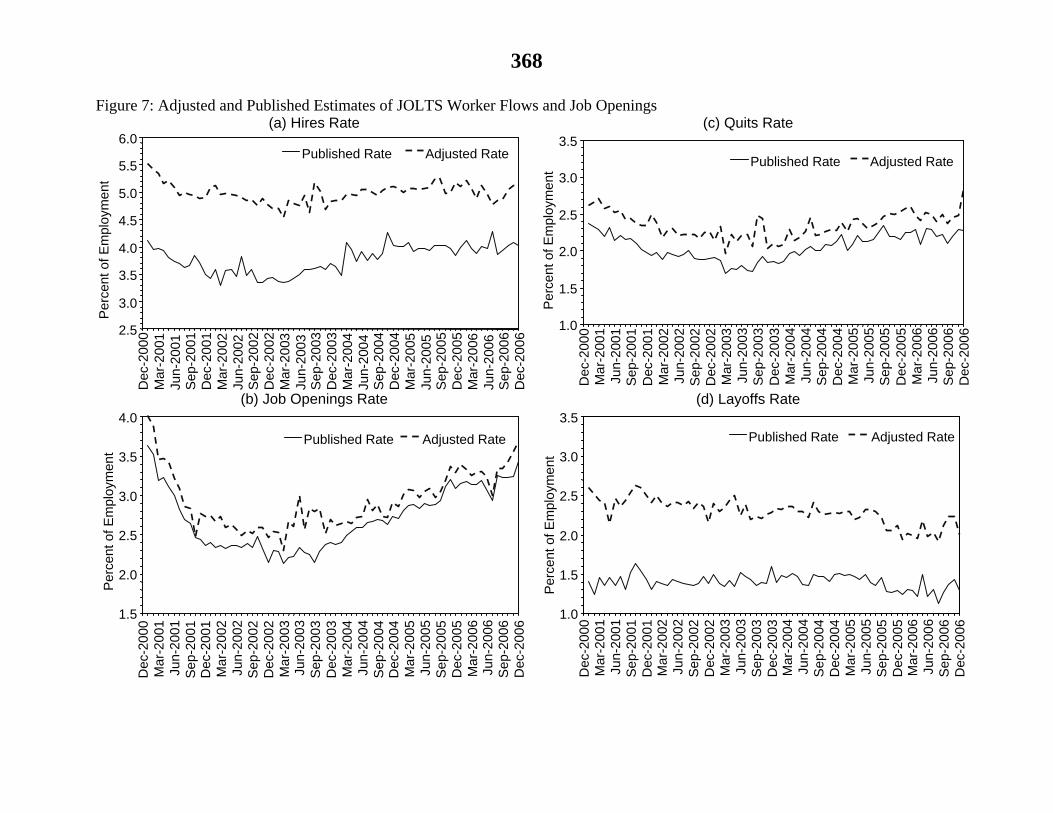
368
Figure 7: Adjusted and Published Estimates of JOLTS Worker Flows and Job Openings (a) Hires Rate
(b) Job Openings Rate
(c) Quits Rate
(d) Layoffs Rate
2.5
3.0
3.5
4.0
4.5
5.0
5.5
6.0 D
ec-2
000
Mar
-200
1 Ju
n-20
01
Sep
-200
1 D
ec-2
001
Mar
-200
2 Ju
n-20
02
Sep
-200
2 D
ec-2
002
Mar
-200
3 Ju
n-20
03
Sep
-200
3 D
ec-2
003
Mar
-200
4 Ju
n-20
04
Sep
-200
4 D
ec-2
004
Mar
-200
5 Ju
n-20
05
Sep
-200
5 D
ec-2
005
Mar
-200
6 Ju
n-20
06
Sep
-200
6 D
ec-2
006
Per
cent
of E
mpl
oym
ent
Published Rate Adjusted Rate
1.0
1.5
2.0
2.5
3.0
3.5
Dec
-200
0 M
ar-2
001
Jun-
2001
S
ep-2
001
Dec
-200
1 M
ar-2
002
Jun-
2002
S
ep-2
002
Dec
-200
2 M
ar-2
003
Jun-
2003
S
ep-2
003
Dec
-200
3 M
ar-2
004
Jun-
2004
S
ep-2
004
Dec
-200
4 M
ar-2
005
Jun-
2005
S
ep-2
005
Dec
-200
5 M
ar-2
006
Jun-
2006
S
ep-2
006
Dec
-200
6
Per
cent
of E
mpl
oym
ent
Published Rate Adjusted Rate
1.5
2.0
2.5
3.0
3.5
4.0
Dec
-200
0 M
ar-2
001
Jun-
2001
S
ep-2
001
Dec
-200
1 M
ar-2
002
Jun-
2002
S
ep-2
002
Dec
-200
2 M
ar-2
003
Jun-
2003
S
ep-2
003
Dec
-200
3 M
ar-2
004
Jun-
2004
S
ep-2
004
Dec
-200
4 M
ar-2
005
Jun-
2005
S
ep-2
005
Dec
-200
5 M
ar-2
006
Jun-
2006
S
ep-2
006
Dec
-200
6
Per
cent
of E
mpl
oym
ent
Published Rate Adjusted Rate
1.0
1.5
2.0
2.5
3.0
3.5
Dec
-200
0 M
ar-2
001
Jun-
2001
S
ep-2
001
Dec
-200
1 M
ar-2
002
Jun-
2002
S
ep-2
002
Dec
-200
2 M
ar-2
003
Jun-
2003
S
ep-2
003
Dec
-200
3 M
ar-2
004
Jun-
2004
S
ep-2
004
Dec
-200
4 M
ar-2
005
Jun-
2005
S
ep-2
005
Dec
-200
5 M
ar-2
006
Jun-
2006
S
ep-2
006
Dec
-200
6
Per
cent
of E
mpl
oym
ent
Published Rate Adjusted Rate

369
Figure 7 Notes: Each panel illustrates a worker flow or job openings rate, seasonally
adjusted, from the published JOLTS statistics (solid line) and our adjusted estimates
(dashed line). See text for details of the adjustment.
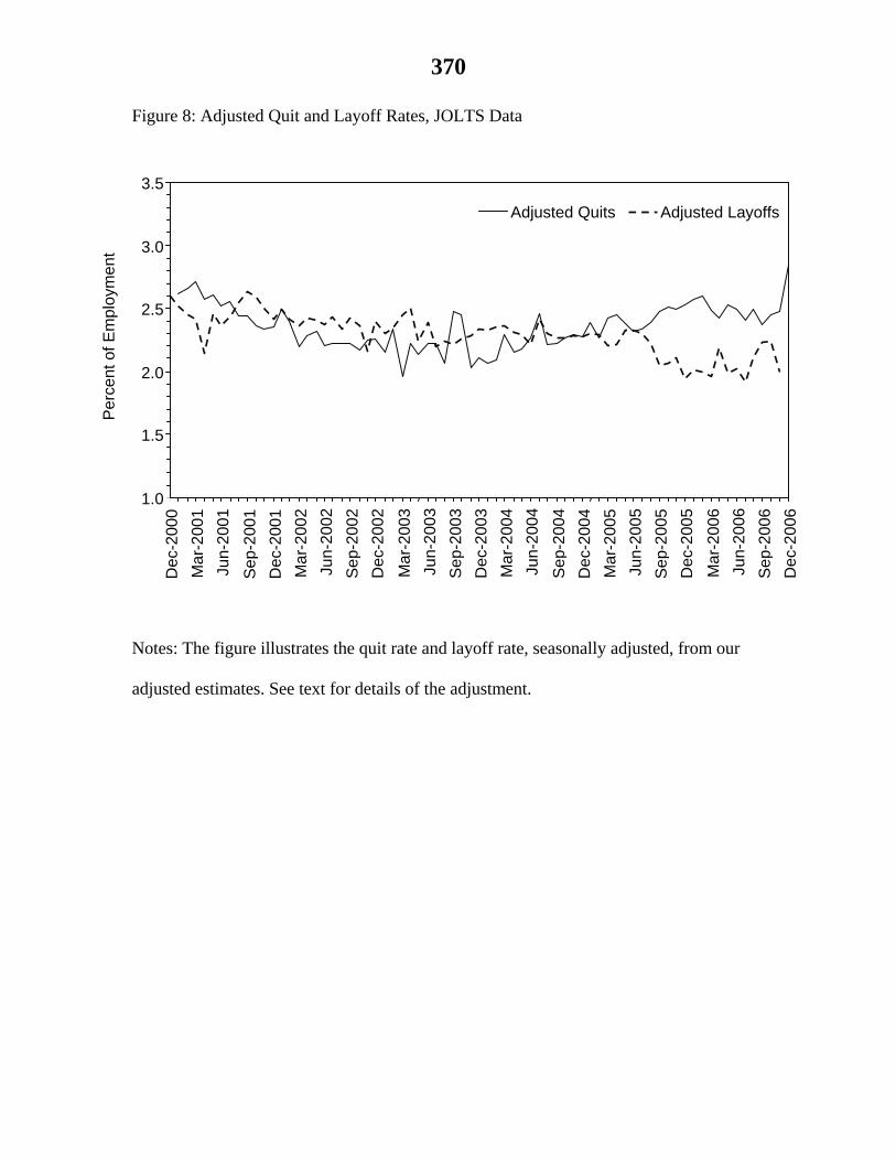
370
Figure 8: Adjusted Quit and Layoff Rates, JOLTS Data
Notes: The figure illustrates the quit rate and layoff rate, seasonally adjusted, from our
adjusted estimates. See text for details of the adjustment.
1.0
1.5
2.0
2.5
3.0
3.5 D
ec-2
000
Ma r
-200
1
Jun-
2001
Sep
-200
1
Dec
-200
1
Mar
-200
2
Jun-
2002
Sep
-200
2
Dec
-200
2
Ma r
-200
3
Jun-
2003
Se p
-200
3
Dec
-200
3
Mar
-200
4
Jun-
2004
Se p
-200
4
Dec
-200
4
Mar
-200
5
Jun-
2005
Sep
-200
5
Dec
-200
5
Ma r
-200
6
Jun-
2006
Se p
-200
6
Dec
-200
6
Per
cent
of E
mpl
oym
ent
Adjusted Quits Adjusted Layoffs