Embed Size (px)
Citation preview
Advanced Implementations of Tables: Balanced Search Trees and Hashing
Binary searching & introduction to trees 2CMPS 12B, UC Santa Cruz
Balanced Search Trees
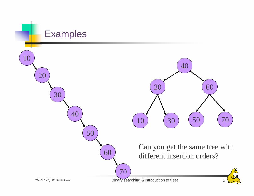
Binary search tree operations such as insert, delete, retrieve, etc. depend on the length of the path to the desired nodeThe path length can vary from log2(n+1) to O(n) depending on how balanced or unbalanced the tree isThe shape of the tree is determined by the values of the items and the order in which they were inserted
Binary searching & introduction to trees 3CMPS 12B, UC Santa Cruz
Examples
40
20 60
503010 70
10
40
20
70
50
60
30
Can you get the same tree with different insertion orders?
Binary searching & introduction to trees 4CMPS 12B, UC Santa Cruz
2-3 Trees
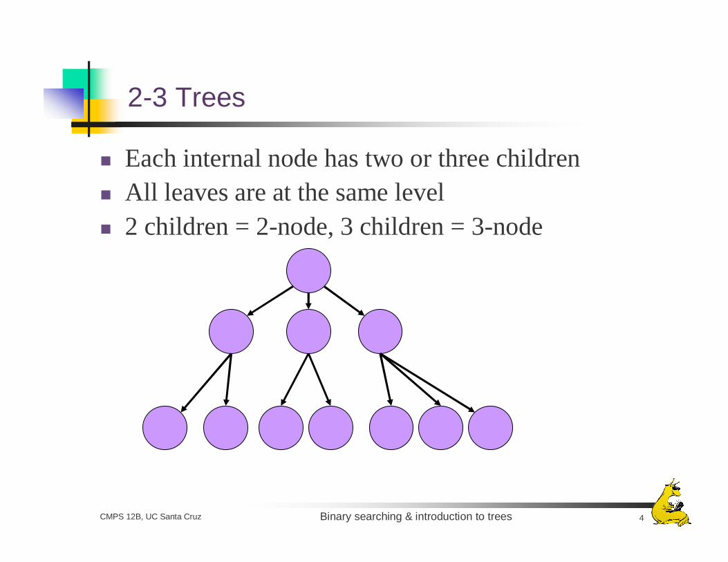
Each internal node has two or three childrenAll leaves are at the same level2 children = 2-node, 3 children = 3-node
Binary searching & introduction to trees 5CMPS 12B, UC Santa Cruz
2-3 Trees (continued)
2-3 trees are not binary trees (duh)A 2-3 tree of height h always has at least 2h-1 nodes
i.e. greater than or equal to a binary tree of height h
A 2-3 tree with n nodes has height less than or equal to log2(n+1)
i.e less than or equal to the height of a full binary tree with n nodes
Binary searching & introduction to trees 6CMPS 12B, UC Santa Cruz
Definition of 2-3 Trees
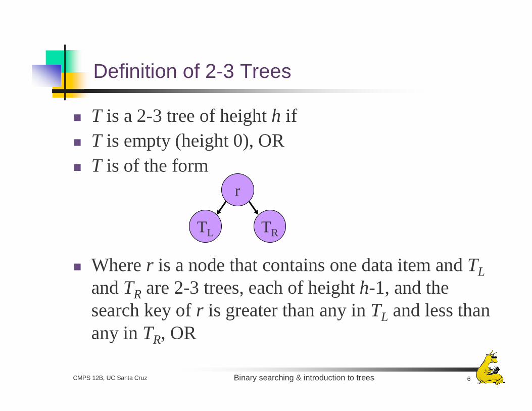
T is a 2-3 tree of height h ifT is empty (height 0), ORT is of the form
Where r is a node that contains one data item and TL
and TR are 2-3 trees, each of height h-1, and the search key of r is greater than any in TL and less than any in TR, OR
r
TL TR
Binary searching & introduction to trees 7CMPS 12B, UC Santa Cruz
Definition of 2-3 Trees (continued)
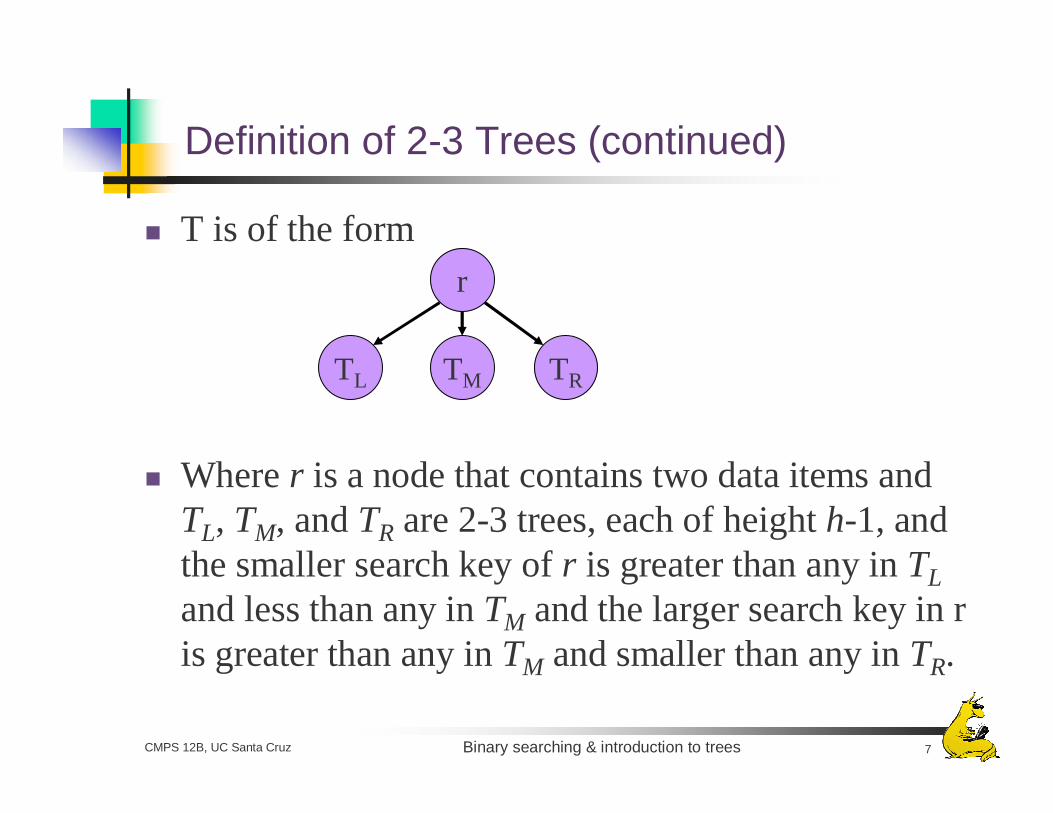
T is of the form
Where r is a node that contains two data items and TL, TM, and TR are 2-3 trees, each of height h-1, and the smaller search key of r is greater than any in TL
and less than any in TM and the larger search key in r is greater than any in TM and smaller than any in TR.
r
TL TRTM
Binary searching & introduction to trees 8CMPS 12B, UC Santa Cruz
Placing Data in a 2-3 tree
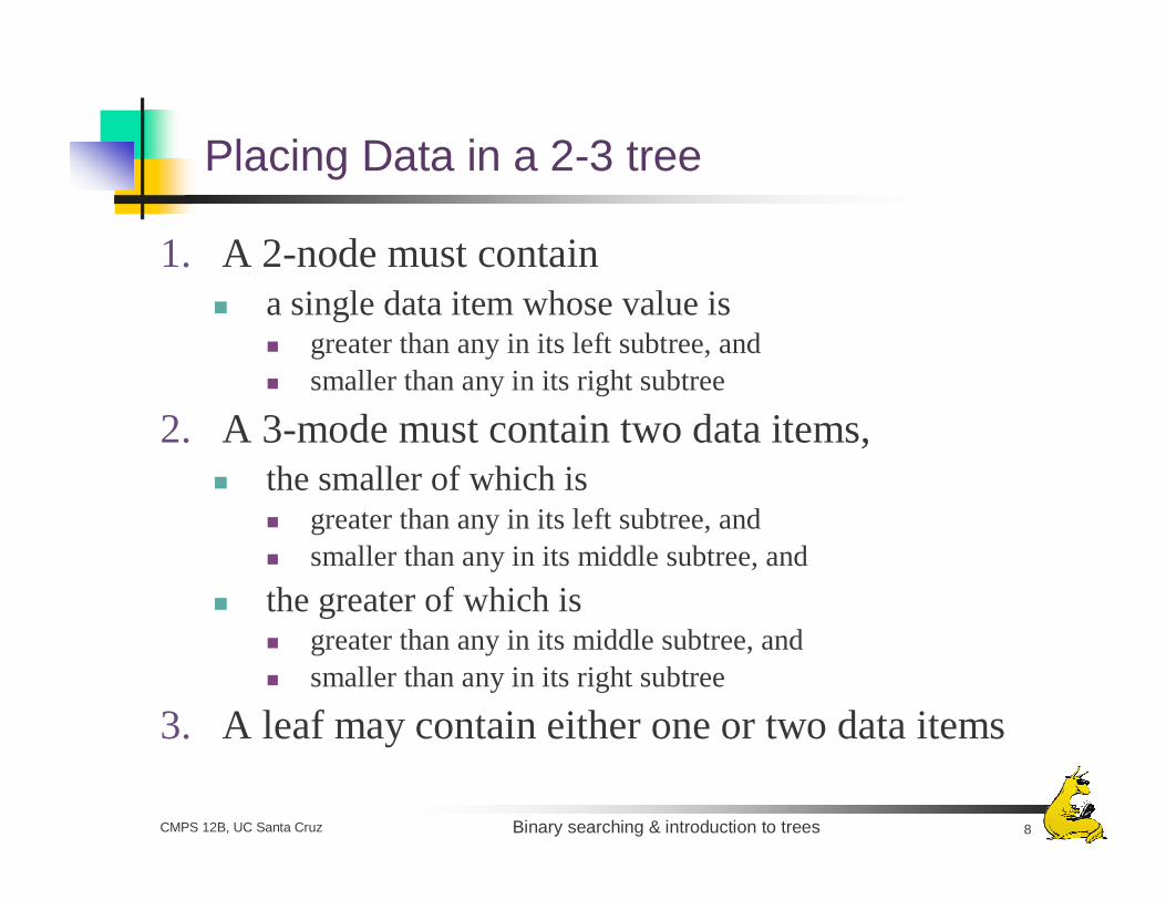
1. A 2-node must contain a single data item whose value is
greater than any in its left subtree, and smaller than any in its right subtree
2. A 3-mode must contain two data items, the smaller of which is
greater than any in its left subtree, and smaller than any in its middle subtree, and
the greater of which is greater than any in its middle subtree, and smaller than any in its right subtree
3. A leaf may contain either one or two data items
Binary searching & introduction to trees 9CMPS 12B, UC Santa Cruz
2-3 Node Code
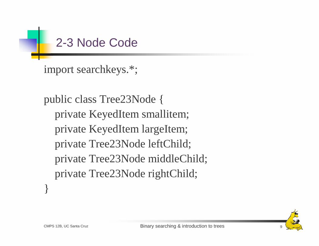
import searchkeys.*;
public class Tree23Node {private KeyedItem smallitem;private KeyedItem largeItem;private Tree23Node leftChild;private Tree23Node middleChild;private Tree23Node rightChild;
}
Binary searching & introduction to trees 10CMPS 12B, UC Santa Cruz
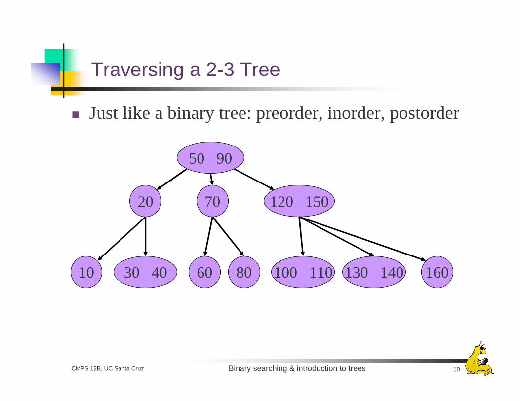
Traversing a 2-3 Tree
Just like a binary tree: preorder, inorder, postorder
50 90
20 120 150
100 11030 4010 130 140
70
16060 80
Binary searching & introduction to trees 11CMPS 12B, UC Santa Cruz
Searching a 2-3 tree
Same efficiency as a balanced binary search tree: O(logn)BUT, easy to keep balanced, unlike binary search treesThis means that as you insert elements, the balance is easily maintained, and worst case performance remains O(logn)
Binary searching & introduction to trees 12CMPS 12B, UC Santa Cruz
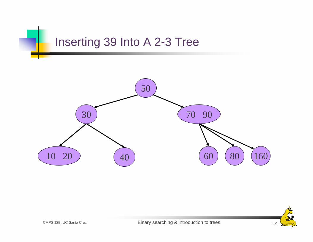
Inserting 39 Into A 2-3 Tree
50
30 70 90
6010 20 80 16040
Binary searching & introduction to trees 13CMPS 12B, UC Santa Cruz
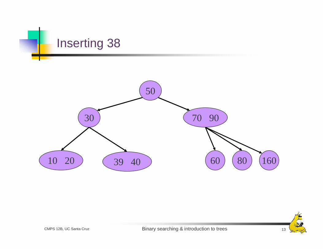
Inserting 38
50
30 70 90
6010 20 80 16039 40
Binary searching & introduction to trees 14CMPS 12B, UC Santa Cruz
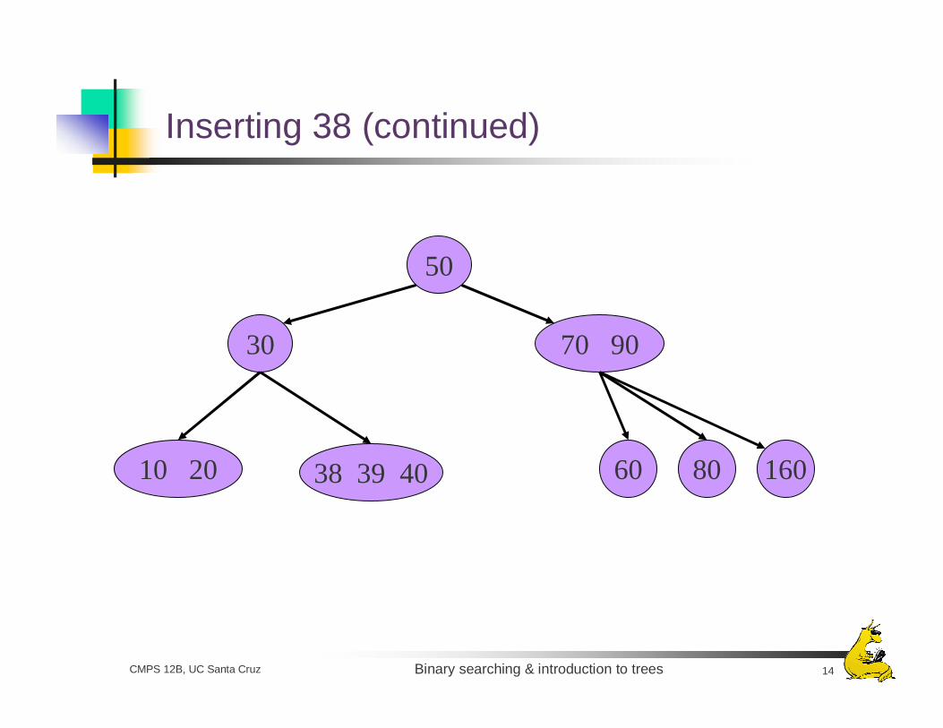
Inserting 38 (continued)
50
30 70 90
6010 20 80 16038 39 40
Binary searching & introduction to trees 15CMPS 12B, UC Santa Cruz
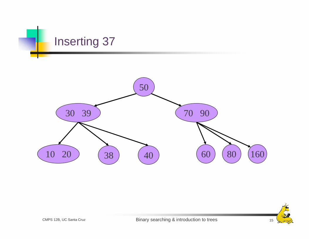
Inserting 37
50
30 39 70 90
6010 20 80 16038 40
Binary searching & introduction to trees 16CMPS 12B, UC Santa Cruz
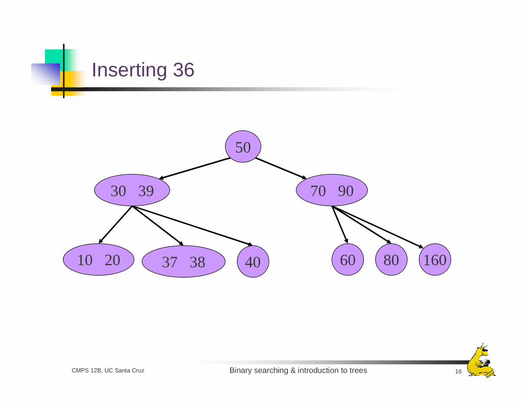
Inserting 36
50
30 39 70 90
6010 20 80 16037 38 40
Binary searching & introduction to trees 17CMPS 12B, UC Santa Cruz
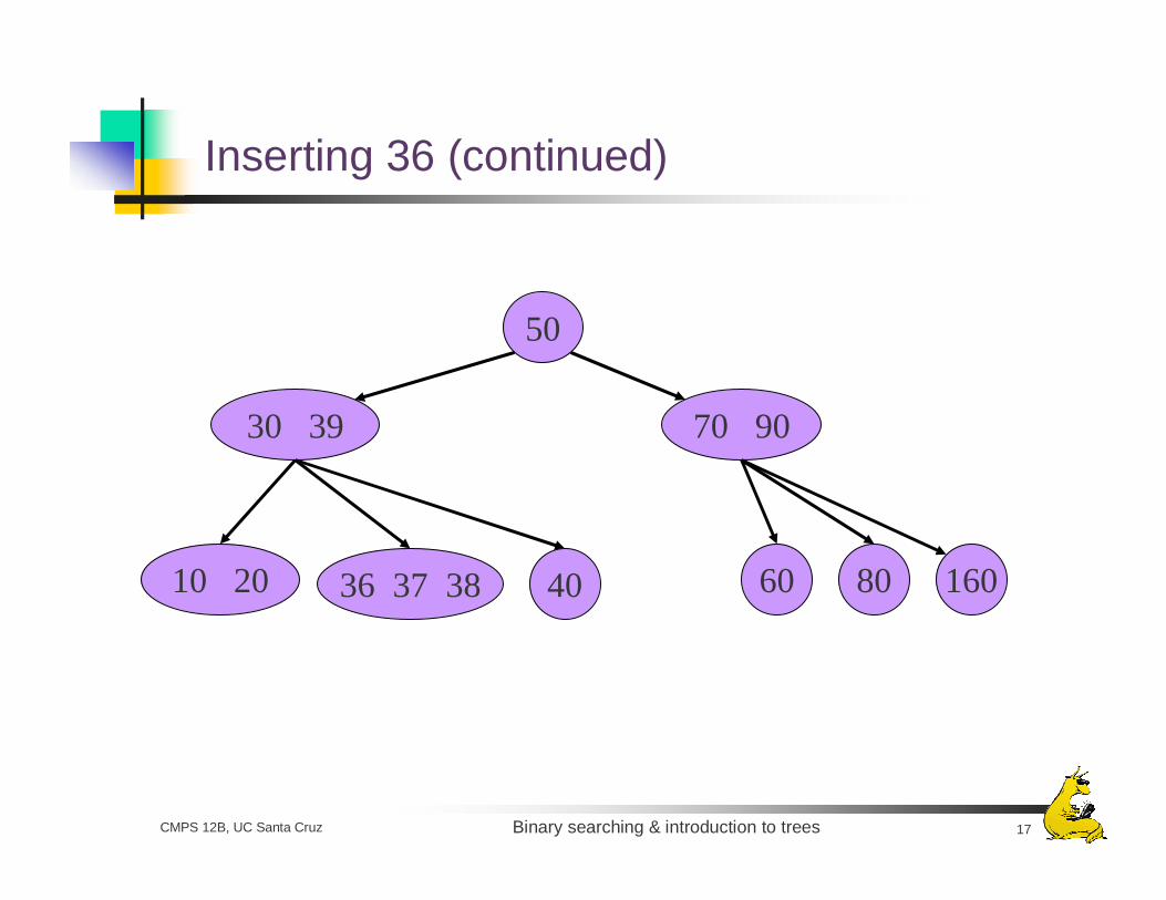
Inserting 36 (continued)
50
30 39 70 90
6010 20 80 16036 37 38 40
Binary searching & introduction to trees 18CMPS 12B, UC Santa Cruz
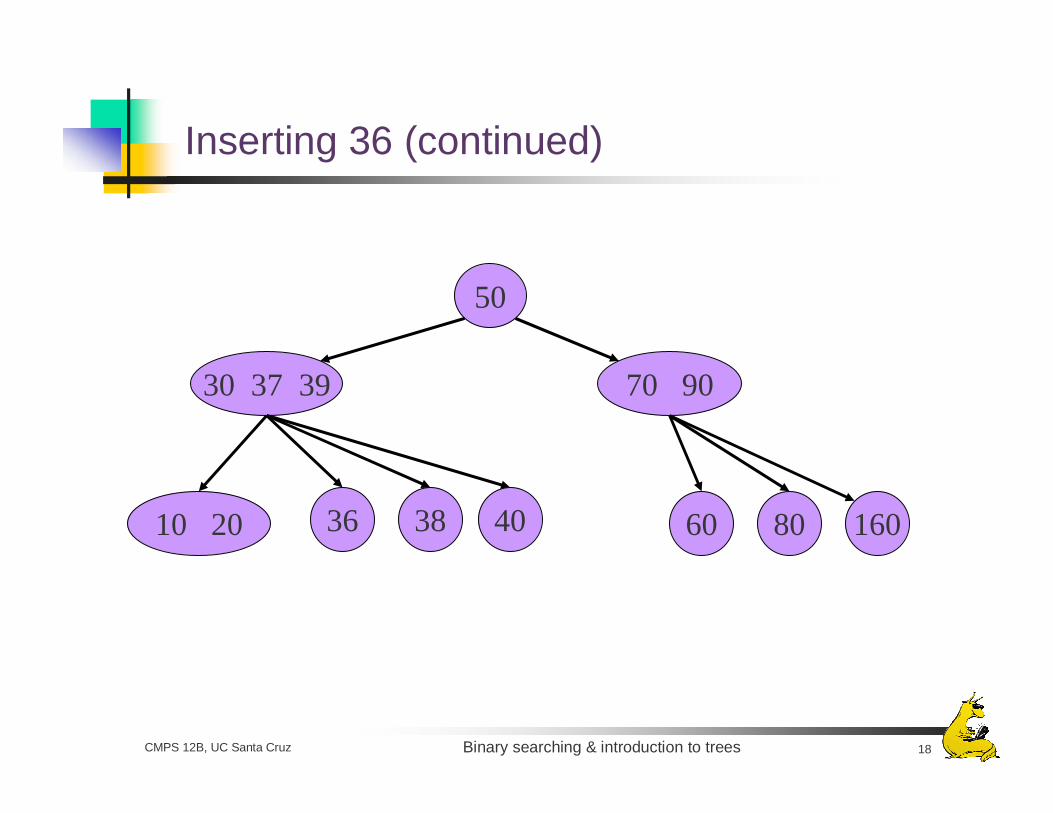
Inserting 36 (continued)
50
30 37 39 70 90
6010 20 80 16036 4038
Binary searching & introduction to trees 19CMPS 12B, UC Santa Cruz
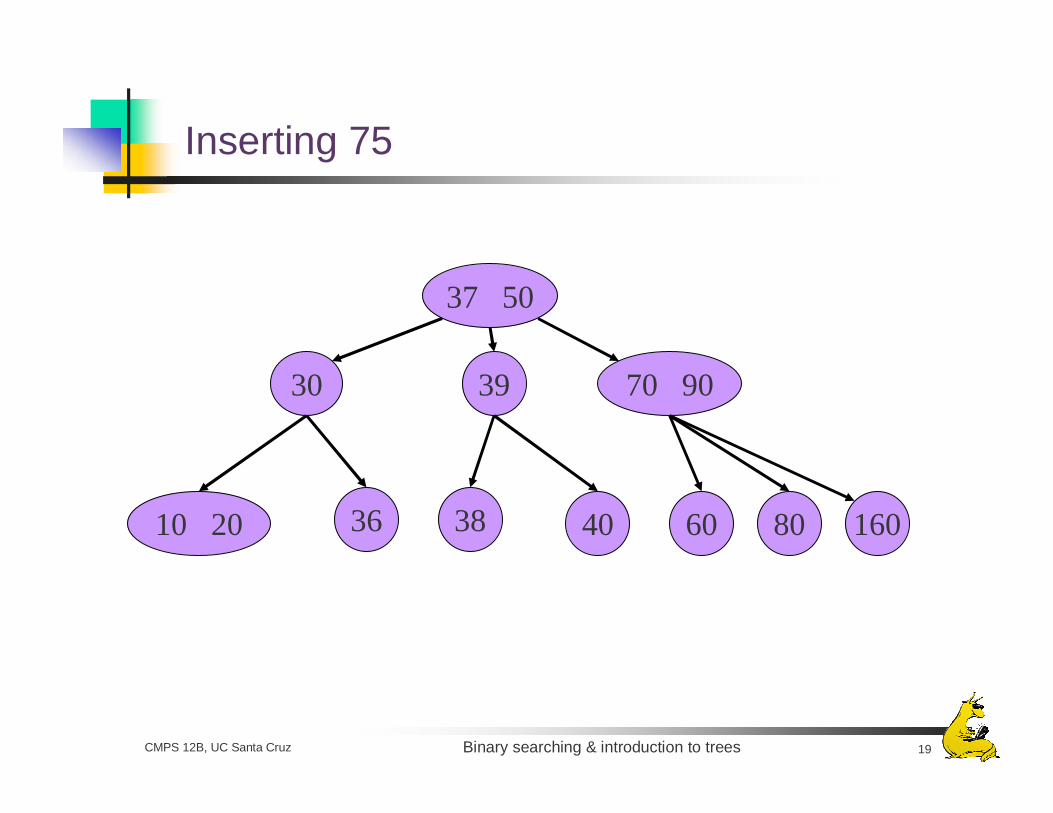
Inserting 75
37 50
30 70 90
6010 20 80
39
16036 4038
Binary searching & introduction to trees 20CMPS 12B, UC Santa Cruz
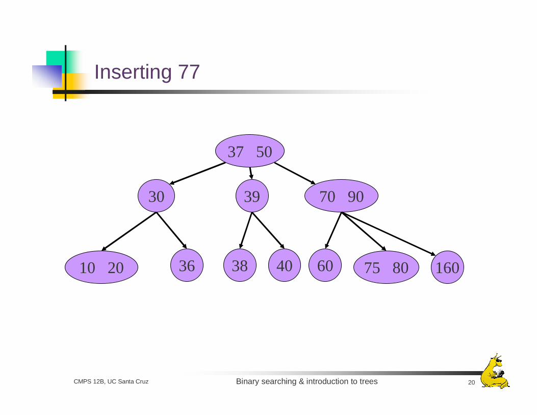
Inserting 77
37 50
30 70 90
6010 20 75 80
39
16036 4038

Binary searching & introduction to trees 21CMPS 12B, UC Santa Cruz
Inserting 77 (continued)
37 50
30 70 90
6010 20 75 77 80
39
16036 4038

Binary searching & introduction to trees 22CMPS 12B, UC Santa Cruz
Inserting 77 (continued)
37 50
30 70 77 90
6010 20 75
39
16036 4038 80
Binary searching & introduction to trees 23CMPS 12B, UC Santa Cruz
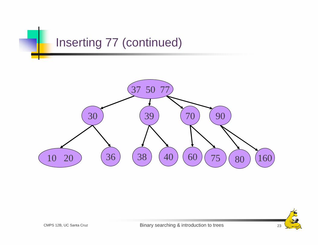
Inserting 77 (continued)
37 50 77
30 70
6010 20 75
39
16036 4038 80
90
Binary searching & introduction to trees 24CMPS 12B, UC Santa Cruz
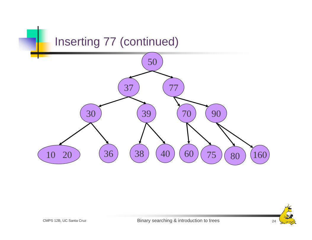
Inserting 77 (continued)
37
30 70
6010 20 75
39
16036 4038 80
90
77
50
Binary searching & introduction to trees 25CMPS 12B, UC Santa Cruz
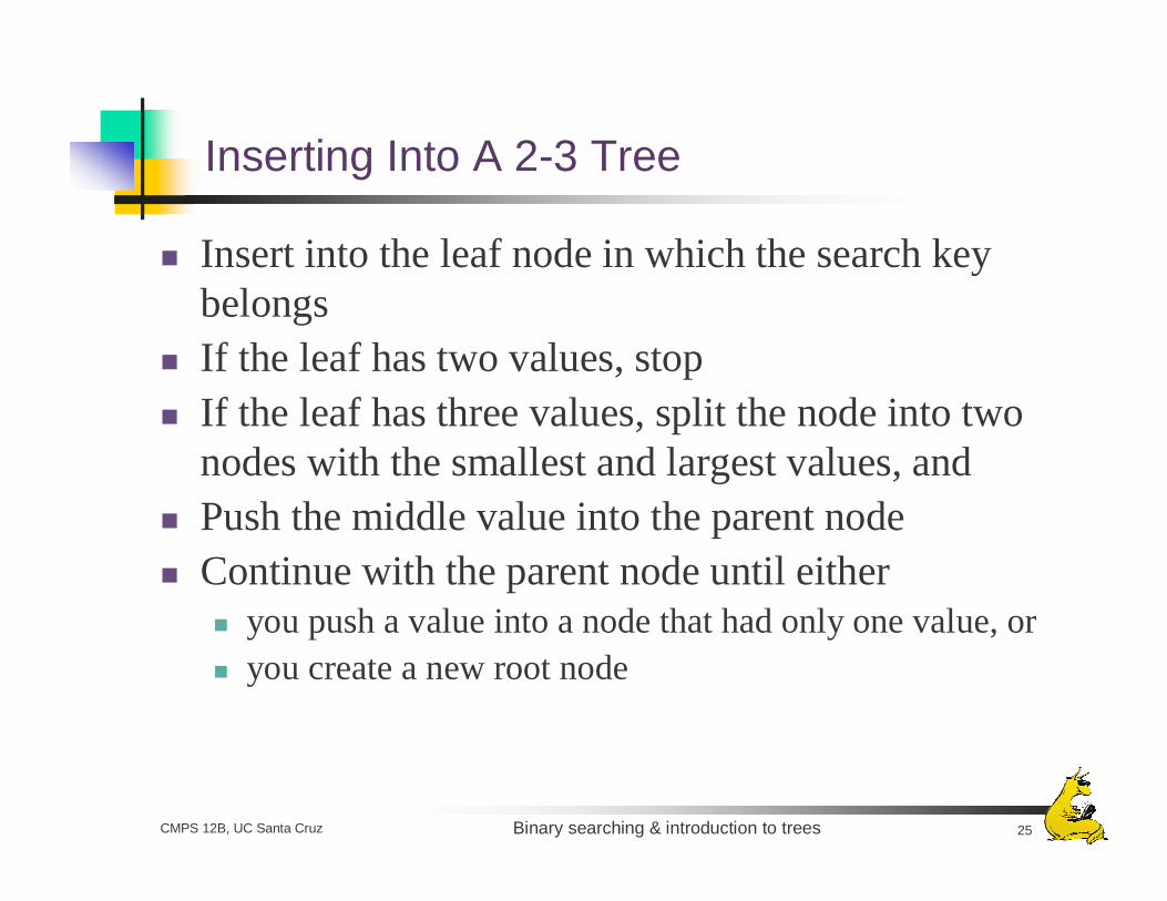
Inserting Into A 2-3 Tree
Insert into the leaf node in which the search key belongsIf the leaf has two values, stopIf the leaf has three values, split the node into two nodes with the smallest and largest values, andPush the middle value into the parent nodeContinue with the parent node until either
you push a value into a node that had only one value, oryou create a new root node
Binary searching & introduction to trees 26CMPS 12B, UC Santa Cruz
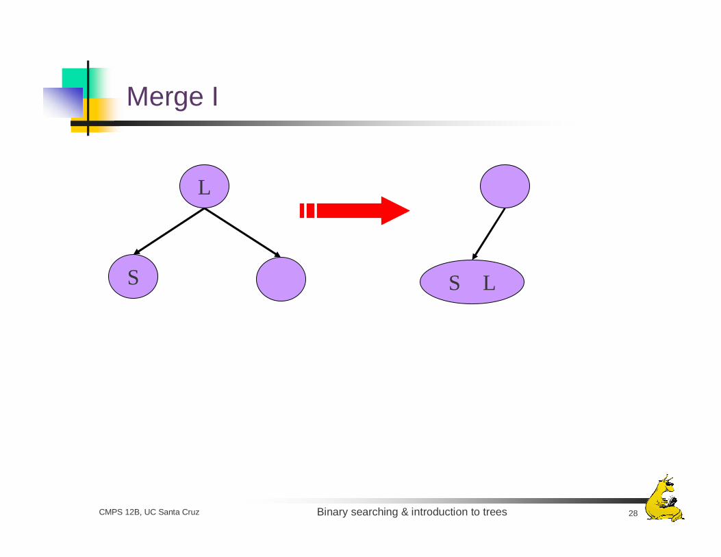
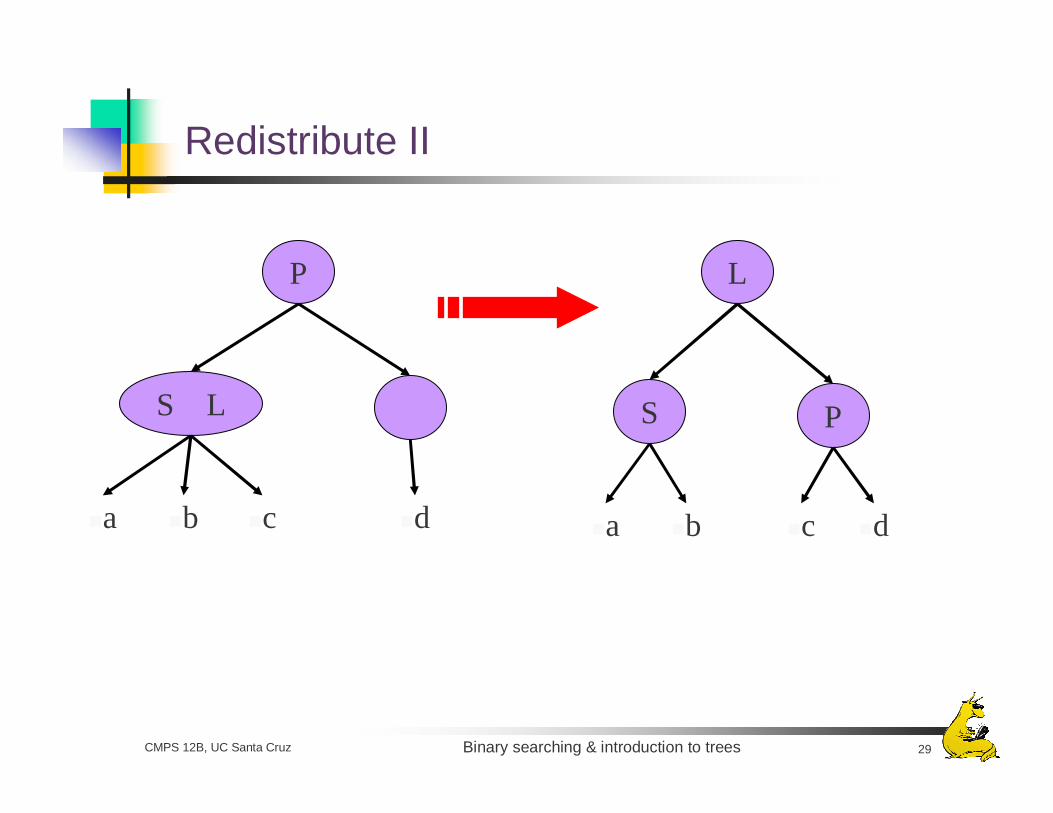
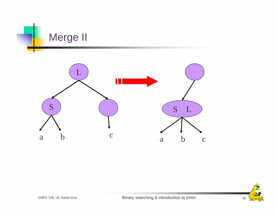
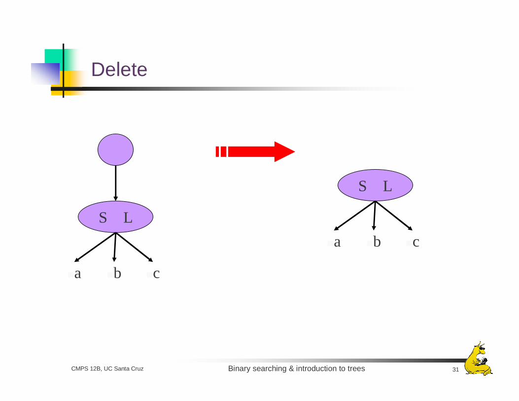
Deleting From A 2-3 Tree
The inverse of insertingDelete the value (in a leaf), thenMerge empty nodesIf necessary, delete empty root
Binary searching & introduction to trees 27CMPS 12B, UC Santa Cruz
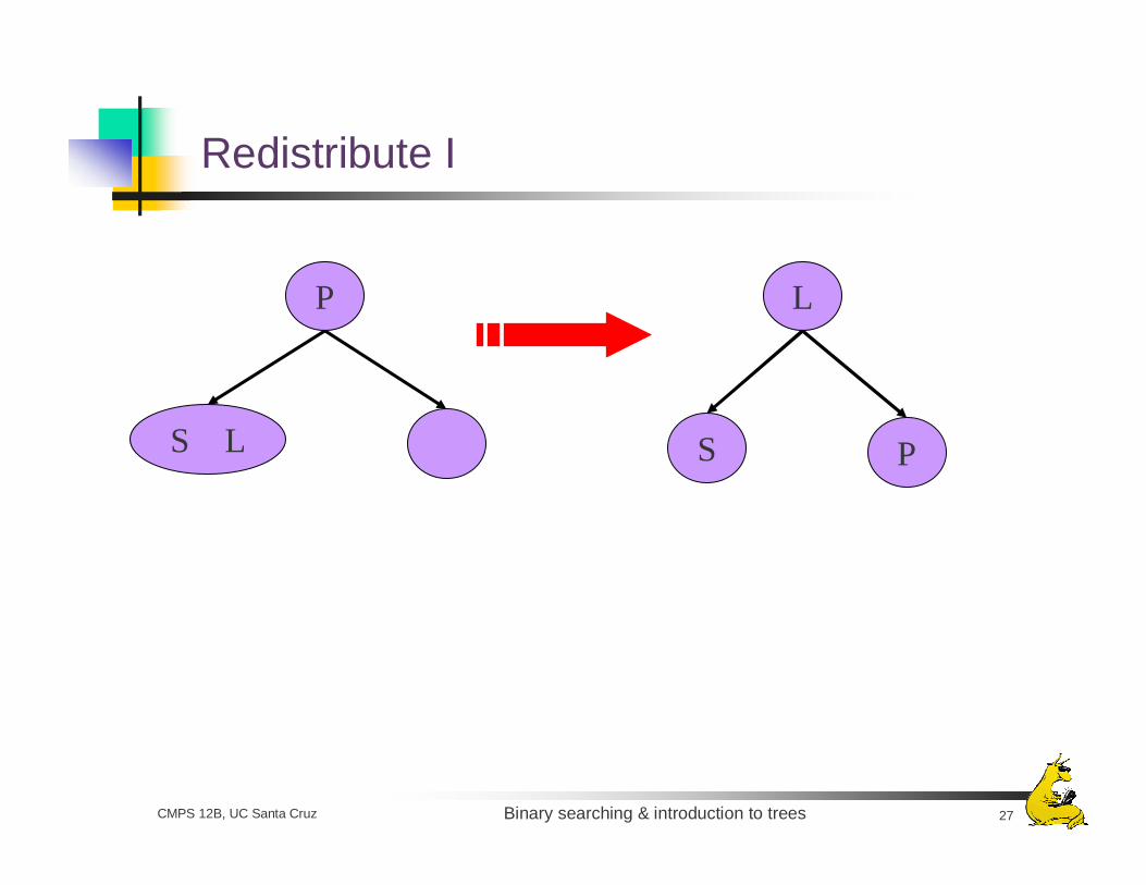
Redistribute I
P
S L
L
S P
Binary searching & introduction to trees 28CMPS 12B, UC Santa Cruz
Merge I
L
S S L
Binary searching & introduction to trees 29CMPS 12B, UC Santa Cruz
Redistribute II
P
S L
L
S P
a b c d a b c d
Binary searching & introduction to trees 30CMPS 12B, UC Santa Cruz
Merge II
L
S S L
a b c a b c
Binary searching & introduction to trees 31CMPS 12B, UC Santa Cruz
Delete
S L
a b c
S L
a b c
Binary searching & introduction to trees 32CMPS 12B, UC Santa Cruz
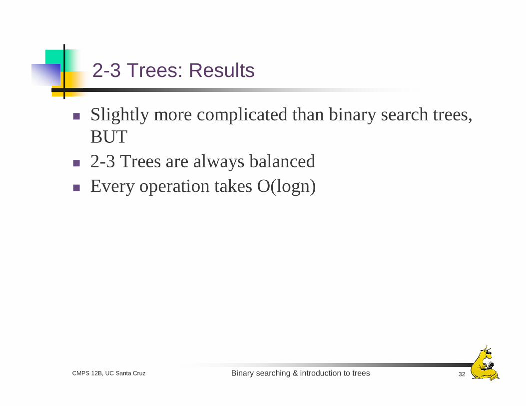
2-3 Trees: Results
Slightly more complicated than binary search trees, BUT2-3 Trees are always balancedEvery operation takes O(logn)
Binary searching & introduction to trees 33CMPS 12B, UC Santa Cruz
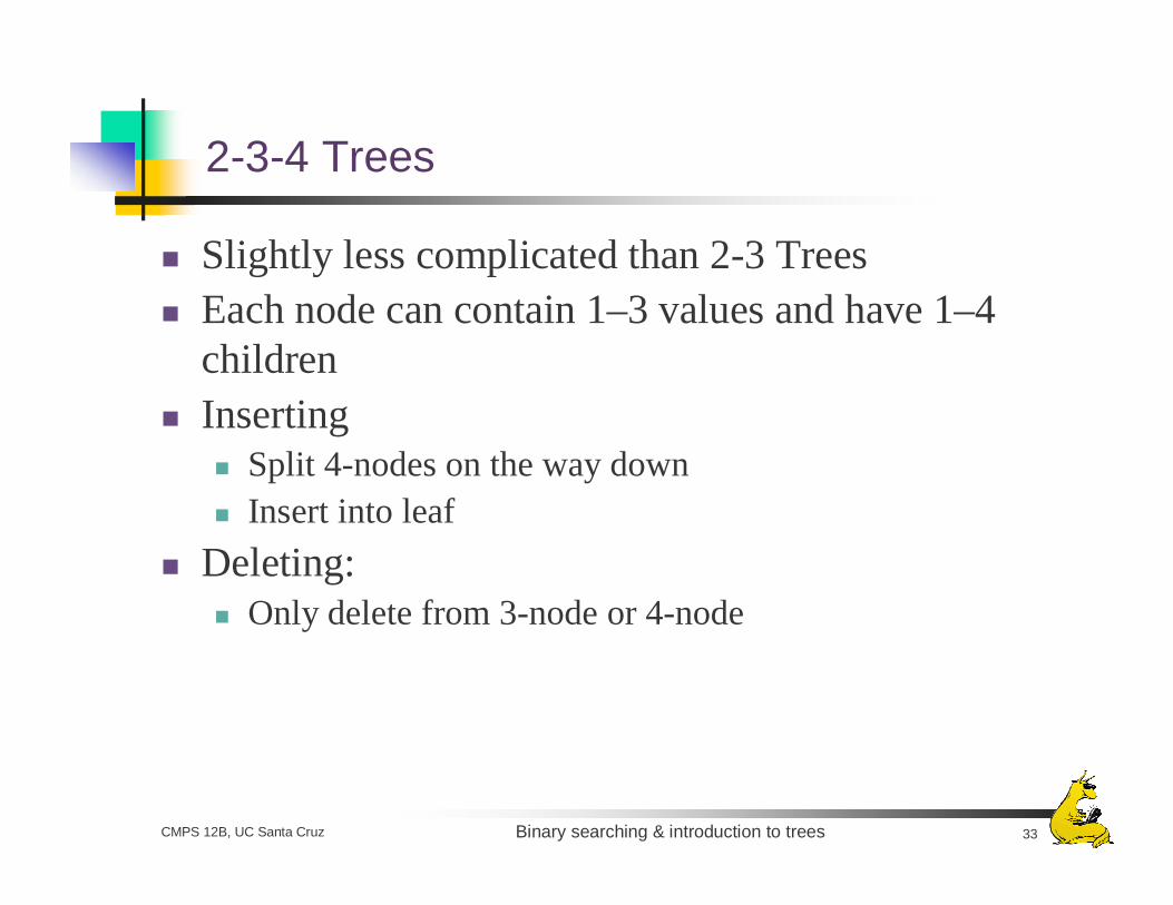
2-3-4 Trees
Slightly less complicated than 2-3 TreesEach node can contain 1–3 values and have 1–4 childrenInserting
Split 4-nodes on the way downInsert into leaf
Deleting: Only delete from 3-node or 4-node
Binary searching & introduction to trees 34CMPS 12B, UC Santa Cruz
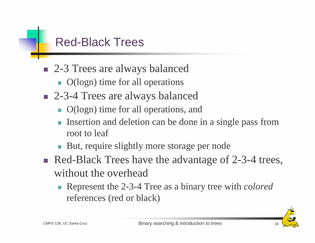
Red-Black Trees
2-3 Trees are always balancedO(logn) time for all operations
2-3-4 Trees are always balancedO(logn) time for all operations, andInsertion and deletion can be done in a single pass from root to leafBut, require slightly more storage per node
Red-Black Trees have the advantage of 2-3-4 trees, without the overhead
Represent the 2-3-4 Tree as a binary tree with coloredreferences (red or black)
Binary searching & introduction to trees 35CMPS 12B, UC Santa Cruz
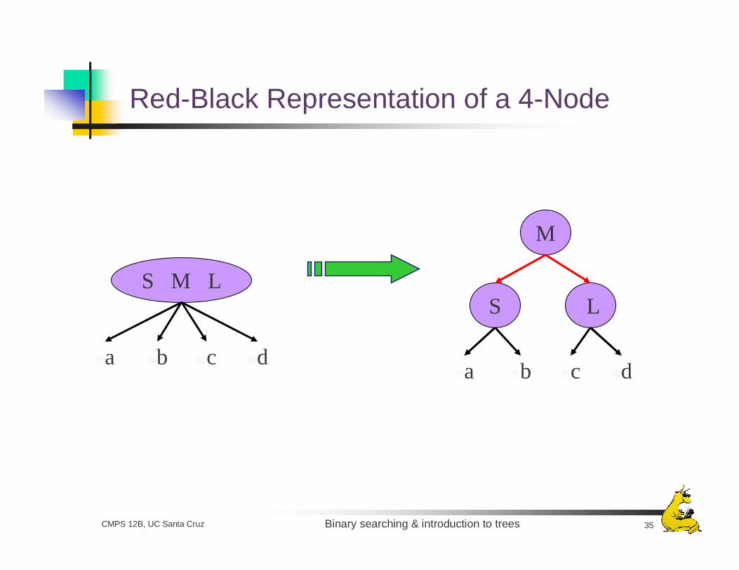
Red-Black Representation of a 4-Node
S M L
a b c d
M
S L
a b c d
Binary searching & introduction to trees 36CMPS 12B, UC Santa Cruz
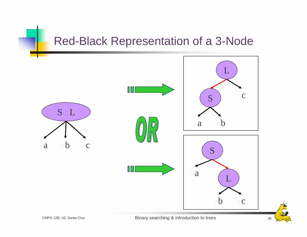
Red-Black Representation of a 3-Node
S L
a b c
L
S
a b
c
S
L
b c
a
Binary searching & introduction to trees 37CMPS 12B, UC Santa Cruz
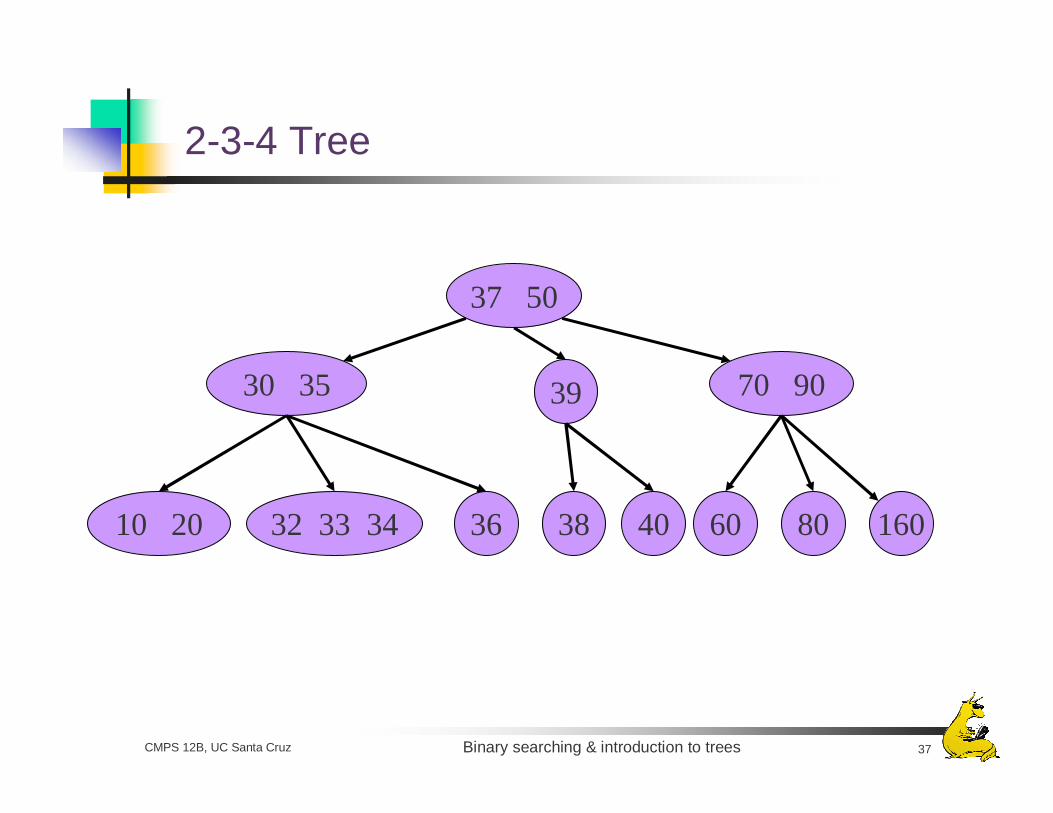
2-3-4 Tree
37 50
30 35 70 90
6010 20 80
39
16032 33 34 403836
Binary searching & introduction to trees 38CMPS 12B, UC Santa Cruz
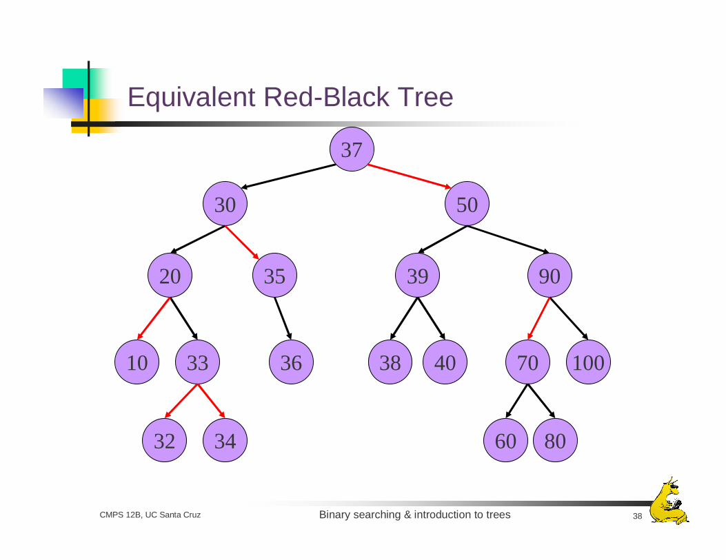
Equivalent Red-Black Tree
5030
90
70
20
100
39
80
33 403836
37
35
10
32 34 60
Binary searching & introduction to trees 39CMPS 12B, UC Santa Cruz
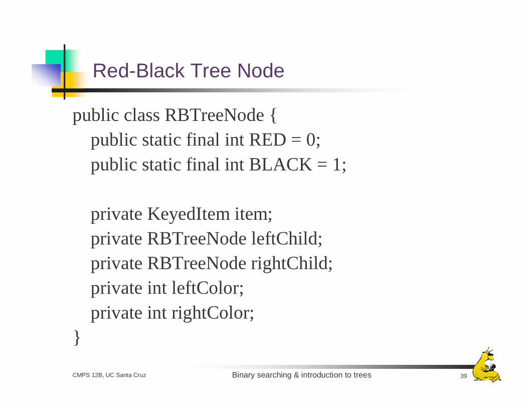
Red-Black Tree Node
public class RBTreeNode {public static final int RED = 0;public static final int BLACK = 1;
private KeyedItem item;private RBTreeNode leftChild;private RBTreeNode rightChild;private int leftColor;private int rightColor;
}
Binary searching & introduction to trees 40CMPS 12B, UC Santa Cruz
Searching and Traversing Red-Black Trees
Red-Black trees are binary search treesJust search them the same way you would any other binary search tree
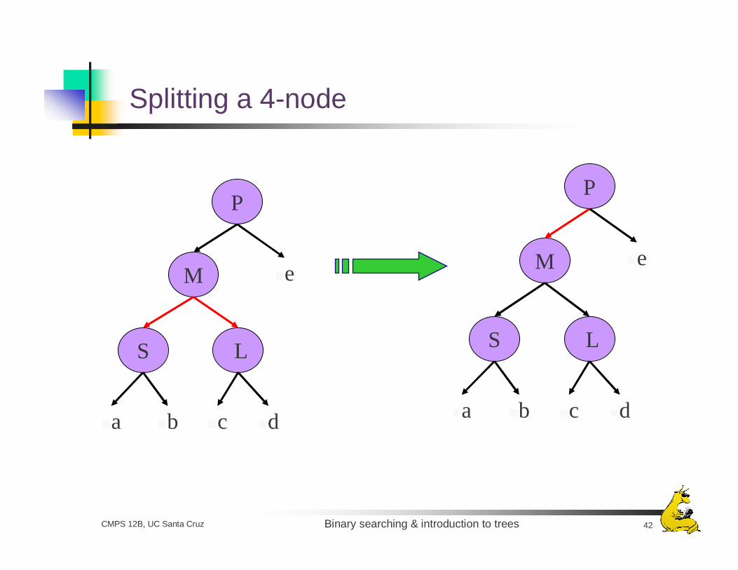
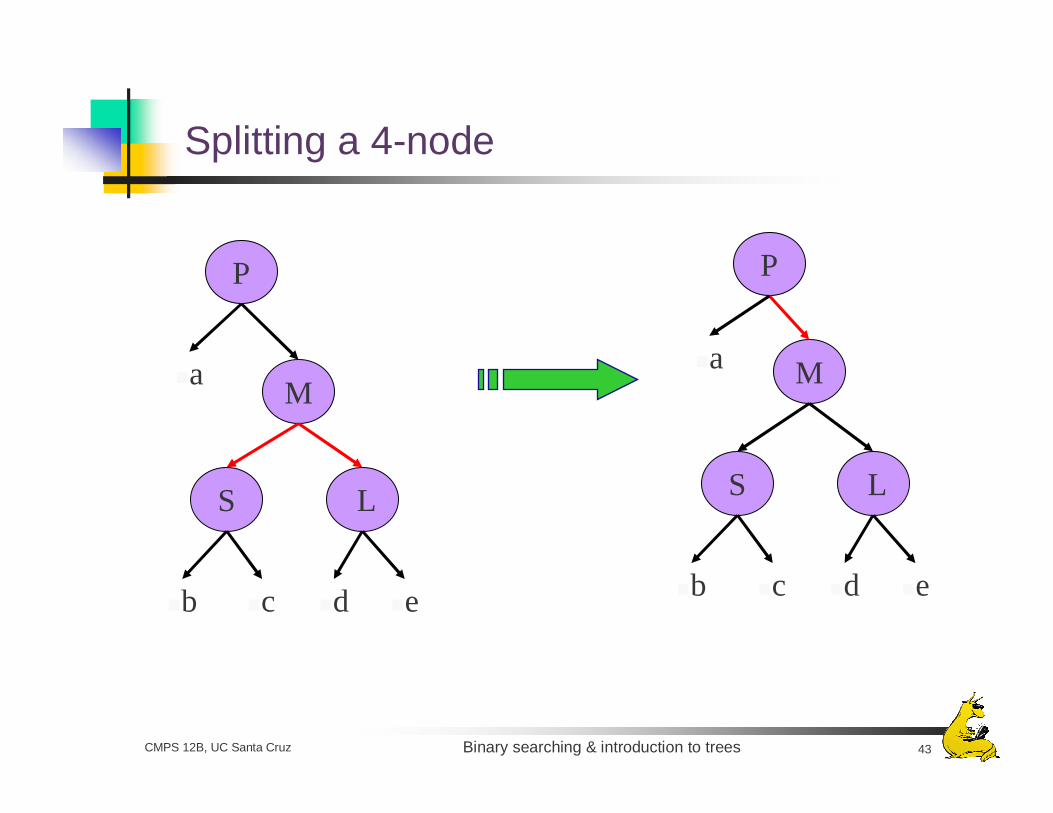
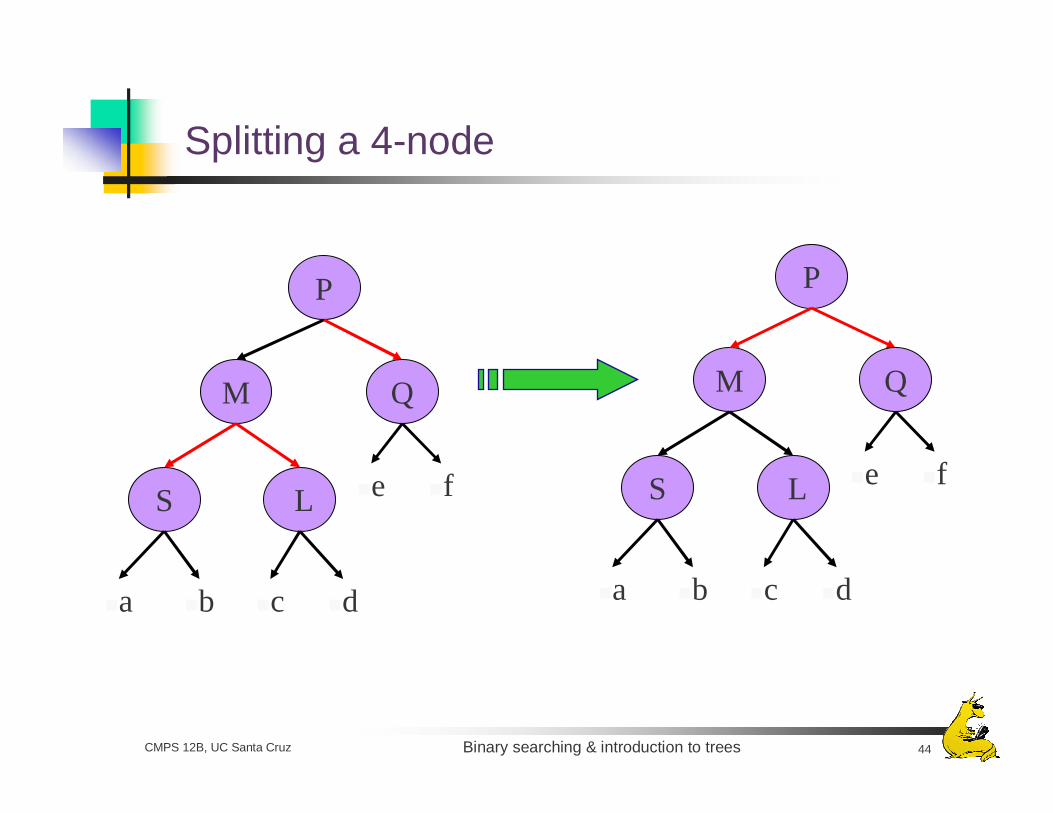
InsertingSplit 4-nodes on the way down by changing paired red child references to blackInsert into a leaf

Binary searching & introduction to trees 41CMPS 12B, UC Santa Cruz
Splitting a 4-node root
M
S L
a b c d
M
S L
a b c d
Binary searching & introduction to trees 42CMPS 12B, UC Santa Cruz
Splitting a 4-node
M
S L
a b c d
M
S L
a b c d
P
e
P
e
Binary searching & introduction to trees 43CMPS 12B, UC Santa Cruz
Splitting a 4-node
M
S L
b c d e
M
S L
b c d e
P
a
P
a
Binary searching & introduction to trees 44CMPS 12B, UC Santa Cruz
Splitting a 4-node
M
S L
a b c d
P
e
Q
f
M
S L
a b c d
P
e
Q
f
Binary searching & introduction to trees 45CMPS 12B, UC Santa Cruz
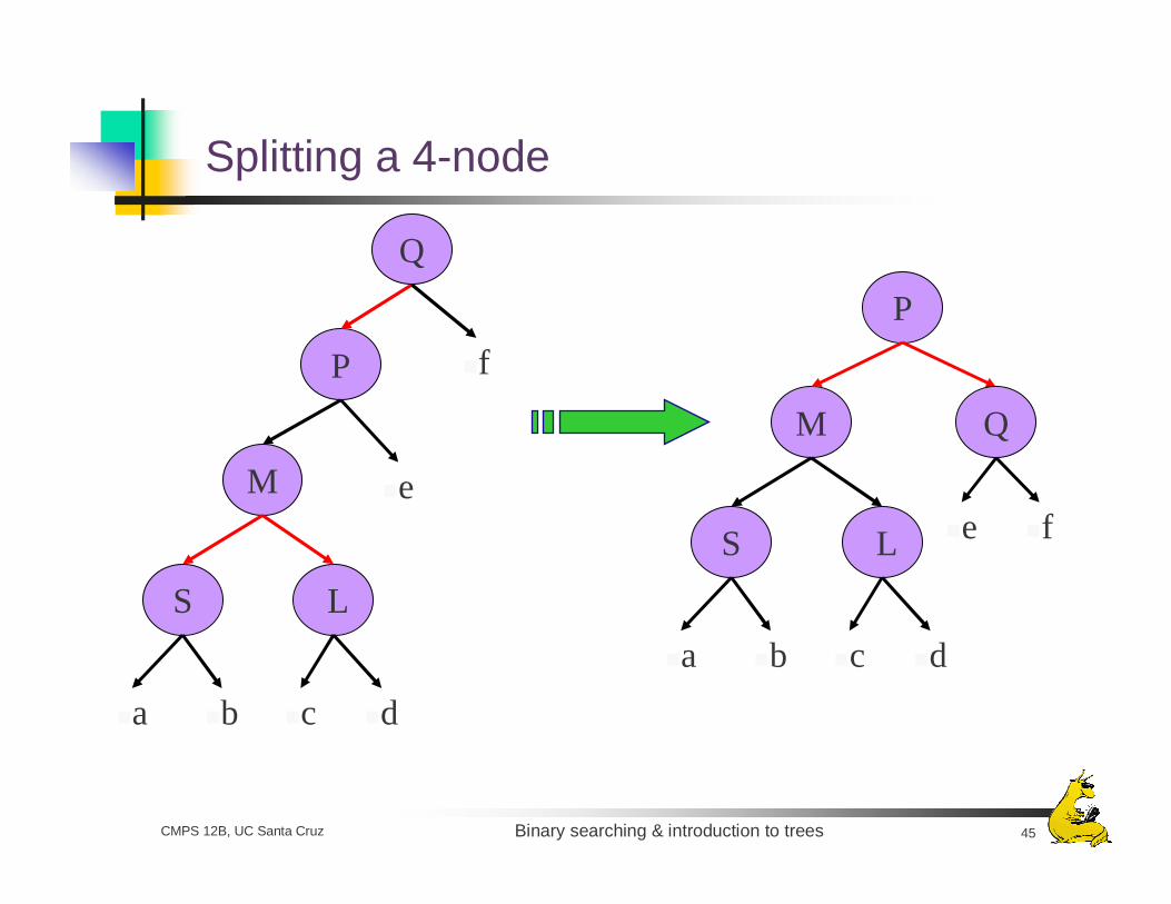
Splitting a 4-node
M
S L
a b c d
P
e
Q
f
M
S L
a b c d
P
e
Q
f
Binary searching & introduction to trees 46CMPS 12B, UC Santa Cruz
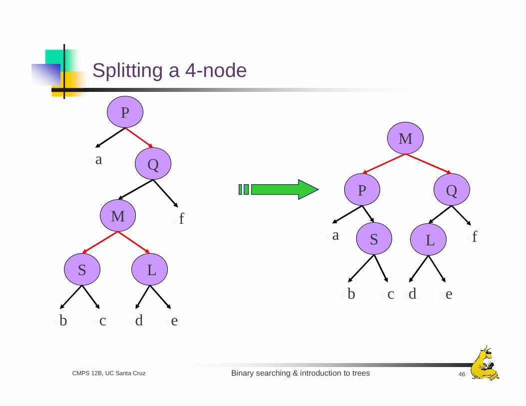
Splitting a 4-node
M
S L
b c d e
Q
f
P
a
P
L
d e
M
a
Q
fS
b c
Binary searching & introduction to trees 47CMPS 12B, UC Santa Cruz
AVL Trees
Insert in the appropriate spotRotate as necessary to restore balance
Rotate your way back up the tree
Every operation is O(logn)
Binary searching & introduction to trees 48CMPS 12B, UC Santa Cruz
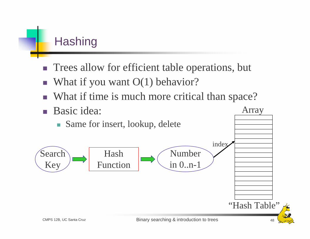
Hashing
Trees allow for efficient table operations, butWhat if you want O(1) behavior?What if time is much more critical than space?Basic idea:
Same for insert, lookup, delete
HashFunction
SearchKey
Numberin 0..n-1
Array
index
“Hash Table”
Binary searching & introduction to trees 49CMPS 12B, UC Santa Cruz
Issues
How to create a hash functionEasy or difficult, depending upon the desired properties
How large the array should beFactors: how many items will be stored, how much memory you have, how fast you want the operations to be
Static or dynamicHash collisions: what if two input values produce the same hash value?
Binary searching & introduction to trees 50CMPS 12B, UC Santa Cruz
Hash Functions
GoalsFast, easy to computeDistributes hash values evenly in the target range
Possible functions for an n-entry hash tableh(k) = random number in 0..n-1h(k) = the sum of the digits in kh(k) = the first m digits of k, where m = log10(n)h(k) = k×mod(n)
Are these good or bad? Why?
Binary searching & introduction to trees 51CMPS 12B, UC Santa Cruz
Hash Functions on Strings
Need to convert string to a numberPossible solutions:
Add the binary representations of the charactersConcatenate the binary representations to get a very large number
Hello = H×324 + e×323 + l×322 + l×32 + o
Horner’s rule: (((H×32 + e) × 32 + l) × 32 + l) × 32 + oThis is a very big number, so(A × B) mod n = (A mod n × B mod n) mod n(A + B) mod n = (A mod n + B mod n) mod nApply the modulo operator early and often to keep the number small
Binary searching & introduction to trees 52CMPS 12B, UC Santa Cruz
Dealing with Hash Collisions
Open addressing: Collision ⇒ try to place the object in other locations in a predictable sequence
Linear probing: search starting from the current locationIssues: wrapping, slow, empty/deleted entries, clustering
Quadratic probing: search +1,4,9,16,25modnDouble hashing: Use second hash function to determine the size of the steps:
h2(k) ≠ 0h2 ≠ h1
Example: h1(k) = k mod 11, h2(k) = 7 – (k mod 7)
Note: size of steps and size of table must be relatively prime so that all entries get visited
Use prime size, step, etc.
Binary searching & introduction to trees 53CMPS 12B, UC Santa Cruz
Increase The Size of the Hash Table
Increasing the actual size is infeasibleEverything must be rehashed and moved
Chain-bucket hashingEach entry in a hash table is a bucket into which multiple values may be addedEach bucket can be implemented as a chain, or linked list
Now the size of the hash table is variable
Binary searching & introduction to trees 54CMPS 12B, UC Santa Cruz
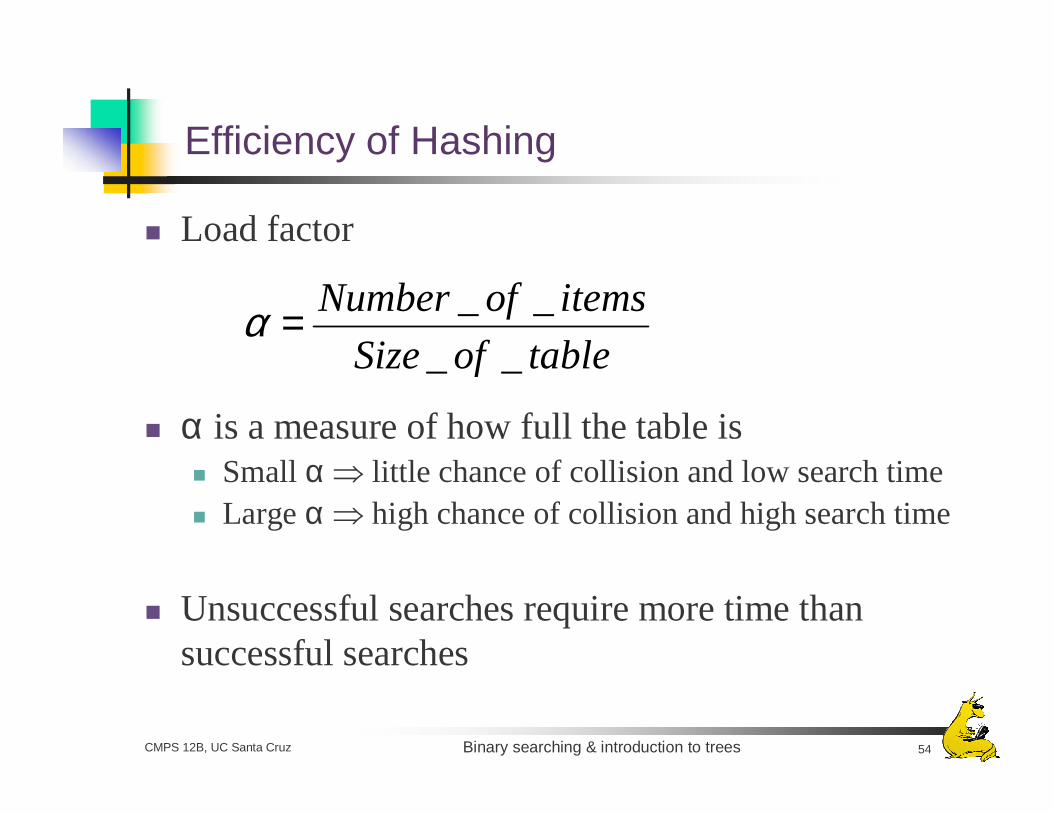
Efficiency of Hashing
Load factor
α is a measure of how full the table isSmall α ⇒ little chance of collision and low search timeLarge α ⇒ high chance of collision and high search time
Unsuccessful searches require more time than successful searches
tableofSize
itemsofNumber
__
__=α
Binary searching & introduction to trees 55CMPS 12B, UC Santa Cruz
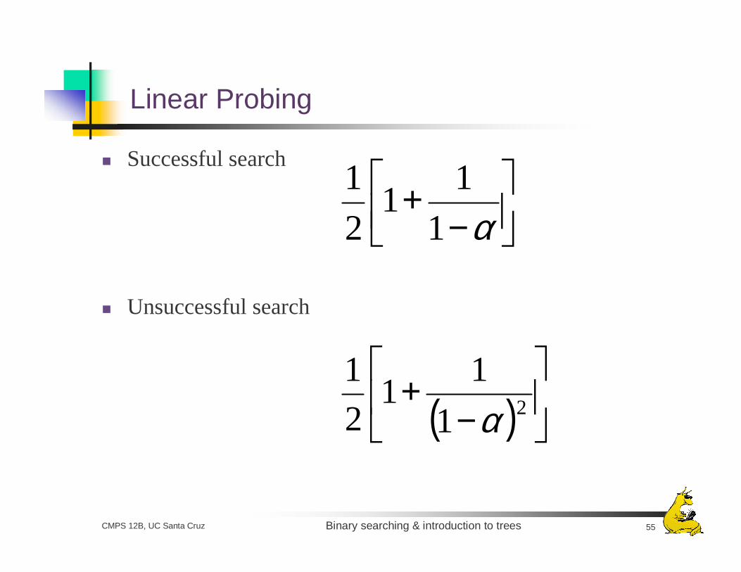
Linear Probing
Successful search
Unsuccessful search
−+
α1
11
2
1
( )
−+ 21
11
2
1
α
Binary searching & introduction to trees 56CMPS 12B, UC Santa Cruz
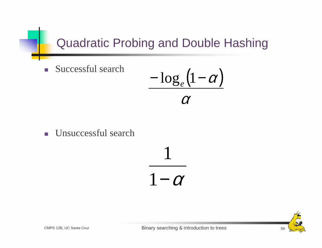
Quadratic Probing and Double Hashing
Successful search
Unsuccessful search
( )α
α−− 1loge
α−1
1
Binary searching & introduction to trees 57CMPS 12B, UC Santa Cruz
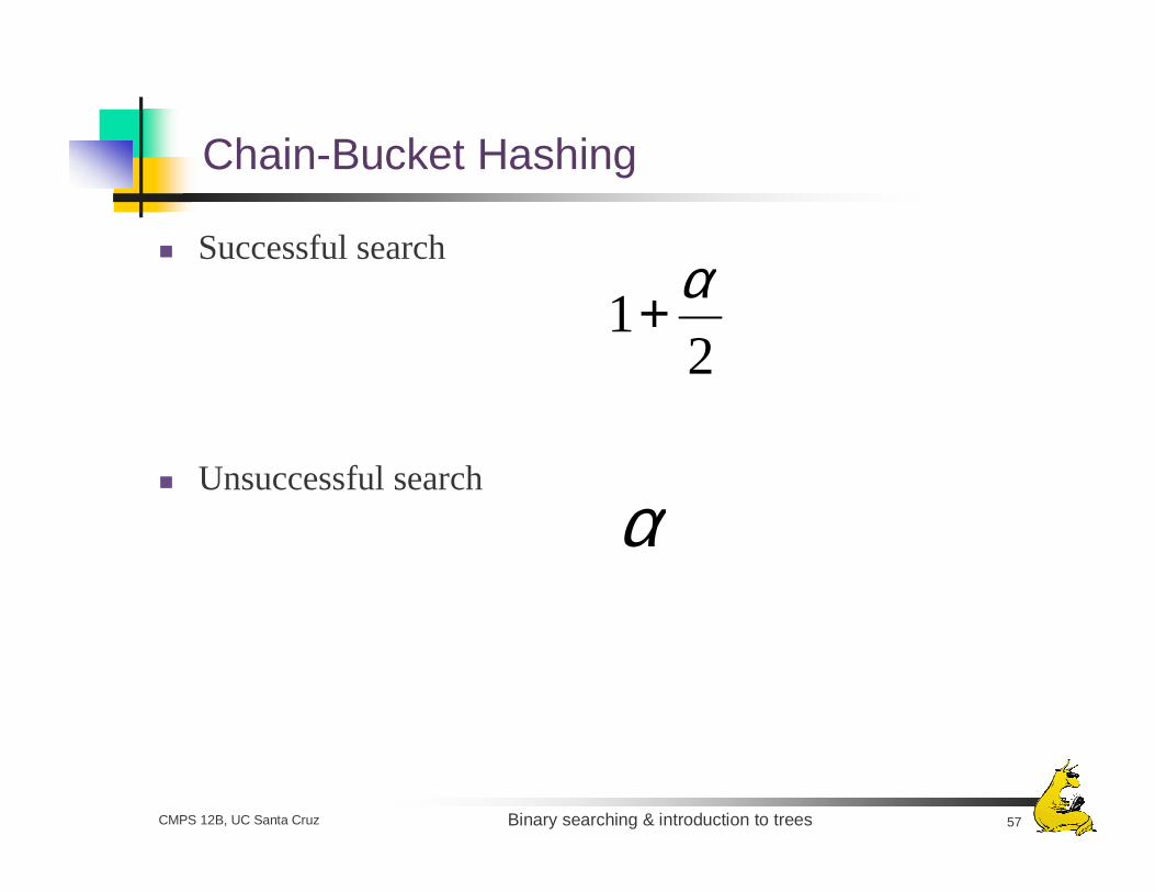
Chain-Bucket Hashing
Successful search
Unsuccessful search
21
α+
α
Binary searching & introduction to trees 58CMPS 12B, UC Santa Cruz
How well does a hash function work?
How fast is it to compute?How well does it scatter random data?How well does it scatter non-random data?
This can be very importantIt is always possible to construct a worst case
General principles:The hash function should involve the whole search keyIf a hash function involves a modulo operation, the base should be prime
Binary searching & introduction to trees 59CMPS 12B, UC Santa Cruz
Hashing vs. Binary Trees
Hashing supports efficient insert and removeHashing does not support efficient sortingHashing does not support efficient range queries