Embed Size (px)
Citation preview
Database Administration
Paper # 524 1
Reviewed by Oracle Certified Master Korea Community
( http://www.ocmkorea.com http://cafe.daum.net/oraclemanager )
AADDVVAANNCCEEDD SSQQLL TTIIPPSS TTHHRROOUUGGHH OORRAACCLLEE 1100GG
INTRODUCTION We will cover advanced SQL concepts, real-world problems and solutions and the performance impact of advanced SQL coding decisions. Ansi-compliant & Oracle 9i and 10g functions and features as well as some creative solutions to SQL problems will be discussed. This will be a fast-paced look at a fun-topic. Some of the things we will look at are:
• Profiling PL/SQL
• 9i/10g Full outer joins and join indexes
• Case and Decode
• 8i and 9i Rankings, Medians
• First and Last Functions
• and more… DBMS_PROFILER: Profiling PL/SQL
• Useful tool to measure PL/SQL performance • Shows performance of lines in a PL/SQL program
o Not just SQL statements. o Can be used to along with tkprof to analyze PL/SQL programs
• Easy to setup and use but: o Many options are available o A lot of data can be produced o Keep the use of it simple
DBMS_Profiler Setup To setup DBMS_Profiler, perform the following steps:
• As user sys create the package o $ORACLE_HOME/rdbms/admin/profload.sql
• As sys or another user (preferred) create tables: o $ORACLE_HOME/rdbms/admin/proftab.sql
• Check profile tables exist (as sys or user): o select count(*) from plsql_profiler_runs; o select count(*) from plsql_profiler_units; o select count(*) from plsql_profiler_data;
If tables setup as SYS, grant the following to public: grant execute on dbms_profiler grant insert,select,update,delete on plsql_profiler_runs
Database Administration
Paper # 524 2
grant insert,select,update,delete on plsql_profiler_units grant insert,select,update,delete on plsql_profiler_data grant all on PLSQL_PROFILER_RUNNUMBER
Create the following public synonyms: plsql_profiler_runs for plsql_profiler_runs; plsql_profiler_units for plsql_profiler_units; plsql_profiler_data for plsql_profiler_data; plsql_profiler_runnumber for plsql_profiler_runnumber
Enhance DBMS_Profiler with tkprof When used along with tkprof, DBMS_Profiler can become even more powerful. Create the following trigger for the user to be traced if you want tkprof to be used to profile the SQL as well: CREATE OR REPLACE TRIGGER user_trace_trigger after logon on database Begin if user=‘username' then execute immediate 'alter session set sql_trace=true'; end if; end; /
List of DBMS_Profiler Functions and Procedures List of the DBMS_Profiler Functions and Procedures (9i,10g)
• Start_Profiler: begin data collection
• Stop_Profiler: stop data collection. Data is not automatically stored when the user disconnects.
• Flush_Data: flush data collected in user session. Can call at points in a run to get incremental data.
• Pause_Profiler: pause user data collection
• Resume_Profiler: resume data collection
• Get_Version (proc): gets the version of this api.
• Internal_Version_Check: verify that the DBMS_Profiler version works with this DB version.
Running Tests with DBMS_Profiler Running Tests: run as the user running PL/SQL: delete from plsql_profiler_data, plsql_profiler_units, plsql_profiler_runs; (and reset input tables)
select * from plsql_profiler_runs; alter session set nls_date_format='YY-MM-DD HH24:MI:SS'; exec dbms_profiler.start_profiler;
Database Administration
Paper # 524 3
select sysdate from dual; exec test_proc; select sysdate from dual; commit; exec dbms_profiler.flush_data; exec dbms_profiler.stop_profiler;
To get the runid from this specific run, query the table plsql_profiler_runs.
select runid, run_owner, run_date from plsql_profiler_runs; • RUNID RUN_OWNER RUN_DATE
1 TESTUSER 02-03-17 22:19:40 Security Points
• Profiler only gathers units for which the user has Create privilege • Oracle advises that modules being profiles should be compiled DEBUG
o rather than NATIVE o can provide extra information about the unit in the database.
DBMS_Profiler Reporting with supplied Packages Oracle provides supplied SQL that can be used for reporting:
• Oracle supplied SQL for reporting o Supplied with oracle 8.x in PL/SQL demo library
• ${ORACLE_HOME}/plsql/demo/profrep.sql o pl/sql profiler utilities and procedures
DBMS_Profiler Reporting on your own Another approach that you can use rather than to use the Oracle supplied packages is to create a temporary table to join the data from the tables that you want to see. An example of this is listed below: create table temp_profiler as select pu.runid, pu.unit_number ,decode(unit_type,'PACKAGE SPEC','PACKAGE',unit_type) unit_type, pu.unit_owner, pu.unit_name, pd.line#, pd.total_occur, pd.total_time, pd.min_time, pd.max_time ,src.text from plsql_profiler_units pu, plsql_profiler_data pd, all_source src where pu.unit_owner = user and pu.unit_name = 'TEST_PROC' and pu.runid=pd.runid and pu.unit_number = pd.unit_number and src.owner = pu.unit_owner and src.type = pu.unit_type and src.name = pu.unit_name and src.line = pd.line#
Database Administration
Paper # 524 4
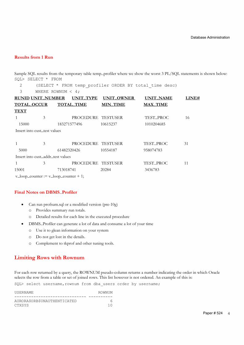
Results from 1 Run Sample SQL results from the temporary table temp_profiler where we show the worst 3 PL/SQL statements is shown below: SQL> SELECT * FROM 2 (SELECT * FROM temp_profiler ORDER BY total_time desc) 3 WHERE ROWNUM < 4;
RUNID UNIT_NUMBER UNIT_TYPE UNIT_OWNER UNIT_NAME LINE#
TOTAL_OCCUR TOTAL_TIME MIN_TIME MAX_TIME
TEXT 1 3 PROCEDURE TESTUSER TEST_PROC 16 15000 183271577496 10615237 1010204685 Insert into cust_test values 1 3 PROCEDURE TESTUSER TEST_PROC 31 5000 61482320426 10554187 958074783 Insert into cust_addr_test values 1 3 PROCEDURE TESTUSER TEST_PROC 11 15001 713018741 20284 3436783 v_loop_counter := v_loop_counter + 1;
Final Notes on DBMS_Profiler
• Can run profsum.sql or a modified version (pre-10g) o Provides summary run totals. o Detailed results for each line in the executed procedure
• DBMS_Profiler can generate a lot of data and consume a lot of your time o Use it to glean information on your system o Do not get lost in the details. o Complement to tkprof and other tuning tools.
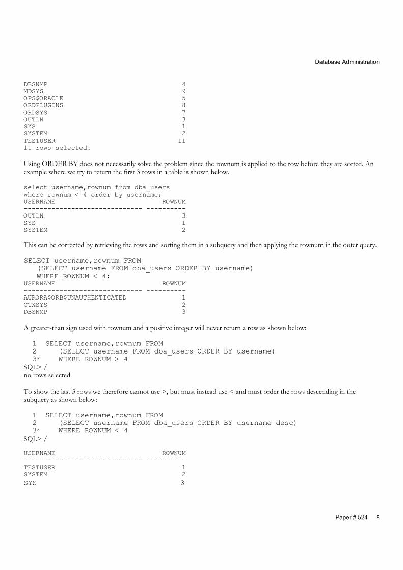
Limiting Rows with Rownum
For each row returned by a query, the ROWNUM pseudo-column returns a number indicating the order in which Oracle selects the row from a table or set of joined rows. This list however is not ordered. An example of this is: SQL> select username,rownum from dba_users order by username; USERNAME ROWNUM ------------------------------ ---------- AURORA$ORB$UNAUTHENTICATED 6 CTXSYS 10
Database Administration
Paper # 524 5
DBSNMP 4 MDSYS 9 OPS$ORACLE 5 ORDPLUGINS 8 ORDSYS 7 OUTLN 3 SYS 1 SYSTEM 2 TESTUSER 11 11 rows selected. Using ORDER BY does not necessarily solve the problem since the rownum is applied to the row before they are sorted. An example where we try to return the first 3 rows in a table is shown below. select username,rownum from dba_users where rownum < 4 order by username; USERNAME ROWNUM ------------------------------ ---------- OUTLN 3 SYS 1 SYSTEM 2 This can be corrected by retrieving the rows and sorting them in a subquery and then applying the rownum in the outer query. SELECT username,rownum FROM (SELECT username FROM dba_users ORDER BY username) WHERE ROWNUM < 4; USERNAME ROWNUM ------------------------------ ---------- AURORA$ORB$UNAUTHENTICATED 1 CTXSYS 2 DBSNMP 3 A greater-than sign used with rownum and a positive integer will never return a row as shown below: 1 SELECT username,rownum FROM 2 (SELECT username FROM dba_users ORDER BY username) 3* WHERE ROWNUM > 4 SQL> / no rows selected To show the last 3 rows we therefore cannot use >, but must instead use < and must order the rows descending in the subquery as shown below: 1 SELECT username,rownum FROM 2 (SELECT username FROM dba_users ORDER BY username desc) 3* WHERE ROWNUM < 4 SQL> / USERNAME ROWNUM ------------------------------ ---------- TESTUSER 1 SYSTEM 2 SYS 3
Database Administration
Paper # 524 6
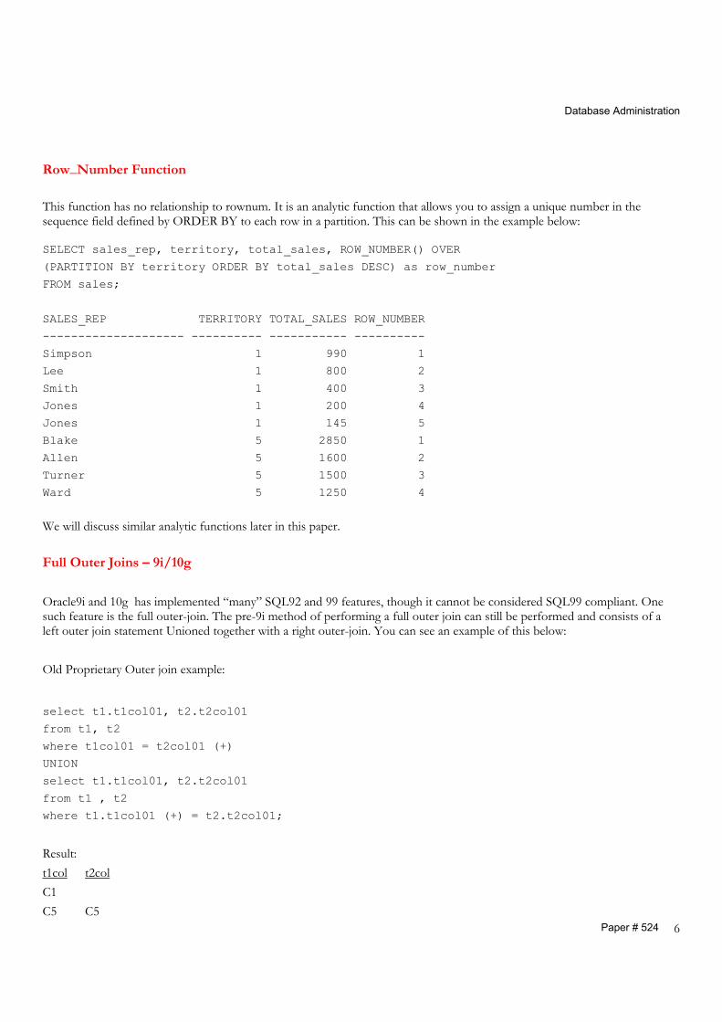
Row_Number Function
This function has no relationship to rownum. It is an analytic function that allows you to assign a unique number in the sequence field defined by ORDER BY to each row in a partition. This can be shown in the example below: SELECT sales_rep, territory, total_sales, ROW_NUMBER() OVER
(PARTITION BY territory ORDER BY total_sales DESC) as row_number
FROM sales;
SALES_REP TERRITORY TOTAL_SALES ROW_NUMBER
-------------------- ---------- ----------- ----------
Simpson 1 990 1
Lee 1 800 2
Smith 1 400 3
Jones 1 200 4
Jones 1 145 5
Blake 5 2850 1
Allen 5 1600 2
Turner 5 1500 3
Ward 5 1250 4
We will discuss similar analytic functions later in this paper. Full Outer Joins – 9i/10g
Oracle9i and 10g has implemented “many” SQL92 and 99 features, though it cannot be considered SQL99 compliant. One such feature is the full outer-join. The pre-9i method of performing a full outer join can still be performed and consists of a left outer join statement Unioned together with a right outer-join. You can see an example of this below: Old Proprietary Outer join example:
select t1.t1col01, t2.t2col01
from t1, t2
where t1col01 = t2col01 (+)
UNION
select t1.t1col01, t2.t2col01
from t1 , t2
where t1.t1col01 (+) = t2.t2col01;
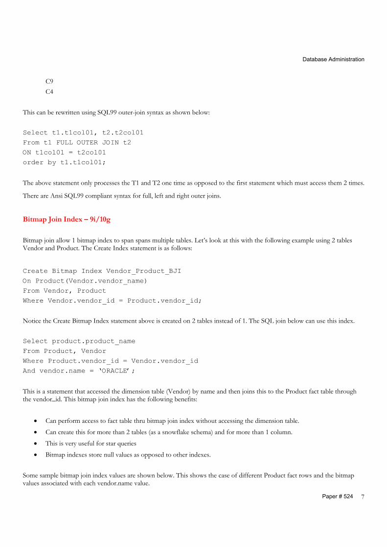
Result: t1col t2col C1 C5 C5
Database Administration
Paper # 524 7
C9 C4 This can be rewritten using SQL99 outer-join syntax as shown below: Select t1.t1col01, t2.t2col01 From t1 FULL OUTER JOIN t2 ON t1col01 = t2col01 order by t1.t1col01;
The above statement only processes the T1 and T2 one time as opposed to the first statement which must access them 2 times.
There are Ansi SQL99 compliant syntax for full, left and right outer joins.
Bitmap Join Index – 9i/10g
Bitmap join allow 1 bitmap index to span spans multiple tables. Let’s look at this with the following example using 2 tables Vendor and Product. The Create Index statement is as follows:
Create Bitmap Index Vendor_Product_BJI On Product(Vendor.vendor_name) From Vendor, Product Where Vendor.vendor_id = Product.vendor_id;
Notice the Create Bitmap Index statement above is created on 2 tables instead of 1. The SQL join below can use this index. Select product.product_name From Product, Vendor Where Product.vendor_id = Vendor.vendor_id And vendor.name = ‘ORACLE’;
This is a statement that accessed the dimension table (Vendor) by name and then joins this to the Product fact table through the vendor_id. This bitmap join index has the following benefits:
• Can perform access to fact table thru bitmap join index without accessing the dimension table.
• Can create this for more than 2 tables (as a snowflake schema) and for more than 1 column.
• This is very useful for star queries
• Bitmap indexes store null values as opposed to other indexes. Some sample bitmap join index values are shown below. This shows the case of different Product fact rows and the bitmap values associated with each vendor.name value.
Database Administration
Paper # 524 8
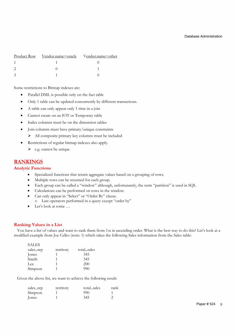
Product Row Vendor.name=oracle Vendor.name=other 1 1 0 2 0 1 3 1 0 Some restrictions to Bitmap indexes are:
• Parallel DML is possible only on the fact table
• Only 1 table can be updated concurrently by different transactions.
• A table can only appear only 1 time in a join
• Cannot create on an IOT or Temporary table
• Index columns must be on the dimension tables
• Join columns must have primary/unique constraints All composite primary key columns must be included
• Restrictions of regular bitmap indexes also apply. e.g. cannot be unique
RANKINGS Analytic Functions
• Specialized functions that return aggregate values based on a grouping of rows. • Multiple rows can be returned for each group. • Each group can be called a “window” although, unfortunately, the term “partition” is used in SQL • Calculations can be performed on rows in the window. • Can only appear in “Select” or “Order By” clause.
o Last operators performed in a query except “order by” • Let’s look at some …
Ranking Values in a List You have a list of values and want to rank them from 1:n in ascending order. What is the best way to do this? Let’s look at a modified example from Joe Celko (note: 1) which takes the following Sales information from the Sales table: SALES sales_rep territory total_sales Jones 1 345 Smith 1 345 Lee 1 200 Simpson 1 990 Given the above list, we want to achieve the following result: sales_rep territory total_sales rank Simpson 1 990 1 Jones 1 345 2
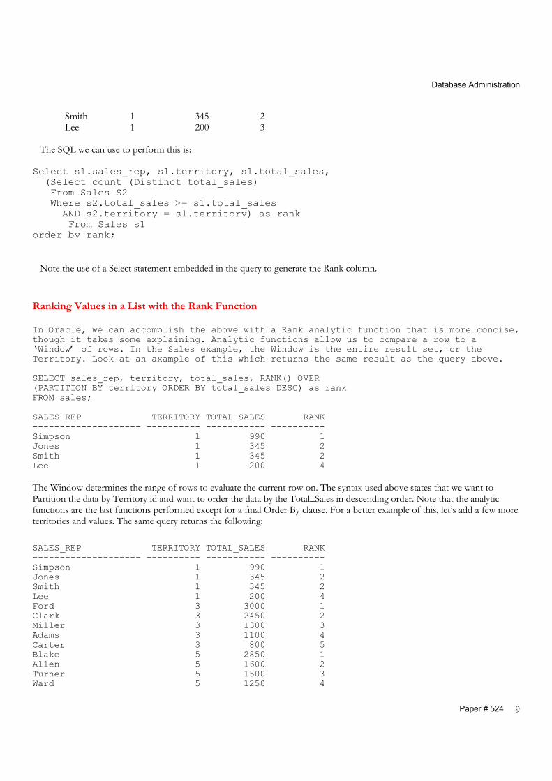
Database Administration
Paper # 524 9
Smith 1 345 2 Lee 1 200 3 The SQL we can use to perform this is: Select s1.sales_rep, s1.territory, s1.total_sales, (Select count (Distinct total_sales) From Sales S2 Where s2.total_sales >= s1.total_sales AND s2.territory = s1.territory) as rank From Sales s1 order by rank; Note the use of a Select statement embedded in the query to generate the Rank column. Ranking Values in a List with the Rank Function In Oracle, we can accomplish the above with a Rank analytic function that is more concise, though it takes some explaining. Analytic functions allow us to compare a row to a ‘Window’ of rows. In the Sales example, the Window is the entire result set, or the Territory. Look at an axample of this which returns the same result as the query above. SELECT sales_rep, territory, total_sales, RANK() OVER (PARTITION BY territory ORDER BY total_sales DESC) as rank FROM sales; SALES_REP TERRITORY TOTAL_SALES RANK -------------------- ---------- ----------- ---------- Simpson 1 990 1 Jones 1 345 2 Smith 1 345 2 Lee 1 200 4 The Window determines the range of rows to evaluate the current row on. The syntax used above states that we want to Partition the data by Territory id and want to order the data by the Total_Sales in descending order. Note that the analytic functions are the last functions performed except for a final Order By clause. For a better example of this, let’s add a few more territories and values. The same query returns the following: SALES_REP TERRITORY TOTAL_SALES RANK -------------------- ---------- ----------- ---------- Simpson 1 990 1 Jones 1 345 2 Smith 1 345 2 Lee 1 200 4 Ford 3 3000 1 Clark 3 2450 2 Miller 3 1300 3 Adams 3 1100 4 Carter 3 800 5 Blake 5 2850 1 Allen 5 1600 2 Turner 5 1500 3 Ward 5 1250 4
Database Administration
Paper # 524 10
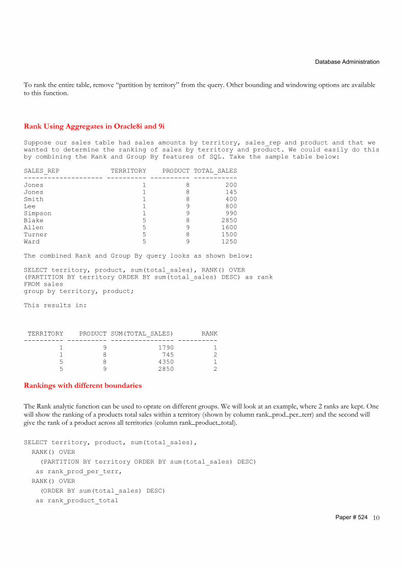
To rank the entire table, remove “partition by territory” from the query. Other bounding and windowing options are available to this function.
Rank Using Aggregates in Oracle8i and 9i Suppose our sales table had sales amounts by territory, sales_rep and product and that we wanted to determine the ranking of sales by territory and product. We could easily do this by combining the Rank and Group By features of SQL. Take the sample table below: SALES_REP TERRITORY PRODUCT TOTAL_SALES -------------------- ---------- ---------- ----------- Jones 1 8 200 Jones 1 8 145 Smith 1 8 400 Lee 1 9 800 Simpson 1 9 990 Blake 5 8 2850 Allen 5 9 1600 Turner 5 8 1500 Ward 5 9 1250 The combined Rank and Group By query looks as shown below: SELECT territory, product, sum(total_sales), RANK() OVER (PARTITION BY territory ORDER BY sum(total_sales) DESC) as rank FROM sales group by territory, product; This results in: TERRITORY PRODUCT SUM(TOTAL_SALES) RANK ---------- ---------- ---------------- ---------- 1 9 1790 1 1 8 745 2 5 8 4350 1 5 9 2850 2
Rankings with different boundaries
The Rank analytic function can be used to oprate on different groups. We will look at an example, where 2 ranks are kept. One will show the ranking of a products total sales within a territory (shown by column rank_prod_per_terr) and the second will give the rank of a product across all territories (column rank_product_total).
SELECT territory, product, sum(total_sales),
RANK() OVER
(PARTITION BY territory ORDER BY sum(total_sales) DESC)
as rank_prod_per_terr,
RANK() OVER
(ORDER BY sum(total_sales) DESC)
as rank_product_total
Database Administration
Paper # 524 11
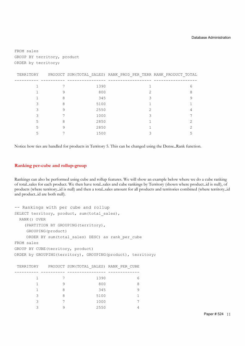
FROM sales
GROUP BY territory, product
ORDER by territory;
TERRITORY PRODUCT SUM(TOTAL_SALES) RANK_PROD_PER_TERR RANK_PRODUCT_TOTAL
---------- ---------- ---------------- ------------------ ------------------
1 7 1390 1 6
1 9 800 2 8
1 8 345 3 9
3 8 5100 1 1
3 9 2550 2 4
3 7 1000 3 7
5 8 2850 1 2
5 9 2850 1 2
5 7 1500 3 5
Notice how ties are handled for products in Territory 5. This can be changed using the Dense_Rank function. Ranking per-cube and rollup-group
Rankings can also be performed using cube and rollup features. We will show an example below where we do a cube ranking of total_sales for each product. We then have total_sales and cube rankings by Territory (shown where product_id is null), of products (where territory_id is null) and then a total_sales amount for all products and territories combined (where territoty_id and product_id are both null). -- Rankings with per cube and rollup SELECT territory, product, sum(total_sales),
RANK() OVER
(PARTITION BY GROUPING(territory),
GROUPING(product)
ORDER BY sum(total_sales) DESC) as rank_per_cube
FROM sales
GROUP BY CUBE(territory, product)
ORDER by GROUPING(territory), GROUPING(product), territory;
TERRITORY PRODUCT SUM(TOTAL_SALES) RANK_PER_CUBE
---------- ---------- ---------------- -------------
1 7 1390 6
1 9 800 8
1 8 345 9
3 8 5100 1
3 7 1000 7
3 9 2550 4
Database Administration
Paper # 524 12
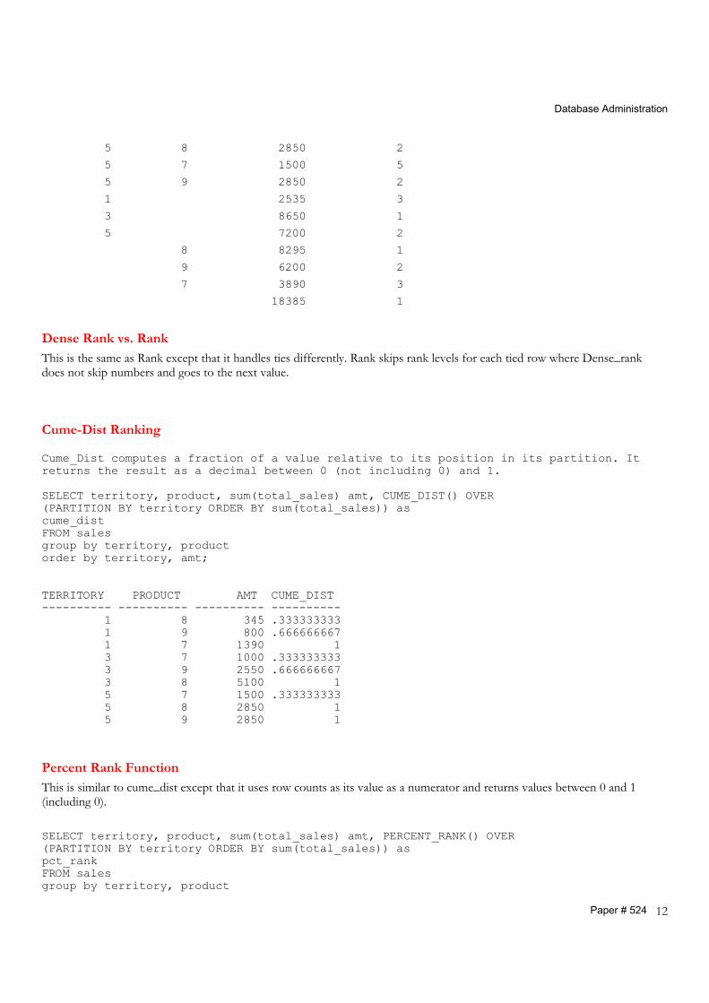
5 8 2850 2
5 7 1500 5
5 9 2850 2
1 2535 3
3 8650 1
5 7200 2
8 8295 1
9 6200 2
7 3890 3
18385 1
Dense Rank vs. Rank
This is the same as Rank except that it handles ties differently. Rank skips rank levels for each tied row where Dense_rank does not skip numbers and goes to the next value. Cume-Dist Ranking Cume_Dist computes a fraction of a value relative to its position in its partition. It returns the result as a decimal between 0 (not including 0) and 1. SELECT territory, product, sum(total_sales) amt, CUME_DIST() OVER (PARTITION BY territory ORDER BY sum(total_sales)) as cume_dist FROM sales group by territory, product order by territory, amt; TERRITORY PRODUCT AMT CUME_DIST ---------- ---------- ---------- ---------- 1 8 345 .333333333 1 9 800 .666666667 1 7 1390 1 3 7 1000 .333333333 3 9 2550 .666666667 3 8 5100 1 5 7 1500 .333333333 5 8 2850 1 5 9 2850 1 Percent Rank Function
This is similar to cume_dist except that it uses row counts as its value as a numerator and returns values between 0 and 1 (including 0). SELECT territory, product, sum(total_sales) amt, PERCENT_RANK() OVER (PARTITION BY territory ORDER BY sum(total_sales)) as pct_rank FROM sales group by territory, product

Database Administration
Paper # 524 13
order by territory, amt / TERRITORY PRODUCT AMT PCT_RANK ---------- ---------- ---------- ---------- 1 8 345 0 1 9 800 .5 1 7 1390 1 3 7 1000 0 3 9 2550 .5 3 8 5100 1 5 7 1500 0 5 8 2850 .5 5 9 2850 .5 Ntile Function Allows you to perform calculations and statistics for tertiles, quartiles, deciles and for other summary statistics. If there are extra rows in buckets, then each bucket will have the same number of rows or at most 1 row more than the others. An example of this is shown below: SELECT sales_rep, total_sales, NTILE(4) OVER (ORDER BY total_sales DESC NULLS FIRST) AS quartile FROM sales ; SALES_REP TOTAL_SALES QUARTILE -------------------- ----------- ---------- Blake 2850 1 Allen 1600 1 Turner 1500 1 Ward 1250 2 Simpson 990 2 Lee 800 3 Smith 400 3 Jones 200 4 Jones 145 4 Hypothetical Rank Analytic functions can be used to determine the rank of a “hypothetical” row inserted into a table.For example, consider a set of product categories that have total_sales determines by sub-category.
• What would the rank of a new product subcategory with sales of $2,000 be?
• What would the rank of a new product subcategory with sales of $1,480 be? Let’s look at an original list of the data and see how the hypothetical rank works with this list.
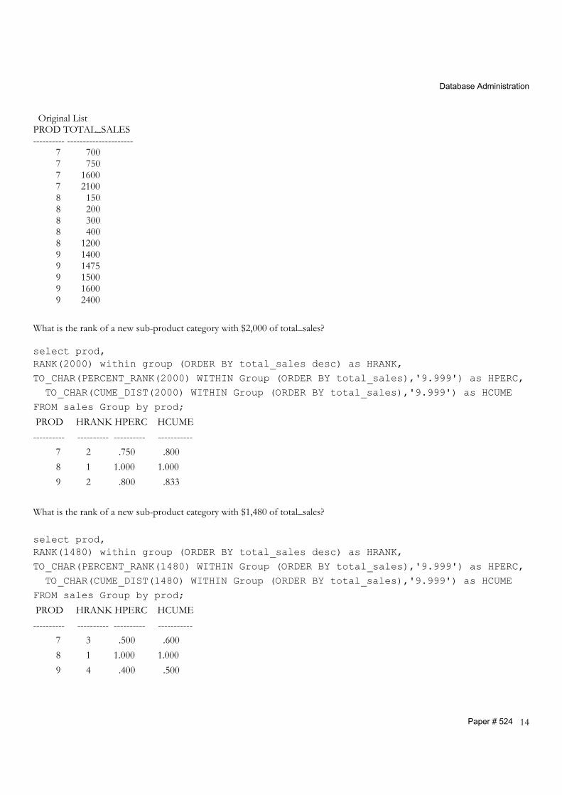
Database Administration
Paper # 524 14
Original List PROD TOTAL_SALES ---------- --------------------- 7 700 7 750 7 1600 7 2100 8 150 8 200 8 300 8 400 8 1200 9 1400 9 1475 9 1500 9 1600 9 2400 What is the rank of a new sub-product category with $2,000 of total_sales? select prod, RANK(2000) within group (ORDER BY total_sales desc) as HRANK, TO_CHAR(PERCENT_RANK(2000) WITHIN Group (ORDER BY total_sales),'9.999') as HPERC, TO_CHAR(CUME_DIST(2000) WITHIN Group (ORDER BY total_sales),'9.999') as HCUME FROM sales Group by prod;
PROD HRANK HPERC HCUME ---------- ---------- ---------- ----------- 7 2 .750 .800 8 1 1.000 1.000 9 2 .800 .833 What is the rank of a new sub-product category with $1,480 of total_sales? select prod, RANK(1480) within group (ORDER BY total_sales desc) as HRANK, TO_CHAR(PERCENT_RANK(1480) WITHIN Group (ORDER BY total_sales),'9.999') as HPERC, TO_CHAR(CUME_DIST(1480) WITHIN Group (ORDER BY total_sales),'9.999') as HCUME FROM sales Group by prod;
PROD HRANK HPERC HCUME ---------- ---------- ---------- ----------- 7 3 .500 .600 8 1 1.000 1.000 9 4 .400 .500
Database Administration
Paper # 524 15
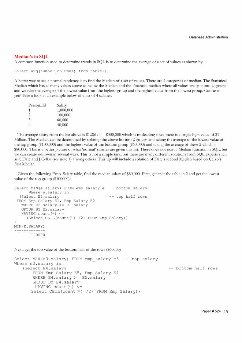
Median’s in SQL A common function used to determine trends in SQL is to determine the average of a set of values as shown by: Select avg(number_column1) from table1; A better way to see a normal tendency is to find the Median of a set of values. There are 2 categories of median. The Statistical Median which has as many values above as below the Median and the Financial median where all values are split into 2 groups and we take the average of the lowest value from the highest group and the highest value from the lowest group. Confused yet? Take a look at an example below of a list of 4 salaries. Person_Id Salary
1 1,000,000 2 100,000 3 60,000 4 40,000
The average salary from the list above is $1.2M/4 = $300,000 which is misleading since there is a single high value of $1 Million. The Median can be determined by splitting the above list into 2 groups and taking the average of the lowest value of the top group ($100,000) and the highest value of the bottom group ($60,000) and taking the average of these 2 which is $80,000. This is a better picture of what ‘normal’ salaries are given this list. There does not exist a Median function in SQL, but we can create our own in several ways. This is not a simple task, but there are many different solutions from SQL experts such as C.Date and J.Celko (see note 1) among others. This tip will include a solution of Date’s second Median based on Celko’s first Median. Given the following Emp_Salary table, find the median salary of $80,000. First, get split the table in 2 and get the lowest value of the top group ($100000): Select MIN(e.salary) FROM emp_salary e -- bottom salary Where e.salary in (Select E2.salary -- top half rows FROM Emp_Salary E1, Emp_Salary E2 WHERE E2.salary <= E1.salary GROUP BY E2.salary HAVING count(*) <= (Select CEIL(count(*) /2) FROM Emp_Salary)) / MIN(E.SALARY) ------------- 100000 Next, get the top value of the bottom half of the rows ($60000) Select MAX(e3.salary) FROM emp_salary e3 -- top salary Where e3.salary in (Select E4.salary -- bottom half rows FROM Emp_Salary E5, Emp_Salary E4 WHERE E4.salary >= E5.salary GROUP BY E4.salary HAVING count(*) <= (Select CEIL(count(*) /2) FROM Emp_Salary))
Database Administration
Paper # 524 16
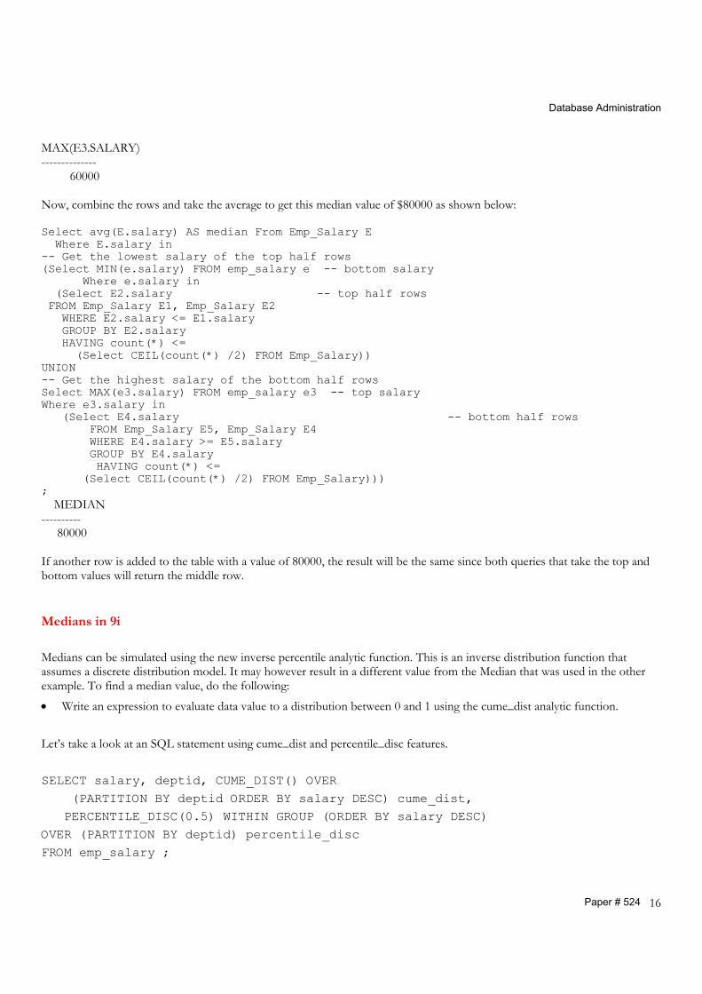
MAX(E3.SALARY) -------------- 60000 Now, combine the rows and take the average to get this median value of $80000 as shown below: Select avg(E.salary) AS median From Emp_Salary E Where E.salary in -- Get the lowest salary of the top half rows (Select MIN(e.salary) FROM emp_salary e -- bottom salary Where e.salary in (Select E2.salary -- top half rows FROM Emp_Salary E1, Emp_Salary E2 WHERE E2.salary <= E1.salary GROUP BY E2.salary HAVING count(*) <= (Select CEIL(count(*) /2) FROM Emp_Salary)) UNION -- Get the highest salary of the bottom half rows Select MAX(e3.salary) FROM emp_salary e3 -- top salary Where e3.salary in (Select E4.salary -- bottom half rows FROM Emp_Salary E5, Emp_Salary E4 WHERE E4.salary >= E5.salary GROUP BY E4.salary HAVING count(*) <= (Select CEIL(count(*) /2) FROM Emp_Salary))) ; MEDIAN ---------- 80000 If another row is added to the table with a value of 80000, the result will be the same since both queries that take the top and bottom values will return the middle row. Medians in 9i Medians can be simulated using the new inverse percentile analytic function. This is an inverse distribution function that assumes a discrete distribution model. It may however result in a different value from the Median that was used in the other example. To find a median value, do the following:
• Write an expression to evaluate data value to a distribution between 0 and 1 using the cume_dist analytic function. Let’s take a look at an SQL statement using cume_dist and percentile_disc features. SELECT salary, deptid, CUME_DIST() OVER (PARTITION BY deptid ORDER BY salary DESC) cume_dist, PERCENTILE_DISC(0.5) WITHIN GROUP (ORDER BY salary DESC) OVER (PARTITION BY deptid) percentile_disc FROM emp_salary ;
Database Administration
Paper # 524 17
salary deptid cume_dist percentile_dist 1000000 100 .25 100000 100000 100 .5 100000 60000 100 .75 100000 40000 100 1 100000 Using the above, the inverse percentile finds the value at the 0.5 cume_dist level.
In the example this is 100,000 Using 0.51 would have given 60,000
This may not be the Median you are looking for but you can see how this can be used in some cases to find the Median value.
Medians in 10g Finally, a Median function!
• Inverse distribution function assuming continuous distribution.
• Null values are ignored.
• Numeric datatypes and nonnumeric ones con be converted to numeric.
• Median first orders the rows.
• With N as the number of rows, Oracle determines the median row number (MRN) as: MRN = 1 + (0.5*(N-1))
• Once Oracle has determined the MRN, it gets ceiling row number (CRN) and floor row number (FRN) and uses these to get the Median.
CRN=ceiling(RN) and FRN = floor(RN) If (CRN=FRN=RN) then median = RN_value Else Median = (CRN-RN) * (FRN_value)
+ (RN-FRN) * (CRN_value) Select region, median(dollar_sales) From Sales_Hist Group By region;
HISTOGRAMS: What Are They? Oracle uses histogram statistics to evaluate the optimal query optimization using a feature called Histograms. A histogram can be used on a column to specify how data is skewed. The histogram will contain a number of buckets with counts of the number or rows that exist for that bucket, or with column values that exist in a certain section of the Table. For example, if there are 10 buckets and 100,000 rows in a Table, these could each represent 10% of the Table. The first bucket could state how many rows are in the first 10% of the key range, while the second could state the number of rows in the second 10% of the key range and so on. Another approach would be to state column_value at the 10% mark, then the column value at the 20% mark and so on. Whichever approach is used, the Histogram is a very useful tool for determining “data skewing” and should be considered for indexed columns that do not have an even distribution. Look for this feature in your database and

Database Administration
Paper # 524 18
remember that the greater the number of buckets in your Histogram, the greater the degree of accuracy your Database Optimizer will have. Oracle splits the data into bands. These can be height-based or value-based and Oracle generally uses a height-based approach but will sometimes use frequency-based histograms. Height-based histograms place column values into the number of buckets specified in the histogram statement. If we specify 10 buckets, then Oracle divides the table into 10 equal parts and places the value of the column at that place in the table. So, in a skewed table, the value may look like this: |-----|--------|--------|----------|-------|-------|--------|------|--------| 1 3 3 1000 3000 3010 3010 7000 8000 40000 The above histogram tells the Oracle that only 10% of the values for this column are > 8000 and that 90% are <= 8000. When considering whether to use Histograms, keep the following points in mind: - Create histograms for columns that are indexed or frequently queried and have skewed data. - Histograms are not useful if predicates on the column use bind variables, data id evenly distributed or data is unique and
always used with an = predicate. - Histograms can be created using the DBMS_STATS package or with the analyze statement. - The default number of histogram buckets is 75 minimum is 1 and maximum is 254. A sample analyze for a table that has 110 rows and 10 sample buckets is shown below: analyze table testtq compute statistics for all columns size 10;
- or optionally - EXECUTE DBMS_STATS.GATHER_TABLE_STATS ('system','testtq', METHOD_OPT => 'FOR COLUMNS SIZE 10 col01'); To view information on histograms, you can view the following tables: All|DBA|USER_histograms, All|DBA|USER_part_histograms, All|DBA|USER_subpart_histograms, All|DBA|USER_tab_columns, ALL|DBA|USER_tab_col_statistics. You can view DBA_HISTOGRAMS for the number of buckets (number of rows for each Column). Examples of the DBA_Histograms and all_tab_col_statistics tables from the analyze above are shown here: Select endpoint_number, endpoint_value From dba_histograms Where table_name = 'TESTTQ' and column_name = 'COL03'; ENDPOINT_NUMBER ENDPOINT_VALUE -------------------------------- -------------------------------------- 0 0 1 10 2 14 3 36 4 42 5 54 6 77 7 200 8 201
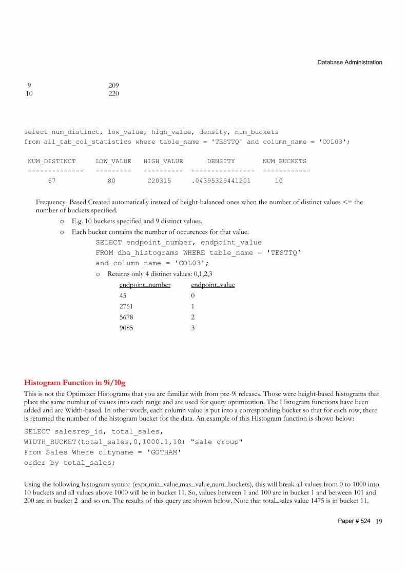
Database Administration
Paper # 524 19
9 209 10 220 select num_distinct, low_value, high_value, density, num_buckets
from all_tab_col_statistics where table_name = 'TESTTQ' and column_name = 'COL03';
NUM_DISTINCT LOW_VALUE HIGH_VALUE DENSITY NUM_BUCKETS
-------------- --------- ---------- ---------------- ------------
67 80 C20315 .04395329441201 10
Frequency- Based Created automatically instead of height-balanced ones when the number of distinct values <= the number of buckets specified.
o E.g. 10 buckets specified and 9 distinct values. o Each bucket contains the number of occurences for that value.
SELECT endpoint_number, endpoint_value FROM dba_histograms WHERE table_name = 'TESTTQ‘ and column_name = 'COL03';
o Returns only 4 distinct values: 0,1,2,3 endpoint_number endpoint_value 45 0 2761 1 5678 2 9085 3
Histogram Function in 9i/10g This is not the Optimizer Histograms that you are familiar with from pre-9i releases. Those were height-based histograms that place the same number of values into each range and are used for query optimization. The Histogram functions have been added and are Width-based. In other words, each column value is put into a corresponding bucket so that for each row, there is returned the number of the histogram bucket for the data. An example of this Histogram function is shown below:
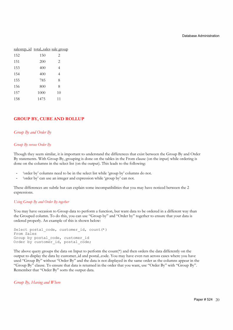
SELECT salesrep_id, total_sales, WIDTH_BUCKET(total_sales,0,1000.1,10) “sale group" From Sales Where cityname = 'GOTHAM' order by total_sales;
Using the following histogram syntax: (expr,min_value,max_value,num_buckets), this will break all values from 0 to 1000 into 10 buckets and all values above 1000 will be in bucket 11. So, values between 1 and 100 are in bucket 1 and between 101 and 200 are in bucket 2 and so on. The results of this query are shown below. Note that total_sales value 1475 is in bucket 11.
Database Administration
Paper # 524 20
salesrep_id total_sales sale group 152 150 2 151 200 2 153 400 4 154 400 4 155 785 8 156 800 8 157 1000 10 158 1475 11
GROUP BY, CUBE AND ROLLUP
Group By and Order By Group By versus Order By Though they seem similar, it is important to understand the differences that exist between the Group By and Order By statements. With Group By, grouping is done on the tables in the From clause (on the input) while ordering is done on the columns in the select list (on the output). This leads to the following: - ‘order by’ columns need to be in the select list while ‘group by’ columns do not. - ‘order by’ can use an integer and expression while ‘group by’ can not.
These differences are subtle but can explain some incompatibilities that you may have noticed between the 2 expressions. Using Group By and Order By together You may have occasion to Group data to perform a function, but want data to be ordered in a different way than the Grouped column. To do this, you can use “Group by” and “Order by” together to ensure that your data is ordered properly. An example of this is shown below: Select postal_code, customer_id, count(*) From Sales Group by postal_code, customer_id Order by customer_id, postal_code; The above query groups the data on Input to perform the count(*) and then orders the data differently on the output to display the data by customer_id and postal_code. You may have even run across cases where you have used “Group By” without “Order By” and the data is not displayed in the same order as the columns appear in the “Group By” clause. To ensure that data is returned in the order that you want, use “Order By” with “Group By”. Remember that “Order By” sorts the output data. Group By, Having and Where
Database Administration
Paper # 524 21
SQL statements that have a Group By clause may have data filtered by a Where clause and by a Having clause. The Having clause filters data after the Group by aggregation while the Where clause filters it before the 'Group By' is performed. It is more efficient to eliminate rows in a Where clause when possible. An example of such a statement is: Select owner, sum(num_rows)
From all_tables Where num_rows > 10000 Group by owner Having sum(num_rows) > 1000000;
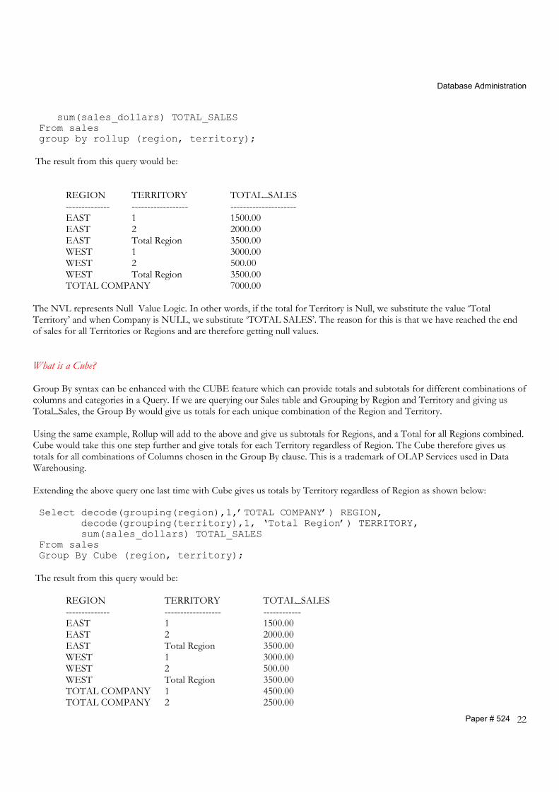
The above statement sums the number of rows for all tables that have more than 10,000 rows and displays those owners that have more than 1,000,000 rows combined. The filtering for 10,000 rows is performed first for each owner then the Group By is performed on only those tables with > 10,000 rows, then each owner is checked to see if the remaining tables have > 1,000,000 row. Extending Group By Group By can allow aggregates to be performed on a single column or on a set of columns. It is a powerful, but simple feature of SQL. “Group By” alone however does not provide us with all of the Grouping information that we may want to have. There are 2 other features that may be used to enhance Group By. These are Cube and Rollup. Rollup can be used to extend Group By to aggregate at many levels, including the Grand Total. Cube can further extend Rollup by calculating all possible combinations of subtotals for a Group By. It makes cross-tab reports possible for Group By columns. Group By with Rollup It is simple to Group By a set of columns and to perform a Sum function based on this grouping. An example of this groups by Sales Region and Territory as follows: Select region, territory, sum(sales_dollars) TOTAL_SALES From sales group by region, territory; The result from this query is:
REGION TERRITORY TOTAL_SALES ------------- ----------------- ---------------------
EAST 1 1500.00 EAST 2 2000.00 WEST 1 3000.00 WEST 2 500.00 What if we want the above and we want to also summarize at the Region level and for the Entire Result set. To do this required the ROLLUP function. It can be used as follows: Select nvl(region,’TOTAL COMPANY’) REGION, nvl(territory, ‘Total Region’) TERRITORY,
Database Administration
Paper # 524 22
sum(sales_dollars) TOTAL_SALES From sales group by rollup (region, territory); The result from this query would be:
REGION TERRITORY TOTAL_SALES -------------- ------------------ ---------------------
EAST 1 1500.00 EAST 2 2000.00 EAST Total Region 3500.00 WEST 1 3000.00 WEST 2 500.00 WEST Total Region 3500.00 TOTAL COMPANY 7000.00 The NVL represents Null Value Logic. In other words, if the total for Territory is Null, we substitute the value ‘Total Territory’ and when Company is NULL, we substitute ‘TOTAL SALES’. The reason for this is that we have reached the end of sales for all Territories or Regions and are therefore getting null values. What is a Cube? Group By syntax can be enhanced with the CUBE feature which can provide totals and subtotals for different combinations of columns and categories in a Query. If we are querying our Sales table and Grouping by Region and Territory and giving us Total_Sales, the Group By would give us totals for each unique combination of the Region and Territory. Using the same example, Rollup will add to the above and give us subtotals for Regions, and a Total for all Regions combined. Cube would take this one step further and give totals for each Territory regardless of Region. The Cube therefore gives us totals for all combinations of Columns chosen in the Group By clause. This is a trademark of OLAP Services used in Data Warehousing. Extending the above query one last time with Cube gives us totals by Territory regardless of Region as shown below: Select decode(grouping(region),1,’TOTAL COMPANY’) REGION, decode(grouping(territory),1, ‘Total Region’) TERRITORY, sum(sales_dollars) TOTAL_SALES From sales Group By Cube (region, territory); The result from this query would be:
REGION TERRITORY TOTAL_SALES -------------- ------------------ ------------
EAST 1 1500.00 EAST 2 2000.00 EAST Total Region 3500.00 WEST 1 3000.00 WEST 2 500.00 WEST Total Region 3500.00 TOTAL COMPANY 1 4500.00 TOTAL COMPANY 2 2500.00
Database Administration
Paper # 524 23
TOTAL COMPANY Total Region 7000.00 The decode function is a translation in Oracle that changes the grouping indicator of ‘1’ into another value of ‘TOTAL COMPANY’ or ‘Total Region’. Dealing with Nulls in CUBE and Rollup You may have noticed with CUBE and ROLLUP that we check for NULL values to be returned to determine that a higher level summary (rollup) has been reached. There is a catch to this: what if the value returned by a higher level such as at the Territory level (using our example) actually is NULL? How do we distinguish that the NULL is returned by the query or by a ROLLUP? Rollup and Cube provides a facility where a value of 1 is returned if the NULL is a result of CUBE or ROLLUP and it returns 0 if it is a natural result. To take advantage of this in Oracle, write the query as follows: Select decode(grouping(region),1,’TOTAL COMPANY’) REGION, decode(grouping(territory),1, ‘Total Region’) TERRITORY, sum(sales_dollars) TOTAL_SALES From sales group by rollup (region, territory); The decode function translates the grouping indicator of ‘1’ into another value of ‘TOTAL COMPANY’ or ‘Total Region’. Grouping Sets – 9i/10g
This new 9i feature enhances SQL groupings used by the Cube and Rollup Group By clauses. Grouping Sets allows us to specify the exact level of aggregation across various combinations of columns. Let’s look at an example of a set of aggregations across 3 different groupings. To do this with a Cube would require many groupings and a “Union All” would use 3 queries. Consider the input data listed below.
month prod terr total_sales 1 1 8 200 2 1 8 150 1 2 8 300 2 2 8 400 1 1 9 1400 2 1 9 1600 1 2 9 1500 2 2 9 1475 We want to provide 3 sets of groupings by:
1) month, terr, prod. 2) month, prod. 3) terr, prod. This can be accomplished with the following SQL (note the “Group By Grouping Sets” syntax): Select month, terr, prod,
Database Administration
Paper # 524 24
sum(total_sales) sum_sales From sales Group By Grouping Sets ((month, terr, prod), (month, prod), (terr, prod));
The result of this is below: month terr prod sum_sales 1 1 8 200 1 2 8 300 1 1 9 1400 1 2 9 1500 2 1 8 150 2 2 8 400 2 1 9 1600 2 2 9 1475 1 8 500 1 9 2900 2 8 550 2 9 3075 1 8 350 1 9 3000 2 8 700 2 9 2975 MERGE The Merge statement is not a merge-join. It can be used to update or delete on the target table if the row exists, otherwise insert into the table. This can be used to update-only or insert-only. An update can delete rows based on a condition and conditional logic can be applied through Where clauses. An example of this is shown below. Merge into target_table t1 Using source_table s1 ON (t1_id=s1_id) WHEN Matched Then Update Set t1.col2 = s1.col2 Delete where (t1.delete_flag = ‘Y’) WHEN NOT Matched Then Insert(t1.t1_id,t1.col2) Values (s1.s1_id,s1.col2);
Database Administration
Paper # 524 25
Advantages of the Merge statement are: • For simple Insert/Update, more simple SQL
• Fewer source scans needed
• Fewer statements executed Disadvantages of Merge are:
• Only use for simple logic.
Lead/Lag Analytic Function This analytic function provides us with the capability to determine the next value in a list without performing a self-join. Though this is not the same as traversing a tree or bill-of-materials type of structure it has great benefits in helping us find the next row without needing to code a subquery – though the syntax may be even more difficult to understand than subquery logic is. Let’s take the example of a table employee with columns ename and hiredate. Suppose that we want to develop a query where each row has the employees name, their hiredate and the next employees hire date. This could be accomplished through a join to a subquery that retrieves the lowest hiredate that is larger than the one on this row. Or, more simply, we can use the Lead function as follows: SELECT ename, hiredate, LEAD(hiredate, 1) OVER (ORDER BY hiredate) AS next_hire_date FROM employee; ENAME HIREDATE NEXT_HIRE_DATE --------------- ----------- -------------- COHEN 1991-APR-01 1991-OCT-31 KING 1991-OCT-31 1992-JAN-10 LEE 1992-JAN-10 1992-FEB-12 ALLEN 1992-FEB-12 1995-NOV-25 JONES 1995-NOV-25 1999-DEC-15 SMITH 1999-DEC-15 The offset of 1 tells Oracle to find the next row. If you do not specify offset, its default is 1. To retrieve the date of the employee hired before the employee on a row, use the LAG analytic function: SELECT ename, hiredate, LAG(hiredate, 1) OVER (ORDER BY hiredate) AS prev_hire_date FROM employee SQL> / ENAME HIREDATE PREV_HIRE_DATE --------------- ----------- -------------- COHEN 1991-APR-01 KING 1991-OCT-31 1991-APR-01 LEE 1992-JAN-10 1991-OCT-31 ALLEN 1992-FEB-12 1992-JAN-10 JONES 1995-NOV-25 1992-FEB-12 SMITH 1999-DEC-15 1995-NOV-25 This can be very useful for determining things like effective and expiry dates on a row where only 1 date exists. CASE Case Expression This is a very powerful statement that allows you to add If…Then…Else logic to your SQL. Select a result and return it.
Database Administration
Paper # 524 26
• Without adding procedural logic
• More powerful than decode
• Search is for the first condition that matches and falls through to Else condition or returns Null.
• Simple case available in 8i
• Searched Case in 9i and 10g
• Nullif in 9i and 10g
• Coalesce in 9i and 10g
Case - Simple The simple format of the Case statement can be thought of as being similar to Decode logic Select (CASE region_code WHEN ‘A’ THEN ‘East’ WHEN ‘B’ THEN ‘West’ ELSE ‘Other’ END) As ‘Region’ from region_tbl;
Case Search/Replace Values can be searched for and replaces with the Case statement. For example: Select last_name, (CASE WHEN ‘A%’ THEN ‘1’ WHEN ‘B%’ THEN ‘2’ WHEN ‘C%’ THEN ‘3’ ELSE ‘4’ END) as ‘Name_Group’ From Employees;
Case and Nullif Nullif returns null if the first argument equals the second. If not, the first argument is returned. Example Nullif (expression1,expression2) - is the same as - Case When expression1 = expression2 Then Null Else expression1 End
Database Administration
Paper # 524 27
Case and Coalesce Coalesce is similar to NVL. It allows you to search a number of arguments and returns the first one that is not-null. If all are null, then returns null Example Coalesce(arg1,arg2,arg3) - is the same as - Case When arg1 is not null THEN arg1 When arg2 is not null THEN arg2 ELSE arg3 END
Case Statement Similar to Case Expression BUT each WHEN clause can be a PL/SQL block Example
[<<label_name>>] CASE selector WHEN expression1 THEN many_statements1; WHEN expressionN THEN
stored_proc1; stored_proc2;
ELSE many_statementsN+1;] END CASE [label_name];
Note the label clause that can be used. First/Last Functions The First/Last Functions are analytic, aggregate functions that operate on a set of values from a set of rows. Use these when you need the lowest or highest value from a sorted set to compare to another value from a function such as min, max, sum,avg, count. Let’s look at an example to find the max salary of employees who have received the highest bonus and to find the lowest salary of employees who have received the lowest bonus.
The Input Data is shown below: salary deptid bonus 1,000,000 100 20,000 100,000 100 20,000 60,000 100 15,000 40,000 100 15,000
Database Administration
Paper # 524 28
SELECT deptid, min(salary) keep (dense_rank FIRST order by bonus) "low", max(salary) keep (dense_rank LAST order by bonus) "high", FROM emp_salary group by deptid;
The Result is Below: deptid low high 100 40000 1000000 In other words, the lowest salary that received the lowest bonus of 15,000 was 40,000 and the highest salary that received the highest bonus of 20,000 was 1000000. Correlated Updates: Updating 1 column from a value on another row. This seems like a simple task, but is complicated and can lead to corrupted data if not performed very carefully. Given 2 tables, we want to update a column on 1 table with values from another. Assume that we have 2 tables, Table1 and Table2 as shown below: SQL> select * from table1 order by t1_id; T1_ID T1_C1 T1_C2 ---------- ----- ----- 1 A AAA 2 B BBB 3 C CCC 4 D DDD SQL> select * from table2 order by t2_id; T2_ID T2_C1 T2_C2 ---------- ----- ----- 2 W WWW 4 X XXX 6 Y YYY 8 Z ZZZ We want to update the column named t1_c1 on table TABLE1 with values from column t2_c1 on table TABLE2 where the keys are the same. It would appear at first glance that the following query would produce the results that we want: SQL> Update table1 a 2 Set a.t1_c1 = (select b.t2_c1 from table2 b 3 where b.t2_id = a.t1_id) 4 / 4 rows updated. But, upon further inspection we see that all values for t1_c1 were updated as follows: SQL> select * from table1 order by t1_id;
Database Administration
Paper # 524 29
T1_ID T1_C1 T1_C2 ---------- ----- ----- 1 AAA 2 W BBB 3 CCC 4 X DDD Our matching on t1_id = t2_id worked to read the new matching values ‘W’ and ‘X’, but they did not update the correct rows on table TABLE1. We need to enhance this query as follows: SQL> Update table1 a 2 Set a.t1_c1 = (select b.t2_c1 from table2 b 3 where b.t2_id = a.t1_id) 4 Where a.t1_id = (select t2_id from table2 5 where t2_id = a.t1_id); 2 rows updated. SQL> SQL> select * from table1 order by t1_id; T1_ID T1_C1 T1_C2 ---------- ----- ----- 1 A AAA 2 W BBB 3 C CCC 4 X DDD We needed 2 subqueries: one to pick up the values that we wanted and another to apply these to the correct rows on the outer table. Always check your results when performing correlated updates. Check the results before committing and backup your data before performing this operation. COMPARING JOIN TECHNIQUES Merge Scan joins, Nested-Loop joins, Hash Joins and Star queries. Nested Loop Joins The Nested Loop join is one of the 2 most common join techiniques - the other being the Sort Merge join. This is also a relatively simple join to understand. Take the example of 2 tables joined as follows: Select * From Table1 T1, Table2 T2 Where T1.Table1_Id = T2.Table1_id;
In the case of the Nested Loop Join, the rows will be accessed with an outer table being chosen (say Table1 in this case) and for each row in the outer table, the inner table (Table2) will be accessed with an index to retrieve the matching rows. Once all matching rows from Table2 are found, then the next row on Table1 is retrieved and the matching to Table2 is performed again.
Database Administration
Paper # 524 30
It's important that efficient index access is used on the inner table (Table2 in this example) or that the inner table be a very small table. This is critical to prevent table scans from being performed on the inner table for each row of the outer table that was retrieved. Nested Loop joins are usually used in cases where relatively few rows are being accessed in the outer table and joined to the inner table using efficient index access. It is the most common join performed by transactional (OLTP) systems. Cluster Joins are a special case of Nested-Loop join where the outer table can access the inner table with the cluster index. Clusters can be very efficient, but have many maintenance and performance drawbacks. These are rarely used. Sort-Merge Joins The Sort-Merge join - also called a Merge Scan - is a very popular join performed when accessing a large number of rows. It is also seen in background tasks, batch processing and decision support systems. Take an example of 2 tables being joined and returning a large number of rows (say, thousands) as follows: Select * From Table1 T1, Table2 T2 Where T1.Table1_Id = T2.Table1_id;
The Merge Scan join will be chosen because the database has detected that a large number of rows need to be processed and it may also notice that index access to the rows are not efficient since the data is not clustered (ordered) efficiently for this join. The steps followed to perform this type of join are as follows: 1) Pick an inner and outer table 2) Access the inner table, choose the rows that match the predicates in the Where clause of the SQL statement. 3) Sort the rows retrieved from the inner table by the joining columns and store these as a Temporary table. This step may not be performed if data is ordered by the keys and efficient index access can be performed. 4) The outer table may also need to be sorted by the joining columns so that both tables to be joined are sorted in the same manner. This step is also optional and dependent on whether the outer table is already well ordered by the keys and whether efficient index access can be used. 5) Read both outer and inner tables (these may be the sorted temporary tables created in previous steps), choosing rows that match the join criteria. This operation is very quick since both tables are sorted in the same manner and Database Prefetch can be used. 6) Optionally sort the data one more time if a Sort was performed (e.g. an 'Order By' clause) using columns that are not the same as were used to perform the join. The Merge Join can be deceivingly fast due to database multi-block fetch (helped by initialization parameter db_file_multiblock_read_count) capabilities and the fact that each table is accessed only one time each. These are only used for equi-joins. The other init.ora parm that can be tuned to help performance is sort_area_size. Hash Join The Hash Join is is a very efficient join when used in the right situation. With the hash join, one Table is chosen as the Outer table. This is the larger of the two tables in the Join - and the other is chosen as the Inner Table. Both tables are broken into
Database Administration
Paper # 524 31
sections and the inner Tables join columns are stored in memory (if hash_area_size is large enough) and 'hashed'. This hashing provides an algorithmic pointer that makes data access very efficient. Oracle attempts to keep the inner table in memory since it will be 'scanned' many times. The Outer rows that match the query predicates are then selected and for each Outer table row chosen, hashing is performed on the key and the hash value is used to quickly find the matching row in the Inner Table. This join can often outperform a Sort Merge join, particularly when 1 table is much larger than another. No sorting is performed and index access can be avoided since the hash algorithm is used to locate the block where the inner row is stored. Hash-joins are also only used for equi-joins. Other important init.ora parms are: hash_join_enabled, sort_area_size and hash_multiblock_io_count. Star Joins A particular type of join common to Data Marts and Data Warehouses is known as the "star-join" or "star-query". This is a join of a large "Fact" table with 2 or more smaller tables commonly called "Dimensions". Fact tables may be thought of as having transactional properties. An example of a Fact table is Sales which contains keys and some measures. This is commonly a large table with millions - and sometimes billions - of rows. The Dimensional tables are used to describe the Fact table. Examples of Dimension tables are: Customer, Product and Time. Star queries get their name because there is a single Fact table in the middle and the smaller dimensional tables are directly related to the Fact table. To explain how Star-Joins work, let’s consider an example of a central Fact table and 3 small Dimensional tables related to the Fact table. The first and most simple approach for resolving a star-query is to query the 3 dimensional tables using the predicates in the Where clause to filter out unnecessary rows. The resulting rows from the 3 dimension tables can be joined together forming a cartesian product. This is not as bad as it sounds since these tables are relatively small and the rows matching the 'Where' criteria account for a subset of these. This cartesian product can be sorted and stored as a temporary table. A merge-scan join can then be performed between the resulting temporary table and the Fact table. There is a more complex approach that the Database optimizer can take towards Star Joins that is used in Oracle8i. Consider the case of the central Fact table that is being joined to 3 smaller Dimensional tables as shown below: Select * From Fact, Dim1, Dim2, Dim3 Where Fact.dim1_id = Dim1.id and Fact.dim2_id = Dim2.id and Fact.dim3_id = Dim3.id and Dim1.name like :input_variable_name and Dim2.Descriprion between :input_var1 and :input_var2 and Dim3.Text < :input_variable_text;
The optimizer can transform this by adding 3 subqueries so that the new transformed query looks like this: Select * From Fact, Dim1, Dim2, Dim3 Where Fact.dim1_id in (Select dim1.id from dim1 where dim1.name like :input_variable_name) and Fact.dim2_id in (Select dim2.id from dim2 where Dim2.descriprion between :input_var1 and :input_var2)
Database Administration
Paper # 524 32
and Fact.dim3_id in (Select dim3.id from dim3 where Dim3.Text < :input_variable_text);
Given the above, the subselects are performed first. If bitmap indexes exist on the Fact join columns, then the bitmap index entries that result from each subquery can be merged (in this case ANDed) together and the Fact table data can be retreived using the resulting index values. This is a very quick operation. The Fact entries retrieved can then be joined to the Dimension tables to complete the query. Using this approach, a Cartesian product is not required. To implement star_query transformation:
• Set init.ora parm star_transformation_enabled
• Create bitmap indexes for all of the foreign-key columns on the fact table
• Implement R.I. between the fact table and the dimension tables. DEALING WITH SUBQUERIES Subqueries are one of SQL’s most commonly used features. Despite this, the performance impacts of using them is not well understood. We’ll look at different coding techniques and their performance impact. Correlated Queries
A subquery is said to be Correlated when it is joined to the outer query within the Subquery. An example of this is: Select last_name, first_name
From Customer
Where customer.city = ‘Chicago’
and Exists
(Select customer_id
From Sales where
sales.total_sales_amt > 10000
and sales.customer_id = customer.customer_id);
Notice that the last line in the above query is a join of the outer Customer table and inner Sales tables. This join is in the subquery. Given the query above, the outer query is read and for each Customer in Chicago, the outer row is joined to the Subquery. Therefore, in the case of a subquery, the inner query is executed once for every row read in the outer query. This is efficient where a relatively small number of rows are processed by the query, but considerable overhead is incurred when a large number of rows are read. Uncorrelated Queries
A subquery is said to be uncorrelated (aka non-correlated) when the two tables are not joined together in the inner query. In effect, the inner (sub) query is processed first and then the result set is joined to the outer query. An example of this is:
Database Administration
Paper # 524 33
Select last_name, first_name
From Customer
Where customer_id IN
(Select customer_id
From Sales where
sales.total_sales_amt > 10000);
The Sales table will be processed first and then all entries with a total_sales_amt > 10000 will be joined to the Customer table. This is efficient where a large number of rows is being processed. Turning Subqueries into Joins
There are cases where a query may be written as either a Subquery or as a Join. When faced with this, what should you do? When it is possible, the query should be written as a Join. Care must be taken to make sure that the Join works correctly and returns the same result set as the subquery. The advantage of the Join is that it gives the optimizer more choices when determining which query plan and join approach to use. The optimizer can choose between nested loop, merge scan, hash and star joins when a Join is used. The options are limited when the compiler and optimizer are presented with a Subquery. The following subquery can be rewritten as a join: Select last_name, first_name
From Customer
Where customer_id IN
(Select customer_id
From Sales where
sales.total_sales_amt > 10000);
Is rewritten as: Select cust.last_name, cust.first_name
From Customer cust, Sales
Where cust.customer_id = sales.customer_id
and sales.total_sales_amt > 10000;
In and Exists
Subqueries can be written using the ‘IN’ and ‘EXISTS’ clauses. In general, the IN clause is used in the case of an uncorrelated subquery where the inner query is processed first and the temporary result set table that is created is joined to the outer table. This is very efficient for queries that return a large number of rows. An example of the use of the IN clause is shown below:
Database Administration
Paper # 524 34
Select last_name, first_name
From Customer
Where customer_id IN
(Select customer_id
From Sales where
sales.total_sales_amt > 10000);
The EXISTS clause on the other hand, is used in the case of a correlated subquery where outer query is processed first and as each row from the outer query is retrieved, it is joined to the inner query. Therefore the inner query is performed once for each result row in the outer query (as opposed to the ‘IN’ query shown above where the inner query is performed only one time). An example of the use of the EXISTS clause is shown below: Select last_name, first_name
From Customer
Where EXISTS
(Select customer_id
From Sales where
customer.customer_id = sales.customer_id
sales.total_sales_amt > 10000);
The optimizer is more likely to translate an IN into a join. It is important to understand the number of rows to be returned by a query and then decide which approach to use. In vs. Exists In vs. Exists:
• use a join where possible
• use IN over EXISTS (i.e. non-correlated subquery vs. correlated subquery).
• The optimizer is more likely to translate IN into a Join than it is with EXISTS
• IN executes a subquery once while Exists executes it once per outer row
• In is similar to a merge-scan while Exists is similar to a nested-loop join.
• There are some cases where EXISTS can outperform IN, but in more cases IN will dramatically out-perform EXISTS. In general, IN is better than EXISTS.
• EXISTS tries to satisfy the subquery as quickly as possible and returns ‘true’ if the subquery returns 1 or more rows – it should be indexed. Optimize the execution of the subquery.
Not In vs. Not Exists
Subqueries may be written using NOT IN and NOT EXISTS clauses. The NOT EXISTS clause is sometimes
Database Administration
Paper # 524 35
more efficient since the database only needs to verify non-existence. With NOT IN the entire result set must be materialized. Another consideration when using NOT IN, is if the subquery returns NULLS, the results may not be returned (at all). With NOT EXISTS, a value in the outer query that has a NULL value in the inner will be returned. Not In performs very well as an anti-join using the cost-based optimizer and often performs Not Exists when this access path is used. Outer joins can also be a very fast way to accomplish this. Comparisons of In and Exists
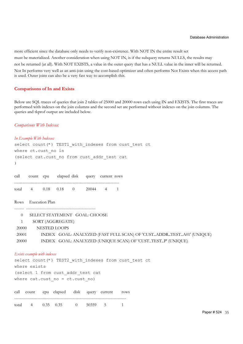
Below are SQL traces of queries that join 2 tables of 25000 and 20000 rows each using IN and EXISTS. The first traces are performed with indexes on the join columns and the second set are performed without indexes on the join columns. The queries and tkprof output are included below. Comparisons With Indexes: In Example With Indexes: select count(*) TEST1_with_indexes from cust_test ct where ct.cust_no in (select cat.cust_no from cust_addr_test cat )
call count cpu elapsed disk query current rows ----------------------------------------------------------------------------- total 4 0.18 0.18 0 20044 4 1 Rows Execution Plan ------- --------------------------------------------------- 0 SELECT STATEMENT GOAL: CHOOSE 1 SORT (AGGREGATE) 20000 NESTED LOOPS 20001 INDEX GOAL: ANALYZED (FAST FULL SCAN) OF 'CUST_ADDR_TEST_A01' (UNIQUE) 20000 INDEX GOAL: ANALYZED (UNIQUE SCAN) OF 'CUST_TEST_P' (UNIQUE) Exists example with indexes select count(*) TEST2_with_indexes from cust_test ct where exists (select 1 from cust_addr_test cat where cat.cust_no = ct.cust_no)
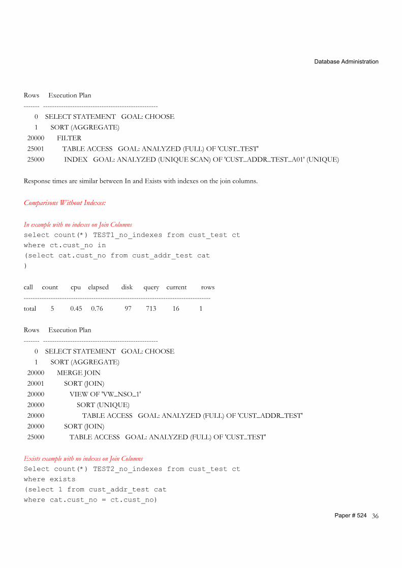
call count cpu elapsed disk query current rows ---------------------------------------------------------------------------------- total 4 0.35 0.35 0 50359 5 1
Database Administration
Paper # 524 36
Rows Execution Plan ------- --------------------------------------------------- 0 SELECT STATEMENT GOAL: CHOOSE 1 SORT (AGGREGATE) 20000 FILTER 25001 TABLE ACCESS GOAL: ANALYZED (FULL) OF 'CUST_TEST' 25000 INDEX GOAL: ANALYZED (UNIQUE SCAN) OF 'CUST_ADDR_TEST_A01' (UNIQUE) Response times are similar between In and Exists with indexes on the join columns. Comparisons Without Indexes: In example with no indexes on Join Columns select count(*) TEST1_no_indexes from cust_test ct where ct.cust_no in (select cat.cust_no from cust_addr_test cat )
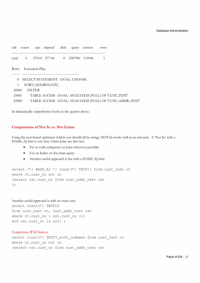
call count cpu elapsed disk query current rows ----------------------------------------------------------------------------------- total 5 0.45 0.76 97 713 16 1 Rows Execution Plan ------- --------------------------------------------------- 0 SELECT STATEMENT GOAL: CHOOSE 1 SORT (AGGREGATE) 20000 MERGE JOIN 20001 SORT (JOIN) 20000 VIEW OF 'VW_NSO_1' 20000 SORT (UNIQUE) 20000 TABLE ACCESS GOAL: ANALYZED (FULL) OF 'CUST_ADDR_TEST' 20000 SORT (JOIN) 25000 TABLE ACCESS GOAL: ANALYZED (FULL) OF 'CUST_TEST' Exists example with no indexes on Join Columns Select count(*) TEST2_no_indexes from cust_test ct where exists (select 1 from cust_addr_test cat where cat.cust_no = ct.cust_no)
Database Administration
Paper # 524 37
call count cpu elapsed disk query current rows ----------------------------------------------------------------------------------- total 4 270.01 277.04 0 5287981 115946 1 Rows Execution Plan ------- --------------------------------------------------- 0 SELECT STATEMENT GOAL: CHOOSE 1 SORT (AGGREGATE) 20000 FILTER 25001 TABLE ACCESS GOAL: ANALYZED (FULL) OF 'CUST_TEST' 25000 TABLE ACCESS GOAL: ANALYZED (FULL) OF 'CUST_ADDR_TEST' In dramatically outperforms Exists in the queries above. Comparisons of Not In vs. Not Exists Using the cost-based optimizer (which you should all be using), NOT In works well as an anti-join. A ‘Not In’ with a HASH_AJ hint is very fast. Outer Joins are also fast.
• Try to code subqueries as Joins wherever possible.
• Use an Index on the inner query
• Another useful approach is the with a HASH_AJ hint: select /*+ HASH_AJ */ count(*) TEST11 from cust_test ct where ct.cust_no not in (select cat.cust_no from cust_addr_test cat );
Another useful approach is with an outer join: select count(*) TEST12 from cust_test ct, cust_addr_test cat where ct.cust_no = cat.cust_no (+) and cat.cust_no is null ;
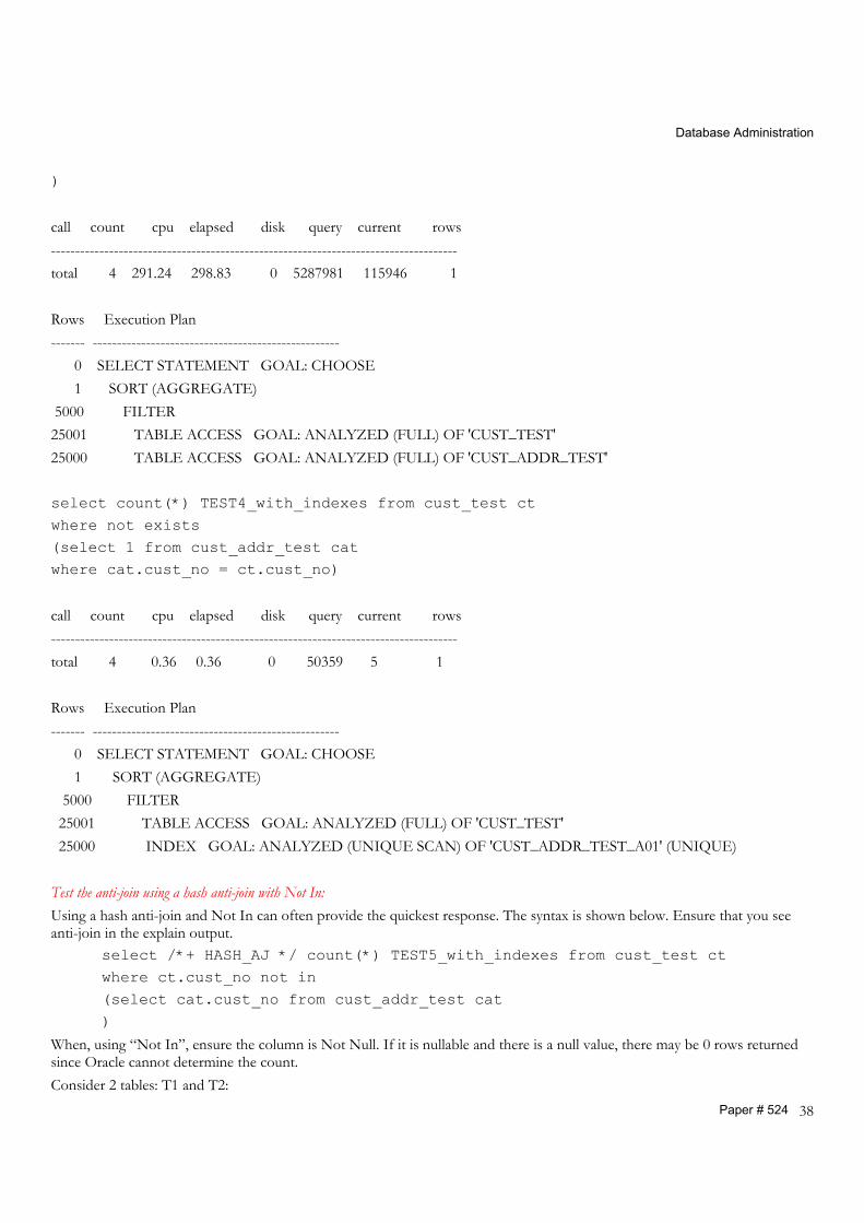
Comparisons With Indexes: select count(*) TEST3_with_indexes from cust_test ct where ct.cust_no not in (select cat.cust_no from cust_addr_test cat
Database Administration
Paper # 524 38
)
call count cpu elapsed disk query current rows ------------------------------------------------------------------------------------ total 4 291.24 298.83 0 5287981 115946 1 Rows Execution Plan ------- --------------------------------------------------- 0 SELECT STATEMENT GOAL: CHOOSE 1 SORT (AGGREGATE) 5000 FILTER 25001 TABLE ACCESS GOAL: ANALYZED (FULL) OF 'CUST_TEST' 25000 TABLE ACCESS GOAL: ANALYZED (FULL) OF 'CUST_ADDR_TEST' select count(*) TEST4_with_indexes from cust_test ct where not exists (select 1 from cust_addr_test cat where cat.cust_no = ct.cust_no)
call count cpu elapsed disk query current rows ------------------------------------------------------------------------------------ total 4 0.36 0.36 0 50359 5 1 Rows Execution Plan ------- --------------------------------------------------- 0 SELECT STATEMENT GOAL: CHOOSE 1 SORT (AGGREGATE) 5000 FILTER 25001 TABLE ACCESS GOAL: ANALYZED (FULL) OF 'CUST_TEST' 25000 INDEX GOAL: ANALYZED (UNIQUE SCAN) OF 'CUST_ADDR_TEST_A01' (UNIQUE) Test the anti-join using a hash anti-join with Not In: Using a hash anti-join and Not In can often provide the quickest response. The syntax is shown below. Ensure that you see anti-join in the explain output.
select /*+ HASH_AJ */ count(*) TEST5_with_indexes from cust_test ct where ct.cust_no not in (select cat.cust_no from cust_addr_test cat )
When, using “Not In”, ensure the column is Not Null. If it is nullable and there is a null value, there may be 0 rows returned since Oracle cannot determine the count. Consider 2 tables: T1 and T2:
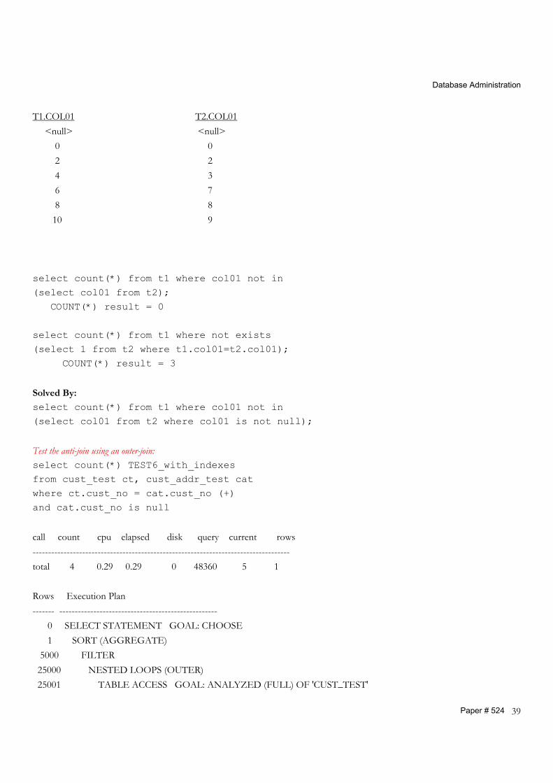
Database Administration
Paper # 524 39
T1.COL01 T2.COL01 <null> <null> 0 0 2 2 4 3 6 7 8 8 10 9 select count(*) from t1 where col01 not in (select col01 from t2); COUNT(*) result = 0 select count(*) from t1 where not exists (select 1 from t2 where t1.col01=t2.col01); COUNT(*) result = 3
Solved By:
select count(*) from t1 where col01 not in (select col01 from t2 where col01 is not null);
Test the anti-join using an outer-join: select count(*) TEST6_with_indexes from cust_test ct, cust_addr_test cat where ct.cust_no = cat.cust_no (+) and cat.cust_no is null
call count cpu elapsed disk query current rows ----------------------------------------------------------------------------------- total 4 0.29 0.29 0 48360 5 1 Rows Execution Plan ------- --------------------------------------------------- 0 SELECT STATEMENT GOAL: CHOOSE 1 SORT (AGGREGATE) 5000 FILTER 25000 NESTED LOOPS (OUTER) 25001 TABLE ACCESS GOAL: ANALYZED (FULL) OF 'CUST_TEST'
Database Administration
Paper # 524 40
20000 INDEX GOAL: ANALYZED (UNIQUE SCAN) OF 'CUST_ADDR_TEST_A01' (UNIQUE) The anti-joins above with using an outer join is very efficient.. USING MINUS
Some Databases use the MINUS operator to return rows from 1 table that do not exist in another. This can also achieve good performance. An example of an SQL statement using MINUS is shown below: Select customer_id, customer_name
from Customer
MINUS
Select customer_id, customer_name
from Invoice;
The above statement will show all Customers that have not been invoiced. Notice that when using MINUS, the number of columns and column types must be the same for the 2 queries. In this way, it is similar to the way that a Union statement operates. It is also limiting since all of the same columns and values used in the statements must exist in both tables - therefore there are many cases where the MINUS operator will not be useful.
Conclusion
• Become familiar with Oracle’s SQL functions. • Try out functions as well as your own solutions to problems. This can help you improve your SQL skills and can build
a repertoire that will help your most experienced developers.
• SQL is becoming more complicated.
• We can now do things in native SQL that used to only be possible in advanced query packages. o Get familiar with Oracle’s supplied PL/SQL packages
• Oracle is becoming more ansi SQL-92 and 99 compliant
• Also with 10g: SQL Model clause and regular expressions.
• SQL can be fun! (or at least interesting)