Embed Size (px)
Citation preview
87N.M. Adams and P.S. Freemont (eds.), Advances in Nuclear Architecture, DOI 10.1007/978-90-481-9899-3_3, © Springer Science+Business Media B.V. 2011
Abstract The spatial organisation of the genome in the cell nucleus has emerged as a key element to understand gene function. A wealth of molecular and microscopic information has been accumulated, resulting in a variety of – sometimes contradictory – models of nuclear architecture. So far, however, a large part of this structural infor-mation and in consequence also the models derived from them are ‘qualitative’. In this overview, a brief introduction will be given into quantitative experimental and modelling approaches to large scale nuclear genome architecture in human cells. As a biomedical application example, the use of a quantitative computer model of the 3D architecture allowed to explore different implications of nuclear structure on chromosomal aberrations. In addition, we shall present two novel examples for quantitative computer modelling: (1) The impact of SC 35 splicing domains on nuclear genome structure; (2) The dynamics of large scale nuclear genome struc-ture in a Brownian motion model. Finally, we shall discuss some perspectives to extend quantitative nuclear structure analysis to the nanoscale.
Keywords Nuclear architecture • Computer modelling • Chromatin domains • Dynamics • SC35 domains • Speckles • R-bands • Superresolution • lightoptical nanoscopy
D. Hübschmann and G. Kreth (*) Applied Optics and Information Processing, University Heidelberg, Im Neuenheimer Feld, D-69120, Heidelberg, Germany e-mail: [email protected]
N. Kepper Applied Optics and Information Processing and BioQuant Center, University Heidelberg, Im Neuenheimer Feld, D-69120, Heidelberg, Germany
C. Cremer (*) Applied Optics and Information Processing; BioQuant Center, Institute for Pharmacy and Molecular Biotechnology, University Heidelberg, Im Neuenheimer Feld, D-69120, Heidelberg, Germany and Institute for Molecular Biophysics, The Jackson laboratory, 04609 Bar Harbor, ME, USA e-mail: [email protected]
Chapter 3Quantitative Approaches to Nuclear Architecture Analysis and Modelling
Daniel Hübschmann, Nikolaus Kepper, Christoph Cremer, and Gregor Kreth
88 D. Hübschmann et al.
3.1 Introduction
A cell nucleus contains a hierarchy of connected levels of dynamical order: The first level is formed by the linear sequence of the of the nuclear DNA chains, in human cells about 2 × 3 109 base pairs. The second level is given by direct interactions between specific parts of the DNA chains and other macromolecules in the cell nucleus (Rippe et al. 2008). Specific proteins or protein complexes may bind to specific DNA sites and thus activate or silence specific genes. The third level of nuclear organization is the dynamic three dimensional organization of the DNA chains: For example, in each human lymphocyte, the about 2 m long DNA has to be packaged in such a way that it fits into the nucleus with a typical diameter of only 10 mm, and that nonetheless its information remains reliably accessible if required; information not required for a long time or the entire life of a specific cell has to be silenced in an effective way (Kepper et al. 2008). For example, genes required to be active during a given stage of development may have disastrous consequences if activated out of place. How are the profound differences in gene activities estab-lished and maintained in a large number of cell types to ensure the development and functioning of a complex multicellular organism (Cremer 1985; Cremer et al. 1988; Zuckerkandl 1997). To answer this question fully, in addition to nuclear biochemistry we need to understand how genomes are organized in the nuclei.
According to the role of a specific cell in the organism, different genes have to be activated and inactivated (“silenced”) in a very precise way, from the “totipotent” fertilized oocyte to “pluripotent” embryonic stem, cells to adult stem cells, to “termi-nally differentiated” cells. An understanding of how the activation and silencing of specific genes occur would greatly facilitate e.g., the reprogramming of adult stem cells (i.e. cells found in the body of an adult organism). Towards this goal, a large amount of highly relevant molecular and structural information has been accumulated. Many valuable attempts have been made to integrate this wealth of knowledge into models of nuclear architecture. Presently, however, most models of this kind are ‘qualitative’; this means that they describe certain general features of nuclear organisa-tion, without trying to quantitate them. By necessity, also the conclusions drawn from such models are qualitative. For example, for a long time it has been noted that the concept of ‘chromosome territories’ and their spatial distribution in the cell nucleus is a key element to understand the formation of chromosome aberrations. Nevertheless, such ideas by themselves did not allow to make quantitative predictions about the formation of cancer related chromosome aberrations in a given cell type at a given dose of ionizing radiation. Such a lack of prediction is not restricted to radiation effects but to many other biologically and medically important features of functional nuclear architecture.
The general idea of cellular biophysics is to overcome this impasse (a) by gaining as much quantitative information about relevant features as possible; (b) by using such quantitative information to develop ‘qualitative’ models into quantitative ones, i.e. into models which allow quantitative, observable predictions of certain param-eters; (c) by modifying the models in such a way that their predictive power is optimized. To be successful, this may require extensive efforts to develop the methods
893 Quantitative Approaches to Nuclear Architecture Analysis and Modelling
required to obtain the quantitative experimental information necessary for the predictive model calculations.
Concerning nuclear architecture and its biological and medical implications, until recently such a project was practically impossible to realize: On the experi-mental side, molecular information was missing; optical and labelling tools to perform quantitative analyses of nuclear structure on the level required were scarcely available; the computer hardware and the programmes to handle the huge amount of calculations were not existing.
In the following, some approaches to start such a programme towards quantitative nuclear architecture and modelling will be presented, based on the specific experi-ence of the authors.
3.2 Experimental Evidence for Nuclear Genome Large Scale Architecture
Numerous studies have shown that the chromatin fibers of individual chromosomes in the cell nucleus are not distributed throughout the nucleus but there enveloping surface forms a volume which occupies only a relatively small part of the nucleus.
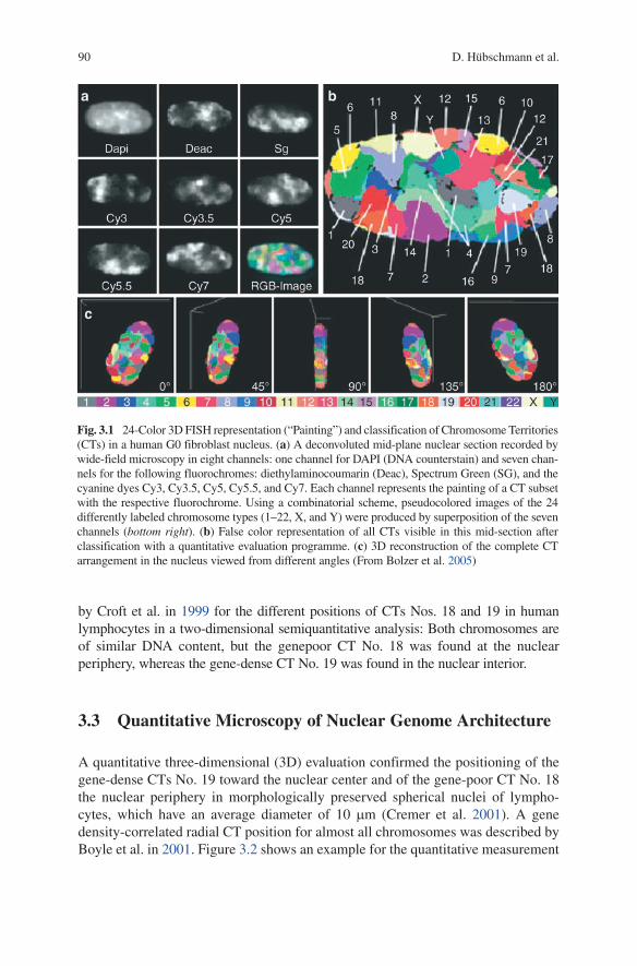
Figure 3.1 shows an example where all 24 chromosome types of the human genome were visualized by combinatorial Fluorescence-in situ Hybridization (FISH) (compare also Schroeck et al. 1996; Speicher et al. 1996).
The compartmentalization of the nucleus in several welldefined subregions such as nucleoli, nuclear bodies, chromosome territories (CTs), and their higher com-partmentalization levels into subchromosomal domains as well as the spatial arrangements of these compartments may have a profound impact on functional processes inside the nucleus (for review, see Chevret et al. 2000; Dundr and Misteli 2001; Cremer and Cremer 2001; Parada and Misteli 2002; O’Brien et al. 2003; Kreth et al. 2004a; Cremer et al. 2000; Cremer et al. 2006; Cremer and Cremer 2006a,b; Dietzel et al. 1998; Albiez et al. 2006; Ferreira et al. 1997; Zirbel et al. 1993; Cremer et al. 1993; Visser et al. 2000; Solovei et al. 2002; Qumsiyeh 1999; leitch 2000; Bridger 1999; Gonzalez-Melendi et al. 2000). For example, it has been shown that chromosome territories are compartmentalized into domains of early and later replicating chromatin (Visser et al. 1998; Zink et al. 1999; see also Tsukamoto et al. 2000): early replicating chromatin domains are found throughout the nucleus except for the utmost nuclear periphery and the perinucleolar space, whereas midreplicating chromatin domains form typical rims both along the nuclear periphery and around the nucleoli (Dimitrova and Berezney 2002). This specific arrangement of differently replicating chromatin may mirror the results of recent investigations, regarding the positioning of whole CTs inside the nuclear volume.
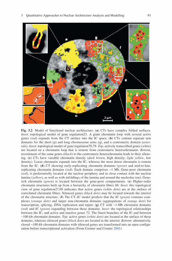
Figure 3.2 shows a ‘qualitative’ model of basic features nuclear architecture.Chromosome painting experiments of single CTs and groups of CTs in different
species suggest a relationship between the gene density of a chromosome and its radial positioning (distance to the nuclear center) in the nuclear volume. This was first shown
90 D. Hübschmann et al.
by Croft et al. in 1999 for the different positions of CTs Nos. 18 and 19 in human lymphocytes in a two-dimensional semiquantitative analysis: Both chromosomes are of similar DNA content, but the genepoor CT No. 18 was found at the nuclear periphery, whereas the gene-dense CT No. 19 was found in the nuclear interior.
3.3 Quantitative Microscopy of Nuclear Genome Architecture
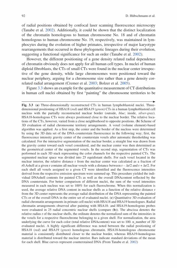
A quantitative three-dimensional (3D) evaluation confirmed the positioning of the gene-dense CTs No. 19 toward the nuclear center and of the gene-poor CT No. 18 the nuclear periphery in morphologically preserved spherical nuclei of lympho-cytes, which have an average diameter of 10 mm (Cremer et al. 2001). A gene density-correlated radial CT position for almost all chromosomes was described by Boyle et al. in 2001. Figure 3.2 shows an example for the quantitative measurement
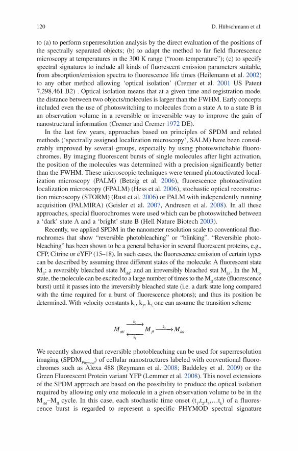
Fig. 3.1 24-Color 3D FISH representation (“Painting”) and classification of Chromosome Territories (CTs) in a human G0 fibroblast nucleus. (a) A deconvoluted mid-plane nuclear section recorded by wide-field microscopy in eight channels: one channel for DAPI (DNA counterstain) and seven chan-nels for the following fluorochromes: diethylaminocoumarin (Deac), Spectrum Green (SG), and the cyanine dyes Cy3, Cy3.5, Cy5, Cy5.5, and Cy7. Each channel represents the painting of a CT subset with the respective fluorochrome. Using a combinatorial scheme, pseudocolored images of the 24 differently labeled chromosome types (1–22, X, and Y) were produced by superposition of the seven channels (bottom right). (b) False color representation of all CTs visible in this mid-section after classification with a quantitative evaluation programme. (c) 3D reconstruction of the complete CT arrangement in the nucleus viewed from different angles (From Bolzer et al. 2005)
913 Quantitative Approaches to Nuclear Architecture Analysis and Modelling
Fig. 3.2 Model of functional nuclear architecture. (a) CTs have complex folded surfaces. Inset: topological model of gene regulation23. A giant chromatin loop with several active genes (red) expands from the CT surface into the IC space. (b) CTs contain separate arm domains for the short (p) and long chromosome arms (q), and a centromeric domain (aster-isks). Inset: topological model of gene regulation78,79. Top, actively transcribed genes (white) are located on a chromatin loop that is remote from centromeric heterochromatin. Bottom, recruitment of the same genes (black) to the centromeric heterochromatin leads to their silenc-ing. (c) CTs have variable chromatin density (dark brown, high density; light yellow, low density). loose chromatin expands into the IC, whereas the most dense chromatin is remote from the IC. (d) CT showing early-replicating chromatin domains (green) and mid-to-late-replicating chromatin domains (red). Each domain comprises ~1 Mb. Gene-poor chromatin (red), is preferentially located at the nuclear periphery and in close contact with the nuclear lamina (yellow), as well as with infoldings of the lamina and around the nucleolus (nu). Gene-rich chromatin (green) is located between the gene-poor compartments. (e) Higher-order chromatin structures built up from a hierarchy of chromatin fibres 88. Inset: this topological view of gene regulation27,68 indicates that active genes (white dots) are at the surface of convoluted chromatin fibres. Silenced genes (black dots) may be located towards the interior of the chromatin structure. (f) The CT–IC model predicts that the IC (green) contains com-plexes (orange dots) and larger non-chromatin domains (aggregations of orange dots) for transcription, splicing, DNA replication and repair. (g) CT with ~1-Mb chromatin domains (red) and IC (green) expanding between these domains. Inset: the topological relationships between the IC, and active and inactive genes 72. The finest branches of the IC end between ~100-kb chromatin domains. Top: active genes (white dots) are located at the surface of these domains, whereas silenced genes (black dots) are located in the interior. Bottom: alternatively, closed ~100-kb chromatin domains with silenced genes are transformed into an open configu-ration before transcriptional activation (From Cremer and Cremer 2001)
92 D. Hübschmann et al.
of radial positions obtained by confocal laser scanning fluorescence microscopy (Tanabe et al. 2002). Additionally, it could be shown that the distinct localization of the chromatin homologous to human chromosome No. 18 and of chromatin homologous to human chromosome No. 19, respectively, was maintained in lym-phocytes during the evolution of higher primates, irrespective of major karyotype rearrangements that occurred in these phylogenetic lineages during their evolution, suggesting a functional significance for such an order (Tanabe et al. 2002).
However, the different positioning of a gene density related radial dependence of chromatin obviously does not apply for all human cell types. In nuclei of human diploid fibroblasts, the CTs of small CTs were found in the nuclear center irrespec-tive of the gene density, while large chromosomes were positioned toward the nuclear periphery, arguing for a chromosome size rather than a gene density cor-related radial arrangement (Cremer et al. 2003; Bolzer et al. 2005).
Figure 3.3 shows an example for the quantitative measurement of CT distributions in human cell nuclei obtained by first “painting” the chromosome territories to be
Fig. 3.3 (a) Three-dimensionally reconstructed CTs in human lymphoblastoid nuclei. Three-dimensional positioning of HSA18 (red) and HSA19 (green) CTs in a human lymphoblastoid cell nucleus with the partially reconstructed nuclear border (outside, blue; inside, silver-gray). HSA18-homologous CTs were always positioned close to the nuclear border. The relative loca-tions of the CTs, however, varied from a close neighborhood to opposite positions. (b) Scheme of 3D evaluation of radial chromosome territory arrangements. A voxel (volume element)-based algorithm was applied. As a first step, the center and the border of the nucleus were determined by using the 3D data set of the DNA-counterstain fluorescence in the following way; first, the fluorescence intensity gravity center of the counterstain voxels after automatic thresholding was calculated. For the interactive segmentation of the nuclear border, a straight line was drawn from the gravity center toward each voxel considered, and the nuclear center was then determined as the geometrical center of the segmented voxels. In the second step, segmentation of CTs was performed in each 3D stack representing the color channels for the respective painted CTs. The segmented nuclear space was divided into 25 equidistant shells. For each voxel located in the nuclear interior, the relative distance r from the nuclear center was calculated as a fraction of r0.Ashell at a given r contains all nuclear voxels with a distance between r – Dr/2 and r + Dr/2. For each shell all voxels assigned to a given CT were identified and the fluorescence intensities derived from the respective emission spectrum were summed up. This procedure yielded the indi-vidual DNAshell contents for painted CTs as well as the overall DNAcontent reflected by the DNA counterstain. For better comparison of different nuclei, the sum of the voxel intensities measured in each nucleus was set to 100% for each fluorochrome. When this normalization is used, the average relative DNA content in nuclear shells as a function of the relative distance r from the 3D center represents the average radial distribution of the DNA representing the painted CTs or of the overall DNA in the entire set of evaluated nuclei. (c) Quantitative 3D evaluation of radial chromatin arrangements in primate cell nuclei with HSA18 and HSA19 homologues. Radial chromatin arrangements observed after painting with HSA18- and HSA19-homologous probes were evaluated in 25 radial concentric nuclear shells (compare (b)). The abscissa denotes the relative radius r of the nuclear shells, the ordinate denotes the normalized sum of the intensities in the voxels for a respective fluorochrome belonging to a given shell. For normalization, the area underlying the curve for each color (total relative DNAcontent) was set to 100. n_number of 3D evaluated nuclei. A highly significant difference was noted between the radial positioning of HSA18 (red) and HSA19 (green) homologous chromatin. HSA18-homologous chromosome material is consistently distributed closer to the nuclear border, whereas HSA19-homologous material is distributed toward the nuclear interior. Bars indicate standard deviations of the mean for each shell. Blue curves represent counterstained DNA (From Tanabe et al. 2002)

933 Quantitative Approaches to Nuclear Architecture Analysis and Modelling
nuclearshell
DNAcontent
chromosometerritory
0
r1
r0
0
100
r = r1r0
x 100
b
94 D. Hübschmann et al.
studied and then analyzing them by confocal laser scanning fluorescence microscopy (ClSM). Since their introduction, such quantitative measurements of chromatin distribution and other quantitative features have been amply used to convert qualita-tive information into quantitative ones. Only then, it became possible to compare nuclear structure with the quantitative predictions of computer models of nuclear architecture.
3.4 Quantitative Modeling of Nuclear Genome Large Scale Architecture
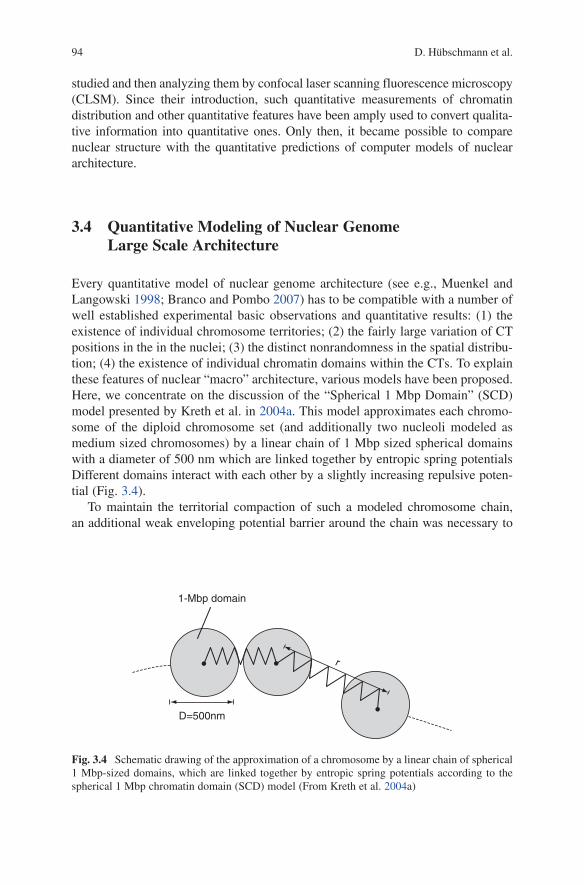
Every quantitative model of nuclear genome architecture (see e.g., Muenkel and langowski 1998; Branco and Pombo 2007) has to be compatible with a number of well established experimental basic observations and quantitative results: (1) the existence of individual chromosome territories; (2) the fairly large variation of CT positions in the in the nuclei; (3) the distinct nonrandomness in the spatial distribu-tion; (4) the existence of individual chromatin domains within the CTs. To explain these features of nuclear “macro” architecture, various models have been proposed. Here, we concentrate on the discussion of the “Spherical 1 Mbp Domain” (SCD) model presented by Kreth et al. in 2004a. This model approximates each chromo-some of the diploid chromosome set (and additionally two nucleoli modeled as medium sized chromosomes) by a linear chain of 1 Mbp sized spherical domains with a diameter of 500 nm which are linked together by entropic spring potentials Different domains interact with each other by a slightly increasing repulsive poten-tial (Fig. 3.4).
To maintain the territorial compaction of such a modeled chromosome chain, an additional weak enveloping potential barrier around the chain was necessary to
1-Mbp domain
D=500nm
r
Fig. 3.4 Schematic drawing of the approximation of a chromosome by a linear chain of spherical 1 Mbp-sized domains, which are linked together by entropic spring potentials according to the spherical 1 Mbp chromatin domain (SCD) model (From Kreth et al. 2004a)
953 Quantitative Approaches to Nuclear Architecture Analysis and Modelling
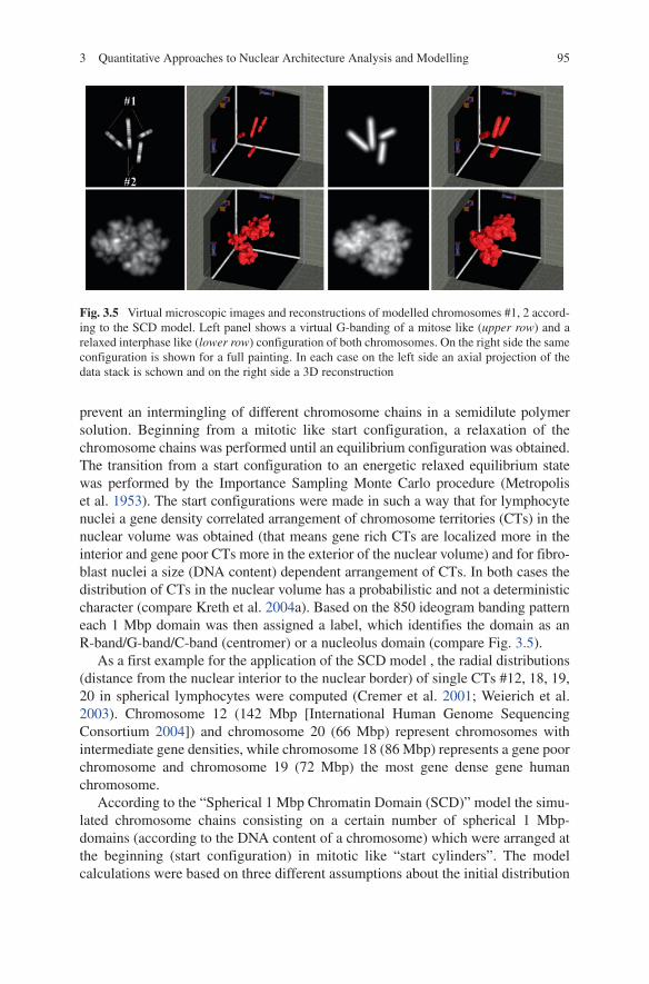
prevent an intermingling of different chromosome chains in a semidilute polymer solution. Beginning from a mitotic like start configuration, a relaxation of the chromosome chains was performed until an equilibrium configuration was obtained. The transition from a start configuration to an energetic relaxed equilibrium state was performed by the Importance Sampling Monte Carlo procedure (Metropolis et al. 1953). The start configurations were made in such a way that for lymphocyte nuclei a gene density correlated arrangement of chromosome territories (CTs) in the nuclear volume was obtained (that means gene rich CTs are localized more in the interior and gene poor CTs more in the exterior of the nuclear volume) and for fibro-blast nuclei a size (DNA content) dependent arrangement of CTs. In both cases the distribution of CTs in the nuclear volume has a probabilistic and not a deterministic character (compare Kreth et al. 2004a). Based on the 850 ideogram banding pattern each 1 Mbp domain was then assigned a label, which identifies the domain as an R-band/G-band/C-band (centromer) or a nucleolus domain (compare Fig. 3.5).
As a first example for the application of the SCD model , the radial distributions (distance from the nuclear interior to the nuclear border) of single CTs #12, 18, 19, 20 in spherical lymphocytes were computed (Cremer et al. 2001; Weierich et al. 2003). Chromosome 12 (142 Mbp [International Human Genome Sequencing Consortium 2004]) and chromosome 20 (66 Mbp) represent chromosomes with intermediate gene densities, while chromosome 18 (86 Mbp) represents a gene poor chromosome and chromosome 19 (72 Mbp) the most gene dense gene human chromosome.
According to the “Spherical 1 Mbp Chromatin Domain (SCD)” model the simu-lated chromosome chains consisting on a certain number of spherical 1 Mbp-domains (according to the DNA content of a chromosome) which were arranged at the beginning (start configuration) in mitotic like “start cylinders”. The model calculations were based on three different assumptions about the initial distribution
Fig. 3.5 Virtual microscopic images and reconstructions of modelled chromosomes #1, 2 accord-ing to the SCD model. left panel shows a virtual G-banding of a mitose like (upper row) and a relaxed interphase like (lower row) configuration of both chromosomes. On the right side the same configuration is shown for a full painting. In each case on the left side an axial projection of the data stack is schown and on the right side a 3D reconstruction
96 D. Hübschmann et al.
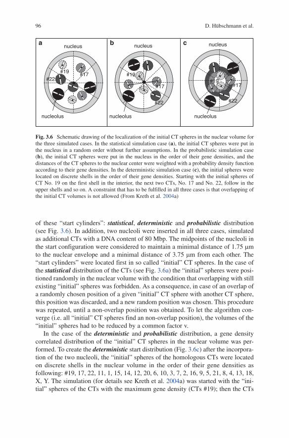
of these “start cylinders”: statistical, deterministic and probabilistic distribution (see Fig. 3.6). In addition, two nucleoli were inserted in all three cases, simulated as additional CTs with a DNA content of 80 Mbp. The midpoints of the nucleoli in the start configuration were considered to maintain a minimal distance of 1.75 mm to the nuclear envelope and a minimal distance of 3.75 mm from each other. The “start cylinders” were located first in so called “initial” CT spheres. In the case of the statistical distribution of the CTs (see Fig. 3.6a) the “initial” spheres were posi-tioned randomly in the nuclear volume with the condition that overlapping with still existing “initial” spheres was forbidden. As a consequence, in case of an overlap of a randomly chosen position of a given “initial” CT sphere with another CT sphere, this position was discarded, and a new random position was chosen. This procedure was repeated, until a non-overlap position was obtained. To let the algorithm con-verge (i.e. all “initial” CT spheres find an non-overlap position), the volumes of the “initial” spheres had to be reduced by a common factor v.
In the case of the deterministic and probabilistic distribution, a gene density correlated distribution of the “initial” CT spheres in the nuclear volume was per-formed. To create the deterministic start distribution (Fig. 3.6c) after the incorpora-tion of the two nucleoli, the “initial” spheres of the homologous CTs were located on discrete shells in the nuclear volume in the order of their gene densities as following: #19, 17, 22, 11, 1, 15, 14, 12, 20, 6, 10, 3, 7, 2, 16, 9, 5, 21, 8, 4, 13, 18, X, Y. The simulation (for details see Kreth et al. 2004a) was started with the “ini-tial” spheres of the CTs with the maximum gene density (CTs #19); then the CTs
nucleus
nucleolus
#22#19 #17
nucleus
#22
#19
#17
nucleolus
a b c nucleus
#22
nucleolus
#19#17
Fig. 3.6 Schematic drawing of the localization of the initial CT spheres in the nuclear volume for the three simulated cases. In the statistical simulation case (a), the initial CT spheres were put in the nucleus in a random order without further assumptions. In the probabilistic simulation case (b), the initial CT spheres were put in the nucleus in the order of their gene densities, and the distances of the CT spheres to the nuclear center were weighted with a probability density function according to their gene densities. In the deterministic simulation case (c), the initial spheres were located on discrete shells in the order of their gene densities. Starting with the initial spheres of CT No. 19 on the first shell in the interior, the next two CTs, No. 17 and No. 22, follow in the upper shells and so on. A constraint that has to be fulfilled in all three cases is that overlapping of the initial CT volumes is not allowed (From Kreth et al. 2004a)
973 Quantitative Approaches to Nuclear Architecture Analysis and Modelling
#17 spheres with the second highest gene density were located with an appropriate distance from the first shell and so on. In this deterministic start distribution, all probabilistic constraints were eliminated, except that on a given shell surface, an “initial” CT sphere was allowed any radial position not resulting in an overlap.
For the probabilistic case (Fig. 3.6b), after the incorporation of the two nucleoli, the CTs were put into the nuclear volume in the same order according to gene den-sity as realized for the deterministic case. Here, however, in contrast to the deter-ministic case, the “initial” CT spheres were not located on discrete shells but the distance from the center of the “initial” spheres to the nuclear center was weighted with an exponential probability density function which depends on the gene density of a given chromosome. A non overlapping position of the CT in the nucleus was chosen. Then the distance d to the nuclear center was determined for this special position, and a probability vaule P(d) was calculated with the gene density of CT A (e.g., #22). Then the calculated P(d) value was compared with a random number between 0 and 1. If the random number turned out to be equal or larger than the calculated P(d) value, then the position of the “initial” (CT A) sphere was accepted. If the random number turned out to be smaller than the calculated P(d) value, then again a new randomly chosen position for CT A was tested for non overlap; the d value of the new non overlapping position was again inserted in Eq. (3.8) and tested as described above. The procedure was continued until a non-overlap position was obtained with a random number equal/larger than the P(d).
For the gene density values applied for each CT, sequence data derived ratios were used of observed versus expected gene-based ETS markers per chromosome (Deloukas et al. 1998).
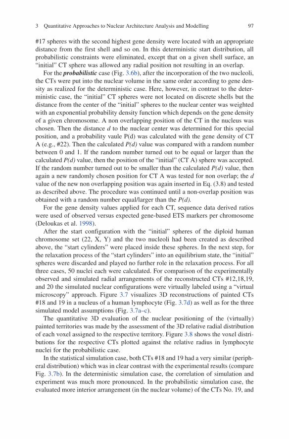
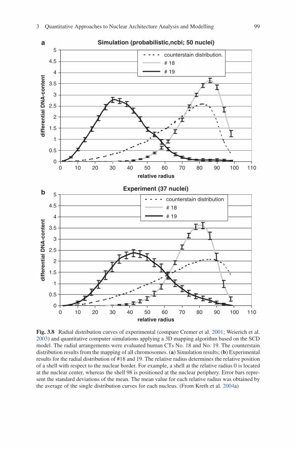
After the start configuration with the “initial” spheres of the diploid human chromosome set (22, X, Y) and the two nucleoli had been created as described above, the “start cylinders” were placed inside these spheres. In the next step, for the relaxation process of the “start cylinders” into an equilibrium state, the “initial” spheres were discarded and played no further role in the relaxation process. For all three cases, 50 nuclei each were calculated. For comparison of the experimentally observed and simulated radial arrangements of the reconstructed CTs #12,18,19, and 20 the simulated nuclear configurations were virtually labeled using a “virtual microscopy” approach. Figure 3.7 visualizes 3D reconstructions of painted CTs #18 and 19 in a nucleus of a human lymphocyte (Fig. 3.7d) as well as for the three simulated model assumptions (Fig. 3.7a–c).
The quantitative 3D evaluation of the nuclear positioning of the (virtually) painted territories was made by the assessment of the 3D relative radial distribution of each voxel assigned to the respective territory. Figure 3.8 shows the voxel distri-butions for the respective CTs plotted against the relative radius in lymphocyte nuclei for the probabilistic case.
In the statistical simulation case, both CTs #18 and 19 had a very similar (periph-eral distribution) which was in clear contrast with the experimental results (compare Fig. 3.7b). In the deterministic simulation case, the correlation of simulation and experiment was much more pronounced. In the probabilistic simulation case, the evaluated more interior arrangement (in the nuclear volume) of the CTs No. 19, and
98 D. Hübschmann et al.
the more peripheral arrangement of the CTs No. 18, fitted the experimental data best. These examples (Kreth et al. 2004a) indicate that already relatively basic quantitative models allow to predict nuclear genome macrostructure (here the radial distribution of specific CTs) in a promising way.
3.5 Application of the SCD Computer Model to Predict Cell Type Specific Radiation-Induced Chromosomal Aberrations
The non random higher order spatial arrangement of chromosome territories (CTs) and specific genomic regions in eukaryotic cells significantly contributes to their likelihood of undergoing chromosomal aberrations once chromosome breaks have occurred (Kozubek et al. 1999; Cornforth et al. 2002; Roix et al. 2003; Arsuaga et al. 2004;
Fig. 3.7 Visualization of reconstructed CTs of simulated human cell nuclei (a–c) according to the SCD model and of an experimental human lymphocyte cell nucleus with FISH-painted CTs. (d) The simulated virtual microscopy data stacks are reconstructions from the three simulation cases of the relaxed configurations: statistical simulation case (a), probabilistic simulation case (b), and deterministic simulation case (c). In all cases, CTs No. 18 were visualized in red and CTs No. 19 in green. The visualization tool was kindly provided by Dr. R. Heintzmann, University Jena,Germany (From Kreth et al. 2004a)
993 Quantitative Approaches to Nuclear Architecture Analysis and Modelling
Simulation (probabilistic,ncbi; 50 nuclei)a
b
0
0.5
1
1.5
2
2.5
3
3.5
4
4.5
5
0 10 20 30 40 50 60 70 80 90 100 110
relative radius
0 10 20 30 40 50 60 70 80 90 100 110relative radius
dif
fere
nti
al D
NA
-co
nte
nt
0
0.5
1
1.5
2
2.5
3
3.5
4
4.5
5
dif
fere
nti
al D
NA
-co
nte
nt
counterstain distribution.
# 18
# 19
Experiment (37 nuclei)
counterstain distribution
# 18
# 19
Fig. 3.8 Radial distribution curves of experimental (compare Cremer et al. 2001; Weierich et al. 2003) and quantitative computer simulations applying a 3D mapping algorithm based on the SCD model. The radial arrangements were evaluated human CTs No. 18 and No. 19. The counterstain distribution results from the mapping of all chromosomes. (a) Simulation results; (b) Experimental results for the radial distribution of #18 and 19. The relative radius determines the relative position of a shell with respect to the nuclear border. For example, a shell at the relative radius 0 is located at the nuclear center, whereas the shell 98 is positioned at the nuclear periphery. Error bars repre-sent the standard deviations of the mean. The mean value for each relative radius was obtained by the average of the single distribution curves for each nucleus. (From Kreth et al. 2004a)
100 D. Hübschmann et al.
Parada et al. 2004). In lymphocytes, CTs are arranged in a radial manner which is evolutionarily conserved in lymphocytes (Tanabe et al. 2002) and has also been reported in fibroblasts. However, while in lymphocyte type cell nuclei the gene density seems to be the underlying factor arranging gene dense chromosomes in the interior and gene poor chromosomes in the periphery of the nuclear volume (e.g., Boyle et al. 2001; Cremer et al. 2001) , in fibroblast nuclei a high correlation with the size was reported (Sun et al. 2000; Bolzer et al. 2005). Radial positioning is also not limited to entire chromosomes, but has also been reported for single genes (Roix et al. 2003). For all these experimentally observed radial patterns, the probabilistic nature is a common further feature. That means, although average positions of genes and chromosomes, relative to the center of the nucleus or relative to each other, can be measured in absolute terms, the position of a single gene region or chromosome varies greatly among cells in a population.
To evaluate specific aspects of radiation induced aberrations, quantitative models based on nuclear architecture have been applied (Sachs et al. 1997; Sachs et al. 2000; Arsuaga et al. 2004). In these models regard, a geometric representation of the chromosomes in a given nuclear volume was used (Holley et al. 2002; Friedland et al. 2008;. Ballarini et al. 2002). For example, to attend on the lower order chro-matin level break point formations, Holley et al. (2002) described the CT structure by a polymer, in which the 30 nm fiber was allowed to form a three-dimensional random walk within a spherical chromosome volume. To construct irregularly shaped CT volumes, Ballarini et al. (2002) presented a model where the nuclear volume was first divided in a 3D grid of 27,000 cubic elements (boxes) and CTs were constructed then by subsequent occupation of closest neighboring boxes. In both model approaches the volumes of CTs were proportional to their DNA con-tents; a specific arrangement of gene dense or gene poor chromosomes in the nuclear volume or a size dependent arrangement however was not regarded.
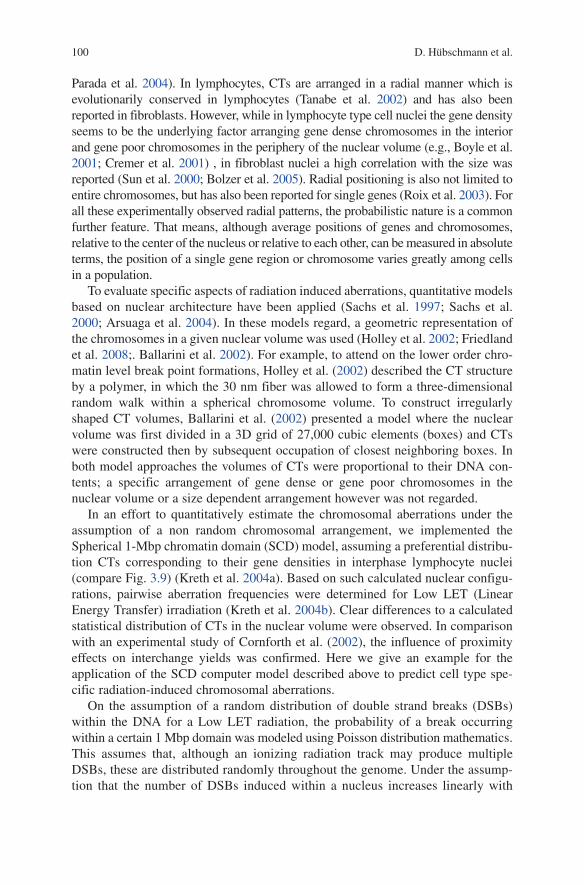
In an effort to quantitatively estimate the chromosomal aberrations under the assumption of a non random chromosomal arrangement, we implemented the Spherical 1-Mbp chromatin domain (SCD) model, assuming a preferential distribu-tion CTs corresponding to their gene densities in interphase lymphocyte nuclei (compare Fig. 3.9) (Kreth et al. 2004a). Based on such calculated nuclear configu-rations, pairwise aberration frequencies were determined for low lET (linear Energy Transfer) irradiation (Kreth et al. 2004b). Clear differences to a calculated statistical distribution of CTs in the nuclear volume were observed. In comparison with an experimental study of Cornforth et al. (2002), the influence of proximity effects on interchange yields was confirmed. Here we give an example for the application of the SCD computer model described above to predict cell type spe-cific radiation-induced chromosomal aberrations.
On the assumption of a random distribution of double strand breaks (DSBs) within the DNA for a low lET radiation, the probability of a break occurring within a certain 1 Mbp domain was modeled using Poisson distribution mathematics. This assumes that, although an ionizing radiation track may produce multiple DSBs, these are distributed randomly throughout the genome. Under the assump-tion that the number of DSBs induced within a nucleus increases linearly with
1013 Quantitative Approaches to Nuclear Architecture Analysis and Modelling
dose and is proportional to the DNA content of the cell, the probability pn of an
individual modeled 1 Mbp domain containing n DSBs was calculated from an adaptation of the equation of Poisson distribution (Johnston et al. 1997).
The DSBs within the 1 Mbp domains were placed randomly. To determine an exchange (inter-/intra-change) between two DSBs in two 1 Mbp domains, only those 1 Mbp domains containing DSBs were regarded which revealed a distance (the distance between the mid points of both 1 Mbp domains) smaller or equal to a certain proximity value. Besides the proximity value of 500 nm (Kreth et al. 2004b), also a proximity value of 250 nm (which means that the 1 Mbp domains must overlap) and also proximity values of 750 and 1,000 nm were tested. An exchange event in dependence of the distance d between the two DSBs in the two domains was counted according to the normalized probability function p
d = [r/d]a.
Here, r denotes the radius of a 1 Mbp domain which determines the maximal dis-tance by which an exchange takes place in every case. For the exponent a different values were tested and compared with experimentally obtained dose response curves (Fig. 3.10). When for a certain DSB an exchange was not counted, other domains in a certain distance (proximity value, see above) containing DSBs were tested. When this procedure failed, the DSB was considered as repaired. Exchanges between domains of the same chromosome were counted as intrachanges and were separated from interchanges (For details see Kreth et al. 2007).
These application examples show that the prediction of radiation induced chromo-some aberrations in human lymphycyte can be highly improved on the basis of com-puter models taking into regard quantitative structural information. With a reasonable parameter set, the Spherical 1 Mbp Chromatin Domain (SCD) model allowed an excellent agreement (with respect to the amount and the behavior) of calculated dicentrics/translocation frequencies with experimental dose response curves in a
Fig. 3.9 Visualization of a modeled lymphocyte nucleus according to the SCD model. (a) Visualization of the complete diploid chromosome set of the human genome after 400,000 Monte Carlo steps. Each homologous chromosome pair is labeled in a separate color. (b) The two gene poor CTs #18 and 21 are visualized only. The peripheral organization is clearly visible. (c) The three gene rich CTs #17, 19, 22 are visualized; here the internal positioning near the nuclear center is preferred according to the experimental observations. The bar denotes 5 mm (From Kreth et al. 2007)
Dose response curves (1 Mbp resolution)
Dose response curves (1 Mbp resolution)
Dose [Gy]
Rec
ipro
cal T
rans
loca
tions
or
Dic
entr
ics/
Cel
lR
ecip
roca
l Tra
nslo
catio
ns o
r D
icen
tric
s/C
ell
00
0.5
1
1.5
2
2.5
3
0
0.5
1
1.5
2
2.5
3
3.5
4
1 2 3 4 5
Dose [Gy]
a
b
0 1 2 3 4 5
different exponents of the distance function
different proximity values
SCD model, a=1.4SCD model, a=2
SCD model, a=3
SCD model, a=4SCD model, a=5
Dicentrics: X-Ray (Lloyd et al. 1986)
Dicentrics: Co-60 (Edwards et al. 1997)
SCD model, 1000nmSCD model, proximity: 750nm
SCD model, proximity: 500nm
SCD model, proximity: 250nm
Dicentrics: X-Ray (Lloyd et al. 1986)
Dicentrics: Co-60 (Edwards et al. 1997)
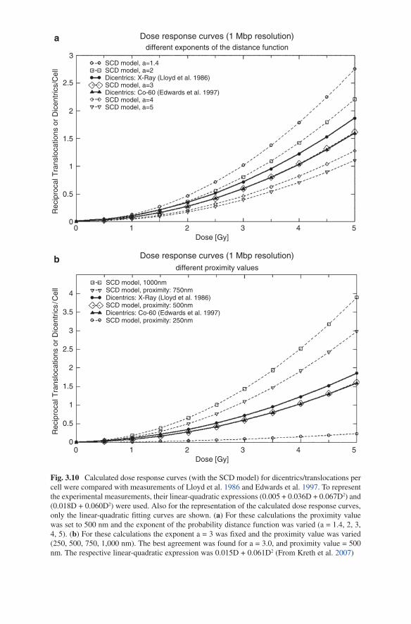
Fig. 3.10 Calculated dose response curves (with the SCD model) for dicentrics/translocations per cell were compared with measurements of lloyd et al. 1986 and Edwards et al. 1997. To represent the experimental measurements, their linear-quadratic expressions (0.005 + 0.036D + 0.067D2) and (0.018D + 0.060D2) were used. Also for the representation of the calculated dose response curves, only the linear-quadratic fitting curves are shown. (a) For these calculations the proximity value was set to 500 nm and the exponent of the probability distance function was varied (a = 1.4, 2, 3, 4, 5). (b) For these calculations the exponent a = 3 was fixed and the proximity value was varied (250, 500, 750, 1,000 nm). The best agreement was found for a = 3.0, and proximity value = 500 nm. The respective linear-quadratic expression was 0.015D + 0.061D2 (From Kreth et al. 2007)
1033 Quantitative Approaches to Nuclear Architecture Analysis and Modelling
range between 0.5–5 Gy. Calculating a high number of nuclear structure configura-tions (one million), it was possible to predict absolute interchange frequencies for radiation doses in the 2–5 Gy range.
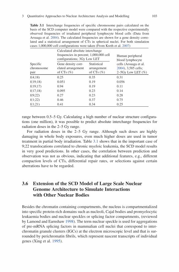
For radiation doses in the 2–5 Gy range. Although such doses are highly damaging in whole body exposures, even much higher doses are used in tumor treatment in partial body irradiation. Table 3.1 shows that in the important case of 9;22 translocations correlated to chronic myeloic leukemia, the SCD model results in very good predictions. In other cases, the correlation between prediction and observation was not as obvious, indicating that additional features, e.g., different compaction levels of CTs, differential repair rates, or selections against certain aberrations have to be regarded.
3.6 Extension of the SCD Model of Large Scale Nuclear Genome Architecture to Simulate Interactions with Other Nuclear Bodies
Besides the chromatin containing compartments, the nucleus is compartmentalized into specific protein-rich domains such as nucleoli, Cajal bodies and promyelocytic leukaemia bodies and nuclear speckles or splicing factor compartments, (reviewed by lamond and Earnshaw 1998). The term nuclear speckle is used for aggregations of pre-mRNA splicing factors in mammalian cell nuclei that correspond to inter-chromatin granule clusters (IGCs) at the electron microscopic level and that is sur-rounded by perichromatin fibrils, which represent nascent transcripts of individual genes (Xing et al. 1995).
Table 3.1 Interchange frequencies of specific chromosome pairs calculated on the basis of the SCD computer model were compared with the respective experimentally observed frequencies of irradiated peripheral lymphocyte blood cells (Data from Arsuaga et al. 2004). The calculated frequencies are shown for a gene density corre-lated and a statistical arrangement of CTs in spherical nuclei. For both simulation cases 1,000,000 cell configurations were taken (From Kreth et al. 2007)
Specific chromosome pair
Calculated absolute interchange frequencies in percent; 1,000,000 cell configurations; 3Gy low lET
Human peripheral blood lymphocyte cells (Arsuaga et al. 2004), 3,585 cells; 2–5Gy low lET (%)
Gene density corr-elated arrangement of CTs (%)
Statistical arrangement of CTs (%)
f(4;18) 0.25 0.35 0.31f(19;18) 0.051 0.19 0.056f(19;17) 0.94 0.19 0.11f(17;18) 0.095 0.23 0.14f(9;22) 0.27 0.23 0.28f(1;22) 0.46 0.37 0.75f(1;21) 0.41 0.34 0.25
104 D. Hübschmann et al.
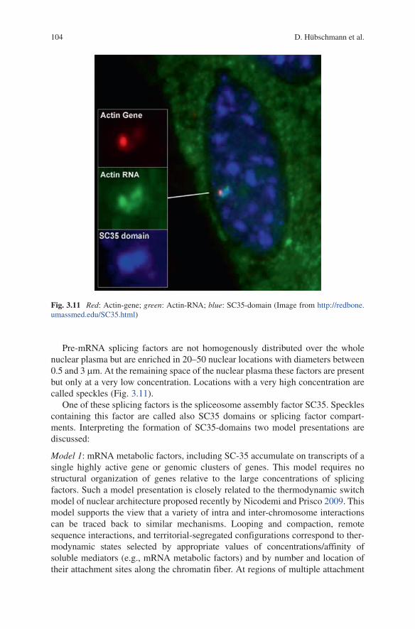
Pre-mRNA splicing factors are not homogenously distributed over the whole nuclear plasma but are enriched in 20–50 nuclear locations with diameters between 0.5 and 3 mm. At the remaining space of the nuclear plasma these factors are present but only at a very low concentration. locations with a very high concentration are called speckles (Fig. 3.11).
One of these splicing factors is the spliceosome assembly factor SC35. Speckles containing this factor are called also SC35 domains or splicing factor compart-ments. Interpreting the formation of SC35-domains two model presentations are discussed:
Model 1: mRNA metabolic factors, including SC-35 accumulate on transcripts of a single highly active gene or genomic clusters of genes. This model requires no structural organization of genes relative to the large concentrations of splicing factors. Such a model presentation is closely related to the thermodynamic switch model of nuclear architecture proposed recently by Nicodemi and Prisco 2009. This model supports the view that a variety of intra and inter-chromosome interactions can be traced back to similar mechanisms. looping and compaction, remote sequence interactions, and territorial-segregated configurations correspond to ther-modynamic states selected by appropriate values of concentrations/affinity of soluble mediators (e.g., mRNA metabolic factors) and by number and location of their attachment sites along the chromatin fiber. At regions of multiple attachment
Fig. 3.11 Red: Actin-gene; green: Actin-RNA; blue: SC35-domain (Image from http://redbone.umassmed.edu/SC35.html)
1053 Quantitative Approaches to Nuclear Architecture Analysis and Modelling
sites a larger number of factors will accumulated which might result then in aggre-gations of SC-35 domains.
Model 2: Multiple genes cluster at the periphery of a single large accumulation of mRNA metabolic factors. R-band DNA, which is gene rich, is more intimately associated with these SC-35 domains than gene poor G-band DNA. This view is experimentally supported by studies of FISH labelled R-bands, SC-35 domains and a subset of genes (Shopland et al. 2003). The studies revealed that each chromo-some territory associates with three or four SC-35 domains, indicating specialized regions at the chromosome territory periphery. These contain domain-associated genes that can even come from different chromosome arms. An SC-35 domain can also associate with genes from different chromosomes. Because domain choice for individual genes is often random, the relative positions of their respective chromo-somes also may be highly variable. The clustering of multiple specific genes and extensions of R-band DNA around the periphery of SC-35 domains reflects an organization around a structure, rather than of factors simply collected on the tran-scripts of a highly expressed gene.
To translate these experimental findings in a quantitative model representation in the present contribution the 1 Mbp Spherical Chromatin Domain (SCD) model was extended to regard attractive interactions of gene rich R-band domains with pre existing spherical SC35 domains according to Model 2. This approach (presented here for the first time)allows it for the first time to evaluate the influences from protein – chromatin interactions on the higher order nuclear architecture.
3.6.1 SCD model and banding pattern
To model the interaction between chromatin (the 1 Mbp SCD R/G band domains of chromosome territories), additional interactions between the introduced SC35-domains and the respective R-band/G-band domains were introduced. For the realization of combined attractive and repulsive interactions the lennard Jones
potential is commonly used. This potential consist on the attractive part 6
x
σ − and
the repulsive part 12
x
σ . The following interactions were implemented:
SC35-domain and R-band domain (attractive and repulsive):
12 6
1 11 1( ) 4 ·V x
x x
σ σ = ε −
SC35-domain and G-band domain (repulsive):
12 6
2 22 2 2 min,2
2 min,2
( ) 4 · if
( ) 0 if
V x x rx x
V x x r
σ σ = ε − + ε ≤ = >
106 D. Hübschmann et al.
SC35-domain and SC35-domain (repulsive):
12 6
3 33 3 3 min,3
3 min,3
( ) 4 · if
( ) 0 if
V x x rx x
V x x r
= ε − + ε ≤ = >
σ σ
The potential depth e describes the strength of the potential between the respective interacting domains at distance x, s the null position and r
min the minimum of the
potential.For the model calculation a mean number of 30 spherical SC35 domains with a
mean diameter of 1.5 mm were introduced. The values for the potential strength e2
between two speckles and for the potential strength e3 between G-band domains
and speckles were chosen to correspond to 1.5 kT which is identical with the inter-action potential strength e
0 between two 1 Mbp domains. This value ensured that a
complete penetration of different domains during the relaxation process was pre-vented (Fig. 3.12).
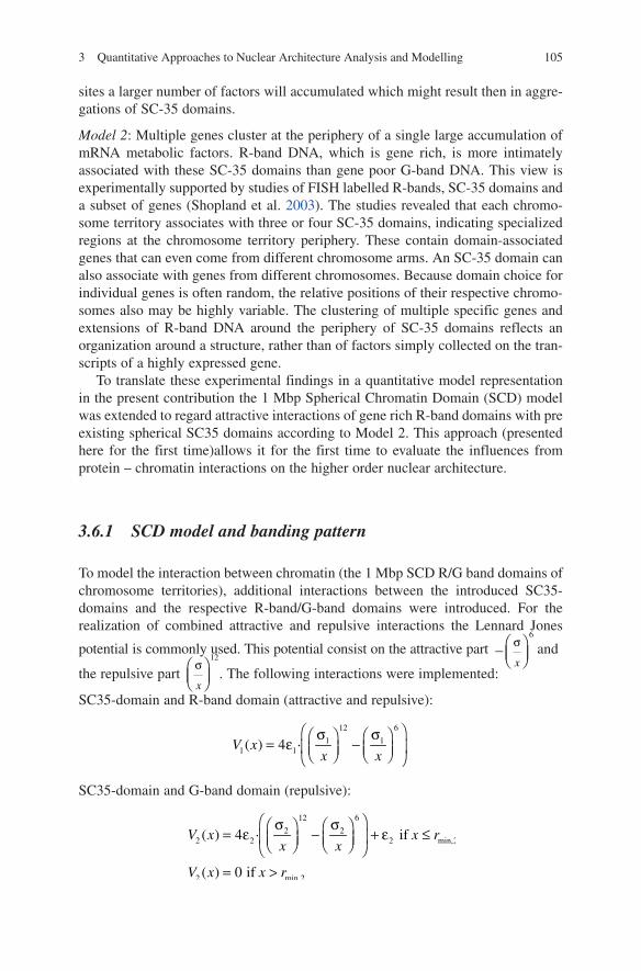
Fig. 3.12 Mitotic like start configuration (upper row) and relaxed interphase configurations (lower row) of a spherical shaped lymphocyte nucleus (left side; 10 mm in diameter) and an ellip-soidal shaped fibroblast nucleus (right side; 20 mm in diameter) together with 30 SC35 domains are shown (visualized in white). A SC35 domain has a diameter of 1.5 mm
1073 Quantitative Approaches to Nuclear Architecture Analysis and Modelling
3.6.2 Calibration
The value of the parameter e1 of the interaction potential between R-band domains
and SC 35 domains was varied between e1 = 0.0 and e
1 = 12.0 kT, where as for the
range e1 = 0.0–2.0 kT a smaller step width was chosen and for the range e
1=2.0–12.0 kT
a larger step width. For each chosen value of e1 an ensemble of four relaxations was
calculated. To obtain an optimal setting for e1 in the model which satisfy best the
experimental observations two criteria were chosen:Criteria I: all contacts between G-band domains with SC35 domains
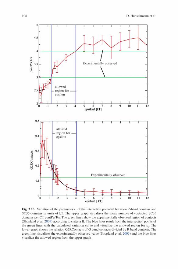
(Gbandcounts) and all contacts between R-band domains with SC35 domains (Rbandcounts) were summed up and the ratio G2RContacts was determined as the quotient between Gbandcounts and Rbandcounts. This ratio was experimentally observed by Shopland et al. (2003) to a value of 1/8.
Criteria II: The mean number of contacted SC35 domains per CT was saved in the variable contPerTer. Mean values for this variable between 3 and 4 were experimentally observed by Shopland et al. (2003).
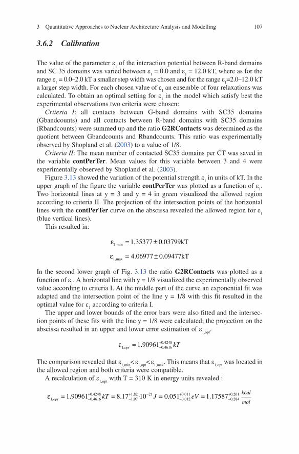
Figure 3.13 showed the variation of the potential strength e1 in units of kT. In the
upper graph of the figure the variable contPerTer was plotted as a function of e1.
Two horizontal lines at y = 3 and y = 4 in green visualized the allowed region according to criteria II. The projection of the intersection points of the horizontal lines with the contPerTer curve on the abscissa revealed the allowed region for e
1
(blue vertical lines).This resulted in:
1,min 1.35377 0.03799kT=ε ±
1,max 4.06977 0.09477kT=ε ±
In the second lower graph of Fig. 3.13 the ratio G2RContacts was plotted as a function of e
1. A horizontal line with y = 1/8 visualized the experimentally observed
value according to criteria I. At the middle part of the curve an exponential fit was adapted and the intersection point of the line y = 1/8 with this fit resulted in the optimal value for e
1 according to criteria I.
The upper and lower bounds of the error bars were also fitted and the intersec-tion points of these fits with the line y = 1/8 were calculated; the projection on the abscissa resulted in an upper and lower error estimation of e
1,opt.
0.42481, 0.46161.90961opt kT+
−=ε
The comparison revealed that e1,min
< e1,opt
< e1,max
. This means that e1,opt
was located in the allowed region and both criteria were compatible.
A recalculation of e1,opt
with T = 310 K in energy units revealed :
0.4248 1.82 21 0.011 0.2611, 0.4616 1.97 0.012 0.2841.90961 8.17 ·10 0.051 1.17587opt
kcal
molkT J eV+ + − + +
− − − −= = =ε =
108 D. Hübschmann et al.
Experimentally observed
cont
Per
Ter
G2R
Con
tact
s
Experimentally observed
allowedregion forepsilon
allowedregion forepsilon
Fig. 3.13 Variation of the parameter e1 of the interaction potential between R-band domains and
SC35-domains in units of kT. The upper graph visualizes the mean number of contacted SC35 domains per CT contPerTer. The green lines show the experimentally observed region of contacts (Shopland et al. 2003) according to criteria II. The blue lines result from the intersection points of the green lines with the calculated variation curve and visualize the allowed region for e
1. The
lower graph shows the relation G2RContacts of G band contacts divided by R band contacts. The green line visualizes the experimentally observed value (Shopland et al. 2003) and the blue lines visualize the allowed region from the upper graph
1093 Quantitative Approaches to Nuclear Architecture Analysis and Modelling
Hydrogen bonds in solution have a binding energy of:
~ 1H
kcal
molε
Comparing both values one can conclude in a very rough first estimation that the interaction strength between R-band domains and SC35 domains might be in the order of only 1.18 hydrogen bonds, despite of the quite large contact surface which would allow a much larger number.
In a second calculation the size of the SC35 domains was reduced from 1.5 to 1.0 mm. In this case the value e
1,opt was reduced slightly to e
1,opt = 1.56139 kT.
However it could be shown that this reduced size for a S35 domain is not longer compatible with the experimentally observed criteria I, II (calculations were not shown here).
3.6.3 Comparison with Experimental Observations
Taking into account the calculated optimal value 0.42481, 0.46161.90961opt kT+
−=ε an ensemble set of 204 relaxed configurations were simulated and the respective val-ues for criteria I,II were calculated (compare Table 3.2). In addition to the both criteria I, II the number of contacts of chromatin domains of two specific gene regions with the SC35 domains were also analyzed according to the experimental setup of Shopland et al. (2003).
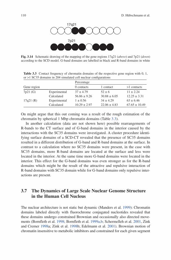
The gene region 17q21 consists on ten chromatin domains and corresponds to a major part to a R-band and the 7p21 gene region consists on nine chromatin domains and the major part of this region is a G-band (compare Fig. 3.14).
The comparison of the calculated contact frequencies with the SCD model and the experimentally observed frequencies (compare Table 3.3) revealed a very good agreement for more than one contacts (between domains of the respective gene region and SC35 domains) at the same time for both gene regions. However there was no quantitative agreement for no or one contact, although qualitatively correctly reflected with the experiment (in the case of the gene region 17q21) was the behav-iour that the frequency of no contacts is less than the number of at least one contact.
Table 3.2 Valuation of criteria I, II for the fitted optimal value
0.4248
1, 0.46161.90961
optkT+
−=ε
Parameter
Experimentally observed (Shopland et al. 2003)
Calculated with the extended SCD model
G2RContacts 1/8 = 0.125 0.1190 ± 0.0290contPerTer 3–4 3.4266 ± 0.2080
110 D. Hübschmann et al.
On might argue that this out coming was a result of the rough estimation of the chromatin by spherical 1 Mbp chromatin domains (Table 3.3).
In another calculation (data are not shown here) possible rearrangements of R-bands to the CT surface and of G-band domains in the interior caused by the interactions with the SC35 domains were investigated. A cluster procedure identi-fying surface domains of a SCD-CT revealed that the presence of SC35 domains resulted in a different distribution of G-band and R-band domains at the surface. In contrast to a calculation where no SC35 domains were present, in the case with SC35 domains, more R-band domains are located at the surface and less were located in the interior. At the same time more G-band domains were located in the interior. This effect for the G-band domains was even stronger as for the R-band domains which might be the result of the attractive and repulsive interaction of R-band domains with SC35 domain while for G-band domains only repulsive inter-actions are present.
3.7 The Dynamics of Large Scale Nuclear Genome Structure in the Human Cell Nucleus
The nuclear architecture is not static but dynamic (Manders et al. 1999): Chromatin domains labeled directly with fluorochrome conjugated nucleotides revealed that these domains undergo constrained Brownian and occasionally also directed move-ments (Bornfleth et al. 1998; Bornfleth et al. 1999a,b; Schermelleh et al. 2001, Zink and Cremer 1998a; Zink et al. 1998b; Edelmann et al. 2001). Brownian motion of chromatin insensitive to metabolic inhibitors and constrained for each given segment
Table 3.3 Contact frequency of chromatin domains of the respective gene region with 0, 1, or >1 SC35 domains in 204 simulated cell nuclear configurations
Gene region
Percentage
0 contacts 1 contact >1 contacts
7p21 (G) Experimental 37 ± 4.79 52 ± 6 11 ± 2.24Calculated 56.86 ± 9.26 30.88 ± 6.05 12.25 ± 3.31
17q21 (R) Experimental 1 ± 0.56 34 ± 4.29 63 ± 6.46Calculated 10.29 ± 2.97 22.06 ± 4.83 67.65 ± 10.49
17q21
7p21
Fig. 3.14 Schematic drawing of the mapping of the gene regions 17q21 (above) and 7p21 (down) according to the SCD model. G-band domains are labelled in black and R-band domains in white
1113 Quantitative Approaches to Nuclear Architecture Analysis and Modelling
to a subregion of the nucleus was also observed in Drosophila melanogaster nuclei (Marshall 1997). Therefore, the static biocomputing model approaches described above have to be extended to include also such movements.
The Monte Carlo method used above is based on stochastic methods and allows much faster calculations than the Brownian Dynamics method. With the Brownian Dynamics method, however, it is possible to predict the development in time. The Brownian Dynamics Simulations was based on the langevin equation see (Mehring 1998).
2
2i i
i ij i ij jj j
r rm F f
ttm α
∂ ∂= − + +
∂∂ ∑ ∑
Fi describes the interaction between the domains, r
i is the spatial coordinate,
ij jj
f∝∑ is the term for the stochastical forces and the term for the friction is similar
to ~mij. This equation describes the movement of Brownian particles (the 1 Mbp
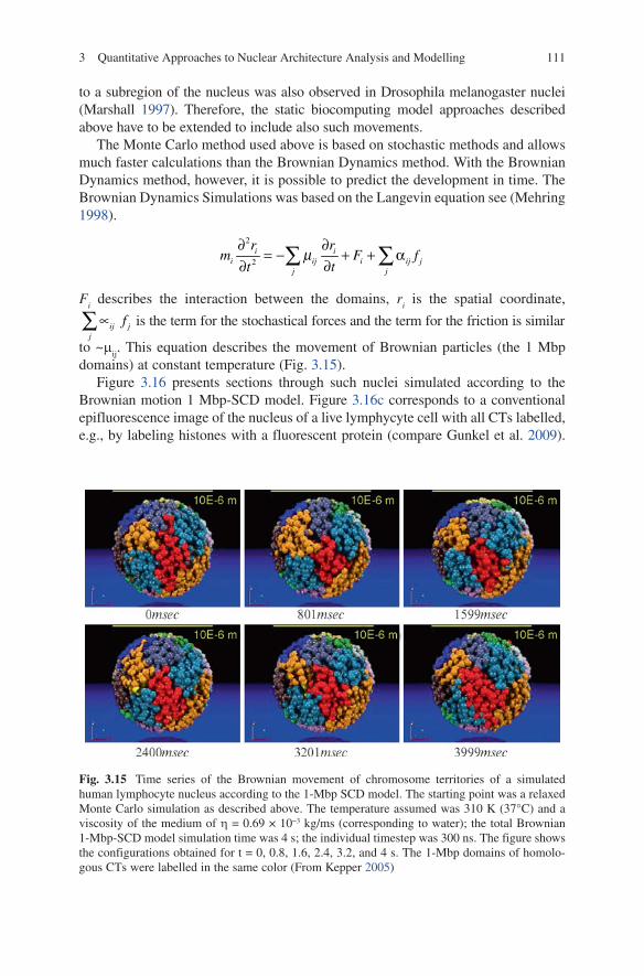
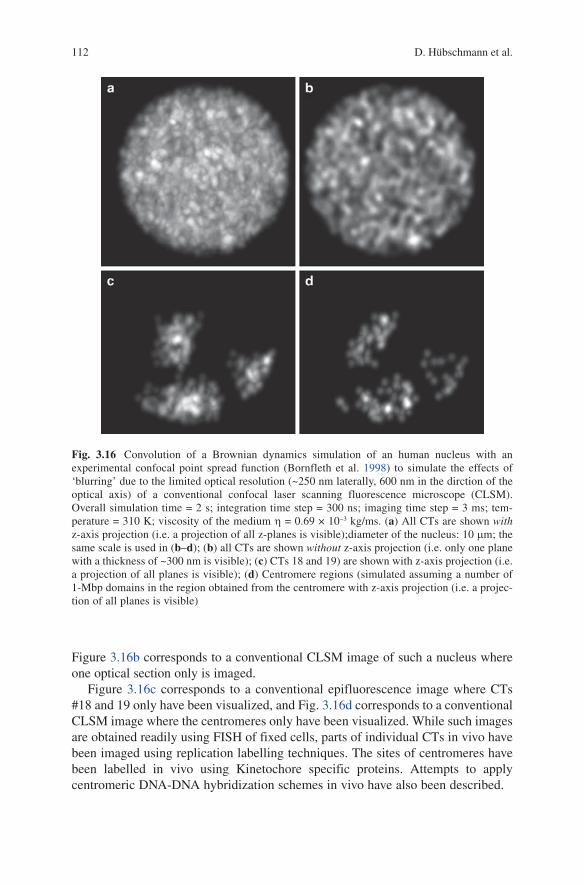
domains) at constant temperature (Fig. 3.15).Figure 3.16 presents sections through such nuclei simulated according to the
Brownian motion 1 Mbp-SCD model. Figure 3.16c corresponds to a conventional epifluorescence image of the nucleus of a live lymphycyte cell with all CTs labelled, e.g., by labeling histones with a fluorescent protein (compare Gunkel et al. 2009).
Fig. 3.15 Time series of the Brownian movement of chromosome territories of a simulated human lymphocyte nucleus according to the 1-Mbp SCD model. The starting point was a relaxed Monte Carlo simulation as described above. The temperature assumed was 310 K (37°C) and a viscosity of the medium of h = 0.69 × 10⁻³ kg/ms (corresponding to water); the total Brownian 1-Mbp-SCD model simulation time was 4 s; the individual timestep was 300 ns. The figure shows the configurations obtained for t = 0, 0.8, 1.6, 2.4, 3.2, and 4 s. The 1-Mbp domains of homolo-gous CTs were labelled in the same color (From Kepper 2005)
112 D. Hübschmann et al.
Figure 3.16b corresponds to a conventional ClSM image of such a nucleus where one optical section only is imaged.
Figure 3.16c corresponds to a conventional epifluorescence image where CTs #18 and 19 only have been visualized, and Fig. 3.16d corresponds to a conventional ClSM image where the centromeres only have been visualized. While such images are obtained readily using FISH of fixed cells, parts of individual CTs in vivo have been imaged using replication labelling techniques. The sites of centromeres have been labelled in vivo using Kinetochore specific proteins. Attempts to apply centromeric DNA-DNA hybridization schemes in vivo have also been described.
Fig. 3.16 Convolution of a Brownian dynamics simulation of an human nucleus with an experimental confocal point spread function (Bornfleth et al. 1998) to simulate the effects of ‘blurring’ due to the limited optical resolution (~250 nm laterally, 600 nm in the dirction of the optical axis) of a conventional confocal laser scanning fluorescence microscope (ClSM). Overall simulation time = 2 s; integration time step = 300 ns; imaging time step = 3 ms; tem-perature = 310 K; viscosity of the medium h = 0.69 × 10⁻³ kg/ms. (a) All CTs are shown with z-axis projection (i.e. a projection of all z-planes is visible);diameter of the nucleus: 10 mm; the same scale is used in (b–d); (b) all CTs are shown without z-axis projection (i.e. only one plane with a thickness of ~300 nm is visible); (c) CTs 18 and 19) are shown with z-axis projection (i.e. a projection of all planes is visible); (d) Centromere regions (simulated assuming a number of 1-Mbp domains in the region obtained from the centromere with z-axis projection (i.e. a projec-tion of all planes is visible)
1133 Quantitative Approaches to Nuclear Architecture Analysis and Modelling
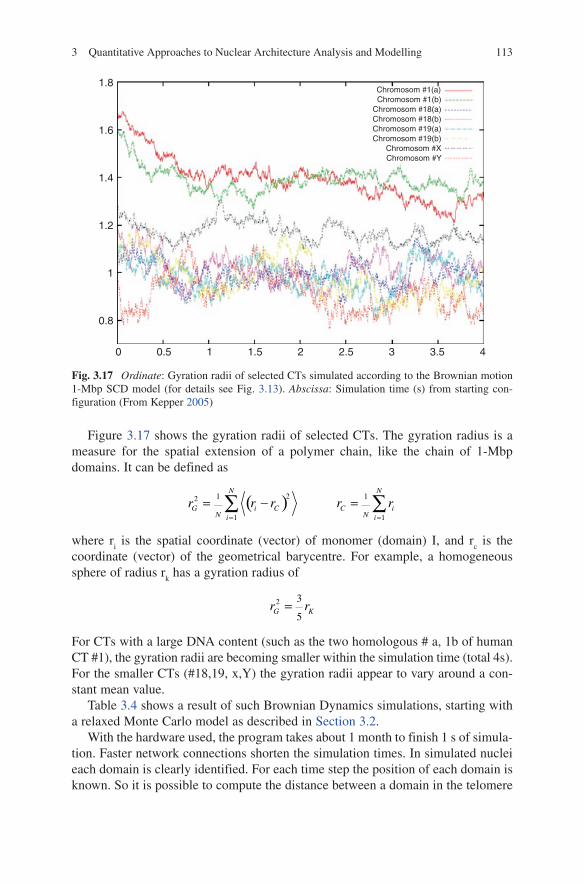
Figure 3.17 shows the gyration radii of selected CTs. The gyration radius is a measure for the spatial extension of a polymer chain, like the chain of 1-Mbp domains. It can be defined as
( )22
1 1
1 1N N
G i C C ii iN N
r r r r r= =
= − =∑ ∑
where ri is the spatial coordinate (vector) of monomer (domain) I, and r
c is the
coordinate (vector) of the geometrical barycentre. For example, a homogeneous sphere of radius r
k has a gyration radius of
2 3
5G Kr r=
For CTs with a large DNA content (such as the two homologous # a, 1b of human CT #1), the gyration radii are becoming smaller within the simulation time (total 4s). For the smaller CTs (#18,19, x,Y) the gyration radii appear to vary around a con-stant mean value.
Table 3.4 shows a result of such Brownian Dynamics simulations, starting with a relaxed Monte Carlo model as described in Section 3.2.
With the hardware used, the program takes about 1 month to finish 1 s of simula-tion. Faster network connections shorten the simulation times. In simulated nuclei each domain is clearly identified. For each time step the position of each domain is known. So it is possible to compute the distance between a domain in the telomere
Chromosom #1(a)Chromosom #1(b)
Chromosom #18(a)Chromosom #18(b)
Chromosom #19(b)Chromosom #19(a)
Chromosom #XChromosom #Y
0.8
0 0.5 1 1.5 2 2.5 3 3.5 4
1
1.2
1.4
1.6
1.8
Fig. 3.17 Ordinate: Gyration radii of selected CTs simulated according to the Brownian motion 1-Mbp SCD model (for details see Fig. 3.13). Abscissa: Simulation time (s) from starting con-figuration (From Kepper 2005)
114 D. Hübschmann et al.
and in the centromere region. To show the differences between the time steps the mean value and the standard deviation are calculated. In Table 3.4, the sizes for the chromosomes 1, 18, 19 and Y are given. The size of the chromosome does not cor-relate with the distance between the domain in the telomere and the centromere region. Centromere regions are not in the “middle” of chromosomes, there are two different arms with different lengths. The ratio differs with the chromosomes and is specific for the chromosome type.
3.8 Towards Quantitative Analysis of Nuclear Genome Nanostructure I: Computer Models
It is obvious that in real nuclei the 1 Mbp-domains of the SCD model cannot be spheres. This assumption simply means that the very complex ‘nanostructure’ of the chromatin inside the individual domains was not regarded. This deliberate oversim-plification may be justified as long as the large scale nuclear genome architecture is considered, such as the general arrangement of chromosome territories in the nucleus, or even the mean distances between telomeres and centromere domains. However, spatial constraints of functional nuclear genome architecture, such as rep-lication, transcription and repair, are intimately connected with the nanostructure, i.e. with dimensions considerably smaller than the 250 nm radius of a 1-Mbp-domain, any attempt to quantitative modelling such nanostructures has to be based on ideas on the nanoscale architecture of chromatin domains. In this respect, chromatin loops of different sizes have become a common textbook scheme to explain how chromatin packaging is achieved from the DNA level to the level of entire metaphase chromo-somes. Such qualitative models need to be translated into quantitative, experimen-tally testable predictions; only in this way, the development of a consistent biophysical understanding of functional nuclear nanoarchitecture will become possible.
So far, several computer models have been proposed to numerically predict chromatin domain nanostructure up to the structure. For this, backfolding of chro-matin fibres at some level is indispensable: In models that dismiss such backfold-ing, chromatin fibres expand throughout much of the nuclear space resulting in a non-territorial/non-domain interphase chromosome organization. In the random-walk/giant-loop (RW/Gl) model, chromatin loops with a size of several megabases
Table 3.4 Simulated distances between telomere and centromere domains. A nucleus of a human cell simulated with a total time of 200 ms with Brownian Dynamics simulations; the integration time step was set to 50 ns, every 500 ms the positions of all domains were saved; the simulated tempera-ture was 310 K, the viscosity h = 0.69 · 10−3 kg m·s (Chromosome sizes were taken from Morten 1991). Telomere and Centromere domains were identified according to the centromeric index
Chromosome 1 18 19 Y
First homologue 2.5 ± 0.2 mm 1.6 ± 0.5 mm 1.2 ± 0.3 mm 2.3 ± 0.2 mmSecond homologue 1.7 ± 0.2 mm 1.8 ± 0.2 mm 1.8 ± 0.4 mmSize in Mbp 263 98 85 59
1153 Quantitative Approaches to Nuclear Architecture Analysis and Modelling
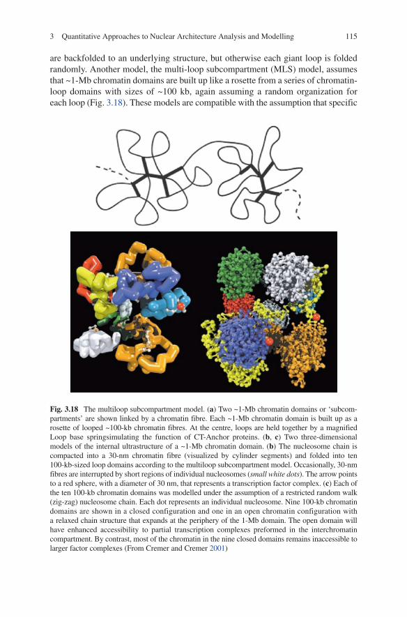
are backfolded to an underlying structure, but otherwise each giant loop is folded randomly. Another model, the multi-loop subcompartment (MlS) model, assumes that ~1-Mb chromatin domains are built up like a rosette from a series of chromatin-loop domains with sizes of ~100 kb, again assuming a random organization for each loop (Fig. 3.18). These models are compatible with the assumption that specific
Fig. 3.18 The multiloop subcompartment model. (a) Two ~1-Mb chromatin domains or ‘subcom-partments’ are shown linked by a chromatin fibre. Each ~1-Mb chromatin domain is built up as a rosette of looped ~100-kb chromatin fibres. At the centre, loops are held together by a magnified loop base springsimulating the function of CT-Anchor proteins. (b, c) Two three-dimensional models of the internal ultrastructure of a ~1-Mb chromatin domain. (b) The nucleosome chain is compacted into a 30-nm chromatin fibre (visualized by cylinder segments) and folded into ten 100-kb-sized loop domains according to the multiloop subcompartment model. Occasionally, 30-nm fibres are interrupted by short regions of individual nucleosomes (small white dots). The arrow points to a red sphere, with a diameter of 30 nm, that represents a transcription factor complex. (c) Each of the ten 100-kb chromatin domains was modelled under the assumption of a restricted random walk (zig-zag) nucleosome chain. Each dot represents an individual nucleosome. Nine 100-kb chromatin domains are shown in a closed configuration and one in an open chromatin configuration with a relaxed chain structure that expands at the periphery of the 1-Mb domain. The open domain will have enhanced accessibility to partial transcription complexes preformed in the interchromatin compartment. By contrast, most of the chromatin in the nine closed domains remains inaccessible to larger factor complexes (From Cremer and Cremer 2001)
116 D. Hübschmann et al.
positions of genes inside or outside a chromatin-loop domain are not required for activation or silencing. However, they do make different predictions: first, about the extent of intermingling of different giant chromatin loops and chromatin-loop rosettes; and second, about the interphase distances between genes and other DNA segments that are located along a given chromosome.
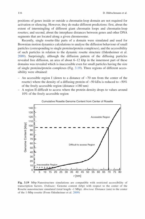
Recently, single rosette-like parts of a domain were simulated and used for Brownian motion dynamics calculations to analyse the diffusion behaviour of small particles (corresponding to single proteins/protein complexes), and the accessibility of such particles in relation to the dynamic rosette structure (Odenheimer et al. 2009). Surprisingly, although the diffusion pattern of the diffusing particles revealed free diffusion, an area of about 6–12 kbp in the innermost part of these domains was revealed which is inaccessible even for small particles having the size of single proteins/protein complexes (Fig. 3.19). Three regions of different acces-sibility were obtained:
An accessible region I (down to a distance of ~70 nm from the center of the –rosette) where the density of a diffusing protein of ~50 kDa is reduced to ~50% of the freely accessible region (distance >180 nm)A region II difficult to access where the protein density drops to values around –10% of the freely accessible region
Cumulative Rosette Genome Content from Center of Rosette
Difficult to access Region
Inaccessible Region
r [nm]0
0
10
20
30
40
50
60
70
80
90
100
110
120
130
140
5 10 15 20 25 30 35 40 45 50 55 60 65 70 75 80
Accessible Region
Gen
ome
Con
tent
[kbp
]
Fig. 3.19 Mbp-Nanostructure simulations are compatible with restricted accessibility of transcription factors. Ordinate: Genome content (kbp) with respect to the center of the Rosette nanostructure simulated (total length ~1 Mbp). Abscissa: Distance (nm) to the center of the 1-Mbp rosette (From Odenheimer et al. 2009)
1173 Quantitative Approaches to Nuclear Architecture Analysis and Modelling
An in-accessible region III of about 3 kbp in length and a radius r –limit
= 20 nm where the relative protein density drops to very small densities (in the simula-tions to zero)
It is tempting to assume that a localisation of a promotor sequence in this area might silence the respective gene by the physical inaccessibility of this area for transcription factors: Thus, the RNA polymerase may not bind and the entire gene may not be transcribed. Thus, the silencing of genes in a chromatin domain could possibly be caused solely by physical inaccessibility. These predictions are well compatible with the findings of Verschure et al. (2003) based on conventional light microscopy observations.
3.9 Towards Quantitative Analysis of Nuclear Genome Nanostructure II: Perspectives of Superresolution Light Microscopy
As Fig. 3.20 indicates, in a conventional light microscopic observation volume corre-sponding to ~250 × 250 × 600 nm3 , a region with a diameter of 2 × r
limit = 2 × 20 nm =
40 nm was predicted to be inaccessible; this is only about 0.2% of the minimal conventional observation volume. Such a small region of inaccessibility is far below the detection limits of conventional light microscopy. Consequently, due to this lack of optical resolution the prediction of very small regions of inaccessibility in the range of few tens of nanometer is well compatible with the experimental results of tracking experiments of single streptavidin molecules in structurally and functionally distinct nuclear compartments. These conventional microscopy observations indicated that all nuclear subcompartments were easily and similarly accessible for such an average-sized protein, and even condensed heterochromatin neither excluded single molecules nor impeded their passage (Gruenwald et al. 2008). However, these protein molecules did not accumulate in heterochromatin, suggesting comparatively less free volume.
While the predictions of the nanostructure model presented are thus fully com-patible with available conventional light microscopy data, a test of the predictions of this and other nanostructure models concerning small regions of inaccessibility requires microscopic techniques with an effective resolution in the range of few tens of nanometer. Until a few years ago, such a resolution was available only with electron microscopy (EM) approaches while for far field flight microscopy, such a resolution was regarded to be impossible to achieve.
Since the famous publication of Ernst Abbe (1873), this limit was regarded to be due to the wave nature of light and thus unsurmountable. Based on the diffraction theory of light, Ernst Abbe postulated for a specific color a “specific smallest distance which never can significantly surpass half a wavelength of blue light”, i.e. about 200 nm. A very similar conclusion was obtained in 1896 by lord Rayleigh, “tracing the image representative of a mathematical point in the object, the point being regarded as self-luminous. The limit to definition depends upon the
118 D. Hübschmann et al.
fact that owing to diffraction the image thrown even by a perfect lens ids not confined to a point, but distends itself over a patch or disk of light of finite diameter” Rayleigh (1896). From this, Rayleigh concluded “that the smallest resolvable distance e is given by e = ½ l/sina, a being the wave-length in the medium where the object is situated, and a the divergence-angle of the extreme ray (the semi-angular aperture) in the same medium”. Thus the same lightoptical (lateral) resolution limit of ca. 200 nm (for abbreviation often called ‘Abbe-limit’) is obtained in both theories.
Recently, however, a variety of laseroptical far field microscopy techniques based on fluorescence excitation has been developed to overcome the Abbe-limit of 200 nm at least in one direction, and to make possible light Optical Analysis of BioStructures by Enhanced Resolution (“lOBSTER”). Some well known lOBSTER methods are confocal 4Pi-laser Scanning Microscopy (Cremer and Cremer 1978; Hell and Wichmann 1994; Hell 2003; Egner et al. 2002, Bewersdorf et al. 2006, Baddeley et al. 2006, SMI microscopy (Hildenbrand et al. 2005; Martin et al. 2004) structured/patterned illumination microscopy (Heintzmann and Cremer 1999), STED micros-copy (Hell and Wichmann 1994; Hell 2007; Schmidt et al. 2008; Donnert et al. 2006) or localization microscopy approaches using far field fluorescence micros-copy (Cremer et al. 1996; Patwardhan 1997; Bornfleth et al. 1998; van Oijen et al. 1999; Edelmann et al. 1999; Esa et al. 2000; lacoste et al. 2000; Schmidt et al. 2008; Heilemann et al. 2002; Betzig et al. 2006; Hess et al. 2006; Egner et al. 2002; Reymann et al. 2008; lemmer et al. 2008). Using these latter techniques, an effec-tive optical resolution in the 10–20 nm regime has been obtained. For the first time,
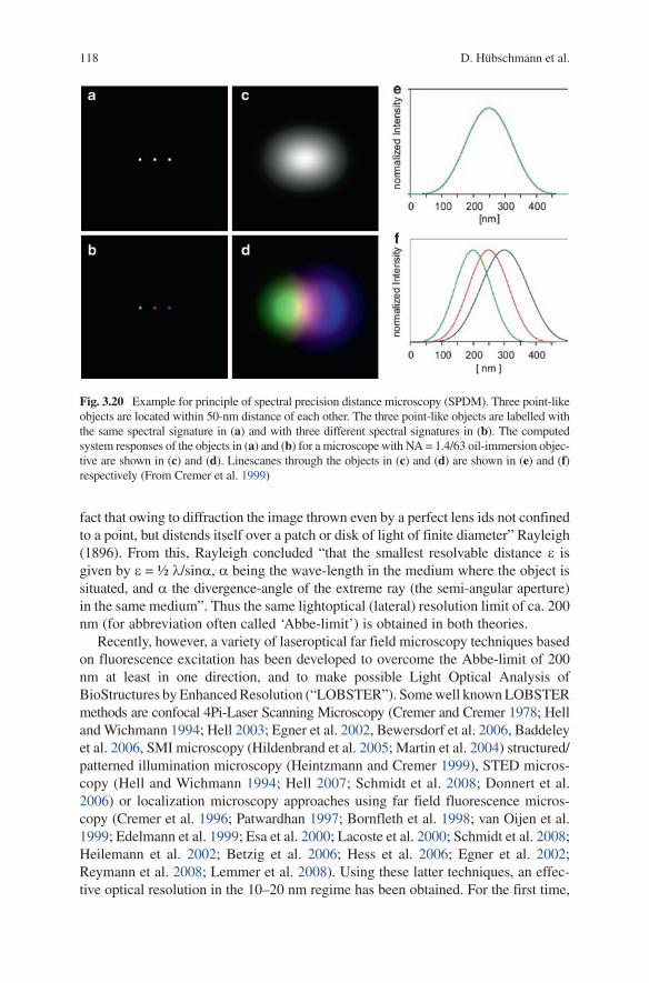
Fig. 3.20 Example for principle of spectral precision distance microscopy (SPDM). Three point-like objects are located within 50-nm distance of each other. The three point-like objects are labelled with the same spectral signature in (a) and with three different spectral signatures in (b). The computed system responses of the objects in (a) and (b) for a microscope with NA = 1.4/63 oil-immersion objec-tive are shown in (c) and (d). linescanes through the objects in (c) and (d) are shown in (e) and (f) respectively (From Cremer et al. 1999)
1193 Quantitative Approaches to Nuclear Architecture Analysis and Modelling
this allowed “nanoimaging” of biostructures at macromolecular resolution using fluorescence excitation by visible light. While STED microscopy is a focused beam method allowing to rapidly image small regions of interest (few mm extension), the complementary “spectrally assigned localization microscopy” (SAlM) techniques are preferentially used in non-focusing setups, thus allowing to rapidly image large regions of interest (50–100 mm extension).
The basis of SAlM as a far field fluorescence microscopy “nanoimaging” approach using biocompatible temperature conditions is the independent localiza-tion of ‘point like’ objects excited to fluorescence emission by a focused laser beam or by non-focused illumination by ‘optical isolation’, i.e. the localization is assigned by appropriate spectral features. This approach, called by us ‘spectral precision microscopy’ (SPM) or spectral precision distance/position determination microscopy (SPDM) was conceived and realized in proof-of-principle experiments already in the 1990s (Cremer et al. 1996; Bornfleth et al. 1998; Cremer et al. 1999; Esa et al. 2000, 2001; Edelmann et al. 2000).
The principle of SPDM/SAlM is shown schematically in Fig. 3.20. let us assume three closely neighboring targets in a cell to be studied with distances much smaller than 1 FWHM, where FWHM represents the Full-Width-at-Half-Maximum of the effective Point Spread Function (PSF) of the optical system used. The ‘point-like’ (diameter much smaller than 1 FWHM) targets t
1, t
2 and t
3 (e.g., three molecules) are
assumed to have been labeled with three different fluorescent spectral signatures specs1, specs2 and specs3. For example, t
1 is labeled with specs1, t
2 with specs2
and t3 with specs3. The registration of the images (using focused or non-focused
optical devices with a given FWHM) is performed in a spectrally discriminated way so that in a first image stack IM1, a specs1 intensity value I1 is assigned to each voxel v
k (k = 1,2,3,…) of the object space; in a second image stack IM2, a specs2 intensity
value I2 is assigned to each voxel vk of the object space; and in a third 3-D image
stack IM3, a specs3 intensity value I3 is assigned to each voxel vk of the object
space. The positions of the objects/molecules obtained are assigned to a position map. Early ‘proof-of-principle’ experiments using confocal laser scanning fluores-cence microscopy (ClSM) at room temperature to determine the positions (xyz) and mutual Euclidean distances of small sites on the same DNA molecule labelled with three different spectral signatures yielded a lateral effective resolution of about 30 nm (ca. 1/16th of the wavelength used) and ca. 50 nm axial effective resolution (Esa et al. 2000): Sites with a 3D distance of only 50 nm were still discriminated; their (xyz) positions were determined independently from each other with an error of few tens of nanometer, including the correction for optical aberrations. It was noted “that the SPM (Spectral Precision Microscopy = SPDM) strategy can be applied to more than two or three closely neighbored targets, if the neighboring targets t
1, t
2, t
3, …, t
n have
sufficiently different spectral signatures specs1, specs2,…specsn…. Three or more spectral signatures allow true structural conclusions…. Furthermore, it is clear that essentially the same SPM strategy can be applied also in all cases where the distance between targets of the same spectral signature is larger than FWHM. Computer simu-lations performed by (Bornfleth et al. 1998) indicated that a distance of about 1.5 FWHM is sufficient.” (Cremer et al. 1999). Compared with related concepts (Betzig et al. 2006, van Oijen et al. 1999), in the SPDM approach the focus of application was
120 D. Hübschmann et al.
to (a) to perform superresolution analysis by the direct evaluation of the positions of the spectrally separated objects; (b) to adapt the method to far field fluorescence microscopy at temperatures in the 300 K range (“room temperature”); (c) to specify spectral signatures to include all kinds of fluorescent emission parameters suitable, from absorption/emission spectra to fluorescence life times (Heilemann et al. 2002) to any other method allowing ‘optical isolation’ (Cremer et al. 2001 US Patent 7,298,461 B2) . Optical isolation means that at a given time and registration mode, the distance between two objects/molecules is larger than the FWHM. Early concepts included even the use of photoswitching to molecules from a state A to a state B in an observation volume in a reversible or irreversible way to improve the gain of nanostructural information (Cremer and Cremer 1972 DE).
In the last few years, approaches based on principles of SPDM and related methods (‘spectrally assigned localization microscopy‘, SAlM) have been consid-erably improved by several groups, especially by using photoswitchable fluoro-chromes. By imaging fluorescent bursts of single molecules after light activation, the position of the molecules was determined with a precision significantly better than the FWHM. These microscopic techniques were termed photoactivated local-ization microscopy (PAlM) (Betzig et al. 2006), fluorescence photoactivation localization microscopy (FPAlM) (Hess et al. 2006), stochastic optical reconstruc-tion microscopy (STORM) (Rust et al. 2006) or PAlM with independently running acquisition (PAlMIRA) (Geisler et al. 2007, Andresen et al. 2008). In all these approaches, special fluorochromes were used which can be photoswitched between a ‘dark’ state A and a ‘bright’ state B (Hell Nature Biotech 2003).
Recently, we applied SPDM in the nanometer resolution scale to conventional fluo-rochromes that show “reversible photobleaching” or “blinking”. “Reversible photo-bleaching” has been shown to be a general behavior in several fluorescent proteins, e.g., CFP, Citrine or eYFP (15–18). In such cases, the fluorescence emission of certain types can be described by assuming three different states of the molecule: A fluorescent state M
fl; a reversibly bleached state M
rbl; and an irreversibly bleached stat M
ibl. In the M
rbl
state, the molecule can be excited to a large number of times to the Mfl state (fluorescence
burst) until it passes into the irreversibly bleached state (i.e. a dark state long compared with the time required for a burst of fluorescence photons); and thus its position be determined. With velocity constants k
1, k
2, k
3 one can assume the transition scheme
2
3
1
kk
rbl fl iblk
M M M→
→←
We recently showed that reversible photobleaching can be used for superresolution imaging (SPDM
Phymod) of cellular nanostructures labeled with conventional fluoro-
chromes such as Alexa 488 (Reymann et al. 2008; Baddeley et al. 2009) or the Green Fluorescent Protein variant YFP (lemmer et al. 2008). This novel extensions of the SPDM approach are based on the possibility to produce the optical isolation required by allowing only one molecule in a given observation volume to be in the M
rbl–M
fl cycle. In this case, each stochastic time onset (t
1,t
2,t
3,…t
k) of a fluores-
cence burst is regarded to represent a specific PHYMOD spectral signature
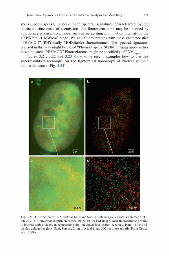
1213 Quantitative Approaches to Nuclear Architecture Analysis and Modelling
specs1,specs2,specs3,…specsk. Such spectral signatures characterized by the stochastic time onset of a emission of a fluorescent burst may be obtained by appropriate physical conditions, such as an exciting illumination intensity in the 10 kW/cm2–1 MW/cm2 range. We call fluorochromes with these characteristics “PHYMOD” (PHYsically MODifiable) fluorochromes. The spectral signatures realized in this way might be called “Phymod”specs. SPDM imaging appreoaches based on such “PHYMOD” Fluorochromes might be specified as SPDM
Phymod.
Figures 3.21, 3.22 and 3.23 show some recent examples how to use this superresolution technique for the lightoptical nanoscopy of nuclear genome nanoarchitecture (Fig. 3.24).
Fig. 3.21 Distribution of H2A proteins (red) and Snf2H proteins (green) within a human U2OS nucleus. (a) Conventional epifluorescence image. (b) 2ClM image, each fluorochrome-position is blurred with a Gaussian representing the individual localization accuracy. Panel (c) and (d) display enlarged regions. Scale bars are 2 mm in A and B and 500 nm in (c) and (d) (From Gunkel et al. 2009)
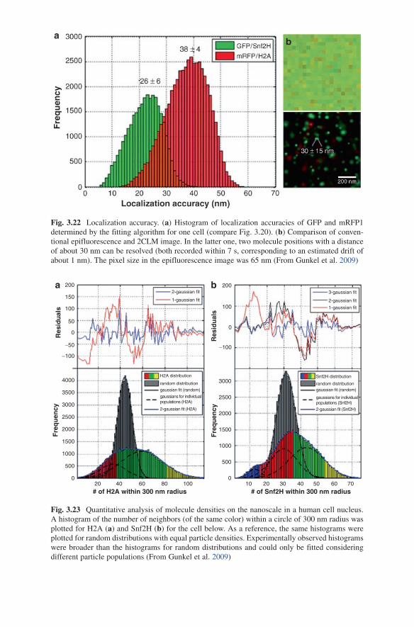
Fig. 3.22 localization accuracy. (a) Histogram of localization accuracies of GFP and mRFP1 determined by the fitting algorithm for one cell (compare Fig. 3.20). (b) Comparison of conven-tional epifluorescence and 2ClM image. In the latter one, two molecule positions with a distance of about 30 nm can be resolved (both recorded within 7 s, corresponding to an estimated drift of about 1 nm). The pixel size in the epifluorescence image was 65 nm (From Gunkel et al. 2009)
2-gaussian fit 3-gaussian fit
2-gaussian fit
2-gaussian fit (Snf2H)2-gaussian fit (H2A)
020 40 60 80 100 10 20 30 40 50 60 70
0
500500
10001000
1500
15002000
20002500
25003000
3000
3500
4000
Fre
qu
ency
Res
idu
als
Fre
qu
ency
# of H2A within 300 nm radius
a b
# of Snf2H within 300 nm radius
Res
idu
als
00
50
100 100
150
200 200
−100
−100−50
1-gaussian fit
Snf2H distributionH2A distribution
random distributionrandom distributiongaussian fit (random)gaussian fit (random)
gaussians for individualpopulations (Snf2H)
gaussians for individualpopulations (H2A)
1-gaussian fit
Fig. 3.23 Quantitative analysis of molecule densities on the nanoscale in a human cell nucleus. A histogram of the number of neighbors (of the same color) within a circle of 300 nm radius was plotted for H2A (a) and Snf2H (b) for the cell below. As a reference, the same histograms were plotted for random distributions with equal particle densities. Experimentally observed histograms were broader than the histograms for random distributions and could only be fitted considering different particle populations (From Gunkel et al. 2009)
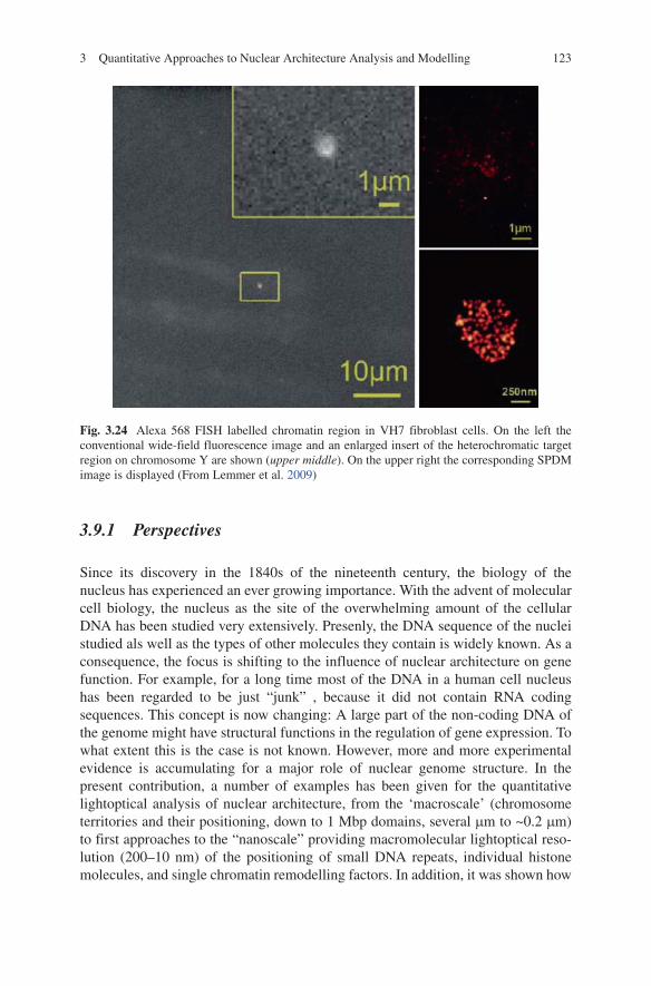
1233 Quantitative Approaches to Nuclear Architecture Analysis and Modelling
3.9.1 Perspectives
Since its discovery in the 1840s of the nineteenth century, the biology of the nucleus has experienced an ever growing importance. With the advent of molecular cell biology, the nucleus as the site of the overwhelming amount of the cellular DNA has been studied very extensively. Presenly, the DNA sequence of the nuclei studied als well as the types of other molecules they contain is widely known. As a consequence, the focus is shifting to the influence of nuclear architecture on gene function. For example, for a long time most of the DNA in a human cell nucleus has been regarded to be just “junk” , because it did not contain RNA coding sequences. This concept is now changing: A large part of the non-coding DNA of the genome might have structural functions in the regulation of gene expression. To what extent this is the case is not known. However, more and more experimental evidence is accumulating for a major role of nuclear genome structure. In the present contribution, a number of examples has been given for the quantitative lightoptical analysis of nuclear architecture, from the ‘macroscale’ (chromosome territories and their positioning, down to 1 Mbp domains, several mm to ~0.2 mm) to first approaches to the “nanoscale” providing macromolecular lightoptical reso-lution (200–10 nm) of the positioning of small DNA repeats, individual histone molecules, and single chromatin remodelling factors. In addition, it was shown how
Fig. 3.24 Alexa 568 FISH labelled chromatin region in VH7 fibroblast cells. On the left the conventional wide-field fluorescence image and an enlarged insert of the heterochromatic target region on chromosome Y are shown (upper middle). On the upper right the corresponding SPDM image is displayed (From lemmer et al. 2009)
124 D. Hübschmann et al.
structural information can be integrated into quantitative models of nuclear genome organisation and used to predict medically important consequences, such as the formation of cancer correlated chromosome translocations induced by ionizing radiation. It is anticipated that the new possibilties of lightoptical superresolution microscopy (‘nanoscopy’) and their correlation with ultrastructural methods, e.g., transmission electron microscopy (EM), Scanning EM (SEM), cryo-electron tomography, focused ion beam SEM, or X-ray microscopy will allow to gain nano-structural information until recently thought to be beyond the possibilities of experimental research. The integration of this knowledge into numerical models of nuclear structure down to the level of the nucleosomes will eventually make possible to develop a “virtual cell nucleus”. This is expected to contribute substantially to a deeper insight into the basic understanding of life but also allow predictions valu-able for cellular reprogramming and the effect of specific therapeutic agents.
Acknowledgements This work was supported by grants from the Deutsche Forschungsge-meinschaft and the European Union. For discussions and other help we especially thank Manuel Gunkel, Rainer Kaufmann and Thomas Cremer.
References
Abbe E (1873) Beitraege zur Theorie des Mikroskops und der mikroskopischen Wahrnehmung. Arch Mikrosk Anat 9:411–468
Albiez H, Cremer M, Tiberi C, Vecchio l, Schermelleh l, Dittrich S, Kuepper K, Joffe B, Thormeyer T, von Hase J, Yang S, Rohr K, leonhardt H, Solovei I, Cremer C, Fakan S, Cremer T (2006) Chromatin domains and the interchromatin compartment form structurally defined and functionally interacting nuclear networks. Chromosome Res 14:707–733
Andresen M, Stiel AC, Folling J, Wenzel D, Schonle A, Egner A et al (2008) Photoswitchable fluorescent proteins enable monochromatic multilabel imaging and dual color fluorescence nanoscopy. Nat Biotechnol 26:1035–1040
Arsuaga J, Greulich-Bode KM, Vazquez M, Bruckner M, Hahnfeldt P, Brenner DJ, Sachs R, Hlatky l (2004) Chromosome spatial clustering inferred from radiogenic aberrations. Int J Radiat Biol 80:507–515
Baddeley D, Carl C, Cremer C (2006) 4Pi microscopy deconvolution with a variable point-spread function. Appl Opt 45:7056–7064
Baddeley D, Jayasinghe I, Cremer C, Cannell M, Soeller C (2009) light-induced dark states of organic fluochromes enable 30 nm resolution imaging in standard media. Biophys J. doi:10.1016/j.bpj.2008.11.002
Ballarini F, Biaggi M, Ottolenghi A (2002) Nuclear architecture and radiation induced chromo-some aberrations: models and simulations. Radiat Prot Dosimetry 99:175–182
Betzig E, Patterson GH, Sougrat R, lindwasser OW, Olenych S, Bonifacino JS, Davidson MW, lippincott-Schwartz J, Hess HF (2006) Imaging intracellular fluorescent proteins at nanome-ter resolution. Science 313:1642–1645
Bewersdorf J, Bennett BT, Knight Kl (2006) H2AX chromatin structures and their response to DNA damage revealed by 4Pi microscopy. Proc Natl Acad Sci U S A 103:18137–18142
Bolzer A, Kreth G, Solovei I, Koehler D, Saracoglu K, Fauth Ch, Müller S, Eils R, Cremer C, Speicher M, Cremer T (2005) Three-dimensional maps of all chromosomes in human male fibroblast nuclei and prometaphase rosettes. PlOS Biol 3:e157
Bornfleth H, Sätzler K, Eils R, Cremer C (1998) High–precision distance measurements and volume–conserving segmenta tion of objects near and below the resolution limit in three–dimensional confoca l fluorescence microscopy. J Microsc 189:118–136
1253 Quantitative Approaches to Nuclear Architecture Analysis and Modelling
Bornfleth H, Edelmann P, Zink D, Cremer C (1999a) Handbook of computer vision and applications, vol III, Chapter Three – dimensional analysis of genome topology. Academic Press, San Diego/New York, pp 859–878
Bornfleth H, Edelmann P, Zink D, Cremer T, Cremer C (1999b) Quantitative motion analysis of sub–chromosomal foci in living cells using four–dimensional microscopy. Biophys J 75(5):2871–2886
Boyle S, Gilchrist S, Bridger JM, Mahy Nl, Ellis JA, Bickmore WA (2001) The spatial organiza-tion of human chromosomes within the nuclei of normal and emerin-mutant cells. Hum Mol Genet 10:211–219
Branco MR, Pombo A (2007) Chromosome organization: new facts, new models. Trends Cell BiolBridger JMl (1999) Analysis of mammalian interphase chromosome by FISH and immunofluo-
rescence. In: Bickmore WA (ed) Chromsome structural ananlysis. Oxford University Press, Oxford, pp 103–123
Chevret E, Volpi EV, Sheer D (2000) Mini review: form and function in the human interphase chromosome. Cytogenetic Cell Genet 90(1–2):13–21
Cornforth MN, Greulich-Bode KM, loucas BD, Arsuaga J, Vazquez M, Sachs RK, Bruckner M, Molls M, Hahnfeldt P, Hlatky l, Brenner DJ (2002) Chromosomes are predominantly located randomly with respect to each other in interphase human cells. J Cell Biol 159:237–244
Cremer C, Cremer T (1972) Verfahren zur Darstellung bzw. Modifikation von Objekt-Details, deren Abmessungen außerhalb der sichtbaren Wellenlänge liegen (Procedure to image or modify object details with dimensions below the wavelength of visible light). Ger Pat Appl P 21 16 521.9 (filed 5 April 1971)
Cremer C, Cremer T (1978) Considerations on a laser-Scanning-Microscope with high resolution and depth of field. Microsc Acta 81:31–44
Cremer T (1985) Von der Zellenlehre zur Chromosomentheorie, Naturwissenschaftliche Erkenntnis und Theorienwechsel in der fr¨uhen Zell– und Vererbungsforschung. Springer, Heidelberg
Cremer T, Kurz A, Zirbel R, Dietzel S, Rinke B, Schröck E, Speicher MR, Mathieu U, Jauch A, Emmerich P, Scherthan H, Ried T, Cremer C, lichter P (1993) Role of chromosome territories in the functional compartmentalization of the cell nucleus. Cold Spring Harb Symp Quant Biol 85:777–792
Cremer T, lichter P, Borden J, Ward DC, Manuelidis l (1988) Detection of chromosome aberra-tions in metaphase and interphase tumor cells by in situ hybridization using chromosome–specific library probes. Hum Genet 80:235–246
Cremer T, Kurz A, Zirbel R, Dietzel S, Rinke B, Schröck E, et al. (1993) Role of chromosome territories in the functional compartmentalization of the cell nucleas. Cold Spring Harb Symp Quant Biol. 1993;85:777–792
Cremer C, Muenkel C, Granzow M, Jauch A, Dietzel S, Eils R, Guan XY, Meltzer PS, Trent JM, langowski J, Cremer T (1996) Nuclear architecture and the induction of chromosomal aber-rations. Mutat Res 366:97–116
Cremer C, Edelmann P, Bornfleth H, Kreth G, Muench H, luz H, Hausmann M (1999) Principles of Spectral Precision Distance confocal microscopy for the analysis of molecular nuclear structure. In: Jähne B, Haußecker H, Geißler P (eds) Handbook of computer vision and appli-cations, vol 3. Academic Press, San Diego/New York, pp 839–857
Cremer T, Kreth G, Koester H, Fink RH, Heintzmann R, Cremer M, Solovei I, Zink D, Cremer C (2000) Chromosome territories, interchromatin domain compartment, and nuclear matrix: an integrated view of the functional nuclear architecture. Crit R Eukaryot Gene Express 12:179–212
Cremer M, Hase JV, Volm T, Brero A, Kreth G, Walter J, Fischer C, Solovei I, Cremer C, Cremer T (2001) Non-random radial higher-order chromatin arrangements in nuclei of diploid human cells. Chrom Res 9:541–567
Cremer T, Cremer C (2001) Chromosome territiories, nuclear architecture and gene regulation in mammalian cells. Nat Rev Genet 2(4):292–301
Cremer M, Kupper K, Wagler B, Wizelman l, von Hase J, Weiland Y, Kreja l, Diebold J, Speicher MR, Cremer T (2003) Inheritance of gene density-related higher order chromatin arrangements in normal and tumor cell nuclei. J Cell Biol 162:809–820
126 D. Hübschmann et al.
Cremer T, Cremer M, Dietzel S, Mueller S, Solovei I, Fakan S (2006) Chromosome territories – a functional nuclear landscape. Curr Opin Cell Biol 18:307–316
Cremer T, Cremer C (2006a) Rise, fall and resurrection of chromosome territories: a historical perspective. Part I. The rise of chromosome territories. Eur J Histochem 50:161–176
Cremer T, Cremer C (2006b) Rise, fall and resurrection of chromosome territories: a historical perspective. Part II. Fall and resurrection of chromosome territories during the 1950s to 1980s. Part III. Chromosome territories and the functional nuclear architecture: experiments and models from the 1990s to the present. Eur J Histochem 50:223–272
Croft JA, Bridger JM, Boyle S, Perry P, Teague P, Bickmore WA (1999) Differences in the locali-sation and morphology of chromosomes in the human nucleus. J Cell Biol 145:1119–1131
Dietzel S, Eils R, Saetzler K, Bornfleth H, Jauch A, Cremer C, Cremer T (1998) Evidence against a looped structure of the inactive human X–chromosome territory. Exp Cell Res 240:187–196
Dimitrova DS, Berezney R (2002) The spatio-temporal organization of DNA replication sites is iden-tical in primary, immortalized and transformed mammalian cells. J Cell Sci 115:4037–4051
Donnert G, Keller J, Medda R, Andrei MA, Rizzoli S, luhrmann R, Jahn R, Eggeling C, Hell SW (2006) Macromolecular–scale resolution in biological fluorescence microscopy. Proc Natl Acad Sci U S A 103:11440–11445
Deloukas P, Schuler GD, Gyapay G, Beasley EM, Soderlund C, Rodriguez-Tomé P, Hui l, Matise TC, McKusick KB, Beckmann JS, Bentolila S, Bihoreau M, Birren BB, Browne J, Butler A, Castle AB, Chiannilkulchai N, Clee C, Day PJ, Dehejia A, Dibling T, Drouot N, Duprat S, Fizames C, Fox S, Gelling S, Green l, Harrison P, Hocking R, Holloway E, Hunt S, Keil S, lijnzaad P, louis-Dit-Sully C, Ma J, Mendis A, Miller J, Morissette J, Muselet D, Nusbaum HC, Peck A, Rozen S, Simon D, Slonim DK, Staples R, Stein lD, Stewart EA, Suchard MA, Thangarajah T, Vega-Czarny N, Webber C, Wu X, Hudson J, Auffray C, Nomura N, Sikela JM, Polymeropoulos MH, James MR, lander ES, Hudson TJ, Myers RM, Cox DR, Weissenbach J, Boguski MS, Bentley DR (1998) A physical map of 30, 000 human genes. Science 282:744–746
Dundr M, Misteli T (2001) Functional architecture in the cell nucleus. Biochem J 356:297–310Edelmann P, Bornfleth H, Zink D, Cremer T, Cremer C (2001) Morphology and dynamics of
chromosome territories in living cells. Biochimica et Biophysica Acta 1551:M29–M40Edelmann P, Cremer C (2000) Improvement of confocal spectral precision distance microscopy
(SPDM). In: Farkas Dl, leif RC (eds) Optical diagnostics of living Cells III. Proceedings of SPIE, vol 3921, pp 313–320
Edelmann P, Esa A, Hausmann M, Cremer C (1999) Confocal laser-scanning fluorescence micros-copy: in situ determination of the confocal point-spread function and the chromatic shifts in intact cell nuclei. Optik 110:194–198
Edwards AA (1997) The use of chromosomal aberrations in human lymphocytes for biological dosimetry. Radiat Res 148:539–544
Egner A, Jakobs S, Hell SW (2002) Fast 100-nm resolution three-dimensional microscope reveals structural plasticity of mitochondria in live yeast. Proc Natl Acad Sci U S A 99:3370–3375
Esa A, Edelmann P, Trakthenbrot l, Amariglio N, Rechavi G, Hausmann M, Cremer C (2000) 3D–spectral precision distance microscopy (SPDM) of chromatin nanostructures after triple–colour labeling: a study of the BCR region on chromosome 22 and the Philadelphia chromo-some. J Microsc 199:96–105
Esa A, Coleman AE, Edelmann P, Silva S, Cremer C, Janz S (2001) Conformational differences in the 3D-nanostructure of the immunoglobulin heavy-chain locus, a hotspot of chromosomal translocations in B lymphocytes. Cancer Genet Cytogen 127:168–173
Ferreira J, Paolella G, Ramos C, lamond AI (1997) Spatial organization of large-scale chromatin domains in the nucleus: a magnified view of single chromosme territories. J Cell Biol 139:1597–1610
Friedland W, Paretzke HG, Ballarini F, Ottolenghi A, Kreth G, Cremer C (2008) First steps towards systems radiation biology studies concerned with DNA and chromosome structure within living cells. Radiat Environ Biophys 47:49–61
1273 Quantitative Approaches to Nuclear Architecture Analysis and Modelling
Geisler P, Schoenle A, von Middendorff C, Boch H, Eggeling C, Egner A et al (2007) Resolution of l/10 in fluorescence microscopy using fast single molecule photoswitching. Appl Phys A 88:223–226
Gonzalez-Melendi P, Beven A, Boudonck K, Abranches R, Wells B, Dolan l, Shaw P (2000) The nucleus: a highly organized but dynamic structure. J Microsc 198:199–207
Gruenwald D, Martin RM, Buschmann V, Bazett-Jones DP, leonhardt H, Kubitscheck U, Cardoso MC (2008) Probing intranuclear environments at the single-molecule level. Biophys J 94:2847–2858
Gunkel M, Erdel F, Rippe K, lemmer P, Kaufmann K, Hoermann C, Amberger R, Cremer C (2009) Dual color localization microscopy of cellular nanostructures, Biotechnology J: S927–938
Heilemann M, Herten DP, Heintzmann R, Cremer C, Muller C, Tinnefeld P, Weston KD, Wolfrum J, Sauer M (2002) High–resolution colocalization of single dye molecules by fluorescence life-time imaging microscopy. Anal Chem 74:3511–3517
Heintzmann R, Cremer C (1999) lateral modulated excitation microscopy: improvement of reso-lution by using a diffraction grating. SPIE 3568:185–196
Hell SW (2003) Toward fluorescence nanoscopy. Nat Biotechnol 21:1347–1355Hell SW (2007) Far-field optical nanoscopy. Science 316:1153–1158Hell SW, Wichmann J (1994) Breaking the diffraction resolution limit by stimulated emis-
sion: stimulated-emission-depletion fluorescence microscopy. Opt lett 19:780–782Hess ST, Girirajan TP, Mason MD (2006) Ultra-high resolution imaging by fluorescence photo-
activation localization microscopy. Biophys J 91:4258–4272Hildenbrand G, Rapp A, Spoeri U, Wagner C, Cremer C, Hausmann M (2005) Nano-sizing of
specific gene domains in intact human cell nuclei by spatially modulated illumination light microscopy. Biophys J 88:4312–4318
Holley WR, Mian IS, Park SJ, Rydberg B, Chatterjee A (2002) A model for interphase chromo-somes and evaluation of radiation-induced aberrations. Radiat Res 158:568–580
International Human Genome Sequencing Consortium (2004) Finishing the euchromatic sequence of the human genome. Nature 431:931–945
Johnston PJ, Olive Pl, Bryant PE (1997) Higher-order chromatin structure-dependent repair of DNA double-strand breaks: modelling the elution of DNA from nucleoids. Radiat Res 148:561–567
Kepper N (2005) Brownsche Dynamik Simulationen von ganzen Zellkernen zur Bestimmung der Bewegungsmuster von Chromosomen und Genregionen auf der Grundlage des 1-Mbp SCD Modells. Dissertation, University Heidelberg
Kepper N, Foethke D, Stehr R, Wedeman G, Rippe K (2008) Nucleosome geometry and inter-nucleosomal interactions control the chromatin fiber conformation. Biophys J 95:3692–3705
Kozubek S, lukasova E, Mareckova A, Skalnikova M, Kozubek M, Bartova E, Kroha V, Krahulcova E, Slotova J (1999) The topological organization of chromosomes 9 and 22 in cell nuclei has a determinative role in the induction of t(9, 22) translocations and in the pathogenesis of t(9, 22) leukemias. Chromosoma 108:426–435
Kreth G, Finsterle J, von Hase J, Cremer M, Cremer C (2004) Radial arrangement of chromosome territories in human cell nuclei: a computer model approach based on gene density indicates a probabilistic global positioning code. Biophys J 86:2803–2812
Kreth GJ, Finsterle CC (2004b) Virtual radiation biophysics: implications of nuclear structure. Cytogenet Genome Res 104:157–161
Kreth G, Pazhanisamy SK, Hausmann M, Cremer C (2007) Cell type specific quantitative predic-tions of radiation-induced chromosomal aberrations by a computer model approach. Radiat Res 167:515–525
lacoste TD, Michalet X, Pinaud F, Chemla DS, Alivisatos AP, Weiss S (2000) Ultrahigh-resolution multicolor colocalization of single fluorescent probes. Proc Natl Acad Sci U S A 97:9461–9466
lemmer P, Gunkel M, Baddeley D, Kaufmann R, Urich A, Weiland Y, Reymann J, Müller P, Hausmann M, Cremer C (2008) SPDM: light microscopy with single-molecule resolution at the nanoscale. Appl Phys B lasers O. doi:10.1007/s00340-008-3152-x
128 D. Hübschmann et al.
lemmer P, Gunkel M, Weiland Y, Mueller P, Baddeley D, Kaufmann R, Urich A, Eipel H, Amberger R, Hausmann M, Cremer C (2009) Using conventional fluorescent markers for far-field fluorescence localization nanoscopy allows resolution in the 10-nm range. J Microsc 235:S163–171
lamond AI, Earnshaw WC (1998) Structure and function in the nucleus. Science 280:547–553leitch AR (Mar 2000) Higher levels of organization in interphase nucleus of cycling and differ-
entiated cells. Microbiol Mol Bio Rev 64(1):138–152lloyd DC, Edwards AA, Prosser JS (1986) Chromosome aberrations induced in human lympho-
cytes by in vitro acute X and gamma radiation. Radiat. Prot. Dosim. 15, 83–88Manders EM, Kimura H, Cook PR (1999) Direct imaging of DNA in living cells reveals the
dynamics of chromosome formation. J Cell Biol 144:813–821Marshall WF, Straight A, Marko JF, Swedlow J, Dernburg A, Belmont A, Murray AW, Agard DA,
Sedat JW (1997) Interphase chromosomes undergo constrained diffusional motion in living cells. Curr Biol 7:930–939
Martin S, Failla AV, Spöri U, Cremer C, Pombo A (2004) Measuring the size of biological nano-structures with spatially modulated illumination microscopy. Mol Biol Cell 15:2449–2455
Mehring C (1998) Simulation of chromosomes. Master’s thesis, Ruperto-Carola University of Heidelberg, Germany
Metropolis N, Rosenbluth AW, Rosenbluth MN, Teller AH, Teller E (1953) Equation of state calculations by fast computing machines. J Chem Phys 21:1087–1092
Morten NE (1991) Parameters of the human genome. Proc Natl Acad Sci U S A 88:7474–7476Muenkel C, langowski J (1998) Chromosome structure predicted by a polymer model. Phys Rev
E 57:5888–5896Nicodemi M, Prisco A (2009) Thermodynamic pathways to genome spatial organization in the
cell nucleus. Biophys J 96:2168–2177O’Brien TP, Bult CJ, Cremer C, Grunze M, Knowles BB, langowski J, McNally J, Pederson T,
Politz JC, Pombo A, Schmahl G, Spatz JP, van Driel R (2003) Genome function and nuclear architecture: from gene expression to nanoscience. Genome Res 13(6):1029–1041
Odenheimer J, Heermann D, Kreth G (2009) Brownian dynamics simulations reveal regulatory properties of higher-order chromatin structures. Euro Biophys J 38(6):749–756
Parada l, Misteli T (2002) Chromosome positioning in the interphase nucleus. Trends Cell Biol 12(9):425–432
Parada l, Sotiriou S, Misteli T (2004) Spatial genome organization. Exp Cell Res 296:64–70Patwardhan A (1997) Subpixel position measurement using 1D, 2D, 3D centroid algorithms with
emphasis on applications in confocal microscopy. J Microsc 186:246–257Rippe K, Mazurkiewicz J, Kepper N (2008) Interactions of histones with DNA: nucleosome
assembly, stability and dynamics. In: Dias RS, lindman B (eds) DNA interactions with poly-mers and surfactants. Wiley, london, pp 135–172. ISBN 978-0-8138-0646-4
Reymann J, Baddeley D, Gunkel M, lemmer P, Stadter W, Jegou T, Rippe K, Cremer C, Birk U (2008) High-precision structural analysis of subnuclear complexes in fixed and live cells via spatially modulated illumination (SMI) microscopy. Chromosome R 16:367–382
Roix JJ, McQueen PG, Munson PJ, Parada lA, Misteli T (2003) Spatial proximity of transloca-tion-prone gene loci in human lymphomas. Nat Genet 34:287–291
Rust MJ, Bates M, Zhuang X (2006) Sub-diffraction-limit imaging by stochastic optical recon-struction microscopy (STORM). Nat Meth 3:793–795
Qumsiyeh MB (Jul 1999) Structure and function of the nucleus: anatomy and physiology of chro-matin. Cell Mol life Sci 55(8–9):1129–1140
Sachs RK, Chen AM, Brenner DJ (1997) Proximity effects in the production of chromosome aberrations by ionizing radiation. Int J Radiat Biol 71:1–19
Sachs RK, levy D, Chen AM, Simpson PJ, Cornforth MN, Ingerman E, Hahnfeldt P, Hlatky lR (2000) Random breakage-and reunion chromosome aberration formation model: an interaction-distance implementation based on chromatin geometry. Int J Radiat Biol 76:1579–1588
1293 Quantitative Approaches to Nuclear Architecture Analysis and Modelling
Schermelleh l, Solovei I, Zink D, Cremer T (2001) Two-color fluorescence labelling of early and mid–to–late replicating chromatin in living cells. Chromosome R 9:77–80
Schmidt R, Wurm CA, Jakobs S, Engelhardt J, Egner A, Hell SW (2008) Spherical nanosized focal spot unravels the interior of cells. Nat Meth 5:539–544
Shopland l, Johnson C, Byron M, McNeil J, lawrence J (2003) R-bands around SC-35 domains: evidence for local euchromatic neighbourhoods. J Cell Biol 162(6):981–990
Schroeck E, du Manoir S, Veldman T, Schoell B, Wienberg J, Ferguson-Smith MA, Ning Y, ledbetter DH, Bar-Am I, Soenksen D, Garini Y, Ried T (1996) Multicolour spectral karyotyp-ing of human chromosomes. Science 273:494–497
Solovei I, Cavallo A, Schermelleh l, Jaunin F, Scasselati C, Cmarko D, Cremer C, Fakan S, Cremer T (2002) Spatial preservation of nuclear chromatin architecture during three-dimen-sional fluorescence in situ hybridization (3D–FISH). Exp Cell Res 276:10–23
Speicher MR, Ballard SG, Ward DC (1996) Karyotyping human chromosomes by combinatorial multi-fluor FISH. Nat Genet 12:368–375
Sun HB, Shen J, Yokota H (2000) Size-dependent positioning of human chromosomes in inter-phase nuclei. Biophys J 79:184–190
Tanabe H, Müller St, Neusser M, von Hase J, Calcagno E, Cremer M, Solovei I, Cremer C, Cremer T (2002) Evolutionary conservation of chromosome territory arrangements in cell nuclei from higher primates. P Nat Acad Sci U S A 99:4424–4429
Tsukamoto T, Hashiguchi N, Janicki SM, Tumbar T, Belmont AS, Spector Dl (2000) Visualization of gene activity in living cells. Nat Cell Biol 2(12):871–878
van Oijen AM, Koehler J, Schmidt J, Muller M, Brakenhoff GJ (1999) Far-field fluorescence microscopy beyond the diffraction limit. J Opt Soc Am A 16:909–991
Verschure PJ, van der Kraan I et al (2003) Condensed chromatin domains in the mammalian nucleus are accessible to large macromolecules. EMBO reports 4(9):861–866
Visser AE, Eils R, Jauch A, little G, Bakker PJM, Cremer T, Aten JA (1998) Spatial distribution of early and late replicating chromatin in interphase chromosome territories. Exp Cell Res 243:398–407
Visser AE, Jaunin F, Fakan S, Aten JA (2000) High resolution analysis of interphase chromosome domains. J Cell Sci 113(Pt 14):2585–2593
Weierich C, Brero A, Stein S, Hase JV, Cremer C, Cremer T, Solovei I (2003) Three-dimensional arrangements of centromeres and telomeres in nuclei of human and murine lymphocytes. Chrom Res 11(5):485–502
Xing Y, Johnson CV, Moen PTJ, McNeil JA, lawrence J (1995) Nonrandom gene organization: structural arrangements of specific pre-mRNA transcription and splicing with SC-35 domains. J Cell Biol 131:1635–1647
Zink D, Bornfleth H, Visser A, Cremer C, Cremer T (1999) Organization of early and late replicat-ing DNA in human chromosome territories. Exp Cell Res 247:176–188
Zink D, Cremer T (1998) Cell nucleus: chromosome dynamics in nuclei of living cells. Curr Biol 8:R321–324
Zink D, Cremer T, Saffrich R, Fischer R, Trendelenburg MF, Ansorge W, Stelzer EH (1998) Structure and dynamics of human interphase chromosome territories in vivo. Hum Genet 102(2):241–251
Zirbel RM, Mathieu UR, Kurz A, Cremer T, lichter P (1993) Evidence for a nuclear compartment of transcription and splicing located at chromosome domain boundaries. Chromosome Res 1(2):93–106
Zuckerkandl E (1997) Junk DNA and sectorial gene repression. Gene 205(1–2):323–343


![[J.W. Negele, Erich W. Vogt] Advances in Nuclear P(BookFi.org)](https://img.pdfslide.net/doc/110x75/55cf8c6d5503462b138c44fa/jw-negele-erich-w-vogt-advances-in-nuclear-pbookfiorg.jpg)
![Cse.m-ii-Advances in Computer Architecture [12scs23]-Solution](https://img.pdfslide.net/doc/110x75/577cd0091a28ab9e789138ba/csem-ii-advances-in-computer-architecture-12scs23-solution.jpg)