Ecological Informatics 25 (2015) 22–28

Contents lists available at ScienceDirect

Ecological Informatics

j ourna l homepage: www.e lsev ie r .com/ locate /eco l in f

Advancing species diversity estimate by remotely sensed proxies: Aconceptual review

Duccio Rocchini a,⁎, José Luis Hernández-Stefanoni b, Kate S. He c

a Department of Biodiversity and Molecular Ecology, Research and Innovation Centre, Fondazione Edmund Mach, Via E. Mach 1, 38010 S Michele allAdige, TN, Italyb Centro de Investigación Cientifica de Yucatán A.C., Unidad de Recursos Naturales, Calle 43 130, Colonia Chuburna de Hidalgo, C.P. 97200 Merida, Yucatan, Mexicoc Department of Biological Sciences, Murray State University, Murray, KY 42071, USA

⁎ Corresponding author.E-mail addresses: ducciorocchini@gmail.com, duccio.r

http://dx.doi.org/10.1016/j.ecoinf.2014.10.0061574-9541/© 2014 Elsevier B.V. All rights reserved.

a b s t r a c t

a r t i c l e i n f o

Article history:Received 5 June 2014Received in revised form 28 October 2014Accepted 31 October 2014Available online 7 November 2014

Keywords:BiodiversityDistance decay modelsRemote sensingSpatial ecology

Many geospatial tools have been advocated in spatial ecology to estimate biodiversity and its changes over spaceand time. Such information is essential in designing effective strategies for biodiversity conservation and man-agement. Remote sensing is one of the most powerful approaches to identify biodiversity hotspots and predictchanges in species composition in reduced time and costs. This is because, with respect to field-based methods,it allows to derive complete spatial coverages of the Earth surface under study in a short period of time. Further-more, remote sensing provides repeated coverages of field sites, thus making studies of temporal changes inbiodiversity possible. In this paper we discuss, from a conceptual point of view, the potential of remote sensingin estimating biodiversity using various diversity indices, including alpha- and beta-diversity measurements.

© 2014 Elsevier B.V. All rights reserved.

Contents

1. Introduction . . . . . . . . . . . . . . . . . . . . . . . . . . . . . . . . . . . . . . . . . . . . . . . . . . . . . . . . . . . . . . . 222. Alpha-diversity prediction . . . . . . . . . . . . . . . . . . . . . . . . . . . . . . . . . . . . . . . . . . . . . . . . . . . . . . . . . 233. Beta-diversity estimate . . . . . . . . . . . . . . . . . . . . . . . . . . . . . . . . . . . . . . . . . . . . . . . . . . . . . . . . . . 244. Concluding remarks . . . . . . . . . . . . . . . . . . . . . . . . . . . . . . . . . . . . . . . . . . . . . . . . . . . . . . . . . . . 26Acknowledgments . . . . . . . . . . . . . . . . . . . . . . . . . . . . . . . . . . . . . . . . . . . . . . . . . . . . . . . . . . . . . . . 27References . . . . . . . . . . . . . . . . . . . . . . . . . . . . . . . . . . . . . . . . . . . . . . . . . . . . . . . . . . . . . . . . . . 27

1. Introduction

Large-scale field sampling of biodiversity is challenging consideringsampling efforts and costs (Palmer et al., 2002; Rocchini et al., 2006;Hernández-Stefanoni and Dupuy, 2007). However, there are availabletools that allow ecologists and conservation biologists to obtain speciesinformation in a timely manner with a certain degree of confidence (Heat al., 2011). Skidmore et al. (2011) explicitly stated that “many[geospatial] applications are aimed at supporting conservation ofbiological diversity: biodiversity elements (species, communities) aswell as ecosystem processes (providing goods and services).” (see alsoEdman et al., 2011; Rocchini and Neteler, 2012a). Among suchgeospatial tools, a robust and straightforward approach to predict

occhini@fmach.it (D. Rocchini).

biodiversity is based on the use of remotely sensed imagery which canidentify unique reflectance or absorption features, parameters that canbe related to the spatial distribution of species.

In some cases indicator species are used as a proxy of diversity overan area (see Judith et al., 2013). This is not only related to rare speciesbut also to common species which may be considered as the mostimportant structural part of species communities (see Gaston, 2008;Feilhauer et al., 2012).

Extending on Araujo and Rozenfeld (2014), given two species sp1and sp2, the probability of co-occurrence (spatial overlap) is given by:

P sp1∩sp2ð Þ ¼ f psp1;psp2; Isp1sp2� �

ð1Þ

where p = probability of occurrence and I = interaction betweenspecies.

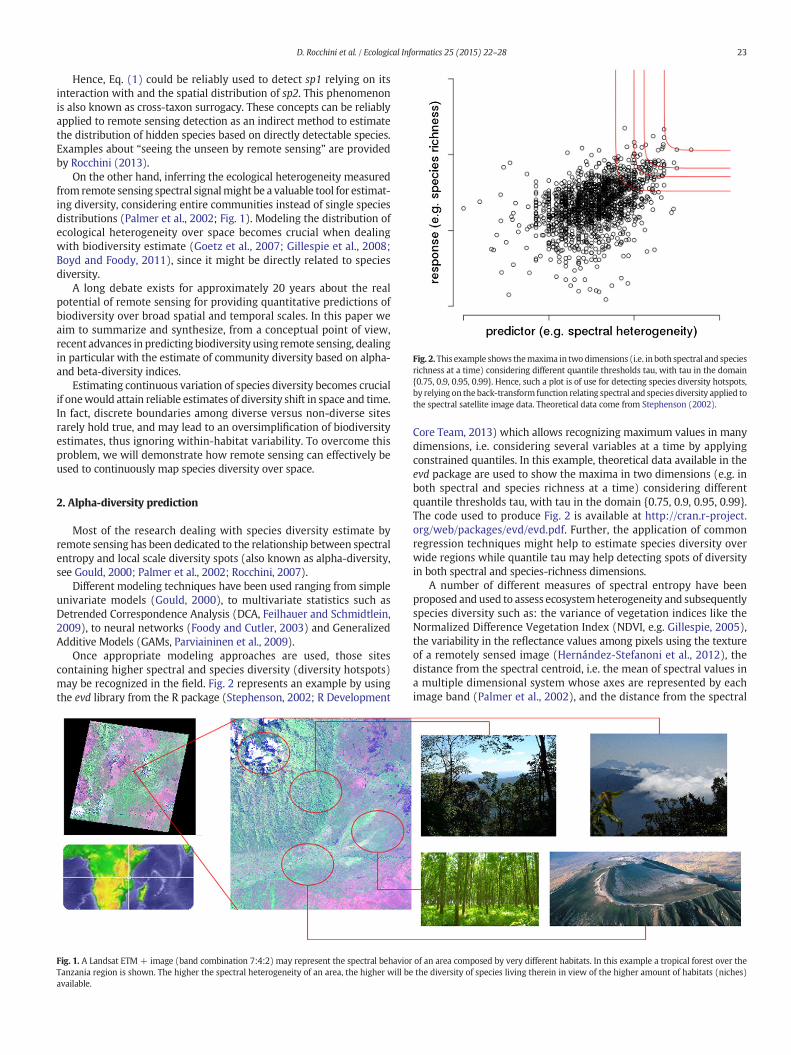
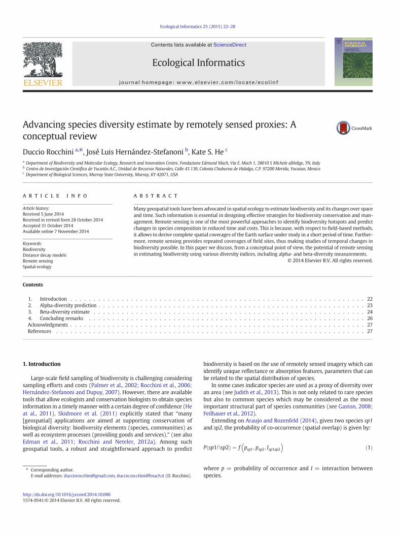
Fig. 2.This example shows themaxima in two dimensions (i.e. in both spectral and speciesrichness at a time) considering different quantile thresholds tau, with tau in the domain{0.75, 0.9, 0.95, 0.99}. Hence, such a plot is of use for detecting species diversity hotspots,by relying on the back-transform function relating spectral and species diversity applied tothe spectral satellite image data. Theoretical data come from Stephenson (2002).

23D. Rocchini et al. / Ecological Informatics 25 (2015) 22–28

Hence, Eq. (1) could be reliably used to detect sp1 relying on itsinteraction with and the spatial distribution of sp2. This phenomenonis also known as cross-taxon surrogacy. These concepts can be reliablyapplied to remote sensing detection as an indirect method to estimatethe distribution of hidden species based on directly detectable species.Examples about “seeing the unseen by remote sensing” are providedby Rocchini (2013).

On the other hand, inferring the ecological heterogeneity measuredfrom remote sensing spectral signalmight be a valuable tool for estimat-ing diversity, considering entire communities instead of single speciesdistributions (Palmer et al., 2002; Fig. 1). Modeling the distribution ofecological heterogeneity over space becomes crucial when dealingwith biodiversity estimate (Goetz et al., 2007; Gillespie et al., 2008;Boyd and Foody, 2011), since it might be directly related to speciesdiversity.

A long debate exists for approximately 20 years about the realpotential of remote sensing for providing quantitative predictions ofbiodiversity over broad spatial and temporal scales. In this paper weaim to summarize and synthesize, from a conceptual point of view,recent advances in predicting biodiversity using remote sensing, dealingin particular with the estimate of community diversity based on alpha-and beta-diversity indices.

Estimating continuous variation of species diversity becomes crucialif onewould attain reliable estimates of diversity shift in space and time.In fact, discrete boundaries among diverse versus non-diverse sitesrarely hold true, and may lead to an oversimplification of biodiversityestimates, thus ignoring within-habitat variability. To overcome thisproblem, we will demonstrate how remote sensing can effectively beused to continuously map species diversity over space.

2. Alpha-diversity prediction

Most of the research dealing with species diversity estimate byremote sensing has been dedicated to the relationship between spectralentropy and local scale diversity spots (also known as alpha-diversity,see Gould, 2000; Palmer et al., 2002; Rocchini, 2007).

Different modeling techniques have been used ranging from simpleunivariate models (Gould, 2000), to multivariate statistics such asDetrended Correspondence Analysis (DCA, Feilhauer and Schmidtlein,2009), to neural networks (Foody and Cutler, 2003) and GeneralizedAdditive Models (GAMs, Parviaininen et al., 2009).

Once appropriate modeling approaches are used, those sitescontaining higher spectral and species diversity (diversity hotspots)may be recognized in the field. Fig. 2 represents an example by usingthe evd library from the R package (Stephenson, 2002; R Development

Fig. 1. A Landsat ETM + image (band combination 7:4:2) may represent the spectral behaviorTanzania region is shown. The higher the spectral heterogeneity of an area, the higher will beavailable.

Core Team, 2013) which allows recognizing maximum values in manydimensions, i.e. considering several variables at a time by applyingconstrained quantiles. In this example, theoretical data available in theevd package are used to show the maxima in two dimensions (e.g. inboth spectral and species richness at a time) considering differentquantile thresholds tau, with tau in the domain {0.75, 0.9, 0.95, 0.99}.The code used to produce Fig. 2 is available at http://cran.r-project.org/web/packages/evd/evd.pdf. Further, the application of commonregression techniques might help to estimate species diversity overwide regions while quantile tau may help detecting spots of diversityin both spectral and species-richness dimensions.

A number of different measures of spectral entropy have beenproposed and used to assess ecosystemheterogeneity and subsequentlyspecies diversity such as: the variance of vegetation indices like theNormalized Difference Vegetation Index (NDVI, e.g. Gillespie, 2005),the variability in the reflectance values among pixels using the textureof a remotely sensed image (Hernández-Stefanoni et al., 2012), thedistance from the spectral centroid, i.e. the mean of spectral values ina multiple dimensional system whose axes are represented by eachimage band (Palmer et al., 2002), and the distance from the spectral

of an area composed by very different habitats. In this example a tropical forest over thethe diversity of species living therein in view of the higher amount of habitats (niches)

24 D. Rocchini et al. / Ecological Informatics 25 (2015) 22–28

centroid in a Principal Component space, i.e. the compacted spectralspace where noise related to band collinearity has been removed(Rocchini, 2007). All such measures have been proven useful in a GISenvironment to predict species richness at local scale; in addition,such models can reach the R2 up to 0.5, which can be considered avalid result since it is based only on spectral variables. Such estimatesare expected to be higher once additional variables representing localclimate conditions, ecosystem fluctuations, disturbance, and topogra-phy are explicitly taken into account in themodel building process. Ad-ditionally, Shannon based information indices have been tested tomeasure spectral heterogeneity with remote sensing data (Rocchiniand Neteler, 2012b) or from land use maps (Ricotta, 2005). However,given the fact that Shannon index is a point measure of species or spec-tral diversity, therefore, the use of generalized entropy for a continuumof diversity measures may be of high value. For example, Rocchini andNeteler (2012b) recently found apparent problems when relying onlyon point descriptors metrics, such as: i) the impossibility to distinguishdifferent ecological situations using one single index of diversity and ii)the impossibility to discern differences in richness or relative abun-dance. For instance, they provide a theoretical example in which areasdiffering in richness or relative abundances of reflectance values(DNs) may show a similar Shannon index value.

Rényi (1970) proposed a generalized entropy Hα ¼ 11−α ln ∑

N

i¼1pα ,

which is extremely flexible and powerful since many popular diversityindices are simply special cases of Hα, e.g.:

Ha ¼ln richnessð Þ for α ¼ 0H

0 ¼ −X

i¼1N p� ln pð Þ for α→1

ln1D

� �for α ¼ 2

8>><>>:

where H′ = Shannon entropy and D = Simpson dominance.While traditional metrics like the Shannon and Simpson entropy

metrics or the Pielou evenness index, supply point descriptions of diver-sity, in Rényi's framework there is a continuum of possible diversitymeasures, which differ in their sensitivity to rare and abundant DNs,becoming increasingly regulated by the commonest DNs when increas-ing the values of α. That is why Rényi's generalized entropy has beenreferred to as a continuum of diversity measures and has been success-fully applied to demonstrate the power of discriminating among land-scapes richness and evenness by a single generalized formula appliedto remote sensing data (Ricotta et al., 2003). Further, Rocchini et al.(2013) applied the method using free and open source code, relyingon the software GRASS GIS (Neteler et al., 2012), to allow reproducibil-ity of the results.

Beside the importance of the correct measure to be used for relatingspectral and species diversity at local scale (alpha-diversity), differentspecies diversity measures can lead to a different power in the results.For example, Oldeland et al. (2010), dealingwith plant species diversityin African savannas, relied on relative abundances of species, as mea-sured by the Shannon index to quantify the difference in the relativeproportion of each species. They demonstrated that accounting forspecies relative abundances improves the capability of detecting localspecies diversity with hyperspectral remotely sensed data, reaching R2

values up to 5 times higher than those achieved by only consideringspecies richness (0.62 and 0.12, respectively). This is mainly due tothe fact that the Shannon index is less affected than species richnessby the presence of rare species, which represent a relatively incidentalset of species of more “dispersed” origin (Ricotta et al., 2008).

Furthermore, recent studies made use of different clustering algo-rithms like support vector machines and multiple clustering models(Baldeck and Asner, 2013; Féret and Asner, 2014) applied to high spatialresolution spectroscopic imagery showing a good capability to mapalpha and beta diversity.

Concerning temporal fluctuations of species diversity, an interestingaspect has been raised by Oindo and Skidmore (2002) who posed theattention to the interannual variability in NDVI in explaining speciesdiversity patterns (considering both vascular plants and mammal spe-cies). The best predictor was found to be the interannual integratedNDVI, including both its average (negative polynomial relationshipwith species richness) and its coefficient of variation (linear relation-ship). From the “temporal” point of view, remote sensing is a valuabletool since it offers the capability of extracting multitemporal univariateor multivariate statistics as predictors instead of relying on single-datepredictors of species diversity. The same holds for intra-annual variabil-ity as demonstrated by He et al. (2009) who foundMarch derived NDVIvariability to be the best predictor over a wide range of NDVI-basedmeasures,mainly because of the phenological changes of the vegetationunder study.

3. Beta-diversity estimate

A study by Tuomisto and Ruokolainen (2006) highlighted how beta-diversity may be “analyzed” or simply “explained” depending on thetarget of the method being used. In most studies addressing beta-diversity (species turnover among sites) and using remotely senseddata, beta-diversity is mainly analyzed with no prediction/explanationoutput. In particular, models have been built to relate species turnoverand spectral turnover to explain the potential relationship and its causesinstead of focusing on the prediction of species turnover over space(Rocchini et al., 2009).

This has been mainly related to spectral distance decay models inwhich species similarity decays once spectral distance d increases,using all pair-wise distances in the square matrix Md below:

Md ¼

d1;1 d1;2 d1;3 ⋯ d1;nd2;1 d2;2 d2;3 ⋯ d2;nd3;1 d3;2 d3;3 ⋯ d3;n⋮ ⋮ ⋮ ⋱ ⋮

dn;1 dn;2 dn;3 ⋯ dn;n

0BBBB@

1CCCCA ð2Þ

or more simply , once N plots are considered, based on an a priori

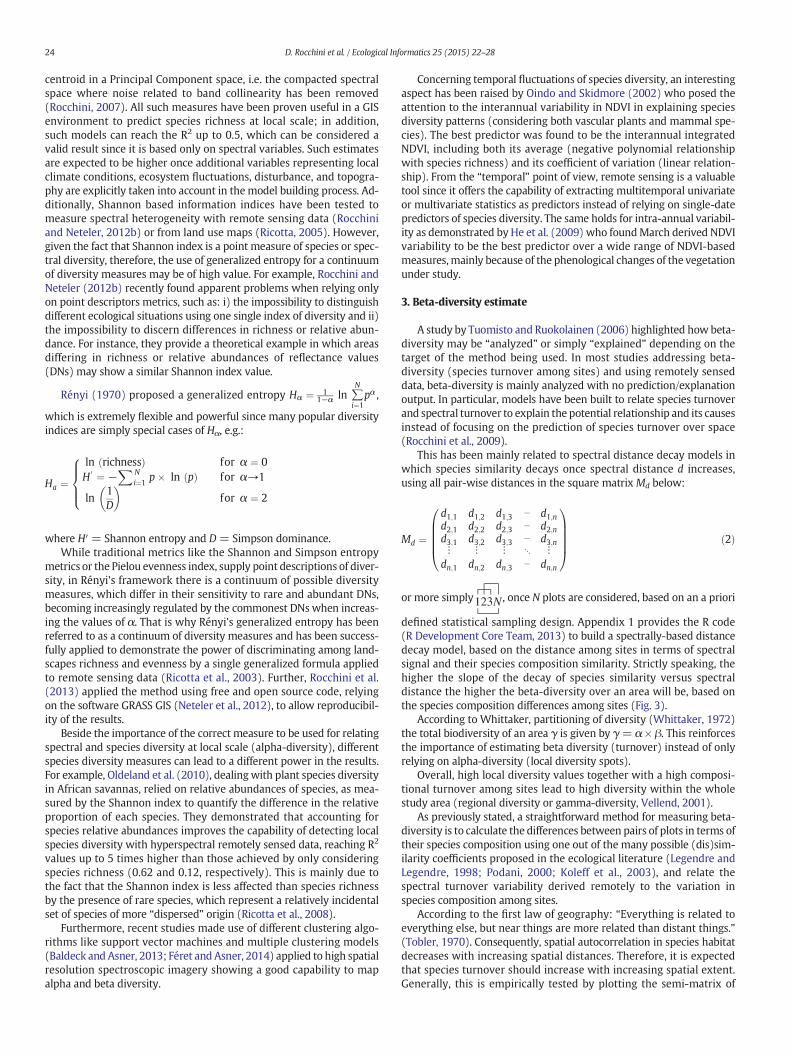
defined statistical sampling design. Appendix 1 provides the R code(R Development Core Team, 2013) to build a spectrally-based distancedecay model, based on the distance among sites in terms of spectralsignal and their species composition similarity. Strictly speaking, thehigher the slope of the decay of species similarity versus spectraldistance the higher the beta-diversity over an area will be, based onthe species composition differences among sites (Fig. 3).

According to Whittaker, partitioning of diversity (Whittaker, 1972)the total biodiversity of an area γ is given by γ= α × β. This reinforcesthe importance of estimating beta diversity (turnover) instead of onlyrelying on alpha-diversity (local diversity spots).

Overall, high local diversity values together with a high composi-tional turnover among sites lead to high diversity within the wholestudy area (regional diversity or gamma-diversity, Vellend, 2001).

As previously stated, a straightforward method for measuring beta-diversity is to calculate the differences between pairs of plots in terms oftheir species composition using one out of the many possible (dis)sim-ilarity coefficients proposed in the ecological literature (Legendre andLegendre, 1998; Podani, 2000; Koleff et al., 2003), and relate thespectral turnover variability derived remotely to the variation inspecies composition among sites.

According to the first law of geography: “Everything is related toeverything else, but near things are more related than distant things.”(Tobler, 1970). Consequently, spatial autocorrelation in species habitatdecreases with increasing spatial distances. Therefore, it is expectedthat species turnover should increase with increasing spatial extent.Generally, this is empirically tested by plotting the semi-matrix of

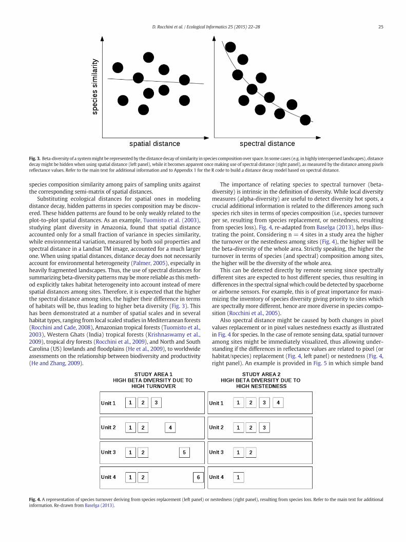
Fig. 3. Beta-diversity of a systemmight be represented by the distance decay of similarity in species composition over space. In some cases (e.g. in highly interspersed landscapes), distancedecay might be hidden when using spatial distance (left panel), while it becomes apparent oncemaking use of spectral distance (right panel), as measured by the distance among pixelsreflectance values. Refer to the main text for additional information and to Appendix 1 for the R code to build a distance decay model based on spectral distance.

25D. Rocchini et al. / Ecological Informatics 25 (2015) 22–28

species composition similarity among pairs of sampling units againstthe corresponding semi-matrix of spatial distances.

Substituting ecological distances for spatial ones in modelingdistance decay, hidden patterns in species composition may be discov-ered. These hidden patterns are found to be only weakly related to theplot-to-plot spatial distances. As an example, Tuomisto et al. (2003),studying plant diversity in Amazonia, found that spatial distanceaccounted only for a small fraction of variance in species similarity,while environmental variation, measured by both soil properties andspectral distance in a Landsat TM image, accounted for a much largerone. When using spatial distances, distance decay does not necessarilyaccount for environmental heterogeneity (Palmer, 2005), especially inheavily fragmented landscapes. Thus, the use of spectral distances forsummarizing beta-diversity patternsmay bemore reliable as thismeth-od explicitly takes habitat heterogeneity into account instead of merespatial distances among sites. Therefore, it is expected that the higherthe spectral distance among sites, the higher their difference in termsof habitats will be, thus leading to higher beta diversity (Fig. 3). Thishas been demonstrated at a number of spatial scales and in severalhabitat types, ranging from local scaled studies inMediterranean forests(Rocchini and Cade, 2008), Amazonian tropical forests (Tuomisto et al.,2003), Western Ghats (India) tropical forests (Krishnaswamy et al.,2009), tropical dry forests (Rocchini et al., 2009), and North and SouthCarolina (US) lowlands and floodplains (He et al., 2009), to worldwideassessments on the relationship between biodiversity and productivity(He and Zhang, 2009).

Fig. 4. A representation of species turnover deriving from species replacement (left panel) orinformation. Re-drawn from Baselga (2013).

The importance of relating species to spectral turnover (beta-diversity) is intrinsic in the definition of diversity. While local diversitymeasures (alpha-diversity) are useful to detect diversity hot spots, acrucial additional information is related to the differences among suchspecies rich sites in terms of species composition (i.e., species turnoverper se, resulting from species replacement, or nestedness, resultingfrom species loss). Fig. 4, re-adapted from Baselga (2013), helps illus-trating the point. Considering n = 4 sites in a study area the higherthe turnover or the nestedness among sites (Fig. 4), the higher will bethe beta-diversity of the whole area. Strictly speaking, the higher theturnover in terms of species (and spectral) composition among sites,the higher will be the diversity of the whole area.

This can be detected directly by remote sensing since spectrallydifferent sites are expected to host different species, thus resulting indifferences in the spectral signalwhich could be detected by spaceborneor airborne sensors. For example, this is of great importance for maxi-mizing the inventory of species diversity giving priority to sites whichare spectrally more different, hence are more diverse in species compo-sition (Rocchini et al., 2005).

Also spectral distance might be caused by both changes in pixelvalues replacement or in pixel values nestedness exactly as illustratedin Fig. 4 for species. In the case of remote sensing data, spatial turnoveramong sites might be immediately visualized, thus allowing under-standing if the differences in reflectance values are related to pixel (orhabitat/species) replacement (Fig. 4, left panel) or nestedness (Fig. 4,right panel). An example is provided in Fig. 5 in which simple band

nestedness (right panel), resulting from species loss. Refer to the main text for additional

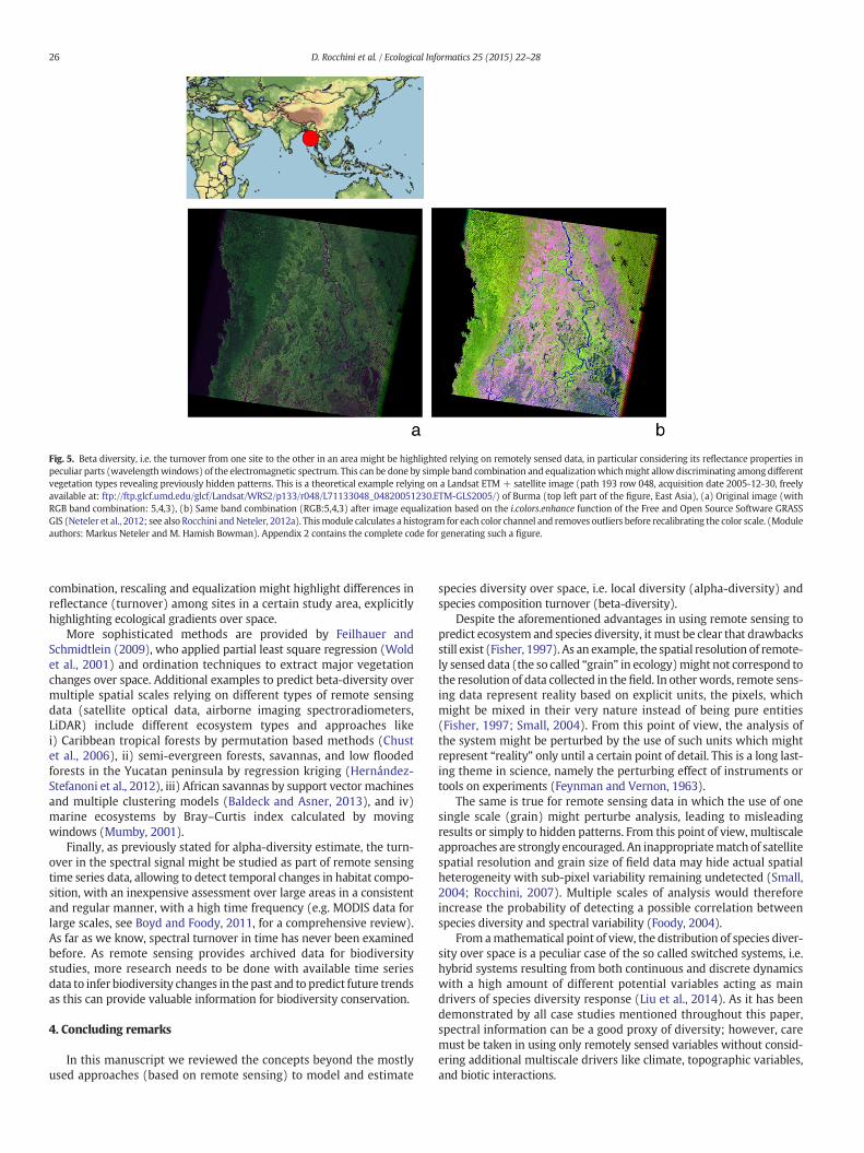
Fig. 5. Beta diversity, i.e. the turnover from one site to the other in an area might be highlighted relying on remotely sensed data, in particular considering its reflectance properties inpeculiar parts (wavelengthwindows) of the electromagnetic spectrum. This can be done by simple band combination and equalizationwhichmight allow discriminating among differentvegetation types revealing previously hidden patterns. This is a theoretical example relying on a Landsat ETM + satellite image (path 193 row 048, acquisition date 2005-12-30, freelyavailable at: ftp://ftp.glcf.umd.edu/glcf/Landsat/WRS2/p133/r048/L71133048_04820051230.ETM-GLS2005/) of Burma (top left part of the figure, East Asia), (a) Original image (withRGB band combination: 5,4,3), (b) Same band combination (RGB:5,4,3) after image equalization based on the i.colors.enhance function of the Free and Open Source Software GRASSGIS (Neteler et al., 2012; see also Rocchini andNeteler, 2012a). Thismodule calculates a histogram for each color channel and removes outliers before recalibrating the color scale. (Moduleauthors: Markus Neteler and M. Hamish Bowman). Appendix 2 contains the complete code for generating such a figure.

26 D. Rocchini et al. / Ecological Informatics 25 (2015) 22–28

combination, rescaling and equalization might highlight differences inreflectance (turnover) among sites in a certain study area, explicitlyhighlighting ecological gradients over space.

More sophisticated methods are provided by Feilhauer andSchmidtlein (2009), who applied partial least square regression (Woldet al., 2001) and ordination techniques to extract major vegetationchanges over space. Additional examples to predict beta-diversity overmultiple spatial scales relying on different types of remote sensingdata (satellite optical data, airborne imaging spectroradiometers,LiDAR) include different ecosystem types and approaches likei) Caribbean tropical forests by permutation based methods (Chustet al., 2006), ii) semi-evergreen forests, savannas, and low floodedforests in the Yucatan peninsula by regression kriging (Hernández-Stefanoni et al., 2012), iii) African savannas by support vector machinesand multiple clustering models (Baldeck and Asner, 2013), and iv)marine ecosystems by Bray–Curtis index calculated by movingwindows (Mumby, 2001).

Finally, as previously stated for alpha-diversity estimate, the turn-over in the spectral signal might be studied as part of remote sensingtime series data, allowing to detect temporal changes in habitat compo-sition, with an inexpensive assessment over large areas in a consistentand regular manner, with a high time frequency (e.g. MODIS data forlarge scales, see Boyd and Foody, 2011, for a comprehensive review).As far as we know, spectral turnover in time has never been examinedbefore. As remote sensing provides archived data for biodiversitystudies, more research needs to be done with available time seriesdata to infer biodiversity changes in the past and to predict future trendsas this can provide valuable information for biodiversity conservation.

4. Concluding remarks

In this manuscript we reviewed the concepts beyond the mostlyused approaches (based on remote sensing) to model and estimate

species diversity over space, i.e. local diversity (alpha-diversity) andspecies composition turnover (beta-diversity).

Despite the aforementioned advantages in using remote sensing topredict ecosystem and species diversity, it must be clear that drawbacksstill exist (Fisher, 1997). As an example, the spatial resolution of remote-ly sensed data (the so called “grain” in ecology)might not correspond tothe resolution of data collected in the field. In other words, remote sens-ing data represent reality based on explicit units, the pixels, whichmight be mixed in their very nature instead of being pure entities(Fisher, 1997; Small, 2004). From this point of view, the analysis ofthe system might be perturbed by the use of such units which mightrepresent “reality” only until a certain point of detail. This is a long last-ing theme in science, namely the perturbing effect of instruments ortools on experiments (Feynman and Vernon, 1963).

The same is true for remote sensing data in which the use of onesingle scale (grain) might perturbe analysis, leading to misleadingresults or simply to hidden patterns. From this point of view, multiscaleapproaches are strongly encouraged. An inappropriatematch of satellitespatial resolution and grain size of field data may hide actual spatialheterogeneity with sub-pixel variability remaining undetected (Small,2004; Rocchini, 2007). Multiple scales of analysis would thereforeincrease the probability of detecting a possible correlation betweenspecies diversity and spectral variability (Foody, 2004).

From amathematical point of view, the distribution of species diver-sity over space is a peculiar case of the so called switched systems, i.e.hybrid systems resulting from both continuous and discrete dynamicswith a high amount of different potential variables acting as maindrivers of species diversity response (Liu et al., 2014). As it has beendemonstrated by all case studies mentioned throughout this paper,spectral information can be a good proxy of diversity; however, caremust be taken in using only remotely sensed variables without consid-ering additional multiscale drivers like climate, topographic variables,and biotic interactions.

27D. Rocchini et al. / Ecological Informatics 25 (2015) 22–28

Moreover, the uncertainty related to remote sensing input data andto the models being used for species diversity prediction should be ex-plicitly taken into account, by mapping uncertainty over space, relyingon the so called maps of ignorance (Boggs, 1949) representing thebias or the uncertainty, alongside predictive maps (Rocchini et al.,2011). Uncertainty can derive from a number of input data sources,such as the definition or identification of certain species, or the afore-mentioned scale mismatch between remote sensing and species data,as well as location-based errors. In addition, maps derived from theoverlap of different thematic layers, may lead to uncertainty related tothe modeling procedure being adopted (Arbia et al., 1998). Hence, thespatial distribution of uncertainty should be explicitly shown on mapsto avoid ignoring overall accuracy or model errors. Quoting Swansonet al. (2013) “including such estimates alongside mean projectionsgives a map of ignorance as called for by Rocchini et al. (2011),highlighting areas where knowledge is lacking and could be improvedwith additional sampling effort or the inclusion of additionalcovariates.”

In this manuscript we did not take into account zero inflateddatasets which in some cases arise from particularly extreme environ-ments where no species are recorded. We refer to Feng and Dean(2012) for a complete dissertation about the possibility of analyzingzero-inflated datasets based on the so called “spatial factor models”.As far as we know no applications have been done in this sense usingremote sensing data, while zero-inflated sets have been demonstratedto be the rule rather than the exception (see Rocchini, 2007). Thisrepresents one of the future challenges in spatial ecology focusing onremote sensing based prediction of biodiversity.

Supplementary data to this article can be found online at http://dx.doi.org/10.1016/j.ecoinf.2014.10.006.

Acknowledgments

We are grateful to the handling Editor G.M. Foody and to two anon-ymous reviewers for precious insights on a previous version of themanuscript. DR is supported by the EU BON (Building the EuropeanBiodiversity Observation Network) project, funded by the EuropeanUnion under the 7th Framework programme, Contract No. 308454and by the ERANET BioDiversa FP7 project DIARS, funded by theEuropean Union.

References

Araujo, M.B., Rozenfeld, A., 2014. The geographic scaling of biotic interactions. Ecography5, 406–415.

Arbia, G., Griffith, D.A., Haining, R.P., 1998. Error propagation modelling in raster GIS:overlay operations. Int. J. Geogr. Inf. Sci. 12, 145–167.

Baldeck, C.A., Asner, G.P., 2013. Estimating vegetation beta diversity from airborneimaging spectroscopy and unsupervised clustering. Remote Sens. 5, 2057–2071.

Baselga, A., 2013. Multiple site dissimilarity quantifies compositional heterogeneityamong several sites, while average pairwise dissimilarity may be misleading.Ecography 36, 124–128.

Boggs, S.W., 1949. An atlas of ignorance: a needed stimulus to honest thinking and hardwork. Proc. Am. Philos. Soc. 93, 253–258.

Boyd, D.S., Foody, G.M., 2011. An overview of recent remote sensing and GIS basedresearch in ecological informatics. Ecol. Inform. 6, 25–36.

Chust, G., Chave, J., Condit, R., Anguilar, S., Lao, S., Prez, R., 2006. Determinants and spatialmodeling of tree β-diversity in a tropical forest landscape in Panama. J. Veg. Sci. 17,83–92.

Edman, T., Angelstam, P., Mikusinski, G., Roberge, J.-M., Sikora, A., 2011. Spatial planningfor biodiversity conservation: assessment of forest landscapes conservation valueusing umbrella species requirements in Poland. Landsc. Urban Plan. 102, 16–23.

Feilhauer, H., Schmidtlein, S., 2009. Mapping continuous fields of forest alpha and betadiversity. Appl. Veg. Sci. 12, 429–439.

Feilhauer, H., He, K.S., Rocchini, D., 2012. Modeling species distribution using niche-basedproxies derived from composite bioclimatic variables and MODIS NDVI. Remote Sens.4, 2057–2075.

Feng, C.X., Dean, C.B., 2012. Joint analysis of multivariate spatial count and zero-heavycount outcomes using common spatial factor models. Environmetrics 23, 493–508.

Féret, J.-B., Asner, G.P., 2014. Mapping tropical forest canopy diversity using high-fidelityimaging spectroscopy. Ecol. Appl. 24, 1289–1296.

Feynman, R.P., Vernon Jr., F.L., 1963. The theory of a general quantum system interactingwith a linear dissipative system. Ann. Phys. 34, 118–173.

Fisher, P.F., 1997. The pixel: a snare and a delusion. Int. J. Remote Sens. 18, 679–685.Foody, G.M., 2004. Spatial nonstationarity and scale-dependency in the relationship

between species richness and environmental determinants for the sub-Saharanendemic avifauna. Glob. Ecol. Biogeogr. 13, 315–320.

Foody, G.M., Cutler, M.E.J., 2003. Tree biodiversity in protected and logged Borneantropical rain forests and its measurement by satellite remote sensing. J. Biogeogr.30, 1053–1066.

Gaston, K.J., 2008. Biodiversity and extinction: the importance of being common. Prog.Phys. Geogr. 32, 73–79.

Gillespie, T.W., 2005. Predicting woody-plant species richness in tropical dry forests: acase study from South Florida, USA. Ecol. Appl. 15, 27–37.

Gillespie, T.W., Foody, G.M., Rocchini, D., Giorgi, A.P., Saatchi, S., 2008. Measuring andmodelling biodiversity from space. Prog. Phys. Geogr. 32, 203–221.

Goetz, S., Steinberg, D., Dubayah, R., Blair, B., 2007. Laser remote sensing of canopy habitatheterogeneity as a predictor of bird species richness in an eastern temperate forest,USA. Remote Sens. Environ. 108, 254–263.

Gould, W., 2000. Remote sensing of vegetation, plant species richness, and regionalbiodiversity hot spots. Ecol. Appl. 10, 1861–1870.

He, K.S., Zhang, J., 2009. Testing the correlation between beta diversity and differences inproductivity among global ecoregions, biomes, and biogeographical realms. Ecol.Inform. 4, 93–98.

He, K.S., Zhang, J., Zhang, Q., 2009. Linking variability in species composition and MODISNDVI based on beta diversity measurements. Acta Oecol. 35, 14–21.

He, K.S., Rocchini, D., Neteler, M., Nagendra, H., 2011. Benefits of hyperspectral remotesensing for tracking plant invasions. Divers. Distrib. 17, 381–392.

Hernández-Stefanoni, J., Dupuy, J., 2007. Mapping species density of trees, shrubs andvines in a tropical forest, using field measurements, satellite multispectral imageryand spatial interpolation. Biodivers. Conserv. 16, 3817–3833.

Hernández-Stefanoni, J.L., Gallardo-Cruz, J.A., Meave, J.A., Rocchini, D., Bello-Pineda, J.,López-Martínez, J.O., 2012. Modeling alpha- and beta-diversity in a tropical forestfrom remotely sensed and spatial data. Int. J. Appl. Earth Obs. Geoinformation 19,359–368.

Judith, C., Schneider, J.V., Schmidt, M., Ortega, R., Gaviria, J., Zizka, G., 2013. Using high-resolution remote sensing data for habitat suitability models of Bromeliaceae in thecity of Merida, Venezuela. Landsc. Urban Plan. 120, 107–118.

Koleff, P., Gaston, K.J., Lennon, J.J., 2003. Measuring beta diversity for presence–absencedata. J. Anim. Ecol. 72, 367–382.

Krishnaswamy, J., Bawa, K.S., Ganeshaiah, K.N., Kiran, M.C., 2009. Quantifyingand mapping biodiversity and ecosystem services: utility of a multi-seasonNDVI based Mahalanobis distance surrogate. Remote Sens. Environ. 113,857–867.

Legendre, P., Legendre, L., 1998. Numerical Ecology. Elsevier, Amsterdam.Liu, X., Zhong, S., Ding, X., 2014. A Razumikhin approach to exponential admissi-

bility of switched descriptor delayed systems. Appl. Math. Model. 38,1647–1659.

Mumby, P.J., 2001. Beta and habitat diversity in marine systems: a new approach tomeasurement, scaling and interpretation. Oecologia 128, 274–280.

Neteler, M., Bowman, M.H., Landa, M., Metz, M., 2012. GRASS GIS: a multi-purpose OpenSource GIS. Environ. Model. Softw. 31, 124–130.

Oindo, B.O., Skidmore, A.K., 2002. Interannual variability of NDVI and species richness inKenya. Int. J. Remote Sens. 23, 285–298.

Oldeland, J., Wesuls, D., Rocchini, D., Schmidt, M., Jrgens, N., 2010. Does using speciesabundance data improve estimates of species diversity from remotely sensed spectralheterogeneity? Ecol. Indic. 10, 390–396.

Palmer, M.W., 2005. Distance decay in an old-growth neotropical forest. J. Veg. Sci. 16,161–166.

Palmer, M.W., Earls, P., Hoagland, B.W., White, P.S., Wohlgemuth, T., 2002. Quantitativetools for perfecting species lists. Environmetrics 13, 121–137.

Parviainen, M., Luoto, M., Heikkinen, R.K., 2009. The role of local and landscape levelmeasures of greenness in modelling boreal plant species richness. Ecol. Model. 220,2690–2701.

Podani, J., 2000. Introduction to the Exploration of Multivariate Biological Data. Backhuys,Leiden, NL.

R Development Core Team, 2013. R: A Language and Environment for Statistical Computing.the R Foundation for Statistical Computing, Vienna, Austria.

Rényi, A., 1970. Probability Theory. North Holland Publishing Company, Amsterdam.Ricotta, C., 2005. On possible measures for evaluating the degree of uncertainty of fuzzy

thematic maps. Int. J. Remote Sens. 26, 5573–5583.Ricotta, C., Corona, P., Marchetti, M., Chirici, G., Innamorati, S., 2003. LaDy: software for

assessing local landscape diversity profiles of raster land covermaps using geographicwindows. Environ. Model Softw. 18, 373–378.

Ricotta, C., Godefroid, S., Celesti-Grapow, L., 2008. Common species have lower taxonomicdiversity: evidence from the urban floras of Brussels and Rome. Divers. Distrib. 14,530–537.

Rocchini, D., 2007. Effects of spatial and spectral resolution in estimating ecosystemα-diversity by satellite imagery. Remote Sens. Environ. 111, 423–434.

Rocchini, D., 2013. Seeing the unseen by remote sensing: satellite imagery applied tospecies distribution modelling. J. Veg. Sci. 24, 209–210.

Rocchini, D., Cade, B.S., 2008. Quantile regression applied to spectral distance decay. IEEEGeosci. Remote Sens. Lett. 5, 640–643.

Rocchini, D., Neteler, M., 2012a. Let the four freedoms paradigm apply to ecology. TrendsEcol. Evol. 27, 310–311.

Rocchini, D., Neteler, M., 2012b. Spectral rank-abundance for measuring landscapediversity. Int. J. Remote Sens. 33, 4458–4470.

28 D. Rocchini et al. / Ecological Informatics 25 (2015) 22–28

Rocchini, D., Andreini Butini, S., Chiarucci, A., 2005. Maximizing plant species inventoryefficiency by means of remotely sensed spectral distances. Glob. Ecol. Biogeogr. 14,431–437.

Rocchini, D., Perry, G.L.W., Salerno, M., Maccherini, S., Chiarucci, A., 2006. Landscapechange and the dynamics of open formations in a natural reserve. Landsc. UrbanPlan. 77, 167–177.

Rocchini, D., Nagendra, H., Ghate, R., Cade, B.S., 2009. Spectral distance decay: assessingspecies beta-diversity by quantile regression. Photogramm. Eng. Remote. Sens. 75,1225–1230.

Rocchini, D., Hortal, J., Lengyel, S., Lobo, J.M., Jiménez-Valverde, A., Ricotta, C., Bacaro, G.,Chiarucci, A., 2011. Accounting for uncertainty when mapping species distributions:the need for maps of ignorance. Prog. Phys. Geogr. 35, 211–226.

Rocchini, D., Delucchi, L., Bacaro, G., Cavallini, P., Feilhauer, H., Foody, G.M., He, K.S.,Nagendra, H., Porta, C., Ricotta, C., Schmidtlein, S., Spano, L.D., Wegmann, M.,Neteler, M., 2013. Calculating landscape diversity with information-theory basedindices: a GRASS GIS solution. Ecol. Inform 17, 82–93.

Skidmore, A., Franklin, J., Dawson, T.P., Pilesjo, P., 2011. Geospatial tools address emergingissues in spatial ecology: a review and commentary on the Special Issue. Int. J. Geogr.Inf. Sci. 25, 337–365.

Small, C., 2004. The Landsat ETM + spectral mixing space. Remote Sens. Environ. 93,1–17.

Stephenson, A.G., 2002. evd: Extreme Value Distributions. R News, 2, 2.Swanson, A.K., Dobrowski, S.Z., Finley, A.O., Thorne, J.H., Schwartz, M.K., 2013. Spatial

regression methods capture prediction uncertainty in species distribution modelprojections through time. Glob. Ecol. Biogeogr. 22, 242–251.

Tobler, W., 1970. A computer movie simulating urban growth in the Detroit region. Econ.Geogr. 46, 234–240.

Tuomisto, H., Ruokolainen, K., 2006. Analyzing or explaining beta diversity? Understandingthe targets of different methods of analysis. Ecology 87, 2697–2708.

Tuomisto, H., Poulsen, A.D., Ruokolainen, K., Moran, R.C., Quintana, C., Celi, J., Caas, G.,2003. Linking floristic patterns with soil heterogeneity and satellite imagery inEcuadorian Amazonia. Ecol. Appl. 13, 352–371.

Vellend, M., 2001. Do commonly used indices of diversity measure species turnover? J.Veg. Sci. 12, 545–552.

Whittaker, R.H., 1972. Evolution and measurement of species diversity. Taxon 21,213–251.

Wold, S., Sjöström, M., Eriksson, L., 2001. PLS-regression: a basic tool of chemometrics.Chemometr. Intell. Lab. Syst. 58, 109130.