Aeroacoustic Optimization of Wind Turbine Blades

Simão Santos Rodrigues

Thesis to obtain the Master of Science Degree in

Aerospace Engineering

Examination Committee

Chairperson: Professor Fernando José Parracho Lau

Supervisor: Doctor André Calado Marta

Members of the Committee: Professor João Manuel Gonçalves de Sousa Oliveira

November 2012

ii

“You have brains in your head. You have feet in your shoes.

You can steer yourself

any direction you choose.

You’re on your own. And you know what you know.

And YOU are the one who’ll decide where to go...”

Dr. Seuss, Oh, the Places You’ll Go!

iii

iv

Acknowledgments

I would like to thank my thesis supervisor Dr. Andre Calado Marta for all his teachings and guidance

throughout the development of this thesis. I would also like to leave a thank you to my family for supporting

me financially and emotionally through my studies and to my friends and colleagues, with whom I shared

this journey of my life.

v

vi

Resumo

A producao eolica tem vindo a aumentar, com cada vez mais areas a serem usadas como quintas eolicas

e as turbinas cada vez maiores. Este desenvolvimento levou ao aumento da percepcao dos efeitos das

turbinas eolicas no ambiente e na saude publica. Muita pesquisa tem sido feita no sentido de prever

e reduzir o ruıdo por elas produzido. Neste trabalho, um modelo baseado na teoria dos elementos

de pas-momento linear e utilizado para prever a performance aerodinamica de uma turbina eolica e e

acoplado a um modelo aeroacustico empırico, baseado nos trabalhos de Brooks et al (1989) e Amiet

(1975), que utiliza codigo XFOIL na computacao dos parametros da camada limite. O codigo foi validado

com dados experimentais das turbinas NREL Phase II e AOC 15/50 e posteriormente utilizado no modulo

de optimizacao pyOpt, com o algoritmo genetico NSGA-II. A geometria da pa foi parametrizada utilizando

curvas NURBS para os perfis 2D e curvas de Bezier para a distribuicao da corda e torcao ao longo da

pa. Foram efectuadas varias optimizacoes nas duas turbinas, tanto uni- como multi-objectivo, com um

numero de variaveis de design que chegou aos 62. As solucoes optimas sao indicadas nas frentes de

Pareto obtidas e as suas geometrias discutidas em detalhe. Estas solucoes variam desde um aumento

de 139.4 % da energia produzida anualmente ate uma reducao dos nıveis de ruıdo em 10.7 %. Foi

demonstrado que uma reducao significativa no nıvel de ruıdo pode ser obtida, a custa de uma ligeira

penalidade aerodinamica.

Palavras-chave: Algoritmos geneticos, NURBS, Optimizacao multidisciplinar, Optimizacao

multi-objectivo

vii

viii

Abstract

Power production from wind energy has been increasing for the past few decades, with more areas

being used as wind farms and larger wind turbines being built. With this development, awareness of the

impact of wind energy on the environment and on human health as also increased. Much research has

been done to predict and reduce the noise generated by wind turbines. In this work, a blade element

momentum theory model is used to predict the aerodynamic performance of a wind turbine, coupled

to an empirical aeroacoustic noise model based on the works of Brooks et al (1989) and Amiet (1975),

and using the XFOIL panel code for the boundary layer computations. The aeroacoustic prediction code

developed was validated against measurement data of the NREL Phase II and AOC 15/50 wind turbines

and used in the optimization framework pyOpt, using the genetic algorithm NSGA-II. The geometry of

the blade was parameterized using NURBS curves for the cross sectional airfoil shapes and Bezier

curves for the twist and chord distributions. Various optimizations were performed in blades of the

two previous turbines, both single- and multi-objective, totaling up to 62 design variables. The optimal

solutions are indicated in the obtained Pareto fronts and their geometries are discussed in detail. These

solutions ranged from an increase in annual energy production of 139.9% to a reduction in noise levels of

10.7%. It was demonstrated that significant noise reduction could be obtained at an expense of a minor

aerodynamic penalty.

Keywords: Genetic algorithms, NURBS, Multi-disciplinary design optimization, Multi-objective

optimization

ix

x

Contents

Acknowledgments . . . . . . . . . . . . . . . . . . . . . . . . . . . . . . . . . . . . . . . . . . . v

Resumo . . . . . . . . . . . . . . . . . . . . . . . . . . . . . . . . . . . . . . . . . . . . . . . . . vii

Abstract . . . . . . . . . . . . . . . . . . . . . . . . . . . . . . . . . . . . . . . . . . . . . . . . . ix

List of Tables . . . . . . . . . . . . . . . . . . . . . . . . . . . . . . . . . . . . . . . . . . . . . . xv

List of Figures . . . . . . . . . . . . . . . . . . . . . . . . . . . . . . . . . . . . . . . . . . . . . xix

Nomenclature . . . . . . . . . . . . . . . . . . . . . . . . . . . . . . . . . . . . . . . . . . . . . . xxii

1 Introduction 1

1.1 Wind Energy Worldwide . . . . . . . . . . . . . . . . . . . . . . . . . . . . . . . . . . . . . 1

1.2 Environmental Impact of Wind Energy . . . . . . . . . . . . . . . . . . . . . . . . . . . . . 3

1.3 Legislation on WT Noise . . . . . . . . . . . . . . . . . . . . . . . . . . . . . . . . . . . . . 3

1.4 State of The Art . . . . . . . . . . . . . . . . . . . . . . . . . . . . . . . . . . . . . . . . . . 4

1.5 Report Overview . . . . . . . . . . . . . . . . . . . . . . . . . . . . . . . . . . . . . . . . . 5

2 Wind Turbine Aerodynamics 7

2.1 Actuator Disk Concept . . . . . . . . . . . . . . . . . . . . . . . . . . . . . . . . . . . . . . 7

2.2 Blade Element Momentum Theory . . . . . . . . . . . . . . . . . . . . . . . . . . . . . . . 8

2.2.1 Corrections to BEM theory . . . . . . . . . . . . . . . . . . . . . . . . . . . . . . . 10

2.2.2 Iteration Procedure . . . . . . . . . . . . . . . . . . . . . . . . . . . . . . . . . . . . 12

2.3 Annual Energy Production . . . . . . . . . . . . . . . . . . . . . . . . . . . . . . . . . . . . 12

2.4 Airfoil Aerodynamic Data . . . . . . . . . . . . . . . . . . . . . . . . . . . . . . . . . . . . . 13

2.4.1 3D Stall-Delay Correction . . . . . . . . . . . . . . . . . . . . . . . . . . . . . . . . 13

2.4.2 Polar Extrapolation . . . . . . . . . . . . . . . . . . . . . . . . . . . . . . . . . . . . 14

3 Noise from Wind Turbines 17

3.1 Principles of Acoustics . . . . . . . . . . . . . . . . . . . . . . . . . . . . . . . . . . . . . . 17

3.1.1 Sound Pressure and Power Levels . . . . . . . . . . . . . . . . . . . . . . . . . . . 17

3.1.2 Sound Frequency Spectrum . . . . . . . . . . . . . . . . . . . . . . . . . . . . . . . 18

3.2 Noise Mechanisms in Wind Turbines . . . . . . . . . . . . . . . . . . . . . . . . . . . . . . 19

3.2.1 Mechanical Noise . . . . . . . . . . . . . . . . . . . . . . . . . . . . . . . . . . . . 19

3.2.2 Aerodynamic Noise . . . . . . . . . . . . . . . . . . . . . . . . . . . . . . . . . . . 20

3.3 Noise Prediction Model . . . . . . . . . . . . . . . . . . . . . . . . . . . . . . . . . . . . . 23

xi

3.3.1 Prediction Model for Inflow Turbulence Noise . . . . . . . . . . . . . . . . . . . . . 24

3.3.2 Prediction Model for Turbulent Boundary Layer - Trailing Edge Noise . . . . . . . . 26

3.3.3 Prediction Model for the Laminar Boundary Layer - Vortex Shedding Noise . . . . 27

3.3.4 Prediction Model for Trailing Edge Bluntness Vortex Shedding Noise . . . . . . . . 28

3.3.5 Prediction Model for Tip Vortex Formation Noise . . . . . . . . . . . . . . . . . . . 29

3.3.6 Sound Directivity . . . . . . . . . . . . . . . . . . . . . . . . . . . . . . . . . . . . . 29

3.3.7 Boundary-Layer Calculation . . . . . . . . . . . . . . . . . . . . . . . . . . . . . . . 30

4 Blade Geometry and Parameterization 33

4.1 Twist and Chord distribution . . . . . . . . . . . . . . . . . . . . . . . . . . . . . . . . . . . 33

4.2 Airfoil Shape Distribution . . . . . . . . . . . . . . . . . . . . . . . . . . . . . . . . . . . . . 33

5 Wind Turbine Noise Prediction Code 39

5.1 Code Structure . . . . . . . . . . . . . . . . . . . . . . . . . . . . . . . . . . . . . . . . . . 39

5.2 Code Inputs and Output . . . . . . . . . . . . . . . . . . . . . . . . . . . . . . . . . . . . . 39

5.3 Code Validation . . . . . . . . . . . . . . . . . . . . . . . . . . . . . . . . . . . . . . . . . . 42

5.3.1 2D Airfoil Noise Prediction Validation . . . . . . . . . . . . . . . . . . . . . . . . . . 43

5.3.2 BEM Code Validation . . . . . . . . . . . . . . . . . . . . . . . . . . . . . . . . . . 44

5.3.3 WT Noise Code Validation . . . . . . . . . . . . . . . . . . . . . . . . . . . . . . . . 46

6 Optimization Framework 49

6.1 Numerical Optimization Methods . . . . . . . . . . . . . . . . . . . . . . . . . . . . . . . . 49

6.1.1 Gradient-Based Algorithms . . . . . . . . . . . . . . . . . . . . . . . . . . . . . . . 50

6.1.2 Genetic Algorithms . . . . . . . . . . . . . . . . . . . . . . . . . . . . . . . . . . . . 51

6.2 Framework Description . . . . . . . . . . . . . . . . . . . . . . . . . . . . . . . . . . . . . 51

7 Optimization Results 55

7.1 Optimization of NREL Phase II Turbine Blade . . . . . . . . . . . . . . . . . . . . . . . . . 56

7.1.1 Chord and Twist Optimization . . . . . . . . . . . . . . . . . . . . . . . . . . . . . . 57

7.1.2 Airfoil Shape Optimization . . . . . . . . . . . . . . . . . . . . . . . . . . . . . . . . 60

7.1.3 Chord, Twist and Airfoil Shape Optimization . . . . . . . . . . . . . . . . . . . . . . 65

7.1.4 Summary of the Results . . . . . . . . . . . . . . . . . . . . . . . . . . . . . . . . . 69

7.2 Optimization on the AOC 15/50 Turbine Blade . . . . . . . . . . . . . . . . . . . . . . . . . 70

8 Conclusions 79

8.1 Achievements . . . . . . . . . . . . . . . . . . . . . . . . . . . . . . . . . . . . . . . . . . . 79

8.2 Future Work . . . . . . . . . . . . . . . . . . . . . . . . . . . . . . . . . . . . . . . . . . . . 80

A Coordinate Systems 81

xii

B Noise Model Equations and Functions 83

B.1 TBL-TE . . . . . . . . . . . . . . . . . . . . . . . . . . . . . . . . . . . . . . . . . . . . . . 83

B.2 LBL-VS . . . . . . . . . . . . . . . . . . . . . . . . . . . . . . . . . . . . . . . . . . . . . . 85

B.3 TEB-VS . . . . . . . . . . . . . . . . . . . . . . . . . . . . . . . . . . . . . . . . . . . . . . 86

C Sample Input Files 87

C.1 Rotor Definition File . . . . . . . . . . . . . . . . . . . . . . . . . . . . . . . . . . . . . . . 87

C.2 Rotor Analysis File . . . . . . . . . . . . . . . . . . . . . . . . . . . . . . . . . . . . . . . . 87

D Sample Optimization Script 89

Bibliography 100

xiii

xiv

List of Tables

1.1 Top 10 leading countries in wind energy production. . . . . . . . . . . . . . . . . . . . . . 2

1.2 Noise limits of sound pressure level according to the Portuguese legislation. . . . . . . . . 3

1.3 Noise limits of equivalent sound pressure levels Leq (dB(A)) in some European countries. 4

3.1 Typical roughness lengths associated with different terrain types. . . . . . . . . . . . . . . 26

4.1 Comparison between various airfoil parameterization methods. . . . . . . . . . . . . . . . 35

5.1 Listing of some of the features of the Section class. . . . . . . . . . . . . . . . . . . . . . 40

5.2 List of some of the features of the Blade class. . . . . . . . . . . . . . . . . . . . . . . . . 40

5.3 Listing of some of the features of the Rotor class. . . . . . . . . . . . . . . . . . . . . . . . 40

5.4 Listing of some of the features of the Polar class. . . . . . . . . . . . . . . . . . . . . . . . 41

5.5 Listing of some of the features of the BLayer class. . . . . . . . . . . . . . . . . . . . . . . 41

5.6 Listing of some of the features of the Analysis class. . . . . . . . . . . . . . . . . . . . . 41

5.7 Parameters of the NACA 0012 noise prediction validation. . . . . . . . . . . . . . . . . . . 43

5.8 NREL Phase II wind turbine characteristics. . . . . . . . . . . . . . . . . . . . . . . . . . . 44

5.9 AOC 15/50 wind turbine characteristics. . . . . . . . . . . . . . . . . . . . . . . . . . . . . 47

7.1 Properties of the air used in the optimizations. . . . . . . . . . . . . . . . . . . . . . . . . . 55

7.2 NREL Phase II optimization cases summary. . . . . . . . . . . . . . . . . . . . . . . . . . 56

7.3 Initial OASPL and AEP values of the NREL Phase II wind turbine. . . . . . . . . . . . . . 56

7.4 Summary of AEP and OASPL values in case 1. . . . . . . . . . . . . . . . . . . . . . . . . 58

7.5 Summary of AEP and OASPL values in case 2. . . . . . . . . . . . . . . . . . . . . . . . . 59

7.6 Summary of AEP and OASPL values in case 3. . . . . . . . . . . . . . . . . . . . . . . . . 61

7.7 Summary of AEP and OASPL values in case 4. . . . . . . . . . . . . . . . . . . . . . . . . 63

7.8 Summary of AEP and OASPL values in case 5. . . . . . . . . . . . . . . . . . . . . . . . . 66

7.9 Summary of the optimization cases performed on the NREL Phase II wind turbine blade. 70

7.10 Initial OASPL and AEP values of the AOC 15/50 wind turbine. . . . . . . . . . . . . . . . . 71

7.11 Summary of AEP and OASPL values in AOC 15/50 optimization case. . . . . . . . . . . . 73

xv

xvi

List of Figures

1.1 Wind energy market forecast of the 2012-2016 period. . . . . . . . . . . . . . . . . . . . . 2

2.1 Actuator disk. . . . . . . . . . . . . . . . . . . . . . . . . . . . . . . . . . . . . . . . . . . . 8

2.2 Velocities at the rotor plane. . . . . . . . . . . . . . . . . . . . . . . . . . . . . . . . . . . . 9

2.3 Glauert correction for tip loss factor F = 1.0. . . . . . . . . . . . . . . . . . . . . . . . . . . 11

2.4 Weibull distribution curve and power curve for a generic wind turbine. . . . . . . . . . . . 13

2.5 Lift and drag coefficients of the S809 airfoil before and after 3D stall delay correction. . . . 14

2.6 Original and extrapolated S809 airfoil data for two different blade aspect ratios. . . . . . . 15

3.1 Sound pressure level examples. . . . . . . . . . . . . . . . . . . . . . . . . . . . . . . . . 18

3.2 A-, B-, C- and D-weightings. . . . . . . . . . . . . . . . . . . . . . . . . . . . . . . . . . . . 19

3.3 Wind turbine noise mechanisms. . . . . . . . . . . . . . . . . . . . . . . . . . . . . . . . . 20

3.4 Representation of the TBL-TE noise mechanism. . . . . . . . . . . . . . . . . . . . . . . . 22

3.5 Representation of the separation-stall noise mechanism. . . . . . . . . . . . . . . . . . . . 22

3.6 Representation of the TEB-VS noise mechanism. . . . . . . . . . . . . . . . . . . . . . . . 23

3.7 Representation of the LBL-VS noise mechanism. . . . . . . . . . . . . . . . . . . . . . . . 23

3.8 Representation of the tip vortex formation noise mechanism. . . . . . . . . . . . . . . . . 23

3.9 Angles for sound directivity computation. . . . . . . . . . . . . . . . . . . . . . . . . . . . . 30

3.10 Wind turbine coordinate systems. . . . . . . . . . . . . . . . . . . . . . . . . . . . . . . . . 31

4.1 Twist and chord distribution using Bezier curves. . . . . . . . . . . . . . . . . . . . . . . . 34

4.2 Airfoil sections superposed on the wind turbine blade. . . . . . . . . . . . . . . . . . . . . 34

4.3 Generic airfoil representation using two NURBS curves and its control points. . . . . . . . 37

4.4 Approximation of some airfoil shapes using the NURBS curves parameterization. . . . . . 37

5.1 Structure of the developed code. . . . . . . . . . . . . . . . . . . . . . . . . . . . . . . . . 42

5.2 Predicted TBL-TE noise spectra for the NACA 0012 airfoil. . . . . . . . . . . . . . . . . . . 43

5.3 Predicted LBL-VS and Bluntness noise spectra for the NACA 0012 airfoil. . . . . . . . . . 43

5.4 Turbulent inflow SPL prediction using simplified Guidati’s model and measured data for

S822 at α = 4.4◦ . . . . . . . . . . . . . . . . . . . . . . . . . . . . . . . . . . . . . . . . . 44

5.5 Experimental and predicted aerodynamic data of the S809 airfoil (Re = 750,000). . . . . . 45

5.6 NREL Phase II measured and predicted power curve. . . . . . . . . . . . . . . . . . . . . 45

xvii

5.7 Radial distribution of axial and tangential induction factors on the NREL Phase II blade

(U0 = 12 m s−1). . . . . . . . . . . . . . . . . . . . . . . . . . . . . . . . . . . . . . . . . . 46

5.8 Radial distribution of angle of attack and local power on the NREL Phase II blade

(U0 = 12 m/s). . . . . . . . . . . . . . . . . . . . . . . . . . . . . . . . . . . . . . . . . . . 46

5.9 Chord and twist distributions of AOC 15/50 wind turbine blade. . . . . . . . . . . . . . . . 47

5.10 Predicted and measured power curves of the AOC 15/50 wind turbine. . . . . . . . . . . . 47

5.11 Components of noise generated by the AOC 15/50 wind turbine in 8 m s−1 winds. . . . . 48

6.1 Different categories of numerical optimization methods. . . . . . . . . . . . . . . . . . . . 50

6.2 Genetic algorithm procedure. . . . . . . . . . . . . . . . . . . . . . . . . . . . . . . . . . . 51

6.3 Optimization framework flowchart. . . . . . . . . . . . . . . . . . . . . . . . . . . . . . . . 52

6.4 Evolution of the fitness of each generation of an optimization case with 6 design variables

(twist). . . . . . . . . . . . . . . . . . . . . . . . . . . . . . . . . . . . . . . . . . . . . . . . 53

6.5 Evolution of the fitness of the population of an optimization case with 6 design variables

(twist). . . . . . . . . . . . . . . . . . . . . . . . . . . . . . . . . . . . . . . . . . . . . . . . 54

6.6 Evolution of the fitness of the population of an optimization case with 8 design variables

(twist + chord). . . . . . . . . . . . . . . . . . . . . . . . . . . . . . . . . . . . . . . . . . . 54

7.1 Radial distribution of generated noise on the NREL Phase II blade. . . . . . . . . . . . . . 56

7.2 Chord and twist control points used in optimization cases 1 and 2. . . . . . . . . . . . . . 57

7.3 Variation of population average and best AEP with number of generations (case 1). . . . . 57

7.4 Optimal chord distribution in case 1. . . . . . . . . . . . . . . . . . . . . . . . . . . . . . . 58

7.5 Optimal twist distribution in case 1. . . . . . . . . . . . . . . . . . . . . . . . . . . . . . . . 58

7.6 Initial and final populations in optimization case 2. . . . . . . . . . . . . . . . . . . . . . . 59

7.7 Pareto front in optimization case 2. . . . . . . . . . . . . . . . . . . . . . . . . . . . . . . . 59

7.8 Chord distributions of optimized blades in case 2. . . . . . . . . . . . . . . . . . . . . . . . 60

7.9 Twist distributions of optimized blades in case 2. . . . . . . . . . . . . . . . . . . . . . . . 60

7.10 Control sections variables used in cases 3, 4 and 5. . . . . . . . . . . . . . . . . . . . . . 61

7.11 Variation of population average and best AEP with the number of generations (case 3). . 61

7.12 Optimized airfoil shapes and control points in optimization case 3. . . . . . . . . . . . . . 62

7.13 Initial and optimized airfoil shapes in optimization case 3. . . . . . . . . . . . . . . . . . . 62

7.14 Pressure coefficient around initial and optimized airfoils in optimization case 3, for an angle

of attack of 5 ◦ and Re = 1.5e6. . . . . . . . . . . . . . . . . . . . . . . . . . . . . . . . . . 62

7.15 Pareto front in optimization case 4. . . . . . . . . . . . . . . . . . . . . . . . . . . . . . . . 63

7.16 Initial and optimized airfoil shapes at the root in optimization case 4. . . . . . . . . . . . . 64

7.17 Initial and optimized airfoil shapes at the tip in optimization case 4. . . . . . . . . . . . . . 64

7.18 Comparison of the radial distribution of generated noise on between various optimized

blades in case 4. . . . . . . . . . . . . . . . . . . . . . . . . . . . . . . . . . . . . . . . . . 64

7.19 Initial and Final populations in optimization case 5. . . . . . . . . . . . . . . . . . . . . . . 65

7.20 Pareto front in optimization case 5. . . . . . . . . . . . . . . . . . . . . . . . . . . . . . . . 66

xviii

7.21 Chord distributions of optimized blades in case 5. . . . . . . . . . . . . . . . . . . . . . . . 66

7.22 Twist distributions of optimized blades in case 5. . . . . . . . . . . . . . . . . . . . . . . . 67

7.23 Minimum noise optimized airfoil shapes and control points in case 5. . . . . . . . . . . . . 67

7.24 Maximum power optimized airfoil shapes and control points in case 5. . . . . . . . . . . . 67

7.25 Initial and optimized airfoil shapes at the root in optimization case 5. . . . . . . . . . . . . 68

7.26 Initial and Optimized airfoil shapes at the tip, obtained in optimization case 5. . . . . . . . 68

7.27 Overall sound pressure level across the rotor for various optimized blades from case 5. . 69

7.28 Control sections variables used in the AOC 15/50 optimization case. . . . . . . . . . . . . 71

7.29 Chord and twist control points and control sections used in the AOC 15/50 optimization case. 71

7.30 Radial distribution of generated noise on the AOC 15/50 blade. . . . . . . . . . . . . . . . 72

7.31 Variation of population average and best objective functions with number of generations in

the AOC 15/50 optimization case. . . . . . . . . . . . . . . . . . . . . . . . . . . . . . . . . 72

7.32 Pareto front in AOC 15/50 blade optimization case. . . . . . . . . . . . . . . . . . . . . . . 73

7.33 Chord distributions of optimized AOC 15/50 blades. . . . . . . . . . . . . . . . . . . . . . . 73

7.34 Twist distributions of optimized AOC 15/50 blades. . . . . . . . . . . . . . . . . . . . . . . 74

7.35 Initial and optimized airfoil shapes at 40% of the blade in the AOC 15/50 blade optimization 74

7.36 Initial and optimized airfoil shapes at 75% of the blade in the AOC 15/50 blade optimization. 74

7.37 Initial and optimized airfoil shapes at 95% of the blade in the AOC 15/50 blade optimization 75

7.38 Overall sound pressure level across the rotor for different AOC 15/50 optimized blade

geometries. . . . . . . . . . . . . . . . . . . . . . . . . . . . . . . . . . . . . . . . . . . . . 76

7.39 Comparison of the radial distribution of generated noise on between different optimized

AOC 15/50 blade geometries. . . . . . . . . . . . . . . . . . . . . . . . . . . . . . . . . . . 77

xix

xx

Nomenclature

Greek symbols

α Angle of attack, ◦.

δ Boundary-layer thickness, m.

δ∗ Boundary-layer displacement thickness, m.

ω Wind turbine angular velocity, rad s−1.

Ψ Trailing edge solid angle, ◦.

ρ Density of air, kg m−3.

σ Local blade solidity.

θ (i) Geometric angle of attack of the blade element, ◦ .

θ (ii) Boundary-layer momentum thickness, m.

Roman symbols

Dl, Dh Low and high frequency directivity functions.

A spectral shape function for TBL-TE noise.

a Axial Induction Factor.

a′ Tangential induction factor.

B spectral shape function for separation noise.

c Airfoil chord, m.

c Local chord length, m.

c0 Speed of sound, m s−1.

F Tip- and hub-loss correction factor.

f frequency, Hz.

G1 spectral shape function for LBL-VS noise.

xxi

G2 Rc-dependence for LBL-VS noise peak amplitude

G3 Angle dependence for G2 function.

G4 Peak level function for G5.

G5 Spectral shape function for TE bluntness noise.

H Boundary layer shape factor.

h TE thickness (degree of bluntness), m.

Iturb Turbulence intensity, %.

L Airfoil section span, m.

Lp Sound pressure level, dB.

LW Sound power level, dB.

Lturb Turbulence length scale, m.

NB Number of blades of the rotor.

P Wind turbine aerodynamic power, W.

R Rotor radius, m.

Rc Reynolds number based on chord length.

Rhub Rotor hub radius, m.

V0 Mean Wind Speed, m s−1.

Cd Coefficient of drag.

Cl Coefficient of lift.

CP Wind turbine power coefficient.

CT Thrust coefficient.

Subscripts

p Pressure side of airfoil.

s Suction side of airfoil.

xxii

Chapter 1

Introduction

For many years people have harnessed the energy of wind, starting with the propulsion of ships using

sails and the windmills used to grind grain and pump water for irrigation. With the invention of the steam

engine and other technologies for converting fossil fuels into useful energy, however, the role of wind

in energy generation would reduce to become almost insignificant. In the beginning of the 1990s, the

situation was different, and the reversal which had started in the late 1960s was becoming apparent.

The wind energy industry had been increasing capacity, and it was also in that decade when the shift

to megawatt-sized wind turbines happened, together with a consolidation and reduction of wind turbine

manufacturers. This change in direction was triggered by the oil crisis in the mid 1970s, that led to the

sudden increase in the price of oil, as well as the emerging awareness of the finiteness of the Earth’s

fossil fuels reserves and of the consequences of burning those fuels, enhanced by books such as Silent

Spring by Carson (1962) or Limits to Growth by Meadows et al. (1974). All this stimulated the creation of

a large number of Government-funded research and development programmes focused on renewable

energies in general and wind energy in particular.

1.1 Wind Energy Worldwide

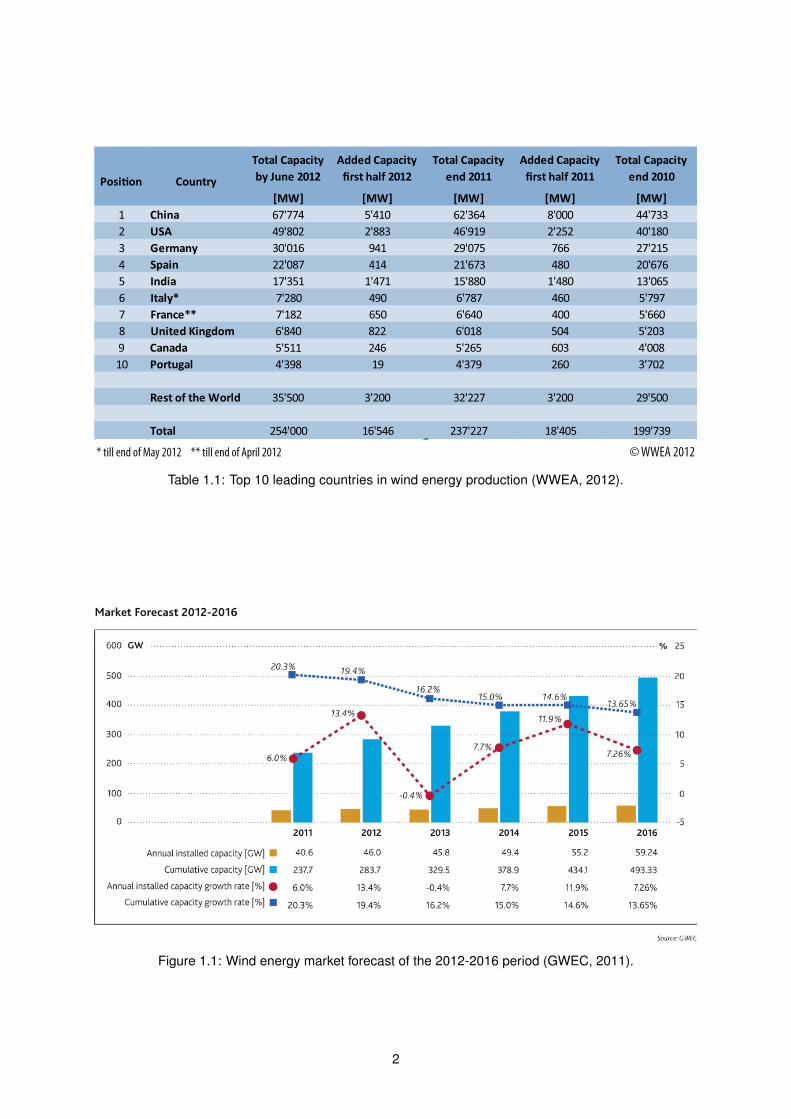
Nowadays, the use of wind power to generate electricity is widely spread across the world. In the last

few years, the worldwide wind energy production has been strongly increasing (see Tab. 1.1) and by the

end of June 2012, the total worldwide installed capacity reached 254 GW. China, the USA and Germany

lead the energy production capacity while Portugal occupies the 10th place, with a production capacity of

4398 MW (Tab. 1.1). This capacity is expected to keep increasing according to the forecast elaborated

by the Global Wind Energy Council presented on Fig. 1.1. Supporting this forecast are studies such as

Marvel et al. (2012), which claims that there is enough power in Earth’s winds to be a primary source

of near-zero-emission electric power as the global economy continues to grow through the twenty-first

century.

1

© WWEA 2012* till end of May 2012 ** till end of April 2012

Posi on Country

Total Capacity

by June 2012

Added Capacity

first half 2012

Total Capacity

end 2011

Added Capacity

first half 2011

Total Capacity

end 2010

[MW] [MW] [MW] [MW] [MW]

1 China 67'774 5'410 62'364 8'000 44'733

2 USA 49'802 2'883 46'919 2'252 40'180

3 Germany 30'016 941 29'075 766 27'215

4 Spain 22'087 414 21'673 480 20'676

5 India 17'351 1'471 15'880 1'480 13'065

6 Italy* 7'280 490 6'787 460 5'797

7 France** 7'182 650 6'640 400 5'660

8 United Kingdom 6'840 822 6'018 504 5'203

9 Canada 5'511 246 5'265 603 4'008

10 Portugal 4'398 19 4'379 260 3'702

Rest of the World 35'500 3'200 32'227 3'200 29'500

Total 254'000 16'546 237'227 18'405 199'739

Table 1.1: Top 10 leading countries in wind energy production (WWEA, 2012).

Figure 1.1: Wind energy market forecast of the 2012-2016 period (GWEC, 2011).

2

1.2 Environmental Impact of Wind Energy

All technologies have flaws and wind energy is no exception. Even being regarded in general as

environmentally friendly, wind farms have impact, and with the increase of the installation of wind turbines,

awareness towards them has also increased. The potential negative effects of wind energy can be divided

into the following categories:

• Avian / bat interaction;

• Visual impact;

• Wind turbine noise;

• Electromagnetic interference;

• Land-use impact;

• Other.

All these categories should be addressed in certain phases of a wind project and each one has its

own regulation, which varies from country to country or even from site to site.

The problem of wind turbine noise has been one of the most studied environmental impact subjects. It

is controversial as, although noise levels can be measured, its impact on the environment and the public’s

perception of the noise is partly subjective. There have been, however, many studies on the impact of

wind turbine noise on human health and wildlife (Stephens, 1982; Colby et al., 2009).

1.3 Legislation on WT Noise

As mentioned before, the legislation regarding noise varies from country to country, as a result of the

inexistence of common international noise standards or regulations for sound pressure levels. However,

the basics are the same: they establish maximum sound levels that can be produced for a particular

location (or type of location) and time of day (day/night). Taking Portugal as an example, the limits for

noise exposure according to it’s law are presented in Tab. 1.2.

Area type Lden (dB(A)) Ln (dB(A))

sensitive < 55 < 43mixed < 65 < 55not defined < 63 < 53

Table 1.2: Noise limits of sound pressure level according to the Portuguese legislation (Ministerio doAmbiente do Ordenamento do Territorio e do Desenvolvimento Regional, 2007).

There are three different zones defined by the Portuguese reference: sensitive areas, defined as being

oriented towards residential use, schools, hospitals, etc; mixed areas, which are defined as having the

same profile of the sensitive areas, with the exception of a clause allowing their use for other unplanned

purposes; and the areas which are neither sensitive, neither mixed, referred to as not defined. In the

table, two values are given: Lden, which is the averaged sound pressure level over a period of 24 hours,

and Ln, which is the sound pressure level during night time.

3

Other countries around Europe have similar limits of noise levels, as seen in Tab. 1.3.

Country Commercial Mixed Residential Rural

Denmark 40 45

Germanyday 65 60 55 50night 50 45 40 35

Netherlandsday 50 45 40night 40 35 30

Table 1.3: Noise limits of equivalent sound pressure levels Leq (dB(A)) in some European countries (Gipe,1995).

Sometimes a penalty of typically 5 dB(A) can be added to the noise limits, due to the tonal noise,

and the legislations also specify how the noise levels should be measured. In Wagner et al. (1996) and

Hubbard and Shepherd (1990) reviews of noise measurement techniques are given.

1.4 State of The Art

Noise Prediction Research on the prediction of noise generated by wind turbines has been done

for many years and bibliography listing technical papers on the subjects of wind turbine acoustics is

available (Hubbard and Shepherd, 1988). In Lowson (1993) a prediction model is presented, based on the

empirical models of Brooks et al. (1989) and Amiet (1975). Fuglsang and Madsen (1996) implemented

a wind turbine aeroacoustic noise prediction model, similar to Lowson’s, coupled with an aerodynamic

prediction model, having validated its predictions against measurement data from the Bonus Combi 300

kW and performed optimization of the geometry of the blade. Similar implementations of aeroacoustic

wind turbine were done by Zhu (2004), Leloudas (2006), Vanhaeverbeke (2007) and Vargas (2008). A

thorough description of the various different prediction models available is also presented in Wagner et al.

(1996).

Nowadays many codes exist that predict the noise of a wind turbine by computing all of its components,

such as the SILANT (Boorsma and Schepers, 2012), the IAGNOISE (Kamruzzaman et al., 2009) or

the FAST codes, to which a aeroacoustic prediction model was added by Moriarty and Migliore (2003).

Tickell et al. (2004) made a comparison of various other prediction codes available. Recent developments

in noise prediction include the use of Computational Fluid Dynamics (CFD) (Tadamasa and Zangeneh,

2011).

Noise Reduction The aim of every prediction codes is to be used in the reduction of wind turbine

noise. The project SIROCCO (Schepers et al., 2007) was developed with the aim to reduce wind-

turbine aerodynamic noise significantly while maintaining aerodynamic performance by designing new

aero-acoustically optimized airfoils whose measurements were used to validate the SILANT code.

While some works aimed to reduce the noise by changing the shape parameters of the blade

(Leloudas, 2006; Vesel Jr, 2009), other works performed optimization on the 2D airfoil shape to obtain

4

low noise airfoils (Bizzarrini et al., 2011; Coimbra, 2012; Gocmen and Ozerdem, 2012). Oerlemans et al.

(2009) presented acoustic measurement data showing that using acoustically optimized blades on a wind

turbine reduced the overall noise up to 0.5 dB and using trailing-edge serrations on the blade reduced the

noise levels up to 3.2 dB, without reducing the aerodynamic performance of the turbine.

1.5 Report Overview

This thesis consisted in the aeroacoustic optimization of wind turbine blades. For this, a wind turbine

aeroacoustic prediction code was developed which can be divided into three parts: the aerodynamic

prediction, the acoustic prediction and the geometry definition. The theory behind the developed code

is presented in chapters 2, 3 and 4, respectively. Each chapter starts with an introduction to the basic

concepts behind the theory followed by the description of the models. In chapter 5, a description of the

structure of the implemented code along with the features of the code is presented. The validation of the

code is also presented in chapter 5. The optimization framework developed is described in chapter 6 and

in chapter 7 the results of the optimizations are presented and discussed. The thesis ends in chapter 8

with overall conclusions and remarks, as well as future work options.

5

6

Chapter 2

Wind Turbine Aerodynamics

A wind turbine extracts mechanical energy from the kinetic energy of the wind by slowing down the

wind. It can either be a Horizontal-Axis Wind Turbine (HAWT) or a Vertical-Axis Wind Turbine (VAWT),

depending on either it rotates around its horizontal axis or vertical axis, respectively. In the present work,

only HAWTs will be treated.

If the mass of air passing through the turbine is assumed to be separated from the mass that does not

pass, the separated part of the flow field remains a long stream tube lying up and downstream of the

turbine. As the flow approaches the turbine, its velocity drops and, in order to compensate for this drop,

the stream tube expands (Fig. 2.1).

Many methods for computing the performance of wind turbine exist. In the 1930s, Betz and Glauert

derived the classical analysis method, the Blade Element Momentum (BEM) theory, which combines the

Blade Element and Momentum theories.

In this chapter, this theory is revisited, together with some more recent developed corrections. The

chapter ends with the introduction to some corrections to the aerodynamic data used in the theory.

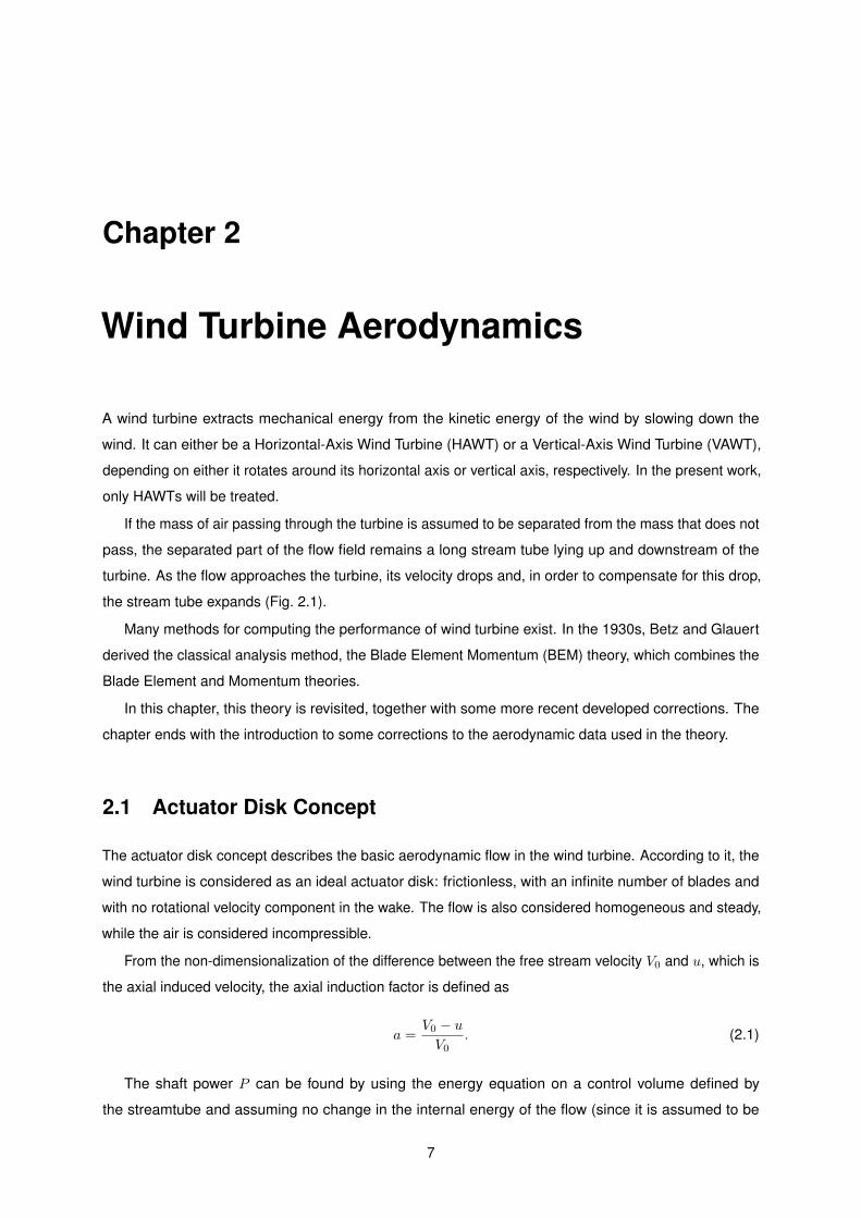
2.1 Actuator Disk Concept

The actuator disk concept describes the basic aerodynamic flow in the wind turbine. According to it, the

wind turbine is considered as an ideal actuator disk: frictionless, with an infinite number of blades and

with no rotational velocity component in the wake. The flow is also considered homogeneous and steady,

while the air is considered incompressible.

From the non-dimensionalization of the difference between the free stream velocity V0 and u, which is

the axial induced velocity, the axial induction factor is defined as

a =V0 − uV0

. (2.1)

The shaft power P can be found by using the energy equation on a control volume defined by

the streamtube and assuming no change in the internal energy of the flow (since it is assumed to be

7

Velocity

Pressure

u1u

0V 0p

0V

0p

Actuator Disk

0V

u

1u

0p

Figure 2.1: Actuator disk.

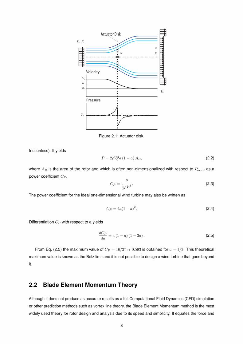
frictionless). It yields

P = 2ρV 20 a (1− a)AR, (2.2)

where AR is the area of the rotor and which is often non-dimensionalized with respect to Pavail as a

power coefficient CP ,

CP =P

12ρV

30

. (2.3)

The power coefficient for the ideal one-dimensional wind turbine may also be written as

CP = 4a(1− a)2. (2.4)

Differentiation CP with respect to a yields

dCPda

= 4 (1− a) (1− 3a) . (2.5)

From Eq. (2.5) the maximum value of CP = 16/27 ≈ 0.593 is obtained for a = 1/3. This theoretical

maximum value is known as the Betz limit and it is not possible to design a wind turbine that goes beyond

it.

2.2 Blade Element Momentum Theory

Although it does not produce as accurate results as a full Computational Fluid Dynamics (CFD) simulation

or other prediction methods such as vortex line theory, the Blade Element Momentum method is the most

widely used theory for rotor design and analysis due to its speed and simplicity. It equates the force and

8

torque relations derived from momentum theory and blade element theory in order to model the axial

and tangential induction factors, where the following assumptions are made: there is no aerodynamic

interaction between blade elements; the radial velocity component is ignored and the forces on the blade

element are functions only of the aerodynamics characteristics of the 2D airfoil of the element.

The full derivation of the BEM theory equations can be found in most wind turbine design handbooks

(Hansen, 2012; Burton et al., 2001) and only a summarized derivation of the method will be presented.

Rotor Plane

ωr(1 + a’)

V0(1 - a)

αθ

φ

Vrel

Lift

Drag

Fn

Ft

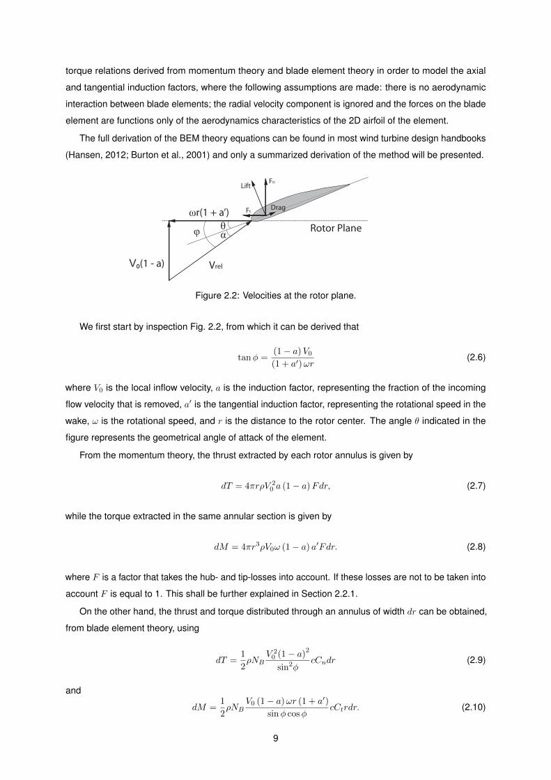
Figure 2.2: Velocities at the rotor plane.

We first start by inspection Fig. 2.2, from which it can be derived that

tanφ =(1− a)V0

(1 + a′)ωr(2.6)

where V0 is the local inflow velocity, a is the induction factor, representing the fraction of the incoming

flow velocity that is removed, a′ is the tangential induction factor, representing the rotational speed in the

wake, ω is the rotational speed, and r is the distance to the rotor center. The angle θ indicated in the

figure represents the geometrical angle of attack of the element.

From the momentum theory, the thrust extracted by each rotor annulus is given by

dT = 4πrρV 20 a (1− a)Fdr, (2.7)

while the torque extracted in the same annular section is given by

dM = 4πr3ρV0ω (1− a) a′Fdr. (2.8)

where F is a factor that takes the hub- and tip-losses into account. If these losses are not to be taken into

account F is equal to 1. This shall be further explained in Section 2.2.1.

On the other hand, the thrust and torque distributed through an annulus of width dr can be obtained,

from blade element theory, using

dT =1

2ρNB

V 20 (1− a)

2

sin2φcCndr (2.9)

and

dM =1

2ρNB

V0 (1− a)ωr (1 + a′)

sinφ cosφcCtrdr. (2.10)

9

where Cn and Ct are the coefficients of the resulting aerodynamic forces in the direction normal and

tangent to the rotor plane (see Fig. 2.2), NB is the number of blades and c is the chord of the element.

Equalizing Eq. (2.7) and Eq. (2.9) for dT , the expression for the axial induction factor a is obtained as

a =1

4F sin2φ

σCn+ 1

, (2.11)

where σ = c(r)NB/2πr is the local solidity. If Eq. (2.8) and Eq. (2.10) are equalized for dM , the expression

for a′ is obtained as

a′ =1

4F sinφ cosφ

σCt− 1

. (2.12)

2.2.1 Corrections to BEM theory

Tip Loss Model

The original blade element momentum theory does not account for the influence of the vortexes shed

from the blade tips into the wake on the induced velocity field. Prandtl derived a correction factor F to

compensate for this deficiency in BEM theory (Glauert, 1935) and it is computed as

F =2

πcos−1

(e−f

), (2.13)

where

f =NB2

R− rr sinφ

, (2.14)

where R is the blade radius and r the radius at a specific location.

Hub Loss Model

As there are also vortexes being shed near the hub of the rotor, another correction factor can also be

applied to correct the induced velocity. The hub-loss model is nearly identical to the tip-loss model, with

the following equation replacing Eq. (2.14):

f =NB2

r −Rhubr sinφ

. (2.15)

Each element of the blade can be affected by both the tip-loss and the hub-loss factors, with the total

factor being a multiplication of the tip-loss factor by the hub-loss factor.

F = FhubFtip (2.16)

Glauert Correction

As previously noted, the BEM theory is based on various assumptions, which exclude the 3D character-

istics of the flow, turbulence or separation. These assumptions work when the wind turbine is working

10

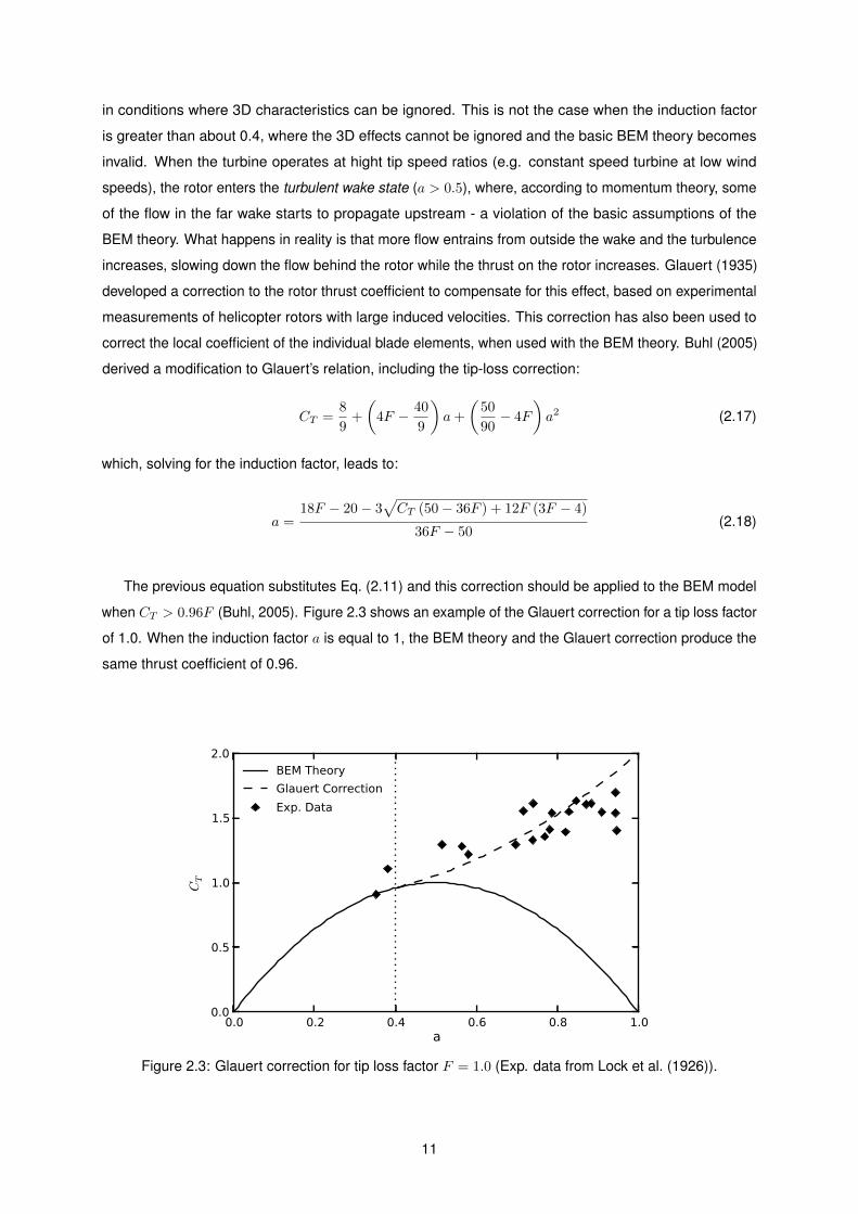
in conditions where 3D characteristics can be ignored. This is not the case when the induction factor

is greater than about 0.4, where the 3D effects cannot be ignored and the basic BEM theory becomes

invalid. When the turbine operates at hight tip speed ratios (e.g. constant speed turbine at low wind

speeds), the rotor enters the turbulent wake state (a > 0.5), where, according to momentum theory, some

of the flow in the far wake starts to propagate upstream - a violation of the basic assumptions of the

BEM theory. What happens in reality is that more flow entrains from outside the wake and the turbulence

increases, slowing down the flow behind the rotor while the thrust on the rotor increases. Glauert (1935)

developed a correction to the rotor thrust coefficient to compensate for this effect, based on experimental

measurements of helicopter rotors with large induced velocities. This correction has also been used to

correct the local coefficient of the individual blade elements, when used with the BEM theory. Buhl (2005)

derived a modification to Glauert’s relation, including the tip-loss correction:

CT =8

9+

(4F − 40

9

)a+

(50

90− 4F

)a2 (2.17)

which, solving for the induction factor, leads to:

a =18F − 20− 3

√CT (50− 36F ) + 12F (3F − 4)

36F − 50(2.18)

The previous equation substitutes Eq. (2.11) and this correction should be applied to the BEM model

when CT > 0.96F (Buhl, 2005). Figure 2.3 shows an example of the Glauert correction for a tip loss factor

of 1.0. When the induction factor a is equal to 1, the BEM theory and the Glauert correction produce the

same thrust coefficient of 0.96.

0.0 0.2 0.4 0.6 0.8 1.0a

0.0

0.5

1.0

1.5

2.0

CT

BEM Theory

Glauert Correction

Exp. Data

Figure 2.3: Glauert correction for tip loss factor F = 1.0 (Exp. data from Lock et al. (1926)).

11

2.2.2 Iteration Procedure

With all the necessary equations for the BEM model derived, the iteration procedure can be summarized.

This procedure is repeated for each element of the blade.

Step 1 Initialize a and a′ (usually a = a′ = 0).

Step 2 Compute the flow angle φ using Eq. (2.6)

Step 3 Compute the local angle of attack α with

α = φ− θ. (2.19)

Step 4 Obtain Cl and Cd from an aerodynamic table.

Step 5 Compute Cn and Ct.

Step 6 Compute the tip- and hub-loss corrections using Eq. (2.14) and Eq. (2.15).

Step 7 Compute the thrust coefficient for the element using

CT =σ(1− a)

2(Cl cosφ+ Cd sinφ)

sin2φ(2.20)

Step 8 Compute the axial induction a using Eq. (2.11), or, if CT > 0.96F , using Eq. (2.18).

Step 9 Compute tangential induction factor using Eq. (2.12).

Step 10 If a and a′ have changed more than a certain tolerance, go to Step 2 or else finish.

2.3 Annual Energy Production

With the wind turbine power curve (the shaft power as a function of the wind speed V0) obtained, it is then

possible to compute the annual energy production of the wind turbine. In order to do so, it is necessary to

combine this production curve with a probability density function h for the wind. Typically, the probability

density function of the wind is given by either a Rayleigh or a Weibull distribution (see Fig. 2.4). The

Weibull distribution can be modeled through of a scaling factor A and a form factor k:

hw (V0) =k

A

(V0

A

)k−1

exp

(−(V0

A

)k)(2.21)

From the Weibull distribution, the probability f (Vi < V0 < Vi+1) that the wind speed lies between Vi

and Vi+1 is given by

f (Vi < V0 < Vi+1) = exp

(−(ViA

)k)− exp

(−(Vi+1

A

)k). (2.22)

12

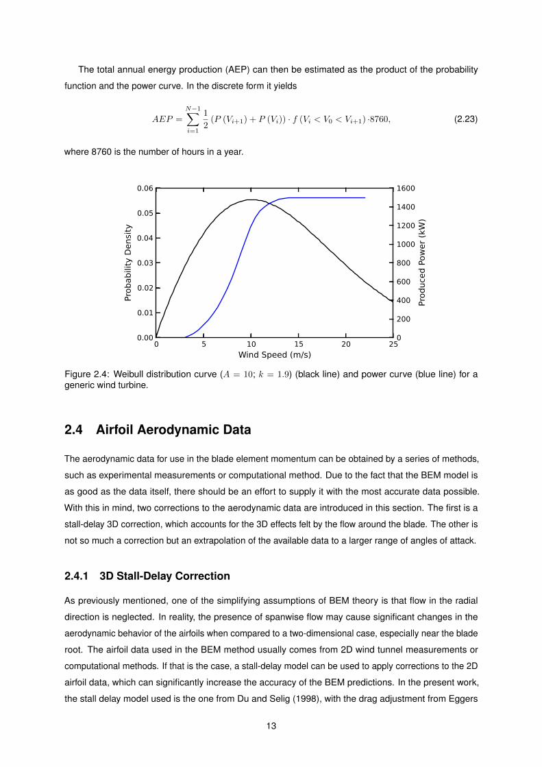
The total annual energy production (AEP) can then be estimated as the product of the probability

function and the power curve. In the discrete form it yields

AEP =

N−1∑i=1

1

2(P (Vi+1) + P (Vi)) · f (Vi < V0 < Vi+1) ·8760, (2.23)

where 8760 is the number of hours in a year.

0 5 10 15 20 25

Wind Speed (m/s)

0.00

0.01

0.02

0.03

0.04

0.05

0.06

Probability Density

0

200

400

600

800

1000

1200

1400

1600

Produced Power (kW)

Figure 2.4: Weibull distribution curve (A = 10; k = 1.9) (black line) and power curve (blue line) for ageneric wind turbine.

2.4 Airfoil Aerodynamic Data

The aerodynamic data for use in the blade element momentum can be obtained by a series of methods,

such as experimental measurements or computational method. Due to the fact that the BEM model is

as good as the data itself, there should be an effort to supply it with the most accurate data possible.

With this in mind, two corrections to the aerodynamic data are introduced in this section. The first is a

stall-delay 3D correction, which accounts for the 3D effects felt by the flow around the blade. The other is

not so much a correction but an extrapolation of the available data to a larger range of angles of attack.

2.4.1 3D Stall-Delay Correction

As previously mentioned, one of the simplifying assumptions of BEM theory is that flow in the radial

direction is neglected. In reality, the presence of spanwise flow may cause significant changes in the

aerodynamic behavior of the airfoils when compared to a two-dimensional case, especially near the blade

root. The airfoil data used in the BEM method usually comes from 2D wind tunnel measurements or

computational methods. If that is the case, a stall-delay model can be used to apply corrections to the 2D

airfoil data, which can significantly increase the accuracy of the BEM predictions. In the present work,

the stall delay model used is the one from Du and Selig (1998), with the drag adjustment from Eggers

13

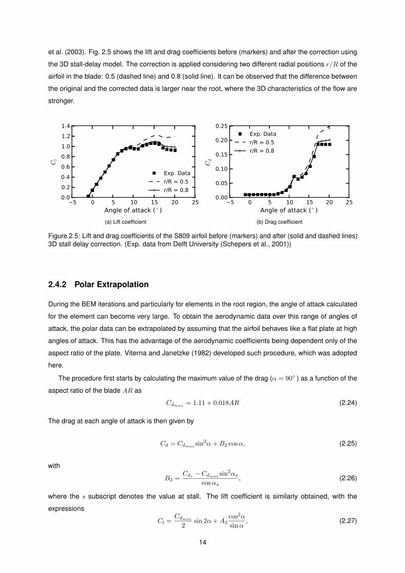
et al. (2003). Fig. 2.5 shows the lift and drag coefficients before (markers) and after the correction using

the 3D stall-delay model. The correction is applied considering two different radial positions r/R of the

airfoil in the blade: 0.5 (dashed line) and 0.8 (solid line). It can be observed that the difference between

the original and the corrected data is larger near the root, where the 3D characteristics of the flow are

stronger.

−5 0 5 10 15 20 25

Angle of attack ( ◦ )

0.0

0.2

0.4

0.6

0.8

1.0

1.2

1.4

Cl

Exp. Data

r/R = 0.5

r/R = 0.8

(a) Lift coefficient

−5 0 5 10 15 20 25

Angle of attack ( ◦ )

0.00

0.05

0.10

0.15

0.20

0.25

Cd

Exp. Data

r/R = 0.5

r/R = 0.8

(b) Drag coefficient

Figure 2.5: Lift and drag coefficients of the S809 airfoil before (markers) and after (solid and dashed lines)3D stall delay correction. (Exp. data from Delft University (Schepers et al., 2001))

2.4.2 Polar Extrapolation

During the BEM iterations and particularly for elements in the root region, the angle of attack calculated

for the element can become very large. To obtain the aerodynamic data over this range of angles of

attack, the polar data can be extrapolated by assuming that the airfoil behaves like a flat plate at high

angles of attack. This has the advantage of the aerodynamic coefficients being dependent only of the

aspect ratio of the plate. Viterna and Janetzke (1982) developed such procedure, which was adopted

here.

The procedure first starts by calculating the maximum value of the drag (α = 90◦ ) as a function of the

aspect ratio of the blade AR as

Cdmax = 1.11 + 0.018AR (2.24)

The drag at each angle of attack is then given by

Cd = Cdmaxsin2α+B2 cosα, (2.25)

with

B2 =Cds − Cdmaxsin2αs

cosαs, (2.26)

where the s subscript denotes the value at stall. The lift coefficient is similarly obtained, with the

expressions

Cl =Cdmax

2sin 2α+A2

cos2α

sinα, (2.27)

14

and

A2 = (Cls − Cdmax sinαs cosαs)sinαscos2αs

. (2.28)

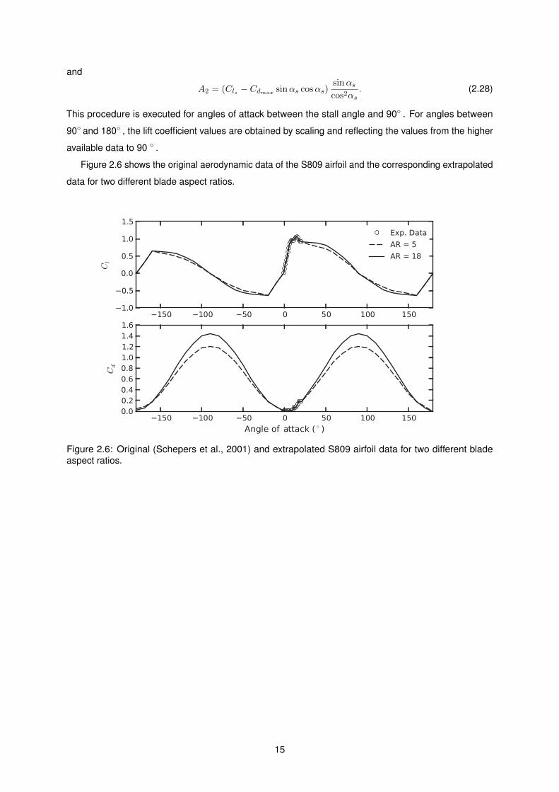
This procedure is executed for angles of attack between the stall angle and 90◦ . For angles between

90◦ and 180◦ , the lift coefficient values are obtained by scaling and reflecting the values from the higher

available data to 90 ◦ .

Figure 2.6 shows the original aerodynamic data of the S809 airfoil and the corresponding extrapolated

data for two different blade aspect ratios.

Figure 2.6: Original (Schepers et al., 2001) and extrapolated S809 airfoil data for two different bladeaspect ratios.

15

16

Chapter 3

Noise from Wind Turbines

In this chapter, the theory behind the generation of noise from a wind turbine is presented. It starts with a

brief introduction to some key concepts followed by a description of the wind turbine noise generation

mechanisms. It ends with the description of the noise prediction model developed in this work.

3.1 Principles of Acoustics

Sound is an oscillation of pressure propagating through a medium as sound waves. It can be generated

by various different mechanisms. Some well-known examples are the loudspeaker, where the sound

is produced by a vibrating surface, or the siren, where the sound is created by the periodic injection

of air. The sound waves are characterized in terms of their wavelength λ, frequency f , and velocity

c0 (approximately 340 m/s in air, at standard conditions). After being partially absorbed, reflected or

attenuated, these waves may reach the human eardrum of an observer, where they produce a sensation

of hearing, depending on the amplitude of the sound wave. This sensation might turn the sound into

noise, if it is considered unwanted. The classification of sound as noise is very subjective as it depends

on factors such as the sensitivity of the listener and the situation, as well as measurable quantities like

level and duration.

In this section, only some basic concepts are introduced and a reader less familiar with the aeroa-

coustic fundamental theories of aeroacoustics should refer to available literature such as (Lau, 2011) or

(Goldstein, 1976).

3.1.1 Sound Pressure and Power Levels

The response of the human ear to the amplitude of sound pressure is not linear. For example, if the

amplitude of the sound pressure is doubled it produces a sensation of a louder sound, however, it seems

far less than twice as loud. This leads to the definition of a logarithmic scale to characterize sound

pressure amplitudes, as it approximates the actual response of the human ear. The sound pressure level

17

Lp is expressed in deciBel ( dB) and can be defined as

Lp = 10log10

(p2rms

p2ref

), (3.1)

where pref is a reference pressure (usually 20 × 10−5 Pa), and prms is the root mean square sound

pressure defined by

p2rms = lim

T→∞

(1

T

∫ T

0

p2(t)dt

). (3.2)

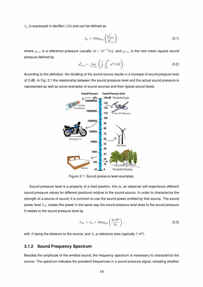
According to this definition, the doubling of the sound source results in a increase of sound pressure level

of 3 dB. In Fig. 3.1 the relationship between the sound pressure level and the actual sound pressure is

represented as well as some examples of sound sources and their typical sound levels.

140 dB

130

120

110

100

90

80

70

60

50

40

30

20

10

0

μPa100000000

10000000

1000000

100000

10000

1000

100

20 Threshold of hearing

Threshold of pain

Sound Pressure Sound Pressure level

Jet take-o! (100m away)

Bedroom

Jet Engine

(25 m distance)

Wind Turbine

Motorcycle at 1 m

Figure 3.1: Sound pressure level examples.

Sound pressure level is a property of a field position, this is, an observer will experience different

sound pressure values for different positions relative to the sound source. In order to characterize the

strength of a source of sound, it is common to use the sound power emitted by that source. The sound

power level LW scales this power in the same way the sound pressure level does to the sound pressure.

It relates to the sound pressure level by

LW = Lp + 10log10

(4πR2

S0

), (3.3)

with R being the distance to the source, and S0 a reference area (typically 1 m2).

3.1.2 Sound Frequency Spectrum

Besides the amplitude of the emitted sound, the frequency spectrum is necessary to characterize the

source. The spectrum indicates the prevalent frequencies in a sound pressure signal, revealing whether

18

Frequency (Hz)

Ga

in (

dB

)

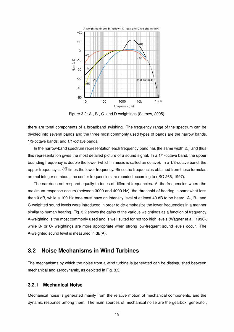
Figure 3.2: A-, B-, C- and D-weightings (Skirrow, 2005).

there are tonal components of a broadband swishing. The frequency range of the spectrum can be

divided into several bands and the three most commonly used types of bands are the narrow bands,

1/3-octave bands, and 1/1-octave bands.

In the narrow-band spectrum representation each frequency band has the same width ∆f and thus

this representation gives the most detailed picture of a sound signal. In a 1/1-octave band, the upper

bounding frequency is double the lower (which in music is called an octave). In a 1/3-octave band, the

upper frequency is 3√

2 times the lower frequency. Since the frequencies obtained from these formulas

are not integer numbers, the center frequencies are rounded according to (ISO 266, 1997).

The ear does not respond equally to tones of different frequencies. At the frequencies where the

maximum response occurs (between 3000 and 4000 Hz), the threshold of hearing is somewhat less

than 0 dB, while a 100 Hz tone must have an intensity level of at least 40 dB to be heard. A-, B-, and

C-weighted sound levels were introduced in order to de-emphasize the lower frequencies in a manner

similar to human hearing. Fig. 3.2 shows the gains of the various weightings as a function of frequency.

A-weighting is the most commonly used and is well suited for not too high levels (Wagner et al., 1996),

while B- or C- weightings are more appropriate when strong low-frequent sound levels occur. The

A-weighted sound level is measured in dB(A).

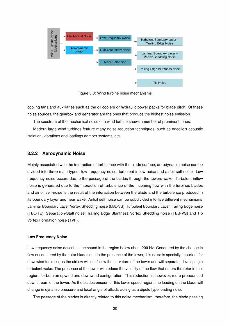
3.2 Noise Mechanisms in Wind Turbines

The mechanisms by which the noise from a wind turbine is generated can be distinguished between

mechanical and aerodynamic, as depicted in Fig. 3.3.

3.2.1 Mechanical Noise

Mechanical noise is generated mainly from the relative motion of mechanical components, and the

dynamic response among them. The main sources of mechanical noise are the gearbox, generator,

19

Mechanical Noise

Aerodynamic

Noise

Low Frequency Noise

Turbulent Inflow Noise

Airfoil Self-noise

Turbulent Boundary Layer –

Trailing Edge Noise

Laminar Boundary Layer –

Vortex Shedding Noise

Trailing Edge Bluntness Noise

Tip Noise

Win

d T

urb

ine

No

ise

Me

ch

an

ism

s

Figure 3.3: Wind turbine noise mechanisms.

cooling fans and auxiliaries such as the oil coolers or hydraulic power packs for blade pitch. Of these

noise sources, the gearbox and generator are the ones that produce the highest noise emission.

The spectrum of the mechanical noise of a wind turbine shows a number of prominent tones.

Modern large wind turbines feature many noise reduction techniques, such as nacelle’s acoustic

isolation, vibrations and loadings damper systems, etc.

3.2.2 Aerodynamic Noise

Mainly associated with the interaction of turbulence with the blade surface, aerodynamic noise can be

divided into three main types: low frequency noise, turbulent inflow noise and airfoil self-noise. Low

frequency noise occurs due to the passage of the blades through the towers wake. Turbulent inflow

noise is generated due to the interaction of turbulence of the incoming flow with the turbines blades

and airfoil self-noise is the result of the interaction between the blade and the turbulence produced in

its boundary layer and near wake. Airfoil self noise can be subdivided into five different mechanisms:

Laminar Boundary Layer Vortex Shedding noise (LBL-VS), Turbulent Boundary Layer Trailing Edge noise

(TBL-TE), Separation-Stall noise, Trailing Edge Bluntness Vortex Shedding noise (TEB-VS) and Tip

Vortex Formation noise (TVF).

Low Frequency Noise

Low frequency noise describes the sound in the region below about 200 Hz. Generated by the change in

flow encountered by the rotor blades due to the presence of the tower, this noise is specially important for

downwind turbines, as the airflow will not follow the curvature of the tower and will separate, developing a

turbulent wake. The presence of the tower will reduce the velocity of the flow that enters the rotor in that

region, for both an upwind and downwind configuration. This reduction is, however, more pronounced

downstream of the tower. As the blades encounter this lower speed region, the loading on the blade will

change in dynamic pressure and local angle of attack, acting as a dipole type loading noise.

The passage of the blades is directly related to this noise mechanism, therefore, the blade passing

20

frequency fB and its harmonics fb, which are functions of the rotor frequency fR, dominate the spectrum.

fB = nB · fR (3.4)

fb = n · fB (3.5)

For wind turbines, fB is typically in the order of 1-3 Hz and this low frequency noise contributes only

to the low frequency part of the wind turbine noise spectrum.

Nowadays, most wind turbines have an upwind configuration and the ones with a downwind configura-

tion incorporate design features that reduce impulsive noise, such as the positioning of the rotor further

away from the tower. Moreover, due to low rotor frequencies, low frequency noise is not an important part

of the spectrum of large wind turbines. It may, however, become important for small wind turbines with

higher rotational speeds, where the passing frequency and its harmonics may shift to the audible part of

the spectrum.

Turbulent Inflow Noise

When atmospheric turbulence encounters the blade, it causes a broadband noise radiation, called

turbulent inflow noise.

There are two causes for atmospheric turbulence: aerodynamic and thermal. Aerodynamic turbulence

is generated by the interaction of the flow with the ground surface, while thermal turbulence is generated

by the buoyancy of the air due to local heating by the sun. The two most important characteristics of

turbulence are turbulence intensity, which indicates the turbulence fluctuations and is defined as the ratio

of the standard deviation and the averaged mean wind velocity, and the turbulence length scale, which

indicates the size of the eddies.

The size of the eddies is related to the frequency of the generated noise by this mechanism. Eddies

larger than the airfoil chord will generate low frequency noise as it changes the airfoil loading as a whole

while eddies smaller than the airfoil chord will induce localized pressure fluctuations, thus producing high

frequency noise.

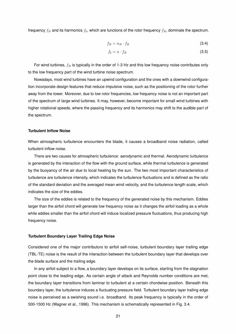
Turbulent Boundary Layer Trailing Edge Noise

Considered one of the major contributors to airfoil self-noise, turbulent boundary layer trailing edge

(TBL-TE) noise is the result of the interaction between the turbulent boundary layer that develops over

the blade surface and the trailing edge.

In any airfoil subject to a flow, a boundary layer develops on its surface, starting from the stagnation

point close to the leading edge. As certain angle of attack and Reynolds number conditions are met,

the boundary layer transitions from laminar to turbulent at a certain chordwise position. Beneath this

boundary layer, the turbulence induces a fluctuating pressure field. Turbulent boundary layer trailing edge

noise is perceived as a swishing sound i.e. broadband. Its peak frequency is typically in the order of

500-1500 Hz (Wagner et al., 1996). This mechanism is schematically represented in Fig. 3.4.

21

boundary layer

Turbulent Eddies passing

the trailing edge

Sound radiated from

the trailing edge

Figure 3.4: Representation of the TBL-TE noise mechanism.

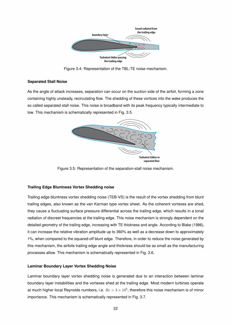
Separated Stall Noise

As the angle of attack increases, separation can occur on the suction side of the airfoil, forming a zone

containing highly unsteady, recirculating flow. The shedding of these vortices into the wake produces the

so called separated stall noise. This noise is broadband with its peak frequency typically intermediate to

low. This mechanism is schematically represented in Fig. 3.5.

Turbulent Eddies in

separated !ow

Figure 3.5: Representation of the separation-stall noise mechanism.

Trailing Edge Bluntness Vortex Shedding noise

Trailing edge bluntness vortex shedding noise (TEB-VS) is the result of the vortex shedding from blunt

trailing edges, also known as the van Karman type vortex sheet. As the coherent vortexes are shed,

they cause a fluctuating surface pressure differential across the trailing edge, which results in a tonal

radiation of discreet frequencies at the trailing edge. This noise mechanism is strongly dependent on the

detailed geometry of the trailing edge, increasing with TE thickness and angle. According to Blake (1986),

it can increase the relative vibration amplitude up to 360% as well as a decrease down to approximately

1%, when compared to the squared-off blunt edge. Therefore, in order to reduce the noise generated by

this mechanism, the airfoils trailing edge angle and thickness should be as small as the manufacturing

processes allow. This mechanism is schematically represented in Fig. 3.6.

Laminar Boundary Layer Vortex Shedding Noise

Laminar boundary layer vortex shedding noise is generated due to an interaction between laminar

boundary layer instabilities and the vortexes shed at the trailing edge. Most modern turbines operate

at much higher local Reynolds numbers, i.e. Re > 3× 106, therefore this noise mechanism is of minor

importance. This mechanism is schematically represented in Fig. 3.7.

22

boundary layertonal noise radiated from

trailing edge

vortex shedding from

blunt trailing edge

Figure 3.6: Representation of the TEB-VS noise mechanism.

boundary layerinstabilities in the

boundary layer

wake instabilities

Sound radiated from

the trailing edge

Figure 3.7: Representation of the LBL-VS noise mechanism.

Tip Vortex Formation Noise

Tip vortex formation noise is the noise generated, according to Brooks et al. (1989), due to the interaction

between the vortexes shed from the tip of the blade and the tip surface, in a way analogous to the TBL-TE

noise mechanism. The vortexes are shed due to the difference in pressure between the suction and

pressure sides of the blade. This noise is of broadband nature, and its level is strongly dependent on the

geometry of the tip. This mechanism is schematically represented in Fig. 3.8.

Sound radiated from

tip side edge

blade tip section

sound radiated from

trailing edge

tip vortexturbulent vortex core

Figure 3.8: Representation of the tip vortex formation noise mechanism.

3.3 Noise Prediction Model

The wind turbine noise prediction method developed in this work consists in dividing the turbine blade into

segments, much like what is done in the BEM theory for aerodynamic prediction of a wind turbine. This

way, each segment is considered to have a certain airfoil shape and span length. The noise radiation

process for any blade section can, according to Lowson (1993), be assumed as identical to that for an

equivalent airfoil section. Therefore, the sound pressure level can be computed at each blade noise

23

element and the total sound power level generated by the rotor is the result of a summation of the noise

from each blade element,

Ljp,total = 10log10

(NBNaz

∑i

10

Ljp,i

10

), (3.6)

where NB is the number of blades, Naz is the number of azimuthal positions where the blade is computed

and Ljp,i is the total sound pressure level generated by the ith blade noise element at frequency band j.

The total sound levels at each frequency band can also be summed,

Lp,overall = 10log10

∑j

10

Ljp,total

10

, (3.7)

thus leading to the Overall Sound Pressure Level (OASPL).

The model is limited to the rotor, since it is the object of interest. Therefore, noise contributions

from the interaction with the tower and nacelle are not taken into account, nor are mechanical noises

considered.

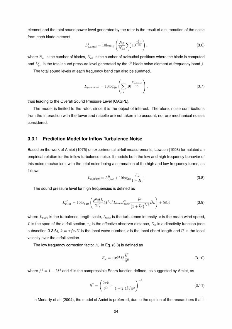
3.3.1 Prediction Model for Inflow Turbulence Noise

Based on the work of Amiet (1975) on experimental airfoil measurements, Lowson (1993) formulated an

empirical relation for the inflow turbulence noise. It models both the low and high frequency behavior of

this noise mechanism, with the total noise being a summation of the high and low frequency terms, as

follows

Lp,inflow = LHp,inf + 10log10

Kc

1 +Kc. (3.8)

The sound pressure level for high frequencies is defined as

LHp,inf = 10log10

(ρ2c20L

2r2e

M3u2LturbI2turb

k3(1 + k2

)7/3 Dh

)+ 58.4 (3.9)

where Lturb is the turbulence length scale, Iturb is the turbulence intensity, u is the mean wind speed,

L is the span of the airfoil section, re is the effective observer distance, Dh is a directivity function (see

subsection 3.3.6), k = πfc/U is the local wave number, c is the local chord length and U is the local

velocity over the airfoil section.

The low frequency correction factor Kc in Eq. (3.8) is defined as

Kc = 10S2Mk2

β2, (3.10)

where β2 = 1−M2 and S is the compressible Sears function defined, as suggested by Amiet, as

S2 =

(2πk

β2+

1

1 + 2.4k/β2

)−1

(3.11)

In Moriarty et al. (2004), the model of Amiet is preferred, due to the opinion of the researchers that it

24

is more reliable. In Amiet’s model, Eq. (3.8) is replaced by

LHp,inf = 10log10

ρ2c40L

2r2e

M5LturbI2turb

k3(1 + k2

)7/3Dh

+ 78.4 (3.12)

where k = k/ke is the wave number k = 2πf/U normalized by the wave number range of energy-

containing eddies ke = 3/ (4Lturb). Moriarty et al. also propose the use of a correction factor which

corrects the minor effect of the angle of attack on the turbulent inflow noise. The new correction factor is

given by

Kc = 10S2Mk2

β2

(1− α2

), (3.13)

with α being the angle of attack given in radians.

Prediction of Turbulence Parameters

Prediction of the turbulence characteristics is of great importance to this model. The intensity of the

turbulence and its length scale are dependent on the evaluation height (relative to the ground), the

roughness of the ground and on the meteorological conditions at the evaluated site. Some examples of

typical roughness lengths and their associated terrain types are presented on Tab. 3.1.

The mean wind speed also varies with height, and can be described with the power law relationship

Vz = Vref

(z

Href

)γ, (3.14)

where z is the height, Href is the reference height at which the velocity was measured, and γ is the power

law factor. This power law factor is a function of the surface roughness length z0 and its estimate is given

by Counihan (1975) as

γ = 0.24 + 0.096log10z0 + 0.016(log10z0)2. (3.15)

Turbulence intensity can be obtained using the relationship given by Snyder (1981), which is a function

of the height z, the ground roughness z0 and the power law factor γ,

Iturb = γln (30/z0)

ln (z/z0). (3.16)

The turbulence length scale is formulated as

Lturb = 25z0.35z−0.0630 . (3.17)

Correction to the Model

Being based on the flow over a flat plate, one of the main limitations of this prediction model is that it does

not account for the geometry of the airfoil. In their work, Moriarty et al. (2004) present a very complete

25

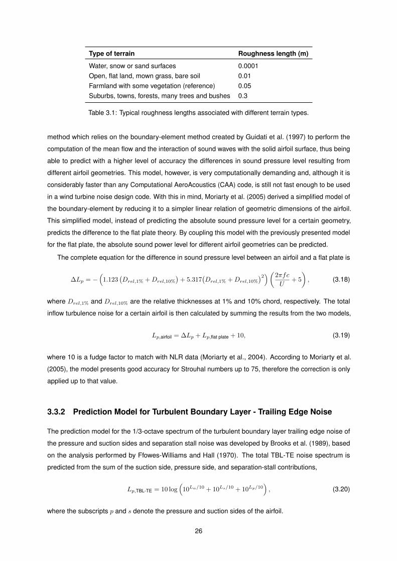
Type of terrain Roughness length (m)

Water, snow or sand surfaces 0.0001Open, flat land, mown grass, bare soil 0.01Farmland with some vegetation (reference) 0.05Suburbs, towns, forests, many trees and bushes 0.3

Table 3.1: Typical roughness lengths associated with different terrain types.

method which relies on the boundary-element method created by Guidati et al. (1997) to perform the

computation of the mean flow and the interaction of sound waves with the solid airfoil surface, thus being

able to predict with a higher level of accuracy the differences in sound pressure level resulting from

different airfoil geometries. This model, however, is very computationally demanding and, although it is

considerably faster than any Computational AeroAcoustics (CAA) code, is still not fast enough to be used

in a wind turbine noise design code. With this in mind, Moriarty et al. (2005) derived a simplified model of

the boundary-element by reducing it to a simpler linear relation of geometric dimensions of the airfoil.

This simplified model, instead of predicting the absolute sound pressure level for a certain geometry,

predicts the difference to the flat plate theory. By coupling this model with the previously presented model

for the flat plate, the absolute sound power level for different airfoil geometries can be predicted.

The complete equation for the difference in sound pressure level between an airfoil and a flat plate is

∆Lp = −(

1.123(Drel,1% +Drel,10%

)+ 5.317

(Drel,1% +Drel,10%

)2)(2πfc

U+ 5

), (3.18)

where Drel,1% and Drel,10% are the relative thicknesses at 1% and 10% chord, respectively. The total

inflow turbulence noise for a certain airfoil is then calculated by summing the results from the two models,

Lp,airfoil = ∆Lp + Lp,flat plate + 10, (3.19)

where 10 is a fudge factor to match with NLR data (Moriarty et al., 2004). According to Moriarty et al.

(2005), the model presents good accuracy for Strouhal numbers up to 75, therefore the correction is only

applied up to that value.

3.3.2 Prediction Model for Turbulent Boundary Layer - Trailing Edge Noise

The prediction model for the 1/3-octave spectrum of the turbulent boundary layer trailing edge noise of

the pressure and suction sides and separation stall noise was developed by Brooks et al. (1989), based

on the analysis performed by Ffowes-Williams and Hall (1970). The total TBL-TE noise spectrum is

predicted from the sum of the suction side, pressure side, and separation-stall contributions,

Lp,TBL-TE = 10 log(

10Lα/10 + 10Ls/10 + 10Lp/10), (3.20)

where the subscripts p and s denote the pressure and suction sides of the airfoil.

26

The pressure side contribution to this noise is given by

Lp,p = 10 log

(δ∗pM

5LDh

r2e

)+A

(StpSt1

)+ (K1 − 3) + ∆K1, (3.21)

the suction side by

Lp,s = 10 log

(δ∗sM

5LDh

r2e

)+A

(StsSt1

)+ (K1 − 3) , (3.22)

and the separation-stall contribution by

Lp,α = 10 log

(δ∗sM

5LDh

r2e

)+B

(StsSt2

)+K2, (3.23)

where δ∗ is the boundary layer displacement thickness and A and B are empirical spectral shape functions

based on the Strouhal number, defined in Appendix B.

For angles of attack higher than 12.5◦ , which is the stall angle for the NACA 0012 airfoil, the TBL-TE

noise source is mainly the separation-stall noise and equations (3.21) to (3.23) are replaced by

Lp,p = −∞, (3.24)

Lp,s = −∞, (3.25)

and

Lp,α = 10 log

(δ∗sM

5LD`

r2e

)+A′

(StsSt2

)+K2, (3.26)

where A′ is the shape function A for a Reynolds number three times the actual Reynolds number.

The Strouhal number definitions are

Stp =fδ∗pU, (3.27)

Sts =fδ∗sU, (3.28)

St1 = 0.02M−0.6, (3.29)

and

St2 = St1 ×

1

100.0054(α∗−1.33)2

4.72

(α∗ < 1.33)

(1.33 6 α∗ 6 12.5)

(12.5 < α∗)

(3.30)

where f is the frequency and U is the local mean velocity.

3.3.3 Prediction Model for the Laminar Boundary Layer - Vortex Shedding Noise

The scaling approach taken in (Brooks et al., 1989) for the LBL-VS noise is similar to that taken for the

TBL-TE noise with the difference that, instead of being a function of the boundary layer displacement

thickness (among other parameters), the LBL-VS prediction model is a function of the boundary layer

27

thickness δp at the pressure side. The noise spectrum in a 1/3 octave presentation is predicted by

LLBL-VS = 10 log

(δpM

5LDh

r2e

)+G1

(St′

St ′peak

)+G2

[Rc

(Rc)0

]+G3 (α∗) , (3.31)

where G1, G2 and G3 are spectral shape functions, defined in Appendix B.

The Strouhal definitions are

St′ =fδpU, (3.32)

and

St ′peak = St ′1 × 10−0.04α∗ , (3.33)

where

St ′1 =

0.18

0.001756R0.3931c

0.28

(Rc 6 1.3× 105

)(1.3× 105 6 Rc 6 4.0× 105

)(4.0× 105 < Rc

) . (3.34)

3.3.4 Prediction Model for Trailing Edge Bluntness Vortex Shedding Noise

Based on the same scaling method as the TBL-TE and LBL-VS noise, the prediction model for the

TEB-VS noise derives from an experiment by Brooks and Hodgson (1981). Its spectrum in a 1/3-octave

presentation is predicted by

LBLUNT = 10 log

(hM5.5LDh

r2e

)+G4

(h

δ∗avg,Ψ

)+G5

(h

δ∗avg,Ψ,

S t′′′

S t′′′peak

), (3.35)

where h is the bluntness thickness and δ∗avg = (δ∗p + δ∗s )/2 is the average boundary layer displacement

thickness.

The Strouhal number here is defined with the bluntness thickness instead of a boundary layer thickness

parameter.

S t′′′ =fh

U. (3.36)

The peak Strouhal number is defined as a function of the thickness ratio h/δ∗ and the trailing edge

angle Ψ,

S t′′′peak =

0.212− 0.0045Ψ

1 + 0.235(h/δ∗avg

)−1 − 0.0132(h/δ∗avg

)−2

(0.2 6 h/δ∗avg

)0.1(h/δ∗avg

)+ 0.095− 0.00243Ψ

(h/δ∗avg < 0.2

) . (3.37)

The function G4 determines the peak level of the spectrum and is given by

G4

(h/δ∗avg,Ψ

)=

17.5 log

(h/δ∗avg

)+ 157.5− 1.114Ψ

(h/δ∗avg 6 5

)169.7− 1.114Ψ

(5 < h/δ∗avg

) , (3.38)

28

while the spectral curve fitting function G5 is predicted as an interpolation between Ψ = 14◦ and Ψ = 0◦ ,

G5

(h

δ∗avg,Ψ,

S t′′′

S t′′′peak

)= (G5)Ψ=0◦ + 0.0714Ψ [(G5)Ψ=14◦ − (G5)Ψ=0◦ ] . (3.39)

The definition of functions (G5)Ψ=0◦ and (G5)Ψ=14◦ is presented in Appendix B.

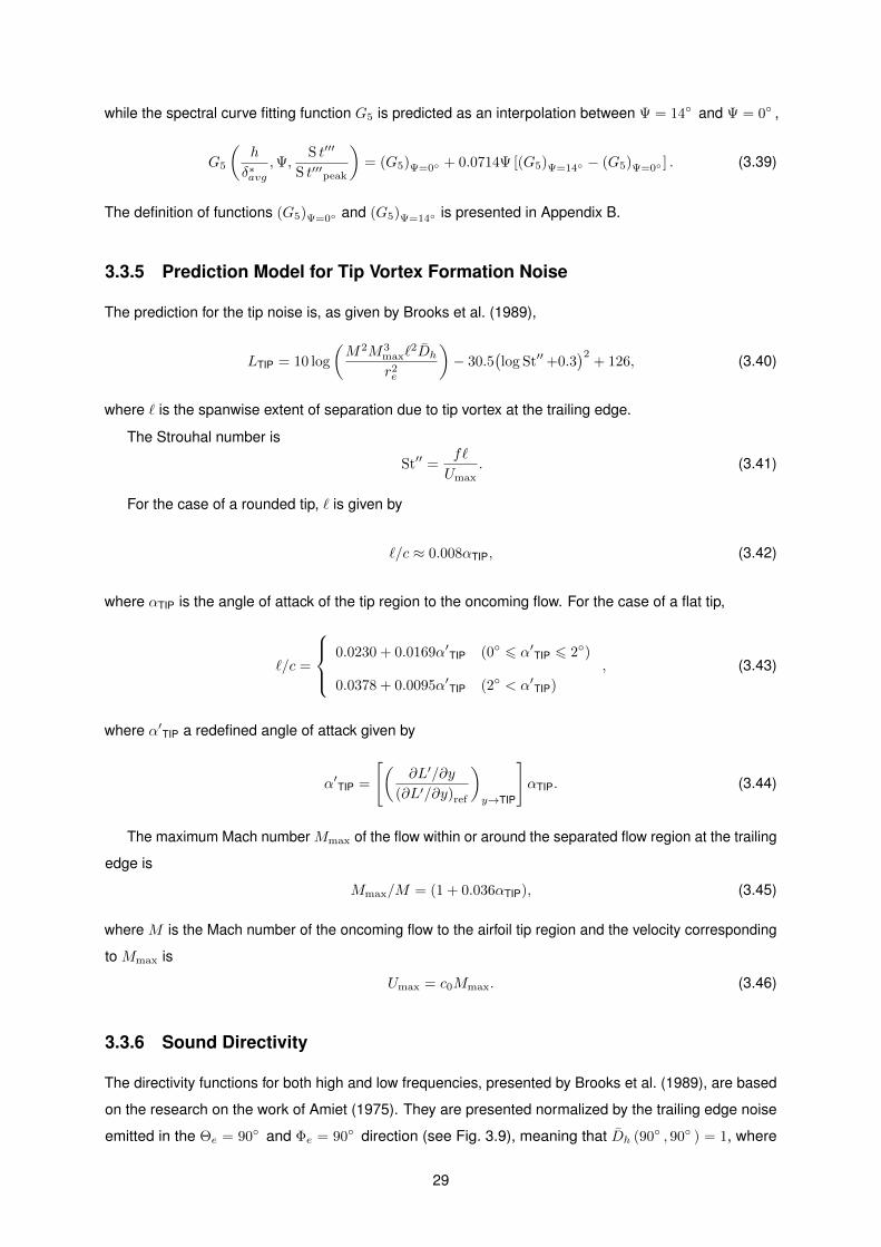
3.3.5 Prediction Model for Tip Vortex Formation Noise

The prediction for the tip noise is, as given by Brooks et al. (1989),

LTIP = 10 log

(M2M3

max`2Dh

r2e

)− 30.5

(log St′′+0.3

)2+ 126, (3.40)

where ` is the spanwise extent of separation due to tip vortex at the trailing edge.

The Strouhal number is

St′′ =f`

Umax. (3.41)

For the case of a rounded tip, ` is given by

`/c ≈ 0.008αTIP, (3.42)

where αTIP is the angle of attack of the tip region to the oncoming flow. For the case of a flat tip,

`/c =

0.0230 + 0.0169α′TIP (0◦ 6 α′TIP 6 2◦)

0.0378 + 0.0095α′TIP (2◦ < α′TIP)

, (3.43)

where α′TIP a redefined angle of attack given by

α′TIP =

[(∂L′/∂y

(∂L′/∂y)ref

)y→TIP

]αTIP. (3.44)

The maximum Mach number Mmax of the flow within or around the separated flow region at the trailing

edge is

Mmax/M = (1 + 0.036αTIP), (3.45)

where M is the Mach number of the oncoming flow to the airfoil tip region and the velocity corresponding

to Mmax is

Umax = c0Mmax. (3.46)

3.3.6 Sound Directivity

The directivity functions for both high and low frequencies, presented by Brooks et al. (1989), are based

on the research on the work of Amiet (1975). They are presented normalized by the trailing edge noise

emitted in the Θe = 90◦ and Φe = 90◦ direction (see Fig. 3.9), meaning that Dh (90◦ , 90◦ ) = 1, where

29

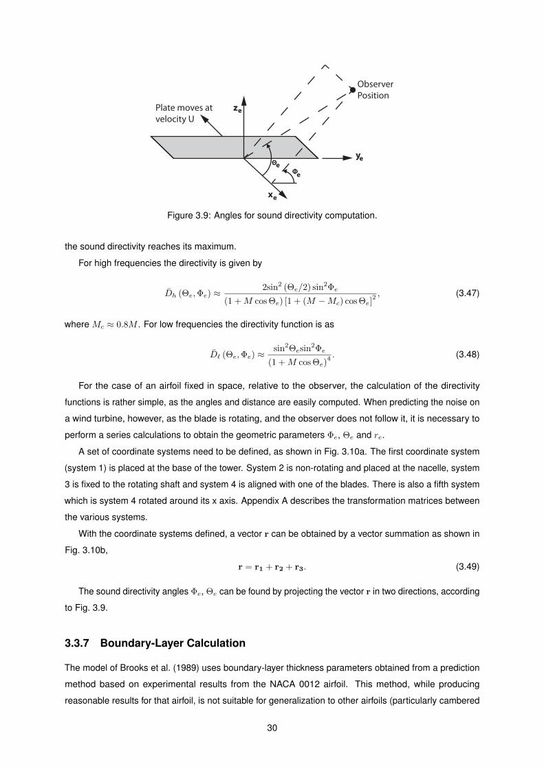
Θye

xe

ze

Φe

Plate moves at

velocity U

Observer

Position

e

Figure 3.9: Angles for sound directivity computation.

the sound directivity reaches its maximum.

For high frequencies the directivity is given by

Dh (Θe,Φe) ≈2sin2 (Θe/2) sin2Φe

(1 +M cos Θe) [1 + (M −Mc) cos Θe]2 , (3.47)

where Mc ≈ 0.8M . For low frequencies the directivity function is as

D` (Θe,Φe) ≈sin2Θesin

2Φe

(1 +M cos Θe)4 . (3.48)

For the case of an airfoil fixed in space, relative to the observer, the calculation of the directivity

functions is rather simple, as the angles and distance are easily computed. When predicting the noise on

a wind turbine, however, as the blade is rotating, and the observer does not follow it, it is necessary to

perform a series calculations to obtain the geometric parameters Φe, Θe and re.

A set of coordinate systems need to be defined, as shown in Fig. 3.10a. The first coordinate system

(system 1) is placed at the base of the tower. System 2 is non-rotating and placed at the nacelle, system

3 is fixed to the rotating shaft and system 4 is aligned with one of the blades. There is also a fifth system

which is system 4 rotated around its x axis. Appendix A describes the transformation matrices between

the various systems.

With the coordinate systems defined, a vector r can be obtained by a vector summation as shown in

Fig. 3.10b,

r = r1 + r2 + r3. (3.49)

The sound directivity angles Φe, Θe can be found by projecting the vector r in two directions, according

to Fig. 3.9.

3.3.7 Boundary-Layer Calculation

The model of Brooks et al. (1989) uses boundary-layer thickness parameters obtained from a prediction

method based on experimental results from the NACA 0012 airfoil. This method, while producing

reasonable results for that airfoil, is not suitable for generalization to other airfoils (particularly cambered

30

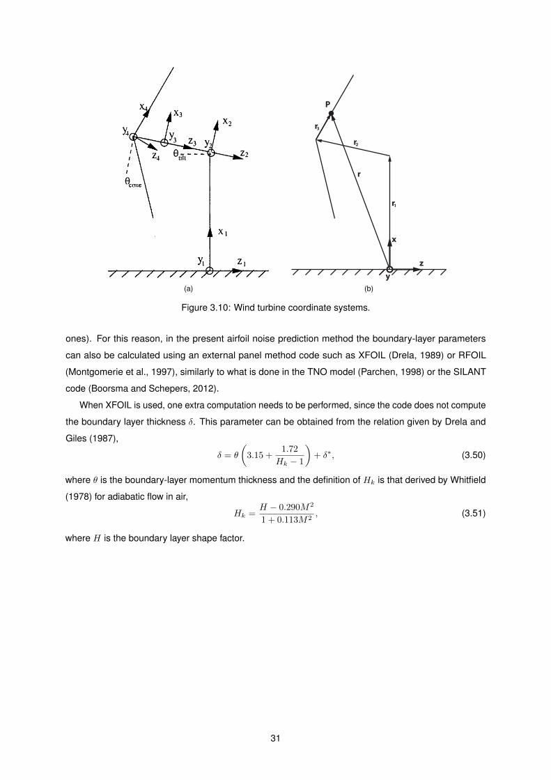
(a)

x

z

y

P

r1

r2

r3

r

(b)

Figure 3.10: Wind turbine coordinate systems.

ones). For this reason, in the present airfoil noise prediction method the boundary-layer parameters

can also be calculated using an external panel method code such as XFOIL (Drela, 1989) or RFOIL

(Montgomerie et al., 1997), similarly to what is done in the TNO model (Parchen, 1998) or the SILANT

code (Boorsma and Schepers, 2012).

When XFOIL is used, one extra computation needs to be performed, since the code does not compute

the boundary layer thickness δ. This parameter can be obtained from the relation given by Drela and

Giles (1987),

δ = θ

(3.15 +

1.72

Hk − 1

)+ δ∗, (3.50)

where θ is the boundary-layer momentum thickness and the definition of Hk is that derived by Whitfield

(1978) for adiabatic flow in air,

Hk =H − 0.290M2

1 + 0.113M2, (3.51)

where H is the boundary layer shape factor.

31

32

Chapter 4

Blade Geometry and Parameterization

In order to analyze a wind turbine, it is necessary to model the geometry of its blades. This model should

have as few input parameters as possible, since the objective of this work is to perform optimization

of the blade geometry. In this work, the geometry is defined by setting the radial distribution of three

independent parameters: twist, chord and airfoil shape. With these distributions, the blade geometry is

generated by the following steps:

1. Connect the airfoil shapes to form the blade basis, with unit chord;

2. Apply the chord distribution to the basis blade, scaling each spanwise station by the local chord

value;

3. Apply the twist distribution, rotating each section about its aerodynamic center (usually at 1/4 chord).

Using this method, the geometry can be easily introduced into the BEM method (where the twist,

chord and airfoil aerodynamic data are separate inputs) or used in a more complex CFD computation,

where, in order to generate the mesh, the full 3D geometry is required. The fact that they are independent

of each other also allows for their separate optimization.

4.1 Twist and Chord distribution

Both the twist and chord distributions are defined by a set of control points which are either linearly

interpolated or used to define a Bezier curve. The degree of the Bezier curve will depend on the number

of control points. Figure 4.1 shows an example of a twist and chord distribution using Bezier curves.

4.2 Airfoil Shape Distribution

The unitary chord, non-twisted shape of the blade is defined by linear interpolation of control cross-

sections airfoils along the blade, which can be defined by their coordinates. As the intent of this work is

to perform optimizations on the blade geometry, this approach is not acceptable, leading to the need to

represent the cross-sections shapes using a smaller number of parameters.

33

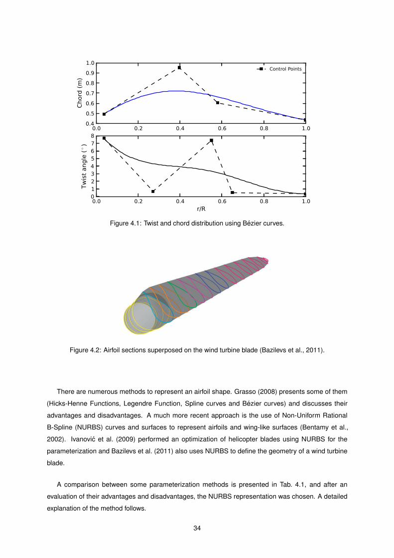
0.0 0.2 0.4 0.6 0.8 1.00.4

0.5

0.6

0.7

0.8

0.9

1.0

Chord (m)

Control Points

0.0 0.2 0.4 0.6 0.8 1.0

r/R

012345678

Twist angle (

◦ )

Figure 4.1: Twist and chord distribution using Bezier curves.

Figure 4.2: Airfoil sections superposed on the wind turbine blade (Bazilevs et al., 2011).

There are numerous methods to represent an airfoil shape. Grasso (2008) presents some of them

(Hicks-Henne Functions, Legendre Function, Spline curves and Bezier curves) and discusses their

advantages and disadvantages. A much more recent approach is the use of Non-Uniform Rational

B-Spline (NURBS) curves and surfaces to represent airfoils and wing-like surfaces (Bentamy et al.,

2002). Ivanovic et al. (2009) performed an optimization of helicopter blades using NURBS for the

parameterization and Bazilevs et al. (2011) also uses NURBS to define the geometry of a wind turbine

blade.

A comparison between some parameterization methods is presented in Tab. 4.1, and after an

evaluation of their advantages and disadvantages, the NURBS representation was chosen. A detailed

explanation of the method follows.

34

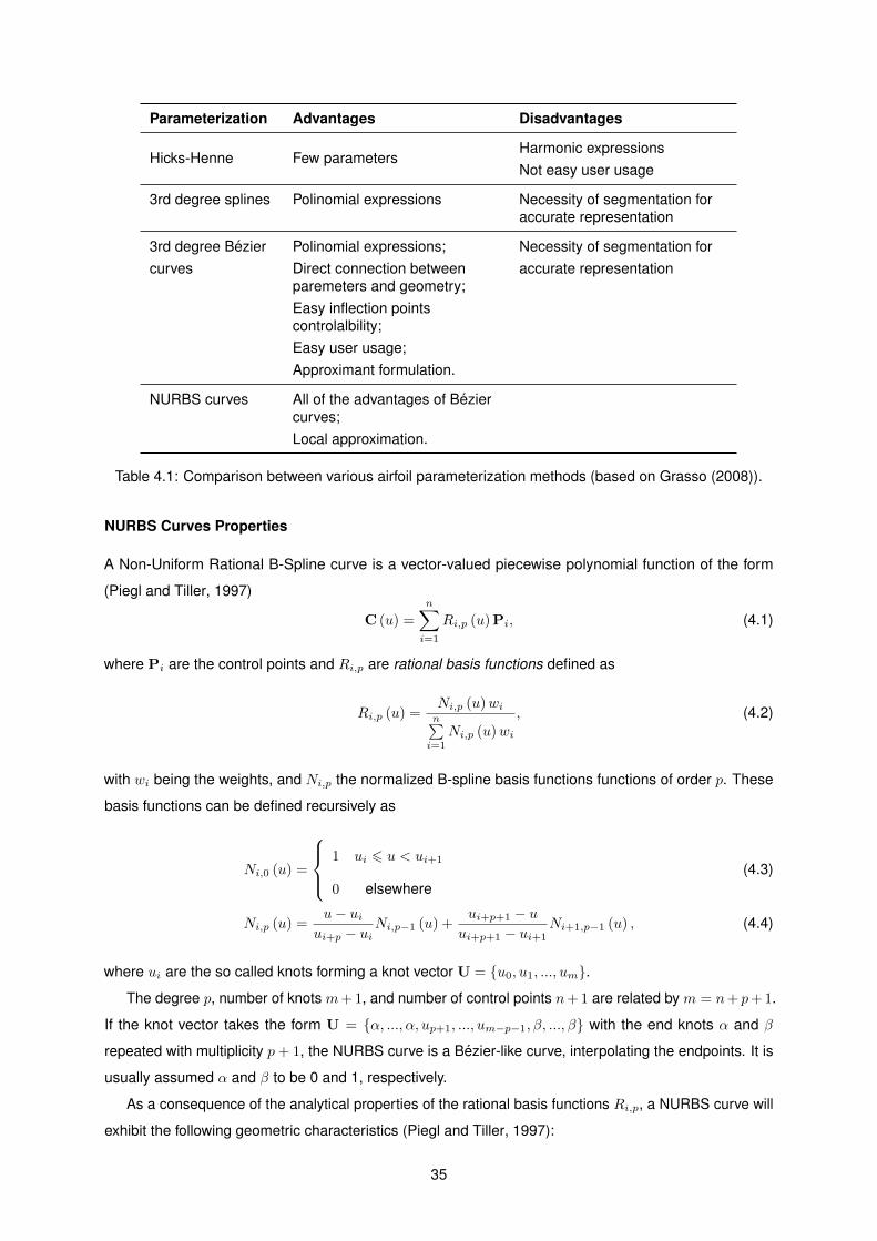
Parameterization Advantages Disadvantages

Hicks-Henne Few parametersHarmonic expressionsNot easy user usage

3rd degree splines Polinomial expressions Necessity of segmentation foraccurate representation

3rd degree Bezier Polinomial expressions; Necessity of segmentation forcurves Direct connection between

paremeters and geometry;accurate representation

Easy inflection pointscontrolalbility;Easy user usage;Approximant formulation.

NURBS curves All of the advantages of Beziercurves;Local approximation.

Table 4.1: Comparison between various airfoil parameterization methods (based on Grasso (2008)).

NURBS Curves Properties

A Non-Uniform Rational B-Spline curve is a vector-valued piecewise polynomial function of the form

(Piegl and Tiller, 1997)

C (u) =

n∑i=1

Ri,p (u)Pi, (4.1)

where Pi are the control points and Ri,p are rational basis functions defined as

Ri,p (u) =Ni,p (u)win∑i=1

Ni,p (u)wi

, (4.2)

with wi being the weights, and Ni,p the normalized B-spline basis functions functions of order p. These

basis functions can be defined recursively as

Ni,0 (u) =

1 ui 6 u < ui+1

0 elsewhere(4.3)

Ni,p (u) =u− ui

ui+p − uiNi,p−1 (u) +

ui+p+1 − uui+p+1 − ui+1

Ni+1,p−1 (u) , (4.4)

where ui are the so called knots forming a knot vector U = {u0, u1, ..., um}.

The degree p, number of knots m+ 1, and number of control points n+ 1 are related by m = n+ p+ 1.

If the knot vector takes the form U = {α, ..., α, up+1, ..., um−p−1, β, ..., β} with the end knots α and β

repeated with multiplicity p+ 1, the NURBS curve is a Bezier-like curve, interpolating the endpoints. It is

usually assumed α and β to be 0 and 1, respectively.

As a consequence of the analytical properties of the rational basis functions Ri,p, a NURBS curve will

exhibit the following geometric characteristics (Piegl and Tiller, 1997):

35

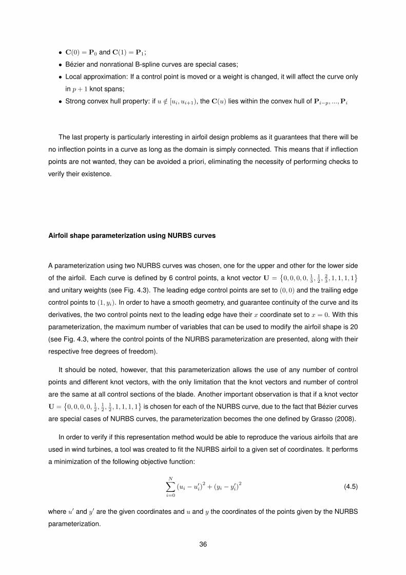
• C(0) = P0 and C(1) = P1;

• Bezier and nonrational B-spline curves are special cases;

• Local approximation: If a control point is moved or a weight is changed, it will affect the curve only

in p+ 1 knot spans;

• Strong convex hull property: if u /∈ [ui, ui+1), the C(u) lies within the convex hull of Pi−p, ...,Pi

The last property is particularly interesting in airfoil design problems as it guarantees that there will be

no inflection points in a curve as long as the domain is simply connected. This means that if inflection

points are not wanted, they can be avoided a priori, eliminating the necessity of performing checks to

verify their existence.

Airfoil shape parameterization using NURBS curves

A parameterization using two NURBS curves was chosen, one for the upper and other for the lower side

of the airfoil. Each curve is defined by 6 control points, a knot vector U ={

0, 0, 0, 0, 13 ,

12 ,

23 , 1, 1, 1, 1

}and unitary weights (see Fig. 4.3). The leading edge control points are set to (0, 0) and the trailing edge

control points to (1, yi). In order to have a smooth geometry, and guarantee continuity of the curve and its

derivatives, the two control points next to the leading edge have their x coordinate set to x = 0. With this

parameterization, the maximum number of variables that can be used to modify the airfoil shape is 20

(see Fig. 4.3, where the control points of the NURBS parameterization are presented, along with their

respective free degrees of freedom).

It should be noted, however, that this parameterization allows the use of any number of control

points and different knot vectors, with the only limitation that the knot vectors and number of control

are the same at all control sections of the blade. Another important observation is that if a knot vector

U ={

0, 0, 0, 0, 12 ,

12 ,

12 , 1, 1, 1, 1

}is chosen for each of the NURBS curve, due to the fact that Bezier curves

are special cases of NURBS curves, the parameterization becomes the one defined by Grasso (2008).

In order to verify if this representation method would be able to reproduce the various airfoils that are

used in wind turbines, a tool was created to fit the NURBS airfoil to a given set of coordinates. It performs

a minimization of the following objective function:

N∑i=0

(ui − u′i)2

+ (yi − y′i)2 (4.5)

where u′ and y′ are the given coordinates and u and y the coordinates of the points given by the NURBS

parameterization.

36

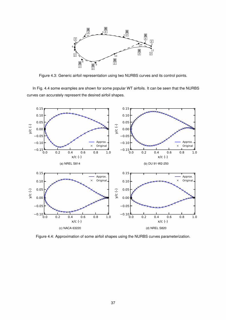
yxy

xyx

yx

yx

yx

yxy

x

y

yy

y

Figure 4.3: Generic airfoil representation using two NURBS curves and its control points.

In Fig. 4.4 some examples are shown for some popular WT airfoils. It can be seen that the NURBS

curves can accurately represent the desired airfoil shapes.

0.0 0.2 0.4 0.6 0.8 1.0

x/c (-)

−0.15

−0.10

−0.05

0.00

0.05

0.10

0.15

y/c

(-)

Approx.

Original

(a) NREL S814

0.0 0.2 0.4 0.6 0.8 1.0

x/c (-)

−0.15

−0.10

−0.05

0.00

0.05

0.10

0.15

y/c

(-)

Approx.

Original

(b) DU 91-W2-250

0.0 0.2 0.4 0.6 0.8 1.0

x/c (-)

−0.10

−0.05

0.00

0.05

0.10

0.15

y/c

(-)

Approx.

Original

(c) NACA 63220

0.0 0.2 0.4 0.6 0.8 1.0

x/c (-)

−0.10

−0.05

0.00

0.05

0.10

0.15

y/c

(-)

Approx.

Original

(d) NREL S820

Figure 4.4: Approximation of some airfoil shapes using the NURBS curves parameterization.

37

38

Chapter 5

Wind Turbine Noise Prediction Code

A wind turbine performance and noise prediction code was developed using the models introduced in the

previous chapters. The code was written in Python and C++, taking both advantage of the speed of the

C++ language and the flexibility of the Python language. In this chapter, the code structure is described,

together with an explanation of the design choices and approaches taken in the development. In the

end of the chapter, the code is validated against experimental data and data obtained using another

simulation tool.

5.1 Code Structure

The code was developed making use of the object-oriented programming capabilities of both the Python

and C++ languages, thus allowing to develop a robust and modular code. This approach allows the

possibility to include different aerodynamic or aeroacoustic prediction models without much effort. The

interface between the two languages is done using SWIG (Beazley, 1996), a software development tool

that connects programs written in C and C++ with a variety of high-level programming languages. By

using this interface, the need of the use of files for transferring data between the codes was eliminated.

The code can be divided into three parts, the geometry definition classes (Rotor, Blade and Section),

the rotor analysis class (Analysis) and the airfoil aerodynamic analysis classes Polar and BLayer. The

Analysis class contains two functions, the aerodynamic and the aeroacoustic analysis functions, which

make use of the BEM and the NOISE C++ libraries, respectively, as well of the Polar and BLayer classes.

A non extensive description of some of the data and functions of each class is given in Tables 5.1 to 5.6

and the interaction between the classes of the code is schematically represented in Fig. 5.1.

5.2 Code Inputs and Output

In this section, the inputs and output of the code are described regarding the geometry of the blade, the

analysis and the aerodynamic polars. Each of the previous can be defined via an input file, but it should

be noted that they can also be defined with a Python script file.

39

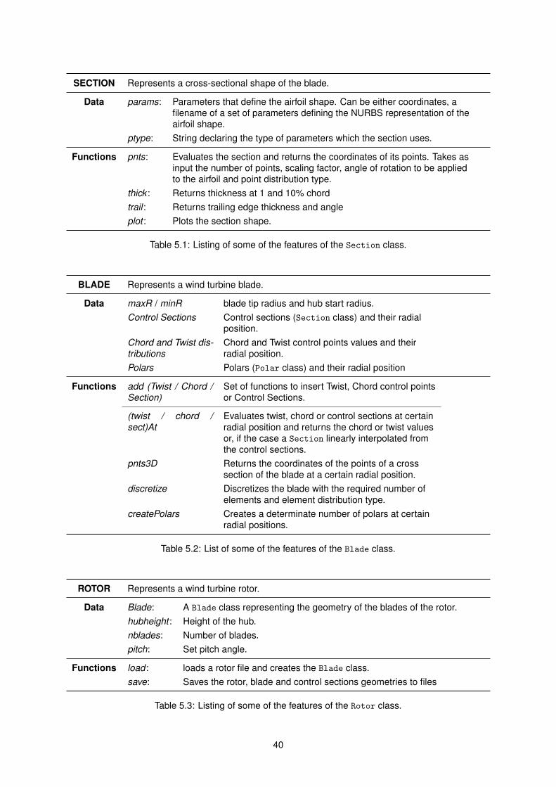
SECTION Represents a cross-sectional shape of the blade.

Data params: Parameters that define the airfoil shape. Can be either coordinates, afilename of a set of parameters defining the NURBS representation of theairfoil shape.

ptype: String declaring the type of parameters which the section uses.

Functions pnts: Evaluates the section and returns the coordinates of its points. Takes asinput the number of points, scaling factor, angle of rotation to be appliedto the airfoil and point distribution type.

thick : Returns thickness at 1 and 10% chordtrail : Returns trailing edge thickness and angleplot : Plots the section shape.

Table 5.1: Listing of some of the features of the Section class.

BLADE Represents a wind turbine blade.

Data maxR / minR blade tip radius and hub start radius.Control Sections Control sections (Section class) and their radial

position.Chord and Twist dis-tributions

Chord and Twist control points values and theirradial position.

Polars Polars (Polar class) and their radial position

Functions add (Twist / Chord /Section)

Set of functions to insert Twist, Chord control pointsor Control Sections.

(twist / chord /sect)At

Evaluates twist, chord or control sections at certainradial position and returns the chord or twist valuesor, if the case a Section linearly interpolated fromthe control sections.

pnts3D Returns the coordinates of the points of a crosssection of the blade at a certain radial position.

discretize Discretizes the blade with the required number ofelements and element distribution type.

createPolars Creates a determinate number of polars at certainradial positions.

Table 5.2: List of some of the features of the Blade class.

ROTOR Represents a wind turbine rotor.

Data Blade: A Blade class representing the geometry of the blades of the rotor.hubheight : Height of the hub.nblades: Number of blades.pitch: Set pitch angle.

Functions load : loads a rotor file and creates the Blade class.save: Saves the rotor, blade and control sections geometries to files

Table 5.3: Listing of some of the features of the Rotor class.

40

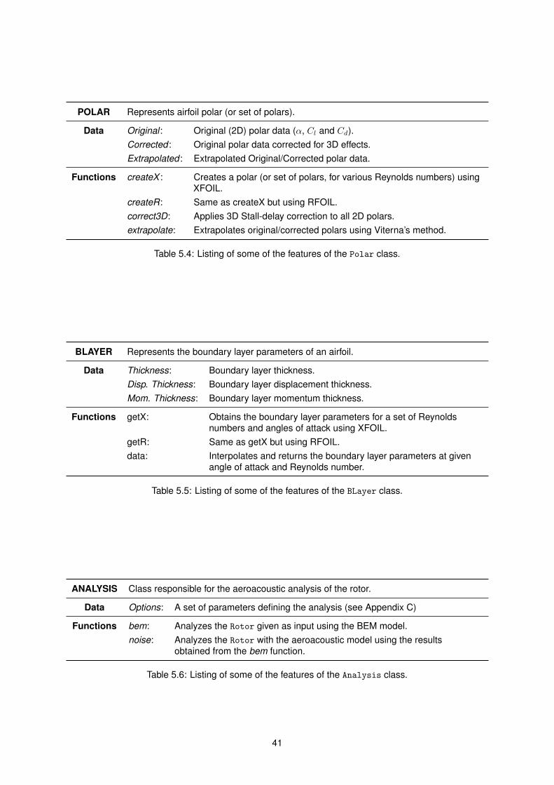
POLAR Represents airfoil polar (or set of polars).

Data Original : Original (2D) polar data (α, Cl and Cd).Corrected : Original polar data corrected for 3D effects.Extrapolated : Extrapolated Original/Corrected polar data.

Functions createX : Creates a polar (or set of polars, for various Reynolds numbers) usingXFOIL.

createR: Same as createX but using RFOIL.correct3D: Applies 3D Stall-delay correction to all 2D polars.extrapolate: Extrapolates original/corrected polars using Viterna’s method.

Table 5.4: Listing of some of the features of the Polar class.

BLAYER Represents the boundary layer parameters of an airfoil.

Data Thickness: Boundary layer thickness.Disp. Thickness: Boundary layer displacement thickness.Mom. Thickness: Boundary layer momentum thickness.

Functions getX: Obtains the boundary layer parameters for a set of Reynoldsnumbers and angles of attack using XFOIL.

getR: Same as getX but using RFOIL.data: Interpolates and returns the boundary layer parameters at given

angle of attack and Reynolds number.

Table 5.5: Listing of some of the features of the BLayer class.

ANALYSIS Class responsible for the aeroacoustic analysis of the rotor.

Data Options: A set of parameters defining the analysis (see Appendix C)

Functions bem: Analyzes the Rotor given as input using the BEM model.noise: Analyzes the Rotor with the aeroacoustic model using the results

obtained from the bem function.

Table 5.6: Listing of some of the features of the Analysis class.

41

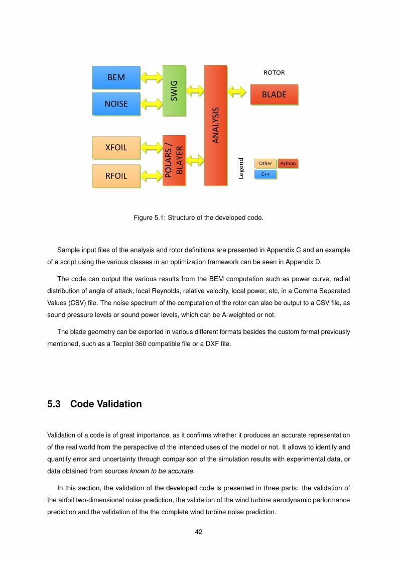
ROTOR

Leg

en

d

BEM

NOISE

SWIG

XFOIL

RFOIL PO

LAR

S /

BLA

YER

AN

ALY

SIS

BLADE

Other Python

C++

Figure 5.1: Structure of the developed code.

Sample input files of the analysis and rotor definitions are presented in Appendix C and an example

of a script using the various classes in an optimization framework can be seen in Appendix D.

The code can output the various results from the BEM computation such as power curve, radial

distribution of angle of attack, local Reynolds, relative velocity, local power, etc, in a Comma Separated

Values (CSV) file. The noise spectrum of the computation of the rotor can also be output to a CSV file, as

sound pressure levels or sound power levels, which can be A-weighted or not.

The blade geometry can be exported in various different formats besides the custom format previously

mentioned, such as a Tecplot 360 compatible file or a DXF file.

5.3 Code Validation

Validation of a code is of great importance, as it confirms whether it produces an accurate representation

of the real world from the perspective of the intended uses of the model or not. It allows to identify and

quantify error and uncertainty through comparison of the simulation results with experimental data, or

data obtained from sources known to be accurate.

In this section, the validation of the developed code is presented in three parts: the validation of

the airfoil two-dimensional noise prediction, the validation of the wind turbine aerodynamic performance

prediction and the validation of the the complete wind turbine noise prediction.

42

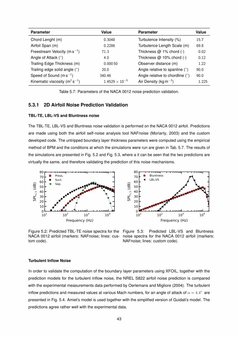
Parameter Value Parameter Value

Chord Lenght (m) 0.3048 Turbulence Intensity (%) 15.7

Airfoil Span (m) 0.2286 Turbulence Length Scale (m) 69.8

Freestream Velocity (m s−1) 71.3 Thickness @ 1% chord (-) 0.02

Angle of Attack (◦) 4.0 Thickness @ 10% chord (-) 0.12

Trailing Edge Thickness (m) 0.000 50 Observer distance (m) 1.22

Trailing edge solid angle (◦) 20.0 Angle relative to spanline (◦) 90.0

Speed of Sound (m s−1) 340.46 Angle relative to chordline (◦) 90.0

Kinematic viscosity (m2 s−1) 1.4529× 10−5 Air Density (kg m−3) 1.225

Table 5.7: Parameters of the NACA 0012 noise prediction validation.

5.3.1 2D Airfoil Noise Prediction Validation

TBL-TE, LBL-VS and Bluntness noise

The TBL-TE, LBL-VS and Bluntness noise validation is performed on the NACA 0012 airfoil. Predictions

are made using both the airfoil self-noise analysis tool NAFnoise (Moriarty, 2003) and the custom

developed code. The untripped boundary layer thickness parameters were computed using the empirical

method of BPM and the conditions at which the simulations were run are given in Tab. 5.7. The results of

the simulations are presented in Fig. 5.2 and Fig. 5.3, where a it can be seen that the two predictions are

virtually the same, and therefore validating the prediction of this noise mechanisms.

101 102 103 104

Frequency (Hz)

0

10

20

30

40

50

60

70

80

SPL 1

/3 (dB)

Press.

Suct.

Sep.

Figure 5.2: Predicted TBL-TE noise spectra for theNACA 0012 airfoil (markers: NAFnoise; lines: cus-tom code).

101 102 103 104

Frequency (Hz)

0

10

20

30

40

50

60

70

80

SPL 1

/3 (dB)

Bluntness

LBL-VS

Figure 5.3: Predicted LBL-VS and Bluntnessnoise spectra for the NACA 0012 airfoil (markers:NAFnoise; lines: custom code).

Turbulent Inflow Noise

In order to validate the computation of the boundary layer parameters using XFOIL, together with the

prediction models for the turbulent inflow noise, the NREL S822 airfoil noise prediction is compared

with the experimental measurements data performed by Oerlemans and Migliore (2004). The turbulent

inflow predictions and measured values at various Mach numbers, for an angle of attack of α = 4.4◦ are

presented in Fig. 5.4. Amiet’s model is used together with the simplified version of Guidati’s model. The

predictions agree rather well with the experimental data.

43

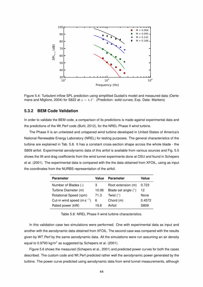
102 103 104

Frequency (Hz)

30

40

50

60

70

80

90

100

SPL 1

/3 (dB)

M = 0.066

M = 0.095

M = 0.141

M = 0.186

Figure 5.4: Turbulent inflow SPL prediction using simplified Guidati’s model and measured data (Oerle-mans and Migliore, 2004) for S822 at α = 4.4◦ . (Prediction: solid curves; Exp. Data: Markers)

5.3.2 BEM Code Validation

In order to validate the BEM code, a comparison of its predictions is made against experimental data and

the predictions of the Wt Perf code (Buhl, 2012), for the NREL Phase II wind turbine.

The Phase II is an untwisted and untapered wind turbine developed in United States of America’s

National Renewable Energy Laboratory (NREL) for testing purposes. The general characteristics of the

turbine are explained in Tab. 5.8. It has a constant cross-section shape across the whole blade - the

S809 airfoil. Experimental aerodynamic data of this airfoil is available from various sources and Fig. 5.5

shows the lift and drag coefficients from the wind tunnel experiments done at OSU and found in Schepers

et al. (2001). The experimental data is compared with the the data obtained from XFOIL, using as input

the coordinates from the NURBS representation of the airfoil.

Parameter Value Parameter Value

Number of Blades (-) 3 Root extension (m) 0.723Turbine Diameter (m) 10.06 Blade set angle (◦) 12Rotational Speed (rpm) 71.3 Twist (◦) NoneCut-in wind speed (m s−1) 6 Chord (m) 0.4572Rated power (kW) 19.8 Airfoil S809

Table 5.8: NREL Phase II wind turbine characteristics.

In this validation case two simulations were performed. One with experimental data as input and

another with the aerodynamic data obtained from XFOIL. The second case was compared with the results

given by WT Perf by the same aerodynamic data. All the simulations were run assuming an air density

equal to 0.9793 kg/m3 as suggested by Schepers et al. (2001).

Figure 5.6 shows the measured (Schepers et al., 2001) and predicted power curves for both the cases

described. The custom code and Wt Perf predicted rather well the aerodynamic power generated by the

turbine. The power curve predicted using aerodynamic data from wind tunnel measurements, although

44

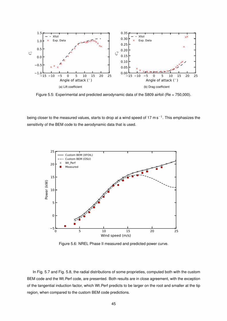
−15 −10 −5 0 5 10 15 20 25

Angle of attack ( ◦ )

−1.0

−0.5

0.0

0.5

1.0

1.5C

l

Xfoil

Exp. Data

(a) Lift coefficient

−15 −10 −5 0 5 10 15 20 25

Angle of attack ( ◦ )

0.00

0.05

0.10

0.15

0.20

0.25

0.30

0.35

Cd

Xfoil

Exp. Data

(b) Drag coefficient

Figure 5.5: Experimental and predicted aerodynamic data of the S809 airfoil (Re = 750,000).

being closer to the measured values, starts to drop at a wind speed of 17 m s−1. This emphasizes the

sensitivity of the BEM code to the aerodynamic data that is used.

0 5 10 15 20 25

Wind speed (m/s)

−5

0

5

10

15

20

25

Pow

er

(kW

)

Custom BEM (XFOIL)

Custom BEM (OSU)

Wt_Perf

Measured

Figure 5.6: NREL Phase II measured and predicted power curve.

In Fig. 5.7 and Fig. 5.8, the radial distributions of some proprieties, computed both with the custom

BEM code and the Wt Perf code, are presented. Both results are in close agreement, with the exception

of the tangential induction factor, which Wt Perf predicts to be larger on the root and smaller at the tip

region, when compared to the custom BEM code predictions.

45

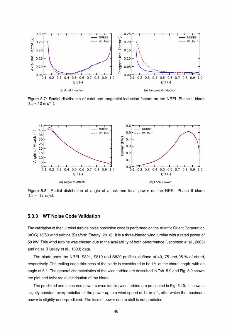
0.1 0.2 0.3 0.4 0.5 0.6 0.7 0.8 0.9 1.0

r/R (-)

0.05

0.10

0.15

0.20

0.25

0.30A

xia

l In

d.

Fact

or

(-) NURBS

Wt_Perf

(a) Axial Induction

0.1 0.2 0.3 0.4 0.5 0.6 0.7 0.8 0.9 1.0

r/R (-)

0.00

0.05

0.10

0.15

0.20

0.25

Tangent. Ind. Factor (-)

NURBS

Wt_Perf

(b) Tangential Induction

Figure 5.7: Radial distribution of axial and tangential induction factors on the NREL Phase II blade(U0 = 12 m s−1).

0.1 0.2 0.3 0.4 0.5 0.6 0.7 0.8 0.9 1.0

r/R (-)

0

510

1520

25

30

35

40

45

Angle of Attack (

◦ )

NURBS

Wt_Perf

(a) Angle of Attack

0.1 0.2 0.3 0.4 0.5 0.6 0.7 0.8 0.9 1.0

r/R (-)

0.0

0.1

0.2

0.3

0.4

0.5

0.6Po

wer (kW)

NURBS

Wt_Perf

(b) Local Power

Figure 5.8: Radial distribution of angle of attack and local power on the NREL Phase II blade(U0 = 12 m/s).

5.3.3 WT Noise Code Validation

The validation of the full wind turbine noise prediction code is performed on the Atlantic Orient Corporation

(AOC) 15/50 wind turbine (Seaforth Energy, 2010). It is a three-bladed wind turbine with a rated power of

50 kW. This wind turbine was chosen due to the availability of both performance (Jacobson et al., 2003)

and noise (Huskey et al., 1999) data.

The blade uses the NREL S821, S819 and S820 profiles, defined at 40, 75 and 95 % of chord,

respectively. The trailing edge thickness of the blade is considered to be 1% of the chord length, with an

angle of 6 ◦. The general characteristics of the wind turbine are described in Tab. 5.9 and Fig. 5.9 shows

the plot and twist radial distribution of the blade.

The predicted and measured power curves for this wind turbine are presented in Fig. 5.10. It shows a

slightly constant overprediction of the power up to a wind speed of 14 m s−1, after which the maximum

power is slightly underpredicted. The loss of power due to stall is not predicted.

46

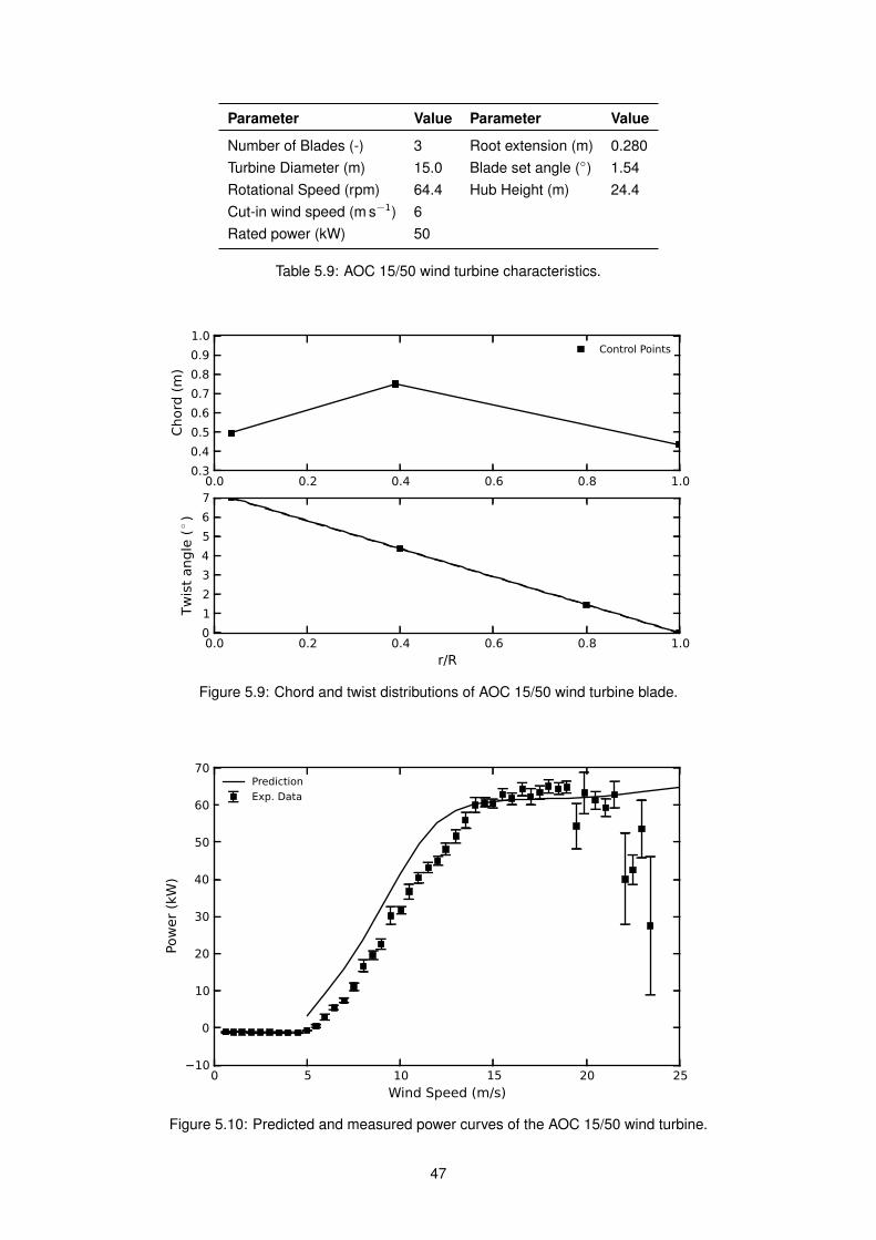
Parameter Value Parameter Value

Number of Blades (-) 3 Root extension (m) 0.280Turbine Diameter (m) 15.0 Blade set angle (◦) 1.54Rotational Speed (rpm) 64.4 Hub Height (m) 24.4Cut-in wind speed (m s−1) 6Rated power (kW) 50

Table 5.9: AOC 15/50 wind turbine characteristics.

0.0 0.2 0.4 0.6 0.8 1.00.3

0.4

0.5

0.6

0.7

0.8

0.9

1.0

Chord (m)

Control Points

0.0 0.2 0.4 0.6 0.8 1.0

r/R

0

1

2

3

4

5

6

7

Twist angle (

◦ )

Figure 5.9: Chord and twist distributions of AOC 15/50 wind turbine blade.

0 5 10 15 20 25

Wind Speed (m/s)

−10

0

10

20

30

40

50

60

70

Pow

er

(kW

)

Prediction

Exp. Data

Figure 5.10: Predicted and measured power curves of the AOC 15/50 wind turbine.

47

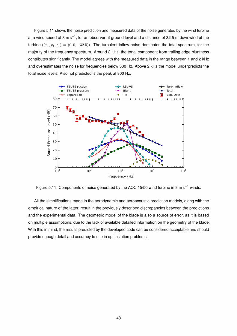
Figure 5.11 shows the noise prediction and measured data of the noise generated by the wind turbine

at a wind speed of 8 m s−1, for an observer at ground level and a distance of 32.5 m downwind of the

turbine ((x1, y1, z1) = (0, 0,−32.5)). The turbulent inflow noise dominates the total spectrum, for the

majority of the frequency spectrum. Around 2 kHz, the tonal component from trailing edge bluntness

contributes significantly. The model agrees with the measured data in the range between 1 and 2 kHz

and overestimates the noise for frequencies below 500 Hz. Above 2 kHz the model underpredicts the

total noise levels. Also not predicted is the peak at 800 Hz.

101 102 103 104 105

Frequency (Hz)

0

10

20

30

40

50

60

70

80

So

un

d P

ress

ure

Le

ve

l (d

B)

TBL-TE suction

TBL-TE pressure

Separation

LBL-VS

Blunt

Tip

Turb. Inflow

Total

Exp. Data

Figure 5.11: Components of noise generated by the AOC 15/50 wind turbine in 8 m s−1 winds.

All the simplifications made in the aerodynamic and aeroacoustic prediction models, along with the

empirical nature of the latter, result in the previously described discrepancies between the predictions

and the experimental data. The geometric model of the blade is also a source of error, as it is based

on multiple assumptions, due to the lack of available detailed information on the geometry of the blade.

With this in mind, the results predicted by the developed code can be considered acceptable and should

provide enough detail and accuracy to use in optimization problems.

48

Chapter 6

Optimization Framework

Every optimization problem aims to optimize an objective function (either by minimizing or maximizing

its value) which is a function of a set of design variables and is subject to a series of constraints.

Mathematically, the problem takes the form

minimize f(x)

subject to gi(x) 6 0, i = 1, . . . ,m

hj(x) = 0, j = 1, . . . , n

xLk < xk < xUk , k = 1, . . . , p

(6.1)

where x is a vector containing the design variables xi, ..., xp, f(x) is the objective function, and gi(x) and

hj(x) are the inequality and equality constraints, respectively. Each variable is bounded by its lower and

upper limits xLk and xUk , referred to as side constraints. The design space region in where the variables

satisfy all equality, inequality and side constrains is called the feasible search region. For a more detailed

definition of the optimization problem and insight on the subject of numerical optimization, the reader

should refer to the available literature (Bonnans et al., 2006; Pedregal, 2003).

In this chapter, the optimization framework developed is presented. First the numerical optimization

algorithms used in this work are introduced, followed by the description of the framework structure.

The chapter ends with convergence analysis of the selected optimization algorithm as a function of the

optimization parameters.

6.1 Numerical Optimization Methods

The optimization field has been growing rapidly for the past few decades, with many new theoretical,

algorithmic and computational contributions to solve various problems. Optimization methods can be

divided in two main different approaches: deterministic and heuristic (see Fig. 6.1). Deterministic methods

take advantage of the analytical properties of the problem to generate a sequence of points that converge

to a local optimal solution. Examples of deterministic methods are Linear Programming, Nonlinear

49

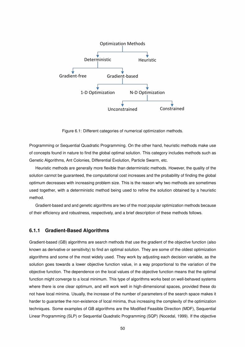
Deterministic Heuristic

Gradient-free Gradient-based

1-D Optimization N-D Optimization

Unconstrained Constrained

Optimization Methods

Figure 6.1: Different categories of numerical optimization methods.

Programming or Sequential Quadratic Programming. On the other hand, heuristic methods make use

of concepts found in nature to find the global optimal solution. This category includes methods such as

Genetic Algorithms, Ant Colonies, Differential Evolution, Particle Swarm, etc.

Heuristic methods are generally more flexible than deterministic methods. However, the quality of the

solution cannot be guaranteed, the computational cost increases and the probability of finding the global

optimum decreases with increasing problem size. This is the reason why two methods are sometimes

used together, with a deterministic method being used to refine the solution obtained by a heuristic

method.

Gradient-based and and genetic algorithms are two of the most popular optimization methods because

of their efficiency and robustness, respectively, and a brief description of these methods follows.

6.1.1 Gradient-Based Algorithms

Gradient-based (GB) algorithms are search methods that use the gradient of the objective function (also

known as derivative or sensitivity) to find an optimal solution. They are some of the oldest optimization

algorithms and some of the most widely used. They work by adjusting each decision variable, as the

solution goes towards a lower objective function value, in a way proportional to the variation of the

objective function. The dependence on the local values of the objective function means that the optimal

function might converge to a local minimum. This type of algorithms works best on well-behaved systems

where there is one clear optimum, and will work well in high-dimensional spaces, provided these do

not have local minima. Usually, the increase of the number of parameters of the search space makes it

harder to guarantee the non-existence of local minima, thus increasing the complexity of the optimization

techniques. Some examples of GB algorithms are the Modified Feasible Direction (MDF), Sequential

Linear Programming (SLP) or Sequential Quadratic Programming (SQP) (Nocedal, 1999). If the objective

50

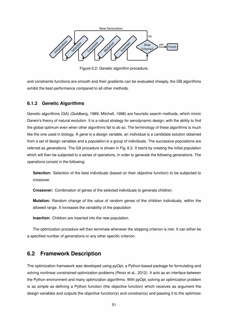
Initi

aliza

tion

Sele

ctio

n

Cross

over

Muta

tion

Inse

rtion Stop

Criteria?

New Generation

no

yesFinish

Figure 6.2: Genetic algorithm procedure.

and constraints functions are smooth and their gradients can be evaluated cheaply, the GB algorithms

exhibit the best performance compared to all other methods.

6.1.2 Genetic Algorithms

Genetic algorithms (GA) (Goldberg, 1989; Mitchell, 1998) are heuristic search methods, which mimic

Darwin’s theory of natural evolution. It is a robust strategy for aerodynamic design, with the ability to find

the global optimum even when other algorithms fail to do so. The terminology of these algorithms is much

like the one used in biology. A gene is a design variable, an individual is a candidate solution obtained

from a set of design variables and a population is a group of individuals. The successive populations are

referred as generations. The GA procedure is shown in Fig. 6.2. It starts by creating the initial population

which will then be subjected to a series of operations, in order to generate the following generations. The

operations consist in the following:

Selection: Selection of the best individuals (based on their objective function) to be subjected to

crossover.

Crossover: Combination of genes of the selected individuals to generate children.

Mutation: Random change of the value of random genes of the children individuals, within the

allowed range. It increases the variability of the population

Insertion: Children are inserted into the new population.

The optimization procedure will then terminate whenever the stopping criterion is met. It can either be

a specified number of generations or any other specific criterion.

6.2 Framework Description

The optimization framework was developed using pyOpt, a Python-based package for formulating and

solving nonlinear constrained optimization problems (Perez et al., 2012). It acts as an interface between

the Python environment and many optimization algorithms. With pyOpt, solving an optimization problem

is as simple as defining a Python function (the objective function) which receives as argument the

design variables and outputs the objective function(s) and constrain(s) and passing it to the optimizer.

51

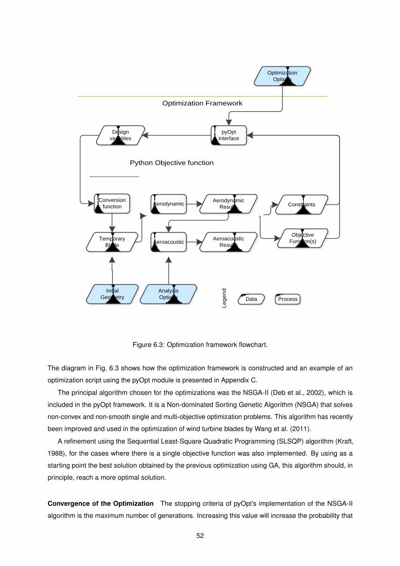
Optimization Framework

Python Objective function

2. Analysis 3. Results1. Conversion

Le

ge

nd

Conversion

function

Design

variables

Initial

Geometry

Temporary

Blade

Analysis

Options

AerodynamicAerodynamic

Results

AeroacousticAeroacoustic

Results

Constraints

Objective

Function(s)

pyOpt

interface

Optimization

Options

Data Process

Figure 6.3: Optimization framework flowchart.

The diagram in Fig. 6.3 shows how the optimization framework is constructed and an example of an

optimization script using the pyOpt module is presented in Appendix C.

The principal algorithm chosen for the optimizations was the NSGA-II (Deb et al., 2002), which is

included in the pyOpt framework. It is a Non-dominated Sorting Genetic Algorithm (NSGA) that solves

non-convex and non-smooth single and multi-objective optimization problems. This algorithm has recently

been improved and used in the optimization of wind turbine blades by Wang et al. (2011).

A refinement using the Sequential Least-Square Quadratic Programming (SLSQP) algorithm (Kraft,

1988), for the cases where there is a single objective function was also implemented. By using as a

starting point the best solution obtained by the previous optimization using GA, this algorithm should, in

principle, reach a more optimal solution.

Convergence of the Optimization The stopping criteria of pyOpt’s implementation of the NSGA-II

algorithm is the maximum number of generations. Increasing this value will increase the probability that

52

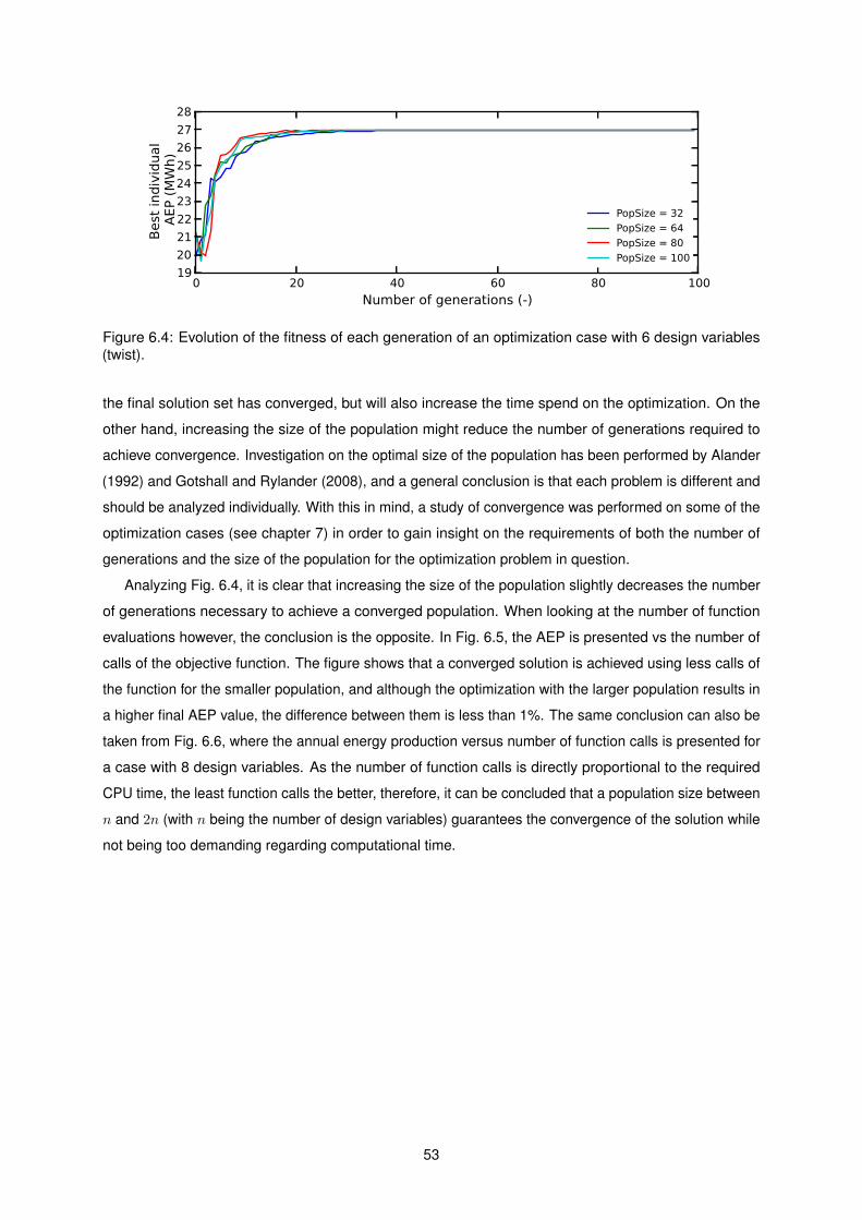
0 20 40 60 80 100

Number of generations (-)

19

20

21

22

23

24

25

26

27

28

Best individual

AEP (MWh)

PopSize = 32

PopSize = 64

PopSize = 80

PopSize = 100

Figure 6.4: Evolution of the fitness of each generation of an optimization case with 6 design variables(twist).

the final solution set has converged, but will also increase the time spend on the optimization. On the

other hand, increasing the size of the population might reduce the number of generations required to

achieve convergence. Investigation on the optimal size of the population has been performed by Alander

(1992) and Gotshall and Rylander (2008), and a general conclusion is that each problem is different and

should be analyzed individually. With this in mind, a study of convergence was performed on some of the

optimization cases (see chapter 7) in order to gain insight on the requirements of both the number of

generations and the size of the population for the optimization problem in question.

Analyzing Fig. 6.4, it is clear that increasing the size of the population slightly decreases the number

of generations necessary to achieve a converged population. When looking at the number of function

evaluations however, the conclusion is the opposite. In Fig. 6.5, the AEP is presented vs the number of

calls of the objective function. The figure shows that a converged solution is achieved using less calls of

the function for the smaller population, and although the optimization with the larger population results in

a higher final AEP value, the difference between them is less than 1%. The same conclusion can also be

taken from Fig. 6.6, where the annual energy production versus number of function calls is presented for

a case with 8 design variables. As the number of function calls is directly proportional to the required

CPU time, the least function calls the better, therefore, it can be concluded that a population size between

n and 2n (with n being the number of design variables) guarantees the convergence of the solution while

not being too demanding regarding computational time.

53

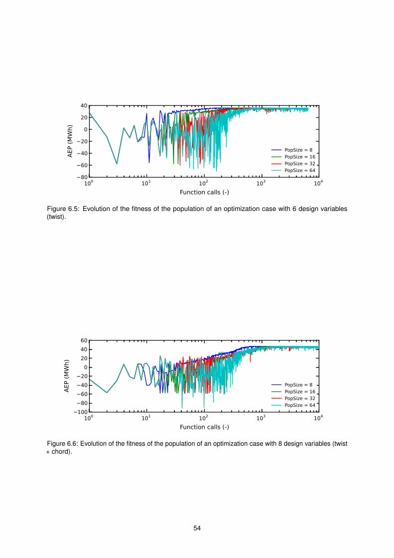
100 101 102 103 104

Function calls (-)

−80

−60

−40

−20

0

20

40

AEP (

MW

h)

PopSize = 8

PopSize = 16

PopSize = 32

PopSize = 64

Figure 6.5: Evolution of the fitness of the population of an optimization case with 6 design variables(twist).

100 101 102 103 104

Function calls (-)

−100

−80

−60

−40

−20

0

20

40

60

AEP (

MW

h)

PopSize = 8

PopSize = 16

PopSize = 32

PopSize = 64

Figure 6.6: Evolution of the fitness of the population of an optimization case with 8 design variables (twist+ chord).

54

Chapter 7

Optimization Results

After introducing all the theory behind the wind turbine aeroacoustic prediction model and the optimization

framework, the most relevant results of the various optimization cases that were run are presented. The

approach for this work was to start with simple optimization problems, such as single objective optimization

on just a few design variables, and gradually increase the number of variables, as well as increasing

the number of objective functions to two. The final optimization problems would be multi-objective

optimizations of both the airfoil shape and chord and twist distribution.

All the optimizations were performed assuming a wind distribution represented by a Weibull curve with

the parameters A and k of 6.48 m s−1 and 1.99, respectively, corresponding to an average wind speed of

6.11 m s−1. These parameters represent the wind distribution in the Portuguese municipality of Vila do

Bispo, in the southwest of Portugal (Costa, 2004).

The performance of the turbine was predicted for a wind speed range from 4 to 25 m s−1, in 1 m s−1

intervals. Due to this, the noise was predicted for a wind speed of 6 m s−1, as it is the closest to the

average wind speed of the selected site. A ground roughness value of 0.08 m was chosen and the

properties assumed for the air are presented in Tab. 7.1 (assuming standard atmosphere conditions at

sea level (McCormick, 1994)). The observer was considered to be located at ground level, at a distance

of 32.5 m downwind of the turbine ((x1, y1, z1) = (0, 0,−32.5)).

Density Kinetic viscosity Speed of sound

1.225 kg m−3 1.46e-5 m2 s−1 340.4 m s−1

Table 7.1: Properties of the air used in the optimizations.

The boundary layer parameters were computed using XFOIL. It as chosen over RFOIL due to the

impossibility of turning off the graphical output of RFOIL, which increased significantly the duration of

each simulation and therefore the optimization.

55

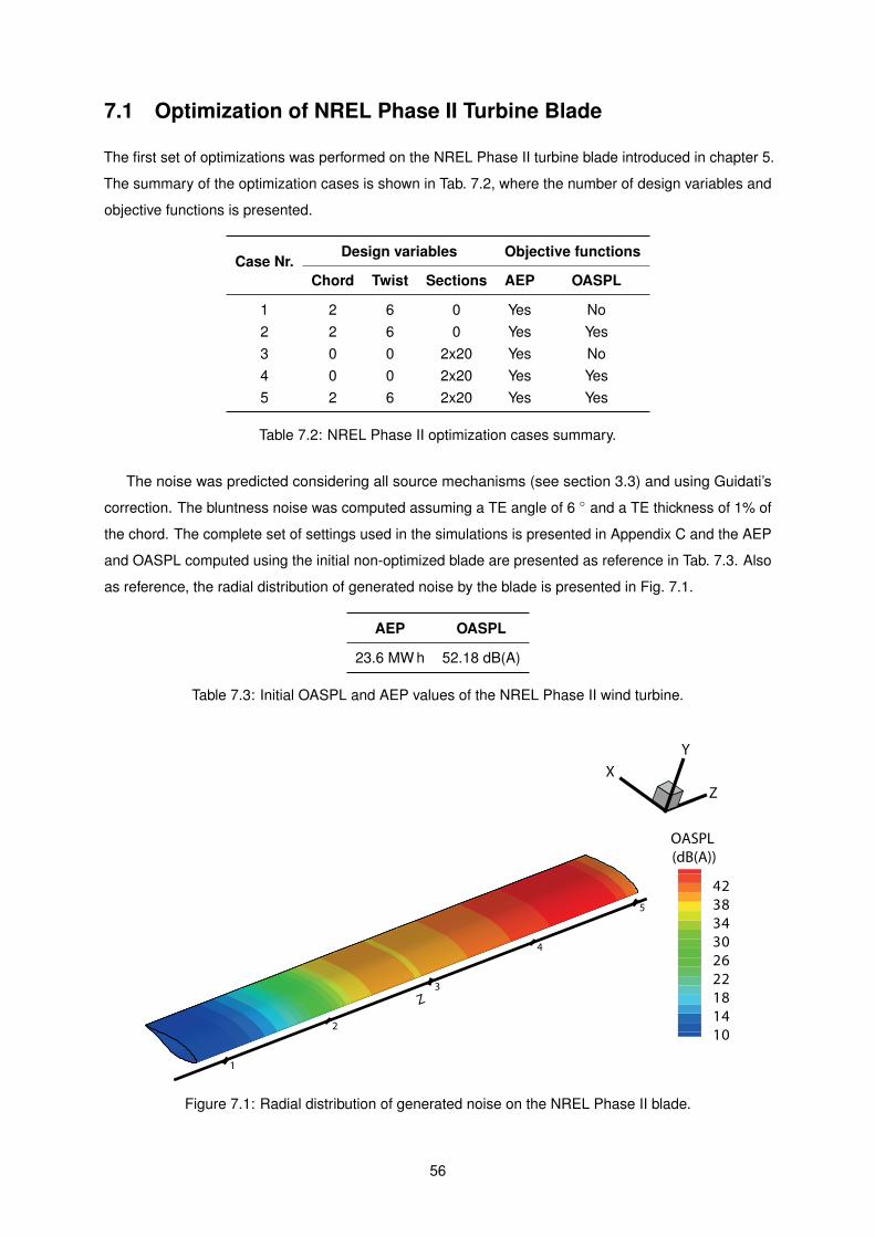
7.1 Optimization of NREL Phase II Turbine Blade

The first set of optimizations was performed on the NREL Phase II turbine blade introduced in chapter 5.

The summary of the optimization cases is shown in Tab. 7.2, where the number of design variables and

objective functions is presented.

Case Nr.Design variables Objective functions

Chord Twist Sections AEP OASPL

1 2 6 0 Yes No2 2 6 0 Yes Yes3 0 0 2x20 Yes No4 0 0 2x20 Yes Yes5 2 6 2x20 Yes Yes

Table 7.2: NREL Phase II optimization cases summary.

The noise was predicted considering all source mechanisms (see section 3.3) and using Guidati’s

correction. The bluntness noise was computed assuming a TE angle of 6 ◦ and a TE thickness of 1% of

the chord. The complete set of settings used in the simulations is presented in Appendix C and the AEP

and OASPL computed using the initial non-optimized blade are presented as reference in Tab. 7.3. Also

as reference, the radial distribution of generated noise by the blade is presented in Fig. 7.1.

AEP OASPL

23.6 MW h 52.18 dB(A)

Table 7.3: Initial OASPL and AEP values of the NREL Phase II wind turbine.

Z

1

2

3

4

5

Z

X

Y

OASPL

(dB(A))

42

38

34

30

26

22

18

14

10

Figure 7.1: Radial distribution of generated noise on the NREL Phase II blade.

56

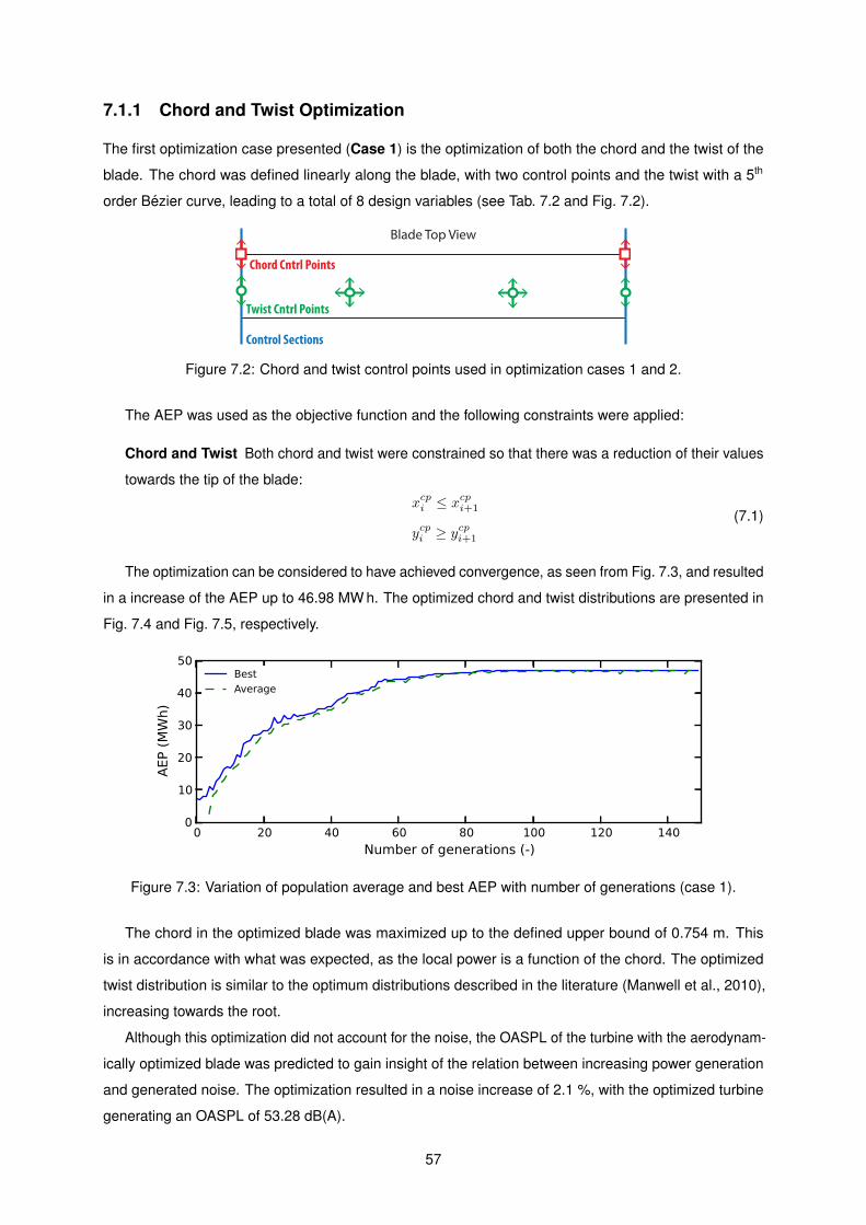
7.1.1 Chord and Twist Optimization

The first optimization case presented (Case 1) is the optimization of both the chord and the twist of the

blade. The chord was defined linearly along the blade, with two control points and the twist with a 5th

order Bezier curve, leading to a total of 8 design variables (see Tab. 7.2 and Fig. 7.2).

Control Sections

Chord Cntrl Points

Twist Cntrl Points

Blade Top View

Figure 7.2: Chord and twist control points used in optimization cases 1 and 2.

The AEP was used as the objective function and the following constraints were applied:

Chord and Twist Both chord and twist were constrained so that there was a reduction of their values

towards the tip of the blade:

xcpi ≤ xcpi+1

ycpi ≥ ycpi+1

(7.1)

The optimization can be considered to have achieved convergence, as seen from Fig. 7.3, and resulted

in a increase of the AEP up to 46.98 MW h. The optimized chord and twist distributions are presented in

Fig. 7.4 and Fig. 7.5, respectively.

0 20 40 60 80 100 120 140

Number of generations (-)

0

10

20

30

40

50

AEP (MWh)

Best

Average

Figure 7.3: Variation of population average and best AEP with number of generations (case 1).

The chord in the optimized blade was maximized up to the defined upper bound of 0.754 m. This

is in accordance with what was expected, as the local power is a function of the chord. The optimized

twist distribution is similar to the optimum distributions described in the literature (Manwell et al., 2010),

increasing towards the root.

Although this optimization did not account for the noise, the OASPL of the turbine with the aerodynam-

ically optimized blade was predicted to gain insight of the relation between increasing power generation

and generated noise. The optimization resulted in a noise increase of 2.1 %, with the optimized turbine

generating an OASPL of 53.28 dB(A).

57

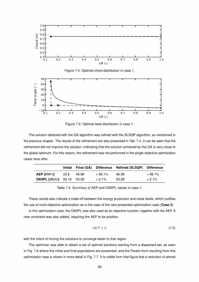
0.1 0.2 0.3 0.4 0.5 0.6 0.7 0.8 0.9 1.0

r/R (-)

0.3

0.4

0.5

0.6

0.7

0.8

0.9

1.0

Chord (m)

Figure 7.4: Optimal chord distribution in case 1.

0.1 0.2 0.3 0.4 0.5 0.6 0.7 0.8 0.9 1.0

r/R (-)

−10

0

10

20

30

40

50

Tw

ist

angle

(◦ )

Figure 7.5: Optimal twist distribution in case 1.

The solution obtained with the GA algorithm was refined with the SLSQP algorithm, as mentioned in

the previous chapter. The results of the refinement are also presented in Tab. 7.4. It can be seen that the

refinement did not improve the solution, indicating that the solution achieved by the GA is very close to

the global optimum. For this reason, the refinement was not performed in the single objective optimization

cases here after.

Initial Final (GA) Difference Refined (SLSQP) Difference

AEP [MW h] 23.6 46.98 + 99.1% 46.98 + 99.1%OASPL [dB(A)] 52.18 53.28 + 2.1% 53.28 + 2.1%

Table 7.4: Summary of AEP and OASPL values in case 1.

These results also indicate a trade-off between the energy production and noise levels, which justifies

the use of multi-objective optimization as is the case of the next presented optimization case (Case 2).

In this optimization case, the OASPL was also used as an objective function, together with the AEP. A

new constraint was also added, requiring the AEP to be positive,

AEP ≥ 0. (7.2)

with the intent of forcing the solutions to converge faster to that region.

The optimizer was able to obtain a set of optimal solutions starting from a dispersed set, as seen

in Fig. 7.6 where the initial and final populations are presented, and the Pareto front resulting from this

optimization case is shown in more detail in Fig. 7.7. It is visible from that figure that a reduction of almost

58

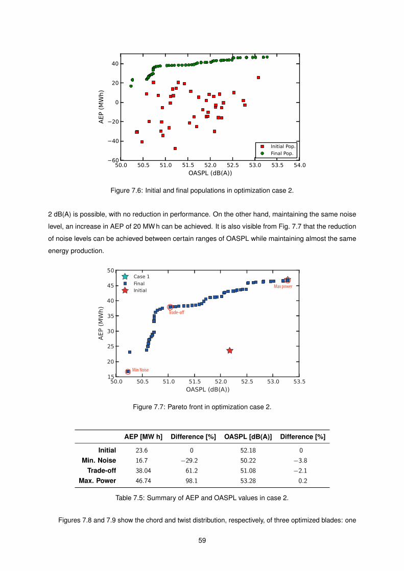
50.0 50.5 51.0 51.5 52.0 52.5 53.0 53.5 54.0

OASPL (dB(A))

−60

−40

−20

0

20

40

AEP (

MW

h)

Initial Pop.

Final Pop.

Figure 7.6: Initial and final populations in optimization case 2.

2 dB(A) is possible, with no reduction in performance. On the other hand, maintaining the same noise

level, an increase in AEP of 20 MW h can be achieved. It is also visible from Fig. 7.7 that the reduction

of noise levels can be achieved between certain ranges of OASPL while maintaining almost the same

energy production.

Min Noise

Max power

Trade-o!

Figure 7.7: Pareto front in optimization case 2.

AEP [MW h] Difference [%] OASPL [dB(A)] Difference [%]

Initial 23.6 0 52.18 0

Min. Noise 16.7 −29.2 50.22 −3.8Trade-off 38.04 61.2 51.08 −2.1

Max. Power 46.74 98.1 53.28 0.2

Table 7.5: Summary of AEP and OASPL values in case 2.

Figures 7.8 and 7.9 show the chord and twist distribution, respectively, of three optimized blades: one

59

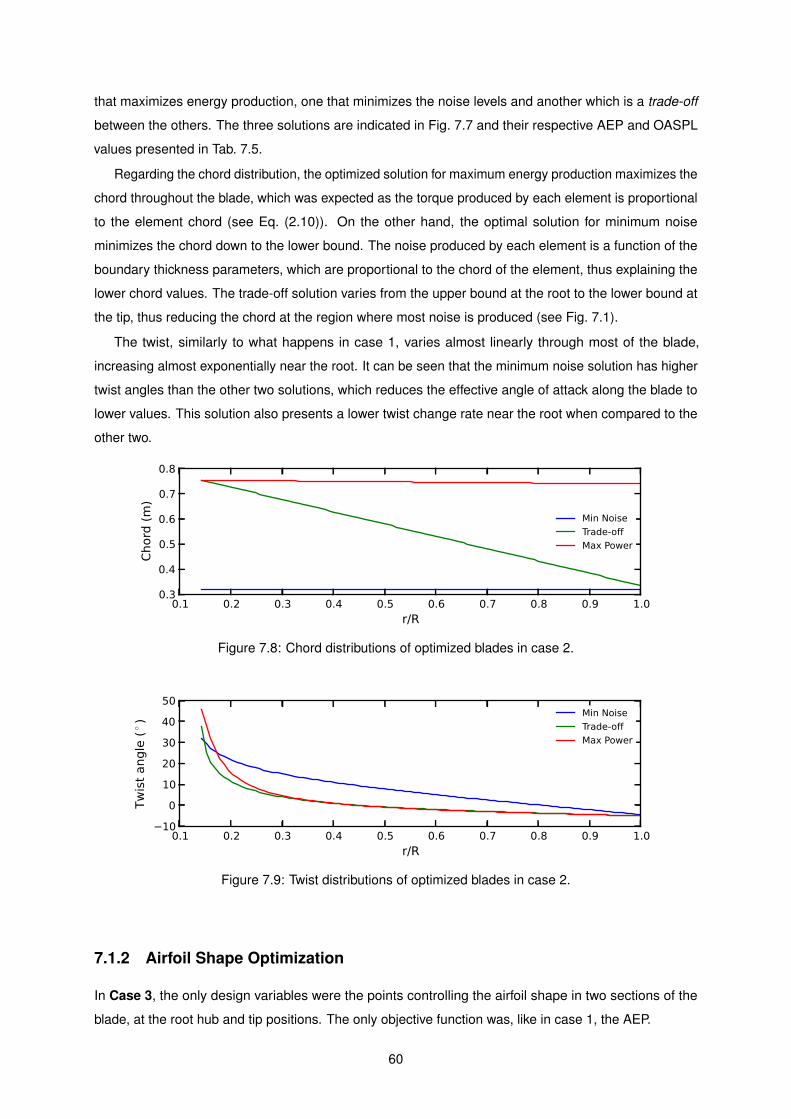
that maximizes energy production, one that minimizes the noise levels and another which is a trade-off

between the others. The three solutions are indicated in Fig. 7.7 and their respective AEP and OASPL

values presented in Tab. 7.5.

Regarding the chord distribution, the optimized solution for maximum energy production maximizes the

chord throughout the blade, which was expected as the torque produced by each element is proportional

to the element chord (see Eq. (2.10)). On the other hand, the optimal solution for minimum noise

minimizes the chord down to the lower bound. The noise produced by each element is a function of the

boundary thickness parameters, which are proportional to the chord of the element, thus explaining the

lower chord values. The trade-off solution varies from the upper bound at the root to the lower bound at

the tip, thus reducing the chord at the region where most noise is produced (see Fig. 7.1).

The twist, similarly to what happens in case 1, varies almost linearly through most of the blade,

increasing almost exponentially near the root. It can be seen that the minimum noise solution has higher

twist angles than the other two solutions, which reduces the effective angle of attack along the blade to

lower values. This solution also presents a lower twist change rate near the root when compared to the

other two.

0.1 0.2 0.3 0.4 0.5 0.6 0.7 0.8 0.9 1.0

r/R

0.3

0.4

0.5

0.6

0.7

0.8

Chord (m)

Min Noise

Trade-off

Max Power

Figure 7.8: Chord distributions of optimized blades in case 2.

0.1 0.2 0.3 0.4 0.5 0.6 0.7 0.8 0.9 1.0

r/R

−10

0

10

20

30

40

50

Tw

ist

angle

(◦ )

Min Noise

Trade-off

Max Power

Figure 7.9: Twist distributions of optimized blades in case 2.

7.1.2 Airfoil Shape Optimization

In Case 3, the only design variables were the points controlling the airfoil shape in two sections of the

blade, at the root hub and tip positions. The only objective function was, like in case 1, the AEP.

60

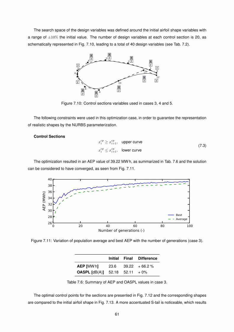
The search space of the design variables was defined around the initial airfoil shape variables with

a range of ±10% the initial value. The number of design variables at each control section is 20, as

schematically represented in Fig. 7.10, leading to a total of 40 design variables (see Tab. 7.2).

yxy

xyx

yx

yx

yx

yxy

x

y

yy

y

Figure 7.10: Control sections variables used in cases 3, 4 and 5.

The following constraints were used in this optimization case, in order to guarantee the representation

of realistic shapes by the NURBS parameterization.

Control Sectionsxcpi ≥ x

cpi+1, upper curve

xcpi ≤ xcpi+1, lower curve

(7.3)

The optimization resulted in an AEP value of 39.22 MW h, as summarized in Tab. 7.6 and the solution

can be considered to have converged, as seen from Fig. 7.11.

0 20 40 60 80 100

Number of generations (-)

26

28

30

32

34

36

38

40

AEP (MWh)

Best

Average

Figure 7.11: Variation of population average and best AEP with the number of generations (case 3).

Initial Final Difference

AEP [MW h] 23.6 39.22 + 66.2 %OASPL [dB(A)] 52.18 52.11 + 0%

Table 7.6: Summary of AEP and OASPL values in case 3.

The optimal control points for the sections are presented in Fig. 7.12 and the corresponding shapes

are compared to the initial airfoil shape in Fig. 7.13. A more accentuated S-tail is noticeable, which results

61

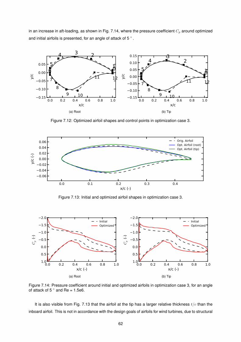
in an increase in aft-loading, as shown in Fig. 7.14, where the pressure coefficient Cp around optimized

and initial airfoils is presented, for an angle of attack of 5 ◦ .

0.0 0.2 0.4 0.6 0.8 1.0

x/c

−0.15

−0.10

−0.05

0.00

0.05

y/c

01

234

56

7

8

9 10

11 12

(a) Root

0.0 0.2 0.4 0.6 0.8 1.0

x/c

−0.15

−0.10

−0.05

0.00

0.05

0.10

0.15

y/c

01

23

4

56

7

89 10

11 12

(b) Tip

Figure 7.12: Optimized airfoil shapes and control points in optimization case 3.

0.0 0.1 0.2 0.3 0.4

x/c (-)

−0.06

−0.04

−0.02

0.00

0.02

0.04

0.06

y/c

(-)

Orig. Airfoil

Opt. Airfoil (root)

Opt. Airfoil (tip)

Figure 7.13: Initial and optimized airfoil shapes in optimization case 3.

0.0 0.2 0.4 0.6 0.8 1.0

x/c (-)

−2.0

−1.5

−1.0

−0.5

0.0

0.5

1.0

Cp (

-)

Initial

Optimized

(a) Root

0.0 0.2 0.4 0.6 0.8 1.0

x/c (-)

−2.0

−1.5

−1.0

−0.5

0.0

0.5

1.0

Cp (

-)

Initial

Optimized

(b) Tip

Figure 7.14: Pressure coefficient around initial and optimized airfoils in optimization case 3, for an angleof attack of 5 ◦ and Re = 1.5e6.

It is also visible from Fig. 7.13 that the airfoil at the tip has a larger relative thickness t/c than the

inboard airfoil. This is not in accordance with the design goals of airfoils for wind turbines, due to structural

62

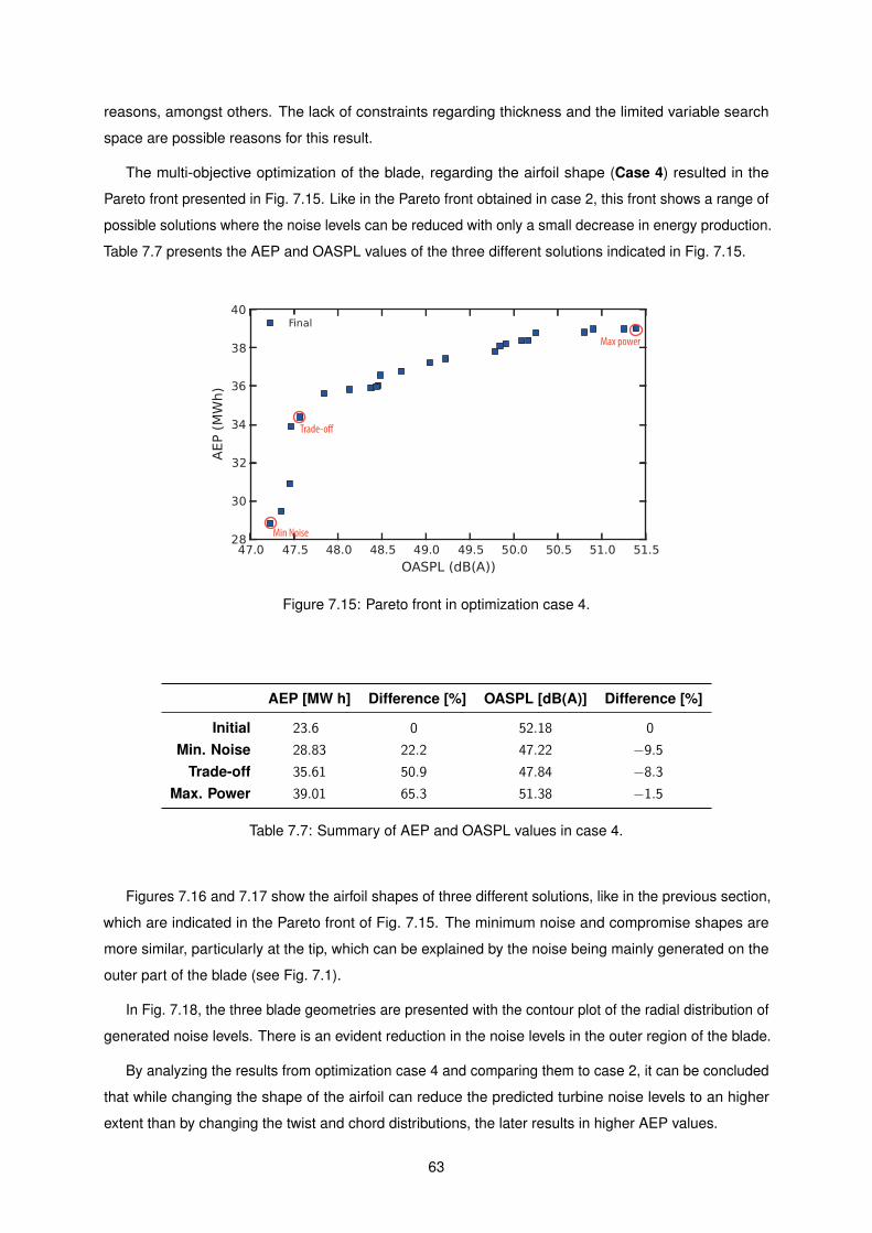
reasons, amongst others. The lack of constraints regarding thickness and the limited variable search

space are possible reasons for this result.

The multi-objective optimization of the blade, regarding the airfoil shape (Case 4) resulted in the

Pareto front presented in Fig. 7.15. Like in the Pareto front obtained in case 2, this front shows a range of

possible solutions where the noise levels can be reduced with only a small decrease in energy production.

Table 7.7 presents the AEP and OASPL values of the three different solutions indicated in Fig. 7.15.

Min Noise

Max power

Trade-o!

Figure 7.15: Pareto front in optimization case 4.

AEP [MW h] Difference [%] OASPL [dB(A)] Difference [%]

Initial 23.6 0 52.18 0

Min. Noise 28.83 22.2 47.22 −9.5Trade-off 35.61 50.9 47.84 −8.3

Max. Power 39.01 65.3 51.38 −1.5

Table 7.7: Summary of AEP and OASPL values in case 4.

Figures 7.16 and 7.17 show the airfoil shapes of three different solutions, like in the previous section,

which are indicated in the Pareto front of Fig. 7.15. The minimum noise and compromise shapes are

more similar, particularly at the tip, which can be explained by the noise being mainly generated on the

outer part of the blade (see Fig. 7.1).

In Fig. 7.18, the three blade geometries are presented with the contour plot of the radial distribution of

generated noise levels. There is an evident reduction in the noise levels in the outer region of the blade.

By analyzing the results from optimization case 4 and comparing them to case 2, it can be concluded

that while changing the shape of the airfoil can reduce the predicted turbine noise levels to an higher

extent than by changing the twist and chord distributions, the later results in higher AEP values.

63

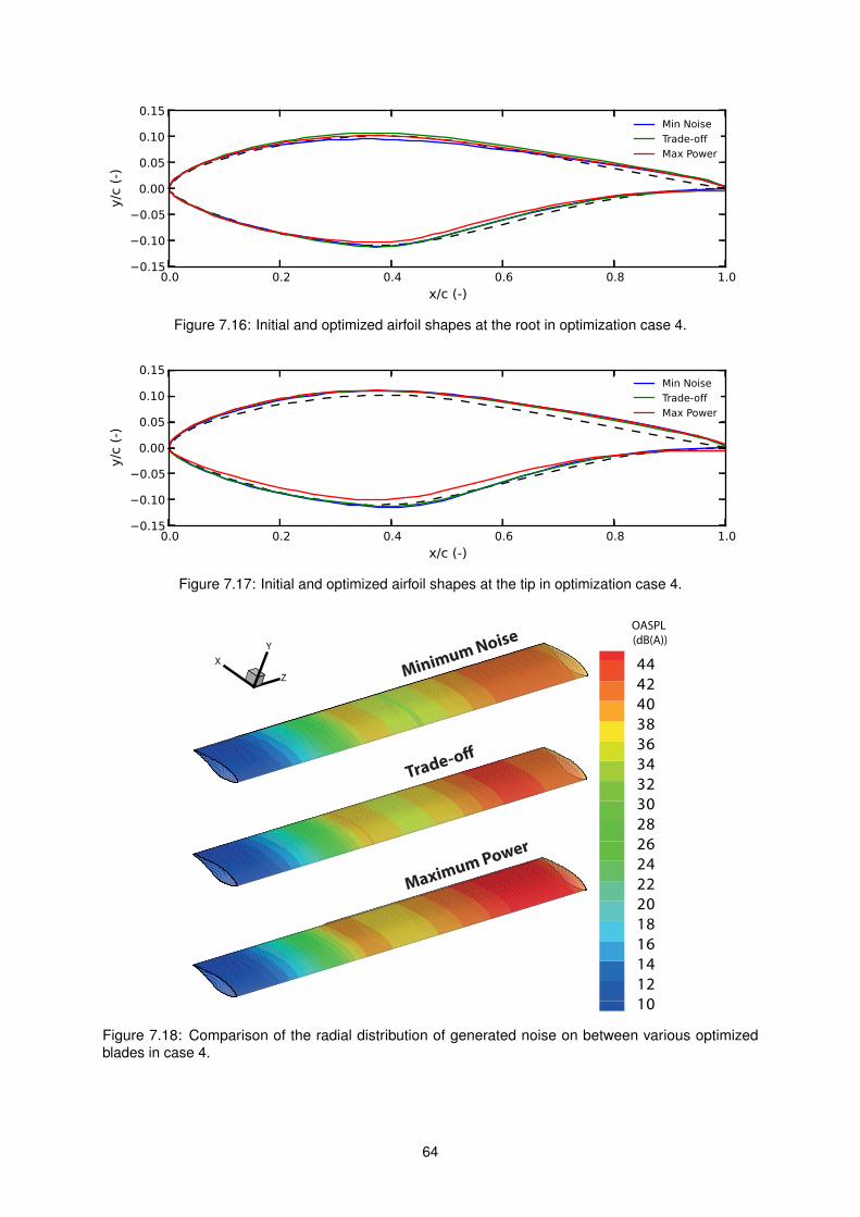
0.0 0.2 0.4 0.6 0.8 1.0

x/c (-)

−0.15

−0.10

−0.05

0.00

0.05

0.10

0.15y/c

(-)

Min Noise

Trade-off

Max Power

Figure 7.16: Initial and optimized airfoil shapes at the root in optimization case 4.

0.0 0.2 0.4 0.6 0.8 1.0

x/c (-)

−0.15

−0.10

−0.05

0.00

0.05

0.10

0.15

y/c

(-)

Min Noise

Trade-off

Max Power

Figure 7.17: Initial and optimized airfoil shapes at the tip in optimization case 4.

44

42

40

38

36

34

32

30

28

26

24

22

20

18

16

14

12

10

OASPL

(dB(A))

Z

X

Y

Minimum Noise

Trade-o�

Maximum Power

Figure 7.18: Comparison of the radial distribution of generated noise on between various optimizedblades in case 4.

64

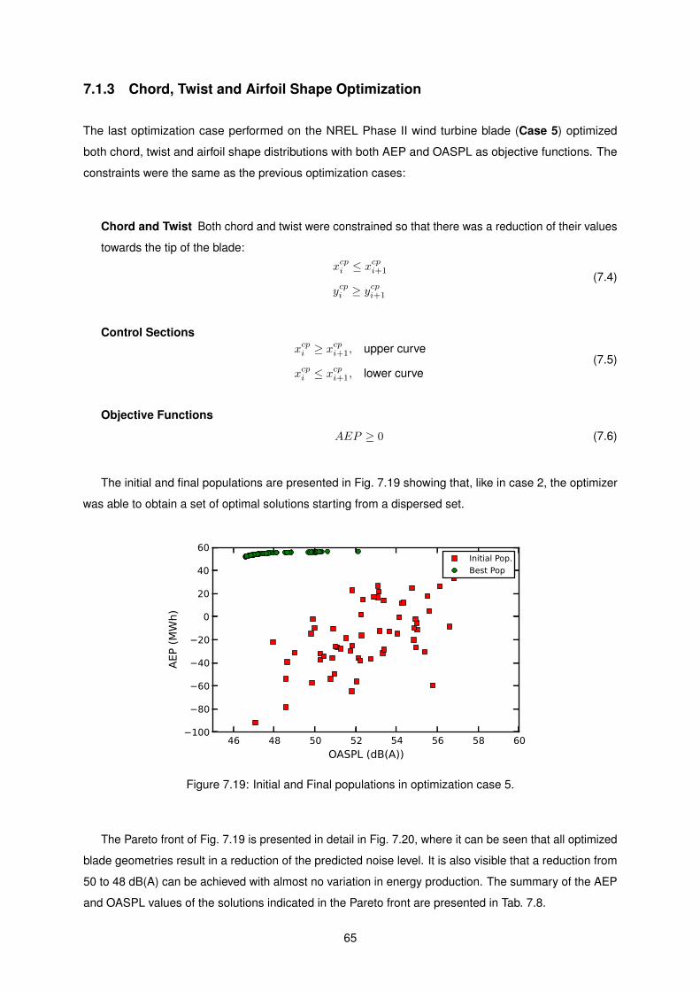
7.1.3 Chord, Twist and Airfoil Shape Optimization

The last optimization case performed on the NREL Phase II wind turbine blade (Case 5) optimized

both chord, twist and airfoil shape distributions with both AEP and OASPL as objective functions. The

constraints were the same as the previous optimization cases:

Chord and Twist Both chord and twist were constrained so that there was a reduction of their values

towards the tip of the blade:

xcpi ≤ xcpi+1

ycpi ≥ ycpi+1

(7.4)

Control Sectionsxcpi ≥ x

cpi+1, upper curve

xcpi ≤ xcpi+1, lower curve

(7.5)

Objective Functions

AEP ≥ 0 (7.6)

The initial and final populations are presented in Fig. 7.19 showing that, like in case 2, the optimizer

was able to obtain a set of optimal solutions starting from a dispersed set.

46 48 50 52 54 56 58 60

OASPL (dB(A))

−100

−80

−60

−40

−20

0

20

40

60

AEP (

MW

h)

Initial Pop.

Best Pop

Figure 7.19: Initial and Final populations in optimization case 5.

The Pareto front of Fig. 7.19 is presented in detail in Fig. 7.20, where it can be seen that all optimized

blade geometries result in a reduction of the predicted noise level. It is also visible that a reduction from

50 to 48 dB(A) can be achieved with almost no variation in energy production. The summary of the AEP

and OASPL values of the solutions indicated in the Pareto front are presented in Tab. 7.8.

65

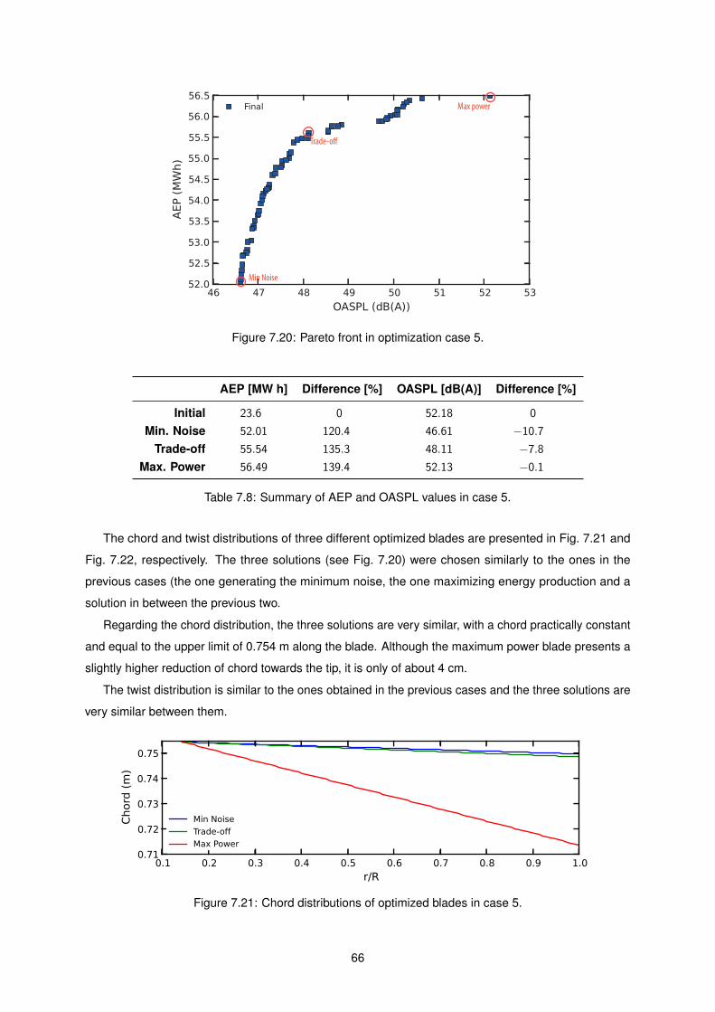
Min Noise

Max power

Trade-o!

Figure 7.20: Pareto front in optimization case 5.

AEP [MW h] Difference [%] OASPL [dB(A)] Difference [%]

Initial 23.6 0 52.18 0

Min. Noise 52.01 120.4 46.61 −10.7Trade-off 55.54 135.3 48.11 −7.8

Max. Power 56.49 139.4 52.13 −0.1

Table 7.8: Summary of AEP and OASPL values in case 5.

The chord and twist distributions of three different optimized blades are presented in Fig. 7.21 and

Fig. 7.22, respectively. The three solutions (see Fig. 7.20) were chosen similarly to the ones in the

previous cases (the one generating the minimum noise, the one maximizing energy production and a

solution in between the previous two.

Regarding the chord distribution, the three solutions are very similar, with a chord practically constant

and equal to the upper limit of 0.754 m along the blade. Although the maximum power blade presents a

slightly higher reduction of chord towards the tip, it is only of about 4 cm.

The twist distribution is similar to the ones obtained in the previous cases and the three solutions are

very similar between them.

0.1 0.2 0.3 0.4 0.5 0.6 0.7 0.8 0.9 1.0

r/R

0.71

0.72

0.73

0.74

0.75

Chord (m)

Min Noise

Trade-off

Max Power

Figure 7.21: Chord distributions of optimized blades in case 5.

66

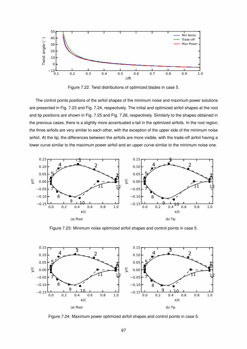
0.1 0.2 0.3 0.4 0.5 0.6 0.7 0.8 0.9 1.0

r/R

−10

0

10

20

30

40

50

Tw

ist

angle

(◦ )

Min Noise

Trade-off

Max Power

Figure 7.22: Twist distributions of optimized blades in case 5.

The control points positions of the airfoil shapes of the minimum noise and maximum power solutions

are presented in Fig. 7.23 and Fig. 7.24, respectively. The initial and optimized airfoil shapes at the root

and tip positions are shown in Fig. 7.25 and Fig. 7.26, respectively. Similarly to the shapes obtained in

the previous cases, there is a slightly more accentuated s-tail in the optimized airfoils. In the root region,

the three airfoils are very similar to each other, with the exception of the upper side of the minimum noise

airfoil. At the tip, the differences between the airfoils are more visible, with the trade-off airfoil having a

lower curve similar to the maximum power airfoil and an upper curve similar to the minimum noise one.

0.0 0.2 0.4 0.6 0.8 1.0

x/c

−0.15

−0.10

−0.05

0.00

0.05

0.10

0.15

y/c

01

23

4

56

7

89 10

11 12

(a) Root

0.0 0.2 0.4 0.6 0.8 1.0

x/c

−0.15

−0.10

−0.05

0.00

0.05

0.10

0.15

y/c

01

23

4

56

7

89 10

11 12

(b) Tip

Figure 7.23: Minimum noise optimized airfoil shapes and control points in case 5.

0.0 0.2 0.4 0.6 0.8 1.0

x/c

−0.15

−0.10

−0.05

0.00

0.05

0.10

0.15

y/c

01

234

56

7

89 10

11 12

(a) Root

0.0 0.2 0.4 0.6 0.8 1.0

x/c

−0.15

−0.10

−0.05

0.00

0.05

0.10

0.15

y/c

01

23

4

56

7

89 10

11 12

(b) Tip

Figure 7.24: Maximum power optimized airfoil shapes and control points in case 5.

67

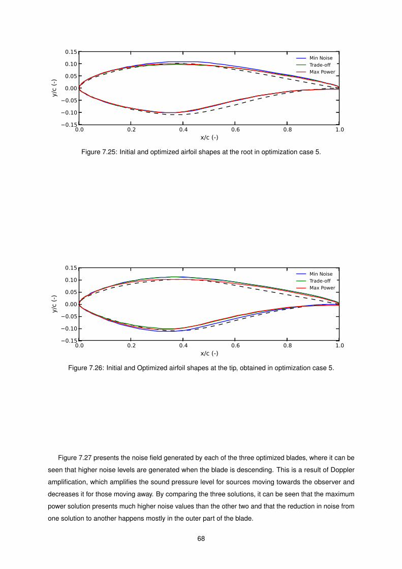
0.0 0.2 0.4 0.6 0.8 1.0

x/c (-)

−0.15

−0.10

−0.05

0.00

0.05

0.10

0.15y/c

(-)

Min Noise

Trade-off

Max Power

Figure 7.25: Initial and optimized airfoil shapes at the root in optimization case 5.

0.0 0.2 0.4 0.6 0.8 1.0

x/c (-)

−0.15

−0.10

−0.05

0.00

0.05

0.10

0.15

y/c

(-)

Min Noise

Trade-off

Max Power

Figure 7.26: Initial and Optimized airfoil shapes at the tip, obtained in optimization case 5.

Figure 7.27 presents the noise field generated by each of the three optimized blades, where it can be

seen that higher noise levels are generated when the blade is descending. This is a result of Doppler

amplification, which amplifies the sound pressure level for sources moving towards the observer and

decreases it for those moving away. By comparing the three solutions, it can be seen that the maximum

power solution presents much higher noise values than the other two and that the reduction in noise from

one solution to another happens mostly in the outer part of the blade.

68

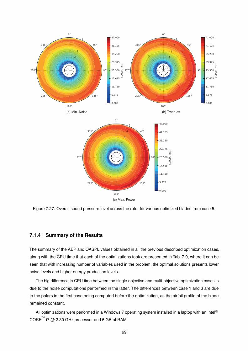
(a) Min. Noise (b) Trade-off

(c) Max. Power

Figure 7.27: Overall sound pressure level across the rotor for various optimized blades from case 5.

7.1.4 Summary of the Results

The summary of the AEP and OASPL values obtained in all the previous described optimization cases,

along with the CPU time that each of the optimizations took are presented in Tab. 7.9, where it can be

seen that with increasing number of variables used in the problem, the optimal solutions presents lower

noise levels and higher energy production levels.

The big difference in CPU time between the single objective and multi-objective optimization cases is

due to the noise computations performed in the latter. The differences between case 1 and 3 are due

to the polars in the first case being computed before the optimization, as the airfoil profile of the blade

remained constant.

All optimizations were performed in a Windows 7 operating system installed in a laptop with an Intel R©

CORETM

i7 @ 2.30 GHz processor and 6 GB of RAM.

69

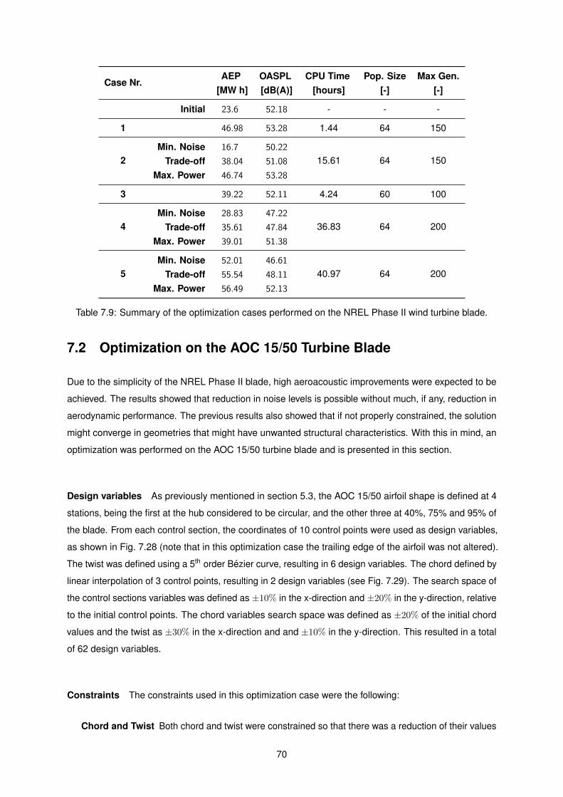
Case Nr.AEP OASPL CPU Time Pop. Size Max Gen.

[MW h] [dB(A)] [hours] [-] [-]

Initial 23.6 52.18 - - -

1 46.98 53.28 1.44 64 150

2Min. Noise 16.7 50.22

15.61 64 150Trade-off 38.04 51.08

Max. Power 46.74 53.28

3 39.22 52.11 4.24 60 100

4Min. Noise 28.83 47.22

36.83 64 200Trade-off 35.61 47.84

Max. Power 39.01 51.38

5Min. Noise 52.01 46.61

40.97 64 200Trade-off 55.54 48.11

Max. Power 56.49 52.13

Table 7.9: Summary of the optimization cases performed on the NREL Phase II wind turbine blade.

7.2 Optimization on the AOC 15/50 Turbine Blade

Due to the simplicity of the NREL Phase II blade, high aeroacoustic improvements were expected to be

achieved. The results showed that reduction in noise levels is possible without much, if any, reduction in

aerodynamic performance. The previous results also showed that if not properly constrained, the solution

might converge in geometries that might have unwanted structural characteristics. With this in mind, an

optimization was performed on the AOC 15/50 turbine blade and is presented in this section.

Design variables As previously mentioned in section 5.3, the AOC 15/50 airfoil shape is defined at 4

stations, being the first at the hub considered to be circular, and the other three at 40%, 75% and 95% of

the blade. From each control section, the coordinates of 10 control points were used as design variables,

as shown in Fig. 7.28 (note that in this optimization case the trailing edge of the airfoil was not altered).

The twist was defined using a 5th order Bezier curve, resulting in 6 design variables. The chord defined by

linear interpolation of 3 control points, resulting in 2 design variables (see Fig. 7.29). The search space of

the control sections variables was defined as ±10% in the x-direction and ±20% in the y-direction, relative

to the initial control points. The chord variables search space was defined as ±20% of the initial chord

values and the twist as ±30% in the x-direction and and ±10% in the y-direction. This resulted in a total

of 62 design variables.

Constraints The constraints used in this optimization case were the following:

Chord and Twist Both chord and twist were constrained so that there was a reduction of their values

70

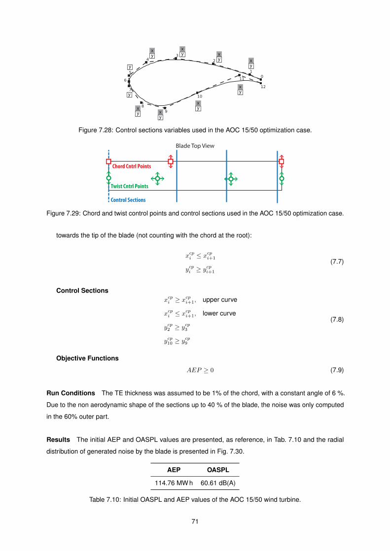
yxy

xyx

yx

yx

yx

yxy

x

y

y

Figure 7.28: Control sections variables used in the AOC 15/50 optimization case.

Control Sections

Chord Cntrl Points

Twist Cntrl Points

Blade Top View

Figure 7.29: Chord and twist control points and control sections used in the AOC 15/50 optimization case.

towards the tip of the blade (not counting with the chord at the root):

xcpi ≤ xcpi+1

ycpi ≥ ycpi+1

(7.7)

Control Sectionsxcpi ≥ x

cpi+1, upper curve

xcpi ≤ xcpi+1, lower curve

ycp2 ≥ ycp3

ycp10 ≥ ycp9

(7.8)

Objective Functions

AEP ≥ 0 (7.9)

Run Conditions The TE thickness was assumed to be 1% of the chord, with a constant angle of 6 %.

Due to the non aerodynamic shape of the sections up to 40 % of the blade, the noise was only computed

in the 60% outer part.

Results The initial AEP and OASPL values are presented, as reference, in Tab. 7.10 and the radial

distribution of generated noise by the blade is presented in Fig. 7.30.

AEP OASPL

114.76 MW h 60.61 dB(A)

Table 7.10: Initial OASPL and AEP values of the AOC 15/50 wind turbine.

71

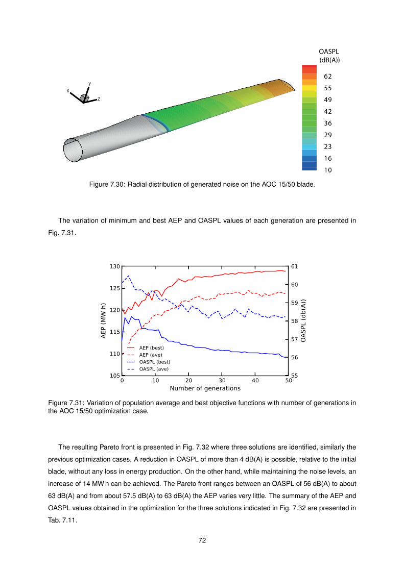
X

Y

Z

OASPL

(dB(A))

62

55

49

42

36

29

23

16

10

Figure 7.30: Radial distribution of generated noise on the AOC 15/50 blade.

The variation of minimum and best AEP and OASPL values of each generation are presented in

Fig. 7.31.

0 10 20 30 40 50

Number of generations

105

110

115

120

125

130

AEP (MW h)

55

56

57

58

59

60

61

OASPL (db(A))

AEP (best)

AEP (ave)

OASPL (best)

OASPL (ave)

Figure 7.31: Variation of population average and best objective functions with number of generations inthe AOC 15/50 optimization case.

The resulting Pareto front is presented in Fig. 7.32 where three solutions are identified, similarly the

previous optimization cases. A reduction in OASPL of more than 4 dB(A) is possible, relative to the initial

blade, without any loss in energy production. On the other hand, while maintaining the noise levels, an

increase of 14 MW h can be achieved. The Pareto front ranges between an OASPL of 56 dB(A) to about

63 dB(A) and from about 57.5 dB(A) to 63 dB(A) the AEP varies very little. The summary of the AEP and

OASPL values obtained in the optimization for the three solutions indicated in Fig. 7.32 are presented in

Tab. 7.11.

72

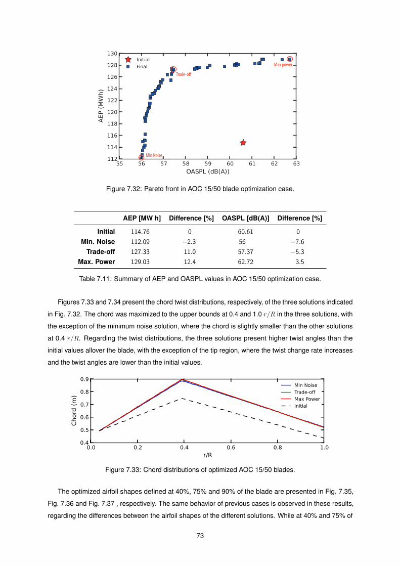
Min Noise

Max power

Trade-o!

Figure 7.32: Pareto front in AOC 15/50 blade optimization case.

AEP [MW h] Difference [%] OASPL [dB(A)] Difference [%]

Initial 114.76 0 60.61 0

Min. Noise 112.09 −2.3 56 −7.6Trade-off 127.33 11.0 57.37 −5.3

Max. Power 129.03 12.4 62.72 3.5

Table 7.11: Summary of AEP and OASPL values in AOC 15/50 optimization case.

Figures 7.33 and 7.34 present the chord twist distributions, respectively, of the three solutions indicated

in Fig. 7.32. The chord was maximized to the upper bounds at 0.4 and 1.0 r/R in the three solutions, with

the exception of the minimum noise solution, where the chord is slightly smaller than the other solutions

at 0.4 r/R. Regarding the twist distributions, the three solutions present higher twist angles than the

initial values allover the blade, with the exception of the tip region, where the twist change rate increases

and the twist angles are lower than the initial values.

0.0 0.2 0.4 0.6 0.8 1.0

r/R

0.4

0.5

0.6

0.7

0.8

0.9

Chord

(m

)

Min Noise

Trade-off

Max Power

Initial

Figure 7.33: Chord distributions of optimized AOC 15/50 blades.

The optimized airfoil shapes defined at 40%, 75% and 90% of the blade are presented in Fig. 7.35,

Fig. 7.36 and Fig. 7.37 , respectively. The same behavior of previous cases is observed in these results,

regarding the differences between the airfoil shapes of the different solutions. While at 40% and 75% of

73

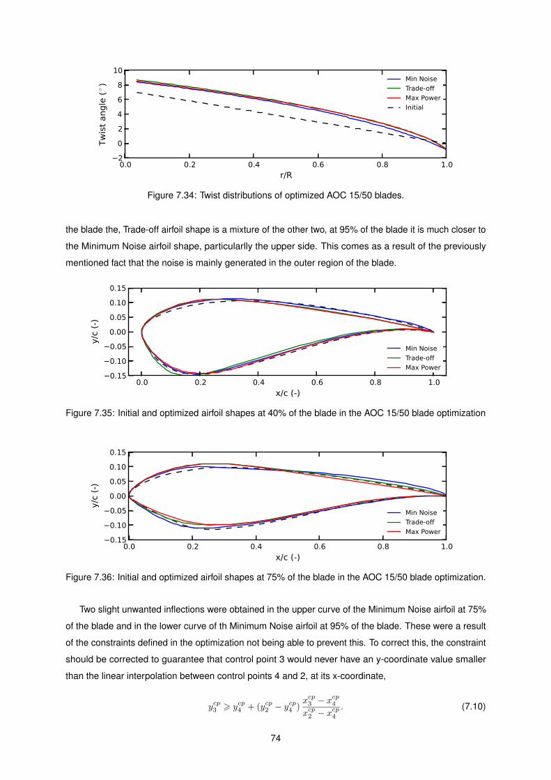
0.0 0.2 0.4 0.6 0.8 1.0

r/R

−2

0

2

4

6

8

10

Tw

ist

angle

(◦ )

Min Noise

Trade-off

Max Power

Initial

Figure 7.34: Twist distributions of optimized AOC 15/50 blades.

the blade the, Trade-off airfoil shape is a mixture of the other two, at 95% of the blade it is much closer to

the Minimum Noise airfoil shape, particularlly the upper side. This comes as a result of the previously

mentioned fact that the noise is mainly generated in the outer region of the blade.

0.0 0.2 0.4 0.6 0.8 1.0

x/c (-)

−0.15

−0.10

−0.05

0.00

0.05

0.10

0.15

y/c

(-)

Min Noise

Trade-off

Max Power

Figure 7.35: Initial and optimized airfoil shapes at 40% of the blade in the AOC 15/50 blade optimization

0.0 0.2 0.4 0.6 0.8 1.0

x/c (-)

−0.15

−0.10

−0.05

0.00

0.05

0.10

0.15

y/c

(-)

Min Noise

Trade-off

Max Power

Figure 7.36: Initial and optimized airfoil shapes at 75% of the blade in the AOC 15/50 blade optimization.

Two slight unwanted inflections were obtained in the upper curve of the Minimum Noise airfoil at 75%

of the blade and in the lower curve of th Minimum Noise airfoil at 95% of the blade. These were a result

of the constraints defined in the optimization not being able to prevent this. To correct this, the constraint

should be corrected to guarantee that control point 3 would never have an y-coordinate value smaller

than the linear interpolation between control points 4 and 2, at its x-coordinate,

ycp3 > ycp4 + (ycp2 − ycp4 )

xcp3 − xcp4

xcp2 − xcp4

. (7.10)

74

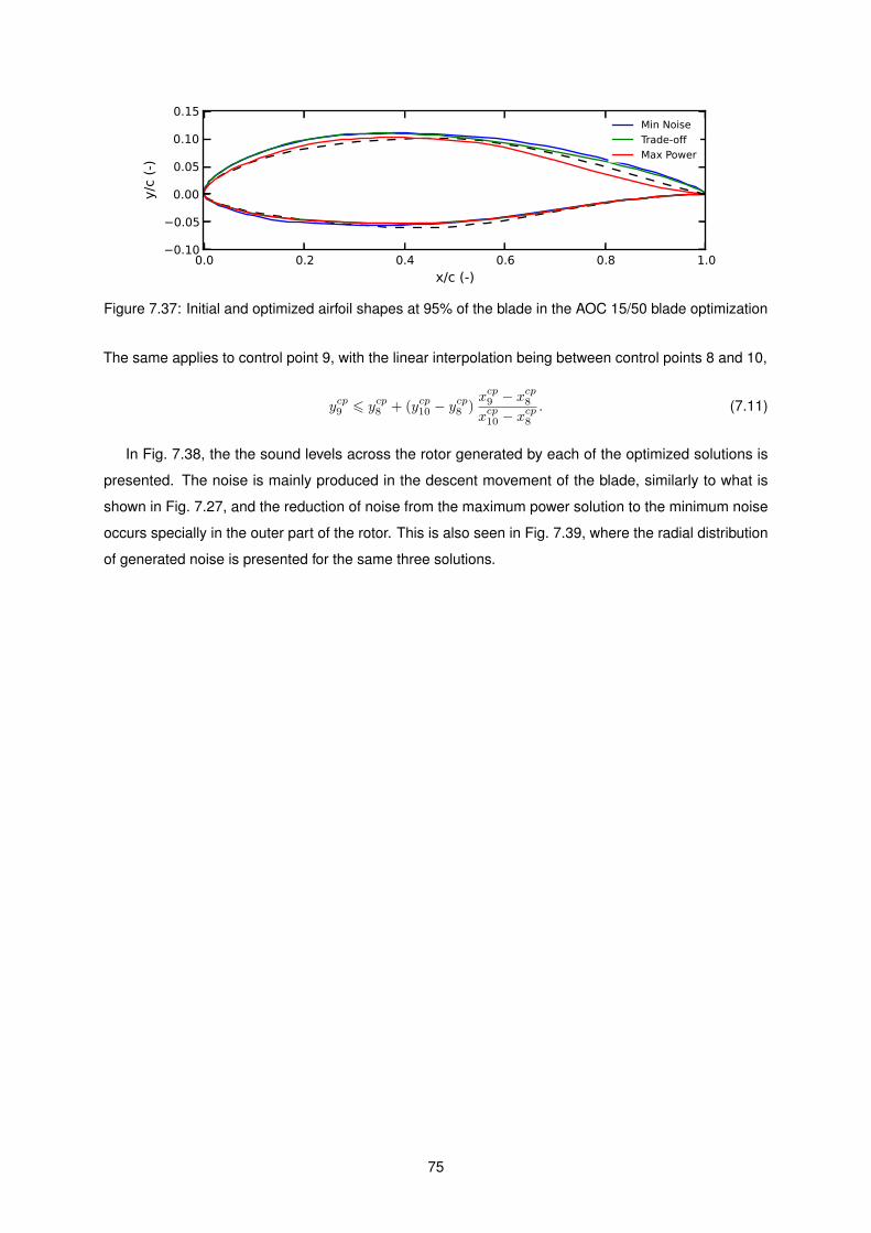
0.0 0.2 0.4 0.6 0.8 1.0

x/c (-)

−0.10

−0.05

0.00

0.05

0.10

0.15

y/c

(-)

Min Noise

Trade-off

Max Power

Figure 7.37: Initial and optimized airfoil shapes at 95% of the blade in the AOC 15/50 blade optimization

The same applies to control point 9, with the linear interpolation being between control points 8 and 10,

ycp9 6 ycp8 + (ycp10 − ycp8 )

xcp9 − xcp8

xcp10 − xcp8

. (7.11)

In Fig. 7.38, the the sound levels across the rotor generated by each of the optimized solutions is

presented. The noise is mainly produced in the descent movement of the blade, similarly to what is

shown in Fig. 7.27, and the reduction of noise from the maximum power solution to the minimum noise

occurs specially in the outer part of the rotor. This is also seen in Fig. 7.39, where the radial distribution

of generated noise is presented for the same three solutions.

75

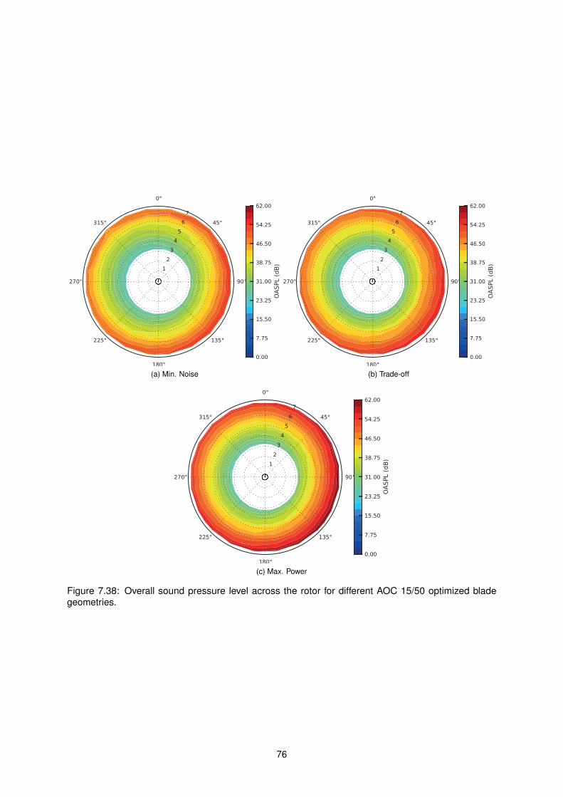
(a) Min. Noise (b) Trade-off

(c) Max. Power

Figure 7.38: Overall sound pressure level across the rotor for different AOC 15/50 optimized bladegeometries.

76

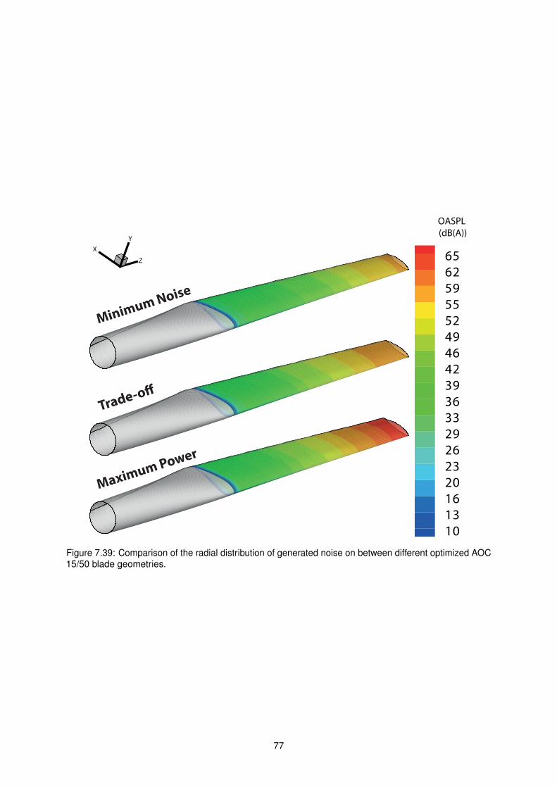
65

62

59

55

52

49

46

42

39

36

33

29

26

23

20

16

13

10

OASPL

(dB(A))

Z

X

Y

Minimum Noise

Trade-o�

Maximum Power

Figure 7.39: Comparison of the radial distribution of generated noise on between different optimized AOC15/50 blade geometries.

77

78

Chapter 8

Conclusions

In this chapter, a summary of what was achieved during this work is presented, followed by some

suggestions for the improvement of the aeroacoustic prediction and design framework.

8.1 Achievements

In the present work, a wind turbine aerodynamic and aeroacoustic prediction model was successfully

implemented and validated against experimental data. The code developed is flexible, with various

inputs and options, allowing the control of the simulations in detail. It is able to output the results of the

simulations in various formats for post-processing.

A geometrical model of the wind turbine blade was also developed and implemented, using NURBS

curves and Bezier curves, for the definition of the cross sectional airfoil shapes and twist and chord

distributions, respectively. The NURBS parameterization of the airfoil shapes proved to be a good

approach, as it was able to accurately reproduce various different airfoil shapes commonly used in wind

turbines.

The code was successfully implemented into an optimization framework, being able to produce optimal

solutions in the various performed optimizations. In the optimizations performed on the NREL Phase

II wind turbine, a maximum increase in AEP of 139.4 % and maximum reduction of OASPL in 10.7 %

was achieved. This large relative improvements showed that this particular blade was far from being

optimal. In contrast, using another blade, from the commercially available AOC 15/50 wind turbine, it

was possible to assess more realistically the potential of the optimization framework. In this case, the

optimization resulted in a maximum improvement in AEP of 12.4 % and a maximum OASPL reduction of

7.6 %. However, these results were not achieved in the same blade geometry, and the trade-off between

noise generation and energy production is visible in the results of the optimizations.

Nowadays, with wind turbine blade geometries being so optimized, tools like the framework developed

are used in the design phase of any wind turbine to increase the wind turbines performance to the

maximum possible extent, as it might make a big difference in terms of the commercial success of the

wind turbine. The relative small computational requirement of each optimization is a key factor, as it

79

allows for a greater diversity of geometries and configurations to be analyzed / optimized, thus increasing

the probability of obtaining a better solution.

8.2 Future Work

There were two issues that occurred during the optimizations that would be interesting to address. The

first one is related to the constraints. It would be interesting to perform optimization of the blade with a

new set of constraints and a larger search space, allowing for different airfoil shapes to be tested. The

second was the numerical precision of the solutions saved by pyOpt’s NSGA-II optimizer. The analysis of

the final solutions given by the optimizer were not in total agreement with the values obtained during the

optimization, thus indicating that more precision is needed in the data saved to files.

Regarding the wind turbine aerodynamic model itself, some improvements could be introduced.

Moving to an unsteady BEM model or to a vortex wake method would improve the accuracy of the results

and, coupled to a structural model, allow for the optimization of both aerodynamics, acoustics, and

structural behavior or the wind turbine rotor.

Another improvement that would be interesting to see implemented in the code is the use of parallel

processing to reduce the amount of CPU-time required by each optimization and thus allowing a higher

refinement of the models or even the use of more complex models. This is rather simple to implement

in a GA algorithm, as in each generation, the evaluation of the objective functions for each individual is

done independently.

One last suggestion is to perform single objective optimizations with constraints on the generated

noise, instead of multi-objective optimizations. The results of the optimizations provided Pareto fronts

with solutions that, while producing a large increase in energy production, also increased the noise levels.

As the maximum noise levels allowed are usually legislated (see chapter 1), a maximum noise level could

be set as a constraint, thus forcing the optimizer to focus its search in a region where legal noise levels

would be produced.

80

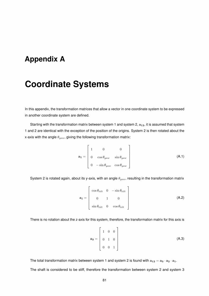
Appendix A

Coordinate Systems

In this appendix, the transformation matrices that allow a vector in one coordinate system to be expressed

in another coordinate system are defined.

Starting with the transformation matrix between system 1 and system 2, a12, it is assumed that system

1 and 2 are identical with the exception of the position of the origins. System 2 is then rotated about the

x-axis with the angle θyaw, giving the following transformation matrix:

a1 =

1 0 0

0 cos θyaw sin θyaw

0 − sin θyaw cos θyaw

(A.1)

System 2 is rotated again, about its y-axis, with an angle θyaw, resulting in the transformation matrix

a2 =

cos θtilt 0 − sin θtilt

0 1 0

sin θtilt 0 cos θtilt

(A.2)

There is no rotation about the z-axis for this system, therefore, the transformation matrix for this axis is

a3 =

1 0 0

0 1 0

0 0 1

(A.3)

The total transformation matrix between system 1 and system 2 is found with a12 = a3 · a2 · a1.

The shaft is considered to be stiff, therefore the transformation between system 2 and system 3

81

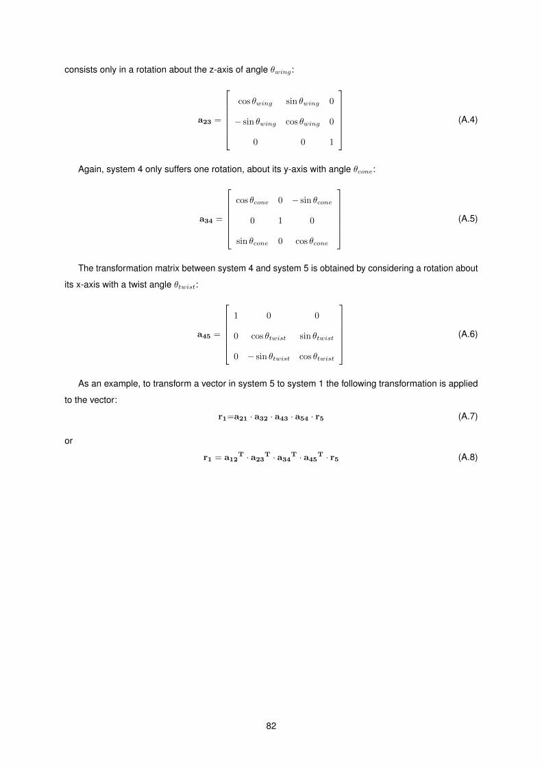
consists only in a rotation about the z-axis of angle θwing:

a23 =

cos θwing sin θwing 0

− sin θwing cos θwing 0

0 0 1

(A.4)

Again, system 4 only suffers one rotation, about its y-axis with angle θcone:

a34 =

cos θcone 0 − sin θcone

0 1 0

sin θcone 0 cos θcone

(A.5)

The transformation matrix between system 4 and system 5 is obtained by considering a rotation about

its x-axis with a twist angle θtwist:

a45 =

1 0 0

0 cos θtwist sin θtwist

0 − sin θtwist cos θtwist

(A.6)

As an example, to transform a vector in system 5 to system 1 the following transformation is applied

to the vector:

r1=a21 · a32 · a43 · a54 · r5 (A.7)

or

r1 = a12T · a23T · a34T · a45T · r5 (A.8)

82

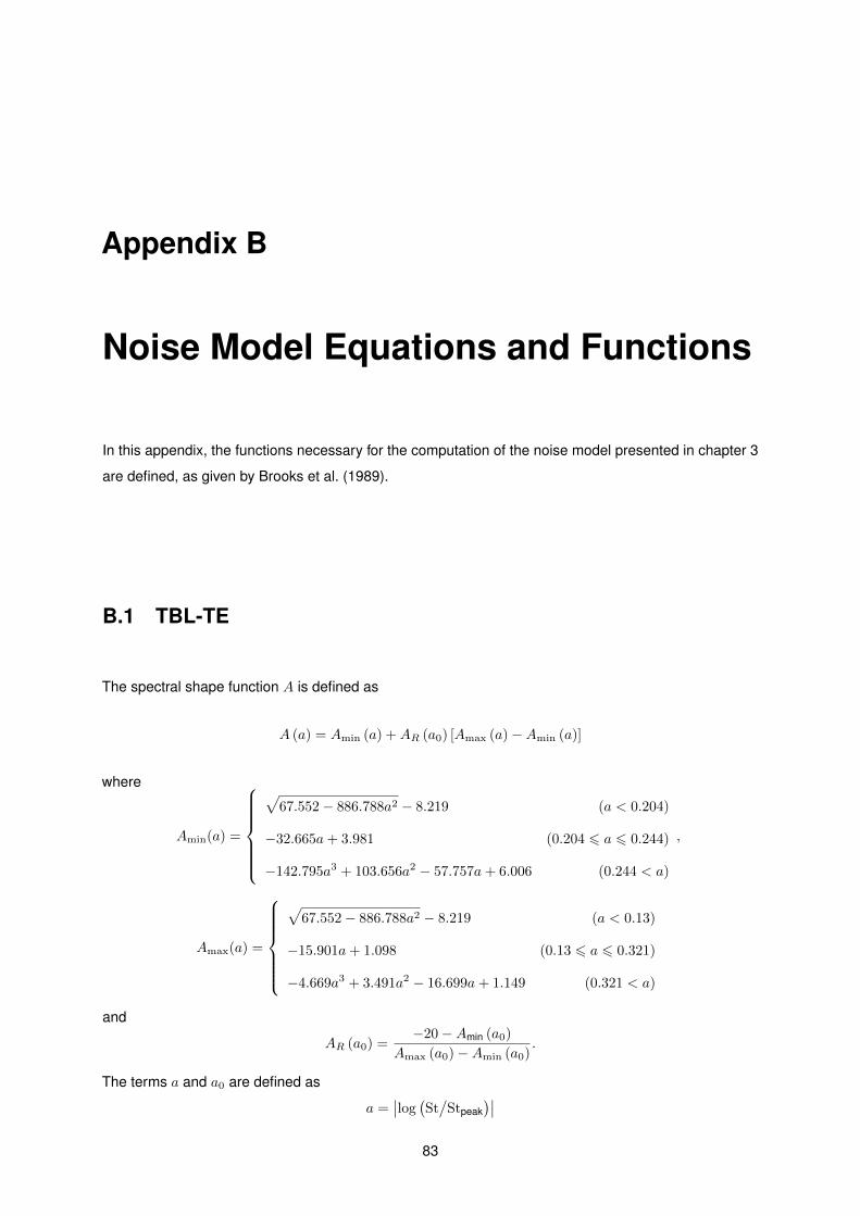
Appendix B

Noise Model Equations and Functions

In this appendix, the functions necessary for the computation of the noise model presented in chapter 3

are defined, as given by Brooks et al. (1989).

B.1 TBL-TE

The spectral shape function A is defined as

A (a) = Amin (a) +AR (a0) [Amax (a)−Amin (a)]

where

Amin(a) =

√67.552− 886.788a2 − 8.219

−32.665a+ 3.981

−142.795a3 + 103.656a2 − 57.757a+ 6.006

(a < 0.204)

(0.204 6 a 6 0.244)

(0.244 < a)

,

Amax(a) =

√67.552− 886.788a2 − 8.219

−15.901a+ 1.098

−4.669a3 + 3.491a2 − 16.699a+ 1.149

(a < 0.13)

(0.13 6 a 6 0.321)

(0.321 < a)

and

AR (a0) =−20−Amin (a0)

Amax (a0)−Amin (a0).

The terms a and a0 are defined as

a =∣∣log

(St/

Stpeak)∣∣

83

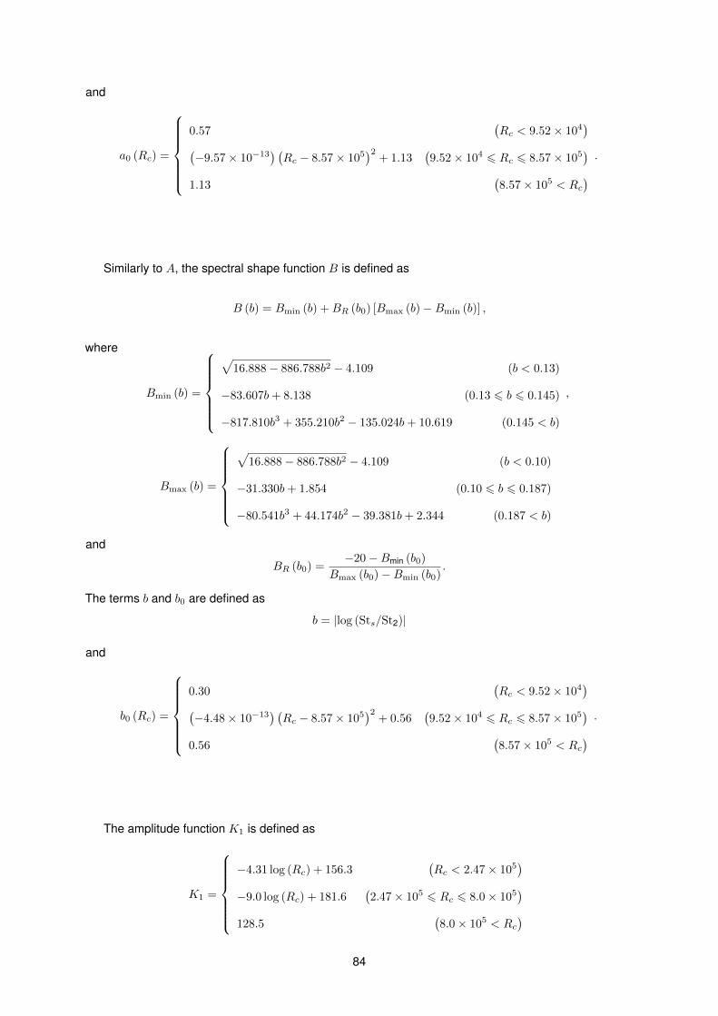
and

a0 (Rc) =

0.57(−9.57× 10−13

) (Rc − 8.57× 105

)2+ 1.13

1.13

(Rc < 9.52× 104

)(9.52× 104 6 Rc 6 8.57× 105

)(8.57× 105 < Rc

) .

Similarly to A, the spectral shape function B is defined as

B (b) = Bmin (b) +BR (b0) [Bmax (b)−Bmin (b)] ,

where

Bmin (b) =

√16.888− 886.788b2 − 4.109

−83.607b+ 8.138

−817.810b3 + 355.210b2 − 135.024b+ 10.619

(b < 0.13)

(0.13 6 b 6 0.145)

(0.145 < b)

,

Bmax (b) =

√16.888− 886.788b2 − 4.109

−31.330b+ 1.854

−80.541b3 + 44.174b2 − 39.381b+ 2.344

(b < 0.10)

(0.10 6 b 6 0.187)

(0.187 < b)

and

BR (b0) =−20−Bmin (b0)

Bmax (b0)−Bmin (b0).

The terms b and b0 are defined as

b = |log (Sts/St2)|

and

b0 (Rc) =

0.30(−4.48× 10−13

) (Rc − 8.57× 105

)2+ 0.56

0.56

(Rc < 9.52× 104

)(9.52× 104 6 Rc 6 8.57× 105

)(8.57× 105 < Rc

) .

The amplitude function K1 is defined as

K1 =

−4.31 log (Rc) + 156.3

−9.0 log (Rc) + 181.6

128.5

(Rc < 2.47× 105

)(2.47× 105 6 Rc 6 8.0× 105

)(8.0× 105 < Rc

)84

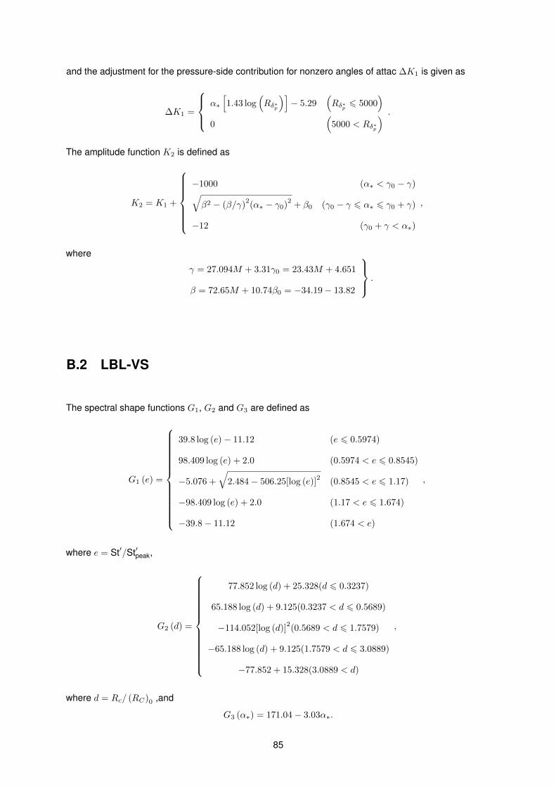
and the adjustment for the pressure-side contribution for nonzero angles of attac ∆K1 is given as

∆K1 =

α∗

[1.43 log

(Rδ∗p

)]− 5.29

0

(Rδ∗p 6 5000

)(

5000 < Rδ∗p

) .

The amplitude function K2 is defined as

K2 = K1 +

−1000√β2 − (β/γ)

2(α∗ − γ0)

2+ β0

−12

(α∗ < γ0 − γ)

(γ0 − γ 6 α∗ 6 γ0 + γ)

(γ0 + γ < α∗)

,

where

γ = 27.094M + 3.31γ0 = 23.43M + 4.651

β = 72.65M + 10.74β0 = −34.19− 13.82

.

B.2 LBL-VS

The spectral shape functions G1, G2 and G3 are defined as

G1 (e) =

39.8 log (e)− 11.12 (e 6 0.5974)

98.409 log (e) + 2.0 (0.5974 < e 6 0.8545)

−5.076 +

√2.484− 506.25[log (e)]

2(0.8545 < e 6 1.17)

−98.409 log (e) + 2.0 (1.17 < e 6 1.674)

−39.8− 11.12 (1.674 < e)

,

where e = St′/St′peak,

G2 (d) =

77.852 log (d) + 25.328(d 6 0.3237)

65.188 log (d) + 9.125(0.3237 < d 6 0.5689)

−114.052[log (d)]2(0.5689 < d 6 1.7579)

−65.188 log (d) + 9.125(1.7579 < d 6 3.0889)

−77.852 + 15.328(3.0889 < d)

,

where d = Rc/ (RC)0 ,and

G3 (α∗) = 171.04− 3.03α∗.

85

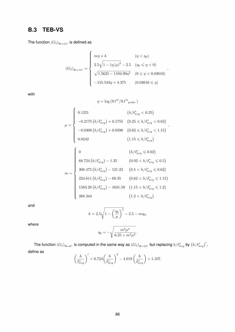
B.3 TEB-VS

The function (G5)Ψ=14◦ is defined as

(G5)Ψ=14◦ =

mη + k (η < η0)

2.5

√1− (η/µ)

2 − 2.5 (η0 6 η < 0)√1.5625− 1194.99η2 (0 6 η < 0.03616)

−155.543η + 4.375 (0.03616 6 η)

,

with

η = log (S t′′′/S t′′′peak, )

µ =

0.1221(h/δ∗avg < 0.25

)−0.2175

(h/δ∗avg

)+ 0.1755

(0.25 6 h/δ∗avg < 0.62

)−0.0308

(h/δ∗avg

)+ 0.0596

(0.62 6 h/δ∗avg < 1.15

)0.0242

(1.15 6 h/δ∗avg

),

m =

0(h/δ∗avg 6 0.02

)68.724

(h/δ∗avg

)− 1.35

(0.02 < h/δ∗avg 6 0.5

)308.475

(h/δ∗avg

)− 121.23

(0.5 < h/δ∗avg 6 0.62

)224.811

(h/δ∗avg

)− 69.35

(0.62 < h/δ∗avg 6 1.15

)1583.28

(h/δ∗avg

)− 1631.59

(1.15 < h/δ∗avg 6 1.2

)268.344

(1.2 < h/δ∗avg

)and

k = 2.5

√1−

(η0

µ

)2

− 2.5−mη0,

where

η0 = −

√m2µ4

6.25 +m2µ2.

The function (G5)Ψ=0◦ is computed in the same way as (G5)Ψ=14◦ but replacing h/δ∗avg by(h/δ∗avg

)′,define as (

h

δ∗avg

)′= 6.724

(h

δ∗avg

)2

− 4.019

(h

δ∗avg

)+ 1.107.

86

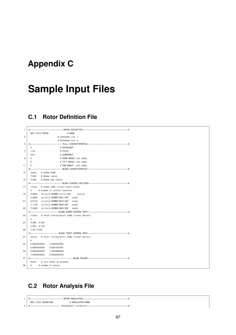
Appendix C

Sample Input Files

C.1 Rotor Definition File

1 #−−−−−−−−−−−−−−−−−−−−−−−−−−− ROTOR DEFINITION−−−−−−−−−−−−−−−−−−−−−−−−−−−−−−−−−−−−−#

AOC 15/50 ROTOR # NAME

3 # Comments l i n e 1

# Comments l i n e 2

5 #−−−−−−−−−−−−−−−−−−−−−−−−−− Rotor CHARACTERISTICS−−−−−−−−−−−−−−−−−−−−−−−−−−−−−−−−−#

3 # NR BLADES

7 1.54 # PITCH

24.4 # HUBHEIGHT

9 0 # CONE ANGLE ( not used )

0 # TILT ANGLE ( not used )

11 0 # YAW ANGLE ( not used )

#−−−−−−−−−−−−−−−−−−−−−−−−−− BLADE CHARACTERISTICS−−−−−−−−−−−−−−−−−−−−−−−−−−−−−−−−−#

13 nurbs # blade mode

7.490 # Blade rad ius

15 0.280 # Blade hub rad ius

#−−−−−−−−−−−−−−−−−−−−−−−−−− BLADE CONTROL SECTIOSN−−−−−−−−−−−−−−−−−−−−−−−−−−−−−−−−#

17 l i n e a r # blade mode ( f i x e d / l i n e a r / nurbs )

5 # number o f c o n t r o l sec t ions

19 0.2800 a i r f o i l s /NURBS/ c i r c l e .DAT n c i r c l e

2.9960 a i r f o i l s /NURBS/ S821 .DAT nurbs

21 5.6175 a i r f o i l s /NURBS/ S819 .DAT nurbs

7.1155 a i r f o i l s /NURBS/ S820 .DAT nurbs

23 7.4900 a i r f o i l s /NURBS/ S820 .DAT nurbs

#−−−−−−−−−−−−−−−−−−−−−−− BLADE CHORD CONTROL PNTS−−−−−−−−−−−−−−−−−−−−−−−−−−−−−−−−−#

25 l i n e a r # chord i n t e r p o l a t i o n mode ( l i n e a r / bez ie r )

3

27 0.280 0.494

2.925 0.749

29 7.49 0.436

#−−−−−−−−−−−−−−−−−−−−−−− BLADE TWIST CONTROL PNTS−−−−−−−−−−−−−−−−−−−−−−−−−−−−−−−−−#

31 bez ie r # t w i s t i n t e r p o l a t i o n mode ( l i n e a r / bez ie r )

4

33 0.2800000000 7.0000000000

2.9960000000 4.3631067961

35 5.9920000000 1.4543689320

7.4900000000 0.0000000000

37 #−−−−−−−−−−−−−−−−−−−−−−−−−−−−−−−−−−− BLADE POLARS−−−−−−−−−−−−−−−−−−−−−−−−−−−−−−−−−#

blank # l e f t b lank on purpose

39 0 # number o f po la rs

C.2 Rotor Analysis File

1 #−−−−−−−−−−−−−−−−−−−−−−−−−−− ROTOR SIMULATION−−−−−−−−−−−−−−−−−−−−−−−−−−−−−−−−−−−−−#

AOC 15/50 ANANLYSIS # SIMULATION NAME

3 #−−−−−−−−−−−−−−−−−−−−−−−−− Atmospheric cond i t i ons−−−−−−−−−−−−−−−−−−−−−−−−−−−−−−−−−#

87

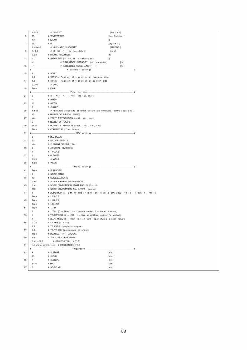
1.225 # DENSITY [ kg / m3]

5 20 # TEMPERATURE [ deg Celc ius ]

1.4 # GAMMA [ ]

7 287 # R [ Jkg−1K−1]

1.46e−5 # KINEMATIC VISCOSITY [M2/SEC ]

9 340.4 # C0 ( i f −1 i t i s ca l cu la ted ) [m/ s ]

0.08 # GROUND ROUGHNESS [m]

11 −1 # SHEAR EXP ( i f −1, i t i s ca l cu la ted ) [ ]

−1 # TURBULENCE INTENSITY (−1: computed ) [%]

13 −1 # TURBULENCE SCALE LENGHT ” ” [m]

#−−−−−−−−−−−−−−−−−−−−−−−−−−− X f o i l / R f o i l s e t t i n g s−−−−−−−−−−−−−−−−−−−−−−−−−−−−−−−−−#

15 9 # NCRIT

1.0 # XTR P− Pos i t i on o f t r a n s i t i o n a t pressure s ide

17 1.0 # XTR S− Pos i t i on o f t r a n s i t i o n a t suc t ion s ide

0.005 # VACC

19 True # PANE

#−−−−−−−−−−−−−−−−−−−−−−−−−−−−−− Polar s e t t i n g s−−−−−−−−−−−−−−−−−−−−−−−−−−−−−−−−−−−−#

21 0 # 0− X f o i l / 1− R f o i l ( f o r BL only )

−1 # A NEG

23 10 # A POS

1 # A STEP

25 1.5e6 # REYNOLDS ( reynolds a t which po la rs are computed , comma separated )

151 # NUMPER OF AIRFOIL POINTS

27 s in # POINT DISTRIBUTION ( un i f , s in , cos )

5 # NUMBER OF POLARS

29 sect # POLAR DISTRIBUTION ( sect , un i f , s in , cos )

True # CORRECT 3D ( True / False )

31 #−−−−−−−−−−−−−−−−−−−−−−−−−−−−−−−−−−− BEM s e t t i n g s−−−−−−−−−−−−−−−−−−−−−−−−−−−−−−−−−#

0 # BEM DEBUG

33 50 # NR OF ELEMENTS

s in # ELEMENT DISTRIBUTION

35 4 # AZIMUTAL DIVISIONS

1 # TIPLOSS

37 1 # HUBLOSS

6.48 # WEI A

39 1.99 # WEI K

#−−−−−−−−−−−−−−−−−−−−−−−−−−−−−−−−− Noise s e t t i n g s−−−−−−−−−−−−−−−−−−−−−−−−−−−−−−−−−#

41 True # RUN NOISE

0 # NOISE DEBUG

43 10 # NOISE ELEMENTS

u n i f # NOISE ELEMENT DISTRIBUTION

45 0.4 # NOISE COMPUTATION START RADIUS (0−1.0)

100 # NOISE COMPUTATION AoA CUTOFF ( degree )

47 3 # BL METHOD (0= BPM, no t r i p ; 1=BPM l i g h t t r i p ; 2= BPM eavy t r i p ; 3 = x f o i l ; 4 = r f o i l )

True # I TBLTE

49 True # I LBLVS

True # I BLUNT

51 True # I T IP

2 # I T IN (0 − None ; 1− Lowsons model ; 2− Amiet ’ s model )

53 1 # TIN METHOD (0 − Off ; 1− Use s i m p l i f i e d gu ida t i ’ s method )

1 # BLUNT MODE (0 − from f o i l ; 1−from inpu t (%) ; 2−d i r e c t value )

55 0.75 # C2 PER (1−x ac )

6.0 # TE ANGLE ( angle i n degree )

57 1.0 # TE PTHICK ( percentage of chord )

True # ROUNDED TIP − LOGICAL

59 1.0 # TIP LIFT CURVE SLOPE

0 0 −32.5 # OBS POSITION (X Y Z)

61 runs / m a r c o l i n i . f r eq # FREQUENCIES FILE

#−−−−−−−−−−−−−−−−−−−−−−−−−−−−−−−−− Operat ion−−−−−−−−−−−−−−−−−−−−−−−−−−−−−−−−−−−−−−#

63 4 # U START [m/ s ]

25 # U END [m/ s ]

65 1 # U STEPS [m/ s ]

64.6 # RPM [ rpm ]

67 6 # NOISE VEL [m/ s ]

88

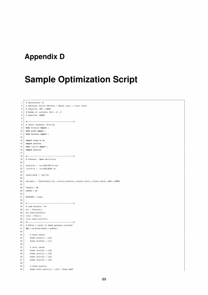
Appendix D

Sample Optimization Script

1 # Opt im iza t ion 10

2 # Optimizes Cont ro l Sect ions + Bezier t w i s t + l i n e a r chord

3 # Objec t i ve : AEP + OASPL

4 # Number o f v a r i a b l e s 18∗3 + 6 + 2

5 # Algor i thm : NSGA2

6

7 #−−−−−−−−−−−−−−−−−−−−−−−−−−−−−−−−−−−−−−−−−−−−#

8 # Impor t necessary l i b r a r i e s

9 from Analys is import ∗

10 from pyOpt import ∗

11 from Geometry import ∗

12

13 import numpy as np

14 import datet ime

15 from z i p f i l e import ∗

16 import datet ime

17

18 #−−−−−−−−−−−−−−−−−−−−−−−−−−−−−−−−−−−−−−−−−−−−#

19 # Filename / Name d e f i n i t i o n s

20

21 a n a l yF i l e = ’ run / AOC OPT 10 . an l ’

22 r o t o r F i l e = ’ run /AOC NLB3 . r o t ’

23

24 output name = ’ opt 10c ’

25

26 opt name = ’ Opt im iza t ion 10− c o n t r o l sec t ions + bez ie r t w i s t + l i n e a r chord − AEP + OASPL ’

27

28 PopSize = 68

29 maxGen = 50

30

31 HOTSTART = False

32

33 #−−−−−−−−−−−−−−−−−−−−−−−−−−−−−−−−−−−−−−−−−−−−#

34 # Load Ana lys is f i l e

35 anl = Ana lys is ( )

36 an l . load ( a n a l yF i l e )

37 r o t o r = Rotor ( )

38 r o t o r . load ( r o t o r F i l e )

39 #−−−−−−−−−−−−−−−−−−−−−−−−−−−−−−−−−−−−−−−−−−−−#

40 # Def ine x vec to r to blade geometry conver te r

41 def x to b lade ( blade , x , g=None ) :

42

43 # chord values

44 blade . chord [ 1 ] = x [ 0 ]

45 blade . chord [ 2 ] = x [ 1 ]

46

47 # t w i s t values

48 blade . t w i s t [ 0 ] = x [ 2 ]

49 blade . t w i s t [ 1 ] = x [ 3 ]

50 blade . t w i s t [ 2 ] = x [ 4 ]

51 blade . t w i s t [ 3 ] = x [ 5 ]

52

53 # chord p o s i t i o n

54 blade . t w i s t r a d i u s [ 1 ] = x [ 6 ] ∗ blade .maxR

89

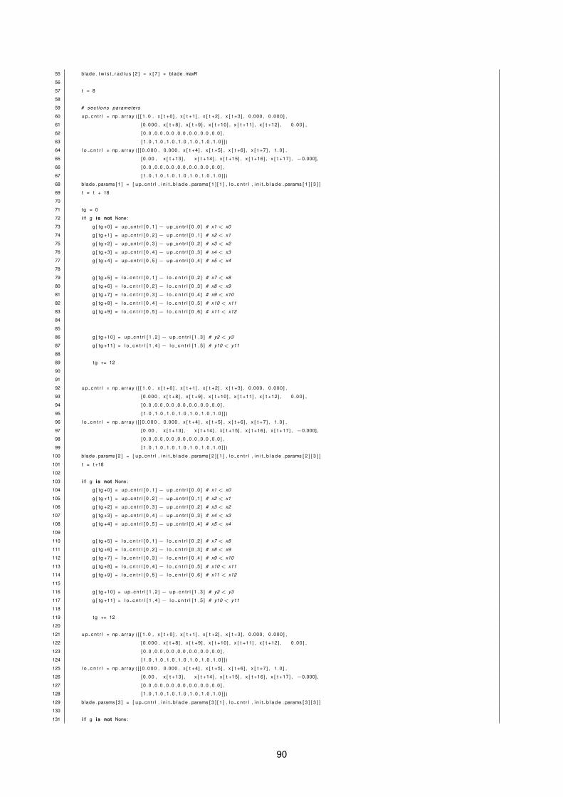
55 blade . t w i s t r a d i u s [ 2 ] = x [ 7 ] ∗ blade .maxR

56

57 t = 8

58

59 # sec t ions parameters

60 u p c n t r l = np . ar ray ( [ [ 1 . 0 , x [ t +0 ] , x [ t +1] , x [ t +2] , x [ t +3] , 0.000 , 0 .000 ] ,

61 [0 .000 , x [ t +8] , x [ t +9] , x [ t +10] , x [ t +11] , x [ t +12] , 0 .00 ] ,

62 [ 0 . 0 , 0 . 0 , 0 . 0 , 0 . 0 , 0 . 0 , 0 . 0 , 0 . 0 ] ,

63 [ 1 . 0 , 1 . 0 , 1 . 0 , 1 . 0 , 1 . 0 , 1 . 0 , 1 . 0 ] ] )

64 l o c n t r l = np . ar ray ( [ [ 0 . 0 0 0 , 0.000 , x [ t +4] , x [ t +5] , x [ t +6] , x [ t +7 ] , 1 . 0 ] ,

65 [0 .00 , x [ t +13] , x [ t +14] , x [ t +15] , x [ t +16] , x [ t +17] , −0.000] ,

66 [ 0 . 0 , 0 . 0 , 0 . 0 , 0 . 0 , 0 . 0 , 0 . 0 , 0 . 0 ] ,

67 [ 1 . 0 , 1 . 0 , 1 . 0 , 1 . 0 , 1 . 0 , 1 . 0 , 1 . 0 ] ] )

68 blade . params [ 1 ] = [ u p c n t r l , i n i t b l a d e . params [ 1 ] [ 1 ] , l o c n t r l , i n i t b l a d e . params [ 1 ] [ 3 ] ]

69 t = t + 18

70

71 tg = 0

72 i f g is not None :

73 g [ tg +0] = u p c n t r l [ 0 , 1 ] − u p c n t r l [ 0 , 0 ] # x1 < x0

74 g [ tg +1] = u p c n t r l [ 0 , 2 ] − u p c n t r l [ 0 , 1 ] # x2 < x1

75 g [ tg +2] = u p c n t r l [ 0 , 3 ] − u p c n t r l [ 0 , 2 ] # x3 < x2

76 g [ tg +3] = u p c n t r l [ 0 , 4 ] − u p c n t r l [ 0 , 3 ] # x4 < x3

77 g [ tg +4] = u p c n t r l [ 0 , 5 ] − u p c n t r l [ 0 , 4 ] # x5 < x4

78

79 g [ tg +5] = l o c n t r l [ 0 , 1 ] − l o c n t r l [ 0 , 2 ] # x7 < x8

80 g [ tg +6] = l o c n t r l [ 0 , 2 ] − l o c n t r l [ 0 , 3 ] # x8 < x9

81 g [ tg +7] = l o c n t r l [ 0 , 3 ] − l o c n t r l [ 0 , 4 ] # x9 < x10

82 g [ tg +8] = l o c n t r l [ 0 , 4 ] − l o c n t r l [ 0 , 5 ] # x10 < x11

83 g [ tg +9] = l o c n t r l [ 0 , 5 ] − l o c n t r l [ 0 , 6 ] # x11 < x12

84

85

86 g [ tg +10] = u p c n t r l [ 1 , 2 ] − u p c n t r l [ 1 , 3 ] # y2 < y3

87 g [ tg +11] = l o c n t r l [ 1 , 4 ] − l o c n t r l [ 1 , 5 ] # y10 < y11

88

89 tg += 12

90

91

92 u p c n t r l = np . ar ray ( [ [ 1 . 0 , x [ t +0 ] , x [ t +1] , x [ t +2] , x [ t +3] , 0.000 , 0 .000 ] ,

93 [0 .000 , x [ t +8] , x [ t +9] , x [ t +10] , x [ t +11] , x [ t +12] , 0 .00 ] ,

94 [ 0 . 0 , 0 . 0 , 0 . 0 , 0 . 0 , 0 . 0 , 0 . 0 , 0 . 0 ] ,

95 [ 1 . 0 , 1 . 0 , 1 . 0 , 1 . 0 , 1 . 0 , 1 . 0 , 1 . 0 ] ] )

96 l o c n t r l = np . ar ray ( [ [ 0 . 0 0 0 , 0.000 , x [ t +4] , x [ t +5] , x [ t +6] , x [ t +7 ] , 1 . 0 ] ,

97 [0 .00 , x [ t +13] , x [ t +14] , x [ t +15] , x [ t +16] , x [ t +17] , −0.000] ,

98 [ 0 . 0 , 0 . 0 , 0 . 0 , 0 . 0 , 0 . 0 , 0 . 0 , 0 . 0 ] ,

99 [ 1 . 0 , 1 . 0 , 1 . 0 , 1 . 0 , 1 . 0 , 1 . 0 , 1 . 0 ] ] )

100 blade . params [ 2 ] = [ u p c n t r l , i n i t b l a d e . params [ 2 ] [ 1 ] , l o c n t r l , i n i t b l a d e . params [ 2 ] [ 3 ] ]

101 t = t +18

102

103 i f g is not None :

104 g [ tg +0] = u p c n t r l [ 0 , 1 ] − u p c n t r l [ 0 , 0 ] # x1 < x0

105 g [ tg +1] = u p c n t r l [ 0 , 2 ] − u p c n t r l [ 0 , 1 ] # x2 < x1

106 g [ tg +2] = u p c n t r l [ 0 , 3 ] − u p c n t r l [ 0 , 2 ] # x3 < x2

107 g [ tg +3] = u p c n t r l [ 0 , 4 ] − u p c n t r l [ 0 , 3 ] # x4 < x3

108 g [ tg +4] = u p c n t r l [ 0 , 5 ] − u p c n t r l [ 0 , 4 ] # x5 < x4

109

110 g [ tg +5] = l o c n t r l [ 0 , 1 ] − l o c n t r l [ 0 , 2 ] # x7 < x8

111 g [ tg +6] = l o c n t r l [ 0 , 2 ] − l o c n t r l [ 0 , 3 ] # x8 < x9

112 g [ tg +7] = l o c n t r l [ 0 , 3 ] − l o c n t r l [ 0 , 4 ] # x9 < x10

113 g [ tg +8] = l o c n t r l [ 0 , 4 ] − l o c n t r l [ 0 , 5 ] # x10 < x11

114 g [ tg +9] = l o c n t r l [ 0 , 5 ] − l o c n t r l [ 0 , 6 ] # x11 < x12

115

116 g [ tg +10] = u p c n t r l [ 1 , 2 ] − u p c n t r l [ 1 , 3 ] # y2 < y3

117 g [ tg +11] = l o c n t r l [ 1 , 4 ] − l o c n t r l [ 1 , 5 ] # y10 < y11

118

119 tg += 12

120

121 u p c n t r l = np . ar ray ( [ [ 1 . 0 , x [ t +0 ] , x [ t +1] , x [ t +2] , x [ t +3] , 0.000 , 0 .000 ] ,

122 [0 .000 , x [ t +8] , x [ t +9] , x [ t +10] , x [ t +11] , x [ t +12] , 0 .00 ] ,

123 [ 0 . 0 , 0 . 0 , 0 . 0 , 0 . 0 , 0 . 0 , 0 . 0 , 0 . 0 ] ,

124 [ 1 . 0 , 1 . 0 , 1 . 0 , 1 . 0 , 1 . 0 , 1 . 0 , 1 . 0 ] ] )

125 l o c n t r l = np . ar ray ( [ [ 0 . 0 0 0 , 0.000 , x [ t +4] , x [ t +5] , x [ t +6] , x [ t +7 ] , 1 . 0 ] ,

126 [0 .00 , x [ t +13] , x [ t +14] , x [ t +15] , x [ t +16] , x [ t +17] , −0.000] ,

127 [ 0 . 0 , 0 . 0 , 0 . 0 , 0 . 0 , 0 . 0 , 0 . 0 , 0 . 0 ] ,

128 [ 1 . 0 , 1 . 0 , 1 . 0 , 1 . 0 , 1 . 0 , 1 . 0 , 1 . 0 ] ] )

129 blade . params [ 3 ] = [ u p c n t r l , i n i t b l a d e . params [ 3 ] [ 1 ] , l o c n t r l , i n i t b l a d e . params [ 3 ] [ 3 ] ]

130

131 i f g is not None :

90

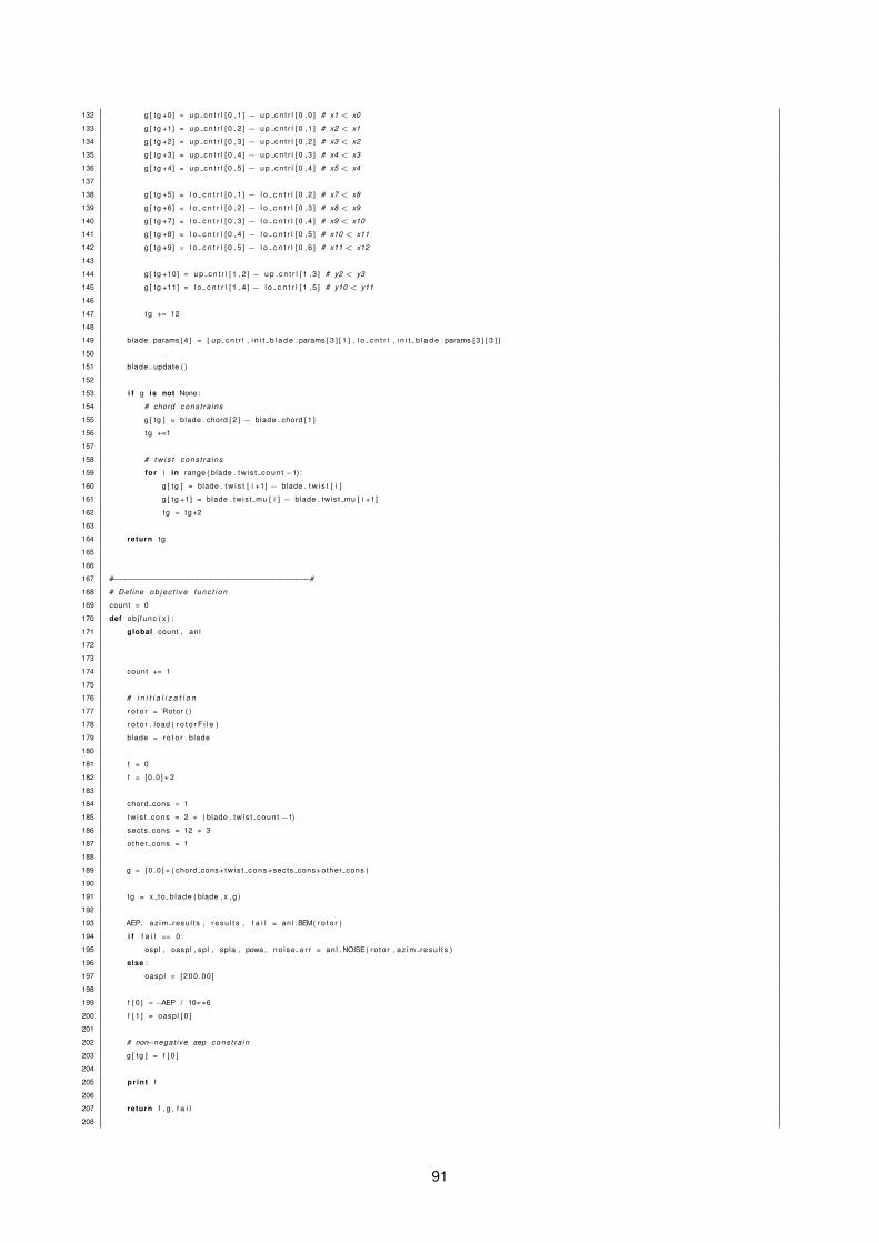
132 g [ tg +0] = u p c n t r l [ 0 , 1 ] − u p c n t r l [ 0 , 0 ] # x1 < x0

133 g [ tg +1] = u p c n t r l [ 0 , 2 ] − u p c n t r l [ 0 , 1 ] # x2 < x1

134 g [ tg +2] = u p c n t r l [ 0 , 3 ] − u p c n t r l [ 0 , 2 ] # x3 < x2

135 g [ tg +3] = u p c n t r l [ 0 , 4 ] − u p c n t r l [ 0 , 3 ] # x4 < x3

136 g [ tg +4] = u p c n t r l [ 0 , 5 ] − u p c n t r l [ 0 , 4 ] # x5 < x4

137

138 g [ tg +5] = l o c n t r l [ 0 , 1 ] − l o c n t r l [ 0 , 2 ] # x7 < x8

139 g [ tg +6] = l o c n t r l [ 0 , 2 ] − l o c n t r l [ 0 , 3 ] # x8 < x9

140 g [ tg +7] = l o c n t r l [ 0 , 3 ] − l o c n t r l [ 0 , 4 ] # x9 < x10

141 g [ tg +8] = l o c n t r l [ 0 , 4 ] − l o c n t r l [ 0 , 5 ] # x10 < x11

142 g [ tg +9] = l o c n t r l [ 0 , 5 ] − l o c n t r l [ 0 , 6 ] # x11 < x12

143

144 g [ tg +10] = u p c n t r l [ 1 , 2 ] − u p c n t r l [ 1 , 3 ] # y2 < y3

145 g [ tg +11] = l o c n t r l [ 1 , 4 ] − l o c n t r l [ 1 , 5 ] # y10 < y11

146

147 tg += 12

148

149 blade . params [ 4 ] = [ u p c n t r l , i n i t b l a d e . params [ 3 ] [ 1 ] , l o c n t r l , i n i t b l a d e . params [ 3 ] [ 3 ] ]

150

151 blade . update ( )

152

153 i f g is not None :

154 # chord cons t ra ins

155 g [ tg ] = blade . chord [ 2 ] − blade . chord [ 1 ]

156 tg +=1

157

158 # t w i s t cons t ra ins

159 for i in range ( blade . tw i s t coun t−1) :

160 g [ tg ] = blade . t w i s t [ i +1] − blade . t w i s t [ i ]

161 g [ tg +1] = blade . tw is t mu [ i ] − blade . tw is t mu [ i +1]

162 tg = tg +2

163

164 return tg

165

166

167 #−−−−−−−−−−−−−−−−−−−−−−−−−−−−−−−−−−−−−−−−−−−−#

168 # Def ine o b j e c t i v e f u n c t i o n

169 count = 0

170 def ob j func ( x ) :

171 global count , an l

172

173

174 count += 1

175

176 # i n i t i a l i z a t i o n

177 r o t o r = Rotor ( )

178 r o t o r . load ( r o t o r F i l e )

179 blade = r o t o r . blade

180

181 t = 0

182 f = [0 .0 ]∗2

183

184 chord cons = 1

185 tw i s t cons = 2 ∗ ( blade . tw i s t coun t−1)

186 sects cons = 12 ∗ 3

187 other cons = 1

188

189 g = [ 0 . 0 ]∗ ( chord cons+ tw i s t cons +sects cons+other cons )

190

191 tg = x to b lade ( blade , x , g )

192

193 AEP, az im resu l t s , r e su l t s , f a i l = an l .BEM( r o t o r )

194 i f f a i l == 0 :

195 ospl , oaspl , spl , spla , powa , n o i s e e r r = an l . NOISE( ro to r , az im resu l t s )

196 else :

197 oaspl = [200 .00 ]

198

199 f [ 0 ] =−AEP / 10∗∗6

200 f [ 1 ] = oaspl [ 0 ]

201

202 # non−negat ive aep cons t ra i n

203 g [ tg ] = f [ 0 ]

204

205 pr in t f

206

207 return f , g , f a i l

208

91

209 #−−−−−−−−−−−−−−−−−−−−−−−−−−−−−−−−−−−−−−−−−−−−#

210 # Def ine pyOpt o p t i m i z a t i o n problem

211 opt prob = Opt im iza t ion ( opt name , ob j func )

212

213 i n i t r o t o r = Rotor ( )

214 i n i t r o t o r . load ( r o t o r F i l e )

215 i n i t b l a d e = i n i t r o t o r . blade

216

217 #−−−−−−−−−−−−− Add Objec t i ve−−−−−−−−−−−−−−−−#

218 opt prob . addObj ( ’AEP ’ )

219 opt prob . addObj ( ’OASPL ’ )

220 #−−−−−−−−−−−−− Add Var iab les−−−−−−−−−−−−−−−−#

221

222 lower chord = np . ar ray ( i n i t b l a d e . chord ) − 0.2 ∗ abs ( np . ar ray ( i n i t b l a d e . chord ) )

223 upper chord = np . ar ray ( i n i t b l a d e . chord ) + 0.2 ∗ abs ( np . ar ray ( i n i t b l a d e . chord ) )

224

225 opt prob . addVar ( ’ cyy2 ’ , ’ c ’ , lower = lower chord [ 1 ] , upper = upper chord [ 1 ] , value = i n i t b l a d e . chord [ 1 ] )

226 opt prob . addVar ( ’ cyy3 ’ , ’ c ’ , lower = lower chord [ 2 ] , upper = upper chord [ 2 ] , value = i n i t b l a d e . chord [ 2 ] )

227

228 l o w e r t w i s t = np . ar ray ( i n i t b l a d e . t w i s t ) − 0.1 ∗ abs ( np . ar ray ( i n i t b l a d e . t w i s t ) )

229 u p p e r t w i s t = np . ar ray ( i n i t b l a d e . t w i s t ) + 0.1 ∗ abs ( np . ar ray ( i n i t b l a d e . t w i s t ) )

230

231 opt prob . addVar ( ’ tyy1 ’ , ’ c ’ , lower = l o w e r t w i s t [ 0 ] , upper = u p p e r t w i s t [ 0 ] , value = i n i t b l a d e . t w i s t [ 0 ] )

232 opt prob . addVar ( ’ tyy2 ’ , ’ c ’ , lower = l o w e r t w i s t [ 1 ] , upper = u p p e r t w i s t [ 1 ] , value = i n i t b l a d e . t w i s t [ 1 ] )

233 opt prob . addVar ( ’ tyy3 ’ , ’ c ’ , lower = l o w e r t w i s t [ 2 ] , upper = u p p e r t w i s t [ 2 ] , value = i n i t b l a d e . t w i s t [ 2 ] )

234 opt prob . addVar ( ’ tyy4 ’ , ’ c ’ , lower = l o w e r t w i s t [ 3 ] , upper = u p p e r t w i s t [ 3 ] , value = i n i t b l a d e . t w i s t [ 3 ] )

235

236 l o w e r t w i s t = np . ar ray ( i n i t b l a d e . tw is t mu ) − 0.3 ∗ abs ( np . ar ray ( i n i t b l a d e . tw is t mu ) )

237 u p p e r t w i s t = np . ar ray ( i n i t b l a d e . tw is t mu ) + 0.3 ∗ abs ( np . ar ray ( i n i t b l a d e . tw is t mu ) )

238

239 opt prob . addVar ( ’ txx2 ’ , ’ c ’ , lower = l o w e r t w i s t [ 1 ] , upper = u p p e r t w i s t [ 1 ] , value = i n i t b l a d e . tw is t mu [ 1 ] )

240 opt prob . addVar ( ’ txx3 ’ , ’ c ’ , lower = l o w e r t w i s t [ 2 ] , upper = u p p e r t w i s t [ 2 ] , value = i n i t b l a d e . tw is t mu [ 2 ] )

241

242 for j in range ( i n i t b l a d e . sects count−2) :

243

244 k = j +1

245

246 v a r i x = 0.1

247 v a r i y = 0.2

248

249 # Upper curve x

250 lower up x = np . maximum( i n i t b l a d e . params [ k ] [ 0 ] [ 0 , : ] − abs ( i n i t b l a d e . params [ k ] [ 0 ] [ 0 , : ] ) ∗ v a r i x , 0 . 0 )

251 upper up x = np . minimum ( i n i t b l a d e . params [ k ] [ 0 ] [ 0 , : ] + abs ( i n i t b l a d e . params [ k ] [ 0 ] [ 0 , : ] ) ∗ v a r i x , 1 . 0 )

252 # Lower curve x

253 l o w e r l o x = np . maximum( i n i t b l a d e . params [ k ] [ 2 ] [ 0 , : ] − abs ( i n i t b l a d e . params [ k ] [ 2 ] [ 0 , : ] ) ∗ v a r i x , 0 . 0 )

254 upper lo x = np . minimum ( i n i t b l a d e . params [ k ] [ 2 ] [ 0 , : ] + abs ( i n i t b l a d e . params [ k ] [ 2 ] [ 0 , : ] ) ∗ v a r i x , 1 . 0 )

255 # Upper curve y

256 lower up y = i n i t b l a d e . params [ k ] [ 0 ] [ 1 , : ] − abs ( i n i t b l a d e . params [ k ] [ 0 ] [ 1 , : ] ) ∗ v a r i y

257 upper up y = i n i t b l a d e . params [ k ] [ 0 ] [ 1 , : ] + abs ( i n i t b l a d e . params [ k ] [ 0 ] [ 1 , : ] ) ∗ v a r i y

258 # Lower curve y

259 l o w e r l o y = i n i t b l a d e . params [ k ] [ 2 ] [ 1 , : ] − abs ( i n i t b l a d e . params [ k ] [ 2 ] [ 1 , : ] ) ∗ v a r i y

260 upper lo y = i n i t b l a d e . params [ k ] [ 2 ] [ 1 , : ] + abs ( i n i t b l a d e . params [ k ] [ 2 ] [ 1 , : ] ) ∗ v a r i y

261

262

263 opt prob . addVar ( ’ ’ . j o i n ( [ ’S ’ , s t r ( k ) , ’ xx1 ’ ] ) , ’ c ’ , lower = lower up x [ 1 ] , upper = upper up x [ 1 ] , value = i n i t b l a d e . params [ k ] [ 0 ] [ 0 , 1 ] )

264 opt prob . addVar ( ’ ’ . j o i n ( [ ’S ’ , s t r ( k ) , ’ xx2 ’ ] ) , ’ c ’ , lower = lower up x [ 2 ] , upper = upper up x [ 2 ] , value = i n i t b l a d e . params [ k ] [ 0 ] [ 0 , 2 ] )

265 opt prob . addVar ( ’ ’ . j o i n ( [ ’S ’ , s t r ( k ) , ’ xx3 ’ ] ) , ’ c ’ , lower = lower up x [ 3 ] , upper = upper up x [ 3 ] , value = i n i t b l a d e . params [ k ] [ 0 ] [ 0 , 3 ] )

266 opt prob . addVar ( ’ ’ . j o i n ( [ ’S ’ , s t r ( k ) , ’ xx4 ’ ] ) , ’ c ’ , lower = lower up x [ 4 ] , upper = upper up x [ 4 ] , value = i n i t b l a d e . params [ k ] [ 0 ] [ 0 , 4 ] )

267

268 opt prob . addVar ( ’ ’ . j o i n ( [ ’S ’ , s t r ( k ) , ’ xx8 ’ ] ) , ’ c ’ , lower = l o w e r l o x [ 2 ] , upper = upper lo x [ 2 ] , value = i n i t b l a d e . params [ k ] [ 2 ] [ 0 , 2 ] )

269 opt prob . addVar ( ’ ’ . j o i n ( [ ’S ’ , s t r ( k ) , ’ xx9 ’ ] ) , ’ c ’ , lower = l o w e r l o x [ 3 ] , upper = upper lo x [ 3 ] , value = i n i t b l a d e . params [ k ] [ 2 ] [ 0 , 3 ] )

270 opt prob . addVar ( ’ ’ . j o i n ( [ ’S ’ , s t r ( k ) , ’ xx10 ’ ] ) , ’ c ’ , lower = l o w e r l o x [ 4 ] , upper = upper lo x [ 4 ] , value = i n i t b l a d e . params [ k ] [ 2 ] [ 0 , 4 ] )

271 opt prob . addVar ( ’ ’ . j o i n ( [ ’S ’ , s t r ( k ) , ’ xx11 ’ ] ) , ’ c ’ , lower = l o w e r l o x [ 5 ] , upper = upper lo x [ 5 ] , value = i n i t b l a d e . params [ k ] [ 2 ] [ 0 , 5 ] )

272

273 opt prob . addVar ( ’ ’ . j o i n ( [ ’S ’ , s t r ( k ) , ’ yy1 ’ ] ) , ’ c ’ , lower = lower up y [ 1 ] , upper = upper up y [ 1 ] , value = i n i t b l a d e . params [ k ] [ 0 ] [ 1 , 1 ] )

274 opt prob . addVar ( ’ ’ . j o i n ( [ ’S ’ , s t r ( k ) , ’ yy2 ’ ] ) , ’ c ’ , lower = lower up y [ 2 ] , upper = upper up y [ 2 ] , value = i n i t b l a d e . params [ k ] [ 0 ] [ 1 , 2 ] )

275 opt prob . addVar ( ’ ’ . j o i n ( [ ’S ’ , s t r ( k ) , ’ yy3 ’ ] ) , ’ c ’ , lower = lower up y [ 3 ] , upper = upper up y [ 3 ] , value = i n i t b l a d e . params [ k ] [ 0 ] [ 1 , 3 ] )

276 opt prob . addVar ( ’ ’ . j o i n ( [ ’S ’ , s t r ( k ) , ’ yy4 ’ ] ) , ’ c ’ , lower = lower up y [ 4 ] , upper = upper up y [ 4 ] , value = i n i t b l a d e . params [ k ] [ 0 ] [ 1 , 4 ] )

277 opt prob . addVar ( ’ ’ . j o i n ( [ ’S ’ , s t r ( k ) , ’ yy5 ’ ] ) , ’ c ’ , lower = lower up y [ 5 ] , upper = upper up y [ 5 ] , value = i n i t b l a d e . params [ k ] [ 0 ] [ 1 , 5 ] )

278

279 opt prob . addVar ( ’ ’ . j o i n ( [ ’S ’ , s t r ( k ) , ’ yy7 ’ ] ) , ’ c ’ , lower = l o w e r l o y [ 1 ] , upper = upper lo y [ 1 ] , value = i n i t b l a d e . params [ k ] [ 2 ] [ 1 , 1 ] )

280 opt prob . addVar ( ’ ’ . j o i n ( [ ’S ’ , s t r ( k ) , ’ yy8 ’ ] ) , ’ c ’ , lower = l o w e r l o y [ 2 ] , upper = upper lo y [ 2 ] , value = i n i t b l a d e . params [ k ] [ 2 ] [ 1 , 2 ] )

281 opt prob . addVar ( ’ ’ . j o i n ( [ ’S ’ , s t r ( k ) , ’ yy9 ’ ] ) , ’ c ’ , lower = l o w e r l o y [ 3 ] , upper = upper lo y [ 3 ] , value = i n i t b l a d e . params [ k ] [ 2 ] [ 1 , 3 ] )

282 opt prob . addVar ( ’ ’ . j o i n ( [ ’S ’ , s t r ( k ) , ’ yy10 ’ ] ) , ’ c ’ , lower = l o w e r l o y [ 4 ] , upper = upper lo y [ 4 ] , value = i n i t b l a d e . params [ k ] [ 2 ] [ 1 , 4 ] )

283 opt prob . addVar ( ’ ’ . j o i n ( [ ’S ’ , s t r ( k ) , ’ yy11 ’ ] ) , ’ c ’ , lower = l o w e r l o y [ 5 ] , upper = upper lo y [ 5 ] , value = i n i t b l a d e . params [ k ] [ 2 ] [ 1 , 5 ] )

284

285 #−−−−−−−−−−−−− Add Constra ins−−−−−−−−−−−−−−−−#

92

286 opt prob . addConGroup ( ’ Sect ions ’ ,36 , ’ i ’ )

287

288 opt prob . addCon ( ’ cg0 ’ , ’ i ’ )

289

290 opt prob . addCon ( ’ tg0 ’ , ’ i ’ )

291 opt prob . addCon ( ’ tg1 ’ , ’ i ’ )

292 opt prob . addCon ( ’ tg2 ’ , ’ i ’ )

293 opt prob . addCon ( ’ tg3 ’ , ’ i ’ )

294 opt prob . addCon ( ’ tg4 ’ , ’ i ’ )

295 opt prob . addCon ( ’ tg5 ’ , ’ i ’ )

296

297 opt prob . addCon ( ’ fg0 ’ , ’ i ’ ) # cons t ra in f o r non−negat ive aep

298

299

300 pr in t opt prob

301

302 #−−−−−−−−−−−−−−−−−−−−−−−−−−−−−−−−−−−−−−−−−−−−#

303 # Run Opt im iza t ion

304 nsga2 = NSGA2( )

305 nsga2 . setOpt ion ( ’ PopSize ’ , PopSize ) # m u l t i p l e o f 4

306 nsga2 . setOpt ion ( ’maxGen ’ , maxGen)

307 [ f s t r 1 , xs t r1 , in form1 ] = nsga2 ( opt prob , s t o r e h s t = output name + ’− ’ + s t r ( PopSize ) + ’ ’ + s t r (maxGen) + ’− ’ + ’NSGA2 ’ , h o t s t a r t = HOTSTART)

308 pr in t opt prob . s o l u t i o n ( 0 )

309

310

311 #−−−−−−−−−−−−−−−−−−−−−−−−−−−−−−−−−−−−−−−−−−−−#

312 # Save Opt im iza t ion F i l e s

313 f = open ( output name + ’ s o l . t x t ’ , ’w ’ )

314 f . w r i t e ( opt prob . s t r ( ) )

315 f . w r i t e ( ’\n ’ )

316 f . w r i t e ( opt prob . s o l u t i o n s [ 0 ] . s t r ( ) )

317 f . c lose ( )

318

319

320 #−−−−−−−−−−−−−−−−−−−−−−−−−−−−−−−−−−−−−−−−−−−−#

321 # Save Rotor

322 x to b lade ( i n i t b l a d e , xs t r 1 )

323 fnames1 = i n i t r o t o r . save ( output name + ’ nsga . r o t ’ )

324

325 #−−−−−−−−−−−−−−−−−−−−−−−−−−−−−−−−−−−−−−−−−−−−#

326 # Save every th ing to z ip f i l e

327 wi th Z i p F i l e ( output name + ’− ’ + s t r ( PopSize ) + ’ ’ + s t r (maxGen) + ’ . z i p ’ , ’w ’ ) as myzip :

328 myzip . w r i t e ( output name + ’− ’ + s t r ( PopSize ) + ’ ’ + s t r (maxGen) + ’− ’ + ’NSGA2. b in ’ )

329 myzip . w r i t e ( output name + ’− ’ + s t r ( PopSize ) + ’ ’ + s t r (maxGen) + ’− ’ + ’NSGA2. cue ’ )

330 myzip . w r i t e ( ’ nsga2 best pop . out ’ )

331 myzip . w r i t e ( ’ nsga2 f ina l pop . out ’ )

332 myzip . w r i t e ( ’ n s g a 2 i n i t i a l p o p . out ’ )

333 myzip . w r i t e ( ’ nsga2 params . out ’ )

334 myzip . w r i t e ( ’ nsga2 run . out ’ )

335

336 myzip . w r i t e ( output name + ’ s o l . t x t ’ )

337 myzip . w r i t e ( output name + ’ nsga . r o t ’ )

338

339 for name in fnames1 :

340 myzip . w r i t e (name)

341

342 myzip . w r i t e ( r o t o r F i l e )

343 myzip . w r i t e ( a n a l y F i l e )

344

345 myzip . c lose ( )

93

94

Bibliography

ISO 266. Acoustics - Preferred frequencies, 1997.

J. T. Alander. On optimal population size of genetic algorithms. In CompEuro’92.’Computer Systems and

Software Engineering’, Proceedings., pages 65–70. IEEE, 1992.

R. K. Amiet. Acoustic radiation from an airfoil in a turbulent stream. Journal of Sound and Vibration, 41

(4):407–420, 1975.

Y. Bazilevs, M. C. Hsu, I. Akkerman, S. Wright, K. Takizawa, B. Henicke, T. Spielman, and T. E. Tezduyar.

3D simulation of wind turbine rotors at full scale. Part I: geometry modeling and aerodynamics.

International Journal for Numerical Methods in Fluids, 65(1-3):207–235, 2011.

D. M. Beazley. SWIG: An easy to use tool for integrating scripting languages with C and C++. In

Proceedings of the 4th conference on USENIX Tcl/Tk Workshop, 1996 - Volume 4, TCLTK’96, pages

15–15, Berkeley, CA, USA, 1996.

A. Bentamy, J. Y. Trepanier, and F. Guibault. Wing shape optimization using a constrained nurbs surface

geometrical representation. In ICAS Congress, 2002.

N. Bizzarrini, F. Grasso, and DP Coiro. Numerical Optimization for High Efficiency, Low Noise Airfoils.

2011.

W. K. Blake. Mechanics of Flow-induced Sound and Vibration: Complex flow-structure interactions.

Applied mathematics and mechanics. Academic Press, 1986. ISBN 9780121035020.

J. F. Bonnans, J. C. Gilbert, C. Lemarechal, and C. A. Sagastizabal. Numerical Optimization: Theoretical

and Practical Aspects. Springer, 2006. ISBN 9783540354451.

K. Boorsma and JG Schepers. Enhanced wind turbine noise prediction tool SILANT. Wind Energy, 2012.

T. F. Brooks and T. H. Hodgson. Trailing edge noise prediction from measured surface pressures. Journal

of Sound and Vibration, 78(1):69–117, 1981.

T. F. Brooks, D. S. Pope, and M. A. Marcolini. Airfoil self-noise and prediction. NASA reference publication

1218. National Aeronautics and Space Administration, USA, 1989.

M. L. Buhl. A new empirical relationship between thrust coefficient and induction factor for the turbulent

windmill state. National Renewable Energy Laboratory, 2005.

95

M. L. Buhl. NWTC Design Codes (Wt perf by Marshall Buhl), 2012. URL http://wind.nrel.gov/

designcodes/simulators/wtperf/. accessed 09-October-2012.

T. Burton, D. Sharpe, N. Jenkins, and E. Bossanyi. Wind Energy Handbook. John Wiley & Sons, 2001.

ISBN 9780471489979.

R. Carson. Silent spring. Fawcett Crest book. Fawcett, 1962.

J. F. G. Coimbra. Aero-Acoustic Optimization of Airfoils for Wind Turbines. Master’s thesis, Instituto

Superior Tecnico, 2012.

W. D. Colby, R. Dobie, G. Leventhall, D. M. Lipscomb, R. J. McCunney, M. T. Seilo, and B. Søndergaard.

Wind turbine sound and health effects: An expert panel review. American Wind Energy Association,

2009.

P. Costa. Atlas do potencial eolico para Portugal continental. Master’s thesis, Faculdade de Ciencias da

Universidade de Lisboa, Lisboa, 2004.

J. Counihan. Adiabatic atmospheric boundary layers: A review and analysis of data from the period

1880-1972. Atmospheric Environment (1967), 9(10):871 – 905, 1975. ISSN 0004-6981. doi: 10.1016/

0004-6981(75)90088-8.

K. Deb, A. Pratap, S. Agarwal, and T. Meyarivan. A fast and elitist multiobjective genetic algorithm: Nsga-ii.

Evolutionary Computation, IEEE Transactions on, 6(2):182–197, 2002.

M. Drela. Xfoil: An analysis and design system for low reynolds number airfoils. 1989.

M. Drela and M. Giles. Viscous-inviscid analysis of transonic and low reynolds number airfoils. AIAA

journal, 25(10):1347–1355, 1987.

Z. Du and M. Selig. A 3-d stall-delay model for horizontal axis wind turbine performance prediction. In

Proceedings of the 1998 ASME Wind Energy Symposium, Reno, NV, pages 9–19, 1998.

A. J. Eggers, K. Chaney, and R. Digumarthi. An assessment of approximate modeling of aerodynamic

loads on the uae rotor. ASME, 2003.

J. E. Ffowes-Williams and L. H. Hall. Aerodynamic sound generation by turbulent flow in the vicinity of a

scattering half plane. Journal of Fluid Mechanics, 40(04):657–670, 1970.

P. Fuglsang and H. A. Madsen. Implementation and verification of an aeroacoustic noise prediction model

for wind turbines. 1996.

P. Gipe. Wind energy comes of age, volume 4. Wiley, 1995.

H. Glauert. Aerodynamic theory, vol. 4. Berlin, Germany: Julius Springer, pages 169–360, 1935.

T. Gocmen and B. Ozerdem. Airfoil optimization for noise emission problem and aerodynamic performance

criterion on small scale wind turbines. Energy, 2012.

96

D. E. Goldberg. Genetic algorithms in search, optimization, and machine learning. Addison-Wesley

Longman Publishing, Boston, MA, 1989. ISBN 9780201157673.

M. E. Goldstein. Aeroacoustics. McGraw-Hill International Book Company, 1976. ISBN 9780070236851.

S. Gotshall and B. Rylander. Optimal population size and the genetic algorithm. Population, 100(400):

900, 2008.

F. Grasso. Multi-Objective Numerical Optimization Applied to Aircraft Design. PhD thesis, Universita degli

Studi di Napoli Federico II, 2008.

G. Guidati, R. Bareiss, S. Wagner, T. Dassen, and R. Parchen. Simulation and measurement of inflow-

turbulence noise on airfoils. AIAA Paper 97-1698, 1997.

GWEC. Global statistics, 2011. URL http://www.gwec.net/global-figures/graphs/. accessed

8-August-2012.

M. O. L. Hansen. Aerodynamics of Wind Turbines. Taylor & Francis, 2012. ISBN 9781844074389.

H. H. Hubbard and K. P. Shepherd. Wind turbine acoustics research bibliography with selected annotation.

1988.

H. H. Hubbard and K. P. Shepherd. Wind turbine acoustics. NASA technical paper. National Aeronautics

and Space Administration, 1990.

A. Huskey, H. F. Link, and C. P. Butterfield. Wind Turbine Generator System Acoustic Noise Test Report

for the AOC 15/50 Wind Turbine. Technical report, AOC1550-CA-99182-1000, National Renewable

Energy Laboratory, Golden, CO, 1999.

I. Ivanovic, Z. Petrovic, and S. Stupar. Helicopter Rotor Blade Shape Optimization Using NURBS for

Airfoil Shape Parameterization. In AIP Conference Proceedings, volume 1168, page 131, 2009.

R. Jacobson, E. Meadors, and H. Link. Power Performance Test Report for the AOC 15/50 wind turbine,

Test B in Golden, Colorado. United States Department of Energy by National Wind Technology Centre.

National Renewable Energy Laboratory, pages 1–150, 2003.

M. Kamruzzaman, K. Meister, T. Lutz, M. Kuhn, and E. Kramer. Wind Turbine Aerodynamics and

Aeroacoustics at University of Stuttgart-An Overview of Research and Development. 2009.

D. Kraft. A software package for sequential quadratic programming. Forschungsbericht- Deutsche

Forschungs- und Versuchsanstalt fur Luft- und Raumfahrt, 1988.

F. Lau. Elementos de aeroacustica. Apontamentos das aulas, Instituto Superior Tecnico, 2011.

G. Leloudas. Optimization of wind turbines with respect to noise. 2006.

C. N. H. Lock, H. Bateman, and H. C. H. Townend. An extension of the vortex theory of airscrews with

applications to airscrews of small pitch, including experimental results. HM Stationery Office, 1926.

97

M.V. Lowson. Assessment and prediction of wind turbine noise. 1993.

J. F. Manwell, J. G. McGowan, and A. L. Rogers. Wind Energy Explained: Theory, Design and Application.

John Wiley & Sons, 2010. ISBN 9780470015001.

K. Marvel, B. Kravitz, and K. Caldeira. Geophysical limits to global wind power. Nature Climate Change,

2012.

B. W. McCormick. Aerodynamics, Aeronautics, and Flight Mechanics. Wiley, 1994. ISBN 9780471575061.

D. H. Meadows, D. L. Meadows, J. Randers, and W. W. Behrens III. The Limits to growth. Universe

Books, New York, 1974. ISBN 9780876639016.

Ministerio do Ambiente do Ordenamento do Territorio e do Desenvolvimento Regional. Decreto-lei

n◦ 9/2007. Diario da Republica, 1a serie N 12, Janeiro 2007.

M. Mitchell. An introduction to genetic algorithms. MIT Press, Cambridge, Mass, 1998. ISBN 0262631857.

B. O. G. Montgomerie, A. J. Brand, J. Bosschers, and R. P. J. O. M. van Rooij. Three-dimensional effects

in stall. Technical report, Energy Research Center of the Netherlands, 1997.

P. Moriarty. NAFnoise: A program for calculating 2-d airfoil noise. Design Code, National Wind Technology

Center, USA, 2003.

P. Moriarty and P. Migliore. Semi-empirical aeroacoustic noise prediction code for wind turbines. 2003.

P. J. Moriarty, G. Guidati, and P. G. Migliore. Recent improvement of a semi-empirical aeroacoustic

prediction code for wind turbines. In Proc., 10th AIAA/CEAS Aeroacoustics Conference, Manchester,

UK, 2004.

P. J. Moriarty, G. Guidati, and P. Migliore. Prediction of turbulent inflow and trailing-edge noise for wind

turbines. 11 th AIAA/CEAS Aeroacoustics Conference, pages 1–16, 2005.

J. Nocedal. Numerical optimization. Springer, New York, 1999. ISBN 0387987932.

S. Oerlemans and P. Migliore. Wind tunnel aeroacoustic tests of six airfoils for use on small wind turbines.

Report of the National Renewable Energy Laboratory NREL/SR-500-35339, 2004.

S. Oerlemans, M. Fisher, T. Maeder, and K. Kogler. Reduction of wind turbine noise using optimized

airfoils and trailing-edge serrations. AIAA journal, 47(6):1470–1481, 2009.

R. Parchen. Progress report draw: A prediction scheme for trailing edge noise based on detailed boundary

layer characteristics. TNO Rept. HAGRPT-980023, TNO Institute of Applied Physics, The Netherlands,

1998.

P. Pedregal. Introduction to optimization. Springer, New York, 2003. ISBN 0387403981.

R. E. Perez, P. W. Jansen, and J. R. R. A. Martins. pyOpt: A Python-based object-oriented framework for

nonlinear constrained optimization. Structures and Multidisciplinary Optimization, 45(1):101–118, 2012.

doi: 10.1007/s00158-011-0666-3.

98

L. A. Piegl and W. Tiller. The NURBS book. Springer Verlag, 1997.

J. G. Schepers, A. J. Brand, H. Madsen, N. Stefanatos, D. A. Simms, M. Hand, A. Bruining, R. Rooij,

Y. Shimizu, T. Maeda, et al. IEA annex XIV/XVIII, field rotor aerodynamics. Netherlands Energy

Research Foundation, 2001.

J. G. Schepers, A. Curvers, S. Oerlemans, K. Braun, T. Lutz, A. Herrig, W. Wuerz, A. Mantesanz,

L. Garcillan, M. Fischer, et al. Sirocco: Silent rotors by acoustic optimisation. In Second International

Meeting on Wind Turbine Noise, 2007.

Seaforth Energy. AOC 15/50 Specification Sheet, 2010. URL http://seaforthenergy.com/wp-content/

uploads/2010/12/AOC1550-Specification-Sheet.pdf.

P. J. Skirrow. Acoustic weighting curves, 2005. URL http://en.wikipedia.org/w/index.php?title=

File:Acoustic_weighting_curves_(1).svg&page=1. accessed 14-September-2012.

W. H. Snyder. Guideline for fluid modeling of atmospheric diffusion. epa office of air quality, planning and

standards, research triangle park. Technical report, EPA-600/8-81-009, 1981.

D. G. Stephens. Guide to the evaluation of human exposure to noise from large wind turbines. 1982.

A. Tadamasa and M. Zangeneh. Numerical prediction of wind turbine noise. Renewable Energy, 36(7):

1902–1912, July 2011. ISSN 09601481. doi: 10.1016/j.renene.2010.11.036.

C. E. Tickell, J. T. Ellis, and M. Bastasch. Wind turbine generator noise prediction–comparison of computer

models. In Proceedings of ACOUSTICS, 2004.

S. Vanhaeverbeke. Simulation of aeroacoustic emission for small wind turbines. Master’s thesis, Delft

University of Technology, 2007.

L. F. C. Vargas. Wind Turbine Noise Prediction. Master’s thesis, Instituto Superior Tecnico, 2008.

R. Vesel Jr. Optimization of a wind turbine rotor with variable airfoil shape via a genetic algorithm, 2009.

L. A. Viterna and D. C. Janetzke. Theoretical and experimental power from large horizontal-axis wind

turbines. U.S. Department of Energy, Conservation and Renewable Energy, Wind Energy Technology

Division, 1982.

S. Wagner, R. Bareiss, and G. Guidati. Wind turbine noise. Springer, Berlin, 1996. ISBN 9783540605928.

L. Wang, T. Wang, and Y. Luo. Improved non-dominated sorting genetic algorithm (NSGA)-II in multi-

objective optimization studies of wind turbine blades. Applied Mathematics and Mechanics, 32(6):

739–748, 2011.

D. L. Whitfield. Integral solution of compressible turbulent boundary layers using improved velocity profiles.

Technical report, DTIC Document, 1978.

WWEA. Half-year Report 2012, 2012. URL http://www.wwindea.org/webimages/Half-year_report_

2012.pdf. accessed 01-october-2012.

99

W. J. Zhu. Modelling Of Noise From Wind Turbines. Master’s thesis, DTU, 2004.

100