PHYSICAL REVIEW E 89, 022811 (2014)

Aging in complex interdependency networks

Dervis C. Vural,1,* Greg Morrison,1,2 and L. Mahadevan1,3,4,†1School of Engineering and Applied Sciences, Harvard University, Cambridge, Massachusetts, USA

2Department of Economics, IMT Institute for Advanced Studies, Lucca 55100, Italy3Department of Physics, Harvard University, Cambridge, Massachusetts, USA

4Department of Organismic and Evolutionary Biology, Harvard University, Cambridge, Massachusetts, USA(Received 9 April 2013; published 24 February 2014)

Although species longevity is subject to a diverse range of evolutionary forces, the mortality curves of a widevariety of organisms are rather similar. Here we argue that qualitative and quantitative features of aging can bereproduced by a simple model based on the interdependence of fault-prone agents on one other. In addition tofitting our theory to the empiric mortality curves of six very different organisms, we establish the dependenceof lifetime and aging rate on initial conditions, damage and repair rate, and system size. We compare the sizedistributions of disease and death and see that they have qualitatively different properties. We show that agingpatterns are independent of the details of interdependence network structure, which suggests that aging is amany-body effect, and that the qualitative and quantitative features of aging are not sensitively dependent on thedetails of dependency structure or its formation.

DOI: 10.1103/PhysRevE.89.022811 PACS number(s): 64.60.aq, 87.18.Vf, 87.23.Kg

I. INTRODUCTION

For a collection of s radioactive atoms, the probability ofdecay is a constant, so that the fraction of atoms that decays perunit time −(ds/dt)/s = μ does not change in time. In otherwords, an old atom is equally likely to decay as a young one.Contrastingly, in complex structures such as organizations,organisms, and machines, one finds that the relative fractionthat dies per unit time μ(t) varies, and typically increasesin time. In living systems the mortality rate μ(t) increasesexponentially (commonly known as the Gompertz law) up untila late-life plateau, after which aging decelerates. Moreover,the functional form of μ(t) for a wide variety of organisms isremarkably similar [1–3].

The origins of biological aging has been sought in twobroad classes of nonexclusive theories [4,5]. The first, themechanistic approach, aims to understand aging in termsof mechanical and biochemical processes such as telomereshortening [6] or reactive oxygen species damage [7]. Thesecond approach considers aging as the outcome of evolu-tionary forces [8]. The early evolutionary theories are basedon the observation that selective pressure is larger for traitsthat appear earlier in life [9–11]. As a result, aging, it hasbeen argued, could be due to late-acting deleterious mutationsaccumulated over generations [mutation accumulation theory(MA)] [9,12] or due to mutations that increase fitness earlyin life at the cost of decreasing fitness later in life [an-tagonistic pleiotropy theory (AP)] [10,13,14]. Physiologicalvariants of AP consider the relative energy cost of avoidingaging damage versus reproducing [15,16]: Mutations divert-ing energy away from repair and maintenance activities toearlier sexual development and high reproduction rate can befavored.

*dcvural@seas.harvard.edu†lm@seas.harvard.edu

These theories are not problem free. The neutral (i.e.,nonselective, nondirectional) MA theory has two predictions:a monotonic increase in the mortality rate with age, and anincreased variation (spread) in mortality rate among differentpolymorphisms with age, both of which disagree with observa-tion [17–19]. The non-neutral (i.e., selective, directional) APtheory predicts that every aging gene comes with an early-lifeenhancement of fecundity. While some such genes have beenfound, others contradict this prediction [20–23].

Much like the historical development of an engineeredtechnological device, the complexity of life appears tohave irreversibly increased as a large number of individualcomponents become linked through their specialized func-tions [24–27]. Here we argue that a long history of bothselectively neutral or non-neutral evolution inevitably leadsto a convoluted interdependence between components, and itis this interdependency that causes observed aging patterns incomplex organisms. To this end, we construct random andnonrandom dependency networks to represent neutral andnon-neutral evolutionary histories, subject both ensembles todamage and repair, determine μ(t), and compare the outcomesof our model with the empiric mortality rate of six differentspecies. Our approach does not exclude earlier mechanisticand evolutionary theories, and can be interpreted using thelanguage of either.

Our work combines ideas from the theory of constructiveevolution [24–27], network theory [28–33] and reliabilitytheory of aging [34,35]. Allowing us to go beyond staticanalysis of connectivity and study the dynamics of thedeterioration of a dependence structure.

II. MODEL

To study the dynamics of aging quantitatively, we startwith a simple view of an organism as a set of nodes withdependencies characterized by directed edges between them.Each node may be thought as genes in a regulatory network,or the differentiated cells or tissues in a multicellular organism

1539-3755/2014/89(2)/022811(9) 022811-1 ©2014 American Physical Society

DERVIS C. VURAL, GREG MORRISON, AND L. MAHADEVAN PHYSICAL REVIEW E 89, 022811 (2014)

with specific functions. A directed edge from node A to nodeB indicates that A provides something to B such as energy,crucial enzymes, or mechanical support, so that the function ofB relies on the function of A. In this scenario, the evolution ofthe network is represented by random addition of new nodesand edges, leading to a change in the dependency structureof the network. This then changes the susceptibility of thenetwork to further changes, including its longevity.

The evolution of populations are governed by neutraland non-neutral processes that widen or skew phenotypedistributions. If the formation of a dependency is selectivelyneutral [26], then a node can depend on any other node i withequal probability ℘i , regardless of node degree k. Thus uniform℘i = const. and nonuniform ℘i = ki/

∑j kj node attachment

probabilities can be interpreted as the outcomes of neutral andnon-neutral evolutionary processes (see Refs. [26] and [36]for discussion and further empiric justification). These twoprocesses yield two very different network topologies knownas random (RN) and scale-free (SFN) networks.

The structure of networks is expected to influence thedynamics of any processes on it, including aging. Howeverwe surprisingly observe that the two very different processesfor network growth lead to very similar average life spans andmortality curves.

For a given network, we assume that its dynamics aregoverned by three parameters and one initial condition: Thefailure rate γ0 � 1 and repair rate γ1 � 1 of individualnodes, total number of nodes N � 1, and the initial fractionof damaged nodes d � 1. γ0 is controlled by biomolecularprocesses, which are the subject of mechanical theories ofaging (e.g., oxidative stress, radiation damage); the damagedue to prenatal or postnatal stress is contained in the initialcondition d. γ1 depends on the activity or inactivity of genes ortheir regulators that may be relevant for repair and replacementof cells. It seems difficult to determine or modulate N ,though it should roughly correlate with the complexity of anorganism.

We assume that the aging of complex dependency networksare governed by the following three rules: (i) Every componentin the organism must depend on at least one other node, andat least one other node must depend on it (i.e., all parts of theorganism must be fully connected). (ii) With certain fixed smallprobabilities the components can break (stop functioning) orbe repaired (start functioning). (iii) A node stops functioningif the majority of those on which it depends (providers) stopfunctioning, and cannot be repaired without a majority of itsproviders functioning. We specifically implement these rulesas follows:

(i) Create a network model of an organism(a) Begin with a single node, and i = 1.(b) Introduce a new (i + 1)th node and make it depend

on any one of the preexisting nodes j � i with probabilityP (kj ), where kj is the degree of node j . For the neutralscheme P (kj ) is taken to be uniform and independent ofkj , whereas for the non-neutral scheme P (kj ) is takenproportional to kj .

(c) Make any existing node j depend on the (i + 1)thnode with probability P (kj )

(d) Increment i and repeat step (b) and (c) for N − 1steps.

(ii) Age the resulting network model of an organism(a) Define the organism state �ψ(t) = {x1(t),x2(t), . . . ,

xN (t)} where every component can take either one of thevalues 1 (functional) or 0 (nonfunctional). The vitality ofthe organism is defined as φ(t) = �ixi(t)/N . Assign avalue of 0 to a fraction d of randomly selected nodes and 1to the rest, corresponding to the initial state of an organism.

(b) For all i, update xi = 1 to xi = 0 with probabilityγ0, flip xi = 0 to xi = 1 with probability γ1, and do nothingwith probability 1 − γ0 − γ1.

(c) Break a node if the majority of nodes on which itdepends are broken. Recursively repeat until no additionalnode breaks.

(d) Set �ψ(t + 1) to the outcome of step (c).(e) Increment t and repeat (b)–(d) until all nodes are

broken [i.e.,∑

i xi(t) = 0].In order to study the network mortalities, we must define

a time of death τ , for which we define a threshold η =φ(τ ) = 1% below which an organism is defined dead [37].Our outcomes are unaffected by this choice for large N [38].

To establish the statistical properties of mortality in ournetwork, we generate an ensemble of networks (organisms)and age them according to the above rules. In addition totracking the vitality of the network characterized by φ(t), wealso determine the fraction of individuals (not components)s(t) that remain alive at time t so that the time dependentmortality rate is

μ(t) = −[s(t + 1) − s(t)]/s(t). (1)

We also track the strength of interdependence betweennodes characterized by the ratio

λ[φ(t)] = log[φ(t)]/ log[φ0(t)],

where φ0 = exp{(−γ0 + γ1)t} is the expectation value of thevitality of an identical size network with all dependencyedges removed. In other words, λ quantifies how fast aninterdependent system decays compared to an independentone, as a function of time.

Finally, to analyze the magnitudes of functionality loss weconsider the probability distribution S[φ] of event sizes φ

(i.e., changes in φ). Each event represents an individual diseaseor recovery, the final one of which is death.

III. RESULTS

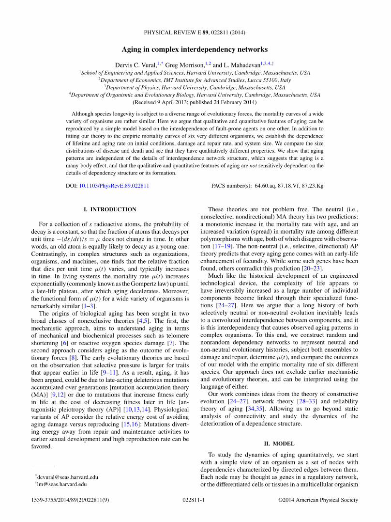
Typically, an organism starts its life with a slow decayof live cells φ at a rate of 〈a〉γ0, where the dimensionlessnumber 〈a〉 = 1.80 for scale-free networks and 〈a〉 = 1.75 forrandom networks. As an increasing number of nodes die, thesystem approaches a critical vitality φ(τ ) = φc when all livenodes suddenly collapse. Typical trajectories for both networktopologies as well as the values of 〈a〉 and φc are shown inFig. 1.

We observe that even if γ1 is set equal to γ0 the systemdecays steadily despite the seeming reversibility in dynamics.This is because while any live node can break, not all thedead nodes will have the sufficient number of live providers tosustain a repair.

022811-2

AGING IN COMPLEX INTERDEPENDENCY NETWORKS PHYSICAL REVIEW E 89, 022811 (2014)

τ

f(τ)

P(k) ~ k -3

P(k) ~ e-0.7 k

τ

f(τ)

Scale Free Networks Random Networks

0 20 40 60 800.0

0.2

0.4

0.6

0.8

1.0

t

φ

40 80 1200

0.25

0.5

0.75

0 20 40 60 80 100t

40 80 1200

0.25

0.5

0.75

FIG. 1. (Color online) Fraction φ(t) of live nodes, 100 runs.Dependency structures grown via non-neutral (left column) andneutral (right column) evolutionary schemes yield scale-free (SFN)and random degree (RN) distributions P (k). Although SFNs havehigh-degree hubs (black nodes) absent in RN, their aging character-istics share remarkable similarity. We plot 100 runs of φ(t) for eachnetwork size N and topology. Inset shows lifetime τ distributionsf (τ ). Increasing N = 2500 (light purple and pink) to N = 106 (darkblue and red) sharpens f (τ ). The black lines mark our theoreticalpredictions for initial slope p0 (=1.80γ0 for SFN and =1.75γ0 forRN) and critical fraction φc (=0.6 for SFN and =0.5 for RN), whichagree well with simulations. Here {γ0,γ1,d} = {0.0025,0,0}.

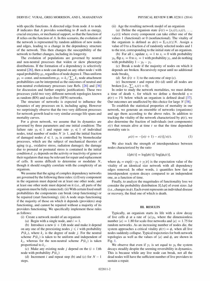
In Fig. 2 we quantitatively compare the mortality curvesgenerated by our digital populations to that of a variety oforganisms, C. elegans, drosophila, medflies, beetles, mice,Himalayan goats (Tahr), using data compiled from [1–3], andsee reasonable agreement between simulation and data.

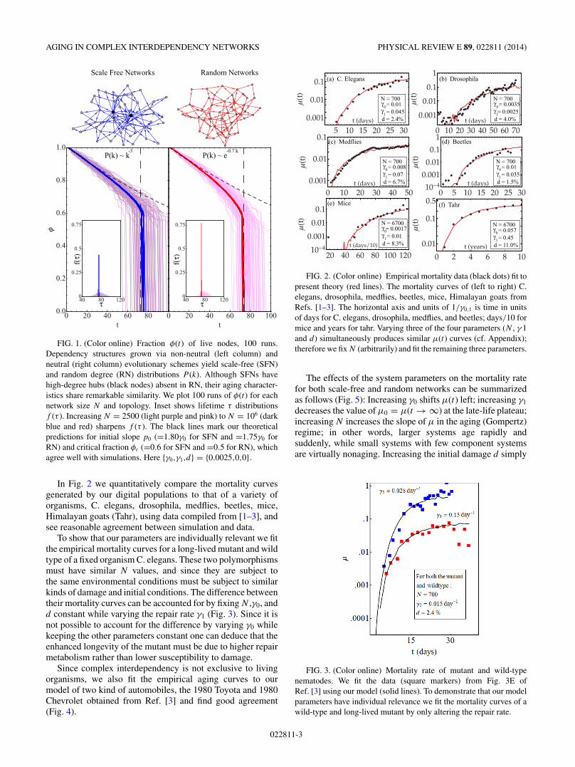
To show that our parameters are individually relevant we fitthe empirical mortality curves for a long-lived mutant and wildtype of a fixed organism C. elegans. These two polymorphismsmust have similar N values, and since they are subject tothe same environmental conditions must be subject to similarkinds of damage and initial conditions. The difference betweentheir mortality curves can be accounted for by fixing N ,γ0, andd constant while varying the repair rate γ1 (Fig. 3). Since it isnot possible to account for the difference by varying γ0 whilekeeping the other parameters constant one can deduce that theenhanced longevity of the mutant must be due to higher repairmetabolism rather than lower susceptibility to damage.

Since complex interdependency is not exclusive to livingorganisms, we also fit the empirical aging curves to ourmodel of two kind of automobiles, the 1980 Toyota and 1980Chevrolet obtained from Ref. [3] and find good agreement(Fig. 4).

0 2 4 6 8 10

0.01

0.1

0.5

μt

20 40 60 80 100 12010 4

0.001

0.01

0.1

μt

0 5 10 15 20 25 3010 4

0.001

0.01

0.1

1

μt

0 10 20 30 40 500.001

0.01

0.1

μt

0 10 20 30 40 50 60 70

0.001

0.01

0.1

1

μt

5 10 15 20 25 30

0.001

0.01

0.1

μt N = 700

γ0= 0.01

γ1= 0.045

d = 2.4%t (days)

(a) C. Elegans

N = 700γ

0= 0.0035γ

1= 0.0025d = 4.0%t (days)

(b) Drosophila

N = 700γ

0= 0.008γ

1= 0.07d = 6.7%t (days)

(c) Medflies

N = 700γ

0= 0.01γ

1= 0.035d = 1.5%t (days)

(d) Beetles

N = 6700γ

0= 0.0017γ

1= 0.01d = 8.3%t (days/10)

(e) Mice

N = 6700γ

0= 0.057γ

1= 0.45d = 11.0%t (years)

(f) Tahr

FIG. 2. (Color online) Empirical mortality data (black dots) fit topresent theory (red lines). The mortality curves of (left to right) C.elegans, drosophila, medflies, beetles, mice, Himalayan goats fromRefs. [1–3]. The horizontal axis and units of 1/γ0,1 is time in unitsof days for C. elegans, drosophila, medflies, and beetles; days/10 formice and years for tahr. Varying three of the four parameters (N , γ 1and d) simultaneously produces similar μ(t) curves (cf. Appendix);therefore we fix N (arbitrarily) and fit the remaining three parameters.

The effects of the system parameters on the mortality ratefor both scale-free and random networks can be summarizedas follows (Fig. 5): Increasing γ0 shifts μ(t) left; increasing γ1

decreases the value of μ0 = μ(t → ∞) at the late-life plateau;increasing N increases the slope of μ in the aging (Gompertz)regime; in other words, larger systems age rapidly andsuddenly, while small systems with few component systemsare virtually nonaging. Increasing the initial damage d simply

FIG. 3. (Color online) Mortality rate of mutant and wild-typenematodes. We fit the data (square markers) from Fig. 3E ofRef. [3] using our model (solid lines). To demonstrate that our modelparameters have individual relevance we fit the mortality curves of awild-type and long-lived mutant by only altering the repair rate.

022811-3

DERVIS C. VURAL, GREG MORRISON, AND L. MAHADEVAN PHYSICAL REVIEW E 89, 022811 (2014)

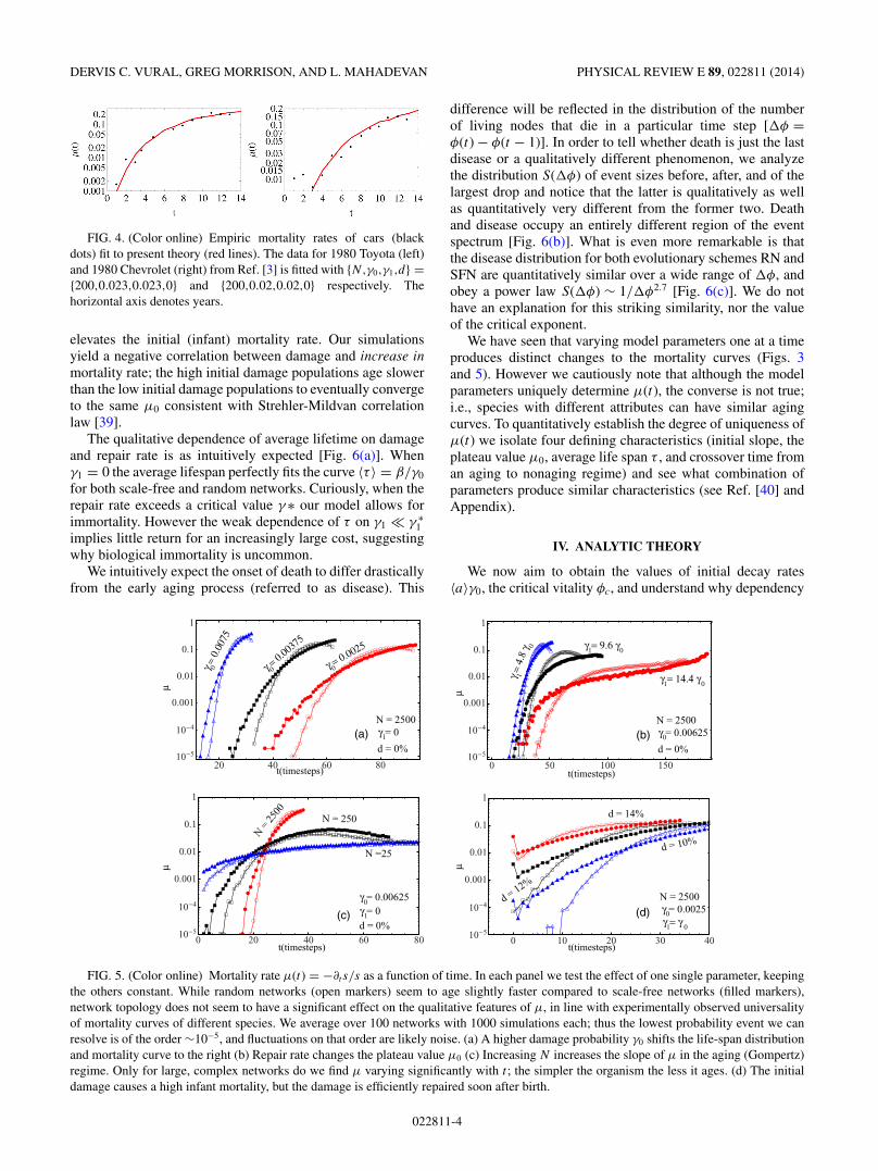
FIG. 4. (Color online) Empiric mortality rates of cars (blackdots) fit to present theory (red lines). The data for 1980 Toyota (left)and 1980 Chevrolet (right) from Ref. [3] is fitted with {N,γ0,γ1,d} ={200,0.023,0.023,0} and {200,0.02,0.02,0} respectively. Thehorizontal axis denotes years.

elevates the initial (infant) mortality rate. Our simulationsyield a negative correlation between damage and increase inmortality rate; the high initial damage populations age slowerthan the low initial damage populations to eventually convergeto the same μ0 consistent with Strehler-Mildvan correlationlaw [39].

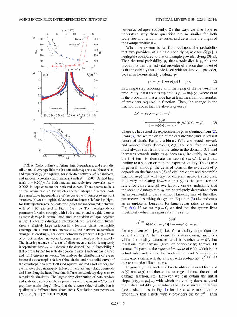
The qualitative dependence of average lifetime on damageand repair rate is as intuitively expected [Fig. 6(a)]. Whenγ1 = 0 the average lifespan perfectly fits the curve 〈τ 〉 = β/γ0

for both scale-free and random networks. Curiously, when therepair rate exceeds a critical value γ ∗ our model allows forimmortality. However the weak dependence of τ on γ1 � γ ∗

1implies little return for an increasingly large cost, suggestingwhy biological immortality is uncommon.

We intuitively expect the onset of death to differ drasticallyfrom the early aging process (referred to as disease). This

difference will be reflected in the distribution of the numberof living nodes that die in a particular time step [φ =φ(t) − φ(t − 1)]. In order to tell whether death is just the lastdisease or a qualitatively different phenomenon, we analyzethe distribution S(φ) of event sizes before, after, and of thelargest drop and notice that the latter is qualitatively as wellas quantitatively very different from the former two. Deathand disease occupy an entirely different region of the eventspectrum [Fig. 6(b)]. What is even more remarkable is thatthe disease distribution for both evolutionary schemes RN andSFN are quantitatively similar over a wide range of φ, andobey a power law S(φ) ∼ 1/φ2.7 [Fig. 6(c)]. We do nothave an explanation for this striking similarity, nor the valueof the critical exponent.

We have seen that varying model parameters one at a timeproduces distinct changes to the mortality curves (Figs. 3and 5). However we cautiously note that although the modelparameters uniquely determine μ(t), the converse is not true;i.e., species with different attributes can have similar agingcurves. To quantitatively establish the degree of uniqueness ofμ(t) we isolate four defining characteristics (initial slope, theplateau value μ0, average life span τ , and crossover time froman aging to nonaging regime) and see what combination ofparameters produce similar characteristics (see Ref. [40] andAppendix).

IV. ANALYTIC THEORY

We now aim to obtain the values of initial decay rates〈a〉γ0, the critical vitality φc, and understand why dependency

t(timesteps)

μ

0 50 100 15010 5

10 4

0.001

0.01

0.1

1

0 20 40 60 8010 5

10 4

0.001

0.01

0.1

1

t(timesteps)

μ

20 40 60 8010 5

10 4

0.001

0.01

0.1

1

t(timesteps)

μ

0 10 20 30 4010 5

10 4

0.001

0.01

0.1

1

t(timesteps)

μ

N = 2500γ = 0d = 0%

1

N = 2500γ = 0.00625d = 0%

0

γ = 0.00625

d = 0%

0γ = 01

N = 2500γ = 0.00250γ = γ 1 0

γ = 0.0025

0γ = 0.

0075

0 γ = 0.00375

0

γ = 4

.8 γ

1

0 γ = 9.6 γ 1 0

γ = 14.4 γ 1 0

N =25

N = 250

N = 25

00

d = 10%

d = 12%

d = 14%

(a) (b)

(c) (d)

FIG. 5. (Color online) Mortality rate μ(t) = −∂t s/s as a function of time. In each panel we test the effect of one single parameter, keepingthe others constant. While random networks (open markers) seem to age slightly faster compared to scale-free networks (filled markers),network topology does not seem to have a significant effect on the qualitative features of μ, in line with experimentally observed universalityof mortality curves of different species. We average over 100 networks with 1000 simulations each; thus the lowest probability event we canresolve is of the order ∼10−5, and fluctuations on that order are likely noise. (a) A higher damage probability γ0 shifts the life-span distributionand mortality curve to the right (b) Repair rate changes the plateau value μ0 (c) Increasing N increases the slope of μ in the aging (Gompertz)regime. Only for large, complex networks do we find μ varying significantly with t ; the simpler the organism the less it ages. (d) The initialdamage causes a high infant mortality, but the damage is efficiently repaired soon after birth.

022811-4

AGING IN COMPLEX INTERDEPENDENCY NETWORKS PHYSICAL REVIEW E 89, 022811 (2014)

0 10 20 30 40 50 60

1.0

1.5

2.0

2.5

3.0

3.5

t

λ(t) λ(φ)

0.5 0.6 0.7 0.8 0.9 1.0φ

Rando

m

Scale-Free

Disconnected

RandomScale-Free

Disconnected1.0

1.5

2.0

2.5

3.0

3.5

2 4 6 10 120

20

40

60

80

100

20 40 60 80 100 120

0

200

400

600

800

1000

γ0 (x 10 3)

τγ 0

γ1 x 10 3

τ(γ 1

)

Random

Scale-free

Varying γ0

Varying γ1

τ ∼ 0.2 / γ0

S(Δφ

)

Δφ

S(Δφ) ∼ Δφ −2.7

(a)

(b)

(c)

0.001 0.010 0.100 1.000

0.001

0.1

10 5

FIG. 6. (Color online) Lifetime, interdependence, and event dis-tribution. (a) Average lifetime 〈τ 〉 versus damage rate γ0 (blue circles)and repair rate γ1 (red squares) for scale-free networks (filled markers)and random networks (open markers) with N = 2500. Dashed linesmark τ = 0.20/γ0 for both random and scale-free networks. γ0 =0.0065 is kept constant for both red curves. There seems to be acritical repair rate γ ∗ for which expected lifespan diverges. Notethe remarkable independence of the curves with respect to networkstructure. (b) λ(t) = log[φ(t)]/γ0t as a function of t (left) and φ (right)for 100 trajectories on the scale-free (blue) and random (red) networkswith N = 106 pictured in Fig. 1 (γ1 = 0). The interdependenceparameter λ varies strongly with both t and φ, and roughly doublesas more damage is accumulated, until the sudden collapse depictedin Fig. 1 leads to a diverging interdependence. Scale-free networksshow a relatively large variation in λ for short times, but rapidlyconverge on a monotonic increase as the network accumulatesdamage. Interestingly, scale-free networks begin with a larger valueof λ, but random networks become more interdependent rapidly.The interdependence of a set of disconnected nodes (completelyindependent) have λ0 = 1 shown in the dashed line. (c) Probability S

that φ drops by φ for scale-free (open markers) and random (dashedand solid curves) networks. We analyze the distribution of eventsbefore the catastrophic failure (blue circles and blue solid curve) ofthe catastrophic failure itself (red squares and red short dashes) andevents after the catastrophic failure, if there are any (black diamondsand black long dashes). Note that different network topologies showremarkable similarity. The largest drop distribution of both randomand scale-free networks obey a power law with exponent −2.7, (thickgray line marks slope). Note that the disease (blue) distribution isqualitatively different from death (red). Simulation parameters are{N,γ0,γ1,d} = {2500,0.0025,0,0}.

networks collapse suddenly. On the way, we also hope tounderstand why these quantities are so similar for bothscale-free and random networks, and determine the origin ofthe Gompertz-like law.

When the system is far from collapse, the probabilitythat two providers of a single node dying at once O[γ 2

0 ] isnegligible compared to that of a single provider dying O[γ0].Then the total probability p0 that a node dies is γ0 plus theprobability that the last vital provider of a node dies. If m(φ)is the probability that a node is left with one last vital provider,we can self-consistently evaluate p0

p0 = γ0 + m(φ)p0(1 − γ0). (2)

In a single step associated with the aging of the network, theprobability that a node is repaired is p1 = h(φ)γ1, where h(φ)is the probability that a node has at least the minimum numberof providers required to function. Then, the change in thefraction of nodes that are alive is given by

φ = p0φ − p1(1 − φ)

= − γ0φ

1 − m(φ)(1 − γ0)+ γ1h(φ)(1 − φ), (3)

where we have used the expression for p0 as obtained from (2).From (3), we see the origin of the catastrophic (and universal)nature of death. For any arbitrary fully connected networkand monotonically decreasing φ(t), the vital fraction m(φ)must always start from a finite value in the domain [0,1] andincreases towards unity as φ decreases, inevitably to causethe first term to dominate the second (γ0 � 1), and thusleading to a sudden drop in the expected vitality. This is truein general, although the detailed form of the evolution of φ

depends on the fraction m(φ) of vital providers and repairablefraction h(φ) that will vary for different network structures.It is very interesting however, that γ0 is the same for thereference curve and all overlapping curves, indicating thatthe somatic damage rate γ0 can be uniquely determined froman experimental μ curve without knowing any of the otherparameters describing the system. Equation (3) also indicatesan asymptote in longevity for large repair rates, as seen inFig. 6(a). If we set φ = 0, we find that the system livesindefinitely when the repair rate γ1 is set to

γ ∗1 = γ0φ

∗

h(φ∗)(1 − φ∗)[1 − m(φ∗)(1 − γ0)]

for any given φ∗ ∈ [φc,1], i.e., for a vitality larger than thecritical vitality φc. In this case the system damage increaseswhile the vitality decreases until it reaches φ = φ∗, butmaintains that damage (level of connectivity) forever. Ofcourse, (3) governs the expectation value of φ(t), which is theactual value only in the thermodynamic limit N → ∞; anyfinite-size system will die at least with probability γ

N(φ(t)−φc)0

due to statistical fluctuations.In general, it is a nontrivial task to obtain the exact forms of

m(φ) and h(φ) and thence the average lifetime, the criticaldamage fraction, etc. However we can obtain the initialslope 〈a〉γ0 = p0|t=0 with which the vitality decreases, andthe critical vitality φc at which the whole system collapses(see dashed lines in Fig. 1) for the case γ1 = 0: Let theprobability that a node with k providers die be σ (k). Then

022811-5

DERVIS C. VURAL, GREG MORRISON, AND L. MAHADEVAN PHYSICAL REVIEW E 89, 022811 (2014)

we can recursively obtain σ (1) in terms of the others [41],

σ (1) = γ0 + P (1,1)σ (1) + P (1,2)σ (2) + P (1,3)σ (3) + · · · ,

(4)

where P (1,i) is the probability that a node is provided byone other node, and that the provider itself has i providers.The first term corresponds to the probability that a node diesindependent of its connectivity.

Since we neglect probabilities of order O[γ 20 ], initially only

degree-1 nodes can be killed by the death of their providers.Thus substituting σ (k) = γ0 for all k apart from k = 1, andusing

∑i P (1,i) = P (1) we can obtain from (4) the initial

probability that a degree-1 node dies,

σ (1) = (2 − P (1,1))γ0

1 − P (1,1). (5)

To find the expectation value of the initial slope we mustaverage over the damage rate of all degrees, including σ (k) =γ0 for k > 1

〈a〉γ0 =∑

k

P (k)σ (k)

∣∣∣∣∣t=0

= γ0

(1 + P (1)

1 − P (1,1)

). (6)

Upon substituting the numerical values of P (1) and P (1,1) forthe networks we evolved, we obtain 〈a〉 = 1.75 for the neutralscheme and 〈a〉 = 1.80 for non-neutral scheme, i.e., only a∼2.8% difference between two topologies. These initial slopesare consistent with our aging simulations (Fig. 1).

To heuristically estimate the critical vitality φc, we supposethat there exists a unique value of φc regardless of the historyof the network. If so, then the collapse can occur not only ifφ approaches φc in τ steps, it can also occur in precisely onestep due to a larger damage, γ0c = 1 − φc. Thus if we substituteγ0 → 1 − φc in (4) and let σ (i) → 1 for all i to obtain a simplebut interesting result,

φc = P (1).

For the networks we evolved, P (1) is 0.5 for the neutral schemeand 0.6 for the non-neutral scheme. These values are consistentwith the critical vitalities we observed in our aging simulations(Fig. 1).

Having estimated the average damage rate and the criticalvitality of the network, we now consider the nature of life-spandistributions. The probability of network survival s(t) is equalto the probability of δφ being not greater than φ − φc. Sinceeach node dies with probability p0,

s(t) = 1 − Prob(φ > φ − φc)

= 1 −Nφc∑k=0

(Nφ

N (φ − φc) + k

)p

N(φ−φc)+k

0 (1 − p0)Nφc−k.

(7)

Since 1.75γ0 < p0 < 1 is a constant, in the limit N → ∞the probability of death 1 − s(t) simply becomes a unit stepfunction. On the other hand for finite N , the step functionsoftens, and we empirically interpret the rapid transitionfrom s = 1 to s = 0 as aging. We see that by passing fromfinite size to infinite size, we also pass from the stochastic todeterministic, and from gradual slow aging to instant aging.

Finally, we consider the sharpness of the transition froms = 1 to s = 0 to see if there is any relation between our resultsand the classical Gompertz law for mortality. An approximateevaluation of (7) is carried out and plotted in the Appendix.

V. DISCUSSION

We have built on a similarity between large networks andcomplex organisms (and machines) to create a minimal modelfor how large networks (and thence organisms or machines)might age. It is thus important to be self-critical here bycomparing our study both with reality and with previousattempts. Any theory that aims to account for a phenomenonas universal as aging, spanning both animate and inanimateobjects, needs to be robust, i.e., it should not have such strongassumptions and results that sensitively depend on it. Theweak sensitivity of our outcomes to the details of biologicallyjustifiable dependency network structures (Figs. 1–6) seems tosatisfy this requirement.

Our analysis differs significantly from earlier theoreticalinvestigations of network failure [29–32] in which nodes aresimply removed one by one (systematically or randomly)until networks get fragmented. In these approaches the nodesdo not influence the performance of one other, and are notallowed to be repaired. Curiously, the lack of interactions inthese models leads to fundamentally different fragmentationdynamics in scale-free and random networks. In contrast,the survival curves we observe are remarkably independentof the network topology (cf. Figs. 1, 5, and 6). The stronginteractions between components may indeed be the reasonbehind the strong similarity of mortality curves among so manyorganisms. Indeed, this is also consistent with a class of modelsthat do account for strong interactions, though very differentlythan ours, and have been proposed to explain electrical girdfailures [32]. Much still remains to be done in understandinghow the form of these interactions leads to differences orsimilarities in the dynamics.

Our study has focused on the dynamics of networks that ageas a consequence of increasing interdependency, and thus leadsnaturally to the question of how this might be controlled. Sincethe repair rate, and perhaps the damage rate (to a lesser extent)are experimentally controllable, one might ask if it is possibleto vary their temporal character while keeping their averageconstant. Are there optimal strategies for repair—either in thetime domain or in space (i.e., looking at nodes with varyingconnectivity)? For example, Fig. 6(a) shows that if the systemis repaired uniformly, the degree of repair does not make asignificant difference for γ1 < γ ∗

1 . It would be very useful toknow if and how a (temporal or spatial) nonuniform repairstrategy improves life span. In networks that are dynamicallyheterogeneous, we may ask what would be the consequencesof differential damage and repair in a network with highlyvariable turnover, e.g., a network with tissues like the skin orgut that have high damage and repair rates, and the brain whichhas a low damage and repair rate? At the level of ecologiesand colonies, we might ask how does the aging dynamics of adependency network change when a system consists of partswith aging rates comparable to that of the whole system? Wehope that our minimal model may be used to study some ofthese questions.

022811-6

AGING IN COMPLEX INTERDEPENDENCY NETWORKS PHYSICAL REVIEW E 89, 022811 (2014)

40 50 60 70 80 90 10010 16

10 13

10 10

10 7

10 4

0.1

t

μt

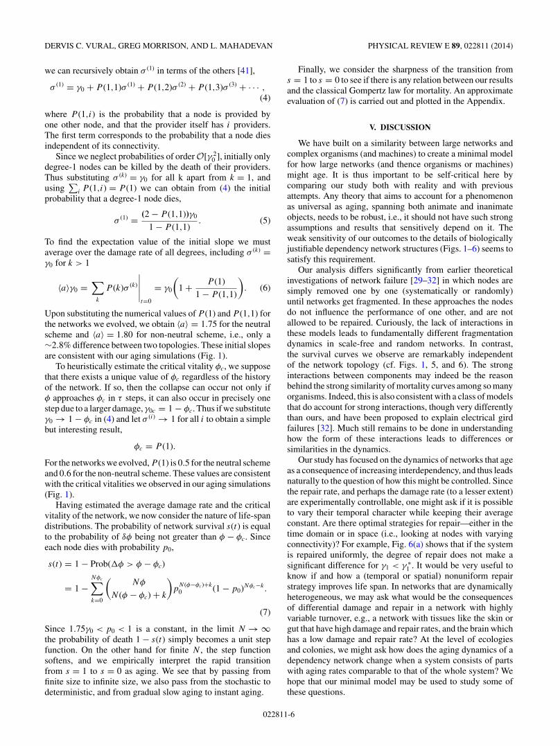
FIG. 7. (Color online) Mortality vs time obtained from (7) forφ � φc, γ0 = 0.0025 and N = 50 (black, left) 100 (red, middle), and200 (blue, right) is in good qualitative agreement with our simulationsand the empiric Gompertz law, which states that log μ(t) increaseslinearly with t early in life.

ACKNOWLEDGMENTS

D.C.V. thanks Anthony J. Leggett for his support, andthanks Pinar Zorlutuna for many stimulating discussions. Thiswork was partly supported by NSF Grants No. NSF-DMR-03-50842, and No. NSF-DMR09-06921, the Wyss Institute forBiologically Inspired Engineering, the Harvard Kavli Institutefor Bio-nano Science and Technology, and the MacArthurFoundation.

APPENDIX

Here we discuss various technical points surroundingtheory, simulations, and fits.

(i) In order to recover the Gompertz Law analytically,we substitute φ(t) ≈ e−aγ0t for t � τ in (7) and plotμ(t) = −(ds(t)/dt)/s(t) in Fig. 7. By approximating therandom variables φ(t) and p0 by their average value wesharpen the lifetime distributions and hence steepen themortality curve; however the qualitative features of μ(t) isrecovered.

(ii) We have defined death as the time τ at which φ

reaches a threshold value 1%, which may seem arbitrary.

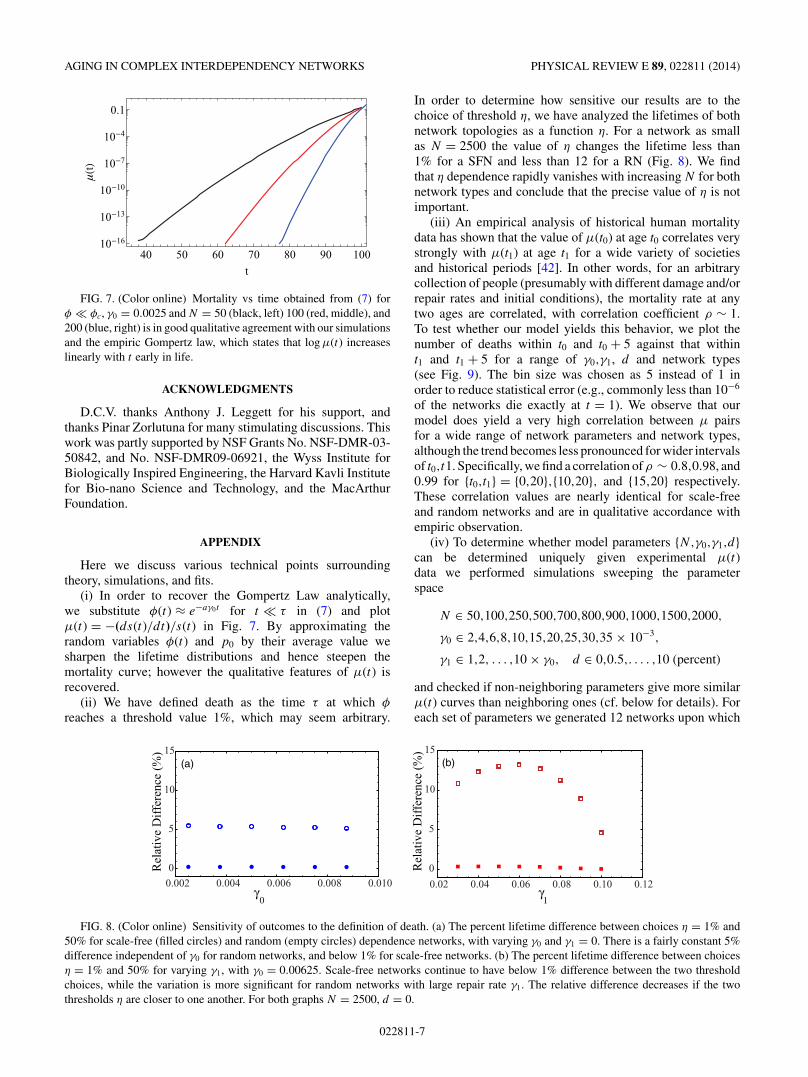
In order to determine how sensitive our results are to thechoice of threshold η, we have analyzed the lifetimes of bothnetwork topologies as a function η. For a network as smallas N = 2500 the value of η changes the lifetime less than1% for a SFN and less than 12 for a RN (Fig. 8). We findthat η dependence rapidly vanishes with increasing N for bothnetwork types and conclude that the precise value of η is notimportant.

(iii) An empirical analysis of historical human mortalitydata has shown that the value of μ(t0) at age t0 correlates verystrongly with μ(t1) at age t1 for a wide variety of societiesand historical periods [42]. In other words, for an arbitrarycollection of people (presumably with different damage and/orrepair rates and initial conditions), the mortality rate at anytwo ages are correlated, with correlation coefficient ρ ∼ 1.To test whether our model yields this behavior, we plot thenumber of deaths within t0 and t0 + 5 against that withint1 and t1 + 5 for a range of γ0,γ1, d and network types(see Fig. 9). The bin size was chosen as 5 instead of 1 inorder to reduce statistical error (e.g., commonly less than 10−6

of the networks die exactly at t = 1). We observe that ourmodel does yield a very high correlation between μ pairsfor a wide range of network parameters and network types,although the trend becomes less pronounced for wider intervalsof t0,t1. Specifically, we find a correlation of ρ ∼ 0.8,0.98, and0.99 for {t0,t1} = {0,20},{10,20}, and {15,20} respectively.These correlation values are nearly identical for scale-freeand random networks and are in qualitative accordance withempiric observation.

(iv) To determine whether model parameters {N,γ0,γ1,d}can be determined uniquely given experimental μ(t)data we performed simulations sweeping the parameterspace

N ∈ 50,100,250,500,700,800,900,1000,1500,2000,

γ0 ∈ 2,4,6,8,10,15,20,25,30,35 × 10−3,

γ1 ∈ 1,2, . . . ,10 × γ0, d ∈ 0,0.5,. . . . ,10 (percent)

and checked if non-neighboring parameters give more similarμ(t) curves than neighboring ones (cf. below for details). Foreach set of parameters we generated 12 networks upon which

0.002 0.004 0.006 0.008 0.010

0

5

10

15

0.02 0.04 0.06 0.08 0.10 0.12

0

5

10

15

Rel

ativ

e D

iffer

ence

(%)

γγ10

Rel

ativ

e D

iffer

ence

(%)

(a) (b)

FIG. 8. (Color online) Sensitivity of outcomes to the definition of death. (a) The percent lifetime difference between choices η = 1% and50% for scale-free (filled circles) and random (empty circles) dependence networks, with varying γ0 and γ1 = 0. There is a fairly constant 5%difference independent of γ0 for random networks, and below 1% for scale-free networks. (b) The percent lifetime difference between choicesη = 1% and 50% for varying γ1, with γ0 = 0.00625. Scale-free networks continue to have below 1% difference between the two thresholdchoices, while the variation is more significant for random networks with large repair rate γ1. The relative difference decreases if the twothresholds η are closer to one another. For both graphs N = 2500, d = 0.

022811-7

DERVIS C. VURAL, GREG MORRISON, AND L. MAHADEVAN PHYSICAL REVIEW E 89, 022811 (2014)

0.200.15

0.50

0.30

μcoarse 3

μ coa

rse

5

0.20 0.30

0.50

0.30

μcoarse 4

μ coa

rse

5

0.010 0.020 0.0300.015

0.50

0.30

μcoarse 1

μ coa

rse

5

0 10 20 30 4010 5

10 4

0.001

0.01

0.1

1

t

μt

0 10 20 30 40

0.001

0.01

0.1

1

t

μt

(a) (b) (c)

(d) (e)

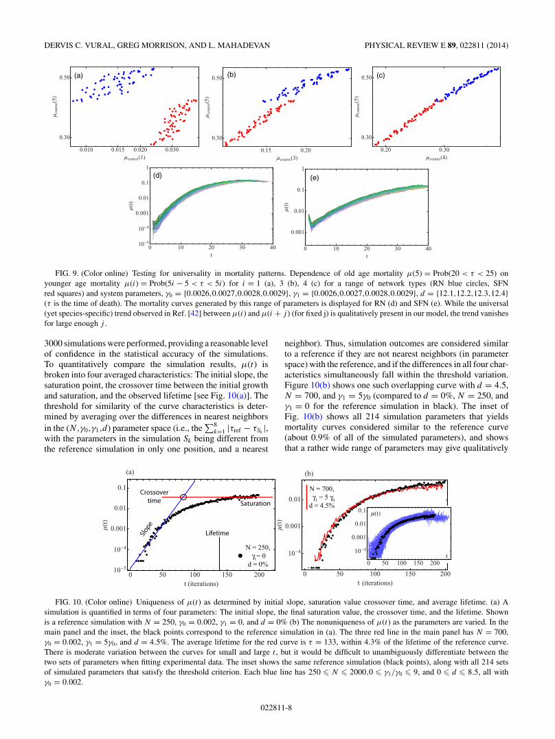
FIG. 9. (Color online) Testing for universality in mortality patterns. Dependence of old age mortality μ(5) = Prob(20 < τ < 25) onyounger age mortality μ(i) = Prob(5i − 5 < τ < 5i) for i = 1 (a), 3 (b), 4 (c) for a range of network types (RN blue circles, SFNred squares) and system parameters, γ0 = {0.0026,0.0027,0.0028,0.0029}, γ1 = {0.0026,0.0027,0.0028,0.0029}, d = {12.1,12.2,12.3,12.4}(τ is the time of death). The mortality curves generated by this range of parameters is displayed for RN (d) and SFN (e). While the universal(yet species-specific) trend observed in Ref. [42] between μ(i) and μ(i + j ) (for fixed j) is qualitatively present in our model, the trend vanishesfor large enough j .

3000 simulations were performed, providing a reasonable levelof confidence in the statistical accuracy of the simulations.To quantitatively compare the simulation results, μ(t) isbroken into four averaged characteristics: The initial slope, thesaturation point, the crossover time between the initial growthand saturation, and the observed lifetime [see Fig. 10(a)]. Thethreshold for similarity of the curve characteristics is deter-mined by averaging over the differences in nearest neighborsin the (N,γ0,γ1,d) parameter space (i.e., the

∑8k=1 |τref − τSk

|,with the parameters in the simulation Sk being different fromthe reference simulation in only one position, and a nearest

neighbor). Thus, simulation outcomes are considered similarto a reference if they are not nearest neighbors (in parameterspace) with the reference, and if the differences in all four char-acteristics simultaneously fall within the threshold variation.Figure 10(b) shows one such overlapping curve with d = 4.5,N = 700, and γ1 = 5γ0 (compared to d = 0%, N = 250, andγ1 = 0 for the reference simulation in black). The inset ofFig. 10(b) shows all 214 simulation parameters that yieldsmortality curves considered similar to the reference curve(about 0.9% of all of the simulated parameters), and showsthat a rather wide range of parameters may give qualitatively

N = 700, γ = 5 γ

d = 4.5%1 0

(a) (b)

Slope

Saturation

Crossovertime

Lifetime

0 50 100 150 20010 5

10 4

0.001

0.01

0.1

t (iterations)

μt

0 50 100 150 200

10 4

0.001

0.01

t

μt

(iterations)

N = 250, γ = 0

d = 0%1

0 50 100 150 200

10 4

0.001

0.01

0.1

t

μ t

FIG. 10. (Color online) Uniqueness of μ(t) as determined by initial slope, saturation value crossover time, and average lifetime. (a) Asimulation is quantified in terms of four parameters: The initial slope, the final saturation value, the crossover time, and the lifetime. Shownis a reference simulation with N = 250, γ0 = 0.002, γ1 = 0, and d = 0% (b) The nonuniqueness of μ(t) as the parameters are varied. In themain panel and the inset, the black points correspond to the reference simulation in (a). The three red line in the main panel has N = 700,γ0 = 0.002, γ1 = 5γ0, and d = 4.5%. The average lifetime for the red curve is τ = 133, within 4.3% of the lifetime of the reference curve.There is moderate variation between the curves for small and large t , but it would be difficult to unambiguously differentiate between thetwo sets of parameters when fitting experimental data. The inset shows the same reference simulation (black points), along with all 214 setsof simulated parameters that satisfy the threshold criterion. Each blue line has 250 � N � 2000,0 � γ1/γ0 � 9, and 0 � d � 8.5, all withγ0 = 0.002.

022811-8

AGING IN COMPLEX INTERDEPENDENCY NETWORKS PHYSICAL REVIEW E 89, 022811 (2014)

similar behavior in μ and τ (with the latter not shown). Itis interesting to note that γ0 is the same for the reference

curve and all overlapping curves, indicating that an empiricallyobserved death rate γ0 may be uniquely determined.

[1] S. Horiuchi, Pop. Dev. Rev. 29, 127 (2003).[2] G. Caughley, Ecology 47, 906 (1966).[3] J. W. Vaupel, J. R. Carey, K. Christensen, T. E. Johnson, A. I.

Yashin et al., Science 280, 855 (1998).[4] K. A. Highes and R. M. Raynolds, Ann. Rev. Entomol. 50, 421

(2005).[5] B. T. Weinert and P. S. Timiras, J. Appl. Physiol. 95, 1706

(2003).[6] E. H. Blackburn, Nature (London) 408, 53 (2000).[7] D. Harman, J. Gerontol. 2, 298 (1957).[8] A. Baudisch, Gerontology 58, 481 (2012).[9] P. B. Medawar, An unsolved problem in biology (H. K. Lewis &

Co., London, 1952).[10] G. C. Williams, Evolution 11, 398 (1957).[11] W. D. Hamilton, J. Theor. Biol. 12, 12 (1966).[12] P. B. Medawar, Mod. Quart. 1, 30 (1946).[13] M. R. Rose, Evolutionary Biology of Aging (Oxford University

Press, New York, 1991).[14] T. B. L. Kirkwood, Mech. Aging Dev. 123, 737 (2002).[15] T. B. L. Kirkwood, Nature (London) 270, 301 (1977).[16] P. A. Abrams and D. Ludwig, Evolution 49, 1055 (1995).[17] J. W. Curtsinger, H. H. Fukui, D. R. Townsend, and J. W. Vaupel,

Science 258, 461 (1992).[18] J. R. Carey, P. Liedo, D. Orozco, and J. W. Vaupel, Science 258,

457 (1992).[19] D. E. L. Promislow, M. Tatar, A. A. Khazaeli, and J. W.

Curtsinger, Genetics 143, 839 (1996).[20] D. A. Gray and W. H. Cade, Can. J. Zool. 78, 140

(2000).[21] R. A. Miller, R. Dysko, C. Chrisp, R. Seguin, L. Linsalata et al.,

J. Zool. 250, 95 (2000).[22] R. A. Miller, J. M. Harper, R. C. Dysko, S. J. Durkee, and S. N.

Austad, Exp. Biol. Med. 227, 500 (2002).[23] D. Reznick, G. Buckwalter, J. Groff, and D. Elder,

Exp. Gerontol. 36, 791 (2001).[24] M. W. Gray, J. Lukes, J. M. Archibald, P. J. Keeling, and

W. Doolittle, Science 330, 920 (2010).[25] M. Lynch, Proc. Natl. Acad. Sci. USA 104, 8597 (2007).[26] A. Stoltzfus, J. Mol. Evol. 49, 169 (1999).[27] H. J. M. Kiss, A. Mihalik, T. Nanasi, B. Ory, Z. Spiro, C. Soti,

and P. Csermely, BioEssays 31, 651 (2009).[28] M. Scheffer, J. Bascompte, W. A. Brock, V. Brokvin, S. R.

Carpenter et al., Nature (London) 461, 53 (2009).[29] R. Albert, H. Jeong, and A. L. Barabasi, Nature (London) 406,

378 (2000).

[30] T. Tanizawa, G. Paul, R. Cohen, S. Havlin, and H. E. Stanley,Phys. Rev. E 71, 047101 (2005).

[31] R. Cohen, D. ben-Avraham, and S. Havlin, Phys. Rev. E 66,036113 (2002).

[32] S. V. Buldyrev, R. Parshani, G. Paul, H. E. Stanley, andS. Havlin, Nature (London) 464, 1025 (2010).

[33] G. I. Simko, D. Gyurko, D. V. Veres, T. Nanasi, and P. Csermely,Genome Med. 1, 90 (2009).

[34] L. A. Gavrilov and N. S. Gavrilova, J. Theor. Biol. 213, 527(2001).

[35] R. A. Laird and T. N. Sherratt, J. Evol. Biol. 22, 974 (2009).[36] H. Jeong, B. Tombor, R. Albert, Z. N. Oltvai, and A. L. Barabasi,

Nature (London) 407, 651 (2000).[37] For two other choices (τ0, the time at which no nodes are left

alive, or τm, the time at which the largest drop in φ occurs), wehave τ0 ≈ τm ≈ τ for large N. We find that in smaller networks(particularly RN) these times may differ. Interestingly τ is notalways well defined in nature either; for example, parts ofcockroaches are known to survive for weeks after the insectis decapitated [43].

[38] In order to determine how sensitive our results are to thechoice of threshold η, we have analyzed the lifetimes of bothnetwork topologies as a function η. For a network as smallas N = 2500, the choice of η changes the lifetime by ∼1%for a SFN and ∼%10 for a RN. We find that for N > O [106]the η dependence practically vanishes for both network types.We therefore conclude that the precise value of η is notimportant.

[39] B. L. Strehler and A. S. Mildvan, Science 132, 14 (1960).[40] The threshold for similarity of the curve characteristics is de-

termined by averaging over the differences in nearest neighborsin the (N,γ0,γ1,d) parameter space (i.e., the

∑8k=1 |τref − τSk

|,with the parameters in the simulation Sk being different fromthe reference simulation in only one position, and a nearestneighbor). Thus, simulation outcomes are considered similar toa reference if they are not nearest neighbors (in parameter space)with the reference, and if the differences in all four characteris-tics simultaneously fall within the threshold variation.

[41] Analogous equations can be written for σ (i) for i > 1; howeverthese equations will depend on P (i; x1x2 . . . xi), the probabilitythat a node with i providers has one provider with x1 providers,one provider with x2 providers, and so on. Fortunately we donot need these equations to obtain φc and a.

[42] M. Ya. Azbel, Phys. Rev. E 66, 016107 (2002).[43] C. Q. Choi, Sci. Am. 297, 116 (2007).

022811-9