1

AI-IMU Dead-ReckoningMartin BROSSARD∗ , Axel BARRAU† and Silvere BONNABEL∗

∗MINES ParisTech, PSL Research University, Centre for Robotics, 60 Bd Saint-Michel, 75006 Paris, France†Safran Tech, Groupe Safran, Rue des Jeunes Bois-Chateaufort, 78772, Magny Les Hameaux Cedex, France

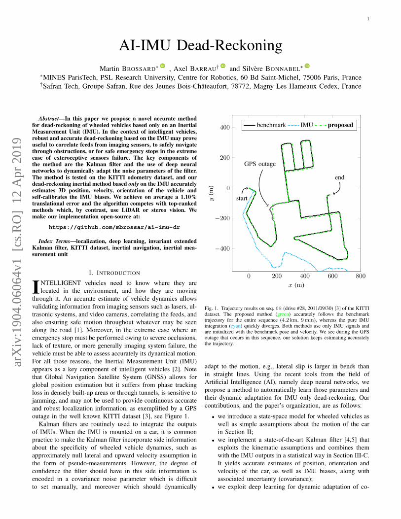
Abstract—In this paper we propose a novel accurate methodfor dead-reckoning of wheeled vehicles based only on an InertialMeasurement Unit (IMU). In the context of intelligent vehicles,robust and accurate dead-reckoning based on the IMU may proveuseful to correlate feeds from imaging sensors, to safely navigatethrough obstructions, or for safe emergency stops in the extremecase of exteroceptive sensors failure. The key components ofthe method are the Kalman filter and the use of deep neuralnetworks to dynamically adapt the noise parameters of the filter.The method is tested on the KITTI odometry dataset, and ourdead-reckoning inertial method based only on the IMU accuratelyestimates 3D position, velocity, orientation of the vehicle andself-calibrates the IMU biases. We achieve on average a 1.10%translational error and the algorithm competes with top-rankedmethods which, by contrast, use LiDAR or stereo vision. Wemake our implementation open-source at:

https://github.com/mbrossar/ai-imu-dr

Index Terms—localization, deep learning, invariant extendedKalman filter, KITTI dataset, inertial navigation, inertial mea-surement unit

I. INTRODUCTION

INTELLIGENT vehicles need to know where they arelocated in the environment, and how they are moving

through it. An accurate estimate of vehicle dynamics allowsvalidating information from imaging sensors such as lasers, ul-trasonic systems, and video cameras, correlating the feeds, andalso ensuring safe motion throughout whatever may be seenalong the road [1]. Moreover, in the extreme case where anemergency stop must be performed owing to severe occlusions,lack of texture, or more generally imaging system failure, thevehicle must be able to assess accurately its dynamical motion.For all those reasons, the Inertial Measurement Unit (IMU)appears as a key component of intelligent vehicles [2]. Notethat Global Navigation Satellite System (GNSS) allows forglobal position estimation but it suffers from phase trackingloss in densely built-up areas or through tunnels, is sensitive tojamming, and may not be used to provide continuous accurateand robust localization information, as exemplified by a GPSoutage in the well known KITTI dataset [3], see Figure 1.

Kalman filters are routinely used to integrate the outputsof IMUs. When the IMU is mounted on a car, it is commonpractice to make the Kalman filter incorporate side informationabout the specificity of wheeled vehicle dynamics, such asapproximately null lateral and upward velocity assumption inthe form of pseudo-measurements. However, the degree ofconfidence the filter should have in this side information isencoded in a covariance noise parameter which is difficultto set manually, and moreover which should dynamically

0 200 400 600 800

−400

−200

0

200

400

start

GPS outage

end

x (m)

y(m

)

benchmark IMU proposed

Fig. 1. Trajectory results on seq. 08 (drive #28, 2011/09/30) [3] of the KITTIdataset. The proposed method (green) accurately follows the benchmarktrajectory for the entire sequence (4.2 km, 9min), whereas the pure IMUintegration (cyan) quickly diverges. Both methods use only IMU signals andare initialized with the benchmark pose and velocity. We see during the GPSoutage that occurs in this sequence, our solution keeps estimating accuratelythe trajectory.

adapt to the motion, e.g., lateral slip is larger in bends thanin straight lines. Using the recent tools from the field ofArtificial Intelligence (AI), namely deep neural networks, wepropose a method to automatically learn those parameters andtheir dynamic adaptation for IMU only dead-reckoning. Ourcontributions, and the paper’s organization, are as follows:

• we introduce a state-space model for wheeled vehicles aswell as simple assumptions about the motion of the carin Section II;

• we implement a state-of-the-art Kalman filter [4,5] thatexploits the kinematic assumptions and combines themwith the IMU outputs in a statistical way in Section III-C.It yields accurate estimates of position, orientation andvelocity of the car, as well as IMU biases, along withassociated uncertainty (covariance);

• we exploit deep learning for dynamic adaptation of co-

arX

iv:1

904.

0606

4v1

[cs

.RO

] 1

2 A

pr 2

019

2

variance noise parameters of the Kalman filter in SectionIV-A. This module greatly improves filter’s robustnessand accuracy, see Section V-D;

• we demonstrate the performances of the approach on theKITTI dataset [3] in Section V. Our approach solelybased on the IMU produces accurate estimates and com-petes with top-ranked LiDAR and stereo camera methods[6,7]; and we do not know of IMU based dead-reckoningmethods capable to compete with such results;

• the approach is not restricted to inertial only dead-reckoning of wheeled vehicles. Thanks to the versatilityof the Kalman filter, it can easily be applied for railwayvehicles [8], coupled with GNSS, the backbone for IMUself-calibration, or for using IMU as a speedometer inpath-reconstruction and map-matching methods [9]–[12].

A. Relation to Previous Literature

Autonomous vehicle must robustly self-localize with theirembarked sensor suite which generally consists of odometers,IMUs, radars or LiDARs, and cameras [1,2,12]. SimultaneousLocalization And Mapping based on inertial sensors, cameras,and/or LiDARs have enabled robust real-time localization sys-tems, see e.g., [6,7]. Although these highly accurate solutionsbased on those sensors have recently emerged, they may driftwhen the imaging system encounters troubles.

As concerns wheeled vehicles, taking into account vehicleconstraints and odometer measurements are known to increasethe robustness of localization systems [13]–[16]. Althoughquite successful, such systems continuously process a largeamount of data which is computationally demanding andenergy consuming. Moreover, an autonomous vehicle shouldrun in parallel its own robust IMU-based localization algorithmto perform maneuvers such as emergency stops in case of othersensors failures, or as an aid for correlation and interpretationof image feeds [2].

High precision aerial or military inertial navigation systemsachieve very small localization errors but are too costly forconsumer vehicles. By contrast, low and medium-cost IMUssuffer from errors such as scale factor, axis misalignment andrandom walk noise, resulting in rapid localization drift [17].This makes the IMU-based positioning unsuitable, even duringshort periods.

Inertial navigation systems have long leveraged virtual andpseudo-measurements from IMU signals, e.g. the widespreadZero velocity UPdaTe (ZUPT) [18]–[20], as covariance adap-tation [21]. In parallel, deep learning and more generally ma-chine learning are gaining much interest for inertial navigation[22,23]. In [22] velocity is estimated using support vectorregression whereas [23] use recurrent neural networks for end-to-end inertial navigation. Those methods are promising butrestricted to pedestrian dead-reckoning since they generallyconsider slow horizontal planar motion, and must infer ve-locity directly from a small sequence of IMU measurements,whereas we can afford to use larger sequences. A moregeneral end-to-end learning approach is [24], which trainsdeep networks end-to-end in a Kalman filter. Albeit promising,the method obtains large translational error > 30% in their

stereo odometry experiment. Finally, [25] uses deep learningfor estimating covariance of a local odometry algorithm thatis fed into a global optimization procedure, and in [26] weused Gaussian processes to learn a wheel encoders error. Ourconference paper [20] contains preliminary ideas, albeit notconcerned at all with covariance adaptation: a neural networkessentially tries to detect when to perform ZUPT.

Dynamic adaptation of noise parameters in the Kalman filteris standard in the tracking literature [27], however adaptationrules are application dependent and are generally the resultof manual “tweaking” by engineers. Finally, in [28] theauthors propose to use classical machine learning techniquesto to learn static noise parameters (without adaptation) of theKalman filter, and apply it to the problem of IMU-GNSSfusion.

II. IMU AND PROBLEM MODELLING

An inertial navigation system uses accelerometers and gyrosprovided by the IMU to track the orientation Rn, velocityvn ∈ R3 and position pn ∈ R3 of a moving platform relativeto a starting configuration (R0,v0,p0). The orientation isencoded in a rotation matrix Rn ∈ SO(3) whose columnsare the axes of a frame attached to the vehicle.

A. IMU Modelling

The IMU provides noisy and biased measurements of theinstantaneous angular velocity vector ωn and specific acceler-ation an as follows [17]

ωIMUn = ωn + bωn +wωn , (1)

aIMUn = an + ba

n +wan, (2)

where bωn , ban are quasi-constant biases and wωn , wa

n are zero-mean Gaussian noises. The biases follow a random walk

bωn+1 = bωn +wbωn , (3)

ban+1 = ba

n +wban , (4)

where wbωn , wba

n are zero-mean Gaussian noises.The kinematic model is governed by the following equations

RIMUn+1 = RIMU

n exp ((ωndt)×) , (5)vIMUn+1 = vIMU

n + (RIMUn an + g) dt, (6)

pIMUn+1 = pIMU

n + vIMUn dt, (7)

between two discrete time instants sampling at dt, where welet the IMU velocity be vIMU

n ∈ R3 and its position pIMUn ∈ R3

in the world frame. RIMUn ∈ SO(3) is the 3×3 rotation matrix

that represents the IMU orientation, i.e. that maps the IMUframe to the world frame, see Figure 2. Finally (y)× denotesthe skew symmetric matrix associated with cross product withy ∈ R3. The true angular velocity ωn ∈ R3 and the truespecific acceleration an ∈ R3 are the inputs of the system (5)-(7). In our application scenarios, the effects of earth rotationand Coriolis acceleration are ignored, Earth is considered flat,and the gravity vector g ∈ R3 is a known constant.

All sources of error displayed in (1) and (2) are harmfulsince a simple implementation of (5)-(7) leads to a tripleintegration of raw data, which is much more harmful that the

3

w

c

◦ i

◦

RIMUn ,pIMU

n

vcn

Rcn,p

cn

vIMUn

Fig. 2. The coordinate systems that are used in the paper. The IMU pose(RIMU

n ,pIMUn ) maps vectors expressed in the IMU frame i (red) to the world

frame w (black). The IMU frame is attached to the vehicle and misaligned withthe car frame c (blue). The pose between the car and inertial frames (Rc

n,pcn)

is unknown. IMU velocity vIMUn and car velocity vc

n are respectively expressedin the world frame and in the car frame.

unique integration of differential wheel speeds [12]. Indeed, abias of order ε has an impact of order εt2/2 on the positionafter t seconds, leading to potentially huge drift.

B. Problem ModellingWe distinguish between three different frames, see Figure 2:

i) the static world frame, w; ii) the IMU frame, i, where (1)-(2) are measured; and iii) the car frame, c. The car frame is anideal frame attached to the car, that will be estimated onlineand plays a key role in our approach. Its orientation w.r.t. i isdenoted Rc

n ∈ SO(3) and its origin denoted pcn ∈ R3 is the

car to IMU level arm. In the rest of the paper, we tackle thefollowing problem:

IMU Dead-Reckoning Problem. Given an initial knownconfiguration (RIMU

0 ,vIMU0 ,pIMU

0 ), perform in real-time IMUdead-reckoning, i.e. estimate the IMU and car variables

xn := (RIMUn , vIMU

n , pIMUn , bωn , ba

n, Rcn, pc

n) (8)

using only the inertial measurements ωIMUn and aIMU

n .

III. KALMAN FILTERING WITH PSEUDO-MEASUREMENTS

The Extended Kalman Filter (EKF) was first implementedin the Apollo program to localize the space capsule, and isnow pervasively used in the localization industry, the radarindustry, and robotics. It starts from a dynamical discrete-timenon-linear law of the form

xn+1 = f(xn, un) +wn (9)

where xn denotes the state to be estimated, un is an input, andwn is the process noise which is assumed Gaussian with zeromean and covariance matrix Qn. Assume side informationis in the form of loose equality constraints h(xn) ≈ 0is available. It is then customary to generate a fictitiousobservation from the constraint function:

yn = h(xn) + nn, (10)

and to feed the filter with the information that yn = 0 (pseudo-measurement) as first advocated by [29], see also [13,30] for

application to visual inertial localization and general consid-erations. The noise is assumed to be a centered Gaussiannn ∼ N (0,Nn) where the covariance matrix Nn is set bythe user and reflects the degree of validity of the information:the larger Nn the less confidence is put in the information.

Starting from an initial Gaussian belief about the state,x0 ∼ N (x0,P0) where x0 represents the initial estimate andthe covariance matrix P0 the uncertainty associated to it, theEKF alternates between two steps. At the propagation step, theestimate xn is propagated through model (9) with noise turnedoff, wn = 0, and the covariance matrix is updated through

Pn+1 = FnPnFTn +GnQnG

Tn , (11)

where Fn, Gn are Jacobian matrices of f(·) with respect to xnand un. At the update step, pseudo-measurement is taken intoaccount, and Kalman equations allow to update the estimatexn+1 and its covariance matrix Pn+1 accordingly.

To implement an EKF, the designer needs to determine thefunctions f(·) and h(·), and the associated noise matrices Qn

and Nn. In this paper, noise parameters Qn and Nn will bewholly learned by a neural network.

A. Defining the Dynamical Model f(·)We now need to assess the evolution of state variables (8).

The evolution of RIMUn , pIMU

n , vIMUn , bωn and ba

n is already givenby the standard equations (3)-(7). The additional variablesRcn and pc

n represent the car frame with respect to the IMU.This car frame is rigidly attached to the car and encodes anunknown fictitious point where the pseudo-measurements ofSection III-B are most advantageously made. As IMU is alsorigidly attached to the car, and Rc

n, pcn represent misalignment

between IMU and car frame, they are approximately constant

Rcn+1 = Rc

n exp((wRc

n )×), (12)

pcn+1 = pc

n +wpc

n . (13)

where we let wRc

n , wpc

n be centered Gaussian noises with smallcovariance matrices σRc

I, σpc

I that will be learned duringtraining. Noises wRc

n and wpc

n encode possible small variationsthrough time of level arm due to the lack of rigidity stemmingfrom dampers and shock absorbers.

B. Defining the Pseudo-Measurements h(·)Consider the different frames depicted on Figure 2. The

velocity of the origin point of the car frame, expressed in thecar frame, writes

vcn =

vfornvlatnvupn

= RcTn RIMUT

n vIMUn + (ωn)×p

cn, (14)

from basic screw theory, where pcn ∈ R3 is the car to IMU

level arm. In the car frame, we consider that the car lateraland vertical velocities are roughly null, that is, we generatetwo scalar pseudo observations of the form (10) that is,

yn =

[ylatnyupn

]=

[hlat(xn) + nlatnhup(xn) + nupn

]=

[vlatnvupn

]+ nn, (15)

4

where the noises n=

[nlatn ,nupn

]Tare assumed centered and

Gaussian with covariance matrix Nn ∈ R2×2. The filter isthen fed with the pseudo-measurement that ylatn = yupn = 0.

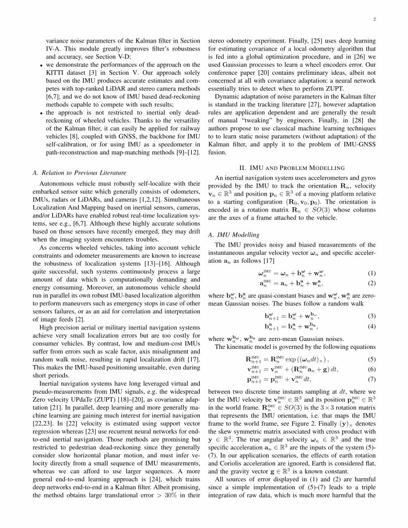
Assumptions that vlatn and vupn are roughly null are commonfor cars moving forward on human made roads or wheeledrobots moving indoor. Treating them as loose constraints, i.e.,allowing the uncertainty encoded in Nn to be non strictly null,leads to much better estimates than treating them as strictlynull [13].

It should be duly noted the vertical velocity vupn is expressedin the car frame, and thus the assumption it is roughly nullgenerally holds for a car moving on a road even if the motionis 3D. It is quite different from assuming null vertical velocityin the world frame, which then boils down to planar horizontalmotion.

The main point of the present work is that the validity ofthe null lateral and vertical velocity assumptions widely varydepending on what maneuver is being performed: for instance,vlatn is much larger in turns than in straight lines. The roleof the noise parameter adapter of Section IV-A, based on AItechniques, will be to dynamically assess the parameter Nn

that reflects confidence in the assumptions, as a function ofpast and present IMU measurements.

C. The Invariant Extended Kalman Filter (IEKF)

PropagationωIMUn

aIMUn

Nn+1

Update xn+1,Pn+1

Invariant Extended Kalman Filter

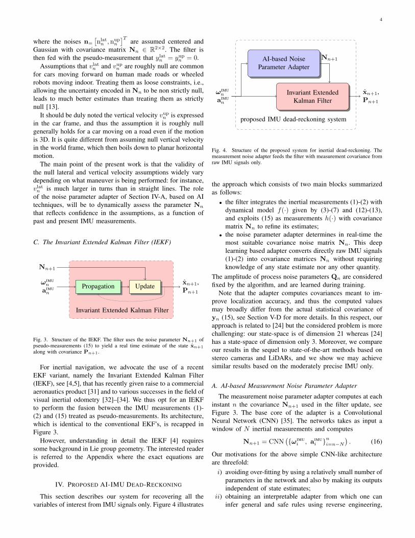
Fig. 3. Structure of the IEKF. The filter uses the noise parameter Nn+1 ofpseudo-measurements (15) to yield a real time estimate of the state xn+1

along with covariance Pn+1.

For inertial navigation, we advocate the use of a recentEKF variant, namely the Invariant Extended Kalman Filter(IEKF), see [4,5], that has recently given raise to a commercialaeronautics product [31] and to various successes in the field ofvisual inertial odometry [32]–[34]. We thus opt for an IEKFto perform the fusion between the IMU measurements (1)-(2) and (15) treated as pseudo-measurements. Its architecture,which is identical to the conventional EKF’s, is recapped inFigure 3.

However, understanding in detail the IEKF [4] requiressome background in Lie group geometry. The interested readeris referred to the Appendix where the exact equations areprovided.

IV. PROPOSED AI-IMU DEAD-RECKONING

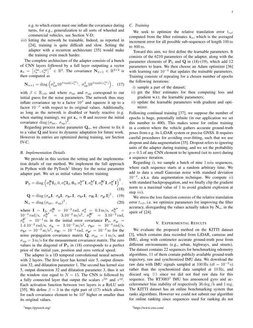
This section describes our system for recovering all thevariables of interest from IMU signals only. Figure 4 illustrates

Invariant ExtendedKalman Filter

ωIMUn

aIMUn

xn+1,Pn+1

AI-based NoiseParameter Adapter

proposed IMU dead-reckoning system

Nn+1

Fig. 4. Structure of the proposed system for inertial dead-reckoning. Themeasurement noise adapter feeds the filter with measurement covariance fromraw IMU signals only.

the approach which consists of two main blocks summarizedas follows:• the filter integrates the inertial measurements (1)-(2) with

dynamical model f(·) given by (3)-(7) and (12)-(13),and exploits (15) as measurements h(·) with covariancematrix Nn to refine its estimates;

• the noise parameter adapter determines in real-time themost suitable covariance noise matrix Nn. This deeplearning based adapter converts directly raw IMU signals(1)-(2) into covariance matrices Nn without requiringknowledge of any state estimate nor any other quantity.

The amplitude of process noise parameters Qn are consideredfixed by the algorithm, and are learned during training.

Note that the adapter computes covariances meant to im-prove localization accuracy, and thus the computed valuesmay broadly differ from the actual statistical covariance ofyn (15), see Section V-D for more details. In this respect, ourapproach is related to [24] but the considered problem is morechallenging: our state-space is of dimension 21 whereas [24]has a state-space of dimension only 3. Moreover, we compareour results in the sequel to state-of-the-art methods based onstereo cameras and LiDARs, and we show we may achievesimilar results based on the moderately precise IMU only.

A. AI-based Measurement Noise Parameter Adapter

The measurement noise parameter adapter computes at eachinstant n the covariance Nn+1 used in the filter update, seeFigure 3. The base core of the adapter is a ConvolutionalNeural Network (CNN) [35]. The networks takes as input awindow of N inertial measurements and computes

Nn+1 = CNN({ωIMU

i , aIMUi }

ni=n−N

). (16)

Our motivations for the above simple CNN-like architectureare threefold:i) avoiding over-fitting by using a relatively small number of

parameters in the network and also by making its outputsindependent of state estimates;

ii) obtaining an interpretable adapter from which one caninfer general and safe rules using reverse engineering,

5

e.g. to which extent must one inflate the covariance duringturns, for e.g., generalization to all sorts of wheeled andcommercial vehicles, see Section V-D;

iii) letting the network be trainable. Indeed, as reported in[24], training is quite difficult and slow. Setting theadapter with a recurrent architecture [35] would makethe training even much harder.

The complete architecture of the adapter consists of a bunchof CNN layers followed by a full layer outputting a vectorzn =

[zlatn , zupn

]T ∈ R2. The covariance Nn+1 ∈ R2×2 isthen computed as

Nn+1 = diag(σ2lat10

β tanh(zlatn ), σ2up10

β tanh(zupn )), (17)

with β ∈ R>0, and where σlat and σup correspond to ourinitial guess for the noise parameters. The network thus mayinflate covariance up to a factor 10β and squeeze it up to afactor 10−β with respect to its original values. Additionally,as long as the network is disabled or barely reactive (e.g.when starting training), we get zn ≈ 0 and recover the initialcovariance diag (σlat, σup)

2.Regarding process noise parameter Qn, we choose to fix it

to a value Q and leave its dynamic adaptation for future work.However its entries are optimized during training, see SectionIV-C.

B. Implementation Details

We provide in this section the setting and the implementa-tion details of our method. We implement the full approachin Python with the PyTorch1 library for the noise parameteradapter part. We set as initial values before training

P0 = diag(σR0 I2, 0, σ

v0 I2,04, σ

bω

0 I, σba

0 I, σRc

0 I, σpc

0 I)2,

(18)

Q = diag (σωI, σaI, σbωI, σbaI, σRcI, σpcI)2, (19)

Nn = diag (σlat, σup)2, (20)

where I = I3, σR0 = 10−3 rad, σv

0 = 0.3m/s, σbω

0 =10−4 rad/s, σba

0 = 3.10−2 m/s2, σRc

0 = 3.10−3 rad,σpc

0 = 10−1 m in the initial error covariance P0, σω =1.4.10−2 rad/s, σa = 3.10−2 m/s2, σbω = 10−4 rad/s,σba = 10−3 m/s2, σRc = 10−4 rad, σpc = 10−4 m for thenoise propagation covariance matrix Q, σlat = 1m/s, andσup = 3m/s for the measurement covariance matrix. The zerovalues in the diagonal of P0 in (18) corresponds to a perfectprior of the initial yaw, position and zero vertical speed.

The adapter is a 1D temporal convolutional neural networkwith 2 layers. The first layer has kernel size 5, output dimen-sion 32, and dilatation parameter 1. The second has kernel size5, output dimension 32 and dilatation parameter 3, thus it setthe window size equal to N = 15. The CNN is followed bya fully connected layer that output the scalars zlat and zup.Each activation function between two layers is a ReLU unit[35]. We define β = 3 in the right part of (17) which allowsfor each covariance element to be 103 higher or smaller thanits original values.

1https://pytorch.org/

C. Training

We seek to optimize the relative translation error trelcomputed from the filter estimates xn, which is the averagedincrement error for all possible sub-sequences of length 100mto 800m.

Toward this aim, we first define the learnable parameters. Itconsists of the 6210 parameters of the adapter, along with theparameter elements of P0 and Q in (18)-(19), which add 12parameters to learn. We then choose an Adam optimizer [36]with learning rate 10−4 that updates the trainable parameters.Training consists of repeating for a chosen number of epochsthe following iterations:i) sample a part of the dataset;ii) get the filter estimates for then computing loss and

gradient w.r.t. the learnable parameters;ii) update the learnable parameters with gradient and opti-

mizer.Following continual training [37], we suppose the number ofepochs is huge, potentially infinite (in our application we setthis number to 400). This makes sense for online trainingin a context where the vehicle gathers accurate ground-truthposes from e.g. its LiDAR system or precise GNSS. It requirescareful procedures for avoiding over-fitting, such that we usedropout and data augmentation [35]. Dropout refers to ignoringunits of the adapter during training, and we set the probabilityp = 0.5 of any CNN element to be ignored (set to zero) duringa sequence iteration.

Regarding i), we sample a batch of nine 1min sequences,where each sequence starts at a random arbitrary time. Weadd to data a small Gaussian noise with standard deviation10−4, a.k.a. data augmentation technique. We compute ii)with standard backpropagation, and we finally clip the gradientnorm to a maximal value of 1 to avoid gradient explosion atstep iii).

We stress the loss function consists of the relative translationerror trel, i.e. we optimize parameters for improving the filteraccuracy, disregarding the values actually taken by Nn, in thespirit of [24].

V. EXPERIMENTAL RESULTS

We evaluate the proposed method on the KITTI dataset[3], which contains data recorded from LiDAR, cameras andIMU, along with centimeter accurate ground-truth pose fromdifferent environments (e.g., urban, highways, and streets).The dataset contains 22 sequences for benchmarking odometryalgorithms, 11 of them contain publicly available ground-truthtrajectory, raw and synchronized IMU data. We download theraw data with IMU signals sampled at 100Hz (dt = 10−2 s)rather than the synchronized data sampled at 10Hz, anddiscard seq. 03 since we did not find raw data for thissequence. The RT30032 IMU has announced gyro and ac-celerometer bias stability of respectively 36 deg /h and 1mg.The KITTI dataset has an online benchmarking system thatranks algorithms. However we could not submit our algorithmfor online ranking since sequences used for ranking do not

2https://www.oxts.com/

6

testseq. environment

IMLS [6] ORB-SLAM2 [7] IMU proposedlength duration trel rrel trel rrel trel rrel trel rrel(km) (s) (%) (deg/m) (%) (deg/m) (%) (deg/m) (%) (deg/m)

01 2.6 110 highway 0.48 0.08 1.38 0.20 5.35 0.12 1.11 0.1203 - 80 country - - - - - - - -04 0.4 27 country 0.25 0.08 0.41 0.21 0.97 0.10 0.35 0.0806 1.2 110 urban 0.78 0.07 0.89 0.22 5.78 0.19 0.97 0.2007 0.7 110 urban 0.32 0.12 1.16 0.49 12.6 0.30 0.84 0.3208 3.2 407 urban, country 1.84 0.17 1.52 0.30 549 0.56 1.48 0.3209 1.7 159 urban, country 0.97 0.11 1.01 0.25 23.4 0.32 0.80 0.2210 0.9 120 urban, country 0.50 0.14 0.31 0.34 4.58 0.25 0.98 0.23

average scores 0.98 0.12 1.17 0.27 171 0.31 1.10 0.23

Table 1. Results on [3]. IMU integration tends to drift or diverge, whereas the proposed method may be used as an alternative to LiDAR based (IMLS) andstereo vision based (ORB-SLAM2) methods, using only IMU information. Indeed, on average, our dead-reckoning solution performs better than ORB-SLAM2and achieves a translational error being close to that of the LiDAR based method IMLS, which is ranked 3rd on the KITTI online benchmarking system. Datafrom seq. 03 was unavailable for testing algorithms, and sequences 00, 02 and 05 are discussed separately in Section V-C. It should be duly noted IMLS,ORB-SLAM2, and the proposed AI-IMU algorithm, all use different sensors. The interest of ranking algorithms based on different information is debatable.Our goal here is rather to evidence that using data from a moderately precise IMU only, one can achieve similar results as state of the art systems based onimaging sensors, which is a rather surprising feature.

contain IMU data, which is reserved for training only. Ourimplementation is made open-source at:

https://github.com/mbrossar/ai-imu-dr.

A. Evaluation Metrics and Compared Methods

To assess performances we consider the two error metricsproposed in [3]:

1) Relative Translation Error (trel): which is the aver-aged relative translation increment error for all possible sub-sequences of length 100m, . . . , 800m, in percent of thetraveled distance;

2) Relative Rotational Error (trel): that is the relativerotational increment error for all possible sub-sequences oflength 100m, . . . , 800m, in degree per meter.

We compare four methods which alternatively use LiDAR,stereo vision, and IMU-based estimations:• IMLS [6]: a recent state-of-the-art LiDAR-based ap-

proach ranked 3rd in the KITTI benchmark. The authorprovided us with the code after disabling the loop-closuremodule;

• ORB-SLAM2 [7]: a popular and versatile library formonocular, stereo and RGB-D cameras that computesa sparse reconstruction of the map. We took the open-source code, disable loop-closure capability and evaluatethe stereo algorithm without modifying any parameter;

• IMU: the direct integration of the IMU measurementsbased on (4)-(5), that is, pure inertial navigation;

• proposed: the proposed approach, that uses only the IMUsignals and involves no other sensor.

B. Trajectory Results

We follow the same protocol for evaluating each sequence:i) we initialize the filter with parameters described in SectionIV-B; ii) we train then the noise parameter adapter followingSection IV-C for 400 epochs without the evaluated sequence

−100 −50 0 50 100 150 200

0

50

100

150

200

endstart

5 s carstop

x (m)

y(m

)ground-truth IMLS ORB-SLAM2

IMU proposed

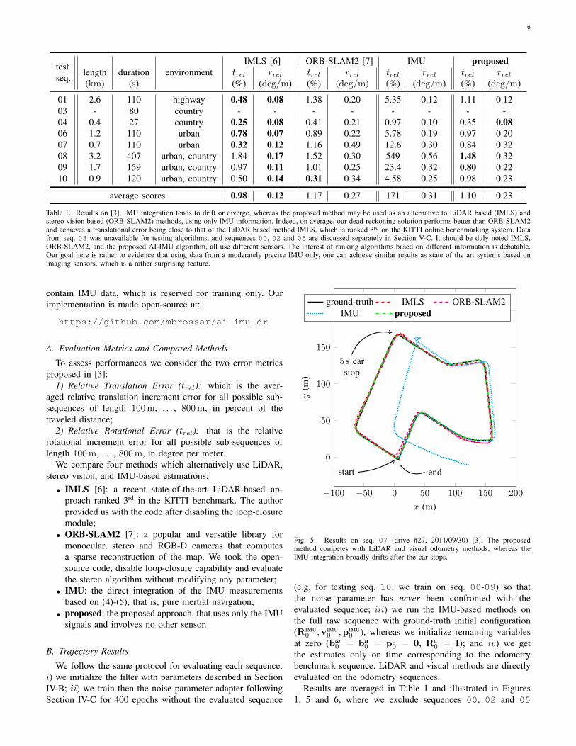
Fig. 5. Results on seq. 07 (drive #27, 2011/09/30) [3]. The proposedmethod competes with LiDAR and visual odometry methods, whereas theIMU integration broadly drifts after the car stops.

(e.g. for testing seq. 10, we train on seq. 00-09) so thatthe noise parameter has never been confronted with theevaluated sequence; iii) we run the IMU-based methods onthe full raw sequence with ground-truth initial configuration(RIMU

0 ,vIMU0 ,pIMU

0 ), whereas we initialize remaining variablesat zero (bω0 = ba

0 = pc0 = 0, Rc

0 = I); and iv) we getthe estimates only on time corresponding to the odometrybenchmark sequence. LiDAR and visual methods are directlyevaluated on the odometry sequences.

Results are averaged in Table 1 and illustrated in Figures1, 5 and 6, where we exclude sequences 00, 02 and 05

7

−100 0 100 200 300 400 500

−500

−400

−300

−200

−100

0

100

200

start/end

x (m)

y(m

)ground-truth IMLS ORB-SLAM2

IMU proposed

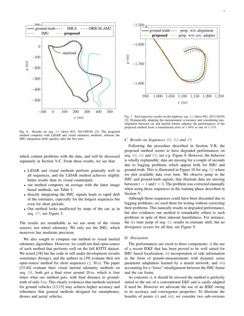
Fig. 6. Results on seq. 09 (drive #33, 2011/09/30) [3]. The proposedmethod competes with LiDAR and visual odometry methods, whereas theIMU integration drifts quickly after the first turn.

which contain problems with the data, and will be discussedseparately in Section V-C. From these results, we see that:

• LiDAR and visual methods perform generally well inall sequences, and the LiDAR method achieves slightlybetter results than its visual counterpart;

• our method competes on average with the latter imagebased methods, see Table 1;

• directly integrating the IMU signals leads to rapid driftof the estimates, especially for the longest sequences buteven for short periods;

• Our method looks unaffected by stops of the car, as inseq. 07, see Figure 5.

The results are remarkable as we use none of the visionsensors, nor wheel odometry. We only use the IMU, whichmoreover has moderate precision.

We also sought to compare our method to visual inertialodometry algorithms. However, we could not find open-sourceof such method that performs well on the full KITTI dataset.We tested [38] but the code in still under development (resultssometimes diverge), and the authors in [39] evaluate their notopen-source method for short sequences (≤ 30 s). The paper[33,40] evaluate their visual inertial odometry methods onseq. 08, both get a final error around 20m, which is fourtimes what our method gets, with final distance to ground-truth of only 5m. This clearly evidences that methods tayloredfor ground vehicles [13,15] may achieve higher accuracy androbustness that general methods designed for smartphones,drones and aerial vehicles.

950 1,000 1,050 1,100 1,150 1,200 1,250

−1,800

−1,700

−1,600

−1,500

x (m)

y(m

)

ground-truth prop. w/o alignmentproposed prop. w/o cov. adapter

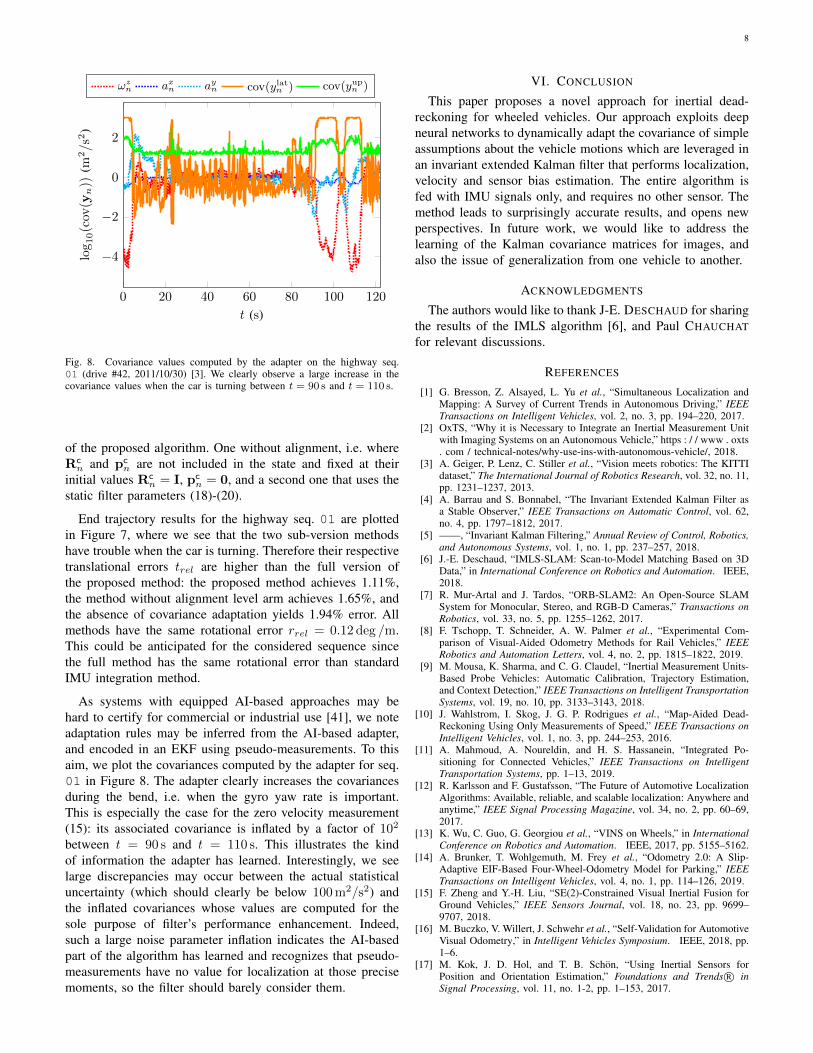
Fig. 7. End trajectory results on the highway seq. 01 (drive #42, 2011/10/30)[3]. Dynamically adapting the measurement covariance and considering mis-alignment between car and inertial frames enhance the performances of theproposed method from a translational error of 1.94% to one of 1.11%.

C. Results on Sequences 00, 02 and 05

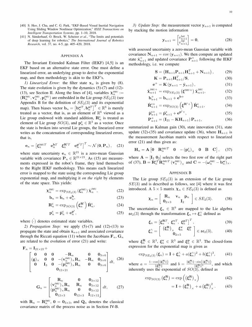
Following the procedure described in Section V-B, theproposed method seems to have degraded performances onseq. 00, 02 and 05, see e.g. Figure 9. However, the behavioris wholly explainable: data are missing for a couple of secondsdue to logging problems which appear both for IMU andground-truth. This is illustrated in Figure 10 for seq. 02 wherewe plot available data over time. We observe jump in theIMU and ground-truth signals, that illustrate data are missingbetween t = 1 and t = 3. The problem was corrected manuallywhen using those sequences in the training phase described inSection V.

Although those sequences could have been discarded due tologging problems, we used them for testing without correctingtheir problems. This naturally results in degraded performance,but also evidences our method is remarkably robust to suchproblems in spite of their inherent harmfulness. For instance,the 2 s time jump of seq. 02 results in estimate shift, but nodivergence occurs for all that, see Figure 9.

D. Discussion

The performances are owed to three components: i) the useof a recent IEKF that has been proved to be well suited forIMU based localization; ii) incorporation of side informationin the form of pseudo-measurements with dynamic noiseparameter adaptation learned by a neural network; and iii)accounting for a “loose” misalignment between the IMU frameand the car frame.

As concerns i), it should be stressed the method is perfectlysuited to the use of a conventional EKF and is easily adaptedif need be. However we advocate the use of an IEKF owingto its accuracy and convergence properties. To illustrate thebenefits of points ii) and iii), we consider two sub-versions

8

0 20 40 60 80 100 120

−4

−2

0

2

t (s)

log10(cov

(yn))

(m2/s2

)ωzn ax

n ayn cov(ylat

n ) cov(yupn )

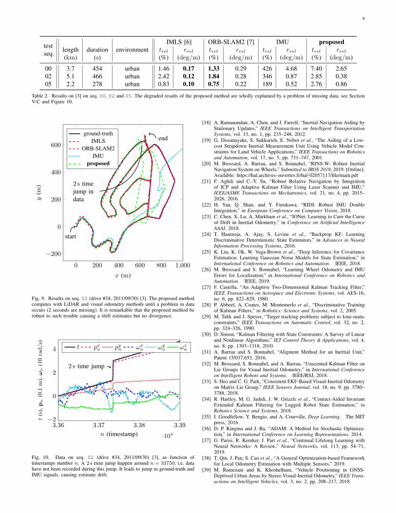
Fig. 8. Covariance values computed by the adapter on the highway seq.01 (drive #42, 2011/10/30) [3]. We clearly observe a large increase in thecovariance values when the car is turning between t = 90 s and t = 110 s.

of the proposed algorithm. One without alignment, i.e. whereRcn and pc

n are not included in the state and fixed at theirinitial values Rc

n = I, pcn = 0, and a second one that uses the

static filter parameters (18)-(20).

End trajectory results for the highway seq. 01 are plottedin Figure 7, where we see that the two sub-version methodshave trouble when the car is turning. Therefore their respectivetranslational errors trel are higher than the full version ofthe proposed method: the proposed method achieves 1.11%,the method without alignment level arm achieves 1.65%, andthe absence of covariance adaptation yields 1.94% error. Allmethods have the same rotational error rrel = 0.12 deg /m.This could be anticipated for the considered sequence sincethe full method has the same rotational error than standardIMU integration method.

As systems with equipped AI-based approaches may behard to certify for commercial or industrial use [41], we noteadaptation rules may be inferred from the AI-based adapter,and encoded in an EKF using pseudo-measurements. To thisaim, we plot the covariances computed by the adapter for seq.01 in Figure 8. The adapter clearly increases the covariancesduring the bend, i.e. when the gyro yaw rate is important.This is especially the case for the zero velocity measurement(15): its associated covariance is inflated by a factor of 102

between t = 90 s and t = 110 s. This illustrates the kindof information the adapter has learned. Interestingly, we seelarge discrepancies may occur between the actual statisticaluncertainty (which should clearly be below 100m2/s2) andthe inflated covariances whose values are computed for thesole purpose of filter’s performance enhancement. Indeed,such a large noise parameter inflation indicates the AI-basedpart of the algorithm has learned and recognizes that pseudo-measurements have no value for localization at those precisemoments, so the filter should barely consider them.

VI. CONCLUSION

This paper proposes a novel approach for inertial dead-reckoning for wheeled vehicles. Our approach exploits deepneural networks to dynamically adapt the covariance of simpleassumptions about the vehicle motions which are leveraged inan invariant extended Kalman filter that performs localization,velocity and sensor bias estimation. The entire algorithm isfed with IMU signals only, and requires no other sensor. Themethod leads to surprisingly accurate results, and opens newperspectives. In future work, we would like to address thelearning of the Kalman covariance matrices for images, andalso the issue of generalization from one vehicle to another.

ACKNOWLEDGMENTS

The authors would like to thank J-E. DESCHAUD for sharingthe results of the IMLS algorithm [6], and Paul CHAUCHATfor relevant discussions.

REFERENCES

[1] G. Bresson, Z. Alsayed, L. Yu et al., “Simultaneous Localization andMapping: A Survey of Current Trends in Autonomous Driving,” IEEETransactions on Intelligent Vehicles, vol. 2, no. 3, pp. 194–220, 2017.

[2] OxTS, “Why it is Necessary to Integrate an Inertial Measurement Unitwith Imaging Systems on an Autonomous Vehicle,” https : / / www . oxts. com / technical-notes/why-use-ins-with-autonomous-vehicle/, 2018.

[3] A. Geiger, P. Lenz, C. Stiller et al., “Vision meets robotics: The KITTIdataset,” The International Journal of Robotics Research, vol. 32, no. 11,pp. 1231–1237, 2013.

[4] A. Barrau and S. Bonnabel, “The Invariant Extended Kalman Filter asa Stable Observer,” IEEE Transactions on Automatic Control, vol. 62,no. 4, pp. 1797–1812, 2017.

[5] ——, “Invariant Kalman Filtering,” Annual Review of Control, Robotics,and Autonomous Systems, vol. 1, no. 1, pp. 237–257, 2018.

[6] J.-E. Deschaud, “IMLS-SLAM: Scan-to-Model Matching Based on 3DData,” in International Conference on Robotics and Automation. IEEE,2018.

[7] R. Mur-Artal and J. Tardos, “ORB-SLAM2: An Open-Source SLAMSystem for Monocular, Stereo, and RGB-D Cameras,” Transactions onRobotics, vol. 33, no. 5, pp. 1255–1262, 2017.

[8] F. Tschopp, T. Schneider, A. W. Palmer et al., “Experimental Com-parison of Visual-Aided Odometry Methods for Rail Vehicles,” IEEERobotics and Automation Letters, vol. 4, no. 2, pp. 1815–1822, 2019.

[9] M. Mousa, K. Sharma, and C. G. Claudel, “Inertial Measurement Units-Based Probe Vehicles: Automatic Calibration, Trajectory Estimation,and Context Detection,” IEEE Transactions on Intelligent TransportationSystems, vol. 19, no. 10, pp. 3133–3143, 2018.

[10] J. Wahlstrom, I. Skog, J. G. P. Rodrigues et al., “Map-Aided Dead-Reckoning Using Only Measurements of Speed,” IEEE Transactions onIntelligent Vehicles, vol. 1, no. 3, pp. 244–253, 2016.

[11] A. Mahmoud, A. Noureldin, and H. S. Hassanein, “Integrated Po-sitioning for Connected Vehicles,” IEEE Transactions on IntelligentTransportation Systems, pp. 1–13, 2019.

[12] R. Karlsson and F. Gustafsson, “The Future of Automotive LocalizationAlgorithms: Available, reliable, and scalable localization: Anywhere andanytime,” IEEE Signal Processing Magazine, vol. 34, no. 2, pp. 60–69,2017.

[13] K. Wu, C. Guo, G. Georgiou et al., “VINS on Wheels,” in InternationalConference on Robotics and Automation. IEEE, 2017, pp. 5155–5162.

[14] A. Brunker, T. Wohlgemuth, M. Frey et al., “Odometry 2.0: A Slip-Adaptive EIF-Based Four-Wheel-Odometry Model for Parking,” IEEETransactions on Intelligent Vehicles, vol. 4, no. 1, pp. 114–126, 2019.

[15] F. Zheng and Y.-H. Liu, “SE(2)-Constrained Visual Inertial Fusion forGround Vehicles,” IEEE Sensors Journal, vol. 18, no. 23, pp. 9699–9707, 2018.

[16] M. Buczko, V. Willert, J. Schwehr et al., “Self-Validation for AutomotiveVisual Odometry,” in Intelligent Vehicles Symposium. IEEE, 2018, pp.1–6.

[17] M. Kok, J. D. Hol, and T. B. Schon, “Using Inertial Sensors forPosition and Orientation Estimation,” Foundations and Trends R© inSignal Processing, vol. 11, no. 1-2, pp. 1–153, 2017.

9

testseq. environment

IMLS [6] ORB-SLAM2 [7] IMU proposedlength duration trel rrel trel rrel trel rrel trel rrel(km) (s) (%) (deg/m) (%) (deg/m) (%) (deg/m) (%) (deg/m)

00 3.7 454 urban 1.46 0.17 1.33 0.29 426 4.68 7.40 2.6502 5.1 466 urban 2.42 0.12 1.84 0.28 346 0.87 2.85 0.3805 2.2 278 urban 0.83 0.10 0.75 0.22 189 0.52 2.76 0.86

Table 2. Results on [3] on seq. 00, 02 and 05. The degraded results of the proposed method are wholly explained by a problem of missing data, see SectionV-C and Figure 10.

0 200 400 600 800 1,000

−200

0

200

400

600

start

2 s timejump indata

end

x (m)

y(m

)

ground-truthIMLS

ORB-SLAM2IMU

proposed

Fig. 9. Results on seq. 02 (drive #34, 2011/09/30) [3]. The proposed methodcompetes with LiDAR and visual odometry methods until a problem in dataoccurs (2 seconds are missing). It is remarkable that the proposed method berobust to such trouble causing a shift estimates but no divergence.

3.36 3.37 3.38 3.39

·104

−2

0

2

4

2 s time jump

n (timestamp)

t(s

),pn

(0.1

m),ω

n(1

0rad/s)

t pxn pyn ωxn ωy

n ωzn

Fig. 10. Data on seq. 02 (drive #34, 2011/09/30) [3], as function oftimestamps number n. A 2 s time jump happen around n = 33750, i.e. datahave not been recorded during this jump. It leads to jump in ground-truth andIMU signals, causing estimate drift.

[18] A. Ramanandan, A. Chen, and J. Farrell, “Inertial Navigation Aiding byStationary Updates,” IEEE Transactions on Intelligent TransportationSystems, vol. 13, no. 1, pp. 235–248, 2012.

[19] G. Dissanayake, S. Sukkarieh, E. Nebot et al., “The Aiding of a Low-cost Strapdown Inertial Measurement Unit Using Vehicle Model Con-straints for Land Vehicle Applications,” IEEE Transactions on Roboticsand Automation, vol. 17, no. 5, pp. 731–747, 2001.

[20] M. Brossard, A. Barrau, and S. Bonnabel, “RINS-W: Robust InertialNavigation System on Wheels,” Submitted to IROS 2019, 2019. [Online].Available: https://hal.archives-ouvertes.fr/hal-02057117/file/main.pdf

[21] F. Aghili and C.-Y. Su, “Robust Relative Navigation by Integrationof ICP and Adaptive Kalman Filter Using Laser Scanner and IMU,”IEEE/ASME Transactions on Mechatronics, vol. 21, no. 4, pp. 2015–2026, 2016.

[22] H. Yan, Q. Shan, and Y. Furukawa, “RIDI: Robust IMU DoubleIntegration,” in European Conference on Computer Vision, 2018.

[23] C. Chen, X. Lu, A. Markham et al., “IONet: Learning to Cure the Curseof Drift in Inertial Odometry,” in Conference on Artificial IntelligenceAAAI, 2018.

[24] T. Haarnoja, A. Ajay, S. Levine et al., “Backprop KF: LearningDiscriminative Deterministic State Estimators,” in Advances in NeuralInformation Processing Systems, 2016.

[25] K. Liu, K. Ok, W. Vega-Brown et al., “Deep Inference for CovarianceEstimation: Learning Gaussian Noise Models for State Estimation,” inInternational Conference on Robotics and Automation. IEEE, 2018.

[26] M. Brossard and S. Bonnabel, “Learning Wheel Odometry and IMUErrors for Localization,” in International Conference on Robotics andAutomation. IEEE, 2019.

[27] F. Castella, “An Adaptive Two-Dimensional Kalman Tracking Filter,”IEEE Transactions on Aerospace and Electronic Systems, vol. AES-16,no. 6, pp. 822–829, 1980.

[28] P. Abbeel, A. Coates, M. Montemerlo et al., “Discriminative Trainingof Kalman Filters,” in Robotics: Science and Systems, vol. 2, 2005.

[29] M. Tahk and J. Speyer, “Target tracking problems subject to kine-maticconstraints,” IEEE Transactions on Automatic Control, vol. 32, no. 2,pp. 324–326, 1990.

[30] D. Simon, “Kalman Filtering with State Constraints: A Survey of Linearand Nonlinear Algorithms,” IET Control Theory & Applications, vol. 4,no. 8, pp. 1303–1318, 2010.

[31] A. Barrau and S. Bonnabel, “Aligment Method for an Inertial Unit,”Patent 15/037,653, 2016.

[32] M. Brossard, S. Bonnabel, and A. Barrau, “Unscented Kalman Filter onLie Groups for Visual Inertial Odometry,” in International Conferenceon Intelligent Robots and Systems. IEEE/RSJ, 2018.

[33] S. Heo and C. G. Park, “Consistent EKF-Based Visual-Inertial Odometryon Matrix Lie Group,” IEEE Sensors Journal, vol. 18, no. 9, pp. 3780–3788, 2018.

[34] R. Hartley, M. G. Jadidi, J. W. Grizzle et al., “Contact-Aided InvariantExtended Kalman Filtering for Legged Robot State Estimation,” inRobotics Science and Systems, 2018.

[35] I. Goodfellow, Y. Bengio, and A. Courville, Deep Learning. The MITpress, 2016.

[36] D. P. Kingma and J. Ba, “ADAM: A Method for Stochastic Optimiza-tion,” in International Conference on Learning Representations, 2014.

[37] G. Parisi, R. Kemker, J. Part et al., “Continual Lifelong Learning withNeural Networks: A Review,” Neural Networks, vol. 113, pp. 54–71,2019.

[38] T. Qin, J. Pan, S. Cao et al., “A General Optimization-based Frameworkfor Local Odometry Estimation with Multiple Sensors,” 2019.

[39] M. Ramezani and K. Khoshelham, “Vehicle Positioning in GNSS-Deprived Urban Areas by Stereo Visual-Inertial Odometry,” IEEE Trans-actions on Intelligent Vehicles, vol. 3, no. 2, pp. 208–217, 2018.

10

[40] S. Heo, J. Cha, and C. G. Park, “EKF-Based Visual Inertial NavigationUsing Sliding Window Nonlinear Optimization,” IEEE Transactions onIntelligent Transportation Systems, pp. 1–10, 2018.

[41] N. Sunderhauf, O. Brock, W. Scheirer et al., “The limits and potentialsof deep learning for robotics,” The International Journal of RoboticsResearch, vol. 37, no. 4-5, pp. 405–420, 2018.

APPENDIX A

The Invariant Extended Kalman Filter (IEKF) [4,5] is anEKF based on an alternative state error. One must define alinearized error, an underlying group to derive the exponentialmap, and then methodology is akin to the EKF’s.

1) Linearized Error: the filter state xn is given by (8).The state evolution is given by the dynamics (5)-(7) and (12)-(13), see Section II. Along the lines of [4], variables χIMU

n :=(RIMU

n ,vIMUn ,pIMU

n ) are embedded in the Lie group SE2(3) (seeAppendix B for the definition of SE2(3) and its exponentialmap). Then biases vector bn =

[bωTn ,baT

n

]T ∈ R6 is merelytreated as a vector, that is, as an element of R6 viewed as aLie group endowed with standard addition, Rc

n is treated aselement of Lie group SO(3), and pc

n ∈ R3 as a vector. Oncethe state is broken into several Lie groups, the linearized errorwrites as the concatenation of corresponding linearized errors,that is,

en =[ξIMUTn ebTn ξR

cTn ep

cTn

]T ∼ N (0,Pn) , (21)

where state uncertainty en ∈ R21 is a zero-mean Gaussianvariable with covariance Pn ∈ R21×21. As (15) are measure-ments expressed in the robot’s frame, they lend themselvesto the Right IEKF methodology. This means each linearizederror is mapped to the state using the corresponding Lie groupexponential map, and multiplying it on the right by elementsof the state space. This yields:

χIMUn = expSE2(3) (ξ

IMUn ) χ

IMUn , (22)

bn = bn + ebn, (23)

Rcn = expSO(3)

(ξR

c

n

)Rcn, (24)

pcn = pc

n + epc

n , (25)

where (·) denotes estimated state variables.2) Propagation Step: we apply (5)-(7) and (12)-(13) to

propagate the state and obtain xn+1 and associated covariancethrough the Riccati equation (11) where the Jacobians Fn, Gn

are related to the evolution of error (21) and write:

Fn = I21×21+0 0 0 −Rn 0 03×6

(g)× 0 0 −(vIMUn )×Rn −Rn 03×6

0 I3 0 −(pIMUn )×Rn 0 03×6

012×21

dt, (26)

Gn =

Rn 0 03×12

(vIMUn )×Rn Rn 03×12

(pIMUn )×Rn 0 03×12012×3 012×3 I12×12

dt, (27)

with Rn = RIMUn , 0 = 03×3, and Qn denotes the classical

covariance matrix of the process noise as in Section IV-B.

3) Update Step: the measurement vector yn+1 is computedby stacking the motion information

yn+1 =

[vlatn+1

vupn+1

]= 0, (28)

with assessed uncertainty a zero-mean Gaussian variable withcovariance Nn+1 = cov (yn+1). We then compute an updatedstate x+

n+1 and updated covariance P+n+1 following the IEKF

methodology, i.e. we compute

S =(Hn+1Pn+1H

Tn+1 +Nn+1

), (29)

K = Pn+1HTn+1/S, (30)

e+ = K (yn+1 − yn+1) , (31)

χIMU+n+1 = expSE2(3)

(ξIMU+

)χIMUn+1, (32)

b+n+1 = bn+1 + eb+ (33)

Rc+n+1 = expSO(3)

(ξR

c+)Rcn+1, (34)

pc+n+1 = pc

n+1 + epc+, (35)

P+n+1 = (I21 −KHn+1)Pn+1, (36)

summarized as Kalman gain (30), state innovation (31), stateupdate (32)-(35) and covariance update (36), where Hn+1 isthe measurement Jacobian matrix with respect to linearizederror (21) and thus given as:

Hn = A[0 RIMUT

n 0 − (pcn)× 0 B C

], (37)

where A = [I2 02] selects the two first row of the right partof (37), B = RcT

n RIMUTn (vIMU

n )× and C = −(ωIMUn − bωn )×.

APPENDIX B

The Lie group SE2(3) is an extension of the Lie groupSE(3) and is described as follows, see [4] where it was firstintroduced. A 5× 5 matrix χn ∈ SE2(3) is defined as

χn =

[Rn vn pn02×3 I2

]∈ SE2(3). (38)

The uncertainties ξn ∈ R9 are mapped to the Lie algebrase2(3) through the transformation ξn 7→ ξ∧n defined as

ξn =[ξRTn , ξvTn , ξpTn

]T, (39)

ξ∧n =

[ (ξRn)× ξvn ξpn02×5

]∈ se2(3), (40)

where ξRn ∈ R3, ξvn ∈ R3 and ξpn ∈ R3. The closed-formexpression for the exponential map is given as

expSE2(3) (ξn) = I+ ξ∧n + a(ξ∧n )2 + b(ξ∧n )

3, (41)

where a =1−cos(‖ξRn ‖)‖ξRn ‖

and b =‖ξRn ‖−sin(‖ξ

Rn ‖)

‖ξRn ‖3, and which

inherently uses the exponential of SO(3), defined as

expSO(3)

(ξRn)= exp

((ξRn)×

)(42)

= I+(ξRn)× + a

(ξRn)2× . (43)