Aircraft Wake Vortex Measurements at Denver International ... · wake acoustics test at the Denver International Airport. The central instrument of the test was a large microphone

American Institute of Aeronautics and Astronautics

1

Aircraft Wake Vortex Measurements at Denver International Airport

Robert P. Dougherty*

OptiNav, Inc., Bellevue, WA, 98004

Frank Y. Wang †

John A. Volpe National Transportation Systems Center, Cambridge, MA, 02142

Earl R. Booth‡ and Michael E. Watts § NASA Langley Research Center, Hampton, VA, 23681

Neil Fenichel ** Microstar Laboratories, Inc., Bellevue, WA, 98004

and

Robert E. D’Errico†† Titan Corporation, Billerica, MA, 01821

Airport capacity is constrained, in part, by spacing requirements associated with the wake vortex hazard. NASA’s Wake Vortex Avoidance Project has a goal to establish the feasibility of reducing this spacing while maintaining safety. Passive acoustic phased array sensors, if shown to have operational potential, may aid in this effort by detecting and tracking the vortices. During August/September 2003, NASA and the USDOT sponsored a wake acoustics test at the Denver International Airport. The central instrument of the test was a large microphone phased array. This paper describes the test in general terms and gives an overview of the array hardware. It outlines one of the analysis techniques that is being applied to the data and gives sample results. The technique is able to clearly resolve the wake vortices of landing aircraft and measure their separation, height, and sinking rate. These observations permit an indirect estimate of the vortex circulation. The array also provides visualization of the vortex evolution, including the Crow instability.

Nomenclature

iα = weight factor for microphone i in array shading

Γ = circulation ρ = density of air

b = transverse separation of vortices. The initial value after roll up is 0b .

B = beamforming sum L = lift N = number of microphones in the array

* President, 10914 NE 18 ST, Senior Member AIAA † Aerospace Engineer, Surveillance and Assessment Division, DTS-53, Senior Member AIAA ‡ Senior Research Engineer, Aeroacoustics Branch, MS 461 § Rotorcraft Section Deputy Manager, MS 254, Associate Fellow ** President, 2265 116th Avenue †† Program Manager, Volpe Center, CNS III, 700 Technology Park Drive

https://ntrs.nasa.gov/search.jsp?R=20040070828 2020-03-24T22:45:07+00:00Z


2

( )tpi = acoustic pressure measured at microphone i at time t, after filtering and decimation

r = radius of a microphone location from the center of the array. Used for array shading. s = wing span U = free-stream velocity

0V = initial vortex sink rate

I. Introduction

NE of the limiting factors restricting aircraft landings at major airports is the minimum spacing requirements due to vortex wake avoidance. If it can be shown that the separation requirements are too conservative, then it

may be possible to increase the rate of landings on a given runway. For example, if the in-trail separation requirements can be reduced by 25%, then a theoretical 33% increase in landings is possible. A thirty-three percent increase likely represents an upper limit, however, as that reduced spacing is approximately equivalent to the amount of time required for an aircraft to exit the runway after landing. Still, a 33% increase in landings makes three runways with reduced aircraft spacing equivalent to four runways without the separation reduction.

In order to investigate the possibility of safely reducing aircraft spacing, the NASA Airspace Systems Program has undertaken the Wake Vortex Avoidance Project. Its goal is to investigate the use of short term, near-real-time weather and vortex dissipation predictions and on-line verification sensors to allow airport traffic controllers to dynamically reduce aircraft spacing as conditions warrant. The system would increase airport capacity while maintaining safety by more accurately tracking wake vortex conditions.

Most of the sensors proposed for tracking wake vortices are LIDAR systems, which can not only track vortex trajectory, but can also estimate vortex strength. Passive acoustic phased array sensors have also been suggested as a mean of detecting, tracking and quantifying the vortices. If they can be shown to have operational potential, they may contribute to this effort to safely reduce spacing. A system that has been used is the microphone phased array employed in Ref. 1. Another such system is SOCRATES - Sensor for Optically Characterizing Ring-eddy Atmospheric Turbulence Emanating Sound under development by Flight Safety Technologies and Lockheed-Martin that employs a laser-based acoustic technique.2

NASA, in cooperation with Volpe National Transportation Center, through Titan, financed OptiNav and Microstar to design, build, and operate a large microphone array at the Denver airport in August/September 2003 for the purpose of capturing vortex wake acoustic signatures. The acoustic data were supplemented by a wide array of additional sensors, including two types of LIDAR, sodar, meteorological instrumentation, SOCRATES, and two DLR microphone arrays. The objectives of the test were to obtain a benchmark set of wake acoustic data supplemented by other sensors for fundamental analysis, assess improvements in the SOCRATES instrumentation, and benchmark the new acoustic array with the DLR array. This report will document the test arrangement, location and type of each sensor deployed, as well as present preliminary acoustic results obtained with the NASA/Volpe array.

II. Trailing Vortices Some elementary properties of trailing vortices are mentioned below. The reviews in Refs. 3-6 should be

consulted for more details.

A. Strength and Separation of the Initial Vortices According to the Kutta-Joukowski theorem,7 the lift per unit length of a wing can be expressed

as UdydL Γ= ρ/ , where Γ is the circulation of the bound vortex running along the trailing edge of the wing. In the

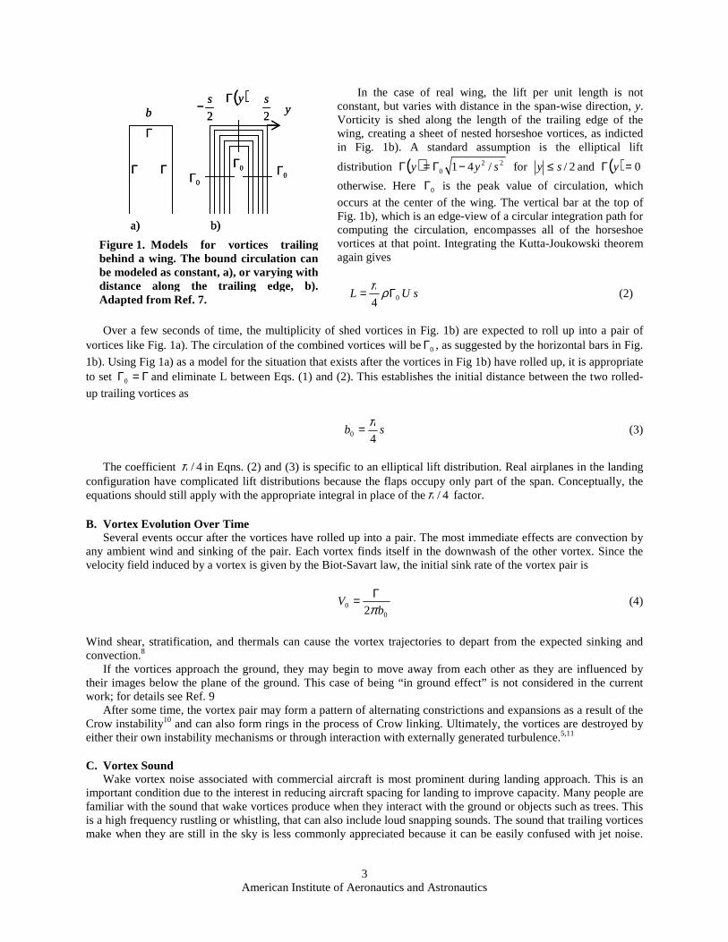
simplest case, Γ is uniform. A continuous vortex filament, as required by Helmholtz’s theorem, is completed by a pair of counter-rotating wingtip vortices trailing aft. The circulation has the same value, Γ , on each of the three segments of the horseshoe vortex, as indicated in Fig. 1a). In this case, the separation between the trailing vortices, b, is equal to the wing span, s. The total lift of the wing is obtained by integrating the Kutta-Joukowski theorem:

bUL Γ= ρ (1)

O


3

In the case of real wing, the lift per unit length is not constant, but varies with distance in the span-wise direction, y.Vorticity is shed along the length of the trailing edge of the wing, creating a sheet of nested horseshoe vortices, as indicted in Fig. 1b). A standard assumption is the elliptical lift

distribution ( ) 220 /41 syy −Γ=Γ for 2/sy ≤ and ( ) 0=Γ y

otherwise. Here 0Γ is the peak value of circulation, which

occurs at the center of the wing. The vertical bar at the top of Fig. 1b), which is an edge-view of a circular integration path for computing the circulation, encompasses all of the horseshoe vortices at that point. Integrating the Kutta-Joukowski theorem again gives

sUL 04Γ= ρπ

(2)

Over a few seconds of time, the multiplicity of shed vortices in Fig. 1b) are expected to roll up into a pair of vortices like Fig. 1a). The circulation of the combined vortices will be 0Γ , as suggested by the horizontal bars in Fig.

1b). Using Fig 1a) as a model for the situation that exists after the vortices in Fig 1b) have rolled up, it is appropriate to set Γ=Γ0 and eliminate L between Eqs. (1) and (2). This establishes the initial distance between the two rolled-

up trailing vortices as

sb40

π= (3)

The coefficient 4/π in Eqns. (2) and (3) is specific to an elliptical lift distribution. Real airplanes in the landing configuration have complicated lift distributions because the flaps occupy only part of the span. Conceptually, the equations should still apply with the appropriate integral in place of the 4/π factor.

B. Vortex Evolution Over Time Several events occur after the vortices have rolled up into a pair. The most immediate effects are convection by

any ambient wind and sinking of the pair. Each vortex finds itself in the downwash of the other vortex. Since the velocity field induced by a vortex is given by the Biot-Savart law, the initial sink rate of the vortex pair is

0

0 2 bV

πΓ= (4)

Wind shear, stratification, and thermals can cause the vortex trajectories to depart from the expected sinking and convection.8

If the vortices approach the ground, they may begin to move away from each other as they are influenced by their images below the plane of the ground. This case of being “in ground effect” is not considered in the current work; for details see Ref. 9

After some time, the vortex pair may form a pattern of alternating constrictions and expansions as a result of the Crow instability10 and can also form rings in the process of Crow linking. Ultimately, the vortices are destroyed by either their own instability mechanisms or through interaction with externally generated turbulence.5,11

C. Vortex Sound Wake vortex noise associated with commercial aircraft is most prominent during landing approach. This is an

important condition due to the interest in reducing aircraft spacing for landing to improve capacity. Many people are familiar with the sound that wake vortices produce when they interact with the ground or objects such as trees. This is a high frequency rustling or whistling, that can also include loud snapping sounds. The sound that trailing vortices make when they are still in the sky is less commonly appreciated because it can be easily confused with jet noise.

Γ

ΓΓ

( )yΓ

0Γ0Γ 0Γ

y2

s

2

s−b

a) b)

Γ

ΓΓ

( )yΓ

0Γ0Γ 0Γ

y2

s

2

s−b

a) b)

Figure 1. Models for vortices trailing behind a wing. The bound circulation can be modeled as constant, a), or varying with distance along the trailing edge, b). Adapted from Ref. 7.


4

Out-of-ground-effect (OGE; defined as altitude greater than 2/0b ) wake vortex noise is a hollow, low-frequency,

howling sound that begins shortly after an airplane on approach passes overhead, and continues for a minute or so. Vortex noise is more persistent than any sound made directly by the airplane during the approach condition. Its occurrence varies with weather and airplane model.

Commercial aircraft presumably also generate wake noise during the takeoff condition, but it is difficult to hear or measure the vortex sound in this case due to interference by the jet noise.

Theories for wake vortex noise are not fully developed. Some formulations are similar to jet noise theory: turbulence is viewed as the cause of the Lighthill stress tensor.12 Other hypothesized mechanisms are unique to the vortex problem. For example, the Kirchhoff vortex is unsteady flow associated with the rotation of an elliptical core.1,13

III. Test Setup In order to characterize the acoustic signature of wake vortices in the OGE regime, measurements were

conducted at a location under the flight path of runway 16L at the Denver International Airport. The test site is two nautical miles from the runway threshold where the nominal arriving aircraft altitude is approximately 700 feet. The selection of DIA was motivated both by its diverse aircraft mix and the relatively pristine acoustic environment. Ninety nine percent of the microphone measurements were made under Visual Meteorological Conditions (VMC).

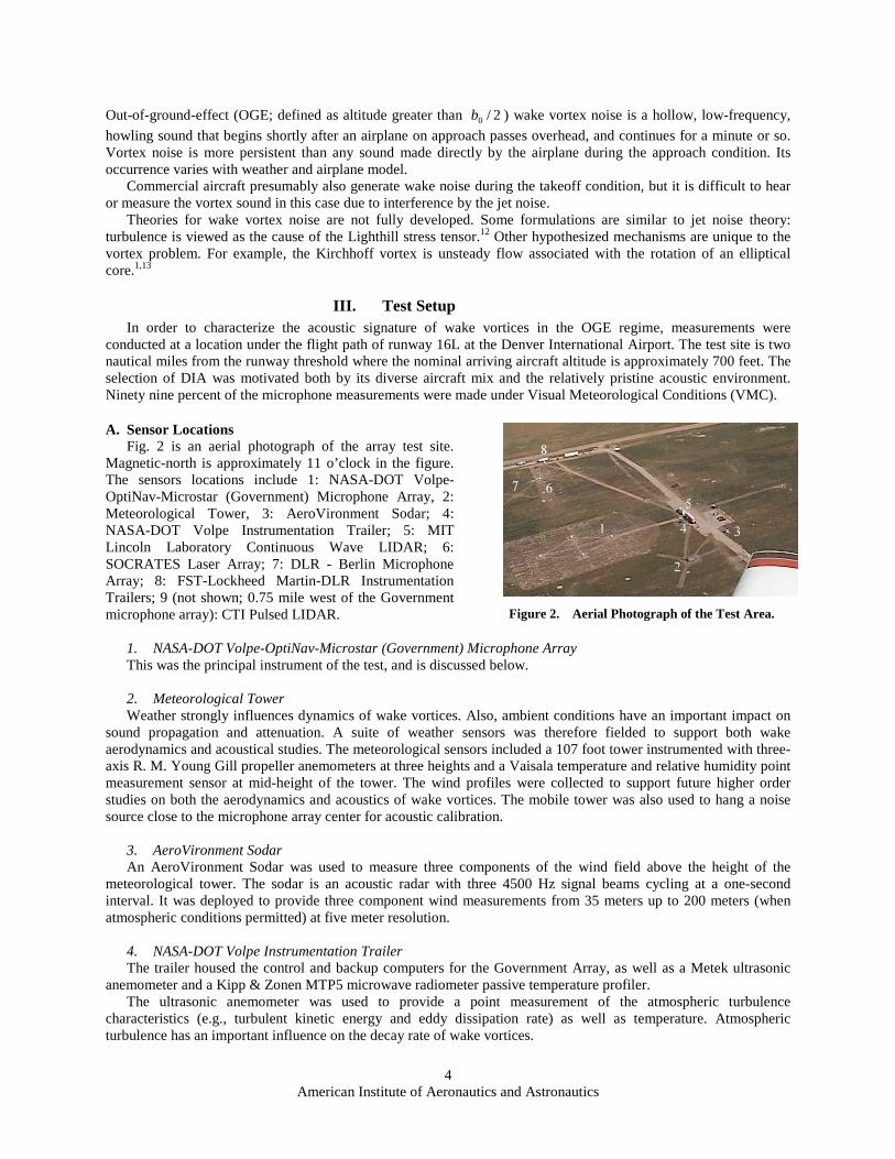
A. Sensor Locations Fig. 2 is an aerial photograph of the array test site.

Magnetic-north is approximately 11 o’clock in the figure. The sensors locations include 1: NASA-DOT Volpe-OptiNav-Microstar (Government) Microphone Array, 2: Meteorological Tower, 3: AeroVironment Sodar; 4: NASA-DOT Volpe Instrumentation Trailer; 5: MIT Lincoln Laboratory Continuous Wave LIDAR; 6: SOCRATES Laser Array; 7: DLR - Berlin Microphone Array; 8: FST-Lockheed Martin-DLR Instrumentation Trailers; 9 (not shown; 0.75 mile west of the Government microphone array): CTI Pulsed LIDAR.

1. NASA-DOT Volpe-OptiNav-Microstar (Government) Microphone Array This was the principal instrument of the test, and is discussed below. 2. Meteorological Tower Weather strongly influences dynamics of wake vortices. Also, ambient conditions have an important impact on

sound propagation and attenuation. A suite of weather sensors was therefore fielded to support both wake aerodynamics and acoustical studies. The meteorological sensors included a 107 foot tower instrumented with three-axis R. M. Young Gill propeller anemometers at three heights and a Vaisala temperature and relative humidity point measurement sensor at mid-height of the tower. The wind profiles were collected to support future higher order studies on both the aerodynamics and acoustics of wake vortices. The mobile tower was also used to hang a noise source close to the microphone array center for acoustic calibration.

3. AeroVironment Sodar An AeroVironment Sodar was used to measure three components of the wind field above the height of the

meteorological tower. The sodar is an acoustic radar with three 4500 Hz signal beams cycling at a one-second interval. It was deployed to provide three component wind measurements from 35 meters up to 200 meters (when atmospheric conditions permitted) at five meter resolution.

4. NASA-DOT Volpe Instrumentation Trailer The trailer housed the control and backup computers for the Government Array, as well as a Metek ultrasonic

anemometer and a Kipp & Zonen MTP5 microwave radiometer passive temperature profiler. The ultrasonic anemometer was used to provide a point measurement of the atmospheric turbulence

characteristics (e.g., turbulent kinetic energy and eddy dissipation rate) as well as temperature. Atmospheric turbulence has an important influence on the decay rate of wake vortices.

Figure 2. Aerial Photograph of the Test Area.


5

The microwave radiometer measured the thermal radiation of the oxygen molecules to obtain temperature profiles from the ground to 600 meters over the array area. The temperature profile was taken to characterize the stratification of the atmosphere, as well as acoustic propagation. Additional weather information such as barometric pressure, ceiling, and RVR are obtained from airport ASOS data.

5. LIDAR Systems Two Doppler LIDARS (LIght Detection And Ranging) were deployed as the ground truth wake track sensors at

DIA. A CTI pulsed LIDAR as well as the MIT Lincoln Laboratory Continuous Wave LIDAR were present. Due to a required minimum standoff distance and topography considerations, the pulsed LIDAR was located some distance from the test site, and is not visible in Fig. 2. Both systems measure the component of the velocity along the line-of-sight between the sensor and the measurement volume. They detect the Doppler shift of the light backscattered from the aerosols naturally present in the atmosphere.

The CW LIDAR emits a continuous beam of 10.6 micron wavelength and collects data by adjusting the focus range of the laser and scanning the beam across the region of interest. Because of the continuous nature of the scan, detailed velocity profiles through the wake can be obtained. More information on the circulation estimate from the CW LIDAR can be found in Ref. 14. The CTI Pulsed LIDAR uses a 2 micron wavelength laser and pulses at a rate of 500 Hz continuously during measurements. Like pulsed radio frequency radars, it measures distance by range-gating the returned signal. Circulation estimates from the pulsed LIDAR are derived from a two dimensional match filter using a dispersion vortex model. Additional information about the pulsed LIDAR can be found in Ref. 15.

6. Operators The weather sensors, including the sodar, and the pulsed LIDAR did not require operators to collect data. The

CW LIDAR and all of the passive acoustic sensors were manned.

B. Microphones The array consisted of 252 Panasonic electret microphones (part number WM-61A) installed in custom printed

circuit boards which were, in turn, mounted in plastic ground plates. The frequency range of wake vortex noise is not well known, but it is believed to peak in the range of 8-100 Hz.

Several factors, including beamforming spatial resolution and availability of inexpensive components, led to the choice to focus on the range of 20-1000 Hz for wake noise, with some capability up to 10,000 Hz for airframe noise. The Panasonic capsules are rated for 20-20,000 Hz. A few samples were tested with a speaker in a sealed wooden box and found to be sensitive at least down to 10 Hz. A concern has been raised that the low frequency performance of these microphones may be unpredictable due to the design of the vent. This was not studied for this project. Test results for a related Panasonic microphone capsule (model WM-60A) have been reported by Humphreys, et al.16.

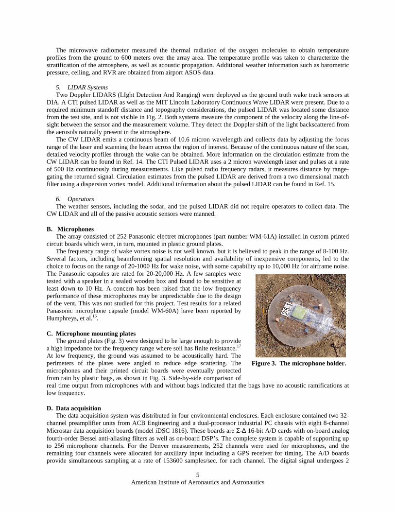
C. Microphone mounting plates The ground plates (Fig. 3) were designed to be large enough to provide

a high impedance for the frequency range where soil has finite resistance.17 At low frequency, the ground was assumed to be acoustically hard. The perimeters of the plates were angled to reduce edge scattering. The microphones and their printed circuit boards were eventually protected from rain by plastic bags, as shown in Fig. 3. Side-by-side comparison of real time output from microphones with and without bags indicated that the bags have no acoustic ramifications at low frequency.

D. Data acquisition The data acquisition system was distributed in four environmental enclosures. Each enclosure contained two 32-

channel preamplifier units from ACB Engineering and a dual-processor industrial PC chassis with eight 8-channel Microstar data acquisition boards (model iDSC 1816). These boards are Σ-∆ 16-bit A/D cards with on-board analog fourth-order Bessel anti-aliasing filters as well as on-board DSP’s. The complete system is capable of supporting up to 256 microphone channels. For the Denver measurements, 252 channels were used for microphones, and the remaining four channels were allocated for auxiliary input including a GPS receiver for timing. The A/D boards provide simultaneous sampling at a rate of 153600 samples/sec. for each channel. The digital signal undergoes 2

Figure 3. The microphone holder.


6

stages of filtering using 2 symmetric linear phase FIR filters implemented by the on-board DSP before down-sampling the data to a rate of 25600 samples/sec. for each channel. The data were buffered on the data acquisition boards and written to hard drives in the acquisition PCs. After a day or so, typically, the data were copied to a central backup PC and stored on removable hard drives for subsequent processing.

It was intended that all of the channels would be synchronized, but an unknown failure caused the data sets from the 8-channel boards to be offset from one board to the next by seemingly random shifts. The shifts remained constant for each run, but were different for the next run. A special data processing technique was developed to empirically determine the offset values for each data set, and these estimates were used to align the data for post processing.

Following Michel and Böhning,1 multiple gain settings were used during the flyover in an effort to collect airplane and wake acoustic data together. When an approaching airplane reached a reference point that was defined subjectively by a certain angle, the operator pressed “Start.” Data were acquired for 15 seconds or so with the preamplifiers set to a relatively low gain setting, and then the gain was increased for the remainder of the acquisition, which typically ran for 75 seconds. In post-processing, it was found that both gain settings were too high for many of the runs, leading to clipping. For wake data, the effect of the clipping was reduced by the filtering and decimation during the analysis.

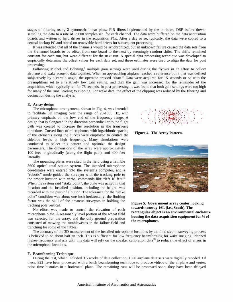
E. Array design The microphone arrangement, shown in Fig. 4, was intended

to facilitate 3D imaging over the range of 20-1000 Hz, with primary emphasis on the low end of the frequency range. A design that is elongated in the direction perpendicular to the flight path was created to increase the resolution in the transverse directions. Curved lines of microphones with logarithmic spacing of the elements along the curves were employed to control the sidelobe levels at high frequency. Many simulations were conducted to select this pattern and optimize the design parameters. The dimensions of the array were approximately 100 feet longitudinally (along the flight path), and 400 feet laterally.

The mounting plates were sited in the field using a Trimble 5600 optical total station system. The intended microphone coordinates were entered into the system’s computer, and a “robotic” mode guided the surveyor with the tracking pole to the proper location with verbal commands like “left 10 feet.” When the system said “stake point”, the plate was nailed in that location and the installed position, including the height, was recorded with the push of a button. The tolerance for the “stake point” condition was about one inch horizontally; the limiting factor was the skill of the amateur surveyors in holding the tracking pole vertical.

No effort was made to control the elevation of each microphone plate. A reasonably level portion of the wheat field was selected for the array, and the only ground preparation consisted of mowing the tumbleweeds in the fallow field and trenching for some of the cables.

The accuracy of the 3D measurement of the installed microphone locations by the final step in surveying process is believed to be about half an inch. This is sufficient for low frequency beamforming for wake imaging. Planned higher-frequency analysis with this data will rely on the speaker calibration data18 to reduce the effect of errors in the microphone locations.

F. Beamforming Technique During the test, which included 3.5 weeks of data collection, 1500 airplane data sets were digitally recoded. Of

these, 922 have been processed with a batch beamforming technique to produce videos of the airplane and vortex noise time histories in a horizontal plane. The remaining runs will be processed soon; they have been delayed

Figure 4. The Array Pattern.

Figure 5. Government array center, looking towards tunway 16L (i.e., South). The rectangular object is an environmental enclosure housing the data acquisition equipment for ¼ of the microphones.


7

because a new beamforming code has to be developed to deal with the alternative array design that was used. A few data sets have been selected for detailed examination. The techniques for this examination are described here.

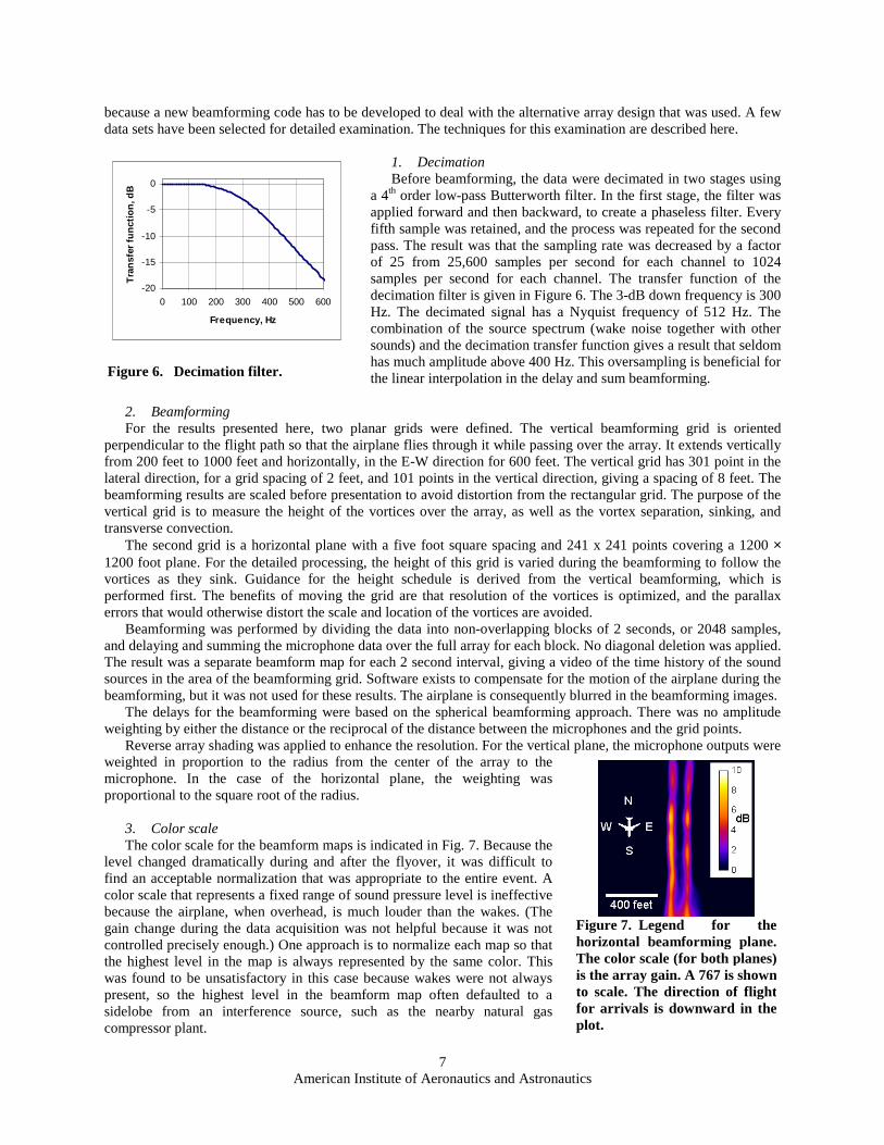
1. Decimation Before beamforming, the data were decimated in two stages using

a 4th order low-pass Butterworth filter. In the first stage, the filter was applied forward and then backward, to create a phaseless filter. Every fifth sample was retained, and the process was repeated for the second pass. The result was that the sampling rate was decreased by a factor of 25 from 25,600 samples per second for each channel to 1024 samples per second for each channel. The transfer function of the decimation filter is given in Figure 6. The 3-dB down frequency is 300 Hz. The decimated signal has a Nyquist frequency of 512 Hz. The combination of the source spectrum (wake noise together with other sounds) and the decimation transfer function gives a result that seldom has much amplitude above 400 Hz. This oversampling is beneficial for the linear interpolation in the delay and sum beamforming.

2. Beamforming For the results presented here, two planar grids were defined. The vertical beamforming grid is oriented

perpendicular to the flight path so that the airplane flies through it while passing over the array. It extends vertically from 200 feet to 1000 feet and horizontally, in the E-W direction for 600 feet. The vertical grid has 301 point in the lateral direction, for a grid spacing of 2 feet, and 101 points in the vertical direction, giving a spacing of 8 feet. The beamforming results are scaled before presentation to avoid distortion from the rectangular grid. The purpose of the vertical grid is to measure the height of the vortices over the array, as well as the vortex separation, sinking, and transverse convection.

The second grid is a horizontal plane with a five foot square spacing and 241 x 241 points covering a 1200 ×1200 foot plane. For the detailed processing, the height of this grid is varied during the beamforming to follow the vortices as they sink. Guidance for the height schedule is derived from the vertical beamforming, which is performed first. The benefits of moving the grid are that resolution of the vortices is optimized, and the parallax errors that would otherwise distort the scale and location of the vortices are avoided.

Beamforming was performed by dividing the data into non-overlapping blocks of 2 seconds, or 2048 samples, and delaying and summing the microphone data over the full array for each block. No diagonal deletion was applied. The result was a separate beamform map for each 2 second interval, giving a video of the time history of the sound sources in the area of the beamforming grid. Software exists to compensate for the motion of the airplane during the beamforming, but it was not used for these results. The airplane is consequently blurred in the beamforming images.

The delays for the beamforming were based on the spherical beamforming approach. There was no amplitude weighting by either the distance or the reciprocal of the distance between the microphones and the grid points.

Reverse array shading was applied to enhance the resolution. For the vertical plane, the microphone outputs were weighted in proportion to the radius from the center of the array to the microphone. In the case of the horizontal plane, the weighting was proportional to the square root of the radius.

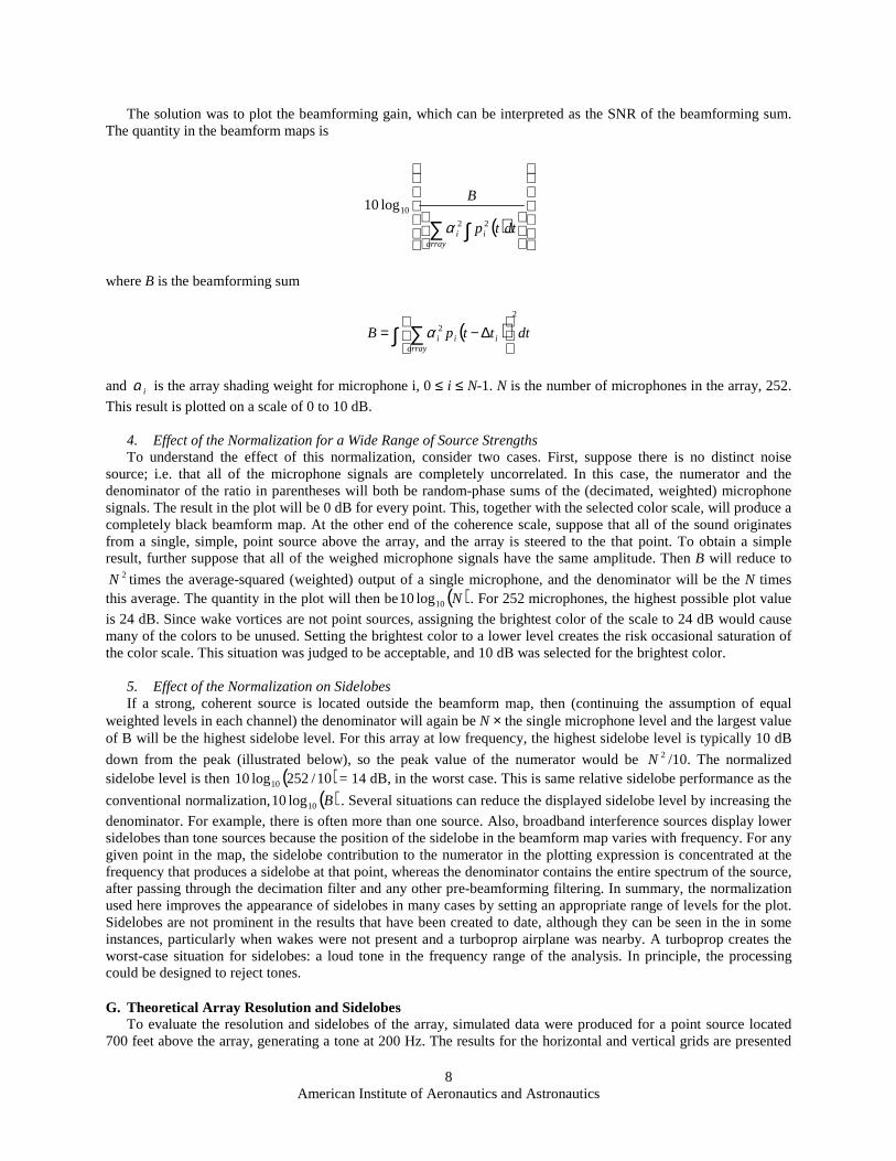
3. Color scale The color scale for the beamform maps is indicated in Fig. 7. Because the

level changed dramatically during and after the flyover, it was difficult to find an acceptable normalization that was appropriate to the entire event. A color scale that represents a fixed range of sound pressure level is ineffective because the airplane, when overhead, is much louder than the wakes. (The gain change during the data acquisition was not helpful because it was not controlled precisely enough.) One approach is to normalize each map so that the highest level in the map is always represented by the same color. This was found to be unsatisfactory in this case because wakes were not always present, so the highest level in the beamform map often defaulted to a sidelobe from an interference source, such as the nearby natural gas compressor plant.

Figure 7. Legend for the horizontal beamforming plane. The color scale (for both planes) is the array gain. A 767 is shown to scale. The direction of flight for arrivals is downward in the plot.

-20

-15

-10

-5

0

0 100 200 300 400 500 600

Frequency, Hz

Tra

nsf

erfu

nct

ion

,dB

Figure 6. Decimation filter.


8

The solution was to plot the beamforming gain, which can be interpreted as the SNR of the beamforming sum. The quantity in the beamform maps is

( )

∑ ∫

arrayii dttp

B

22

10log10

α

where B is the beamforming sum

( ) dtttpBarray

iii∫ ∑

∆−=

2

2α

and iα is the array shading weight for microphone i, 0 ≤ i ≤ N-1. N is the number of microphones in the array, 252.

This result is plotted on a scale of 0 to 10 dB.

4. Effect of the Normalization for a Wide Range of Source Strengths To understand the effect of this normalization, consider two cases. First, suppose there is no distinct noise

source; i.e. that all of the microphone signals are completely uncorrelated. In this case, the numerator and the denominator of the ratio in parentheses will both be random-phase sums of the (decimated, weighted) microphone signals. The result in the plot will be 0 dB for every point. This, together with the selected color scale, will produce a completely black beamform map. At the other end of the coherence scale, suppose that all of the sound originates from a single, simple, point source above the array, and the array is steered to the that point. To obtain a simple result, further suppose that all of the weighed microphone signals have the same amplitude. Then B will reduce to

2N times the average-squared (weighted) output of a single microphone, and the denominator will be the N times this average. The quantity in the plot will then be ( )N10log10 . For 252 microphones, the highest possible plot value

is 24 dB. Since wake vortices are not point sources, assigning the brightest color of the scale to 24 dB would cause many of the colors to be unused. Setting the brightest color to a lower level creates the risk occasional saturation of the color scale. This situation was judged to be acceptable, and 10 dB was selected for the brightest color.

5. Effect of the Normalization on Sidelobes If a strong, coherent source is located outside the beamform map, then (continuing the assumption of equal

weighted levels in each channel) the denominator will again be N × the single microphone level and the largest value of B will be the highest sidelobe level. For this array at low frequency, the highest sidelobe level is typically 10 dB

down from the peak (illustrated below), so the peak value of the numerator would be 2N /10. The normalized sidelobe level is then ( )10/252log10 10 = 14 dB, in the worst case. This is same relative sidelobe performance as the

conventional normalization, ( )B10log10 . Several situations can reduce the displayed sidelobe level by increasing the

denominator. For example, there is often more than one source. Also, broadband interference sources display lower sidelobes than tone sources because the position of the sidelobe in the beamform map varies with frequency. For any given point in the map, the sidelobe contribution to the numerator in the plotting expression is concentrated at the frequency that produces a sidelobe at that point, whereas the denominator contains the entire spectrum of the source, after passing through the decimation filter and any other pre-beamforming filtering. In summary, the normalization used here improves the appearance of sidelobes in many cases by setting an appropriate range of levels for the plot. Sidelobes are not prominent in the results that have been created to date, although they can be seen in the in some instances, particularly when wakes were not present and a turboprop airplane was nearby. A turboprop creates the worst-case situation for sidelobes: a loud tone in the frequency range of the analysis. In principle, the processing could be designed to reject tones.

G. Theoretical Array Resolution and Sidelobes To evaluate the resolution and sidelobes of the array, simulated data were produced for a point source located

700 feet above the array, generating a tone at 200 Hz. The results for the horizontal and vertical grids are presented


9

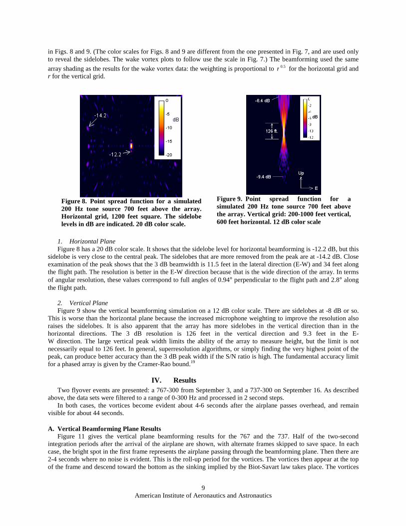
in Figs. 8 and 9. (The color scales for Figs. 8 and 9 are different from the one presented in Fig. 7, and are used only to reveal the sidelobes. The wake vortex plots to follow use the scale in Fig. 7.) The beamforming used the same

array shading as the results for the wake vortex data: the weighting is proportional to 5.0r for the horizontal grid and r for the vertical grid.

1. Horizontal Plane Figure 8 has a 20 dB color scale. It shows that the sidelobe level for horizontal beamforming is -12.2 dB, but this

sidelobe is very close to the central peak. The sidelobes that are more removed from the peak are at -14.2 dB. Close examination of the peak shows that the 3 dB beamwidth is 11.5 feet in the lateral direction (E-W) and 34 feet along the flight path. The resolution is better in the E-W direction because that is the wide direction of the array. In terms of angular resolution, these values correspond to full angles of 0.94° perpendicular to the flight path and 2.8° along the flight path.

2. Vertical Plane Figure 9 show the vertical beamforming simulation on a 12 dB color scale. There are sidelobes at -8 dB or so.

This is worse than the horizontal plane because the increased microphone weighting to improve the resolution also raises the sidelobes. It is also apparent that the array has more sidelobes in the vertical direction than in the horizontal directions. The 3 dB resolution is 126 feet in the vertical direction and 9.3 feet in the E- W direction. The large vertical peak width limits the ability of the array to measure height, but the limit is not necessarily equal to 126 feet. In general, superresolution algorithms, or simply finding the very highest point of the peak, can produce better accuracy than the 3 dB peak width if the S/N ratio is high. The fundamental accuracy limit for a phased array is given by the Cramer-Rao bound.19

IV. Results Two flyover events are presented: a 767-300 from September 3, and a 737-300 on September 16. As described

above, the data sets were filtered to a range of 0-300 Hz and processed in 2 second steps. In both cases, the vortices become evident about 4-6 seconds after the airplane passes overhead, and remain

visible for about 44 seconds.

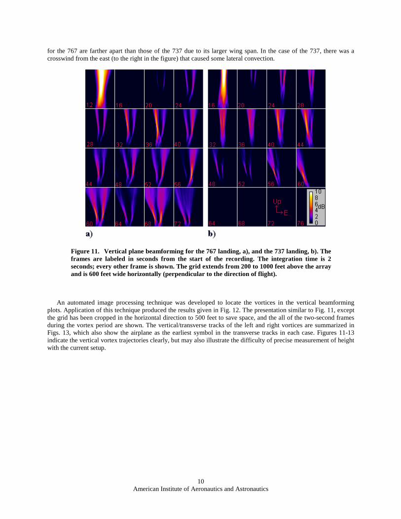
A. Vertical Beamforming Plane Results Figure 11 gives the vertical plane beamforming results for the 767 and the 737. Half of the two-second

integration periods after the arrival of the airplane are shown, with alternate frames skipped to save space. In each case, the bright spot in the first frame represents the airplane passing through the beamforming plane. Then there are 2-4 seconds where no noise is evident. This is the roll-up period for the vortices. The vortices then appear at the top of the frame and descend toward the bottom as the sinking implied by the Biot-Savart law takes place. The vortices

Figure 8. Point spread function for a simulated 200 Hz tone source 700 feet above the array. Horizontal grid, 1200 feet square. The sidelobe levels in dB are indicated. 20 dB color scale.

Figure 9. Point spread function for a simulated 200 Hz tone source 700 feet above the array. Vertical grid: 200-1000 feet vertical, 600 feet horizontal. 12 dB color scale


10

for the 767 are farther apart than those of the 737 due to its larger wing span. In the case of the 737, there was a crosswind from the east (to the right in the figure) that caused some lateral convection.

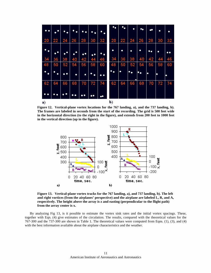
An automated image processing technique was developed to locate the vortices in the vertical beamforming plots. Application of this technique produced the results given in Fig. 12. The presentation similar to Fig. 11, except the grid has been cropped in the horizontal direction to 500 feet to save space, and the all of the two-second frames during the vortex period are shown. The vertical/transverse tracks of the left and right vortices are summarized in Figs. 13, which also show the airplane as the earliest symbol in the transverse tracks in each case. Figures 11-13 indicate the vertical vortex trajectories clearly, but may also illustrate the difficulty of precise measurement of height with the current setup.

Figure 11. Vertical plane beamforming for the 767 landing, a), and the 737 landing, b). The frames are labeled in seconds from the start of the recording. The integration time is 2 seconds; every other frame is shown. The grid extends from 200 to 1000 feet above the array and is 600 feet wide horizontally (perpendicular to the direction of flight).


11

Figure 12. Vertical-plane vortex locations for the 767 landing, a), and the 737 landing, b). The frames are labeled in seconds from the start of the recording. The grid is 500 feet wide in the horizontal direction (to the right in the figure), and extends from 200 feet to 1000 feet in the vertical direction (up in the figure).

Figure 13. Vertical-plane vortex tracks for the 767 landing, a), and 737 landing, b). The left and right vortices (from the airplanes’ perspective) and the airplane are labeled L, R, and A, respectively. The height above the array is z and easting (perpendicular to the flight path) from the array center is x.

By analyzing Fig 13, is it possible to estimate the vortex sink rates and the initial vortex spacings. These,

together with Eqn. (4) give estimates of the circulation. The results, compared with the theoretical values for the 767-300 and the 737-300 are shown in Table 1. The theoretical values were computed from Eqns. (1), (3), and (4) with the best information available about the airplane characteristics and the weather.


12

Table 1.

767 Array data

767 Theory

737 Array data

737 Theory

0b , ft. 125 122.7 81.0 74.5

0V , ft/s 7.85 6.2 9.6 7.74

Γ , m2/s 572.78 433.48 453.9 336.62

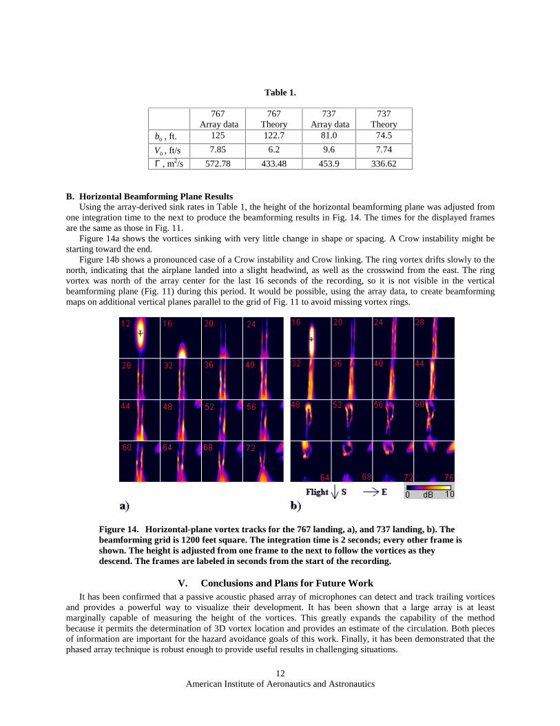
B. Horizontal Beamforming Plane Results Using the array-derived sink rates in Table 1, the height of the horizontal beamforming plane was adjusted from

one integration time to the next to produce the beamforming results in Fig. 14. The times for the displayed frames are the same as those in Fig. 11.

Figure 14a shows the vortices sinking with very little change in shape or spacing. A Crow instability might be starting toward the end.

Figure 14b shows a pronounced case of a Crow instability and Crow linking. The ring vortex drifts slowly to the north, indicating that the airplane landed into a slight headwind, as well as the crosswind from the east. The ring vortex was north of the array center for the last 16 seconds of the recording, so it is not visible in the vertical beamforming plane (Fig. 11) during this period. It would be possible, using the array data, to create beamforming maps on additional vertical planes parallel to the grid of Fig. 11 to avoid missing vortex rings.

Figure 14. Horizontal-plane vortex tracks for the 767 landing, a), and 737 landing, b). The beamforming grid is 1200 feet square. The integration time is 2 seconds; every other frame is shown. The height is adjusted from one frame to the next to follow the vortices as they descend. The frames are labeled in seconds from the start of the recording.

V. Conclusions and Plans for Future Work It has been confirmed that a passive acoustic phased array of microphones can detect and track trailing vortices

and provides a powerful way to visualize their development. It has been shown that a large array is at least marginally capable of measuring the height of the vortices. This greatly expands the capability of the method because it permits the determination of 3D vortex location and provides an estimate of the circulation. Both pieces of information are important for the hazard avoidance goals of this work. Finally, it has been demonstrated that the phased array technique is robust enough to provide useful results in challenging situations.


13

Data obtained during the Denver test will be further analyzed by several groups, including OptiNav, Volpe, NASA, and Florida Atlantic University, to explore the physics of aircraft wake generation and decay and, in particular, the acoustic signature generated by the vortex wake. Results from the analyses will be used to determine future efforts towards developing a viable wake detection sensor to help improve airport capacity.

References 1Michel, U. and P. Böhning, “Investigation of Aircraft Wake Vortices with Phased Microphone Arrays,” AIAA Paper 2002-

2501, Breckenridge, CO, June 2002. 2Cotton, W. and R. Williams., “PROJECT SOCRATES: A New Sensor Technology for Enhancement of Aviation Safety and

Capacity,” The 2002 FAA Airport Technology Conference, Atlantic City, NJ, May 5-8, 2002. 3Spalart, P. R., “Airplane Trailing Vortices” Ann. Rev. Fluid Mech., Vol. 30, 1998, pp. 107-38. 4Rossow, V.J., “Lift-Generated Vortex Wakes of Subsonic Transport Aircraft,” Progress in Aerospace Sciences, Pergamon,

Vol. 35, 1999, pp. 507-660. 5Gerz, T., F. Holzäpfel, and D. Darracq, “Commercial Aircraft Wake Vortices,” Progress in Aerospace Sciences, Pergamon,

Vol. 38, 2002, pp. 181-208. 6Chambers, J.R., Concept to Reality, Contributions of the NASA Langley Research Center to U.S. Civil Aircraft in the 1990s,

NASA SP-2003-4529, pp. 209-231. 7Prandtl, L, Essentials of Fluid Dynamics with Applications to Hydraulics, Aeronautics, Meteorology and other Subjects,

Hafner, New York, 1952. 8Hofbauer, T., and T. Gerz, “Shear-Layer Effects on the Dynamics of a Counter-Rotating Vortex Pair,” AIAA Paper 2000-

0758, Reno, NV, January 2000. 9Hardin, J., F. Y. Wang, and H. Wassaf, “Sound Generation by Aircraft Wake Vortices Interacting with the Ground Plane,”

AIAA Paper 2004-2881, Manchester, UK, May 2004. 10Crow, S. C., “Stability theory for a Pair of Trailing Vortices,” AIAA Paper No. 70-53, January 1970. 11Gerz, T. and F. Holzäpfel, “Wing-Tip Vortices, Turbulence, and the Distribution of Emissions,” AIAA Journal, Vol. 37,

No. 10, Oct. 1999, pp. 1270-1276. 12Howe, M. S., Theory of Vortex Sound, Cambridge University Press, Cambridge, UK, 2002. 13Müller, B., and H. C. Yee, “High Order Numerical Simulation of Sound Generated by the Kirchhoff Vortex,” Computing

and Visualization in Science, Vol. 4, No. 3, pp 197-204, Feb., 2002. 14Heinrichs, R. M. and T. J. Dasey., “Analysis of Circulation Data from a Wake Vortex Lidar,” AIAA Paper 97-0059, Reno,

NV, January 1997. 15Hannon, S. M., M. W. Phillips, J. A Thompson, and S. W Henderson, “Pulsed Coherent Lidar Wake Vortex Detection,

Tracking and Strength Estimate in Support of AVOSS,” NASA First Wake Vortex Dynamic Spacing Workshop - NASA CP-97-206235, 1997.

16Humphreys, W. M. Jr., C. H. Gerhold, A. J. Zuckerwar, G. C. Herring, and S. M. Bartram, “Performance Analysis of a Cost-Effective Electret Condenser Microphone Directional Array,” AIAA Paper 2003-3195, Hilton Head, SC, May 2003.

17Pierce, A. D., Acoustics: An Introduction to its Physical Principles and Applications, Acoustical Society of America, 1989, pp. 110-112.

18Doughery, R. P. , “Beamforming in Acoustic Testing,” Aeroacoustic Measurements, Edited by T. J. Mueller, Springer, Berlin, 2002, pp. 93-96.

19Stoica, P. and A. Nehorai, “MUSIC, Maximum Likelihood, and Cramer-Rao Bound,” IEEE Trans. ASSP-37, No. 5, May, 1989, pp. 720-741.

Documents

Aircraft Wake Vortex Measurements at Denver International ... · wake acoustics test at the Denver International Airport. The central instrument of the test was a large microphone