Airline Crew Scheduling with Time Windows and Plane-Count Constraints

This article was downloaded by: [129.173.72.87] On: 06 July 2014, At: 11:05Publisher: Institute for Operations Research and the Management Sciences (INFORMS)INFORMS is located in Maryland, USA

Transportation Science

Publication details, including instructions for authors and subscription information:http://pubsonline.informs.org

Airline Crew Scheduling with Time Windows and Plane-CountConstraintsDiego Klabjan, Ellis L. Johnson, George L. Nemhauser, Eric Gelman, Srini Ramaswamy,

To cite this article:Diego Klabjan, Ellis L. Johnson, George L. Nemhauser, Eric Gelman, Srini Ramaswamy, (2002) Airline Crew Scheduling with TimeWindows and Plane-Count Constraints. Transportation Science 36(3):337-348. http://dx.doi.org/10.1287/trsc.36.3.337.7831

Full terms and conditions of use: http://pubsonline.informs.org/page/terms-and-conditions

This article may be used only for the purposes of research, teaching, and/or private study. Commercial use orsystematic downloading (by robots or other automatic processes) is prohibited without explicit Publisher approval,unless otherwise noted. For more information, contact [email protected].

The Publisher does not warrant or guarantee the article’s accuracy, completeness, merchantability, fitness for aparticular purpose, or non-infringement. Descriptions of, or references to, products or publications, or inclusion of anadvertisement in this article, neither constitutes nor implies a guarantee, endorsement, or support of claims made ofthat product, publication, or service.

© 2002 INFORMS

Please scroll down for article—it is on subsequent pages

INFORMS is the largest professional society in the world for professionals in the fields of operations research, management science,and analytics.For more information on INFORMS, its publications, membership, or meetings visit http://www.informs.org

http://pubsonline.informs.org

http://dx.doi.org/10.1287/trsc.36.3.337.7831

http://pubsonline.informs.org/page/terms-and-conditions

http://www.informs.org

Airline Crew Scheduling with TimeWindows and Plane-Count Constraints

Diego Klabjan • Ellis L. Johnson • George L. Nemhauser •Eric Gelman • Srini Ramaswamy

Department of Mechanical and Industrial Engineering, University of Illinois at Urbana-Champaign,Urbana, Illinois, 61801

School of Industrial and Systems Engineering, Georgia Institute of Technology, Atlanta, Georgia 30332-0205School of Industrial and Systems Engineering, Georgia Institute of Technology, Atlanta, Georgia 30332-0205

Information Technology Services, American Airlines, Dallas-Ft. Worth Airport, Texas 75261-8616Research and Development, Information Services Division, United Airlines

[email protected] • [email protected] • [email protected] •[email protected] • [email protected]

Airline planning consists of several problems that are currently solved separately. Weaddress a partial integration of schedule planning, aircraft routing, and crew schedul-

ing. In particular, we provide more flexibility for crew scheduling while maintaining thefeasibility of aircraft routing by adding plane-count constraints to the crew-scheduling prob-lem. In addition, we assume that the departure times of flights have not yet been fixed andwe are allowed to move the departure time of a flight as long as it is within a given timewindow. We demonstrate that such a model yields solutions to the crew-scheduling problemwith significantly lower costs than those obtained from the traditional model.

Major United States airlines operate up to 2,500domestic flights per day. Due to the large number offlights, planning is complex and therefore is dividedinto several stages. Schedule development, i.e., whereand when to fly, comes first. Next is fleet assignment(FAM), where an assignment of fleets (equipmenttypes) to flights is made to maximize potential rev-enue. After FAM has been solved, the problems thatfollow decompose by fleet. In aircraft routing, an air-craft is assigned to each flight. Given a fleet andthe corresponding plane routes, the next step is crewscheduling, which consists of finding crew itinerariesor pairings. The last step, called rostering, is theassignment of crews to crew itineraries. Some recentliterature that presents the individual models is Haneet al. (1995) for fleet assignment, Clarke et al. (1997)for aircraft routing, Barnhart et al. (1999) for crewscheduling, and Gamache and Soumis (1998) for crew

rostering. Yu (1998) contains a collection of articles onairline planning and operations.

The five problems, schedule development, FAM,aircraft routing, crew scheduling, and rostering, aresolved separately. Ideally, all five problems shouldbe solved as a single problem, but this is not feasi-ble computationally. Here we take some steps towardan integrated approach. Our goal is to solve thecrew-scheduling problem, but we assume that crewscheduling is solved before aircraft routing and, inaddition, that the flight departure times are not fixed.To solve crew scheduling before aircraft routing, weadd additional constraints to the crew-schedulingmodel, which provide necessary conditions for theaircraft-routing problem to be feasible. Each flighthas a time window and the final departure timemust be within that time window. By assumingthat crew scheduling is solved before aircraft rout-ing, we are able to obtain solutions to the modified

0041-1655/02/3603/0337$05.001526-5447 electronic ISSN

Transportation Science © 2002 INFORMSVol. 36, No. 3, August 2002 pp. 337–348

Dow

nloa

ded

from

info

rms.

org

by [

129.

173.

72.8

7] o

n 06

Jul

y 20

14, a

t 11:

05 .

For

pers

onal

use

onl

y, a

ll ri

ghts

res

erve

d.

KLABJAN, JOHNSON, NEMHAUSER, GELMAN, AND RAMASWAMYAirline Crew Scheduling

crew-scheduling problem that are significantly bet-ter than solutions obtained by using the traditionalcrew-scheduling model. The retimed flights shouldnot have a big impact on the quality of the sched-ule and the FAM solution because the time windowsconsidered are small.

The rest of the paper is organized as follows.In §1 we explain the constraints that have to beadded to the crew-scheduling problem to meet plane-count constraints. The time window aspect of pairingsis described in §2. Section 3 describes the solu-tion methodology. The resulting problem is a set-partitioning problem with side constraints, and weshow the extra steps required to account for the sideconstraints. Computational results are presented in§4. We conclude the introduction with brief descrip-tions of the fleet assignment, the aircraft-routing prob-lems, and the crew-scheduling problems.

Major United States airlines domestic operationsare based on a hub-and-spoke network. High activ-ity airports are called hubs and low activity airportsare called spokes. After the schedule has been built,FAM is solved. FAM has two fundamental sets ofconstraints: flow conservation and plane count. Flowconservation is represented by a time-space networkin which there are arcs for each flight leg or segment,i.e., a nonstop flight. Therefore, an arc specifies twoevents: a departure and an arrival. The constraints that aFAM solution cannot use more aircraft than there existin a fleet are modeled by introducing ground arcsand the associated variables. A ground arc representsa connection between two consecutive events with noflight activity in between. Each fleet has its own setof ground-arc variables. The nonnegative ground-arcvariable counts the number of planes in the fleet onthe ground in the time interval defined by the arc. Wecall the value of such a variable the ground-arc value.For each fleet, the flow-conservation constraints statethat the number of planes on the ground plus thenumber of planes arriving must be equal to the num-ber of planes on the ground in the next time intervalplus the number of planes departing. The total num-ber of planes in a fleet is the sum of all the ground-arcvalues of those arcs at a specified point in time, e.g.,midnight, plus those aircraft that are in the air.

An aircraft route is a sequence of flights that areflown by the same aircraft, and a rotation or a routingis a set of aircraft routes that partition all the flightsin the schedule. Given a fleet, the aircraft-routing prob-lem is to find a routing that satisfies the plane-countconstraints and other constraints mainly related tomaintenance, e.g., Gu et al. (1994) and Clarke et al.(1997). We say that a routing is plane-count feasible if itsatisfies the plane-count constraints.

A plane-turn time is the time needed for a plane tobe ready for the next flight after arriving at a gate.We denote by minTurn the minimum plane-turn time,which can depend on various factors such as the sta-tion and local time, but for simplicity we assume it isa constant. We use a default value minTurn= 30 min-utes. In the sequel, all times are given in minutes.

A duty is a working day of a crew that consistsof a sequence of flights and is subject to FAA andcompany rules. Among other rules, there is a min-imum and maximum connection time between twoconsecutive flights in the duty. A connection withina duty is called a sit connection. We denote by min-Sit the minimum sit-connection time. The defaultvalue is minSit = 45. The minimum sit-connectiontime requirement can be violated only if the crew fol-lows the plane turn, i.e., they do not change planes.The cost of a duty (measured in minutes) is the maxi-mum of three quantities: the flying time, a fraction ofthe elapsed time, and the duty minimum guaranteedpay.

Crew bases are designated stations where crewsmust start their first duty and end their last duty. Apairing is a sequence of duties, starting and ending ata crew base and with the elapsed time no more thana week. A connection between two duties is called anovernight connection or layover. We refer to the time ofa layover as the rest. Similar to sit-connection times,there is a lower and an upper bound on the rest. Wedenote by minRest the minimum allowed rest time(minRest= 620 for our data).

The cost of a pairing is also the maximum of threequantities: the sum of the duty costs in the pairing, afraction of the time away from base, and a minimumguaranteed pay times the number of duties. The excesscost of a pairing is defined as the cost minus the flyingtime of the pairing. Note that the excess cost is always

338 Transportation Science/Vol. 36, No. 3, August 2002

Dow

nloa

ded

from

info

rms.

org

by [

129.

173.

72.8

7] o

n 06

Jul

y 20

14, a

t 11:

05 .

For

pers

onal

use

onl

y, a

ll ri

ghts

res

erve

d.


nonnegative. The flight time credit (FTC) of a pairing isthe excess cost times 100 divided by the flying time,i.e., the excess time measured as a percentage of flyingtime. A pairing is also subject to many FAA rules.

The airline crew-scheduling problem is to find a setof pairings that partition all of the segments and min-imize excess cost. The daily airline crew-schedulingproblem is the crew-scheduling problem with theassumption that each leg is flown every day of theweek. Because in practice, a small number of legs arenot operated during weekends, a daily solution needsto be modified somewhat to obtain a weekly solution.This paper deals exclusively with the daily problem.Traditionally, a crew-scheduling problem is modeledas the set-partitioning problem

min�cx � Ax = 1 x binary� (1)

where each variable corresponds to a pairing; aij =1 if leg i is in pairing j and 0 otherwise, and cj isthe excess cost of pairing j. Note that for the dailyproblem, a pairing cannot cover a leg more than oncebecause pairings are repeated in the time horizon.

The problem is difficult because the number of pair-ings, i.e., columns, can be extremely large. The num-ber of pairings varies from about 200,000 for smallfleets, to about a billion for medium-sized fleets, andto billions for large fleets. Furthermore, because thecost function of a pairing is nonlinear and the legal-ity rules are complex, it is challenging to performdelayed column generation, i.e., generating columnsonly as they are needed in the optimization algorithm.

There have not been many attempts to integrateplanning stages. Barnhart et al. (1998) present amodel that integrates, to some extent, FAM and crewscheduling. The model has a very large number ofconstraints and therefore is hard to solve. Rexing(1998) presents a FAM model with time windows. Hisapproach significantly differs from ours in the waythe columns are generated. He discretizes the timewindow intervals, whereas we generate columns onthe fly without discretizing time windows. Anotherintegration of the FAM model and time windows ispresented in Desaulniers et al. (1997). They use a set-partitioning model with side constraints and solveproblems with up to 400 flights. Barnhart et al. (1998)

discuss the integration of FAM and aircraft routing byconsidering strings of flights.

Recently Cordeau et al. (2001) proposed a modelthat fully integrates crew scheduling and aircraft rout-ing because it produces a feasible crew schedule andfeasible aircraft routing. Their model is solved withbranch-and-price, where at each node of the tree themaster problem is optimized with Benders decompo-sition. They report computational results with fleetscontaining up to 500 flights and a spoke-to-spokeflight network, but it is not clear if the approachis computationally tractable on hub-and-spoke flightnetworks with many crew bases.

There are also approaches that integrate crew andvehicle scheduling in urban mass transit systems.Haase et al. (1998) present a model that minimizes thecrew cost and the number of vehicles. Their model isthe set-partitioning model with side constraints and itis solved with a branch-and-cut-and-price algorithm.Our model is similar, except that in our applicationthe number of resources, i.e., aircraft, at any giventime in the time horizon is given by FAM. Frelinget al. (2000) propose a model that links the crew-scheduling formulation with the vehicle-schedulingformulation. The model preserves the flow of thevehicles, but it does not try to minimize the num-ber of vehicles. Their model resembles the model inCordeau et al. (2001). Other references on urban masstransit systems can be found in these two papers.

1. Plane-Count ConstraintsEven though the difference between minSit (45 min-utes) and minTurn (30 minutes) is relatively small,judiciously choosing the plane turns can significantlyaffect the quality of crew scheduling. We performedan experiment on a small fleet consisting of 123legs. Table 1 shows the effect of the minimum sit-connection time on the excess cost. The last columnrefers to the problem with minSit = 45 and a givenaircraft routing, i.e., the approach used in current

Table 1 The Impact of the Minimum Sit-Time on FTC

minSit 30 35 40 45 Turns

FTC 8.4 8.5 10 12.5 11

Transportation Science/Vol. 36, No. 3, August 2002 339

Dow

nloa

ded

from

info

rms.

org

by [

129.

173.

72.8

7] o

n 06

Jul

y 20

14, a

t 11:

05 .

For

pers

onal

use

onl

y, a

ll ri

ghts

res

erve

d.


methodology. The remaining columns show the objec-tive value if the minimum sit-connection time is setto a given number and aircraft routing is neglected.Clearly, it is advantageous to have a minimum sit-connection time of 30 minutes. The experiment alsoindicated that a different routing can significantlyreduce the FTC.

The current methodology finds a routing first andthen solves the crew-scheduling problem. A modelthat considers crew scheduling as well as aircraftrouting would require variables for strings as wellas pairings, resulting in a larger formulation. How-ever, because our primary objective is to solve thecrew-scheduling problem, we will develop a formu-lation that incorporates the necessary aircraft con-straints without using string variables.

Therefore, instead of completely combining the twoproblems, we solve them sequentially but reverse theorder in which they are solved. The advantage ofthis approach is that the crew cost is high and theimpact of a routing on the crew cost can be substan-tial. Furthermore, the routing problem is primarily afeasibility problem and generally has many feasiblesolutions. In the remainder of the paper we assumethat a routing is not given. Because we do not knowthe plane turns, any pairing having sit connectionsshorter than minSit can be a feasible pairing assumingthat the plane turns are implied by the pairing.

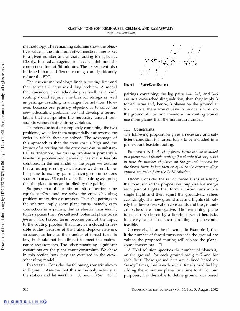
Suppose that the minimum sit-connection timeequals minTurn and we solve the crew-schedulingproblem under this assumption. Then the pairings inthe solution imply some plane turns, namely, eachconnection in a pairing that is shorter than minSit,forces a plane turn. We call such potential plane turnsforced turns. Forced turns become part of the inputto the routing problem that must be included in fea-sible routes. Because of the hub-and-spoke networkstructure, as long as the number of forced turns islow, it should not be difficult to meet the mainte-nance requirements. The other remaining significantconstraints are the plane-count constraints. We showin this section how they are captured in the crew-scheduling model.Example 1. Consider the following scenario shown

in Figure 1. Assume that this is the only activity atthe station and let minTurn = 30 and minSit = 45. If

Figure 1 Plane-Count Example

pairings containing the leg pairs 1–4, 2–5, and 3–6are in a crew-scheduling solution, then they imply 3forced turns and, hence, 3 planes on the ground at8:31. Hence, there would have to be one aircraft onthe ground at 7:59, and therefore this routing woulduse more planes than the minimum number.

1.1. ConstraintsThe following proposition gives a necessary and suf-ficient condition for forced turns to be included in aplane-count feasible routing.

Proposition 1. A set of forced turns can be includedin a plane-count feasible routing if and only if at any pointin time the number of planes on the ground imposed bythe forced turns is less than or equal to the correspondingground-arc value from the FAM solution.

Proof. Consider the set of forced turns satisfyingthe condition in the proposition. Suppose we mergeeach pair of flights that form a forced turn into asingle flight and then adjust the ground-arc valuesaccordingly. The new ground arcs and flights still sat-isfy the flow-conservation constraints and the ground-arc values are nonnegative. The remaining planeturns can be chosen by a first-in, first-out heuristic.It is easy to see that such a routing is plane-countfeasible.

Conversely, it can be shown as in Example 1, thatif the number of forced turns exceeds the ground-arcvalues, the proposed routing will violate the plane-count constraints. �

A FAM solution specifies the number of planes bgon the ground, for each ground arc g ∈ G and foreach fleet. These ground arcs are defined based on“ready” times, that is each arrival time is modified byadding the minimum plane turn time to it. For ourpurposes, it is desirable to define ground arcs based


Dow

nloa

ded

from

info

rms.

org

by [

129.

173.

72.8

7] o

n 06

Jul

y 20

14, a

t 11:

05 .

For

pers

onal

use

onl

y, a

ll ri

ghts

res

erve

d.


on the original schedule, instead of on the “ready”times. Given the ground-arc values from a FAM solu-tion, it is easy to compute ground-arc values based onour definition.

In a daily FAM model, where each flight leg isflown every day, the ground arcs G correspond totime intervals within a given 24 hour period. For aground arc g ∈ G we use the notation g+d to repre-sent that the ground arc g is shifted by d days in aweekly horizon. We say that a pairing includes a groundarc if there is a forced turn within the pairing thatcontains the time interval represented by the groundarc. Let P be the set of pairings that can be generatedfrom legs in the schedule based on the minimum sit-connection time of minTurn minutes. For each g ∈ G,let Pg ⊂ P be the set of all pairings having a forcedturn that includes one of g g+1 � � � g+6. Because aground arc with length greater than or equal to min-Sit has Pg = �, we only need to consider the subsetG′ ⊆ G whose elements have length less than minSit.Note that a pairing including g and g+d contributestwo forced turns because it is repeated in the weeklyhorizon. For each g ∈ G′ and for each p ∈ Pg , defineapg to be the number of times the pairing p includesone of g g+1 � � � g+6. The plane-count constraintscan be written as

∑p∈Pg apgxp ≤ bg .

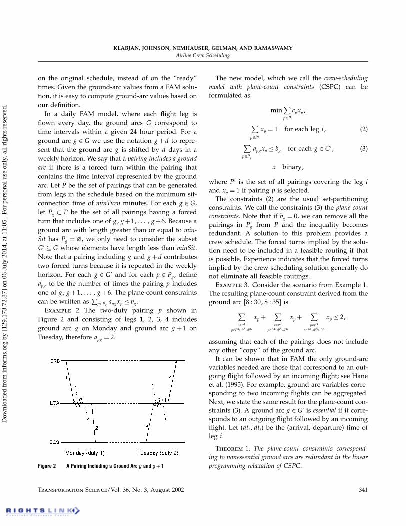
Example 2. The two-duty pairing p shown inFigure 2 and consisting of legs 1, 2, 3, 4 includesground arc g on Monday and ground arc g+ 1 onTuesday, therefore apg = 2.

Figure 2 A Pairing Including a Ground Arc g and g+1

The new model, which we call the crew-schedulingmodel with plane-count constraints (CSPC) can beformulated as

min∑p∈P

cpxp

∑p∈Pi

xp = 1 for each leg i (2)

∑p∈Pg

apgxp ≤ bg for each g ∈G′ (3)

x binary

where Pi is the set of all pairings covering the leg iand xp = 1 if pairing p is selected.

The constraints (2) are the usual set-partitioningconstraints. We call the constraints (3) the plane-countconstraints. Note that if bg = 0, we can remove all thepairings in Pg from P and the inequality becomesredundant. A solution to this problem provides acrew schedule. The forced turns implied by the solu-tion need to be included in a feasible routing if thatis possible. Experience indicates that the forced turnsimplied by the crew-scheduling solution generally donot eliminate all feasible routings.Example 3. Consider the scenario from Example 1.

The resulting plane-count constraint derived from theground arc �8 � 30 8 � 35� is∑

p∈P1

p∈P4∪P5∪P6

xp+∑p∈P2

p∈P4∪P5∪P6

xp+∑p∈P3

p∈P4∪P5∪P6

xp ≤ 2

assuming that each of the pairings does not includeany other “copy” of the ground arc.

It can be shown that in FAM the only ground-arcvariables needed are those that correspond to an out-going flight followed by an incoming flight; see Haneet al. (1995). For example, ground-arc variables corre-sponding to two incoming flights can be aggregated.Next, we state the same result for the plane-count con-straints (3). A ground arc g ∈G′ is essential if it corre-sponds to an outgoing flight followed by an incomingflight. Let �ati dti� be the (arrival, departure) time ofleg i.

Theorem 1. The plane-count constraints correspond-ing to nonessential ground arcs are redundant in the linearprogramming relaxation of CSPC.


Dow

nloa

ded

from

info

rms.

org

by [

129.

173.

72.8

7] o

n 06

Jul

y 20

14, a

t 11:

05 .

For

pers

onal

use

onl

y, a

ll ri

ghts

res

erve

d.


As a result of this theorem (the proof is given inKlabjan 1999), the number of necessary plane-countconstraints can be significantly reduced to only thosethat correspond to essential ground arcs. Their addi-tion to the standard crew-scheduling model shouldnot cause significant computational difficulties.

2. Time WindowsHere we assume that the schedule is not yet fixed,in the sense that we are allowed to make very smallchanges in the departure time of each leg. For obvi-ous reasons it would not make sense to consider “big”changes in departure times. For the remainder of thepaper let 2w be the size of the time window in min-utes. Namely, the revised departure time of a leg i

must be in the time interval �dti−w dti+w�. The off-set of leg i is the revised departure time minus theoriginal departure time dti. A typical value for w is5 or 10 minutes. We assume a default value w = 5.For simplicity, we assume that the window size doesnot depend on the leg index but the approach can beeasily generalized to handle such a dependency.

The output of the crew-scheduling problem with timewindows is a set of departure offsets and a set ofpairings that partition the legs and are feasible basedon the retimed schedule. The flexibility in departuretimes should allow pairings that are infeasible basedon the original schedule to become feasible. For exam-ple, if two legs are separated by 20 minutes, theycan be part of a pairing if the departure time of eachone of them is adjusted by five minutes in the finalretimed schedule.

Therefore, we expect better objective values to bemostly because of the increased number of feasiblepairings rather than because of the change in the costof a pairing if its legs are perturbed. In addition, tocapturing more short-sit connections, shorter layovertimes can increase the number of possible pairingsas well. Many pairings that are disregarded becausethey violate the 8-in-24 rule might become feasible ifwe retime the legs. Additional pairings can also becaptured by extending the maximum sit-connectiontime by 2w, but we do not address this possibilityhere because such a duty would have a high cost and,hence, it is unlikely that it would be part of a good

solution. However, the techniques presented can beeasily extended to allow this extension.

We define a duty as a sequence of flights that sat-isfies all the FAA and company rules based on theoriginal schedule and the modified pairing feasibilityparameters minSit = minSit− 2w and the maximumduty elapsed time is increased by 2w.

A feasible pairing with respect to a given feasibility ruleis a sequence of duties, starting and ending at a crewbase, together with offsets of the legs such that thegiven feasibility rule is satisfied with respect to thedeparture times defined by the offsets. In what fol-lows a pairing is a feasible pairing with respect to allof the feasibility rules, specifically the minimum andthe maximum sit-and rest-connection times, the max-imum duty elapsed time, and the 8-in-24 rule, anda single set of offsets for all of the feasibility rules.Assume we modify the following pairing feasibilityparameters: minSit=minSit−2w, minRest=minRest−2w, the maximum duty elapsed time is increased by2w, and the minimum allowed compensatory rest isreduced by 2w. A potential pairing is a sequence ofduties, starting and ending at a crew base, such thatall of the feasibility rules are satisfied based on theoriginal schedule and the modified pairing feasibilityparameters. Note that every pairing is also a potentialpairing, but the converse is not true. A duty consistingof two consecutive connections of 20 and 25 minutescannot be part of a pairing because there is no way toretime the three involved legs to meet the minimumsit-connection requirement of 30 minutes; however, itcan be part of a potential pairing. On the other hand, aduty with two consecutive 20 and 30 minute connec-tions can be part of a pairing because we can retimethe three legs to have the sit-connection times longerthan 30 minutes.

We generate potential pairings, and during the gen-eration we compute new departure times of legs ina potential pairing such that at the end we producea pairing. If a partial potential pairing cannot beextended, it is pruned. With the parameters givenabove, every pairing can be generated. Because of thehub-and-spoke flight network structure and severalcrew bases for large fleets, all of the pairings cannotbe generated in a reasonable amount of time. Instead,


Dow

nloa

ded

from

info

rms.

org

by [

129.

173.

72.8

7] o

n 06

Jul

y 20

14, a

t 11:

05 .

For

pers

onal

use

onl

y, a

ll ri

ghts

res

erve

d.


we generate subsets of random pairings as proposedin Klabjan et al. (2001).

There are two possible approaches to pairing gen-eration: One generates pairings directly from legs andthe other generates duties first and then pairings areconstructed from duties. For a more comprehensivediscussion of pairing generation see Klabjan (1999).Here we generate pairings from duties by depth-firstsearch.

2.1. Generating Feasible PairingsWe first show how to generate feasible pairings withrespect to connection times and duty elapsed times.For the time being we ignore the 8-in-24 rule.

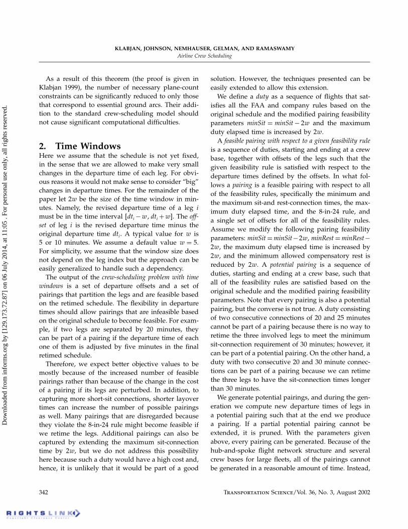
For a potential pairing having l legs, let ci be theconnection time between the ith and the �i+1�th legin the original schedule, i= 1 � � � l−1. Note that ci ≥minTurn− 2w or ci ≥ minRest− 2w depending on thetype of connection. Define mi i = 1 � � � l− 1 to beminTurn if the connection i is a sit connection andminRest otherwise.Example 4. Consider the potential pairing in

Figure 3 depicted in bold. The connection times arelisted next to the connections. Legs 3, 4, and 5 can beretimed to make feasible connections and the same istrue for Legs 2, 3, and 4; however, we can not retimeLegs 2, 3, 4, and 5 to form feasible connections. To seethis, we can attempt to “stretch” the connections start-ing with Leg 2. We can move it five minutes earlier(dashed flight legs in the figure) and then try to makethe next connection as short as possible. We proceedin this manner until we reach Leg 5, which wouldhave to be moved by six minutes, thus violating thetime window.

A formal reason for not being able to retime Legs2, 3, 4, and 5 is that the connection time deficit∑4

i=2�ci−mi� = −11 cannot be compensated for by

Figure 3 An Example of a Potential Pairing that Cannot Be Retimed

moving the departure time of the second Leg fiveminutes earlier and the departure time of the fifth legfive minutes later. No matter how large the connec-tion times are between the Legs 1, 2 and 5, 6, we can-not retime the whole potential pairing. The potentialpairing in the figure is not a pairing.

We start with a proposition that addresses the con-nection times issue. The proposition is presented in amore general setting, namely, window sizes dependon the leg index, which will be needed later.

Proposition 2. Let the sequence of legs in a pairingbe given by �1 2 � � � l�, and assume that each leg i hasa window size wi and that ci ≥ mi −wi −wi+1 for eachindex i. The potential pairing is a feasible pairing withrespect to connection times if and only if

i∑j=s�cj −mj�+ws+wi+1 ≥ 0 (4)

for all 1 ≤ s ≤ i ≤ l−1.

Proof. We first prove the necessity of (4). Assumethat each leg has an offset xj such that the feasiblepairing satisfies connection time requirements basedon the offsets, i.e., the departure time of the leg jis dtj + xj , −wj ≤ xj ≤ wj . Then mj ≤ cj + xj+1 − xj foreach 1 ≤ j ≤ l−1. Note that the right-hand side of theinequality is the connection time of the pairing and,hence, by definition is larger than mj . Summing theinequalities from s to i and using the time windowbounds, we get the claim.

The sufficiency is proved algorithmically by con-structing leg offsets such that the new departure timesare as early as possible and they yield a feasible pair-ing with respect to connection times.

Algorithm 1 computes a set of offsets x. We claimthat the given offsets satisfy the time window restric-tions and the minimum connection time require-ments.

It is easy to see that the computed connection timeis always greater than or equal to mi−1. We still needto show that xi is within the time window usingthe assumption given in the proposition. Clearly, xi ≥−wi. By induction it follows that either xi = −wi

or there is an index s 1 ≤ s ≤ i− 1 such that xi =∑i−1j=s �mj− cj�−ws . In the first case, xi ≤wi. In the sec-

ond case, the claim follows directly from the assump-tion in the proposition. �


Dow

nloa

ded

from

info

rms.

org

by [

129.

173.

72.8

7] o

n 06

Jul

y 20

14, a

t 11:

05 .

For

pers

onal

use

onl

y, a

ll ri

ghts

res

erve

d.


Note that the proof of the proposition also estab-lishes a linear time algorithm for computing the off-sets or detecting infeasibility. An infeasibility occurswhenever a computed offset is not within the timewindow.

We have already indicated that the duties are gen-erated first. Consider a duty d having k legs and apotential pairing containing the duty. No matter whatthe offsets of the first and the last legs of the duty inthe pairing are, the inequalities

∑ij=s�cj −minTurn�+

2w ≥ 0 must hold for all 2 ≤ s ≤ i ≤ k− 2. So allthe duties violating one of these inequalities must beremoved.

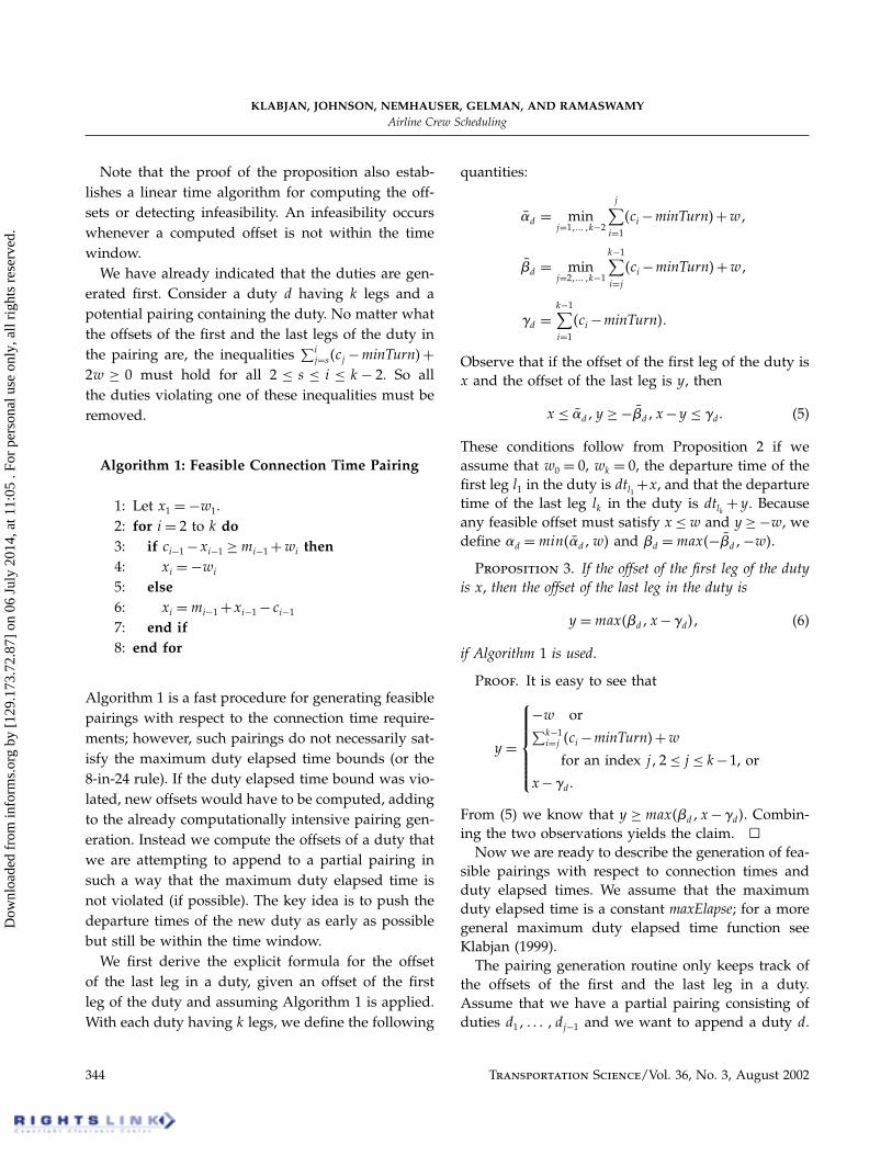
Algorithm 1: Feasible Connection Time Pairing

1: Let x1 =−w1.2: for i = 2 to k do3: if ci−1 −xi−1 ≥mi−1 +wi then4: xi =−wi

5: else6: xi =mi−1 +xi−1 − ci−1

7: end if8: end for

Algorithm 1 is a fast procedure for generating feasiblepairings with respect to the connection time require-ments; however, such pairings do not necessarily sat-isfy the maximum duty elapsed time bounds (or the8-in-24 rule). If the duty elapsed time bound was vio-lated, new offsets would have to be computed, addingto the already computationally intensive pairing gen-eration. Instead we compute the offsets of a duty thatwe are attempting to append to a partial pairing insuch a way that the maximum duty elapsed time isnot violated (if possible). The key idea is to push thedeparture times of the new duty as early as possiblebut still be within the time window.

We first derive the explicit formula for the offsetof the last leg in a duty, given an offset of the firstleg of the duty and assuming Algorithm 1 is applied.With each duty having k legs, we define the following

quantities:

�d = minj=1 �� k−2

j∑i=1

�ci−minTurn�+w

d = minj=2 �� k−1

k−1∑i=j�ci−minTurn�+w

!d =k−1∑i=1

�ci−minTurn��

Observe that if the offset of the first leg of the duty isx and the offset of the last leg is y, then

x ≤ �d y ≥− d x−y ≤ !d� (5)

These conditions follow from Proposition 2 if weassume that w0 = 0, wk = 0, the departure time of thefirst leg l1 in the duty is dtl1 +x, and that the departuretime of the last leg lk in the duty is dtlk + y. Becauseany feasible offset must satisfy x ≤w and y ≥−w, wedefine �d =min��d w� and d =max�− d −w�.

Proposition 3. If the offset of the first leg of the dutyis x, then the offset of the last leg in the duty is

y =max� d x−!d� (6)

if Algorithm 1 is used.

Proof. It is easy to see that

y =

−w or∑k−1i=j �ci−minTurn�+w

for an index j 2 ≤ j ≤ k−1, or

x−!d�From (5) we know that y ≥max� d x−!d�. Combin-ing the two observations yields the claim. �

Now we are ready to describe the generation of fea-sible pairings with respect to connection times andduty elapsed times. We assume that the maximumduty elapsed time is a constant maxElapse; for a moregeneral maximum duty elapsed time function seeKlabjan (1999).

The pairing generation routine only keeps track ofthe offsets of the first and the last leg in a duty.Assume that we have a partial pairing consisting ofduties d1 � � � dj−1 and we want to append a duty d.


Dow

nloa

ded

from

info

rms.

org

by [

129.

173.

72.8

7] o

n 06

Jul

y 20

14, a

t 11:

05 .

For

pers

onal

use

onl

y, a

ll ri

ghts

res

erve

d.


Let �x1 y1� � � � �xj−1 yj−1� be the computed offsets.We want to derive the offsets �xj yj� such that the par-tial pairing extended with the duty d satisfies the min-imum and maximum sit- and rest-connection times,and the maximum duty elapsed time based on thecomputed offsets.

We would like to avoid backtracking when recom-puting the new offsets of the already appendedduties. To achieve this, we generate the utmost leftpairing. A pairing is the utmost left pairing if it isa pairing based on offsets x1 � � � xj , and for anytime t and index i i ≤ j, the pairing with offsetsx1 � � � xi−1 xi−t xi+1 � � � xj violates either the maxi-mum duty elapsed time bound or a minimum connec-tion time limit. Hence, as soon as we move a depar-ture time one time unit earlier, the pairing violatesone of the two feasibility rules.

In addition to computing the new offsets �xj yj� insuch a way that the new partial pairing satisfies thefeasibility rules, we need to preserve the utmost leftproperty. We assume that the current partial pairingis the utmost left one. Let mj−1 be the minimum resttime. Define

#j ={−w if cj−1 −yj−1 ≥mj−1 +w mj−1 +yj−1 − cj−1 otherwise.

Note that #j is determined by performing one stepof Algorithm 1. Combining the above definition andthe inequalities (5), the new offsets have to satisfy theinequalities

#j ≤ xj ≤ �d (7)

d ≤ yj ≤w (8)

xj −yj ≤ !d� (9)

The above inequalities guarantee that the new par-tial pairing based on the offsets will have connectiontimes that are bigger than the required minimum. Westill need to take care of the maximum duty elapsedtime and the utmost left property. Assume that ed isthe elapsed time of the duty d based on the originalschedule, and let ed be the elapsed time of the retimedduty.

Then it is clear that ed = ed − xj + yj . The elapsedtime ed has to be smaller than or equal to maxElapse.Hence, we get an additional inequality

ed ≤ xj −yj (10)

where ed = ed−maxElapse. The new offsets have to sat-isfy the system of inequalities (7)–(10), denoted by Q.

We claim that if system Q is infeasible, then wecannot append the duty d. Suppose there were aset of offsets �x1 y1� � � � �xj yj� such that the partialpairing �d1 � � � dj−1 d� satisfies the feasibility rules.Then the offsets xj and yj have to satisfy (8), (9), and(10). Because xj ≤ �d, it must be the case that xj < #j .Because of the definition of #j , it follows that yj−1 <

yj−1. But this contradicts the utmost left property ofthe partial pairing and the computed offsets.

Assume now that system Q is feasible. We canexplicitly compute a solution to the system that min-imizes xj using Fourier-Motzkin elimination (e.g.,Schrijver 1986) given by

xj = max�#j d+ ed� (11)

yj = max� d x−!d�� (12)

This solution has the smallest xj and the corre-sponding yj is the one listed in Proposition 3. If westart with the offset xj and apply Algorithm 1, thenthe resulting yj is given by (12). Clearly the algorithmproduces the utmost left sequence of offsets. Hence,the values given by (11) and (12) maintain the prop-erty of being the utmost left.

To summarize, we compute the values xj and yjfrom the formulas (11) and (12) and then checkinequalities (7)–(10). If at least one is violated, thenthe duty d is discarded. Otherwise, we append theduty d and impose the corresponding offsets �xj yj�.

In the United States, the FAA requires that pairingssatisfy the 8-in-24 rule, which says that if in a 24 hourtime window there is more than eight hours of flying,then the next rest, called a compensatory rest, must belonger than a given limit. Different flight departuretimes can cause a violation of the rule and, therefore,care has to be taken when time windows are present.The treatment of the 8-in-24 rule and time windowscan be done efficiently as described in Klabjan (1999).

3. Solution MethodologyWe outline the overall methodology of integrating theplane-count constraints and time windows into thecrew-scheduling model.


Dow

nloa

ded

from

info

rms.

org

by [

129.

173.

72.8

7] o

n 06

Jul

y 20

14, a

t 11:

05 .

For

pers

onal

use

onl

y, a

ll ri

ghts

res

erve

d.


(1) We generate potential pairings based on theoriginal schedule, but with some pairing feasibilityparameters modified. Namely, the minimum sit andlayover time is decreased by 2w, the maximum dutyelapsed time is increased by 2w, and the minimumcompensatory rest is reduced by 2w. Because weinclude the plane-count constraints, the minimum sit-connection time is the minimum plane-turn time. Weuse the algorithms from §2 within the generation rou-tine for obtaining pairings.

With each generated pairing, we get a sequenceof leg offsets such that the pairing is feasible on theretimed legs. Even though a pairing may have morethan one retiming, we consider only one, namely, theone given by the generation routine. We do not try tofind a retiming of legs that produces the lowest costpairing because this is a time consuming operationand it would not bring substantial additional savings.

(2) Next, we solve the crew-scheduling model withplane-count constraints by considering only the gen-erated pairings. Each pairing in the solution impliesa set of departure time offsets.

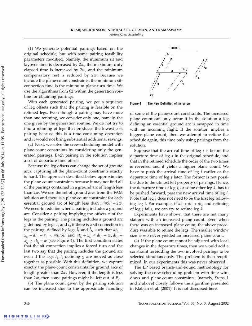
Because the leg offsets can change the set of groundarcs, capturing all the plane-count constraints exactlyis hard. The approach described below approximatesthe plane-count constraints because it may not find allof the pairings contained in a ground arc of length lessthan 2w. We use the set of ground arcs from the FAMsolution and there is a plane-count constraint for eachessential ground arc of length less than minSit+ 2w.We need to redefine when a pairing includes a groundarc. Consider a pairing implying the offsets x of thelegs in the pairing. The pairing includes a ground arcg defined by legs l1 and l2 if there is a sit connection inthe pairing, defined by legs l1 and l2, such that dtl2 +xl2 − atl1 − xl1 < minSit and atl1 + xl1 ≤ dtl1 +w dtl2 +xl2 ≥ atl2 −w (see Figure 4). The first condition statesthat the sit connection implies a forced turn and thelast two say that the pairing includes the ground arceven if the legs l1 l2 defining g are moved as closetogether as possible. With this definition, we captureexactly the plane-count constraints for ground arcs oflength greater than 2w. However, if the length is lessthan 2w, then some pairings might be left out of Pg .

(3) The plane count given by the pairing solutioncan be increased due to the approximate handling

Figure 4 The New Definition of Inclusion

of some of the plane-count constraints. The increasedplane count can only occur if in the solution a legdefining an essential ground arc is swapped in timewith an incoming flight. If the solution implies abigger plane count, then we attempt to retime theschedule again, this time only using pairings from thesolution.

Suppose that the arrival time of leg i is before thedeparture time of leg j in the original schedule, andthat in the retimed schedule the order of the two timesis reversed and it yields a higher plane count. Wehave to push the arrival time of leg i earlier or thedeparture time of leg j later. The former is not possi-ble due to the utmost left property of pairings. Hence,the departure time of leg j, or some other leg k, has tobe pushed forward, past the new arrival time of leg i.Note that leg j does not need to be the first leg follow-ing leg i. For example, if ati < dtj < dtk and retimingof leg j fails, we can try to retime leg k.

Experiments have shown that there are not manystations with an increased plane count. Even whenthere was an increased plane count, the above proce-dure was able to retime the legs. The smaller windowsize w = 5 never yielded an increased plane count.

(4) If the plane count cannot be adjusted with localchanges in the departure times, then we would add aconstraint forbidding the two involved pairings to beselected simultaneously. The problem is then reopti-mized. In our experiments this was never observed.

The LP based branch-and-bound methodology forsolving the crew-scheduling problem with time win-dows and plane-count constraints, (namely, Steps 1and 2 above) closely follows the algorithm presentedin Klabjan et al. (2001). It is not discussed here.


Dow

nloa

ded

from

info

rms.

org

by [

129.

173.

72.8

7] o

n 06

Jul

y 20

14, a

t 11:

05 .

For

pers

onal

use

onl

y, a

ll ri

ghts

res

erve

d.


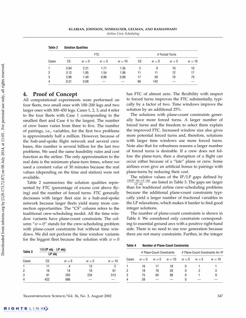
Table 2 Solution Qualities

FTC # Forced Turns

Cases CS w = 0 w = 5 w = 10 CS w = 0 w = 5 w = 10

1 3.94 2.21 1.71 1.35 2 9 10 102 3.12 1.85 1.54 1.06 11 11 12 173 2.86 1.40 0.88 0.88 17 59 70 704 0.31 0.08 — — 66 142 — —

4. Proof of ConceptAll computational experiments were performed onfour fleets, two small ones with 100–200 legs and twolarger ones with 300–450 legs. Cases 1, 2, 3, and 4 referto the four fleets with Case 1 corresponding to thesmallest fleet and Case 4 to the largest. The numberof crew bases varies from three to five. The numberof pairings, i.e., variables, for the first two problemsis approximately half a million. However, because ofthe hub-and-spoke flight network and several crewbases, this number is several billion for the last twoproblems. We used the same feasibility rules and costfunction as the airline. The only approximation to thereal data is the minimum plane-turn times, where weused a constant value of 30 minutes because the realvalues (depending on the time and station) were notavailable.

Table 2 summarizes the solution qualities repre-sented by FTC (percentage of excess cost above fly-ing) and the number of forced turns. FTC generallydecreases with larger fleet size in a hub-and-spokenetwork because larger fleets yield many more con-nection opportunities. The “CS” column refers to thetraditional crew-scheduling model. All the time win-dow variants have plane-count constraints. The col-umn “w = 0” stands for the crew-scheduling problemwith plane-count constraints but without time win-dows. We did not perform the time window variantsfor the biggest fleet because the solution with w = 0

Table 3100�IP obj−LP obj�

LP obj

Cases CS w = 0 w = 5 w = 10

1 11 4 13 32 16 14 10 613 91 203 234 5134 422 686 — —

has FTC of almost zero. The flexibility with respectto forced turns improves the FTC substantially, typi-cally by a factor of two. Time windows improve thesolution by an additional 25%.

The solutions with plane-count constraints gener-ally have more forced turns. A larger number offorced turns and the freedom to select them explainthe improved FTC. Increased window size also givesmore potential forced turns and, therefore, solutionswith larger time windows use more forced turns.Note also that for robustness reasons a larger numberof forced turns is desirable. If a crew does not fol-low the plane-turn, then a disruption of a flight canoccur either because of a “late” plane or crew. Someairlines even give an artificial bonus to pairings withplane-turns by reducing their cost.

The relative values of the IP/LP gaps defined by100�IP obj−LP obj�

LP obj are listed in Table 3. The gaps are largerthan for traditional airline crew-scheduling problemsbecause the additional plane-count constraints typi-cally yield a larger number of fractional variables inthe LP relaxations, which makes it harder to find goodinteger solutions.

The number of plane-count constraints is shown inTable 4. We considered only constraints correspond-ing to essential ground arcs with a positive right-handside. There is no need to use row generation becausethere are not many constraints. Further, in the integer

Table 4 Number of Plane-Count Constraints

# Plane-Count Constraints # Plane-Count Constraints for IP

Cases w = 0 w = 5 w = 10 w = 0 w = 5 w = 10

1 16 17 18 0 1 12 18 19 20 0 2 33 75 84 88 0 1 94 59 — — 0 — —


Dow

nloa

ded

from

info

rms.

org

by [

129.

173.

72.8

7] o

n 06

Jul

y 20

14, a

t 11:

05 .

For

pers

onal

use

onl

y, a

ll ri

ghts

res

erve

d.


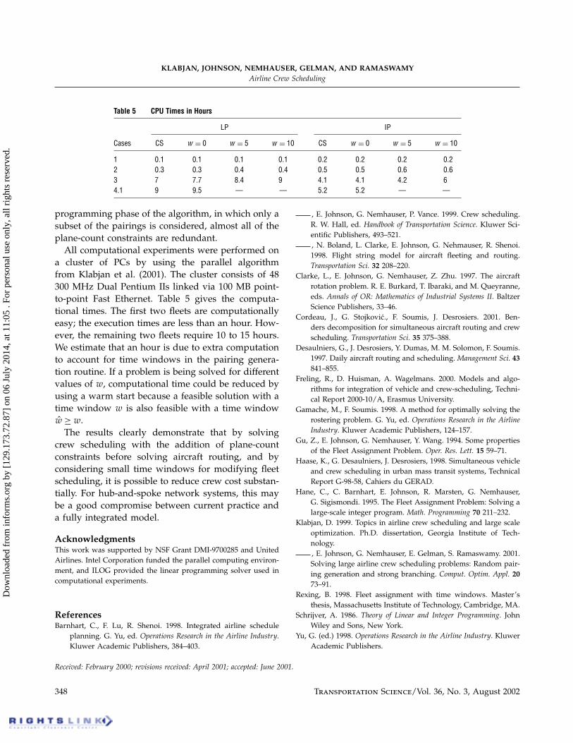
Table 5 CPU Times in Hours

LP IP

Cases CS w = 0 w = 5 w = 10 CS w = 0 w = 5 w = 10

1 0�1 0.1 0.1 0�1 0.2 0.2 0.2 0�22 0�3 0.3 0.4 0�4 0.5 0.5 0.6 0�63 7 7.7 8.4 9 4.1 4.1 4.2 64.1 9 9.5 — — 5.2 5.2 — —

programming phase of the algorithm, in which only asubset of the pairings is considered, almost all of theplane-count constraints are redundant.

All computational experiments were performed ona cluster of PCs by using the parallel algorithmfrom Klabjan et al. (2001). The cluster consists of 48300 MHz Dual Pentium IIs linked via 100 MB point-to-point Fast Ethernet. Table 5 gives the computa-tional times. The first two fleets are computationallyeasy; the execution times are less than an hour. How-ever, the remaining two fleets require 10 to 15 hours.We estimate that an hour is due to extra computationto account for time windows in the pairing genera-tion routine. If a problem is being solved for differentvalues of w, computational time could be reduced byusing a warm start because a feasible solution with atime window w is also feasible with a time windoww ≥w.

The results clearly demonstrate that by solvingcrew scheduling with the addition of plane-countconstraints before solving aircraft routing, and byconsidering small time windows for modifying fleetscheduling, it is possible to reduce crew cost substan-tially. For hub-and-spoke network systems, this maybe a good compromise between current practice anda fully integrated model.

AcknowledgmentsThis work was supported by NSF Grant DMI-9700285 and UnitedAirlines. Intel Corporation funded the parallel computing environ-ment, and ILOG provided the linear programming solver used incomputational experiments.

ReferencesBarnhart, C., F. Lu, R. Shenoi. 1998. Integrated airline schedule

planning. G. Yu, ed. Operations Research in the Airline Industry.Kluwer Academic Publishers, 384–403.

, E. Johnson, G. Nemhauser, P. Vance. 1999. Crew scheduling.R. W. Hall, ed. Handbook of Transportation Science. Kluwer Sci-entific Publishers, 493–521., N. Boland, L. Clarke, E. Johnson, G. Nehmauser, R. Shenoi.1998. Flight string model for aircraft fleeting and routing.Transportation Sci. 32 208–220.

Clarke, L., E. Johnson, G. Nemhauser, Z. Zhu. 1997. The aircraftrotation problem. R. E. Burkard, T. Ibaraki, and M. Queyranne,eds. Annals of OR: Mathematics of Industrial Systems II. BaltzerScience Publishers, 33–46.

Cordeau, J., G. Stojkovic., F. Soumis, J. Desrosiers. 2001. Ben-ders decomposition for simultaneous aircraft routing and crewscheduling. Transportation Sci. 35 375–388.

Desaulniers, G., J. Desrosiers, Y. Dumas, M. M. Solomon, F. Soumis.1997. Daily aircraft routing and scheduling. Management Sci. 43841–855.

Freling, R., D. Huisman, A. Wagelmans. 2000. Models and algo-rithms for integration of vehicle and crew-scheduling, Techni-cal Report 2000-10/A, Erasmus University.

Gamache, M., F. Soumis. 1998. A method for optimally solving therostering problem. G. Yu, ed. Operations Research in the AirlineIndustry. Kluwer Academic Publishers, 124–157.

Gu, Z., E. Johnson, G. Nemhauser, Y. Wang. 1994. Some propertiesof the Fleet Assignment Problem. Oper. Res. Lett. 15 59–71.

Haase, K., G. Desaulniers, J. Desrosiers, 1998. Simultaneous vehicleand crew scheduling in urban mass transit systems, TechnicalReport G-98-58, Cahiers du GERAD.

Hane, C., C. Barnhart, E. Johnson, R. Marsten, G. Nemhauser,G. Sigismondi. 1995. The Fleet Assignment Problem: Solving alarge-scale integer program. Math. Programming 70 211–232.

Klabjan, D. 1999. Topics in airline crew scheduling and large scaleoptimization. Ph.D. dissertation, Georgia Institute of Tech-nology., E. Johnson, G. Nemhauser, E. Gelman, S. Ramaswamy. 2001.Solving large airline crew scheduling problems: Random pair-ing generation and strong branching. Comput. Optim. Appl. 2073–91.

Rexing, B. 1998. Fleet assignment with time windows. Master’sthesis, Massachusetts Institute of Technology, Cambridge, MA.

Schrijver, A. 1986. Theory of Linear and Integer Programming. JohnWiley and Sons, New York.

Yu, G. (ed.) 1998. Operations Research in the Airline Industry. KluwerAcademic Publishers.

Received: February 2000; revisions received: April 2001; accepted: June 2001.


Dow

nloa

ded

from

info

rms.

org

by [

129.

173.

72.8

7] o

n 06

Jul

y 20

14, a

t 11:

05 .

For

pers

onal

use

onl

y, a

ll ri

ghts

res

erve

d.

Documents

Airline Crew Scheduling with Time Windows and Plane-Count Constraints