Page 1 of 22

Analysis of shape and location effects of closely spaced metal loss defects in pressurised pipes

S.S. Al-Owaisi 1, A.A. Becker, W. Sun

Faculty of Engineering, University of Nottingham, Nottingham NG7 2RD, UK

Abstract

Metal loss due to corrosion is a serious threat to the integrity of pressurised oil and gas transmission pipes.

Pipe metal loss defects are found in either single form or in groups (clusters). One of the critical situations

arises when two or more defects are spaced close enough to act as a single lengthier defect with respect to the

axial direction, causing pipe ruptures rather than leaks, and impacting on the pressure containing capacity of a

pipe. There have been few studies conducted to determine the distance needed for defects to interact leading

to a failure pressure lower than that when the defects are treated as single defects and not interacting.

Despite such efforts, there is no universally agreed defect interaction rule and pipe operators around the

world have various rules to pick and choose from. In this work, the effects of defects shape and location on

closely spaced defects are analysed using finite element analysis. The numerical results showed that defect

shapes and locations have a great influence on the peak stress and its location as well as the failure pressure of

pipes containing interacting defects.

Keywords: Interacting defects, Pipe defect assessment, Pipe Integrity

ABBREVIATIONS AN NOMENCLATURE

BC Boundary Condition Circumf. Circumferential Diag. Diagonal E Young’s Modulus Longit. Longitudinal OD Pipe External Diameter PDefect Failure Pressure of Single Defect PMulti Failure Pressure of Interacting Defects S Space Between Defects SMYS Specified Minimum Yield Strength T Pipe Wall Thickness UTS Ultimate Tensile Strength

𝜈 Poisson Ratio

𝜀𝑡𝑟𝑢𝑒 True Strain 𝜀𝑒𝑛𝑔 Engineering Strain

𝜎𝑒𝑛𝑔 Engineering Stress

σEng.UTS

Engineering Ultimate Tensile Strength σeq Defect Equivalent Stress 𝜎𝑡𝑟𝑢𝑒 True Stress σ

TrueUTS True Ultimate Tensile Stress

σY Yield Strength

1 Introduction As pipes age, they get more susceptible to corrosion leading to metal loss both internally and externally. In the

United States alone, there are more than 50% of the gas pipes reaching an age beyond 40 years [1]. Between

1 Corresponding author

Email address: eaxssa@nottingham.ac.uk

Al-Owaisi, SS, Becker, AA, Sun, W, “Analysis of shape and location effects of closely spaced

metal loss defects in pressurised pipes”, S.S. Al-Owaisi, Engineering Failure Analysis, Vol.

68, pp. 172–186 (2016).

Page 2 of 22

2010 and 2013, pipe failures due to corrosion and material degradations resulted in financial loss of more than

$466 million of estimated total costs to gas pipes network operators [1]. Any unplanned shutdown to repair

critical or leaking defects on oil and gas transmission pipes costs millions of dollars which includes costs of

repair and loss of production among others. In 2012 alone, such an unplanned shutdown was carried out to

repair a leaking defect, costing a gas operator $2.9 million to repair a failed pipe and additional 76 million

standard cubic feet of natural gas was released and burned [2].

Metal loss in pipes due to corrosion is a serious threat to the pipe’s structural integrity. Fitness assessment of

metal loss in pipes has been researched since the 1970’s right up to the present time. In chronological order, a

number of examples are given in references [3-17]. Although extensive historical pipeline burst data exist in

the literature, these were done more than 40 years ago on single defects, and data presented are incomplete

due to the fact that earlier defect assessment procedures required only limited information on the defect

geometry (depth and length) and material properties (SMYS and UTS) [18]. One of the critical situations arises

when two or more defects are spaced close enough to interact, i.e. act as a single lengthier defect with respect

to the axial direction, causing major impact on the pressure containing capacity of a pipe [8, 19-21]. Out of all

the available defect assessment recommended practices, DNV-RP-F101 [22] is widely used for the assessment

of interacting defects where previously mentioned literatures show that this recommended practice gives

conservative results in terms of the estimated failure pressure as well as the interaction space between

defects.

While there is a general understanding of the assessment of single metal loss defects, further work remains to

be done to understand the more complex nature of defect interaction. Motivated by the existing work on

metal loss defect interactions, this work addresses a numerical investigation of the effect of defects shape and

location on closely spaced defects using finite element (FE) analysis. The main objective of this study is to

conduct a systematic parametric evaluation of the location and shape effects in API5L X60. The outcome of

this work is to develop simplified criteria on defect interaction rules aimed towards reducing conservatism to

assess the consequences of failure and determining the pressure containing capacity of pipe, thus impacting

directly on unplanned shutdowns, and the number of repairs to maintain the integrity of the pipes within the

envelope of health, safety and environment (HSE).

2 Nonlinear Finite Element Analysis (FEA) Parametric investigations of the effect of shape and location of closely spaced defects were carried out using

the Abaqus 6.14 FEA software [23]. Artificial corrosion defects with the same length and width were used in

the models. The length to width ratio was kept the same (35 mm each) for all defects. The defect depth was

constant for all defects, as 50% of the wall thickness. However, further modifications of the defect depth and

spacing between defects were made to investigate the effects of interaction. For the sake of practicality and

to represent real-life defects, the dimensions were chosen to be in line with the pipeline operator forum (POF)

[24] for general corrosion, and as such these defect types can be detected and sized, and interaction roles can

easily be applied by the existing pipe inspection tools. Additionally, such general corrosion defects are widely

observed in service in the oil and gas pipes industry.

Page 3 of 22

2.1 Material properties

Ductile carbon steel is used in this study as it is a commonly used material in the oil and gas pipes. The pipe

material properties were based on existing literature, giving the true stress and plastic strain data for the X80

[20] and X60 [25] pipes. The material is modelled as an isotropic elasto-plastic material and true stress-true

strain data are employed within Abaqus. It is acknowledged that some anisotropic behaviour does exist in the

pipes as a result of the manufacturing processes; however, considering that the isotropic behaviour has

yielded accurate results in terms of predicting failure pressure as reported by many researchers in the past [8,

11, 15, 16, 26-28], only an isotropic hardening rule is used in this work. The true stress-strain values are

obtained from the engineering uniaxial stress-stress data using equations (1) and (2) which are only valid up to

necking where the loading situation is no longer uniaxial throughout the gauge length [29]:

𝜀𝑡𝑟𝑢𝑒 = ln(1 + 𝜀𝑒𝑛𝑔)

(1)

𝜎𝑡𝑟𝑢𝑒 = 𝜎𝑒𝑛𝑔(1 + 𝜀𝑒𝑛𝑔)

(2)

where eng and eng are the engineering (nominal) stress and strain respectively, while true and true are the

true stress and strain respectively. Both material nonlinearity and nonlinear geometry (NLGEOM parameter in

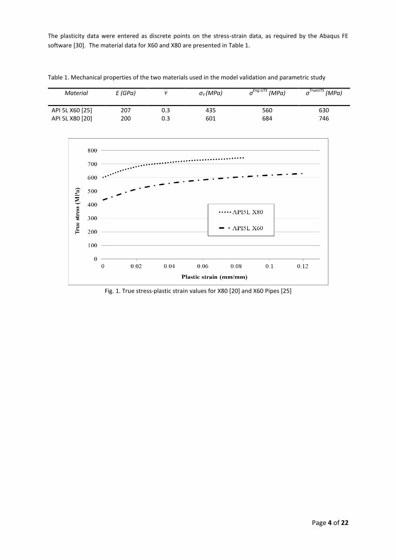
Abaqus) were invoked in the analysis. The stress-strain curves used in this study are presented in Fig. 1. Fig. 1.

True stress-plastic strain values for X80 [20] and X60 Pipes [25]

Page 4 of 22

The plasticity data were entered as discrete points on the stress-strain data, as required by the Abaqus FE

software [30]. The material data for X60 and X80 are presented in Table 1.

Table 1. Mechanical properties of the two materials used in the model validation and parametric study

Material E (GPa) 𝜈 σY (MPa) σEng.UTS

(MPa) σTrueUTS

(MPa)

API 5L X60 [25] 207 0.3 435 560 630 API 5L X80 [20] 200 0.3 601 684 746

Fig. 1. True stress-plastic strain values for X80 [20] and X60 Pipes [25]

Page 5 of 22

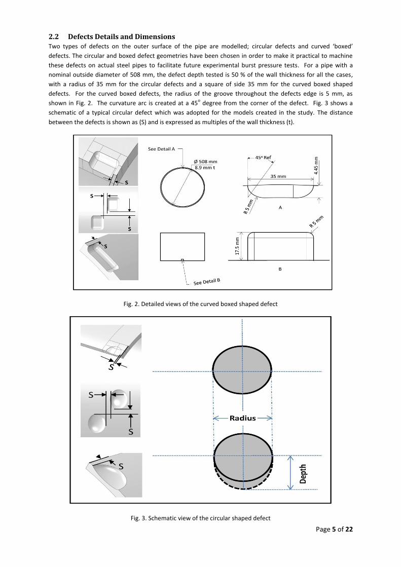
2.2 Defects Details and Dimensions Two types of defects on the outer surface of the pipe are modelled; circular defects and curved ‘boxed’

defects. The circular and boxed defect geometries have been chosen in order to make it practical to machine

these defects on actual steel pipes to facilitate future experimental burst pressure tests. For a pipe with a

nominal outside diameter of 508 mm, the defect depth tested is 50 % of the wall thickness for all the cases,

with a radius of 35 mm for the circular defects and a square of side 35 mm for the curved boxed shaped

defects. For the curved boxed defects, the radius of the groove throughout the defects edge is 5 mm, as

shown in Fig. 2. The curvature arc is created at a 45o degree from the corner of the defect. Fig. 3 shows a

schematic of a typical circular defect which was adopted for the models created in the study. The distance

between the defects is shown as (S) and is expressed as multiples of the wall thickness (t).

Fig. 2. Detailed views of the curved boxed shaped defect

Fig. 3. Schematic view of the circular shaped defect

Page 6 of 22

2.3 Problem Definition As indicated in Section 2.1, the pipe materials used in this work were composed of pipes made of API 5L X60

and X80 steel. Both of the materials were initially used to compare the present FE solutions to other published

FE solutions, and later X60 was used for the parametric study. Pipes are normally manufactured in average

lengths of 12 meters. However, the numerical simulation study uses pipe lengths of 1.8 m which has been

demonstrated in the literature to be sufficient to cater for the end effects [25, 31]. The 1.8 m pipe length is

chosen here as a practical pipe length to enable future experimental laboratory tests of pipe burst pressures.

The nominal outside diameter is 508 mm with wall thicknesses of 8.9 mm for X60 while X80 nominal outside

diameter is 458.8 with a wall thickness of 8.1 mm.

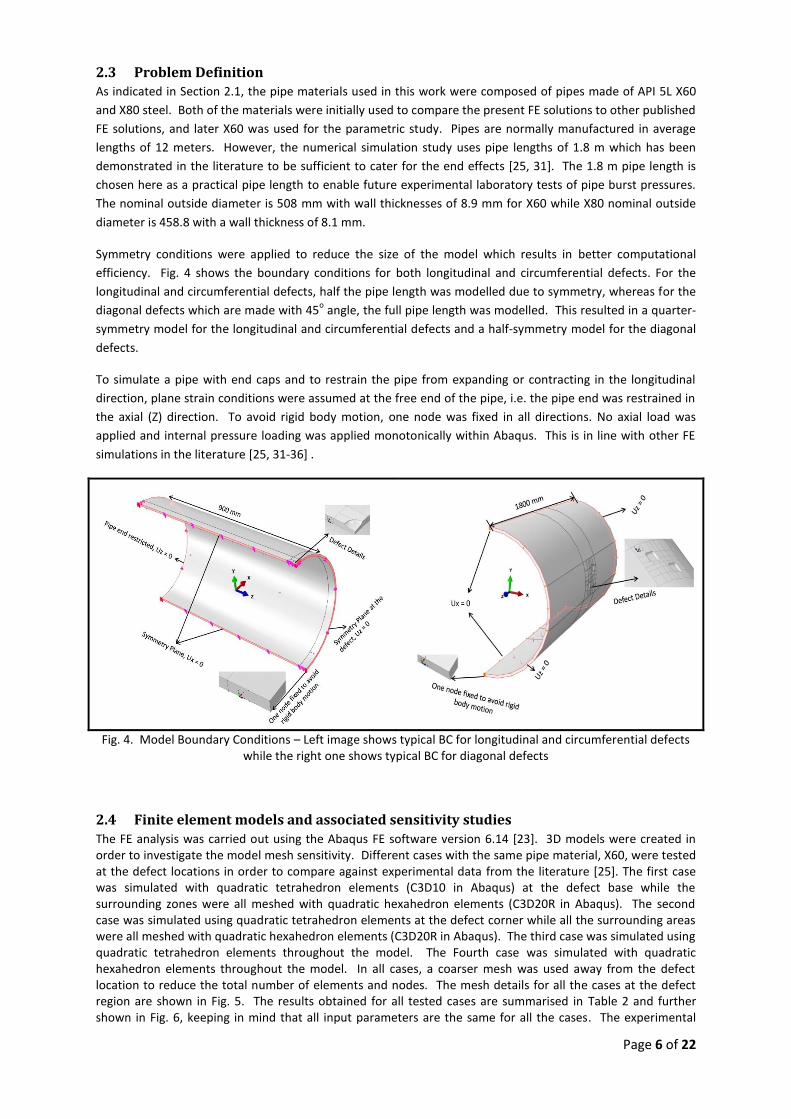
Symmetry conditions were applied to reduce the size of the model which results in better computational

efficiency. Fig. 4 shows the boundary conditions for both longitudinal and circumferential defects. For the

longitudinal and circumferential defects, half the pipe length was modelled due to symmetry, whereas for the

diagonal defects which are made with 45o angle, the full pipe length was modelled. This resulted in a quarter-

symmetry model for the longitudinal and circumferential defects and a half-symmetry model for the diagonal

defects.

To simulate a pipe with end caps and to restrain the pipe from expanding or contracting in the longitudinal

direction, plane strain conditions were assumed at the free end of the pipe, i.e. the pipe end was restrained in

the axial (Z) direction. To avoid rigid body motion, one node was fixed in all directions. No axial load was

applied and internal pressure loading was applied monotonically within Abaqus. This is in line with other FE

simulations in the literature [25, 31-36] .

Fig. 4. Model Boundary Conditions – Left image shows typical BC for longitudinal and circumferential defects while the right one shows typical BC for diagonal defects

2.4 Finite element models and associated sensitivity studies

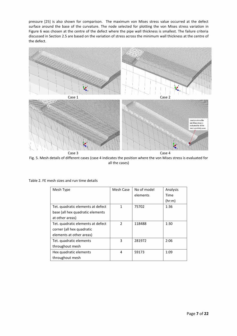
The FE analysis was carried out using the Abaqus FE software version 6.14 [23]. 3D models were created in order to investigate the model mesh sensitivity. Different cases with the same pipe material, X60, were tested at the defect locations in order to compare against experimental data from the literature [25]. The first case was simulated with quadratic tetrahedron elements (C3D10 in Abaqus) at the defect base while the surrounding zones were all meshed with quadratic hexahedron elements (C3D20R in Abaqus). The second case was simulated using quadratic tetrahedron elements at the defect corner while all the surrounding areas were all meshed with quadratic hexahedron elements (C3D20R in Abaqus). The third case was simulated using quadratic tetrahedron elements throughout the model. The Fourth case was simulated with quadratic hexahedron elements throughout the model. In all cases, a coarser mesh was used away from the defect location to reduce the total number of elements and nodes. The mesh details for all the cases at the defect region are shown in Fig. 5. The results obtained for all tested cases are summarised in Table 2 and further shown in Fig. 6, keeping in mind that all input parameters are the same for all the cases. The experimental

Page 7 of 22

pressure [25] is also shown for comparison. The maximum von Mises stress value occurred at the defect surface around the base of the curvature. The node selected for plotting the von Mises stress variation in Figure 6 was chosen at the centre of the defect where the pipe wall thickness is smallest. The failure criteria discussed in Section 2.5 are based on the variation of stress across the minimum wall thickness at the centre of the defect.

Case 1

Case 2

Case 3

Case 4

Fig. 5. Mesh details of different cases (case 4 indicates the position where the von Mises stress is evaluated for all the cases)

Table 2. FE mesh sizes and run time details

Mesh Type Mesh Case No of model

elements

Analysis

Time

(hr:m)

Tet. quadratic elements at defect

base (all hex quadratic elements

at other areas)

1 75702

1:36

Tet. quadratic elements at defect

corner (all hex quadratic

elements at other areas)

2 118488 1:30

Tet. quadratic elements

throughout mesh

3 281972 2:06

Hex quadratic elements

throughout mesh

4 59173 1:09

Page 8 of 22

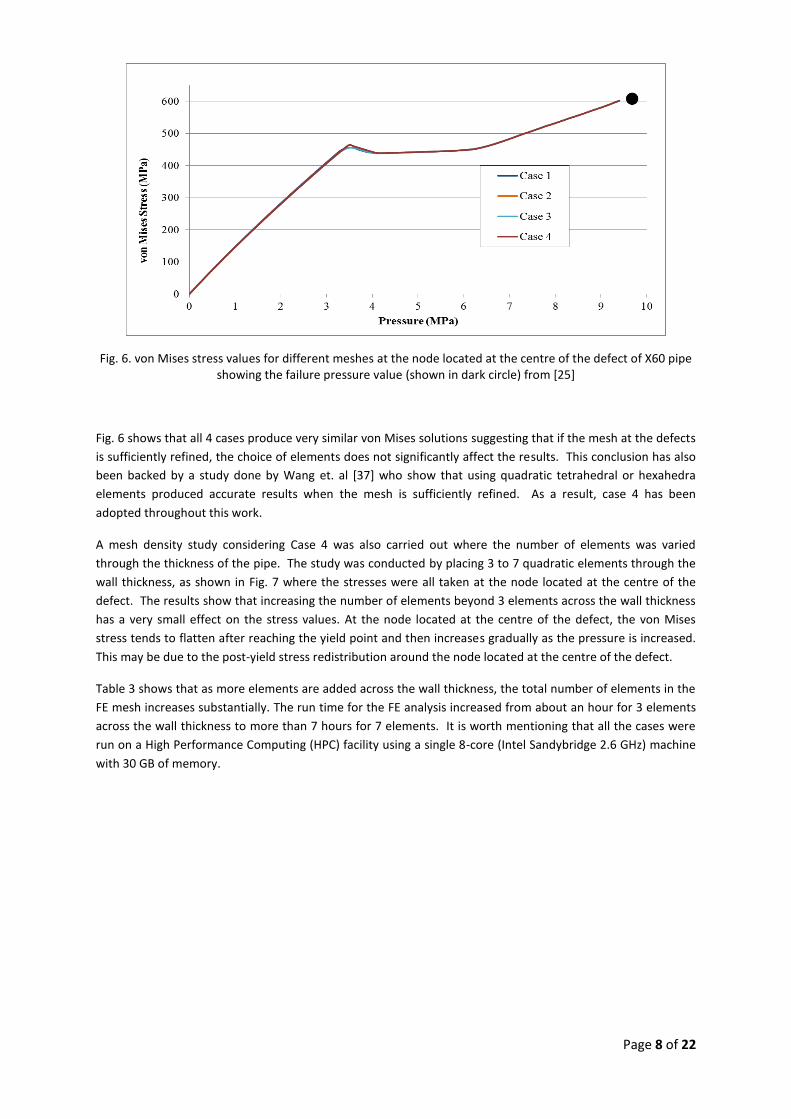
Fig. 6. von Mises stress values for different meshes at the node located at the centre of the defect of X60 pipe showing the failure pressure value (shown in dark circle) from [25]

Fig. 6 shows that all 4 cases produce very similar von Mises solutions suggesting that if the mesh at the defects

is sufficiently refined, the choice of elements does not significantly affect the results. This conclusion has also

been backed by a study done by Wang et. al [37] who show that using quadratic tetrahedral or hexahedra

elements produced accurate results when the mesh is sufficiently refined. As a result, case 4 has been

adopted throughout this work.

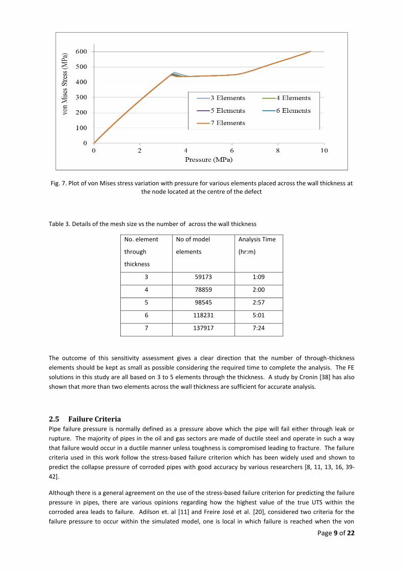
A mesh density study considering Case 4 was also carried out where the number of elements was varied

through the thickness of the pipe. The study was conducted by placing 3 to 7 quadratic elements through the

wall thickness, as shown in Fig. 7 where the stresses were all taken at the node located at the centre of the

defect. The results show that increasing the number of elements beyond 3 elements across the wall thickness

has a very small effect on the stress values. At the node located at the centre of the defect, the von Mises

stress tends to flatten after reaching the yield point and then increases gradually as the pressure is increased.

This may be due to the post-yield stress redistribution around the node located at the centre of the defect.

Table 3 shows that as more elements are added across the wall thickness, the total number of elements in the

FE mesh increases substantially. The run time for the FE analysis increased from about an hour for 3 elements

across the wall thickness to more than 7 hours for 7 elements. It is worth mentioning that all the cases were

run on a High Performance Computing (HPC) facility using a single 8-core (Intel Sandybridge 2.6 GHz) machine

with 30 GB of memory.

Page 9 of 22

Fig. 7. Plot of von Mises stress variation with pressure for various elements placed across the wall thickness at the node located at the centre of the defect

Table 3. Details of the mesh size vs the number of across the wall thickness

No. element

through

thickness

No of model

elements

Analysis Time

(hr:m)

3 59173 1:09

4 78859 2:00

5 98545 2:57

6 118231 5:01

7 137917 7:24

The outcome of this sensitivity assessment gives a clear direction that the number of through-thickness

elements should be kept as small as possible considering the required time to complete the analysis. The FE

solutions in this study are all based on 3 to 5 elements through the thickness. A study by Cronin [38] has also

shown that more than two elements across the wall thickness are sufficient for accurate analysis.

2.5 Failure Criteria

Pipe failure pressure is normally defined as a pressure above which the pipe will fail either through leak or

rupture. The majority of pipes in the oil and gas sectors are made of ductile steel and operate in such a way

that failure would occur in a ductile manner unless toughness is compromised leading to fracture. The failure

criteria used in this work follow the stress-based failure criterion which has been widely used and shown to

predict the collapse pressure of corroded pipes with good accuracy by various researchers [8, 11, 13, 16, 39-

42].

Although there is a general agreement on the use of the stress-based failure criterion for predicting the failure

pressure in pipes, there are various opinions regarding how the highest value of the true UTS within the

corroded area leads to failure. Adilson et. al [11] and Freire José et al. [20], considered two criteria for the

failure pressure to occur within the simulated model, one is local in which failure is reached when the von

Page 10 of 22

Mises stress at any point of the defect region attains the true UTS of the material, while the second one which

is global considers failure to take place when the nonlinear analysis algorithm in the FE software does not

attain convergence. Filho et. al [16] used a similar failure criterion as suggested by Adilson et. al [11] where

the pipe is considered to have failed when any element reaches stresses equal to the material’s true UTS

value. Bedairi et. al [25] stated that failure pressure within the FE model was reached when the von Mises

stress at the defect bottom reaches the true UTS of the material. Ma Bin et. al [34] considered failure to take

place once the von Mises equivalent stress at the mid surface of the corroded ligament reaches the true UTS of

the material. Fekte et. al [27] considered the failure pressure of the corroded pipes to occur when the von

Mises equivalent stress at the deepest point of the defect area reaches the true UTS of the considered pipe

material.

The choice of using a stress-based failure criterion also follows the pipe design codes such as ASME B31.4

[43]and ASME B31.8 [44] which are based mainly on stress-based designs considering various assumptions

such as plane stress using isotropic, linear elastic and homogeneous materials where displacements are very

small. The strain-based approach which postulates that failure occurs when the applied strain exceeds the

maximum strain value during burst was refuted by Chouchaoui [8] as it reveals large scatters in the prediction

of the pipe failure pressure. Additionally, failure of the local wall-thinned pipe under internal pressure is a

failure by load-controlled loading rather than displacement-controlled loading [13]. The stress-based failure

criterion, which is based on the von Mises criterion, suggests that failure is initiated when the stress at the

metal loss site reaches the pipe material’s true UTS. The stress-based failure criterion is used below to predict

yielding of the pipe material based on results obtained from the uniaxial tensile test data.

Failure criteria that are based on the von Mises stress at a single point (node) reaching the true UTS of the

material in the defect zone, would be highly sensitive to the degree of mesh refinement around the defect

region. Failure criteria based on the von Mises stresses at all points across the thickness of the pipe at the

defect region are less sensitive to mesh refinement. Therefore, two failure criteria are adopted in this work.

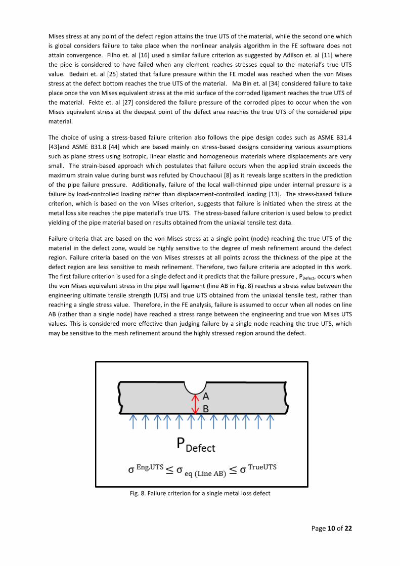
The first failure criterion is used for a single defect and it predicts that the failure pressure , PDefect, occurs when

the von Mises equivalent stress in the pipe wall ligament (line AB in Fig. 8) reaches a stress value between the

engineering ultimate tensile strength (UTS) and true UTS obtained from the uniaxial tensile test, rather than

reaching a single stress value. Therefore, in the FE analysis, failure is assumed to occur when all nodes on line

AB (rather than a single node) have reached a stress range between the engineering and true von Mises UTS

values. This is considered more effective than judging failure by a single node reaching the true UTS, which

may be sensitive to the mesh refinement around the highly stressed region around the defect.

Fig. 8. Failure criterion for a single metal loss defect

Page 11 of 22

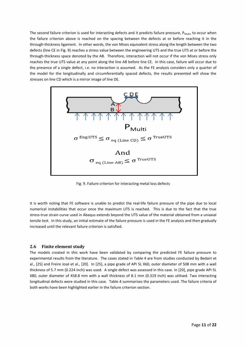
The second failure criterion is used for interacting defects and it predicts failure pressure, PMulti, to occur when

the failure criterion above is reached on the spacing between the defects at or before reaching it in the

through-thickness ligament. In other words, the von Mises equivalent stress along the length between the two

defects (line CE in Fig. 9) reaches a stress value between the engineering UTS and the true UTS at or before the

through-thickness space denoted by the AB. Therefore, interaction will not occur if the von Mises stress only

reaches the true UTS value at any point along the line AB before line CE. In this case, failure will occur due to

the presence of a single defect, i.e. no interaction is assumed. As the FE analysis considers only a quarter of

the model for the longitudinally and circumferentially spaced defects, the results presented will show the

stresses on line CD which is a mirror image of line DE.

Fig. 9. Failure criterion for interacting metal loss defects

It is worth noting that FE software is unable to predict the real-life failure pressure of the pipe due to local

numerical instabilities that occur once the maximum UTS is reached. This is due to the fact that the true

stress-true strain curve used in Abaqus extends beyond the UTS value of the material obtained from a uniaxial

tensile test. In this study, an initial estimate of the failure pressure is used in the FE analysis and then gradually

increased until the relevant failure criterion is satisfied.

2.6 Finite element study

The models created in this work have been validated by comparing the predicted FE failure pressure to

experimental results from the literature. The cases stated in Table 4 are from studies conducted by Bedairi et

al., [25] and Freire José et al., [20]. In [25], a pipe grade of API 5L X60, outer diameter of 508 mm with a wall

thickness of 5.7 mm (0.224 inch) was used. A single defect was assessed in this case. In [20], pipe grade API 5L

X80, outer diameter of 458.8 mm with a wall thickness of 8.1 mm (0.319 inch) was utilised. Two interacting

longitudinal defects were studied in this case. Table 4 summarises the parameters used. The failure criteria of

both works have been highlighted earlier in the failure criterion section.

Page 12 of 22

Table 4: Model validation results

No Ref. Pipe Defects Details Published Experimental

Burst Pressure

(MPa)

Published FEA Failure

Pressure (MPa)

FEA Failure Value in this work (MPa)

Percentage difference

Published Experimental

Burst pressure

Published FEA Failure

Pressure

1

Bedairi et al.,

[25]

X60 OD: 508 mm

t: 5.7 mm Defect type: Rectangular Defect Length: 200 mm Defect Width: 30 mm

Defect depth: 45%

9.59 9.42 9.4 2% 0.2%

2 Freire

José, et al., [20]

X80 OD: 458.8 mm

t: 8.1 mm Defect type: Rectangular Defect Length: 39.6 mm Defect Width: 31.9 mm

Defect depth: 5.32 Spacing: 20.5 mm

20.30 19.60 19.33 5% 2%

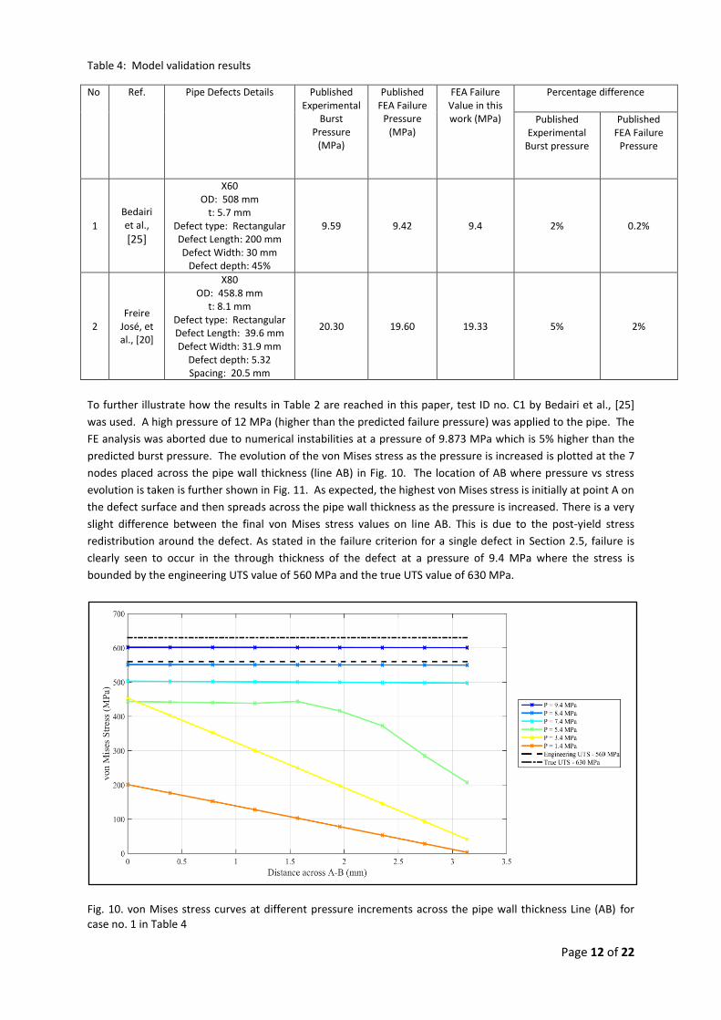
To further illustrate how the results in Table 2 are reached in this paper, test ID no. C1 by Bedairi et al., [25]

was used. A high pressure of 12 MPa (higher than the predicted failure pressure) was applied to the pipe. The

FE analysis was aborted due to numerical instabilities at a pressure of 9.873 MPa which is 5% higher than the

predicted burst pressure. The evolution of the von Mises stress as the pressure is increased is plotted at the 7

nodes placed across the pipe wall thickness (line AB) in Fig. 10. The location of AB where pressure vs stress

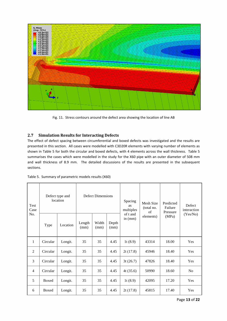
evolution is taken is further shown in Fig. 11. As expected, the highest von Mises stress is initially at point A on

the defect surface and then spreads across the pipe wall thickness as the pressure is increased. There is a very

slight difference between the final von Mises stress values on line AB. This is due to the post-yield stress

redistribution around the defect. As stated in the failure criterion for a single defect in Section 2.5, failure is

clearly seen to occur in the through thickness of the defect at a pressure of 9.4 MPa where the stress is

bounded by the engineering UTS value of 560 MPa and the true UTS value of 630 MPa.

Fig. 10. von Mises stress curves at different pressure increments across the pipe wall thickness Line (AB) for case no. 1 in Table 4

Page 13 of 22

Fig. 11. Stress contours around the defect area showing the location of line AB

2.7 Simulation Results for Interacting Defects The effect of defect spacing between circumferential and boxed defects was investigated and the results are

presented in this section. All cases were modelled with C3D20R elements with varying number of elements as

shown in Table 5 for both the circular and boxed defects, with 4 elements across the wall thickness. Table 5

summarises the cases which were modelled in the study for the X60 pipe with an outer diameter of 508 mm

and wall thickness of 8.9 mm. The detailed discussions of the results are presented in the subsequent

sections.

Table 5. Summary of parametric models results (X60)

Test

Case

No.

Defect type and

location

Defect Dimensions

Spacing

as

multiples

of t and

in (mm)

Mesh Size

(total no.

of

elements)

Predicted

Failure

Pressure

(MPa)

Defect

interaction

(Yes/No)

Type Location Length

(mm)

Width

(mm)

Depth

(mm)

1 Circular Longit. 35 35 4.45 1t (8.9) 43314 18.00 Yes

2 Circular Longit. 35 35 4.45 2t (17.8) 45946 18.40 Yes

3 Circular Longit. 35 35 4.45 3t (26.7) 47826 18.40 Yes

4 Circular Longit. 35 35 4.45 4t (35.6) 50990 18.60 No

5 Boxed Longit. 35 35 4.45 1t (8.9) 42095 17.20 Yes

6 Boxed Longit. 35 35 4.45 2t (17.8) 45815 17.40 Yes

Page 14 of 22

7 Boxed

Longit. 35 35 4.45 3t (26.7) 48791 17.60 Yes

8 Boxed

Longit. 35 35 4.45 4t (35.6) 52511 17.60 No

9 Circular Circumf. 35 35 7.12 1t (8.9) 42652 16.80 No

10 Circular Circumf. 35 35 4.45 0.5t

(4.45) 42486 19.40 No

11 Boxed

Circumf. 35 35 7.12 1t (8.9) 47150 15.00 No

12 Boxed

Circumf. 35 35 4.45 0.5t

(4.45) 44984 18.88 No

13 Circular Diag. 35 35 4.45 1t (8.9) 191752 18.90 No

14 Circular Diag. 35 35 4.45 0.5t

(4.45) 189256 18.90 No

15 Boxed

Diag. 35 35 4.45 1t (8.9) 157660 17.60 No

16 Boxed

Diag. 35 35 4.45 0.5t

(4.45) 154780 17.40 Yes

2.7.1 Effect of spacing on circular defects

2.7.1.1 Spacing in the longitudinal direction

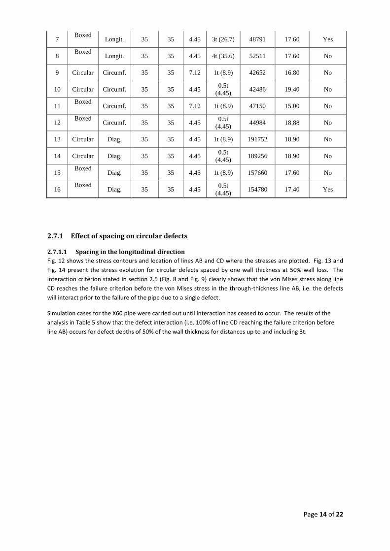
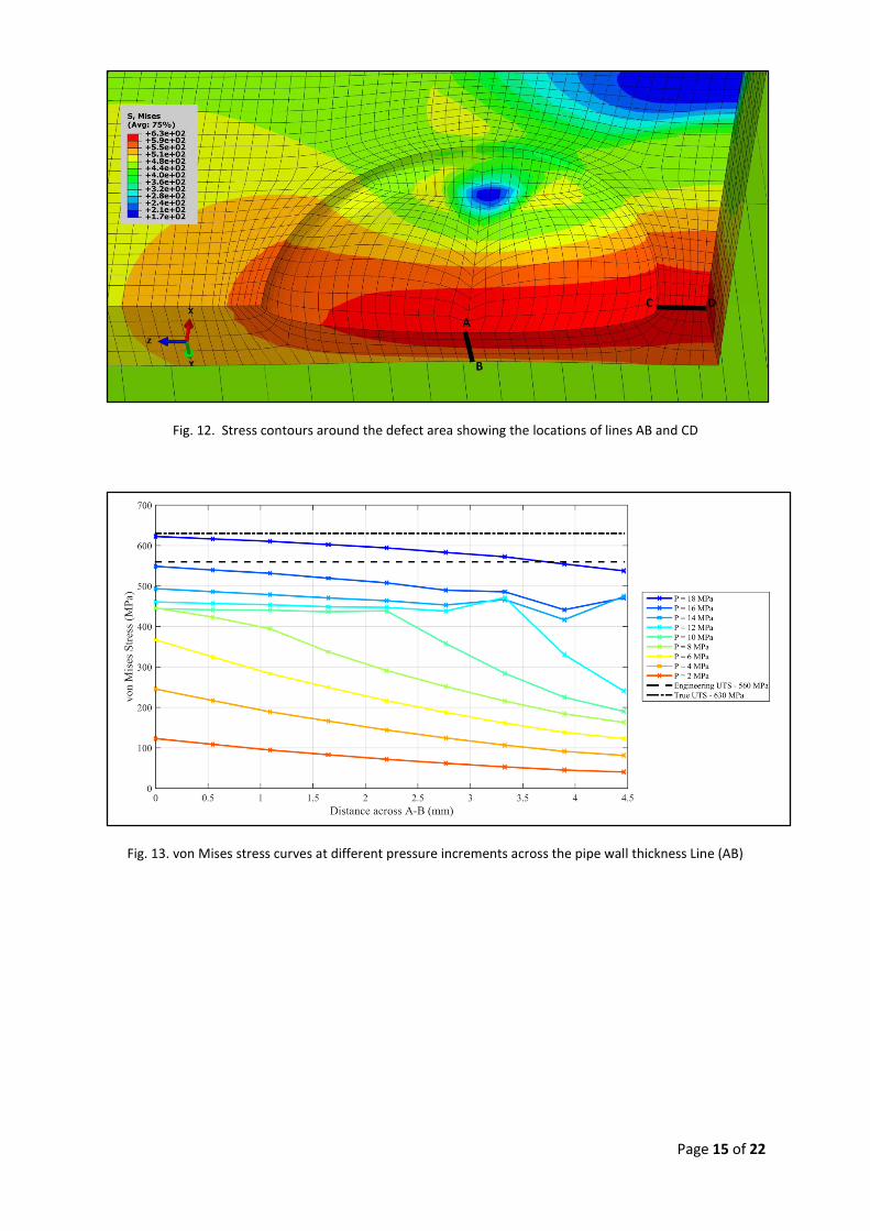
Fig. 12 shows the stress contours and location of lines AB and CD where the stresses are plotted. Fig. 13 and

Fig. 14 present the stress evolution for circular defects spaced by one wall thickness at 50% wall loss. The

interaction criterion stated in section 2.5 (Fig. 8 and Fig. 9) clearly shows that the von Mises stress along line

CD reaches the failure criterion before the von Mises stress in the through-thickness line AB, i.e. the defects

will interact prior to the failure of the pipe due to a single defect.

Simulation cases for the X60 pipe were carried out until interaction has ceased to occur. The results of the

analysis in Table 5 show that the defect interaction (i.e. 100% of line CD reaching the failure criterion before

line AB) occurs for defect depths of 50% of the wall thickness for distances up to and including 3t.

Page 15 of 22

Fig. 12. Stress contours around the defect area showing the locations of lines AB and CD

Fig. 13. von Mises stress curves at different pressure increments across the pipe wall thickness Line (AB)

Page 16 of 22

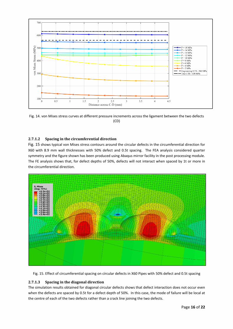
Fig. 14. von Mises stress curves at different pressure increments across the ligament between the two defects (CD)

2.7.1.2 Spacing in the circumferential direction

Fig. 15 shows typical von Mises stress contours around the circular defects in the circumferential direction for

X60 with 8.9 mm wall thicknesses with 50% defect and 0.5t spacing. The FEA analysis considered quarter

symmetry and the figure shown has been produced using Abaqus mirror facility in the post processing module.

The FE analysis shows that, for defect depths of 50%, defects will not interact when spaced by 1t or more in

the circumferential direction.

Fig. 15. Effect of circumferential spacing on circular defects in X60 Pipes with 50% defect and 0.5t spacing

2.7.1.3 Spacing in the diagonal direction

The simulation results obtained for diagonal circular defects shows that defect interaction does not occur even

when the defects are spaced by 0.5t for a defect depth of 50%. In this case, the mode of failure will be local at

the centre of each of the two defects rather than a crack line joining the two defects.

Page 17 of 22

2.7.2 Effect of Spacing on boxed shape defects

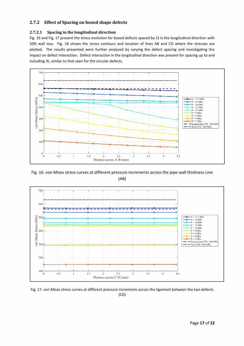
2.7.2.1 Spacing in the longitudinal direction

Fig. 16 and Fig. 17 present the stress evolution for boxed defects spaced by 1t in the longitudinal direction with

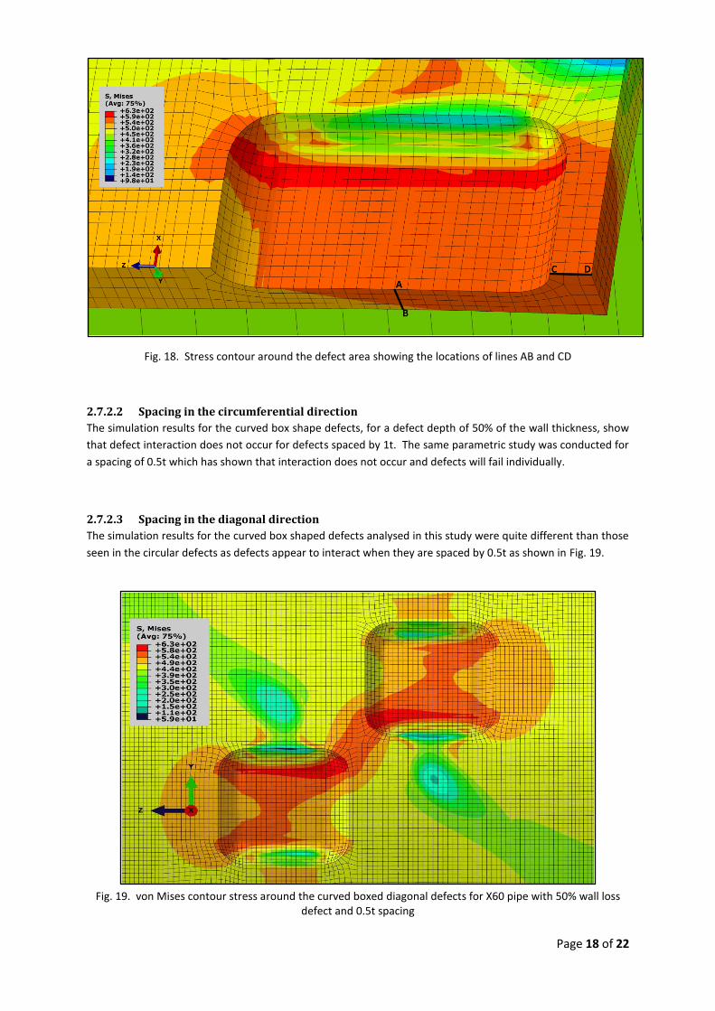
50% wall loss. Fig. 18 shows the stress contours and location of lines AB and CD where the stresses are

plotted. The results presented were further analysed by varying the defect spacing and investigating the

impact on defect interaction. Defect interaction in the longitudinal direction was present for spacing up to and

including 3t, similar to that seen for the circular defects.

Fig. 16. von Mises stress curves at different pressure increments across the pipe wall thickness Line

(AB)

Fig. 17. von Mises stress curves at different pressure increments across the ligament between the two defects (CD)

Page 18 of 22

Fig. 18. Stress contour around the defect area showing the locations of lines AB and CD

2.7.2.2 Spacing in the circumferential direction

The simulation results for the curved box shape defects, for a defect depth of 50% of the wall thickness, show

that defect interaction does not occur for defects spaced by 1t. The same parametric study was conducted for

a spacing of 0.5t which has shown that interaction does not occur and defects will fail individually.

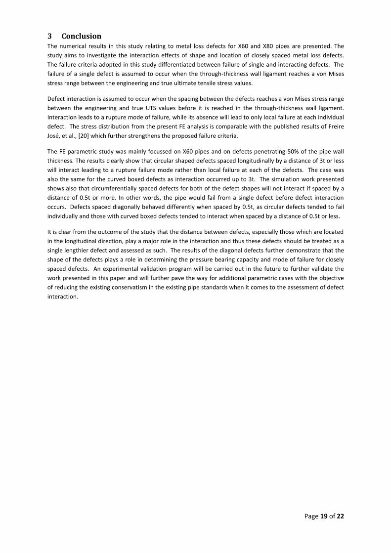
2.7.2.3 Spacing in the diagonal direction

The simulation results for the curved box shaped defects analysed in this study were quite different than those

seen in the circular defects as defects appear to interact when they are spaced by 0.5t as shown in Fig. 19.

Fig. 19. von Mises contour stress around the curved boxed diagonal defects for X60 pipe with 50% wall loss

defect and 0.5t spacing

Page 19 of 22

3 Conclusion The numerical results in this study relating to metal loss defects for X60 and X80 pipes are presented. The

study aims to investigate the interaction effects of shape and location of closely spaced metal loss defects.

The failure criteria adopted in this study differentiated between failure of single and interacting defects. The

failure of a single defect is assumed to occur when the through-thickness wall ligament reaches a von Mises

stress range between the engineering and true ultimate tensile stress values.

Defect interaction is assumed to occur when the spacing between the defects reaches a von Mises stress range

between the engineering and true UTS values before it is reached in the through-thickness wall ligament.

Interaction leads to a rupture mode of failure, while its absence will lead to only local failure at each individual

defect. The stress distribution from the present FE analysis is comparable with the published results of Freire

José, et al., [20] which further strengthens the proposed failure criteria.

The FE parametric study was mainly focussed on X60 pipes and on defects penetrating 50% of the pipe wall

thickness. The results clearly show that circular shaped defects spaced longitudinally by a distance of 3t or less

will interact leading to a rupture failure mode rather than local failure at each of the defects. The case was

also the same for the curved boxed defects as interaction occurred up to 3t. The simulation work presented

shows also that circumferentially spaced defects for both of the defect shapes will not interact if spaced by a

distance of 0.5t or more. In other words, the pipe would fail from a single defect before defect interaction

occurs. Defects spaced diagonally behaved differently when spaced by 0.5t, as circular defects tended to fail

individually and those with curved boxed defects tended to interact when spaced by a distance of 0.5t or less.

It is clear from the outcome of the study that the distance between defects, especially those which are located

in the longitudinal direction, play a major role in the interaction and thus these defects should be treated as a

single lengthier defect and assessed as such. The results of the diagonal defects further demonstrate that the

shape of the defects plays a role in determining the pressure bearing capacity and mode of failure for closely

spaced defects. An experimental validation program will be carried out in the future to further validate the

work presented in this paper and will further pave the way for additional parametric cases with the objective

of reducing the existing conservatism in the existing pipe standards when it comes to the assessment of defect

interaction.

Page 20 of 22

References

1. NTSB, Integrity Management of Gas Transmission Pipelines in High Consequence Areas. 2015, National Transportation Safety Board: Washingon, DC, USA.

2. NTSB, Columbia Gas Transmission Corporation Pipeline Rupture. 2014, National Transportation Safety Board: Washington DC, USA.

3. Kiefner, J.F., Maxey, W.A., Eiber, R.J. and Duffy, A.R., Failure Stress Levels of Flaws in Pressurized Cylinders. 1973, ASTM: USA. p. 461-481.

4. Shannon, R.W.E., The failure behaviour of line pipe defects. International Journal of Pressure Vessels and Piping, 1974. 2(4): p. 243-255.

5. Kiefner, J. and Vieth, P., New method corrects criterion for evaluating corroded pipe. Oil and Gas Journal, 1990. 8.

6. ASME, A.S.o.M.E., Manual for Determining the Remaining Strength of Corroded Pipelines. 1984, ASME: USA.

7. Kirkwood, M., Fu, B., Vu, D. and Batte, A. Assessing the Integrity of Corroded Linepipe-An Industry Initiative. in Aspect'96: Advances in Subsea Pipeline Engineering and Technology. 1996. Society of Underwater Technology.

8. Chouchaoui, B.A. and Pick, R.J., Behaviour of longitudinally aligned corrosion pits. International Journal of Pressure Vessels and Piping, 1996. 67(1): p. 18.

9. Bjornoy, O.H., Sigurdsson, G. and Marley, M.J. Background and Development of DNV-RP-F101 "Corroded Pipelines". in Proceedings of the Eleventh (2001) International Offshore and Polar Engineering Conference. 2001. Stavanger, Norway.

10. Cosham, A. and Hopkins, P. Pipeline Defect Assessment Manual PDAM. in International Pipeline Conference. 2002. Calgary, Alberta, Canada.

11. Benjamin, A.C. and Andrade, E.Q.d. Predicting the failure pressure of pipelines containing nonuniform depth of corrosion defects using FEA. in Proceedings of OMAE’03: 22nd International Conference on Offshore Mechanics and Arctic Engineering. 2003. Cancun, Mexico.

12. Netto, T.A., Ferraz, U.S. and Botto, A., On the effect of corrosion defects on the collapse pressure of pipelines. International Journal of Solids and Structures, 2007. 44(22-23): p. 7597-7614.

13. Kim, J.W., Park, C.Y. and Lee, S.H., Local Failure Criteria for Wall-Thinning Defect in Piping Components based on Simulated Specimen and Real-Scale Pipe Tests, in 20th International Conference on Structural Mechanics in Reactor Technology (SMiRT 20) 2009: Espoo, Finland.

14. Belachew, C.T., Ismail, M.C. and Karuppanan, S., Burst Strength Analysis of Corroded Pipelines by Finite Element Method. J. Applied Sci., 2011. 11: p. 1845-1850.

15. Hosseini, A., Cronin, D.S. and Plumtree, A., Crack in Corrosion Defect Assessment in Transmission Pipelines. Journal of Pressure Vessel Technology, 2013. 135: p. 8.

Page 21 of 22

16. Abdalla Filho, J.E., Machado, R.D., Bertin, R.J. and Valentini, M.D., On the failure pressure of pipelines containing wall reduction and isolated pit corrosion defects. Computers & Structures, 2014. 132(0): p. 22-33.

17. Yeom, K.J., Lee, Y.-K., Oh, K.H. and Kim, W.S., Integrity assessment of a corroded API X70 pipe with a single defect by burst pressure analysis. Engineering Failure Analysis, 2015. 57: p. 553-561.

18. Cronin, D.S. and Pick, R.J. Experimental Database for Corroded Pipe: Evaluation of RSTRENG and B31G. in PROCEEDINGS OF THE INTERNATIONAL PIPELINE CONFERENCE. 2000.

19. Cronin, D.S. and Pick, R.J., Prediction of the failure pressure for complex corrosion defects. International Journal of Pressure Vessels and Piping, 2002. 79(4): p. 8.

20. Freire José, L.F., Vieira Ronaldo, D., Fontes Pablo, M., Benjamin Adilson, C., Murillo Luis, S. and Miranda Antonio, C., The Critical Path Method for Assessment of Pipelines With Metal Loss Defects. Journal of Pipeline Engineering, 2013. 12(2): p. 14.

21. Chen, Y., Zhang, H., Zhang, J., Li, X. and Zhou, J., Failure analysis of high strength pipeline with single and multiple corrosions. Materials & Design, 2015. 67(0): p. 552-557.

22. DNV, DNV-RP-F101: Corroded Pipeline 2010: Norway.

23. Abaqus-Manual-V.6.13, Abaqus Documentation. 2013.

24. Pipeline-Operator-Forum, Specifications and requirements for intelligent pig inspection of pipelines. 2009.

25. Bedairi, B., Cronin, D., Hosseini, A. and Plumtree, A., Failure prediction for Crack-in-Corrosion defects in natural gas transmission pipelines. International Journal of Pressure Vessels and Piping, 2012. 96-97: p. 90-99.

26. Xu, L.Y. and Cheng, Y.F., Development of a finite element model for simulation and prediction of mechanoelectrochemical effect of pipeline corrosion. Corrosion Science, 2013. 73: p. 150-160.

27. Fekete, G. and Varga, L., The effect of the width to length ratios of corrosion defects on the burst pressures of transmission pipelines. Engineering Failure Analysis, 2012. 21: p. 21-30.

28. Chauhan, V., Swankie, T.D., Espiner, R. and Wood, I. Developments in Methods for Assessing the Remaining Strength of corroded pipelines. in NACE CORROSION 2009. 2009. Atlanta, GA: NACE International.

29. Davis, J., Tensile Testing, 2nd Edition. 2004: ASM International.

30. Abaqus(V.6.14), Abaqus Documentation. 2015, Dassault Systèmes: Providence, RI, USA.

31. Zhang, J., Liang, Z. and Han, C.J., Effects of Ellipsoidal Corrosion Defects on Failure Pressure of Corroded Pipelines Based on Finite Element Analysis. International Journal of Electrochem Science, 2015. 10: p. 5036 - 5047.

32. Karuppanan, S., Wahab, A.A., Patel, S. and Zahari, M.A., Estimation of Burst Pressure of Corroded Pipeline Using Finite Element Analysis (FEA). Advanced Materials Research, 2014. 879: p. 191-198.

Page 22 of 22

33. Netto, T.A., Ferraz, U.S. and Estefen, S.F., The effect of corrosion defects on the burst pressure of pipelines. Journal of Constructional Steel Reserach, 2005. 61: p. 1185-1204.

34. Ma, B., Shuai, J., Liu, D. and Xu, K., Assessment on failure pressure of high strength pipeline with corrosion defects. Engineering Failure Analysis, 2013. 32: p. 209-219.

35. Tomasz, S., The Finite Element Method Analysis for Assessing the Remaining Strength of Corroded Oil Field Casing and Tubing, in Faculty of earth sciences geotechnical and mining. 2006, The Technical University of Freiberg: Germany.

36. Dick, I. and Inegiyemiema, M., Predicting the Structural Response of a Corroded Pipeline Using Finite Element (FE) Analysis. International Journal of Scientific & Engineering Research, 2014. 5(11).

37. Wang, E., Nelson, T. and Rauch, R. Back to Elements - Tetrahedra vs. Hexahedra. in International ANSYS Conference Proceedings. 2004. Pittsburgh.

38. Cronin, D., Assessment of Corrosion Defects in Pipelines, in Mechanical Engineering. 2000, The University of Waterloo: Waterloo, Ontario, Canada. p. 309.

39. Chiodo, M.S.G. and Ruggieri, C., Failure assessments of corroded pipelines with axial defects using stress-based criteria: Numerical studies and verification analyses. International Journal of Pressure Vessels and Piping, 2009. 86(2-3): p. 164-176.

40. Chauhan, V. and Sloterdijk, W. Advances in interaction rules for corrosion defects in pipelines. in Proceedings of the International Gas Research Conference 2004. Vancouver, Canada.

41. Motta, R.d.S., Afonso, S.M.B., Willmersdorf, R.B., Paulo R. M. Lyra and Andrade, E.Q.d., Automatic Modeling And Analysis Of Pipelines With Colonies Of Corrosion Defects. Mecánica Computacional, 2010. XXIX: p. 7871-7890.

42. Chen, Y., Zhang, H., Zhang, J., Liu, X., Li, X. and Zhou, J., Failure assessment of X80 pipeline with interacting corrosion defects. Engineering Failure Analysis 2014.

43. ASME, ASME B31.4: Pipeline Transportation Systems for Liquid Hydrocarbons and Other Liquids. 2009: New York, USA.

44. ASME, ASME B31.8: Gas Transmission and Distribution Piping Systems. 2012: New York, USA.