Algorithmische Botanik durchLindenmayer Systeme in Blender

Diskussion von Lindenmayer Systemen undMöglicher Vorteile ihrer Einbindung in die

3D-Grafik-Software Blender

BACHELORARBEIT

zur Erlangung des akademischen Grades

Bachelor of Science

im Rahmen des Studiums

Medieninformatik und Visual Computing

eingereicht von

Niko LeopoldMatrikelnummer 1327344

an der Fakultät für Informatik

der Technischen Universität Wien

Betreuung: Associate Prof. Michael Wimmer

Wien, 24. März 2017Niko Leopold Michael Wimmer

Technische Universität WienA-1040 Wien Karlsplatz 13 Tel. +43-1-58801-0 www.tuwien.ac.at

Algorithmic Botany viaLindenmayer Systems in BlenderDiscussion of Lindenmayer Systems and PotentialAdvantages of their Integration in the 3D Computer

Graphics Software Blender

BACHELOR’S THESIS

submitted in partial fulfillment of the requirements for the degree of

Bachelor of Science

in

Media Informatics and Visual Computing

by

Niko LeopoldRegistration Number 1327344

to the Faculty of Informatics

at the TU Wien

Advisor: Associate Prof. Michael Wimmer

Vienna, 24th March, 2017Niko Leopold Michael Wimmer

Technische Universität WienA-1040 Wien Karlsplatz 13 Tel. +43-1-58801-0 www.tuwien.ac.at

Erklärung zur Verfassung derArbeit

Niko LeopoldLinzerstraße 429, 1140 Wien

Hiermit erkläre ich, dass ich diese Arbeit selbständig verfasst habe, dass ich die verwen-deten Quellen und Hilfsmittel vollständig angegeben habe und dass ich die Stellen derArbeit – einschließlich Tabellen, Karten und Abbildungen –, die anderen Werken oderdem Internet im Wortlaut oder dem Sinn nach entnommen sind, auf jeden Fall unterAngabe der Quelle als Entlehnung kenntlich gemacht habe.

Wien, 24. März 2017Niko Leopold

v

Acknowledgements

I am very grateful to my supervisor Michael Wimmer, who let me choose this topic ofpersonal interest. Had I not discovered the intricate beauty of Computer Graphics, Iwould likely be studying biology: So fascinating and full of miraculous patterns is theworld around us, the world that grows by itself. While I am now very much at home inthe field of bits and pixels, the exploration of computer-generated plant-like patterns isa long-held personal interest. Very well am I aware that in my future workings I willmost likely pursue matters of a more practical nature. I am therefore especially happy tohave had the opportunity in my Bachelor thesis of taking such an interesting excursioninto a field beyond the practical, a field of flowers of a beauty that is in no need oflegitimization.

Moreover I am very happy for having been able to follow my ethical motivation of workingentirely with open-source software projects. Nonsubtractible goods like information andsoftware enrich the world if we end the unnecessary artificial scarcity in their distribution.

My deep gratitude goes to late philosopher and entertainer Alan Watts for opening myeyes to the world around us to which we connect, the world that goes on of itself:

“When you look at the clouds they are not symmetrical. They do not form foursand they do not come along in cubes, but you know at once that they are not amess. They are wiggly but in a way, orderly, although it is difficult for us todescribe that kind of order. Now, take a look at yourselves. You are all wiggly.We are just like clouds, rocks and stars. Look at the way the stars are arranged.Do you criticize the way the stars are arranged?”

—Alan Watts (1915–1973)

vii

Kurzfassung

Lindenmayer-Systeme, kurz L-Systeme, stellen ein lange bestehendes und weitreichenduntersuchtes Konzept im Bereich der Computergrafik dar. Ursprünglich durch dentheoretischen Botaniker Aristid Lindenmayer eingeführt, um die Entwicklung einfachermultizellulärer Organismen zu modellieren, werden sie heute häufig mit der Modellierungvon Pflanzen oder anderen abstrakten Verzweigungsstrukturen in Verbindung gebracht.Verschiedene Varianten wie stochastische, parametrische und kontextsensitive L-Systemeerweiterten den Formalismus über die Jahre, was die Modellierung von stochastischem,kontinuierlichem Wachstum sowie komplexen Wechselwirkungen von Pflanzenorganenuntereinander und mit der äußeren Umgebung ermöglicht. Spezialisiertere interaktiveTechniken sind mit Sicherheit besser geeignet, um Pflanzenstrukturen auf intuitivere undmehr vorhersehbare Weise zu produzieren, da wo künstlerische Kontrolle unerlässlich ist.L-Systeme stellen aber jedenfalls nichtsdestotrotz eine faszinierende und eindrucksvolleMethodik dar, da sie die Beschreibung von Mustern von erstaunlicher Vielfalt mittelseinfacher formaler Produktionsregeln, sowie grafischer Interpretation der Ergebnisse,ermöglichen. Kleine Änderungen an diesen Regeln ergeben oftmals unerwartete, aberästhetisch faszinierende Ergebnisse und eine Vielfalt an Formen und Mustern derengenauere Untersuchung schon um ihrer selbst willen lohnenswert ist.

Der Schwerpunkt dieser Arbeit liegt nicht darin, neue Techniken für die ästhetische oderbiologische Modellierung von Pflanzen zu präsentieren. Diese Arbeit zielt vielmehr daraufab, den bestehenden Formalismus parametrischer, kontextsensitiver L-Systeme in einerweit verbreiteten open-source Computergrafiksoftware wie Blender in Form eines Add-onszu integrieren und die möglichen Vorteile einer solchen Integration zu diskutieren. Indieser Hinsicht wird besonderes Augenmerk auf die Modellierung der Interaktion einerwachsenden Struktur mit ihrer virtuellen Umgebung gelegt.

Software, die im Rahmen dieses Projekts entstanden ist, ist unter einer open sourceLizenz zur Verfügung gestellt:https://github.com/mangostaniko/lpy-lsystems-blender-addon. [Leo17]

ix

Abstract

Lindenmayer systems, or L-systems, are a well-established and thoroughly studied conceptin the field of computer graphics. Originally introduced by theoretical botanist AristidLindenmayer to model the development of simple multicellular organisms, they are nowcommonly associated with the modeling of whole plants and complex branching structures.Various extensions such as stochastic, parametric and context-sensitive L-systems havebeen introduced to the formalism, allowing the modeling of stochastic, continuous growthand complex interactions of plant organisms with each other and with the externalenvironment. More specialized interactive techniques are arguably better suited to moreintuitively and predictably produce plant structures where artistic control is essential.Nonetheless, L-systems remain a fascinating and powerful methodology as they allow forthe description of patterns of astonishing diversity via simple formal rules of productionand graphical interpretation of the results. Small changes to these rules often yieldunexpected but aesthetically fascinating results and the plethora of forms and patternsthus produced constitute a subject of study that is highly worthwhile in itself.

The focus of this work is not to present novel techniques for the aesthetic or biologicalmodeling of plants. This work aims at integrating the existing formalism of parametric,context-sensitive L-systems in a widely used open-source computer graphics software likeBlender in the form of an add-on, as well as to discuss the potential advantages of suchan integration. In this regard, special consideration is given to allow the modeling ofenvironmental interaction of a growing structure with a Blender scene.

Software developed in the course of this project is available under an open source license:https://github.com/mangostaniko/lpy-lsystems-blender-addon. [Leo17]

xi

Contents

Kurzfassung ix

Abstract xi

Contents xiii

1 Introduction 11.1 Motivation and Overview . . . . . . . . . . . . . . . . . . . . . . . . . . . 11.2 On Graftals and the Fractal Appearance of Plants . . . . . . . . . . . . . 2

2 Related Work in the Field of Plant Modeling 52.1 Models of Morphogenesis . . . . . . . . . . . . . . . . . . . . . . . . . . . 52.2 Effective Modeling of Plants for Artistic Use . . . . . . . . . . . . . . . . . 62.3 Particle Systems and Space Colonialization . . . . . . . . . . . . . . . . . 9

3 Lindenmayer Systems 133.1 Basic Definition of L-systems . . . . . . . . . . . . . . . . . . . . . . . . . 14

3.1.1 Branching Structures and Bracketed L-systems . . . . . . . . . . . 163.2 Interpretation of Strings via Turtle Graphics . . . . . . . . . . . . . . . . 163.3 Stochastic L-systems . . . . . . . . . . . . . . . . . . . . . . . . . . . . . . 193.4 Parametric L-systems . . . . . . . . . . . . . . . . . . . . . . . . . . . . . 213.5 Context-sensitive L-systems . . . . . . . . . . . . . . . . . . . . . . . . . . 233.6 Other Variants and Extensions . . . . . . . . . . . . . . . . . . . . . . . . 25

3.6.1 Shedding of Branches . . . . . . . . . . . . . . . . . . . . . . . . . 253.6.2 Differential L-systems . . . . . . . . . . . . . . . . . . . . . . . . . 253.6.3 Open L-systems and Environmental Interaction . . . . . . . . . . . 263.6.4 Genetic / Evolutionary Approaches . . . . . . . . . . . . . . . . . 27

4 Integrating the L-Py Framework as an Add-on for Blender 294.1 L-Py: An open-source L-system Framework for Python . . . . . . . . . . 304.2 The Blender Python API . . . . . . . . . . . . . . . . . . . . . . . . . . . 324.3 Lindenmaker: A Small Add-on for L-systems in Blender via L-Py . . . . . 34

4.3.1 Implementation Considerations . . . . . . . . . . . . . . . . . . . . 344.3.2 User Interface Overview . . . . . . . . . . . . . . . . . . . . . . . . 38

xiii

4.4 Advantages of L-Py Integration in Blender . . . . . . . . . . . . . . . . . . 40

5 Modeling Plant Structures via L-systems in Blender 435.1 Modeling Herbaceous Plants and Inflorescence . . . . . . . . . . . . . . . . 43

5.1.1 Mycelis muralis . . . . . . . . . . . . . . . . . . . . . . . . . . . . . 435.1.2 Lychnis coronaria . . . . . . . . . . . . . . . . . . . . . . . . . . . 465.1.3 Modeling a Field of Flowers in Blender . . . . . . . . . . . . . . . . 48

5.2 Modeling Trees . . . . . . . . . . . . . . . . . . . . . . . . . . . . . . . . . 485.2.1 Deterministic Monopodial Tree . . . . . . . . . . . . . . . . . . . . 485.2.2 Randomized Tree with Stochastic Branch Termination . . . . . . . 50

5.3 Simulating Environmental Interaction via Integration with a Blender Scene 525.3.1 Modeling Phototropism . . . . . . . . . . . . . . . . . . . . . . . . 535.3.2 Pruning Branches near Object Intersections . . . . . . . . . . . . . 555.3.3 Modeling Growth Effects of Soil Nutrient Distribution . . . . . . . 57

6 Conclusion and Possible Improvements 63

Bibliography 67

CHAPTER 1Introduction

1.1 Motivation and Overview

Lindenmayer systems or L-systems are a well-established and thoroughly studied conceptin the field of computer graphics. Introduced in 1968 by theoretical botanist and plantphysiologist Aristid Lindenmayer [Lin68] to model the development of simple multicellularorganisms, they are now commonly associated with the modeling of whole plants andcomplex branching structures. Various extensions, such as stochastic, parametric andcontext-sensitive L-systems, have been introduced to the formalism, allowing the modelingof stochastic, continuous growth and complex interactions of plant organs with each otherand with the external environment.

It is important to note that L-systems are not necessarily the tool of choice regarding themodeling of plant structures. A few rather different approaches previously worked out inthis field will briefly be discussed in Chapter 2, including some that prove to be muchbetter suited for artistic aesthetic use, yielding more predictable and intuitive results towork with as an artist, compared to the fascinating but often hard to predict structuresproduced by L-systems.

The beauty of L-systems is arguably found in the astonishing diversity of patternsemerging from a set of simple rules. It is the intriguing appearance and fascinatingpatterns of growth of plants and branching structures, especially when interacting withtheir environment, that is the main motivation inspiring this work. Despite the oftenunpredictable nature of results of a procedural method such as the L-system formalism,its use in this work is motivated by the plethora of fascinating forms and patterns, thestudy of which is highly interesting and worthwhile in itself. In this light, it is importantto note that the focus of this work is not to present novel techniques for the aestheticor biological modeling of plants. The main motivation of this work is rather to bringthe existing formalism of parametric context-sensitive L-systems to the open-source

1

1. Introduction

computer graphics software Blender, with special consideration to allowing the modelingof environmental interaction with a Blender scene, in order to discuss the potential ofsuch an integration.

The objectives of this work can thus be outlined as in the following:

• Make parametric context-sensitive L-systems available in the open-source computergraphics software Blender.

• Demonstrate results and discuss the potential advantages of Blender integration re-garding the graphical interpretation, rendering, postproduction modeling, but mostimportantly also directly during L-system production to simulate environmentalinteraction with a Blender scene.

Notably, the main goal of this thesis is to discuss possible advantages and disadvantagesof an integration of parametric context-sensitive L-systems in Blender, not so much thedetails of possible implementations.

Moreover, it should be emphasized again that it is not the main objective to have atool for artists to easily create aesthetic but also intuitively controlled plant models.L-systems are not so well suited for this purpose, better ways to achieve such means arediscussed in Section 2.2.

In Chapter 3 the well-established theory of L-systems will be laid out as an overview,followed by a brief review of the various extensions that have been introduced to theL-system formalism over the years.

Chapter 4 gives an overview of the steps taken to implement an integration of parametriccontext-sensitive L-systems in Blender. For this purpose, an add-on based on an adaptedversion of the L-Py open-source Lindenmayer system framework was developed usingcustom graphical interpretation code based on the Blender Python API with extendedinterpretation commands to facilitate environmental interaction with a Blender scene.This chapter also describes possible advantages of this integration in Blender from atheoretical standpoint, to be verified via application results in Chapter 5.

Finally, Chapter 5 will give examples of what can be achieved using L-Py integration inBlender. The production of models of plant inflorescence and trees will be demonstrated,as well as their graphical interpretation via the Lindenmaker add-on, with results beingrendered directly in Blender. More importantly, however, several examples modelingenvironmental interaction of a growing structure with a Blender scene during L-systemproduction are presented, demonstrating this most promising advantage of Blenderintegration.

1.2 On Graftals and the Fractal Appearance of PlantsThe visual patterns exhibited by many “naturally” grown phenomena, such as plants,are often described as aesthetically pleasing, yet chaotic at the same time. It may be

2

1.2. On Graftals and the Fractal Appearance of Plants

appropriate to note that the term chaos is often used to describe patterns that exhibit anorder not immediately apprehended by the human mind. This kind of aesthetics is alsooften attributed to a class of phenomena called fractals, objects that exhibit recurring self-similar structure at any scale. While such patterns had been subject of examination overa century before his time, the term fractal was first used by Benoit Mandelbrot [Man83],whose devotion to their study and especially his use of computer-generated imageryrapidly led to widespread popularity of the concept in the scientific community and inpopular imagination.

Mandelbrot roughly characterized a fractal as “a rough or fragmented geometric shapethat can be split into parts, each of which is (at least approximately) a reduced-size copyof the whole”. Lacking an agreed precise definition, fractals are commonly attributedthe aforementioned quality of (strict or approximate) self-similarity at different scales,and thus detailed structure even at arbitrarily minute scales. While exhibiting seeminglycomplex detail, fractals typically emerge from the application of comparatively verysimple, mostly recursively defined rule sets. Another characteristic is the so-called fractaldimension, regarding the way in which fractals scale: Doubling the length of the sidesof a square will yield an area scaled by a factor four. For any polygon, the area isproportional to the square of the length of the one-dimensional unit of measure of thespace it resides in. However, for fractals the two-dimensional area measure often scalesproportional to a non-integer power of the one-dimensional measure. An intuitive way tothink of this is to imagine that the rough surfaces of fractals made up of infinitely manyminute segments with differing orientations often do not fit the classical measures ofone- or two-dimensional lines or areas, which are defined by smooth continuous means ofmeasurement. The concept of fractal dimension is also often defined as a measure of thespace-filling capacity of the structure, which is the degree to which its boundary tendsto fill up the given space. More precise delimitations of the term are given by KennethFalconer [Fal90].

At first glance, plants and the branching structures obtainable via Lindenmayer systemsmay exhibit such fractal patterns, yet they are mostly not true fractals per definition:They do not exhibit self-similarity at all scales and typically do not have infinite detail, asthey are usually not defined in the limit like fractals. Alvy Ray Smith [Smi84] suggestedthe term graftal referring to the structures produced by parallel rewriting systems suchas L-systems, to distinguish them from fractals in the strict sense, since even thoughsome graftals qualify as fractals, mostly they do not. While this terminology was notwidely adopted, it is mentioned here to suggest a cautious use of the term fractal whenreferring to the products of L-systems.

This note aside, L-systems and fractals still have a lot in common. Simple rules appliedin a recursive manner yield complex and intriguing structures that are often aestheticallypleasing not only in their graphical interpretation but also in the very nature of theirgrowth. These perceptions of aesthetics often attributed to plants as well as fractalsindicate that what is often associated with chaotic growth and randomness is in fact

3

1. Introduction

symptomatic of an underlying implicit order that the human mind may find hard totrace back symbolically, yet intuitively appears to arouse a kind of familiarity.

4

CHAPTER 2Related Work in the Field of

Plant Modeling

Lindenmayer systems are among of the first techniques to have been used for theprocedural modeling of plants in computer graphics. They are however not necessarilythe most effective way of generating plant models. For artistic purposes especially,algorithms specialized for the modeling of specific plant species or more interactive andintuitive methods may give the graphical artist more precise control over the desiredresults, as opposed to the often unpredictable nature of the results of using highly genericand predominantly procedural methods like L-systems. It shall be pointed out again thatit is the focus of this thesis to discuss the theory and application of L-systems specifically,due to the wide range of fascinating patterns they allow to describe. Yet the existence ofother techniques for the modeling of plants that can be much more viable in productionsystems shall be emphasized in this chapter, which will present some examples of themore well known related work in algorithmic botany.

2.1 Models of MorphogenesisRelated to procedural methods of modeling plant morphogenesis, i.e. the development offorms and patterns in plants, some well known approaches are summarized by PrzemysławPrusinkiewicz [Pru93]. An important notion in the context of morphogenesis is the conceptof emergence, which denotes a quality of aggregations of interacting units or cells toexhibit new properties that can not be attributed to a mere superposition of separateindividual contributions. Quite often, the rules describing the behavior of the individualcomponents are relatively simple, yet the processes and structures resulting from theirinteraction can be astonishingly intricate.

Prusinkiewicz distinguishes structure-oriented and space-oriented models of morphogene-sis. Structure-oriented models focus on describing the development of the structure (e.g.

5

2. Related Work in the Field of Plant Modeling

plant) itself, whereas space-oriented models involve a description of the space or mediumin which the structure is situated and with which it interacts. The structure-orientedmodels involve L-systems in their various forms, which will be thoroughly discussed in thenext chapter. It shall be noted at this point that L-systems are capable of reproducingstructures such as the tree models described by Aono and Kunii [AK84] or de Reffyeet al. [dREF+88], as well as grass models simulated via particle systems by Reeves andBlau [RB85], among others. An interesting variant called Map L-systems was introducedby Lindenmayer and Rozenberg [LR79] that allows the modeling not only of branchingstructures as with conventional L-systems, but also of botanical structures that involvecyclic graphs, such as sections of plant tissue, leaves or other cell aggregations.

The space-oriented models include reaction-diffusion models introduced by Alan Tur-ing [Tur52] that are well studied in the field of theoretical biology. Reaction-diffusionmodels simulate the diffusion and interaction of morphogens, i.e. substances involvedin morphogenesis, in a given medium via systems of partial differential equations. Inthe simulation, the morphogens may fulfill various functions: They may induce celldifferentiation and determine whether a cell belongs to the medium or to the growingstructure. They may also act as an inhibiting agent to the initiation of other branches inthe vicinity of the tip of a growing branch tip, or model nutrient gradients determininggrowth direction. Another approach is that of cellular automata, which operate on auniform grid of cells. Each cell has a state that may transition to another state accordingto a set of rules shared among all cells, such that the next state of a cell depends onlyon its current state and those of its neighboring cells. Cellular automata can be usedto model branching structures as well as collisions between branches in the medium.Extensions to three-dimensional space, known as voxel automata, have been used tosimulate structures in strong interaction with their environment, such as climbing plantsor roots.

2.2 Effective Modeling of Plants for Artistic Use

The depiction of plant structures is of relevance in various applications of computergraphics, yet in most cases an accurate simulation of plant development is not required.Architectural visualization, graphic design, animated movies etc. focus their attention ona convincing and aesthetically pleasing appearance of plant models, regardless of relatedbotanical phenomena. Graphical artists need tools that enable them to create suitableplant models in a predictable and controlled manner, that lead to good results withoutmuch effort while allowing for precise customization when needed.

Weber and Penn [WP95] presented a highly popular model that found broad adoptionin various 3D graphics tools, including the open-source software project Blender. Theaim of their project was to devise a method of generating a wide variety of 3D treemodels of realistic appearance in a computing resource efficient and user-friendly way,to be used in simulation of natural environments for image detection and recognitionstudies. Specifically, the goal was to detect vehicles among possibly lush vegetation,

6

2.2. Effective Modeling of Plants for Artistic Use

requiring accurate visual properties of tree models and efficient drawing of great numbersof trees to prevent excessive bias. In their approach, they deliberately abstained from theinclusion of biophysical simulation and used only simple mathematical models to ensureease of use for implementation and end users. They emphasized the importance of hidingaspects that may be difficult to control and present to the user a selected set of intuitiveparameters, that still leave the user extensive control and freedom of design. Thus, theyrecommended to avoid models such as pure fractals that allow only limited control viathe specification of a small set of rules that lead to incredible yet unpredictable results,but rather expose parameters to allow for precise tweaking of specific features of themodel. Many of these parameters include an additional variable specifying the degree ofrandom variation the respective feature may exhibit, thus allowing for the generation ofa variety of unique instances of a tree species via the choice of a single pseudorandomnumber generator seed value.

Their model consists of multiple levels of branches, commonly limited to a trunk whichcan include a dichotomous split, branches and subbranches as well as leaves. Notably, thedisplay of different branching levels can be disabled during modeling, making it easierto adjust parameters for each level individually. Attributes of child structures, such asthe branch length or radius, can differ from those of their parents, but are typicallydefined relative to them. Trunk and branches may be refined by a specific number ofsegments with adjustable curvature and their radius may be tampered or lobed. Childstructures may be placed around the parent branch in various arrangements relative toother children and with different branching angles. A useful feature is the definition ofcommon tree shapes (such as conical, spherical, flame-like among others) via predefinedfunctions determining the length of a branch in relation to its position on the trunk.Moreover, the length of branches can be pruned to fit a custom envelope shape. Thenumber of branches is determined via a specified density or probability of their occurrence.The same is the case for leaves, which are typically assigned to the third or fourth level ofbranching. The shape of leaves may also be adjusted or chosen from a few characteristicpresets. Some implementations, such as the Sapling add-on for Blender, rely on the useof leaf textures with an alpha channel to avoid the need for detailed leaf geometry.

The model also includes a simple but convincing simulation of wind sway of branchesfor animation, as well as parameters for vertical attraction to simulate phototropism, i.e.the tendency of shoots to orient and grow toward regions of increased light exposure.Moreover, Weber and Penn describe a method to smoothly degrade the quality of treestructures with increasing distance to the viewer. Instead of choosing from a small set ofpredefined models at different levels of detail, which would lead to sudden changes intree appearance during animation, they continuously degrade the geometry of individualcomponents of branches and leaves, e.g. reducing curved polygonal stems to simpletriangular tubes and eventually lines. Altogether the model described by Weber andPenn offers highly effective and easy to use means of quickly generating a variety ofdetailed trees for artistic use or realistic visualization of individual trees and canopy.

7

2. Related Work in the Field of Plant Modeling

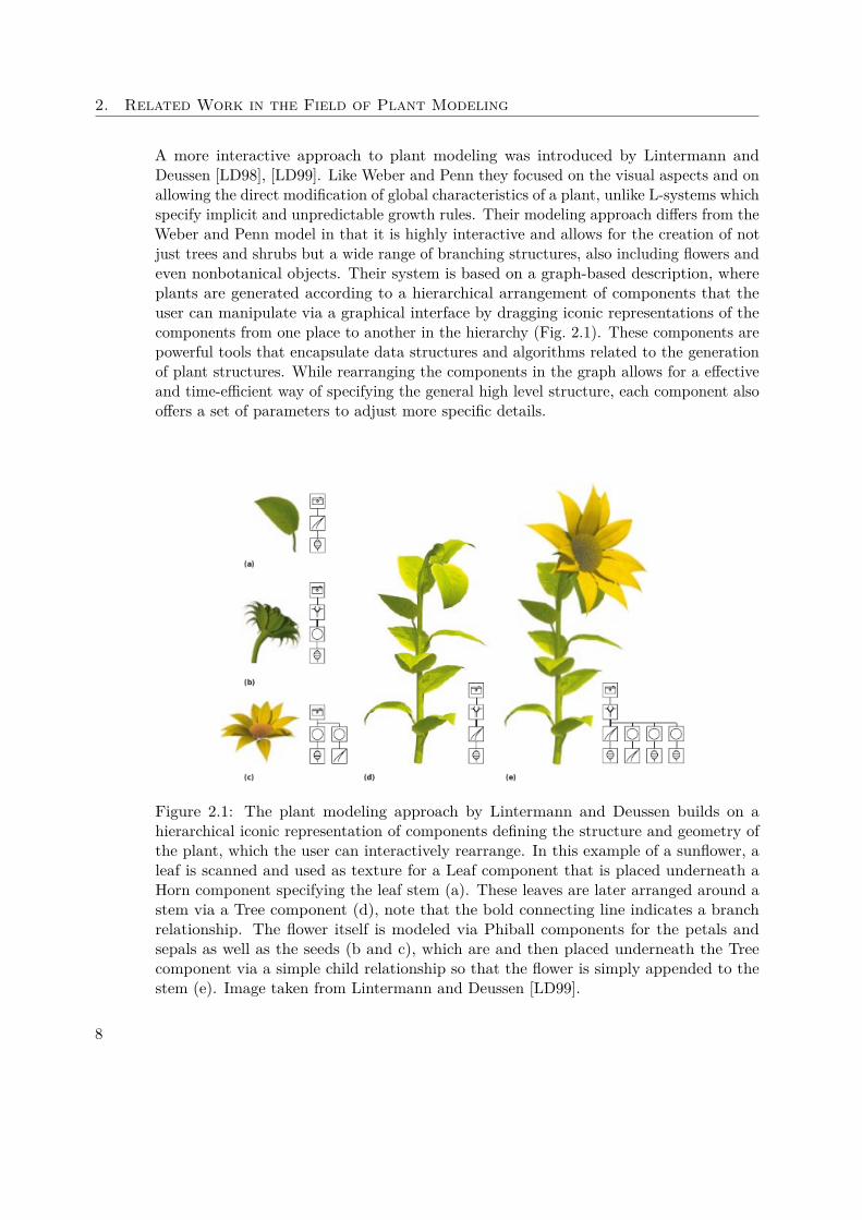
A more interactive approach to plant modeling was introduced by Lintermann andDeussen [LD98], [LD99]. Like Weber and Penn they focused on the visual aspects and onallowing the direct modification of global characteristics of a plant, unlike L-systems whichspecify implicit and unpredictable growth rules. Their modeling approach differs from theWeber and Penn model in that it is highly interactive and allows for the creation of notjust trees and shrubs but a wide range of branching structures, also including flowers andeven nonbotanical objects. Their system is based on a graph-based description, whereplants are generated according to a hierarchical arrangement of components that theuser can manipulate via a graphical interface by dragging iconic representations of thecomponents from one place to another in the hierarchy (Fig. 2.1). These components arepowerful tools that encapsulate data structures and algorithms related to the generationof plant structures. While rearranging the components in the graph allows for a effectiveand time-efficient way of specifying the general high level structure, each component alsooffers a set of parameters to adjust more specific details.

Figure 2.1: The plant modeling approach by Lintermann and Deussen builds on ahierarchical iconic representation of components defining the structure and geometry ofthe plant, which the user can interactively rearrange. In this example of a sunflower, aleaf is scanned and used as texture for a Leaf component that is placed underneath aHorn component specifying the leaf stem (a). These leaves are later arranged around astem via a Tree component (d), note that the bold connecting line indicates a branchrelationship. The flower itself is modeled via Phiball components for the petals andsepals as well as the seeds (b and c), which are and then placed underneath the Treecomponent via a simple child relationship so that the flower is simply appended to thestem (e). Image taken from Lintermann and Deussen [LD99].

8

2.3. Particle Systems and Space Colonialization

The types of components include some that define simple geometric primitives or morecomplex structures such as surfaces of revolution or the Horn component which defines asequence of point sets used as cross sections that can be oriented in various ways and arelater connected and triangulated to form a stem or twig. A Leaf component allows forinteractive modeling of leaves by adjusting polygonal curves and also allows to projecttextures.

The Tree component extends the Horn component by arranging its child components asbranches on itself, where the user can easily specify branch density, angular deviation etc.Other components that also create instances of subsequent components include Hydraand Wreath, creating a circular arrangement where instances are oriented perpendicularor parallel respectively. The Phiball component places components on a section of asphere according to the golden section, a common pattern in phyllotaxis.

Additionally, there are components to further adjust the final plant structure. TheFFD and HyperPatch components for free form deformation by specifying functions orinteractively moving controls points of a 3D patch, respectively. A Pruning componentcan be used to limit the growth to a specified CSG volume, either cutting or scalinggeometry for that purpose. Finally the World component defines global constraints toplant growth by simulation of gravitropism and phototropism, i.e. by specifying thetendency of growth to orient according to gravity or light fields. Further variation isintroduced by allowing each component parameter to be individually transformed by auser-specified function or a random factor. To model exceptions such as dead branches,components that iteratively create instances also hold a list of boolean flags, that for eachiteration number indicates whether an instance will be created or not. Thus an exceptioncould be introduced by switching of the flags e.g. for iteration numbers 2, 3, and 5, andusing another component that has these flags enabled and produced a different geometry.

All in all, the technique introduced by Lintermann and Deussen offers a highly effectivemeans of quickly modeling diverse plant structures of realistic appearance. According toan evaluation by Lintermann and Deussen [LD98] in two groups involving 18 inexperiencedusers, most of them found the component and hierarchy based modeling approach intuitive,yet found the great numbers of parameters a bit confusing. The groups were howeverable to model structures like a tulip in less than an hour, being allowed to ask questions.Experienced users were reported to be able to create convincing models of complex treeswithin 2 hours. Notably, existing component hierarchies can easily be reused to createvariations of existing trees in a few minutes.

2.3 Particle Systems and Space ColonializationTwo other techniques that shall be described here are based on particle systems andpoint clouds. Rodkaew and Chongstitvatana [RCSL03] presented a surprisingly simplemethod for modeling three dimensional branching structures yielding very plausibleresults. They first describe the synthesis of leaf venation patterns via particle systems ina two-dimensional space, which they then extend to the modeling of trees and shrubs,

9

2. Related Work in the Field of Plant Modeling

as well as root systems. For the purpose of modeling leaf venation, a boundary shapeis chosen in which particles are randomly distributed. Particles then iteratively movetoward the petiole (the leaf stalk) while being simultaneously attracted by the nearestneighboring particle: Simply adding the respective unit vectors and multiplying witha given step size is deemed sufficient for determining the particle displacement. Veinsthen correspond to the trails of the particles. When particles come close enough to eachother, they are merged to form a single particle with combined attributes. An abstractattribute called “energy” is initially assigned in uniform distribution to each particle, tomodel the thickness of veins determined as a function of this energy. As particles movetoward each other and merge, their energies are added up, leading to thicker veins asparticles move closer to the petiole, until eventually only one particle remains. The modelis easily extended to the three dimensional case. For the modeling of trees, Rodkaewand Chongstitvatana recommend distributing particles in a volume between an innerand an outer boundary shape. Leaves can then be placed at the initial particle positions.While not being suitable for some kind of plants, this method yields realistic visualmodels of leaf venation and tree branching structures from a very simple set of rules anda very limited set of parameters including the boundary shape determining the initialdistribution, the number of particles and their initial energy, the merging radius and themovement step size. To model the effect of light they employ a ray-tracing technique tosimulate light distribution, which can then be used to determine the density of initialparticles.

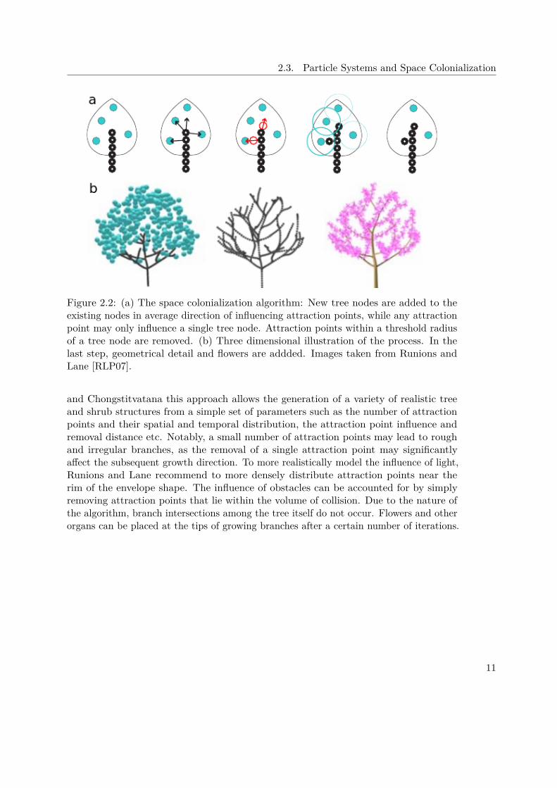
A similar approach was introduced by Runions and Lane [RLP07], who interestinglyalso based their model for trees on a model of leaf venation. They explicitly mentionthat the development of tree branches is often much more influenced by the competitionfor space and other environmental factors, as opposed to intrinsic branching patternsof the plant. Their method differs from that of Rodkaew and Chongstitvatana in thatbranches are formed in a base-to-leaves order. Very similarly, they also assume a threedimensional envelope shape as a boundary for the tree crown, yet instead of distributinginitial particles growing down from the tips to the base, the envelope is seeded withattraction points. These attraction points can be seen as indicators of empty space tobe filled by branch growth. The space colonialization algorithm described by Runionsand Lane treats the growing structure as a collection of tree nodes that grow towardthe attraction points, as illustrated in fig. 2.2. Starting from a single tree node at thebase, existing tree nodes are influenced by any number of attraction points, where anattraction point only influences its closest tree node (as in Voronoi partitioning), if it iswithin a radius of influence. For each node influenced by at least one attraction point, anew node is generated one step of constant distance away toward the arithmetic meandirection to all influencing attraction points. This direction of growth may be deliberatelybiased by another vector to account for tropisms and branch weight. Attraction pointsare removed as soon as a tree node is generated within a given threshold distance, toindicate that the space is filled. This process is repeated until all attraction pointshave been removed, no more nodes are within the radius of influence of any attractionpoint or a user specified number of iterations is reached. Like the model by Rodkaew

10

2.3. Particle Systems and Space Colonialization

Figure 2.2: (a) The space colonialization algorithm: New tree nodes are added to theexisting nodes in average direction of influencing attraction points, while any attractionpoint may only influence a single tree node. Attraction points within a threshold radiusof a tree node are removed. (b) Three dimensional illustration of the process. In thelast step, geometrical detail and flowers are addded. Images taken from Runions andLane [RLP07].

and Chongstitvatana this approach allows the generation of a variety of realistic treeand shrub structures from a simple set of parameters such as the number of attractionpoints and their spatial and temporal distribution, the attraction point influence andremoval distance etc. Notably, a small number of attraction points may lead to roughand irregular branches, as the removal of a single attraction point may significantlyaffect the subsequent growth direction. To more realistically model the influence of light,Runions and Lane recommend to more densely distribute attraction points near therim of the envelope shape. The influence of obstacles can be accounted for by simplyremoving attraction points that lie within the volume of collision. Due to the nature ofthe algorithm, branch intersections among the tree itself do not occur. Flowers and otherorgans can be placed at the tips of growing branches after a certain number of iterations.

11

CHAPTER 3Lindenmayer Systems

The formalism of Lindenmayer systems known today has been the result of manyyears of interdisciplinary research with contributions from several fields of study, mostnotably computer graphics and botany. As such, it has attracted interest for its possibleapplications both for image synthesis purposes and for scientific visualization.

As mentioned in the last chapter, there are other techniques of algorithmic botanythat may offer more effective means of generating plant models for artistic uses. WhileL-systems are very well capable of producing images evoking aesthetic pleasure in ahuman observer, they do not allow for intuitive artistic control in the modeling of plantswithout more interactive extensions. The beauty of L-systems lies not in artistic freedomof a human user, but much more in the astonishing diversity of patterns emerging fromthe procedural productions themselves. A small set of simple definitions and rules spicedwith a bit of pseudorandom variation can yield the most fascinating forms. As noted byPrusinkiewicz [Pru00], L-systems however are not so much a method to model the mereappearance of a plant, i.e. a “descriptive” model focused on the geometric definition ofplant shape. They much more fall into the category of “functional-structural” models,which try to reflect the physiological growth processes intrinsic to the development ofplant form. Plants can be described as modular structures consisting of individual units,such as branches, leaves and flowers. Instead of explicitly specifying the structure andarrangement of each individual modules in a grown plant, functional-structural modelstry to implicitly capture the growth of arbitrarily complex structures via a small set ofrules, describing the development of each class of module.

The original formulation of Lindenmayer systems is attributed to Aristid Lindenmayer,who in his work as a biologist was first and foremost inspired by the study of plantphysiology. In the year 1968 Lindenmayer published his studies on a mathematicalframework to simulate the development of simple multicellular organisms [Lin68]. Hisapproach is based on a parallel string rewriting method, in which an organism is definedby a string of symbols, sometimes called an L-string, from a limited alphabet that

13

3. Lindenmayer Systems

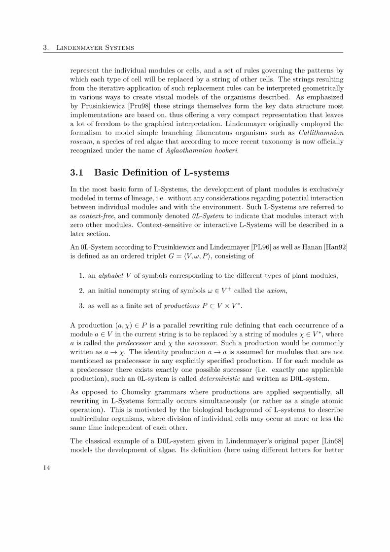
represent the individual modules or cells, and a set of rules governing the patterns bywhich each type of cell will be replaced by a string of other cells. The strings resultingfrom the iterative application of such replacement rules can be interpreted geometricallyin various ways to create visual models of the organisms described. As emphasizedby Prusinkiewicz [Pru98] these strings themselves form the key data structure mostimplementations are based on, thus offering a very compact representation that leavesa lot of freedom to the graphical interpretation. Lindenmayer originally employed theformalism to model simple branching filamentous organisms such as Callithamnionroseum, a species of red algae that according to more recent taxonomy is now officiallyrecognized under the name of Aglaothamnion hookeri.

3.1 Basic Definition of L-systemsIn the most basic form of L-Systems, the development of plant modules is exclusivelymodeled in terms of lineage, i.e. without any considerations regarding potential interactionbetween individual modules and with the environment. Such L-Systems are referred toas context-free, and commonly denoted 0L-System to indicate that modules interact withzero other modules. Context-sensitive or interactive L-Systems will be described in alater section.

An 0L-System according to Prusinkiewicz and Lindenmayer [PL96] as well as Hanan [Han92]is defined as an ordered triplet G = 〈V, ω, P 〉, consisting of

1. an alphabet V of symbols corresponding to the different types of plant modules,

2. an initial nonempty string of symbols ω ∈ V + called the axiom,

3. as well as a finite set of productions P ⊂ V × V ∗.

A production (a, χ) ∈ P is a parallel rewriting rule defining that each occurrence of amodule a ∈ V in the current string is to be replaced by a string of modules χ ∈ V ∗, wherea is called the predecessor and χ the successor. Such a production would be commonlywritten as a→ χ. The identity production a→ a is assumed for modules that are notmentioned as predecessor in any explicitly specified production. If for each module asa predecessor there exists exactly one possible successor (i.e. exactly one applicableproduction), such an 0L-system is called deterministic and written as D0L-system.

As opposed to Chomsky grammars where productions are applied sequentially, allrewriting in L-Systems formally occurs simultaneously (or rather as a single atomicoperation). This is motivated by the biological background of L-systems to describemulticellular organisms, where division of individual cells may occur at more or less thesame time independent of each other.

The classical example of a D0L-system given in Lindenmayer’s original paper [Lin68]models the development of algae. Its definition (here using different letters for better

14

3.1. Basic Definition of L-systems

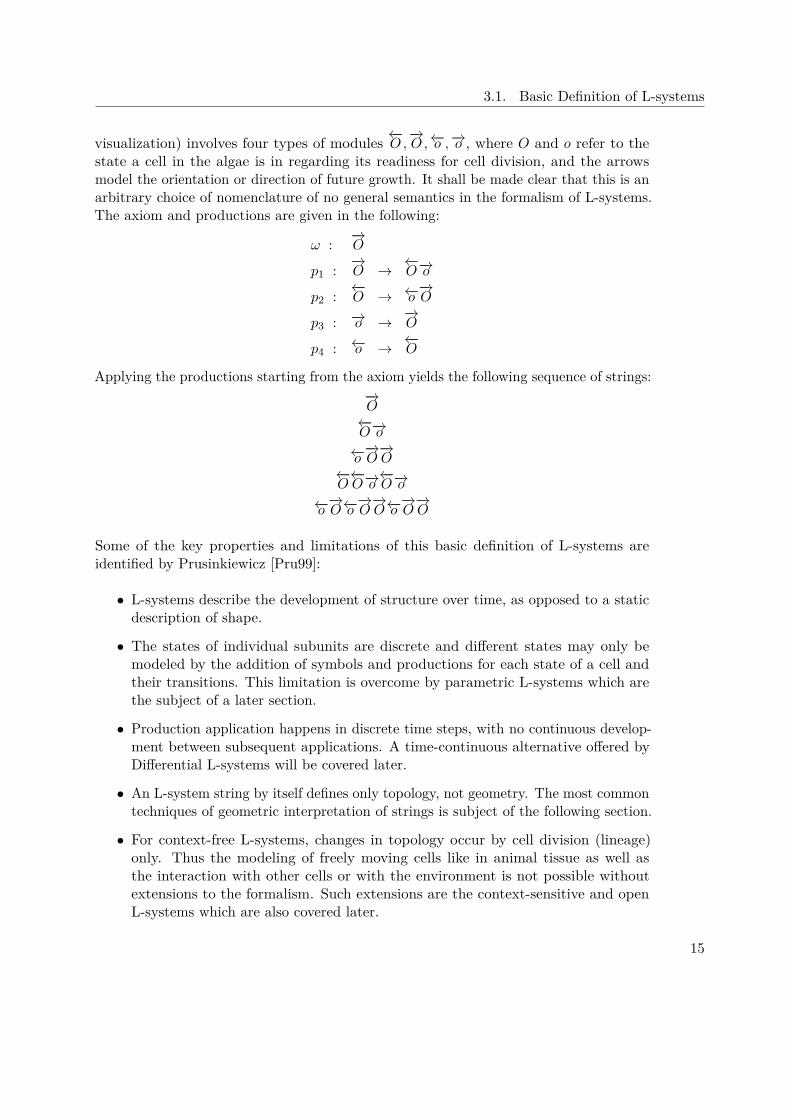
visualization) involves four types of modules ←−O,−→O,←−o ,−→o , where O and o refer to thestate a cell in the algae is in regarding its readiness for cell division, and the arrowsmodel the orientation or direction of future growth. It shall be made clear that this is anarbitrary choice of nomenclature of no general semantics in the formalism of L-systems.The axiom and productions are given in the following:

ω : −→O

p1 : −→O →←−O−→o

p2 : ←−O → ←−o−→O

p3 : −→o →−→O

p4 : ←−o →←−O

Applying the productions starting from the axiom yields the following sequence of strings:−→O←−O−→o←−o−→O−→O

←−O←−O−→o←−O−→o

←−o−→O←−o−→O−→O←−o−→O−→O

Some of the key properties and limitations of this basic definition of L-systems areidentified by Prusinkiewicz [Pru99]:

• L-systems describe the development of structure over time, as opposed to a staticdescription of shape.

• The states of individual subunits are discrete and different states may only bemodeled by the addition of symbols and productions for each state of a cell andtheir transitions. This limitation is overcome by parametric L-systems which arethe subject of a later section.

• Production application happens in discrete time steps, with no continuous develop-ment between subsequent applications. A time-continuous alternative offered byDifferential L-systems will be covered later.

• An L-system string by itself defines only topology, not geometry. The most commontechniques of geometric interpretation of strings is subject of the following section.

• For context-free L-systems, changes in topology occur by cell division (lineage)only. Thus the modeling of freely moving cells like in animal tissue as well asthe interaction with other cells or with the environment is not possible withoutextensions to the formalism. Such extensions are the context-sensitive and openL-systems which are also covered later.

15

3. Lindenmayer Systems

3.1.1 Branching Structures and Bracketed L-systems

So far no specifications have been made regarding any methodology to define branchingstructures, which needless to say is of central importance to the description of plantstructure. Lindenmayer in his original work [Lin68] proposed a notation of bracketedstrings, known as bracketed L-systems. It involves the addition of left and right brackets,“[” and “]” as special symbols to the productions. Each opening left bracket indicatesthe start of new branch attached to the module to its left, containing all subsequentmodules up to the next unmatched closing right bracket. More specifically, whenever aright bracket is found while traversing the string from left to right, it is matched withthe last unmatched occurrence of a left bracket. Obviously for each left bracket thereshould be a matching right bracket. The nesting of matching pairs is possible, allowingfor the definition of branches of higher order. The interpretation of bracketed strings isfacilitated by the use of stack data structures, as described in the next section, whichalso demonstrates possible geometric interpretations of bracketed L-systems.

3.2 Interpretation of Strings via Turtle GraphicsTo be used for the visualization of plant models, the strings produced by an L-systemneed to be interpreted graphically. By themselves they only describe the topology ofmodules, i.e. how they are arranged relative to each other within the structure, but notwhere in space they shall be positioned, how they shall be oriented etc.

As noted by Prusinkiewicz [Pru99], two different approaches for the geometric interpreta-tion have been suggested:

• One might keep the specification of any geometric information separate from theproduction of modules, thus leaving the details about how each module or successionsof modules shall be positioned and oriented geometrically in the interpretation stepentirely to the system interpreting the strings. This would however make it verydifficult to achieve consistent results on different systems without sharing additionalinterpretation instructions. More importantly however, the geometric aspects ofplant growth would be separate from the development process itself.

• Another approach would be to introduce special symbols to be used as standardizedinstructions for the interpreting system. These symbols would be added or removedas part of the production process itself and thus would allow the specificationof geometric detail right within the L-system formalism, allowing a predictableinterpretation.

Most L-system implementations today include symbols related entirely to the geometricaland graphical interpretation as a central part of the production process and use atechnique commonly known as turtle interpretation, that is based on the turtle graphicsmethodology. Turtle graphics was first used as part of the educational programming

16

3.2. Interpretation of Strings via Turtle Graphics

language LOGO, where the turtle was used to conceptualize a relative cursor, thatwould draw lines as it moved around the screen like a pen-carrying turtle. The turtle iscontrolled by a sequence of commands that would change its state and create a figure tobe drawn on the screen.

The state of the turtle consists of its position ~P in 3D space, as well three perpendicularunit vectors heading ~H, left ~L and up ~U defining its orientation, i.e. its local coordinatesystem, where ~H × ~L = ~U , as well as some drawing attributes like color and line width.Using homogeneous coordinates, the 4 vectors can be conveniently represented by a 4x4matrix allowing for efficient state transformations.

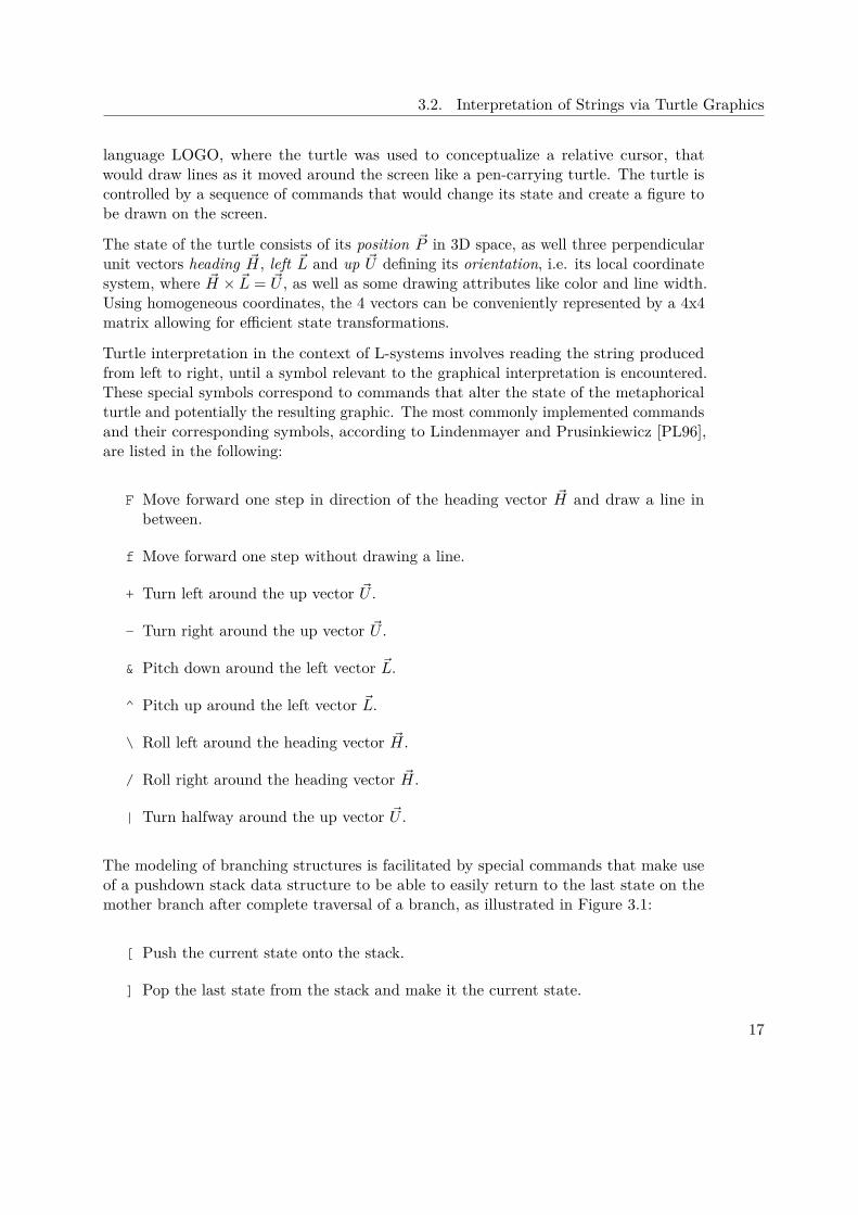
Turtle interpretation in the context of L-systems involves reading the string producedfrom left to right, until a symbol relevant to the graphical interpretation is encountered.These special symbols correspond to commands that alter the state of the metaphoricalturtle and potentially the resulting graphic. The most commonly implemented commandsand their corresponding symbols, according to Lindenmayer and Prusinkiewicz [PL96],are listed in the following:

F Move forward one step in direction of the heading vector ~H and draw a line inbetween.

f Move forward one step without drawing a line.

+ Turn left around the up vector ~U .

- Turn right around the up vector ~U .

& Pitch down around the left vector ~L.

^ Pitch up around the left vector ~L.

\ Roll left around the heading vector ~H.

/ Roll right around the heading vector ~H.

| Turn halfway around the up vector ~U .

The modeling of branching structures is facilitated by special commands that make useof a pushdown stack data structure to be able to easily return to the last state on themother branch after complete traversal of a branch, as illustrated in Figure 3.1:

[ Push the current state onto the stack.

] Pop the last state from the stack and make it the current state.

17

3. Lindenmayer Systems

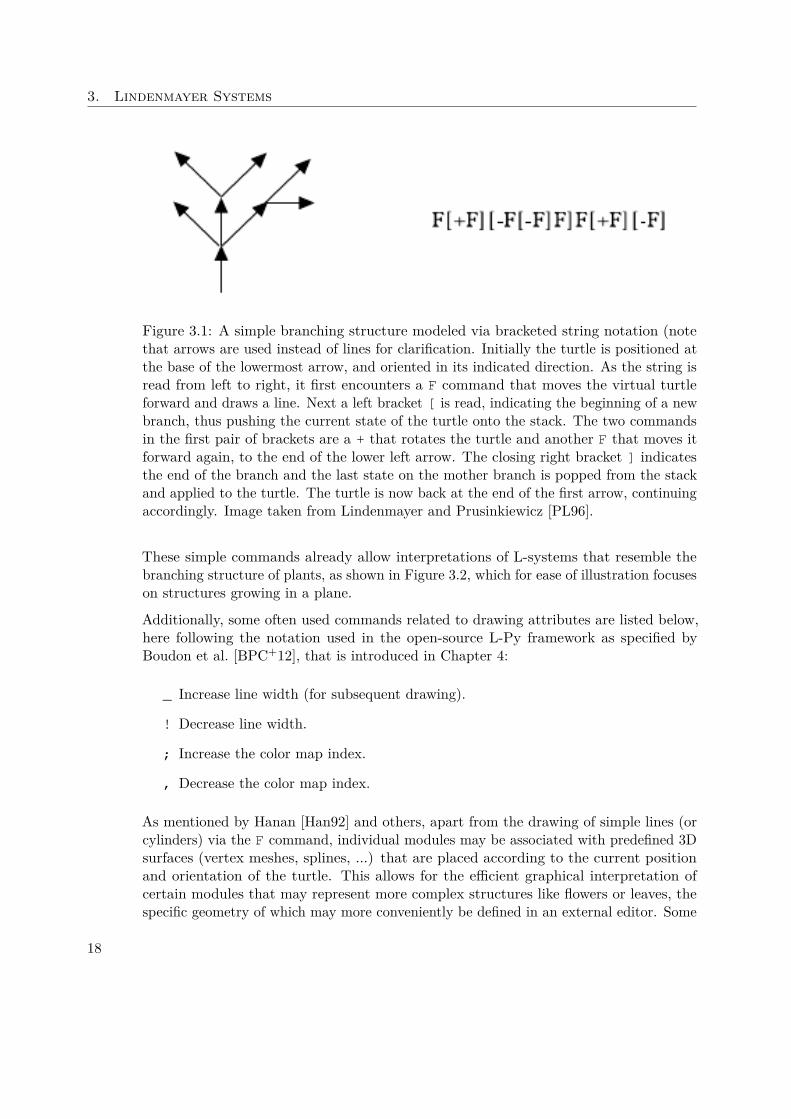
Figure 3.1: A simple branching structure modeled via bracketed string notation (notethat arrows are used instead of lines for clarification. Initially the turtle is positioned atthe base of the lowermost arrow, and oriented in its indicated direction. As the string isread from left to right, it first encounters a F command that moves the virtual turtleforward and draws a line. Next a left bracket [ is read, indicating the beginning of a newbranch, thus pushing the current state of the turtle onto the stack. The two commandsin the first pair of brackets are a + that rotates the turtle and another F that moves itforward again, to the end of the lower left arrow. The closing right bracket ] indicatesthe end of the branch and the last state on the mother branch is popped from the stackand applied to the turtle. The turtle is now back at the end of the first arrow, continuingaccordingly. Image taken from Lindenmayer and Prusinkiewicz [PL96].

These simple commands already allow interpretations of L-systems that resemble thebranching structure of plants, as shown in Figure 3.2, which for ease of illustration focuseson structures growing in a plane.

Additionally, some often used commands related to drawing attributes are listed below,here following the notation used in the open-source L-Py framework as specified byBoudon et al. [BPC+12], that is introduced in Chapter 4:

_ Increase line width (for subsequent drawing).

! Decrease line width.

; Increase the color map index.

, Decrease the color map index.

As mentioned by Hanan [Han92] and others, apart from the drawing of simple lines (orcylinders) via the F command, individual modules may be associated with predefined 3Dsurfaces (vertex meshes, splines, ...) that are placed according to the current positionand orientation of the turtle. This allows for the efficient graphical interpretation ofcertain modules that may represent more complex structures like flowers or leaves, thespecific geometry of which may more conveniently be defined in an external editor. Some

18

3.3. Stochastic L-systems

implementations also allow the specification of mesh surfaces on a vertex level withinL-systems themselves via specialized commands that are however beyond the scope ofthis chapter.

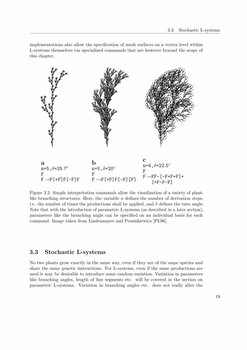
Figure 3.2: Simple interpretation commands allow the visualization of a variety of plant-like branching structures. Here, the variable n defines the number of derivation steps,i.e. the number of times the productions shall be applied, and δ defines the turn angle.Note that with the introduction of parametric L-systems (as described in a later section),parameters like the branching angle can be specified on an individual basis for eachcommand. Image taken from Lindenmayer and Prusinkiewicz [PL96].

3.3 Stochastic L-systemsNo two plants grow exactly in the same way, even if they are of the same species andshare the same genetic instructions. For L-systems, even if the same productions areused it may be desirable to introduce some random variation. Variation in parameterslike branching angles, length of line segments etc. will be covered in the section onparametric L-systems. Variation in branching angles etc. does not really alter the

19

3. Lindenmayer Systems

topology of the structures produced. Much more striking random deviations can beachieved by randomly choosing between different productions to be applied for a givenpredecessor. For this purpose, the notion of stochastic L-systems was introduced byEichhorst and Savitch [ES80], where productions are assigned a probability in (0, 1] suchthat the probabilities of all productions sharing a common predecessor sum up to 1. Ifmultiple productions are specified for a given predecessor, the production to be applied isselected randomly according to the given probability distribution. If only one productionis specified for a module, the probability of its selection is 1.

The probabilities may be commonly written on top of the derivation symbol (productionarrow) or at the end of the production following a colon:

ω : F

p1 : F .33−−→ F[+F]F[−F]F

p2 : F .33−−→ F[+F]F

p3 : F .34−−→ F[−F]F

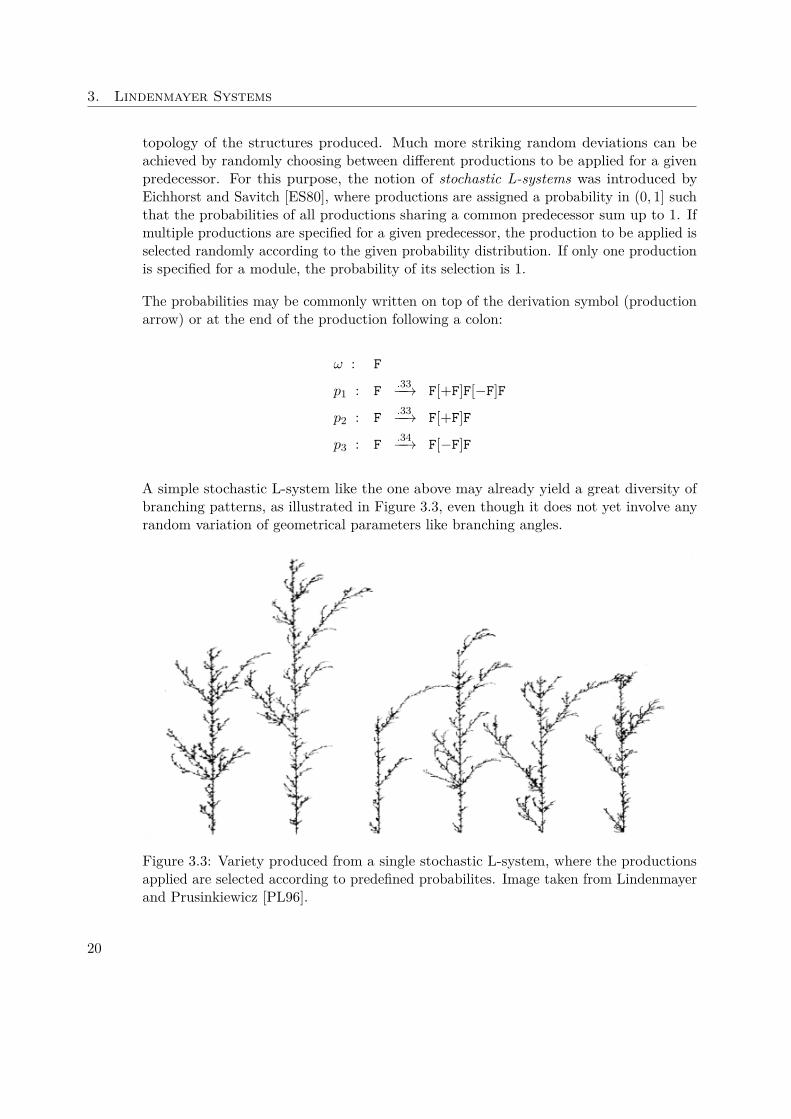
A simple stochastic L-system like the one above may already yield a great diversity ofbranching patterns, as illustrated in Figure 3.3, even though it does not yet involve anyrandom variation of geometrical parameters like branching angles.

Figure 3.3: Variety produced from a single stochastic L-system, where the productionsapplied are selected according to predefined probabilites. Image taken from Lindenmayerand Prusinkiewicz [PL96].

20

3.4. Parametric L-systems

3.4 Parametric L-systems

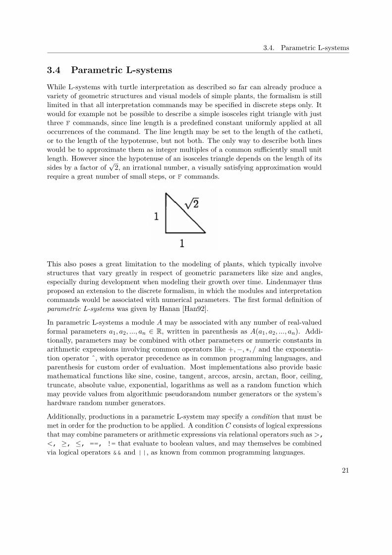
While L-systems with turtle interpretation as described so far can already produce avariety of geometric structures and visual models of simple plants, the formalism is stilllimited in that all interpretation commands may be specified in discrete steps only. Itwould for example not be possible to describe a simple isosceles right triangle with justthree F commands, since line length is a predefined constant uniformly applied at alloccurrences of the command. The line length may be set to the length of the catheti,or to the length of the hypotenuse, but not both. The only way to describe both lineswould be to approximate them as integer multiples of a common sufficiently small unitlength. However since the hypotenuse of an isosceles triangle depends on the length of itssides by a factor of

√2, an irrational number, a visually satisfying approximation would

require a great number of small steps, or F commands.

This also poses a great limitation to the modeling of plants, which typically involvestructures that vary greatly in respect of geometric parameters like size and angles,especially during development when modeling their growth over time. Lindenmayer thusproposed an extension to the discrete formalism, in which the modules and interpretationcommands would be associated with numerical parameters. The first formal definition ofparametric L-systems was given by Hanan [Han92].

In parametric L-systems a module A may be associated with any number of real-valuedformal parameters a1, a2, ..., an ∈ R, written in parenthesis as A(a1, a2, ..., an). Addi-tionally, parameters may be combined with other parameters or numeric constants inarithmetic expressions involving common operators like +,−, ∗, / and the exponentia-tion operator ˆ, with operator precedence as in common programming languages, andparenthesis for custom order of evaluation. Most implementations also provide basicmathematical functions like sine, cosine, tangent, arccos, arcsin, arctan, floor, ceiling,truncate, absolute value, exponential, logarithms as well as a random function whichmay provide values from algorithmic pseudorandom number generators or the system’shardware random number generators.

Additionally, productions in a parametric L-system may specify a condition that must bemet in order for the production to be applied. A condition C consists of logical expressionsthat may combine parameters or arithmetic expressions via relational operators such as >,<, ≥, ≤, ==, != that evaluate to boolean values, and may themselves be combinedvia logical operators && and ||, as known from common programming languages.

21

3. Lindenmayer Systems

Productions (a,C, χ) with predecessor a, successor χ and condition C are commonlywritten as a : C → χ, like in the following example:

A(s, t) : s/2 < 7 && t < 4 → B(s ∗ 2)CD(sˆ2, t− 2)

A production will match and be applied to a module if the following three conditions canbe satisfied: The symbol of the production predecessor must be the same as the symbolof the module, the number of actual parameters (arguments) given by the module mustbe equal to the number of formal parameters specified by the production predecessor, andthe condition of the production must be met. The production given above would match amodule A(4, 3), since the symbol and the number of formal parameters of the productionpredecessor match the symbol and the number of arguments of the module, and thecondition evaluates to true for the given arguments. After evaluation of the parametersin the successor, the module is replaced by the resulting string B(8)CD(16, 1). In thisexample, the module C does not have any parameters. It shall be noted that for drawingcommands, parameters may have different meaning depending on the implementation.The commands _ and ! to increase and decrease line width for example are often assumedto both set the line width to a given value if a parameter argument is given.

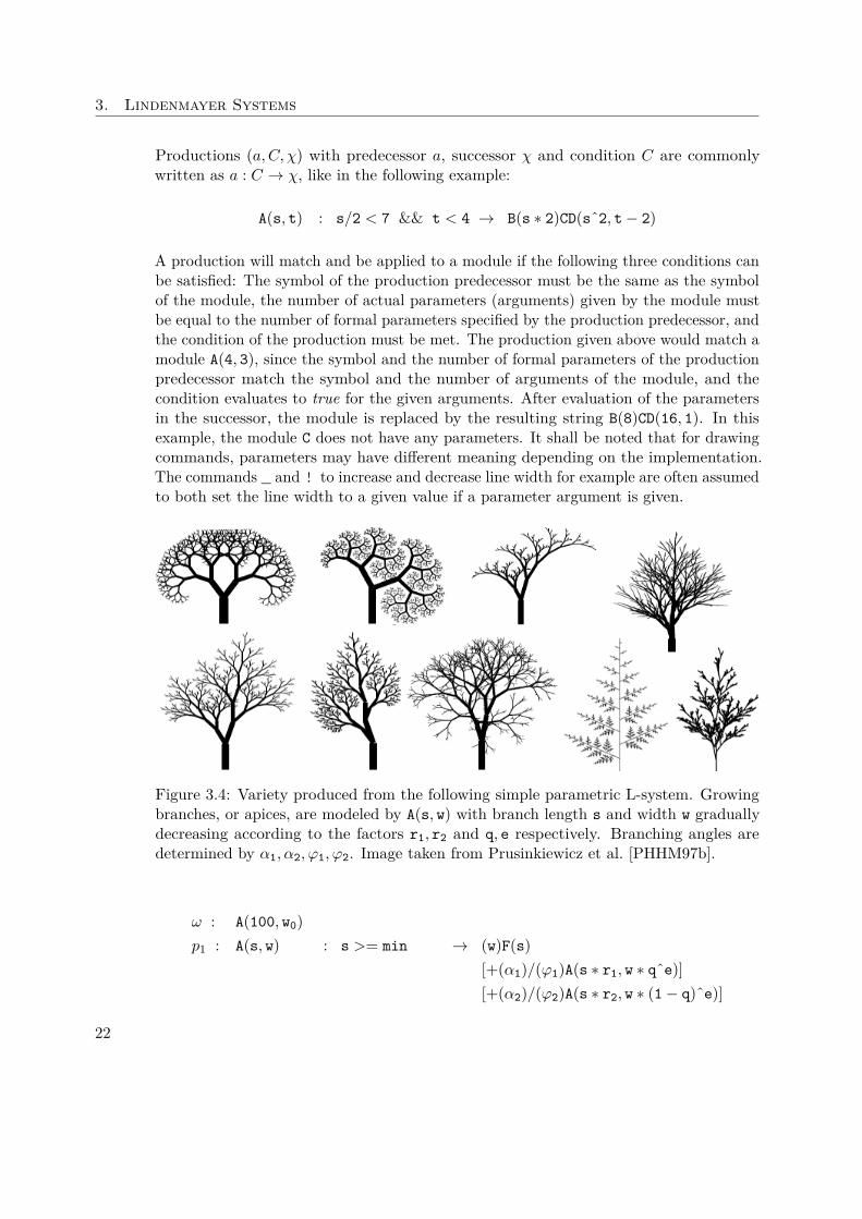
Figure 3.4: Variety produced from the following simple parametric L-system. Growingbranches, or apices, are modeled by A(s, w) with branch length s and width w graduallydecreasing according to the factors r1, r2 and q, e respectively. Branching angles aredetermined by α1, α2, ϕ1, ϕ2. Image taken from Prusinkiewicz et al. [PHHM97b].

ω : A(100, w0)p1 : A(s, w) : s >= min → (w)F(s)

[+(α1)/(ϕ1)A(s ∗ r1, w ∗ qˆe)][+(α2)/(ϕ2)A(s ∗ r2, w ∗ (1− q)ˆe)]

22

3.5. Context-sensitive L-systems

3.5 Context-sensitive L-systemsThe formalism thus far only accounted for the propagation of information via lineage,i.e. from a module to its successor. The exchange of information between neighboringmodules in the structure (endogenous interaction) and with external structures simulatingthe environment (exogenous interaction) was not considered in the model. L-systemsare however very well capable of modeling both types of interaction. This section shallexplore the simulation of endogenous interaction via an extension to L-systems known ascontext-sensitive L-systems or interactive L-systems (IL-systems).

The capability of modeling the interaction between modules of a growing structure is anessential aspect of the biologically motivated formulation of L-systems. As discussed byPrusinkiewicz et al. [PHHM97a], it allows the description of complex dynamic phenomenasuch as the propagation of signals or growth hormones that control the morphogeneticdevelopment of a plant, the distribution and flux of resources (minerals, water, photosyn-thates) among the growing structure or the response of a plant to pathogens like certaininsects. While such models are still far from biologically accurate descriptions of theprocesses mentioned, they allow visualizations of interaction for educative purposes andto test hypotheses by visual comparison of simulated models based on empirical dataof the actual structures. The expressive power of context-sensitive L-systems clearlydistinguishes them from purely geometric models.

A module in a string may have a left and a right context, given by the modules toits left and to its right. Depending on whether just one side or both are considered,context-sensitive L-systems are also referred to as 1L-systems or 2L-systems, respectively.The predecessor of a production in a 2L-system may specify a left and / or right contextas strings of modules, and will be applied to a module if it matches the actual context ofa module. The common syntax is lc < a > rc : C→ χ, where the triplet (lc, a, rc) isthe predecessor that includes the left and right context lc and rc, C is the condition,and χ the successor. a is called the strict predecessor, that is going to be replaced onproduction application. While the strict predecessor must be a single module, the leftand right context may involve a string of modules.

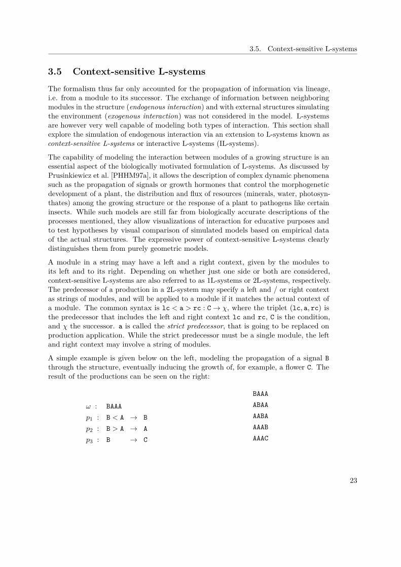
A simple example is given below on the left, modeling the propagation of a signal Bthrough the structure, eventually inducing the growth of, for example, a flower C. Theresult of the productions can be seen on the right:

ω : BAAA

p1 : B < A → B

p2 : B > A → A

p3 : B → C

BAAA

ABAA

AABA

AAAB

AAAC

23

3. Lindenmayer Systems

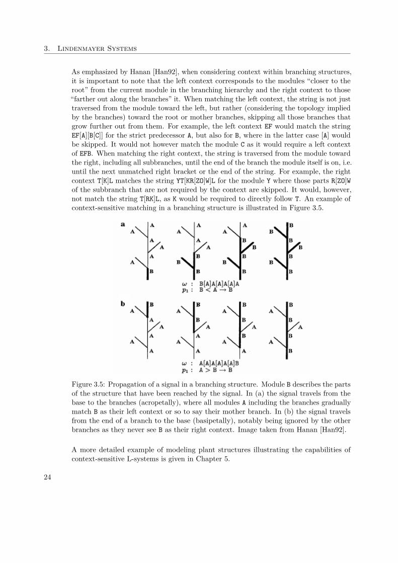
As emphasized by Hanan [Han92], when considering context within branching structures,it is important to note that the left context corresponds to the modules “closer to theroot” from the current module in the branching hierarchy and the right context to those“farther out along the branches” it. When matching the left context, the string is not justtraversed from the module toward the left, but rather (considering the topology impliedby the branches) toward the root or mother branches, skipping all those branches thatgrow further out from them. For example, the left context EF would match the stringEF[A][B[C]] for the strict predecessor A, but also for B, where in the latter case [A] wouldbe skipped. It would not however match the module C as it would require a left contextof EFB. When matching the right context, the string is traversed from the module towardthe right, including all subbranches, until the end of the branch the module itself is on, i.e.until the next unmatched right bracket or the end of the string. For example, the rightcontext T[K]L matches the string YT[KR[ZO]W]L for the module Y where those parts R[ZO]Wof the subbranch that are not required by the context are skipped. It would, however,not match the string T[RK]L, as K would be required to directly follow T. An example ofcontext-sensitive matching in a branching structure is illustrated in Figure 3.5.

Figure 3.5: Propagation of a signal in a branching structure. Module B describes the partsof the structure that have been reached by the signal. In (a) the signal travels from thebase to the branches (acropetally), where all modules A including the branches graduallymatch B as their left context or so to say their mother branch. In (b) the signal travelsfrom the end of a branch to the base (basipetally), notably being ignored by the otherbranches as they never see B as their right context. Image taken from Hanan [Han92].

A more detailed example of modeling plant structures illustrating the capabilities ofcontext-sensitive L-systems is given in Chapter 5.

24

3.6. Other Variants and Extensions

3.6 Other Variants and ExtensionsVarious extensions to the L-system formalism exist beyond those covered so far. Whilenot all of them can be demonstrated in this thesis, this section shall give a short overviewover some of the other commonly known methodologies in the field. A good overviewthat includes other extensions is given by Prusinkiewicz [Pru99].

3.6.1 Shedding of Branches

Sometimes it can be useful to be able to remove a large number of different modulesat once, without requiring individual productions for the removal of each one of them.Plants may shed branches or other organs at certain stages of their development, orloose them due to pruning. To facilitate the simulation of such processes, Hanan [Han92]introduced the cut symbol %. When encountered in a string, all symbols of the currentbranch (i.e. up to the next unmatched right bracket or the end of the string) wouldbe skipped, and thus rendered invisible to production application. For example, thestring AB[C%DE[FG]H]I[%JK]L%MNO would be read as AB[C]I[]L unless the cut symbols wereremoved.

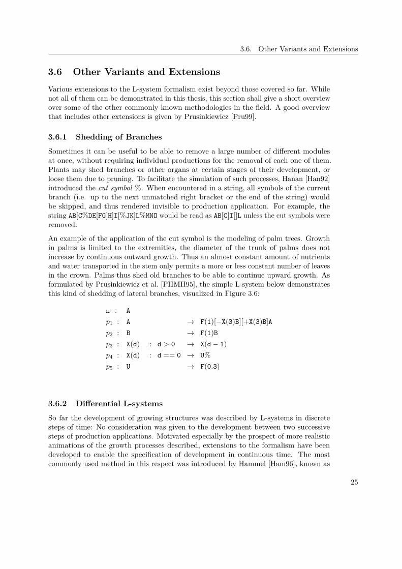
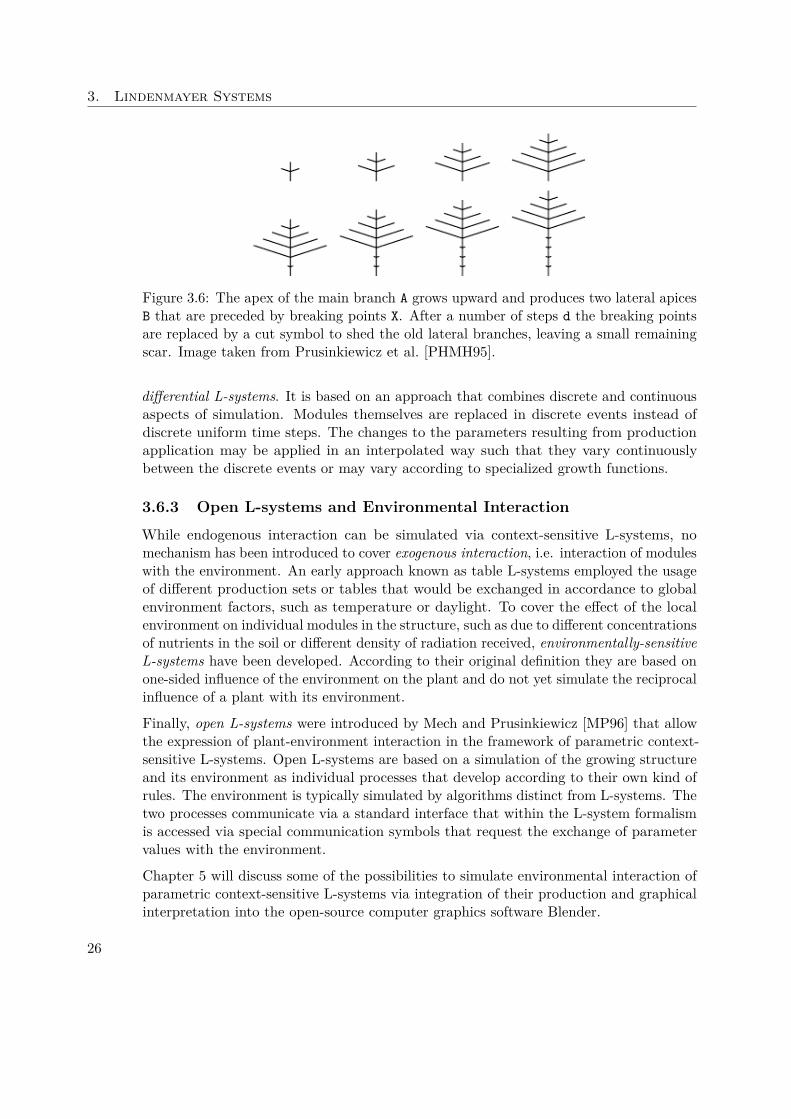
An example of the application of the cut symbol is the modeling of palm trees. Growthin palms is limited to the extremities, the diameter of the trunk of palms does notincrease by continuous outward growth. Thus an almost constant amount of nutrientsand water transported in the stem only permits a more or less constant number of leavesin the crown. Palms thus shed old branches to be able to continue upward growth. Asformulated by Prusinkiewicz et al. [PHMH95], the simple L-system below demonstratesthis kind of shedding of lateral branches, visualized in Figure 3.6:

ω : A

p1 : A → F(1)[−X(3)B][+X(3)B]Ap2 : B → F(1)Bp3 : X(d) : d > 0 → X(d− 1)p4 : X(d) : d == 0 → U%p5 : U → F(0.3)

3.6.2 Differential L-systems

So far the development of growing structures was described by L-systems in discretesteps of time: No consideration was given to the development between two successivesteps of production applications. Motivated especially by the prospect of more realisticanimations of the growth processes described, extensions to the formalism have beendeveloped to enable the specification of development in continuous time. The mostcommonly used method in this respect was introduced by Hammel [Ham96], known as

25

3. Lindenmayer Systems

Figure 3.6: The apex of the main branch A grows upward and produces two lateral apicesB that are preceded by breaking points X. After a number of steps d the breaking pointsare replaced by a cut symbol to shed the old lateral branches, leaving a small remainingscar. Image taken from Prusinkiewicz et al. [PHMH95].

differential L-systems. It is based on an approach that combines discrete and continuousaspects of simulation. Modules themselves are replaced in discrete events instead ofdiscrete uniform time steps. The changes to the parameters resulting from productionapplication may be applied in an interpolated way such that they vary continuouslybetween the discrete events or may vary according to specialized growth functions.

3.6.3 Open L-systems and Environmental Interaction

While endogenous interaction can be simulated via context-sensitive L-systems, nomechanism has been introduced to cover exogenous interaction, i.e. interaction of moduleswith the environment. An early approach known as table L-systems employed the usageof different production sets or tables that would be exchanged in accordance to globalenvironment factors, such as temperature or daylight. To cover the effect of the localenvironment on individual modules in the structure, such as due to different concentrationsof nutrients in the soil or different density of radiation received, environmentally-sensitiveL-systems have been developed. According to their original definition they are based onone-sided influence of the environment on the plant and do not yet simulate the reciprocalinfluence of a plant with its environment.

Finally, open L-systems were introduced by Mech and Prusinkiewicz [MP96] that allowthe expression of plant-environment interaction in the framework of parametric context-sensitive L-systems. Open L-systems are based on a simulation of the growing structureand its environment as individual processes that develop according to their own kind ofrules. The environment is typically simulated by algorithms distinct from L-systems. Thetwo processes communicate via a standard interface that within the L-system formalismis accessed via special communication symbols that request the exchange of parametervalues with the environment.

Chapter 5 will discuss some of the possibilities to simulate environmental interaction ofparametric context-sensitive L-systems via integration of their production and graphicalinterpretation into the open-source computer graphics software Blender.

26

3.6. Other Variants and Extensions

3.6.4 Genetic / Evolutionary Approaches

One last topic that shall be briefly mentioned is the use of genetic algorithms as knownfrom search, optimization and machine learning problems. L-systems modeled by humandesigners typically undergo a process of artificial evolution, where changes are made toproductions and the results evaluated to select the model that best fits the requirements. Afirst approach to automatically simulate this process of evolution, by inducing mutations toreach a greater variety of productions to choose from, was presented by MacKenzie [Mac93].He demonstrated the use of common genetic algorithms to optimize L-system productionsbased on criteria such as the amount of light received by a growing structure andsimilar. Another method was introduced by Burt [Bur13], as a kind of InteractiveEvolutionary Computation technique, where the user would guide the evolutionaryprocess by interactively selecting from a visualized set of variations produced from thecurrent productions, to be used as the starting point for the next round of mutations.Lastly it must be noted that, while these approaches are based on processes known fromthe development of genes via evolutionary processes, they operate on a highly abstractlevel far from the complexities of actual plant genetics.

27

CHAPTER 4Integrating the L-Py Framework

as an Add-on for Blender

One of the steps relating to the practical part of this bachelor thesis was to bring theexpressive power and aesthetic beauty enabled by L-systems to Blender, an open-source3D computer graphics software sustained by a broad community of users in many fields,with applications as diverse as animated films, architectural and scientific visualization,3D printing and game design. [FtBC17c].

Designing a full implemention of L-systems from the ground up would be beyond thescope of this thesis and would not be viable, especially since the main goal of this thesisis to discuss possible advantages or disadvantages of an integration in Blender, not somuch the details of possible implementations. Therefore, an existing implementationis used and adapted for use as an add-on for Blender. Regarding implementations forPython, the L-Py L-system simulation framework described in the next section can beconsidered the most feature-rich option available.

This chapter shall give a short introduction to the L-Py framework and the BlenderPython API, and will then focus on describing the steps taken to implement Lindenmaker,a small wrapper add-on of L-Py for Blender, as well as giving an overview on its mainfeatures and user interface. This chapter also discusses potential advantages of L-Pyintegration in Blender from a more theoretical standpoint. To test this potential onpractical examples, applications of the add-on for the modeling of the visual structure ofplants as well as their interaction with a Blender scene will be the subject of Chapter 5.

Lindenmaker employs an adapted version of L-Py as the basis for L-string production,while aspects related to the graphical turtle interpretation are rewritten from the groundup via the Blender Python API. The core functionality of Blender, written in C andC++, can be extended via the Blender Python API, allowing access to most operatorsand data that is accessible to the user via the GUI. Extensions can be made in the form

29

4. Integrating the L-Py Framework as an Add-on for Blender

of small Python scripts up to full-fledged add-ons that may be shipped with the officalBlender release.

The software source code for both the adapted version of L-Py as well as the Lindenmakeradd-on is publicly available under an open source license on GitHub:https://github.com/mangostaniko/lpy-lsystems-blender-addon. [Leo17]

To summarize, the steps taken to integrate parametric context-sensitive L-systems inBlender can be outlined as in the following:

• Adapt the L-Py L-system framework so that it can be used as a Python module inthe Blender Python interpreter

• Write a Blender add-on that forms a wrapper around the L-string productioncapabilities of L-Py and offers graphical turtle interpretation using the BlenderPython API, including special functionality related specifically to advantages ofintegration in Blender, most notably use of modeled objects and environmentalinteraction with the Blender scene.

Note that to avoid ambiguity in the context of programming languages, the term L-stringis used throughout this section to refer to the string of modules an L-system operates on.

4.1 L-Py: An open-source L-system Framework forPython

L-Py is an open-source framework and library for the simulation of L-systems based onPython, developed by Boudon et al. [BPC+12].

Prior to L-Py, numerous L-system implementations have been developed, most of thembased on statically typed languages. One of the most significant contributions was the pfg(plant and fractal generator) by Prusinkiewicz and Hanan, which was the central part ofthe Virtual Laboratory plant simulation framework described by Mercer et al. [MPH90],and its successor cpfg (pfg with continuous parameters) by Hanan [Han92]. Pfg and cpfgfirst allowed the use of general programming language constructs in the specification ofparametric context-sensitive L-systems, including local and global variables, functionsand flow-control statements [PHM99]. Notably, pfg and cpfg did not build upon anexisting framework for an imperative language, but rather used their own implementationof an interpreter for C-like language constructs to extend the formalism of L-systems. Forsimplicity, only a subset of features of the C language are included in the cpfg language.

A different approach was taken by Karwowski and Prusinkiewicz [KP03] in developingthe L+C language and the corresponding lpfg simulation framework. The L+C languageis fully based on C++ and uses features of the language itself, like classes, libraries etc.to extend its syntax to the formalism of L-systems. L+C thus has the same expressivepower as the C++ language and allows for more complex L-system constructs such as

30

4.1. L-Py: An open-source L-system Framework for Python

module parameters with compound data types (structures), as described by Karwowskiet al. [PKL07]. Both cpfg and lpfg are part of the current implementation of the VirtualLaboratory suite, which is also distributed with a different user interface under thename of L-studio [Pru04]. Another notable contribution was made by Kniemeyer andKurth [KK08] with XL (eXtended L-system language), which is based on the interpretedJava language, focusing on cross-platform portability. All frameworks mentioned so farare however still based on statically typed languages, contrary to the dynamically typedPython language employed by L-Py.

The core of L-Py, as described by Boudon et al. [BPC+12], is itself written in C++ forimproved performance of compiled binaries. To benefit from the flexibility, simple syntaxand concise high-level expressions of the dynamically typed and interpreted Pythonlanguage, the core features are exposed as a Python module via the Boost.Python library,which can provide an almost seamless mapping of the most relevant C++ constructs toPython constructs. Apart from the considerably more shallow learning curve and greatexpressive power of Python, another significant advantage of its dynamic nature is thatonce the L-Py C++ framework itself has been compiled to a Python module, users ofthe framework are not required to compile their L-system definitions prior to use.

The L-Py interpreter compiles the code of an L-system model (typically stored in afile with extension .lpy) to pure Python code via the L-Py parser. Predecessors arestored in dedicated data structures, and rules are reformulated as Python functions.The interpreter then iteratively applies production rules to the previously producedL-string, starting with the axiom. To this end, the L-string is parsed and scanned formodules that match a predecessor in any of the defined productions by module name andnumber of parameters. Once a match is found, the respective production is applied bycalling its corresponding Python function and appending the string of modules it returns(the successor of the production) to the L-string resulting from the current productionapplication step. Thanks to the dynamic language evaluation of Python, introspectionand runtime modification of L-system models is possible.

The L-Py source code and precompiled binaries are made available as part of the OpenAleadistribution developed at INRIA. OpenAlea comprises as set of tools related to plantarchitecture analysis and modeling [dReIeeA14]. For all aspects of graphical turtleinterpretation, L-Py relies on the PlantGL library, which is also part of the OpenAleasuite. While L-Py is very well suitable and convenient to use as a component libraryin other Python projects, L-Py and PlantGL exhibit a deliberately strong coupling asnoted by Boudon et al. [BPC+12]. This dependency is hard-coded to an extent thatmakes it difficult to build the L-Py core as a standalone module without aspects relatedto graphical turtle interpretation of PlantGL, unless making changes to parts of the coreitself and thereby breaking compatibility.

Similar to cpfg and lpfg, the L-Py interpreter has also been embedded into its ownintegrated development environment. The L-Py IDE features a code editor with syntaxhighlighting, an editor for parameters related to graphical turtle interpretation, visualeditors to create and manipulate objects like curves and patches to be used for the

31

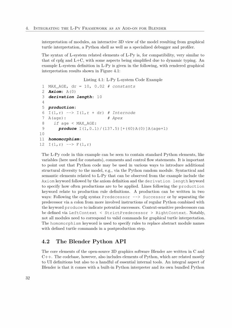
4. Integrating the L-Py Framework as an Add-on for Blender

interpretation of modules, an interactive 3D view of the model resulting from graphicalturtle interpretation, a Python shell as well as a specialized debugger and profiler.

The syntax of L-system related elements of L-Py is, for compatibility, very similar tothat of cpfg and L+C, with some aspects being simplified due to dynamic typing. Anexample L-system definition in L-Py is given in the following, with rendered graphicalinterpretation results shown in Figure 4.1:

Listing 4.1: L-Py L-system Code Example1 MAX_AGE, dr = 10, 0.02 # constants2 Axiom: A(0)3 derivation length: 1045 production:6 I(l,r) --> I(l,r + dr) # Internode7 A(age): # Apex8 if age < MAX_AGE:9 produce I(1,0.1)/(137.5)[+(40)A(0)]A(age+1)1011 homomorphism:12 I(l,r) --> F(l,r)

The L-Py code in this example can be seen to contain standard Python elements, likevariables (here used for constants), comments and control flow statements. It is importantto point out that Python code may be used in various ways to introduce additionalstructural diversity to the model, e.g., via the Python random module. Syntactical andsemantic elements related to L-Py that can be observed from the example include theAxiom keyword followed by the axiom definition and the derivation length keywordto specify how often productions are to be applied. Lines following the productionkeyword relate to production rule definitions. A production can be written in twoways: Following the cpfg syntax Predecessor --> Successor or by separating thepredecessor via a colon from more involved instructions of regular Python combined withthe keyword produce to indicate potential successors. Context-sensitive predecessors canbe defined via LeftContext < StrictPredecessor > RightContext. Notably,not all modules need to correspond to valid commands for graphical turtle interpretation.The homomorphism keyword is used to specify rules to replace abstract module nameswith defined turtle commands in a postproduction step.

4.2 The Blender Python APIThe core elements of the open-source 3D graphics software Blender are written in C andC++. The codebase, however, also includes elements of Python, which are related mostlyto UI definitions but also to a handful of essential internal tools. An integral aspect ofBlender is that it comes with a built-in Python interpreter and its own bundled Python

32

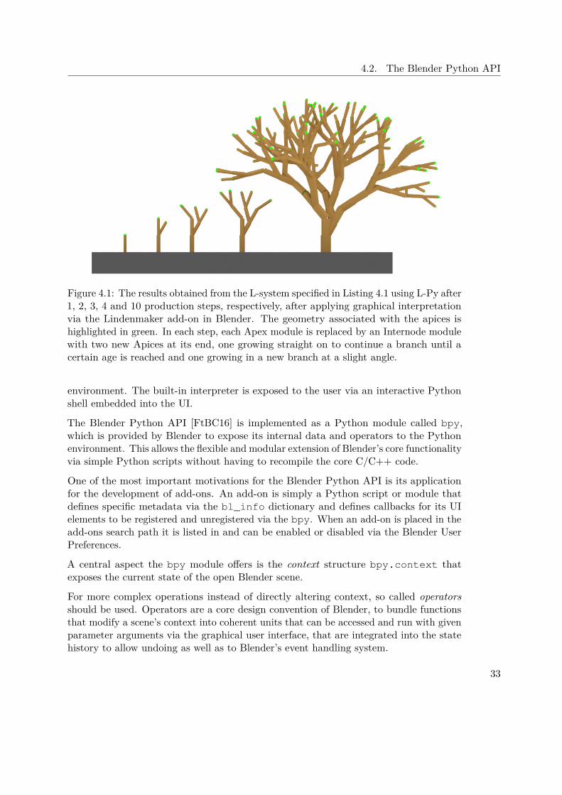
4.2. The Blender Python API

Figure 4.1: The results obtained from the L-system specified in Listing 4.1 using L-Py after1, 2, 3, 4 and 10 production steps, respectively, after applying graphical interpretationvia the Lindenmaker add-on in Blender. The geometry associated with the apices ishighlighted in green. In each step, each Apex module is replaced by an Internode modulewith two new Apices at its end, one growing straight on to continue a branch until acertain age is reached and one growing in a new branch at a slight angle.

environment. The built-in interpreter is exposed to the user via an interactive Pythonshell embedded into the UI.

The Blender Python API [FtBC16] is implemented as a Python module called bpy,which is provided by Blender to expose its internal data and operators to the Pythonenvironment. This allows the flexible and modular extension of Blender’s core functionalityvia simple Python scripts without having to recompile the core C/C++ code.

One of the most important motivations for the Blender Python API is its applicationfor the development of add-ons. An add-on is simply a Python script or module thatdefines specific metadata via the bl_info dictionary and defines callbacks for its UIelements to be registered and unregistered via the bpy. When an add-on is placed in theadd-ons search path it is listed in and can be enabled or disabled via the Blender UserPreferences.

A central aspect the bpy module offers is the context structure bpy.context thatexposes the current state of the open Blender scene.

For more complex operations instead of directly altering context, so called operatorsshould be used. Operators are a core design convention of Blender, to bundle functionsthat modify a scene’s context into coherent units that can be accessed and run with givenparameter arguments via the graphical user interface, that are integrated into the statehistory to allow undoing as well as to Blender’s event handling system.

33

4. Integrating the L-Py Framework as an Add-on for Blender

Among many other things, the API also exposes the creation of custom panels in theBlender user interface, to graphically represent a diversity of input elements that maydirectly expose properties of the scene context among others to be modified by the uservia these UI elements.

For more detailed documentation refer to the official Blender API documentationpages [FtBC16].

4.3 Lindenmaker: A Small Add-on for L-systems inBlender via L-Py

4.3.1 Implementation Considerations

The first step in the development of the Lindenmaker add-on for Blender was to considerhow existing software could be reused to avoid reinventing the wheel. L-Py was developedwith this in mind and is available under an open-source license.

Not all parts of L-Py would be fit for reuse however. Lindenmaker thus aims to form alight wrapping layer around L-Py and uses it as a Python module for the productionof parametric, context-sensitive L-strings. Notably the framework allows to express farmore than these two aspects: stochastic L-systems, for example, can be implementedsimply by using the Python random module within the L-system definition code.

Aspects related to graphical turtle interpretation had to be rewritten from the groundup for Blender via the Blender Python API, thus not relying on the PlantGL frameworkused by L-Py for turtle interpretation.

This section gives an overview over the implementation steps and design decisions involvedin the Lindenmaker add-on. These steps can roughly be outlined as follows:

• Adapt L-Py to be usable in the Blender Python interpreter, and thus by theLindenmaker add-on

• Implement graphical turtle interpretation tailored specifically for environmentalinteraction with a Blender scene, using the Blender Python API.

Adapting L-Py for use as a Python Module in Lindenmaker

An important design consideration was the question of whether it would be possibleto use an L-system production framework built entirely in Python, to avoid any needfor compilation, relying only on code directly interpreted by Python. This would beadvantageous especially for ease of use and installation, requiring only the placement ofthe Python module into the respective Blender add-ons directory, as well as for ease ofmaintenance. However, since L-Py is written in C++ and only uses a Python wrappervia Boost.Python, it still requires compilation. It was considered to completely rewritethe L-Py L-system production framework in Python based on the existing open-source

34

4.3. Lindenmaker: A Small Add-on for L-systems in Blender via L-Py

C++ code, but this was deemed unrealistic given that L-Py consists of over 18000 lines ofcode. Notably, run-time performance of an entirely interpreted production system wouldlikely be significantly worse compared to the compiled C++ code via the Boost.Pythonwrapper.

Using the existing C++ and Boost.Python wrapper code of L-py as an L-system produc-tion framework, it soon became evident that a number of adaptations would be required.Most notably, the Boost.Python aspects of L-Py were written for Python 2.x as a target,but Blender has migrated to Python 3 with version 2.5 and has since dropped supportfor Python 2 [FtBC09]. Moreover, being part of the OpenAlea suite, L-Py relied on abuild process involving custom build tools that would first have to be build themselves inorder to build L-Py and PlantGL. Noting that the last substantial changes to the L-Pycode base date several years back [dReIeeA16b], the decision was taken to avoid tryingto maintain compatibility with the original L-Py source, and build a custom version forPython 3.5 with dependencies to PlantGL removed (the two frameworks as mentionedbeing rather strongly coupled) and using the well documented and widely supportedCMake for the build process.

To get an idea on which parts of L-Py would need adaptation, especially regarding theremoval of dependencies to unused libraries such as to PlantGL for graphical interpretationcode, the first step was to get an overview over the L-Py code base and study its structure.While the code is very clearly structured, there is an evident lack of documentation in thecode itself but more importantly also of the L-Py API on the web [dReIeeA16a]. However,it is still possible to identify parts dependent on the PlantGL library via extensive useof text search tools like grep and inspecting relevant header files. Most dependencieson PlantGL can be removed via simple #ifdef C++ preprocessor directives. Some ofthe more general PlantGL code that L-Py heavily relies on (like utility math structuresand functions) had to be integrated into the L-Py core, given that compatibility to theoriginal L-Py is not a requirement as mentioned before.

Regarding adaptions of the Boost.Python wrapper for Python 3, #ifdef preprocessordirectives were used to conditionally select statements depending on whether Python2 or Python 3 libraries were being used. The differences in Python versions are mostlysubtle changes in function names which can be hard to find without using tools to inspectsymbol references in the resulting object files [Fou09]. L-Py adaptation also raised anumber of other minor issues, such as the use of double underscore names in the L-Pycode, which for the GNU C++ compiler are typically only allowed for reserved names.

Using L-Py as a Python Module in the Blender Python Interpreter

Once the L-Py Python module is built as a shared library (.so on UNIX or .dll onWindows) it can be readily imported to be used by the Python interpreter. Usage ofL-Py is very straightforward. After importing the module via import lpy an Lsystemobject can be created from a source .lpy L-system definition file via a simple commandlsystem = lpy.Lsystem("/path/to/lpyfile.lpy").

35

4. Integrating the L-Py Framework as an Add-on for Blender

A call to lsystem.derive() will trigger the application of production rules to theaxiom for the specified number of derivation steps and return the result in the internalAxialTree representation, which can be converted directly to a string to yield theresulting L-string. The member function lsystem.interpret() can be used to applyhomomorphism substitution rules.

To use the L-Py module in Blender’s Python interpreter, it should be placed within itssearch path [FtBC17a]. This is required for the Lindenmaker add-on to make use of theL-Py framework for L-system productions directly within Blender.

Implementing Turtle Interpretation via the Blender Python API

To provide graphical turtle interpretation in Blender, all functionality related to thisaspect of the Lindenmaker add-on relies on the Blender Python API, instead of thePlantGL library originally used by L-Py.

The central components for drawing, i.e. placement of 3D geometry in this context, areformed by a Python class called Turtle and a subtype of it called DrawingTurtle.

class Turtle:• stores turtle transformation matrix• implements movement and branching turtle commands• allows branching hierarchy to be inspected via Blender scene manager

The Turtle class implements basic turtle interpretation commands related to movement,i.e., translation, rotation, look at, as well as branching. The state of the turtle relating toits orientation in space is stored via a single 4D matrix, which is manipulated for movementvia multiplications with basic transformation matrices. Branching is implemented via astack data structure to which turtle states can be pushed to on branch initialization aswell as retrieved from on branch termination. This turtle is used where draw commandsare not necessary. It can create a branching hierarchy tree of objects, which only storetransformation information, but have no mesh information associated with them thatcould be visualized via rendering and rasterization. The root of this hierarchy tree isformed by an object labeled “Root” in the Blender scene. The hierarchy of objectsproduced is managed via the Blender object parenting system, and can thus be inspectedand modified in the Blender scene after graphical interpretation.

class DrawingTurtle:• stores turtle state and configuration related to drawing• implements turtle drawing commands using 3D mesh instances

The DrawingTurtle subtype extends the simple turtle by providing various methodsimplementing the draw commands related to graphical interpretation. Its state isextended by a number of fields related to drawing, such as internode width and lengthas well as material index. Drawing in terms of the Blender Python API module bpycorresponds to the creation of 3D objects with the current turtle matrix state thatalso include mesh information. For the standard draw command F, which is used

36

4.3. Lindenmaker: A Small Add-on for L-systems in Blender via L-Py

to draw an internode of a plant structure, instances of a predefined simple cylindermesh named “LindenmakerDefaultInternodeMesh” are created, which all share thesame mesh data to avoid redundancy. If desired, another predefined mesh named“LindenmakerDefaultNodeMesh” can also be used to draw simple spheres to indicatebranching points. Both meshes can be customized or replaced entirely – the same beingthe case for colors and materials used for rendering – as described in the following UserInterface Overview subsection. Additionally, objects associated with instances of a custommesh defined in the Blender scene can be generated in the current turtle matrix state viathe ~ command, which will be discussed in more detail in Section 4.4.

function turtle_interpretation.interpret():• parses L-string produced by L-Py• splits L-string into individual commands with associated parameters• forwards commands to Turtle member functions• applies branch cut commands

The turtle classes just described interface closely with the bpy module, but are in-dependent of the L-Py library. Calls to the turtle are done mostly by the functionturtle_interpretation.interpret(), which parses a simple input string repre-senting the L-string produced by L-Py or any other L-system production framework, andinterprets it graphically according to drawing parameters specified by the user via theLindenmaker UI. This function uses Python’s regular expression functionality to splitthe L-string into the individual interpretation commands together with their associatedparameters contained in parentheses, and calls the respective Turtle methods for validcommands and parameter values. Additionally, it applies the cut branch command % onthe L-string level before turtle interpretation. This is done by removing all commandsymbols following the cut command symbol until the end of the branch, i.e., until thenext unmatched closing bracket or the end of the string.

class LindenmakerPanel:• provides main Lindenmaker user interface

The interface of Lindenmaker to the user is implemented via the LindenmakerPanelclass. This is a subtype of bpy.types.Panel, which is one of the main ways ofspecifying UI elements through the Blender Python API. The user interface will bedescribed in more detail in the following subsection.

class LindenmakerOperator:• used to embed Lindenmaker functionality into the Blender event handling system• required to provide undo/redo capabilities

Buttons specified by the LindenmakerPanel are used to evoke methods of anotherclass named LindenmakerOperator. This is a subtype of bpy.types.Operator,which, as previously described, is a central aspect of the Blender Python API to achievemodularity. Essentially, it is used to integrate custom functionality that change a Blenderscene’s state into the state history to allow undoing as well as to Blender’s event handlingsystem in a unified way. The LindenmakerOperator not only makes calls to the

37

4. Integrating the L-Py Framework as an Add-on for Blender

turtle_interpretation.interpret() function, but also interfaces with the L-Pylibrary module. It takes the input .lpy L-system specification file and calls the L-Pylsystem.derive() method to apply a given number of production steps accordingto production rules to the current L-string, and then calls lsystem.interpret() toapply L-string substitutions according to homomorphism rules specified in the .lpyfile. The latter function, however, does not do any graphical turtle interpretation. Itis used only to translate abstract L-string symbols into actual commands relating tographical turtle interpretation. Graphical interpretation is done as described via thecustom turtle_interpretation.interpret() function provided by Lindenmaker,which should thus not be confused with lsystem.interpret().

4.3.2 User Interface Overview

To use the Lindenmaker add-on, it is installed by being placed in the add-ons searchpath, and enabled from the user preferences panel. When it is enabled, a new tab labeledLindenmaker is apparent in the Tool Shelf panel of the 3D View area, as seen onthe left in Figure 4.2. This is where all UI elements of Lindenmaker reside, which shallbe explained in the following.

[filepath] L-Py File: Path of .lpy file containing L-system definition.

[float] Default Turtle Step Size: Default length value for F (move turtleand draw) and f (move turtle) commands if no arguments given.

[float] Default Rotation Angle: Default angle in degrees for turtle rotationcommands if no argument given.

[mesh] Internode: Name of mesh to be used for drawing internodes via the Fcommand. Default is “LindenmakerDefaultInternodeMesh", a cylinder mesh generated atfirst use.

[float] Default Line Width: Default width of internode and node objects drawnvia F command.

[float] Width Growth Factor: Factor by which line width is multiplied via ;(width increment) command. Also for , (width decrement) command as 1− (factor− 1).

[float] Internode Length Scale: Factor by which move step size is multipliedto yield internode length. Used to allow internode length to deviate from step size.

[checkbox/mesh] Nodes: If enabled, the selected node mesh is drawn at branchingpoints. If not enabled uses Empty objects if hierarchy is used. Default is “Lindenmak-erDefaultNodeMesh", a simple icosphere mesh generated at first use.

[checkbox] Recreate Default Internode / Node Meshes: If enabled, recre-ates “LindenmakerDefaultInternodeMesh” and “LindenmakerDefaultNodeMesh", accord-ing to attribute values specified via the following fields.

[integer] Default Internode Cylinder Vertices: Number of base circlevertices for default cylinder “LindenmakerDefaultInternodeMesh".

38

4.3. Lindenmaker: A Small Add-on for L-systems in Blender via L-Py

[integer] Default Node Icosphere Subdivision: Number of subdivisionsteps for default icosphere “LindenmakerDefaultNodeMesh".

[checkbox] Force Flat Shading: Force flat shading for all parts of the generatedstructure.

[checkbox] Single Object (No Hierarchy, Faster) If enabled, generate asingle object with a single joined mesh. If disabled, generate a branching hierarchy ofobjects. Having this option enabled is significantly faster.

[checkbox] Remove Last Interpretation Result: If enabled, the last objectlabeled “Root” generated from the previous interpretation is replaced. Useful for stepwiseproduction and interpretation, to avoid cluttering the scene.

[button] Add Mesh via Lindenmayer System: Do the whole process from L-system definition to graphical interpretation. Pass .lpy file to L-Py to produce L-string.Apply production rules as many times as specified in file, then apply homomorphismsubstitution rules. Finally create a graphical interpretation of the L-string based on theUI options.

[button] Clear Current L-strings: Clear the currently stored L-strings. Notethat while the L-system yields just one L-string, two copies of the L-string are stored:One used for production and one used for graphical turtle interpretation. See below fordetails.

[button] Apply One Production Step: Apply a single production step to cur-rent L-string, or to the L-system axiom in the first production step. No graphical turtleinterpretation is done.

[textfield] L-string for Production: The produced L-string used for furtherstepwise production. Manual modifications are possible by editing the textfield contentsdirectly, usage of copy/paste to edit externally is however more convenient, as L-stringstend to become very long with increasing number of production steps.

[textfield] Homomorphism (For Interpretation): The same produced L-string but with homomorphism substitution rules applied (if given), used for graphicalturtle interpretation. “Homomorphism” is a L-Py feature intended as a final postproduc-tion step to replace abstract module names with actual interpretation commands. InL-Py these rules are preceded by the keyword homomorphism: or interpretation:(including the colon). Once homomorphisms are applied the L-string can no longer beused for stepwise production, thus two L-strings have to be stored.

[button] Interpret L-string via Turtle Graphics: Interpret current L-string via graphical turtle interpretation. No production steps are applied.

[button] Produce Step and Interpret: Apply a single production step andinterpret.

The result of the graphical interpretation is generated as an object labeled “Root",which is displayed in the central 3D View of the Blender user interface, as seen in

39

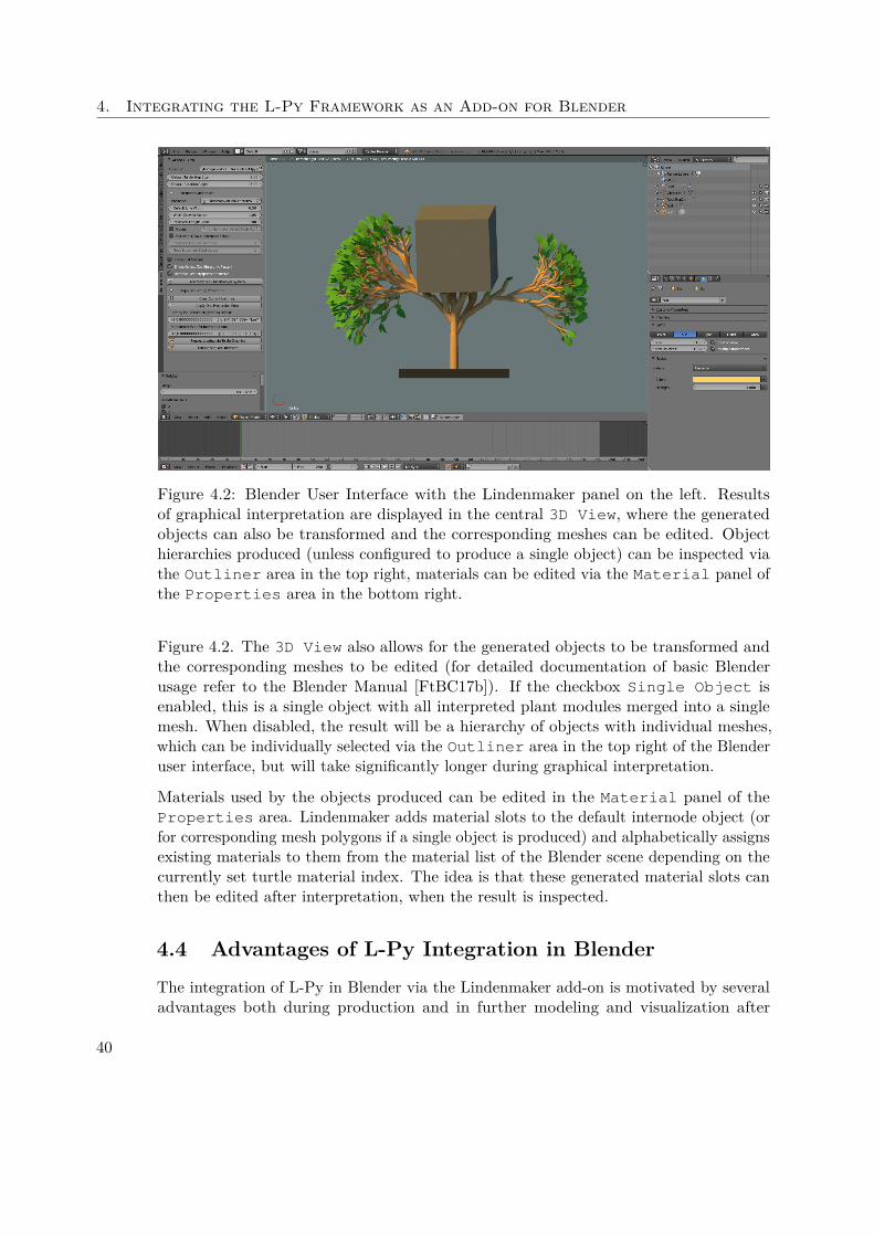
4. Integrating the L-Py Framework as an Add-on for Blender

Figure 4.2: Blender User Interface with the Lindenmaker panel on the left. Resultsof graphical interpretation are displayed in the central 3D View, where the generatedobjects can also be transformed and the corresponding meshes can be edited. Objecthierarchies produced (unless configured to produce a single object) can be inspected viathe Outliner area in the top right, materials can be edited via the Material panel ofthe Properties area in the bottom right.

Figure 4.2. The 3D View also allows for the generated objects to be transformed andthe corresponding meshes to be edited (for detailed documentation of basic Blenderusage refer to the Blender Manual [FtBC17b]). If the checkbox Single Object isenabled, this is a single object with all interpreted plant modules merged into a singlemesh. When disabled, the result will be a hierarchy of objects with individual meshes,which can be individually selected via the Outliner area in the top right of the Blenderuser interface, but will take significantly longer during graphical interpretation.

Materials used by the objects produced can be edited in the Material panel of theProperties area. Lindenmaker adds material slots to the default internode object (orfor corresponding mesh polygons if a single object is produced) and alphabetically assignsexisting materials to them from the material list of the Blender scene depending on thecurrently set turtle material index. The idea is that these generated material slots canthen be edited after interpretation, when the result is inspected.

4.4 Advantages of L-Py Integration in Blender

The integration of L-Py in Blender via the Lindenmaker add-on is motivated by severaladvantages both during production and in further modeling and visualization after

40

4.4. Advantages of L-Py Integration in Blender

production. While examples of the applications of these features are given in the followingchapter, this section shall give a more abstract overview and especially introduce someof the specific new interpretation modules in Lindenmaker that can be used to modelenvironmental interaction.

Some of the advantages in the post-production stage include:

• direct integration with the Blender path-tracing renderer Cycles, allowing for therealistic simulation of light propagation in the modeled structure

• access to modifiers and sculpting tools to further improve a model after production

• possibility to visualize the hierarchy of branches in a growing structure via theBlender parent-child system

• integration with simulation tools like particle system, wind simulation etc., allowingfor example the modeling of a field of flowers

Of greater interest, however, are the possibilities during L-Py production, most notablythe following:

• access to mesh and interpolated curve modeling tools to model custom objects,such as specific parts of a plant, that can be referenced in L-Py production

• interaction with a Blender scene via direct access to Blender structures during L-Pyproduction, together with Lindenmaker turtle state query and look at modules, tomodel environmental interaction

The inclusion of custom-modeled objects is an essential feature of most modern L-systemframeworks. In Lindenmaker, it follows the conventional syntax and is done via theinterpretation module ~, which takes as arguments the referenced object’s name in doublequotes as well as optional scaling factors for uniform scaling or scaling along individuallocal turtle coordinate directions. Examples would be ~("Flower"), ~("Flower",0.5) and ~("Flower", 0.2, 0.3, 0.4).

The most notable advantage of the integration with Blender is that it allows an interactionof the growing structure with its environment similar to the approach of open L-systemsdiscussed in Section 3.6.3. This interaction is facilitated by the fact that the BlenderPython API, being based on Python just like L-Py, may be used to access informationabout the currently open Blender scene directly during production. This is achieved byimporting the bpy module directly in the L-Py code via import bpy, allowing accessto bpy.context.scene and similar structures. Without Blender integration, it isnot straightforward to integrate production rules into an environment as complex as aBlender scene.

41

4. Integrating the L-Py Framework as an Add-on for Blender

To use the current state of the turtle to influence production, Lindenmaker in anal-ogy to the original L-Py offers a query command ?. This command can be usedto query any of the turtle matrix column vectors (heading, left, up, position) via?("H"|"L"|"U"|"P",0,0,0), e.g. for the turtle position vector ?("P",0,0,0).The three zeros 0,0,0 are placeholders that will be replaced by the queried vector x,y,zvalues. To use the queried values, a production rule for the ? module should be added,as demonstrated by the following example:

Listing 4.2: Lindenmaker Query Module Example1 production:2 A: # Apex3 produce ?("P",0,0,0)I/(137.5)

?("P",0,0,0)[+(40)?("P",0,0,0)A]A45 ?(vector,x,y,z):6 if vector == "P":7 print("turtle position: {} {} {}".format(x,y,z))8 if y > 5:9 produce ~("Flower")

In this rather arbitrary example, multiple query modules are inserted by the Apexmodule. Lindenmaker will replace the 0,0,0 placeholders with the actual x,y,z valuesof the queried vectors. The production rule for the query module can then be used toreplace the query module with something else, depending on the vector values which aregiven as parameter arguments. Here, positional queries are replaced by a flower objectif the y value of the position vector is bigger than 5. By comparing the turtle state toother variables from bpy.context.scene, this allows the modeling of environmentalinteraction of plants with a Blender scene.

Another new turtle interpretation command added in Lindenmaker is the look at command@(x, y, z). This command will reorient the turtle so that the heading vector ispointing toward the given target position x, y, z, while the heading, left and up vectorsare guaranteed to have the same relative orientation (handedness) as before. This can beused together with Blender scene information via the bpy module, to orient a growingstructure toward an object, e.g. toward a light source to simulate phototropism. ThePython random module can be used to add random deviation from the look at direction.

It is important to note that some of the customizations necessary to adapt L-Py toBlender mean that some of the original L-Py interpretation modules can not be used viathe Lindenmaker add-on, and vice-versa. This partial break of compatibility is howeverdeemed acceptable since L-Py appears to be no longer actively maintained [dReIeeA16c].

42

CHAPTER 5Modeling Plant Structures via

L-systems in Blender

This chapter will show some examples of what can be achieved using the Lindenmakeradd-on to integrate L-Py L-system production in Blender.

First, some results of the graphical interpretation via the Lindenmaker add-on will begiven, focusing on well-known L-system models of plant inflorescence. Moreover, some ofthe advantages of having the full feature set of a 3D computer graphics suite like Blenderat hand are shown, such as the use of particle systems and simulation tools, e.g., tomodel a field of flowers. All results will be rendered directly in Blender using the Cyclespath tracer, which is also a notable advantage of this integration.

More detailed consideration, however, is given to another main advantage of Blenderintegration for L-system production. It is important to note that this integration notonly enables the direct graphical interpretation, i.e., the creation of 3D meshes, in awidely used modeling tool: It also means that L-System production code, being based onPython, can have access to the whole context of a Blender scene via the Blender PythonAPI. Having access to the structures of a Blender scene during production is very usefulto model environmental interaction. Special attention will thus be given to this aspect,which is one of the main motivations to integrate L-system production into a generalpurpose modeling tool like Blender.

5.1 Modeling Herbaceous Plants and Inflorescence

5.1.1 Mycelis muralis

One of the more well-known examples of an L-system used to model plant inflorescence isthat of Mycelis muralis (wall letuce), introduced by Janssen and Lindenmayer [JL87] and

43

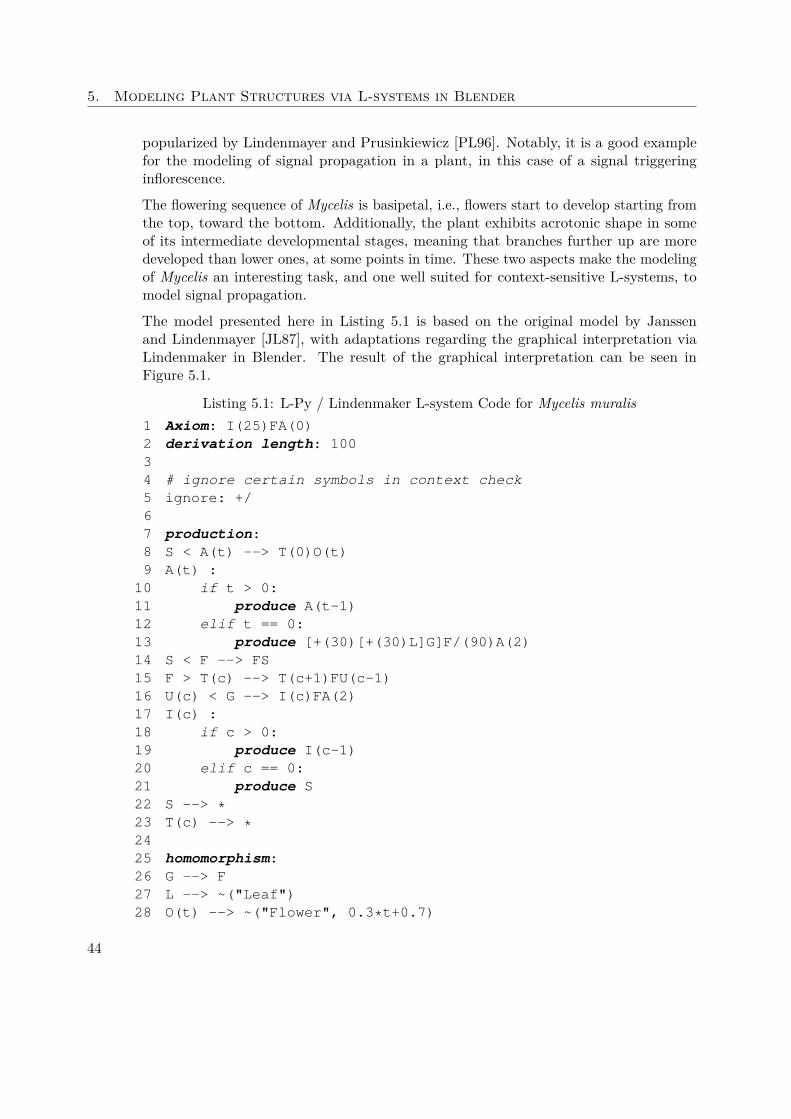
5. Modeling Plant Structures via L-systems in Blender

popularized by Lindenmayer and Prusinkiewicz [PL96]. Notably, it is a good examplefor the modeling of signal propagation in a plant, in this case of a signal triggeringinflorescence.

The flowering sequence of Mycelis is basipetal, i.e., flowers start to develop starting fromthe top, toward the bottom. Additionally, the plant exhibits acrotonic shape in someof its intermediate developmental stages, meaning that branches further up are moredeveloped than lower ones, at some points in time. These two aspects make the modelingof Mycelis an interesting task, and one well suited for context-sensitive L-systems, tomodel signal propagation.

The model presented here in Listing 5.1 is based on the original model by Janssenand Lindenmayer [JL87], with adaptations regarding the graphical interpretation viaLindenmaker in Blender. The result of the graphical interpretation can be seen inFigure 5.1.

Listing 5.1: L-Py / Lindenmaker L-system Code for Mycelis muralis1 Axiom: I(25)FA(0)2 derivation length: 10034 # ignore certain symbols in context check5 ignore: +/67 production:8 S < A(t) --> T(0)O(t)9 A(t) :10 if t > 0:11 produce A(t-1)12 elif t == 0:13 produce [+(30)[+(30)L]G]F/(90)A(2)14 S < F --> FS15 F > T(c) --> T(c+1)FU(c-1)16 U(c) < G --> I(c)FA(2)17 I(c) :18 if c > 0:19 produce I(c-1)20 elif c == 0:21 produce S22 S --> *23 T(c) --> *2425 homomorphism:26 G --> F27 L --> ~("Leaf")28 O(t) --> ~("Flower", 0.3*t+0.7)

44

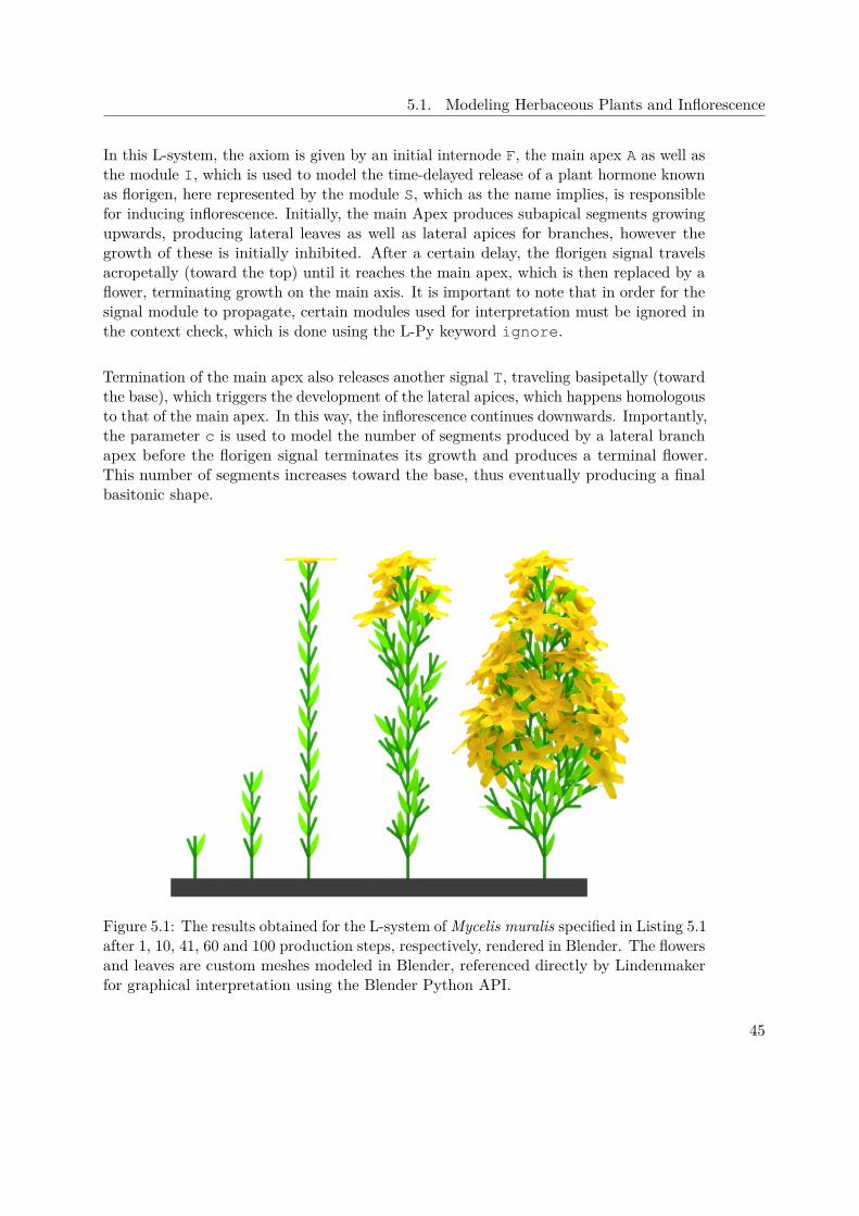
5.1. Modeling Herbaceous Plants and Inflorescence

In this L-system, the axiom is given by an initial internode F, the main apex A as well asthe module I, which is used to model the time-delayed release of a plant hormone knownas florigen, here represented by the module S, which as the name implies, is responsiblefor inducing inflorescence. Initially, the main Apex produces subapical segments growingupwards, producing lateral leaves as well as lateral apices for branches, however thegrowth of these is initially inhibited. After a certain delay, the florigen signal travelsacropetally (toward the top) until it reaches the main apex, which is then replaced by aflower, terminating growth on the main axis. It is important to note that in order for thesignal module to propagate, certain modules used for interpretation must be ignored inthe context check, which is done using the L-Py keyword ignore.

Termination of the main apex also releases another signal T, traveling basipetally (towardthe base), which triggers the development of the lateral apices, which happens homologousto that of the main apex. In this way, the inflorescence continues downwards. Importantly,the parameter c is used to model the number of segments produced by a lateral branchapex before the florigen signal terminates its growth and produces a terminal flower.This number of segments increases toward the base, thus eventually producing a finalbasitonic shape.

Figure 5.1: The results obtained for the L-system of Mycelis muralis specified in Listing 5.1after 1, 10, 41, 60 and 100 production steps, respectively, rendered in Blender. The flowersand leaves are custom meshes modeled in Blender, referenced directly by Lindenmakerfor graphical interpretation using the Blender Python API.

45

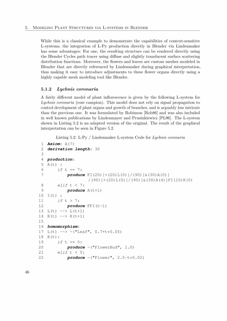
5. Modeling Plant Structures via L-systems in Blender

While this is a classical example to demonstrate the capabilities of context-sensitiveL-systems, the integration of L-Py production directly in Blender via Lindenmakerhas some advantages: For one, the resulting structure can be rendered directly usingthe Blender Cycles path tracer using diffuse and slightly translucent surface scatteringdistribution functions. Moreover, the flowers and leaves are custom meshes modeled inBlender that are directly referenced by Lindenmaker during graphical interpretation,thus making it easy to introduce adjustments to these flower organs directly using ahighly capable mesh modeling tool like Blender.

5.1.2 Lychnis coronaria

A fairly different model of plant inflorescence is given by the following L-system forLychnis coronaria (rose campion). This model does not rely on signal propagation tocontrol development of plant organs and growth of branches, and is arguably less intricatethan the previous one. It was formulated by Robinson [Rob86] and was also includedin well known publications by Lindenmayer and Prusinkiewicz [PL96]. The L-systemshown in Listing 5.2 is an adapted version of the original. The result of the graphicalinterpretation can be seen in Figure 5.2.

Listing 5.2: L-Py / Lindenmaker L-system Code for Lychnis coronaria1 Axiom: A(7)2 derivation length: 3034 production:5 A(t) :6 if t == 7:7 produce FI(20)[+(20)L(0)]/(90)[&(30)A(0)]

/(90)[+(20)L(0)]/(90)[&(30)A(4)]FI(10)K(0)8 elif t < 7:9 produce A(t+1)10 I(t) :11 if t > 7:12 produce FFI(t-1)13 L(t) --> L(t+1)14 K(t) --> K(t+1)1516 homomorphism:17 L(t) --> ~("Leaf", 0.7+t*0.05)18 K(t):19 if t >= 5:20 produce ~("FlowerBud", 1.0)21 elif t < 5:22 produce ~("Flower", 2.5-t*0.02)

46

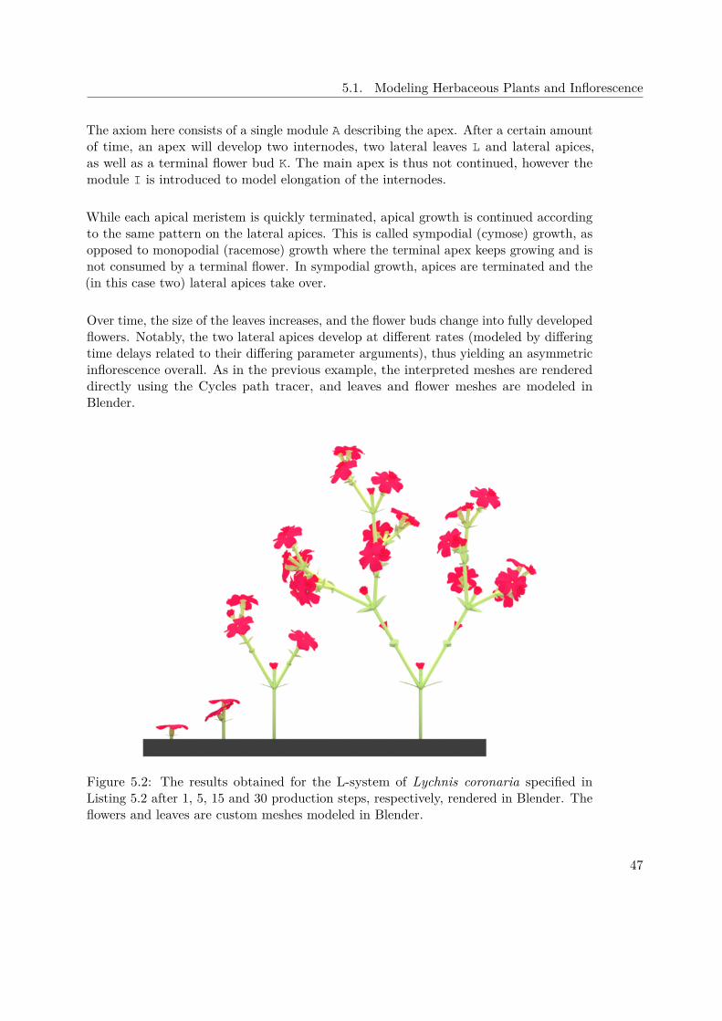
5.1. Modeling Herbaceous Plants and Inflorescence

The axiom here consists of a single module A describing the apex. After a certain amountof time, an apex will develop two internodes, two lateral leaves L and lateral apices,as well as a terminal flower bud K. The main apex is thus not continued, however themodule I is introduced to model elongation of the internodes.

While each apical meristem is quickly terminated, apical growth is continued accordingto the same pattern on the lateral apices. This is called sympodial (cymose) growth, asopposed to monopodial (racemose) growth where the terminal apex keeps growing and isnot consumed by a terminal flower. In sympodial growth, apices are terminated and the(in this case two) lateral apices take over.

Over time, the size of the leaves increases, and the flower buds change into fully developedflowers. Notably, the two lateral apices develop at different rates (modeled by differingtime delays related to their differing parameter arguments), thus yielding an asymmetricinflorescence overall. As in the previous example, the interpreted meshes are rendereddirectly using the Cycles path tracer, and leaves and flower meshes are modeled inBlender.

Figure 5.2: The results obtained for the L-system of Lychnis coronaria specified inListing 5.2 after 1, 5, 15 and 30 production steps, respectively, rendered in Blender. Theflowers and leaves are custom meshes modeled in Blender.

47

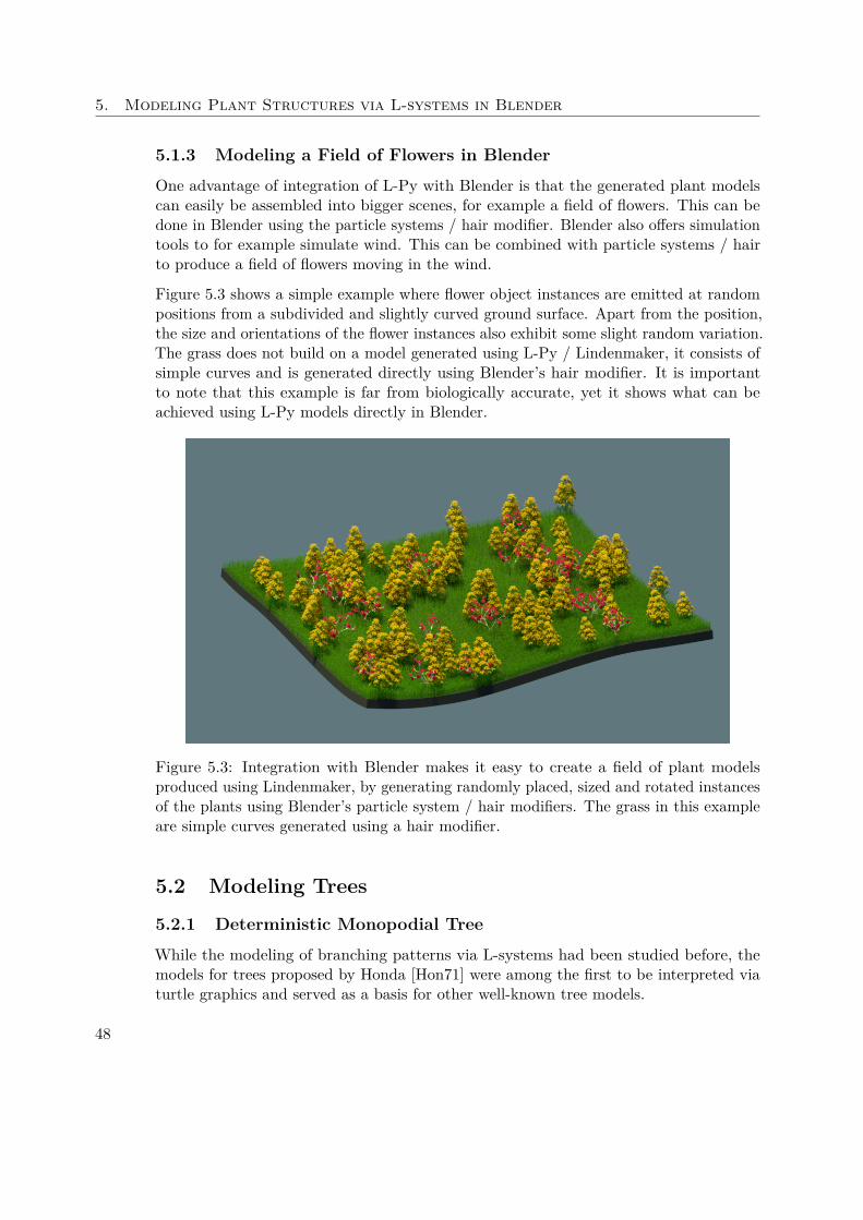
5. Modeling Plant Structures via L-systems in Blender

5.1.3 Modeling a Field of Flowers in Blender

One advantage of integration of L-Py with Blender is that the generated plant modelscan easily be assembled into bigger scenes, for example a field of flowers. This can bedone in Blender using the particle systems / hair modifier. Blender also offers simulationtools to for example simulate wind. This can be combined with particle systems / hairto produce a field of flowers moving in the wind.

Figure 5.3 shows a simple example where flower object instances are emitted at randompositions from a subdivided and slightly curved ground surface. Apart from the position,the size and orientations of the flower instances also exhibit some slight random variation.The grass does not build on a model generated using L-Py / Lindenmaker, it consists ofsimple curves and is generated directly using Blender’s hair modifier. It is importantto note that this example is far from biologically accurate, yet it shows what can beachieved using L-Py models directly in Blender.

Figure 5.3: Integration with Blender makes it easy to create a field of plant modelsproduced using Lindenmaker, by generating randomly placed, sized and rotated instancesof the plants using Blender’s particle system / hair modifiers. The grass in this exampleare simple curves generated using a hair modifier.

5.2 Modeling Trees

5.2.1 Deterministic Monopodial Tree

While the modeling of branching patterns via L-systems had been studied before, themodels for trees proposed by Honda [Hon71] were among the first to be interpreted viaturtle graphics and served as a basis for other well-known tree models.

48

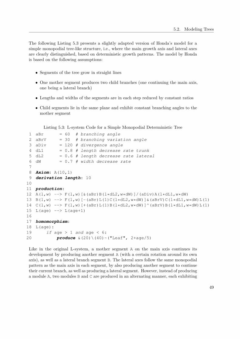
5.2. Modeling Trees

The following Listing 5.3 presents a slightly adapted version of Honda’s model for asimple monopodial tree-like structure, i.e., where the main growth axis and lateral axesare clearly distinguished, based on deterministic growth patterns. The model by Hondais based on the following assumptions:

• Segments of the tree grow in straight lines

• One mother segment produces two child branches (one continuing the main axis,one being a lateral branch)

• Lengths and widths of the segments are in each step reduced by constant ratios

• Child segments lie in the same plane and exhibit constant branching angles to themother segment

Listing 5.3: L-system Code for a Simple Monopodial Deterministic Tree1 aBr = 60 # branching angle2 aBrV = 30 # branching variation angle3 aDiv = 120 # divergence angle4 dL1 = 0.8 # length decrease rate trunk5 dL2 = 0.6 # length decrease rate lateral6 dW = 0.7 # width decrease rate78 Axiom: A(10,1)9 derivation length: 101011 production:12 A(l,w) --> F(l,w)[&(aBr)B(l*dL2,w*dW)]/(aDiv)A(l*dL1,w*dW)13 B(l,w) --> F(l,w)[-(aBr)L(1)C(l*dL2,w*dW)]&(aBrV)C(l*dL1,w*dW)L(1)14 C(l,w) --> F(l,w)[+(aBr)L(1)B(l*dL2,w*dW)]^(aBrV)B(l*dL1,w*dW)L(1)15 L(age) --> L(age+1)1617 homomorphism:18 L(age):19 if age > 1 and age < 6:20 produce &(20)\(40)~("Leaf", 2+age/5)

Like in the original L-system, a mother segment A on the main axis continues itsdevelopment by producing another segment A (with a certain rotation around its ownaxis), as well as a lateral branch segment B. The lateral axes follow the same monopodialpattern as the main axis in each segment, by also producing another segment to continuetheir current branch, as well as producing a lateral segment. However, instead of producinga module A, two modules B and C are produced in an alternating manner, each exhibiting

49

5. Modeling Plant Structures via L-systems in Blender

slightly different branching angles. The length and width for newly produced segmentsdecreases by a constant multiplicative factor in each step.

In the adapted version here, branching angles are customized such that main and lateralsegments do not lie in the same plane, but rather exhibit some variation. Also, simpleleaves have been added growing at the outermost branches, which change size slightlydepending on their age. Results of the graphical interpretation can be seen in Figure 5.4.

Figure 5.4: The results obtained for the adapted L-system specified in Listing 5.3 of amonopodial tree-like structure based on Honda [Hon71] after 1, 2, 3, 6 and 10 steps.

5.2.2 Randomized Tree with Stochastic Branch Termination

The previous tree model was characterized by deterministic production rules. Morerealistic and aesthetically pleasing results can be achieved by introducing randomness inthe patterns of growth, to better simulate the many factors influencing growth that cannot be included directly in the model. Since L-Py and Lindenmaker are based on Python,this can be achieved by using the Python random module directly in the L-systemproduction code.

The following model in Listing 5.4 is based on a model presented by Lindenmayer andPrusinkiewicz [PL96], which however exhibits deterministic production rules. In order toadd randomness in the growth patterns, the model presented here is thus a somewhatmodified version that does not resemble the original too much.

Listing 5.4: L-system Code for a Tree with Randomized Tertiary Branching Characteristicsand Stochastic Branch Termination1 import random23 aDiv1 = 95 # divergence angle 14 aDiv2 = 133 # divergence angle 2

50

5.2. Modeling Trees

5 aBr = 25 # branching angle6 dL = 1.05 # elongation rate7 dW = 1.2 # width increase rate8 maxApexAge = 3 # age as branch stops terminal growth9 leafStartTime = 2 # time as leaves start to grow1011 Axiom: I(3,0.3)/(45)A(0,0)12 derivation length: 51314 production:15 I(l,w): # Internode16 rnd = random.random()/4+117 produce I(l*dL*rnd, w*dW)18 L(age, t) --> L(age+1, t) # Leaf19 A(age, t): # Apex20 rnd = random.random()/2+0.7521 if age <= maxApexAge and rnd > 0.9:22 produce I(1,0.3)

[&(aBr*rnd)I(1,0.3)L(0,t+1)A(0,t+1)]I(0.5,0.3)/(aDiv1*rnd)[&(aBr*rnd)I(1,0.3)L(0,t+1)A(0,t+1)]/(aDiv2*rnd)[I(1,0.3)A(age+1,t+1)]

2324 homomorphism:25 I(l,w) --> F(l,w)26 L(age, t):27 if t > leafStartTime and age < 3:28 produce ~("Leaf", 1.5+age/5)

An apex module A forms the basis of production, each producing three child branchesat differing angles, thus exhibiting ternary branching characteristics. Each child branchalso has its own apex that continues growth in the same manner as the parent branch.In this modified model, slight random variation has been added to branching angles.

Like in the original model, this model differs from the previous tree-like model inListing 5.3 in that branch segments are not treated as static dead matter, but ratheras evolving parts of a growing structure. Therefore, segments are represented by aninternode module I that also changes its length and width dynamically over time, insteadof just having internodes produced at different scale in their initial production. Here, thechange in length is also varied via a random factor.

The most drastic difference to the original model in terms of random variation here is thata random factor is checked against a fixed value to determine with a given probabilitywhether a branch should be terminated. This is essential to add to the plausibility ofthe resulting structure, especially for large scale structures like trees that are heavilyinfluenced by external factors and where fully deterministic unfolding of fixed patterns

51

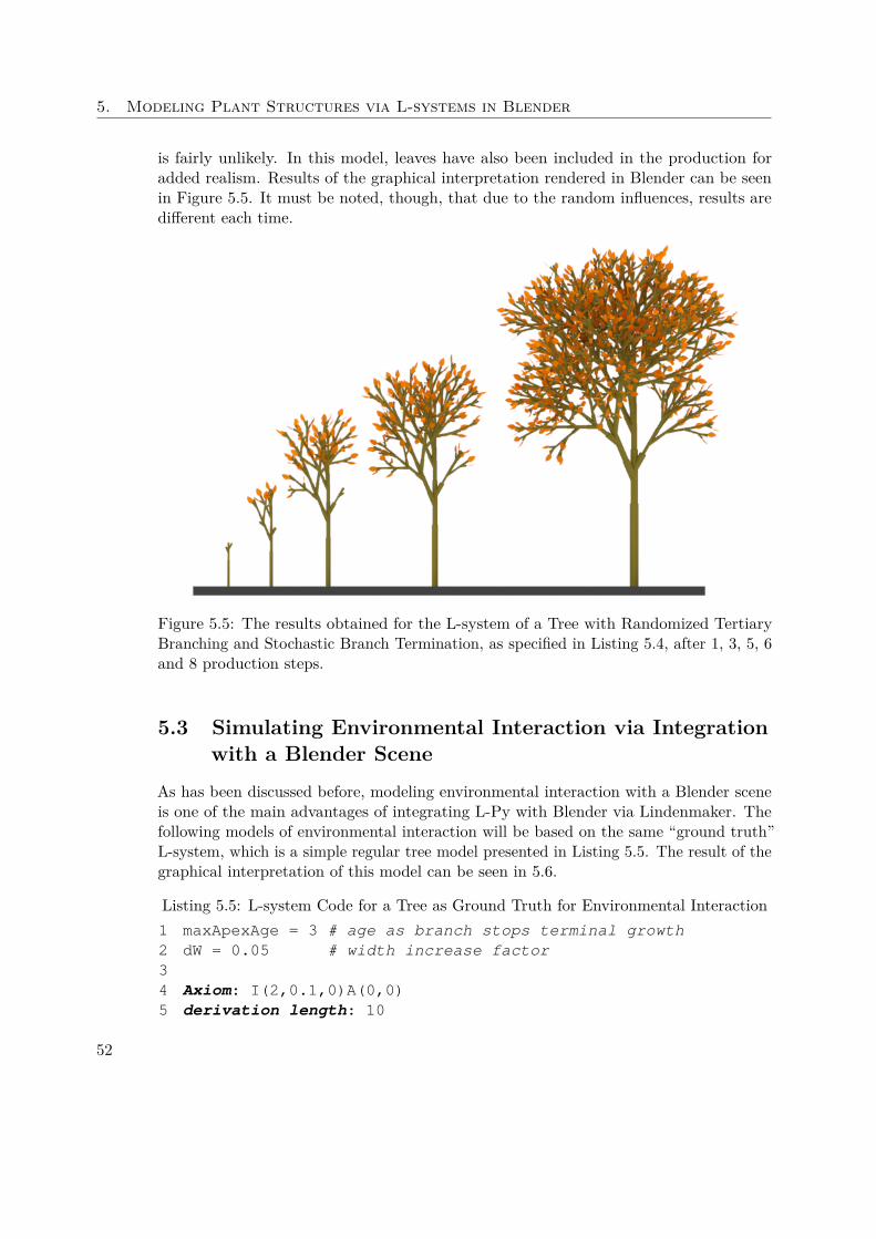
5. Modeling Plant Structures via L-systems in Blender

is fairly unlikely. In this model, leaves have also been included in the production foradded realism. Results of the graphical interpretation rendered in Blender can be seenin Figure 5.5. It must be noted, though, that due to the random influences, results aredifferent each time.

Figure 5.5: The results obtained for the L-system of a Tree with Randomized TertiaryBranching and Stochastic Branch Termination, as specified in Listing 5.4, after 1, 3, 5, 6and 8 production steps.

5.3 Simulating Environmental Interaction via Integrationwith a Blender Scene

As has been discussed before, modeling environmental interaction with a Blender sceneis one of the main advantages of integrating L-Py with Blender via Lindenmaker. Thefollowing models of environmental interaction will be based on the same “ground truth”L-system, which is a simple regular tree model presented in Listing 5.5. The result of thegraphical interpretation of this model can be seen in 5.6.

Listing 5.5: L-system Code for a Tree as Ground Truth for Environmental Interaction1 maxApexAge = 3 # age as branch stops terminal growth2 dW = 0.05 # width increase factor34 Axiom: I(2,0.1,0)A(0,0)5 derivation length: 10

52

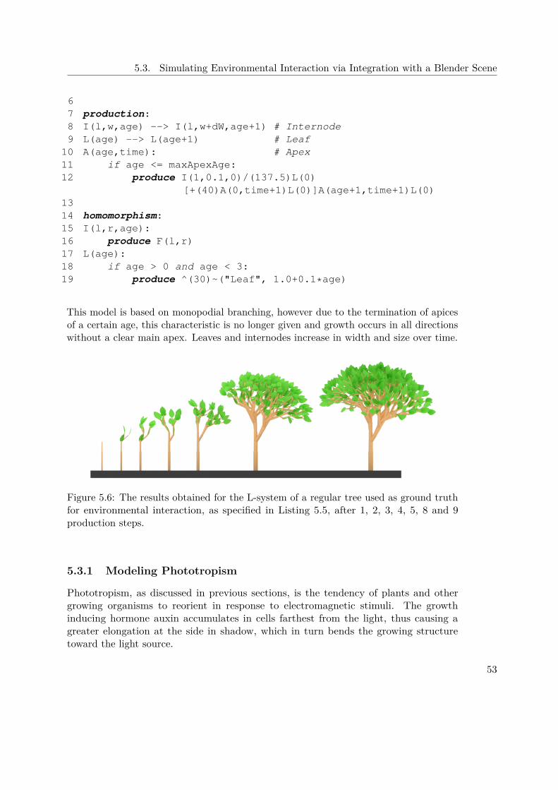
5.3. Simulating Environmental Interaction via Integration with a Blender Scene

67 production:8 I(l,w,age) --> I(l,w+dW,age+1) # Internode9 L(age) --> L(age+1) # Leaf10 A(age,time): # Apex11 if age <= maxApexAge:12 produce I(1,0.1,0)/(137.5)L(0)

[+(40)A(0,time+1)L(0)]A(age+1,time+1)L(0)1314 homomorphism:15 I(l,r,age):16 produce F(l,r)17 L(age):18 if age > 0 and age < 3:19 produce ^(30)~("Leaf", 1.0+0.1*age)

This model is based on monopodial branching, however due to the termination of apicesof a certain age, this characteristic is no longer given and growth occurs in all directionswithout a clear main apex. Leaves and internodes increase in width and size over time.

Figure 5.6: The results obtained for the L-system of a regular tree used as ground truthfor environmental interaction, as specified in Listing 5.5, after 1, 2, 3, 4, 5, 8 and 9production steps.

5.3.1 Modeling Phototropism

Phototropism, as discussed in previous sections, is the tendency of plants and othergrowing organisms to reorient in response to electromagnetic stimuli. The growthinducing hormone auxin accumulates in cells farthest from the light, thus causing agreater elongation at the side in shadow, which in turn bends the growing structuretoward the light source.

53

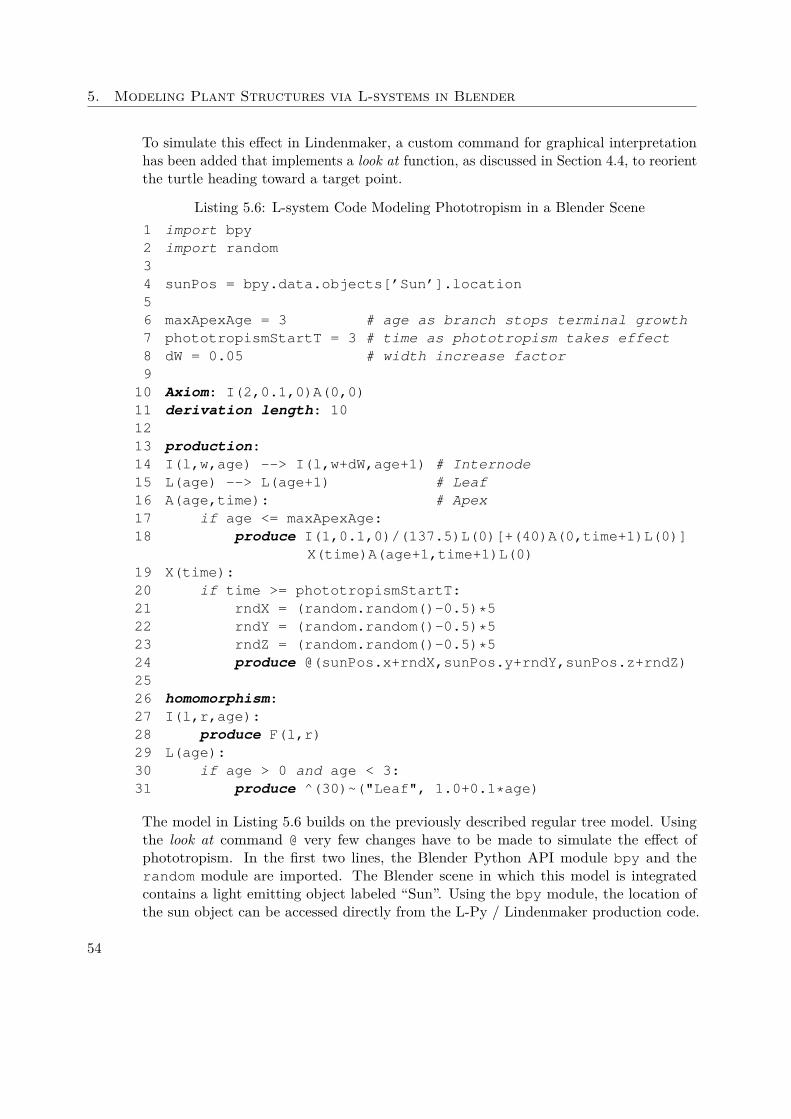
5. Modeling Plant Structures via L-systems in Blender

To simulate this effect in Lindenmaker, a custom command for graphical interpretationhas been added that implements a look at function, as discussed in Section 4.4, to reorientthe turtle heading toward a target point.

Listing 5.6: L-system Code Modeling Phototropism in a Blender Scene1 import bpy2 import random34 sunPos = bpy.data.objects[’Sun’].location56 maxApexAge = 3 # age as branch stops terminal growth7 phototropismStartT = 3 # time as phototropism takes effect8 dW = 0.05 # width increase factor910 Axiom: I(2,0.1,0)A(0,0)11 derivation length: 101213 production:14 I(l,w,age) --> I(l,w+dW,age+1) # Internode15 L(age) --> L(age+1) # Leaf16 A(age,time): # Apex17 if age <= maxApexAge:18 produce I(1,0.1,0)/(137.5)L(0)[+(40)A(0,time+1)L(0)]

X(time)A(age+1,time+1)L(0)19 X(time):20 if time >= phototropismStartT:21 rndX = (random.random()-0.5)*522 rndY = (random.random()-0.5)*523 rndZ = (random.random()-0.5)*524 produce @(sunPos.x+rndX,sunPos.y+rndY,sunPos.z+rndZ)2526 homomorphism:27 I(l,r,age):28 produce F(l,r)29 L(age):30 if age > 0 and age < 3:31 produce ^(30)~("Leaf", 1.0+0.1*age)

The model in Listing 5.6 builds on the previously described regular tree model. Usingthe look at command @ very few changes have to be made to simulate the effect ofphototropism. In the first two lines, the Blender Python API module bpy and therandom module are imported. The Blender scene in which this model is integratedcontains a light emitting object labeled “Sun”. Using the bpy module, the location ofthe sun object can be accessed directly from the L-Py / Lindenmaker production code.

54

5.3. Simulating Environmental Interaction via Integration with a Blender Scene

A new module X is added to apply the @ look at command in the direction of the sunposition, with a slight random deviation. Notably, the look at command is applied onlyto one of the branches, to avoid an overly strong phototropic effect.

The result of the graphical interpretation can be seen in 5.7. It can be seen that thetree has significantly altered its growth according to the position of the sun object. It isimportant to note that the ground-truth tree model has a tendency to grow toward theright, as seen in Figure 5.6, due to its fixed angle branching characteristic. The influenceof the phototropic effect, however, adjusts the growing structure to bend toward the lightsource even in the tree to the right of the sun object.

Figure 5.7: Simulating the effect of phototropism via the Lindenmaker look at command,using the model specified in Listing 5.6 after 8 (left) and 9 (right) production steps.

5.3.2 Pruning Branches near Object Intersections

Another interesting example of how a growing structure may interact with the environment,i.e. the Blender scene, is the pruning of branches near intersections with other objects.The L-system in Listing 5.7 gives an example of how such an effect can be achieved usingL-Py and some of the specific extensions offered by the Lindenmaker Blender add-on: Theturtle state query command, and the branch cutting command based on the integrationwith a Blender scene.

Listing 5.7: L-system Code Modeling the Pruning of Branches near Object Intersections1 import bpy2 import mathutils34 obstacle = bpy.data.objects[’Obstacle’]5

55

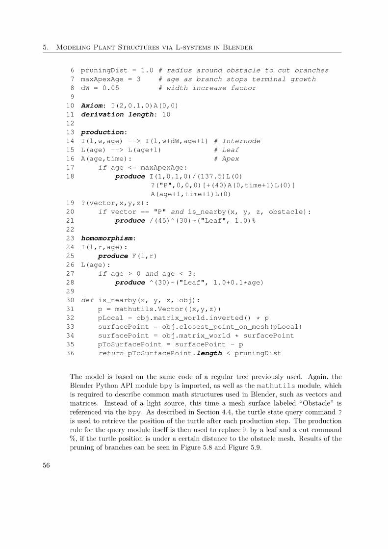
5. Modeling Plant Structures via L-systems in Blender

6 pruningDist = 1.0 # radius around obstacle to cut branches7 maxApexAge = 3 # age as branch stops terminal growth8 dW = 0.05 # width increase factor910 Axiom: I(2,0.1,0)A(0,0)11 derivation length: 101213 production:14 I(l,w,age) --> I(l,w+dW,age+1) # Internode15 L(age) --> L(age+1) # Leaf16 A(age,time): # Apex17 if age <= maxApexAge:18 produce I(1,0.1,0)/(137.5)L(0)

?("P",0,0,0)[+(40)A(0,time+1)L(0)]A(age+1,time+1)L(0)

19 ?(vector,x,y,z):20 if vector == "P" and is_nearby(x, y, z, obstacle):21 produce /(45)^(30)~("Leaf", 1.0)%2223 homomorphism:24 I(l,r,age):25 produce F(l,r)26 L(age):27 if age > 0 and age < 3:28 produce ^(30)~("Leaf", 1.0+0.1*age)2930 def is_nearby(x, y, z, obj):31 p = mathutils.Vector((x,y,z))32 pLocal = obj.matrix_world.inverted() * p33 surfacePoint = obj.closest_point_on_mesh(pLocal)34 surfacePoint = obj.matrix_world * surfacePoint35 pToSurfacePoint = surfacePoint - p36 return pToSurfacePoint.length < pruningDist

The model is based on the same code of a regular tree previously used. Again, theBlender Python API module bpy is imported, as well as the mathutils module, whichis required to describe common math structures used in Blender, such as vectors andmatrices. Instead of a light source, this time a mesh surface labeled “Obstacle” isreferenced via the bpy. As described in Section 4.4, the turtle state query command ?is used to retrieve the position of the turtle after each production step. The productionrule for the query module itself is then used to replace it by a leaf and a cut command%, if the turtle position is under a certain distance to the obstacle mesh. Results of thepruning of branches can be seen in Figure 5.8 and Figure 5.9.

56

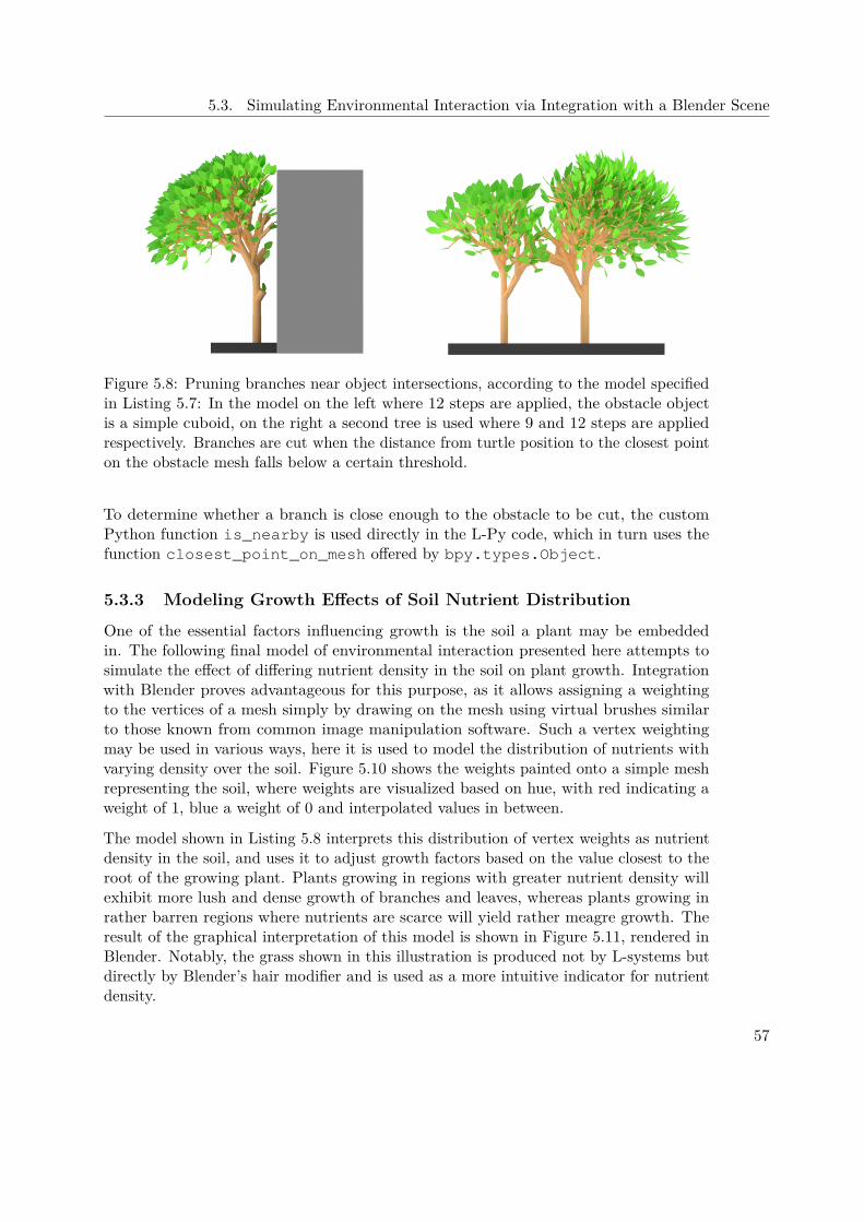
5.3. Simulating Environmental Interaction via Integration with a Blender Scene

Figure 5.8: Pruning branches near object intersections, according to the model specifiedin Listing 5.7: In the model on the left where 12 steps are applied, the obstacle objectis a simple cuboid, on the right a second tree is used where 9 and 12 steps are appliedrespectively. Branches are cut when the distance from turtle position to the closest pointon the obstacle mesh falls below a certain threshold.

To determine whether a branch is close enough to the obstacle to be cut, the customPython function is_nearby is used directly in the L-Py code, which in turn uses thefunction closest_point_on_mesh offered by bpy.types.Object.

5.3.3 Modeling Growth Effects of Soil Nutrient Distribution

One of the essential factors influencing growth is the soil a plant may be embeddedin. The following final model of environmental interaction presented here attempts tosimulate the effect of differing nutrient density in the soil on plant growth. Integrationwith Blender proves advantageous for this purpose, as it allows assigning a weightingto the vertices of a mesh simply by drawing on the mesh using virtual brushes similarto those known from common image manipulation software. Such a vertex weightingmay be used in various ways, here it is used to model the distribution of nutrients withvarying density over the soil. Figure 5.10 shows the weights painted onto a simple meshrepresenting the soil, where weights are visualized based on hue, with red indicating aweight of 1, blue a weight of 0 and interpolated values in between.

The model shown in Listing 5.8 interprets this distribution of vertex weights as nutrientdensity in the soil, and uses it to adjust growth factors based on the value closest to theroot of the growing plant. Plants growing in regions with greater nutrient density willexhibit more lush and dense growth of branches and leaves, whereas plants growing inrather barren regions where nutrients are scarce will yield rather meagre growth. Theresult of the graphical interpretation of this model is shown in Figure 5.11, rendered inBlender. Notably, the grass shown in this illustration is produced not by L-systems butdirectly by Blender’s hair modifier and is used as a more intuitive indicator for nutrientdensity.

57

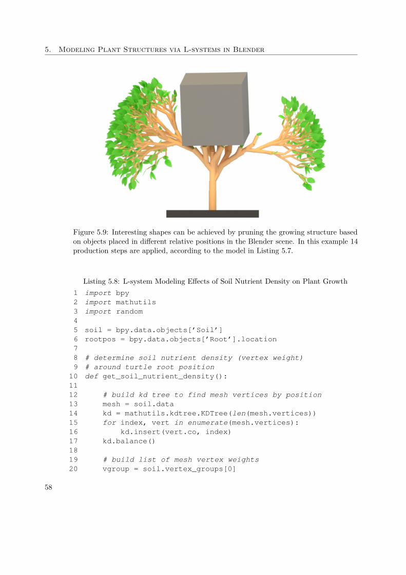
5. Modeling Plant Structures via L-systems in Blender

Figure 5.9: Interesting shapes can be achieved by pruning the growing structure basedon objects placed in different relative positions in the Blender scene. In this example 14production steps are applied, according to the model in Listing 5.7.

Listing 5.8: L-system Modeling Effects of Soil Nutrient Density on Plant Growth1 import bpy2 import mathutils3 import random45 soil = bpy.data.objects[’Soil’]6 rootpos = bpy.data.objects[’Root’].location78 # determine soil nutrient density (vertex weight)9 # around turtle root position10 def get_soil_nutrient_density():1112 # build kd tree to find mesh vertices by position13 mesh = soil.data14 kd = mathutils.kdtree.KDTree(len(mesh.vertices))15 for index, vert in enumerate(mesh.vertices):16 kd.insert(vert.co, index)17 kd.balance()1819 # build list of mesh vertex weights20 vgroup = soil.vertex_groups[0]

58

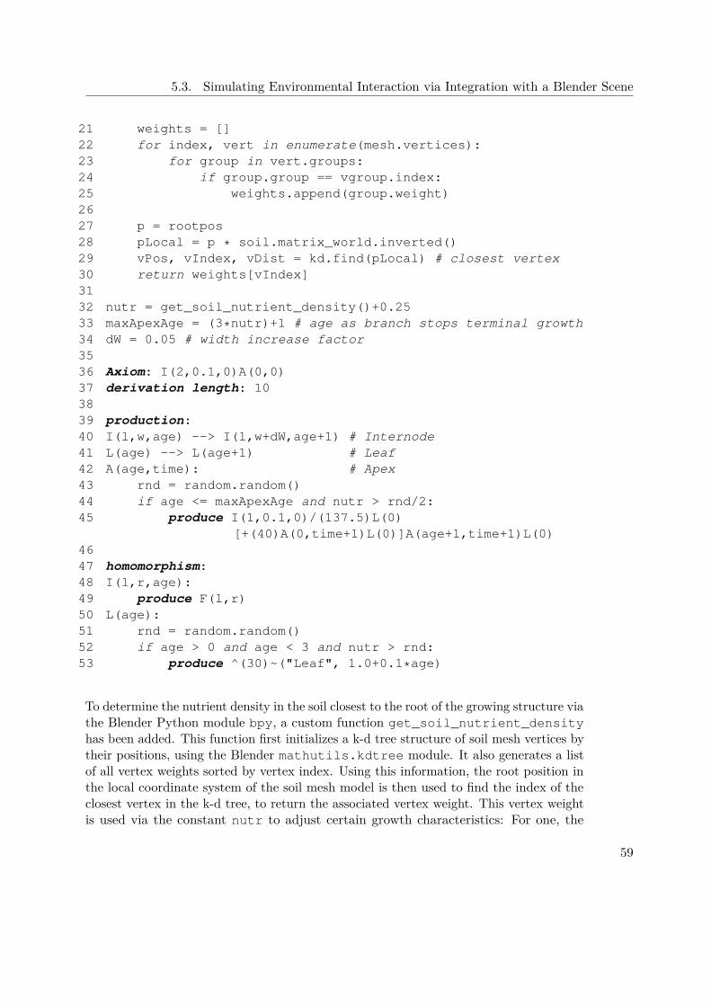
5.3. Simulating Environmental Interaction via Integration with a Blender Scene

21 weights = []22 for index, vert in enumerate(mesh.vertices):23 for group in vert.groups:24 if group.group == vgroup.index:25 weights.append(group.weight)2627 p = rootpos28 pLocal = p * soil.matrix_world.inverted()29 vPos, vIndex, vDist = kd.find(pLocal) # closest vertex30 return weights[vIndex]3132 nutr = get_soil_nutrient_density()+0.2533 maxApexAge = (3*nutr)+1 # age as branch stops terminal growth34 dW = 0.05 # width increase factor3536 Axiom: I(2,0.1,0)A(0,0)37 derivation length: 103839 production:40 I(l,w,age) --> I(l,w+dW,age+1) # Internode41 L(age) --> L(age+1) # Leaf42 A(age,time): # Apex43 rnd = random.random()44 if age <= maxApexAge and nutr > rnd/2:45 produce I(1,0.1,0)/(137.5)L(0)

[+(40)A(0,time+1)L(0)]A(age+1,time+1)L(0)4647 homomorphism:48 I(l,r,age):49 produce F(l,r)50 L(age):51 rnd = random.random()52 if age > 0 and age < 3 and nutr > rnd:53 produce ^(30)~("Leaf", 1.0+0.1*age)

To determine the nutrient density in the soil closest to the root of the growing structure viathe Blender Python module bpy, a custom function get_soil_nutrient_densityhas been added. This function first initializes a k-d tree structure of soil mesh vertices bytheir positions, using the Blender mathutils.kdtree module. It also generates a listof all vertex weights sorted by vertex index. Using this information, the root position inthe local coordinate system of the soil mesh model is then used to find the index of theclosest vertex in the k-d tree, to return the associated vertex weight. This vertex weightis used via the constant nutr to adjust certain growth characteristics: For one, the

59

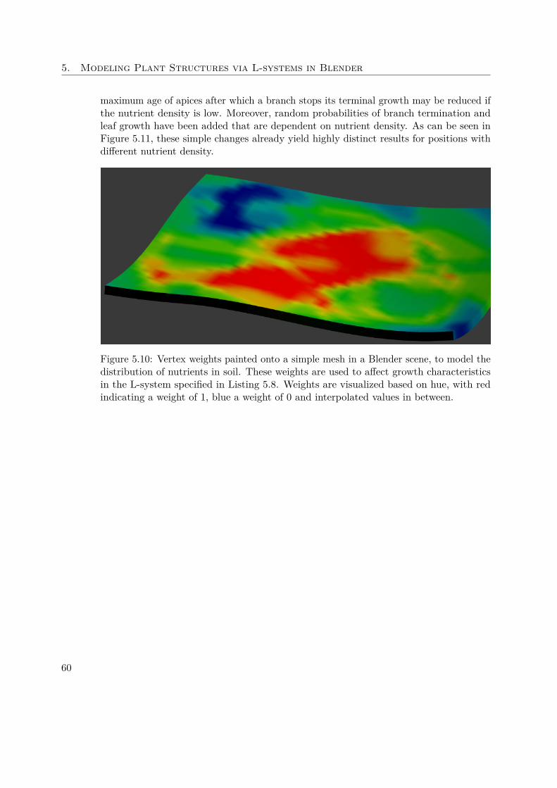
5. Modeling Plant Structures via L-systems in Blender

maximum age of apices after which a branch stops its terminal growth may be reduced ifthe nutrient density is low. Moreover, random probabilities of branch termination andleaf growth have been added that are dependent on nutrient density. As can be seen inFigure 5.11, these simple changes already yield highly distinct results for positions withdifferent nutrient density.

Figure 5.10: Vertex weights painted onto a simple mesh in a Blender scene, to model thedistribution of nutrients in soil. These weights are used to affect growth characteristicsin the L-system specified in Listing 5.8. Weights are visualized based on hue, with redindicating a weight of 1, blue a weight of 0 and interpolated values in between.

60

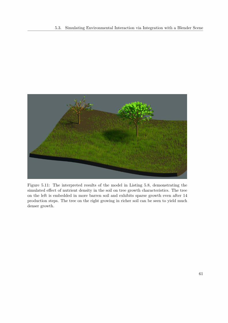
5.3. Simulating Environmental Interaction via Integration with a Blender Scene

Figure 5.11: The interpreted results of the model in Listing 5.8, demonstrating thesimulated effect of nutrient density in the soil on tree growth characteristics. The treeon the left is embedded in more barren soil and exhibits sparse growth even after 14production steps. The tree on the right growing in richer soil can be seen to yield muchdenser growth.

61

CHAPTER 6Conclusion and Possible

Improvements

Today, Lindenmayer systems are used for a wide range of applications in the fieldof procedural modeling. It may be argued that the focus has shifted more towardarchitectural man-made structures, as far as the modeling of whole urban city structuresbased on L-systems as presented by Parish and Müller [PM01]. However, as emphasized byWonka and Wimmer [WWSR03] in their approach to modeling buildings, the generationof architectural models is generally characterized by a partitioning process rather than agrowth process, thus proving other shape grammars more suitable.

The use of L-systems for the modeling of plants likewise is more of a niche interest today.This is mainly due to them being rendered obsolete by the existence of other modelingapproaches: Methods better suited for artistic aesthetic use that yield more predictableand intuitive results to work with as an artist, as discussed in Chapter 2, as well as moredetailed biological models hard to capture via L-systems. Nonetheless, L-systems in thefield of plant modeling still produce a plethora of fascinating forms and patterns, thestudy of which is highly interesting and worthwhile in itself. Likely the most potentialapplication today would thus be in the educational field, as discussed among others byHanan [Han92] and Boudon et al. [BPC+12].

The focus of this work was, however, not to present novel techniques for the aesthetic orbiological modeling of plants. The main goal of this work was to integrate the existingformalism of parametric context-sensitive L-systems in the open-source computer graphicssoftware Blender, with special consideration on allowing the modeling of environmentalinteraction with a Blender scene, and more importantly to discuss the possible resultsand potential of such an integration.

63

6. Conclusion and Possible Improvements

In Chapter 3 the well-established theory of L-systems was laid out as an overview, followedby a brief review of the various extensions that have been introduced to the L-systemformalism over the years.

Building on this foundation, Chapter 4 discussed the implementation steps required tobring L-systems to Blender. This was done in the form of a small add-on that uses anadapted version of the open-source L-Py L-system framework for L-string production, aswell as independent graphical interpretation code based specifically on the Blender PythonAPI with extended interpretation commands to facilitate environmental interaction witha Blender scene. Chapter 4 also discussed potential advantages of this integration inBlender from a theoretical standpoint, which were then verified via application results inChapter 5.

Finally, Chapter 5 demonstrated results of L-Py integration in Blender for environmentalinteraction with Blender scene context during L-system production, post-productionmodeling and simulation tools as well as rendering. This was done via examples ofmodeled results for plant inflorescence and tree structures, the main focus howeverbeing the discussion of environmental interaction which is arguably the most promisingapplication of Blender integration.

To conclude, it can be said that integration of L-system production and interpretationwith a highly versatile computer graphics software like Blender may greatly enhancethe overall visibility and interest of L-systems with regards to a large audience of users.Direct integration with a commonly used modeling and rendering tool makes it easierto visualize produced models and customize them after L-system production, as well aspresenting them in the context of a complex environment such as a Blender scene. Mostimportantly, however, there is great potential to influence the actual production of thegrowing structure based on such context to model environmental interaction.

Several improvements to the add-on implementation may be desirable, some of themmentioned in the following:

• Rebuild L-Py in pure Python to achieve platform independence and greater ease ofuse. The performance penalty compared to the current C++ wrapper might beconsiderable though.

• Allow for the generation of smoothly curved internodes.

• Generate Blender mesh structures from individual vertices directly in L-Py, asopposed to using existing mesh objects. This may be possible via the featuresoffered by the Blender Python API. While it may not be very intuitive to modelmesh structures from code, it would be useful for the modeling of proceduralvariation in the structures of leaves and other plant organs.

• Implement modular L-systems where a module in one L-system may trigger produc-tion rules of another L-system, i.e., to allow for two mutually influencing growingstructures without having to manually produce and then reference resulting objects.

64

• Add more sophisticated tools to model environmental interaction and influence ofthe environmental context on the growing structure with more precise control.

65

Bibliography

[AK84] Masaki Aono and Tosiyasu Kunii. Botanical tree image generation. IEEEComput. Graph. Appl., 4(5):10–34, May 1984.

[BPC+12] Frédéric Boudon, Christophe Pradal, Thomas Cokelaer, PrzemyslawPrusinkiewicz, and Christophe Godin. L-Py: An L-system SimulationFramework for Modeling Plant Architecture Development Based on aDynamic Language. Frontiers in Plant Science, 3(76):doi: 10.3389/f-pls.2012.00076, May 2012.

[Bur13] Thomas Burt. Interactive Evolutionary Modelling by Duplication andDiversification of L-Systems. PhD thesis, University of Calgary, 2013.

[dREF+88] Phillippe de Reffye, Claude Edelin, Jean Françon, Marc Jaeger, and ClaudePuech. Plant Models Faithful to Botanical Structure and Development.SIGGRAPH Comput. Graph., 22(4):151–158, June 1988.

[dReIeeA14] INRIA Institut National de Recherche en Informatique et en Automatique.OpenAlea Software Environment for Plant Modeling. http://openalea.gforge.inria.fr, 2014. Acessed: 2017-01-31.

[dReIeeA16a] INRIA Institut National de Recherche en Informatique et enAutomatique. L-Py Open Source Lindenmayer Systems forPython. Developer Documentation. http://openalea.gforge.inria.fr/dokuwiki/doku.php?id=packages:vplants:lpy:doc#developper_documentation, 2016. Accessed: 2017-03-03.

[dReIeeA16b] INRIA Institut National de Recherche en Informatique et en Automatique.L-Py Open Source Lindenmayer Systems for Python. GitHub Repository.https://github.com/openalea/lpy, 2016. Accessed: 2017-03-03.

[dReIeeA16c] INRIA Institut National de Recherche en Informatique et en Au-tomatique. L-Py Open Source Lindenmayer Systems for Python.Main Page. http://openalea.gforge.inria.fr/dokuwiki/doku.php?id=packages:vplants:lpy:main, 2016. Accessed: 2017-02-04.

67

[ES80] Peter Eichhorst and Walter J Savitch. Growth functions of stochasticlindenmayer systems. Information and Control, 45(3):217–228, 1980.

[Fal90] Kenneth Falconer. Fractal Geometry: Mathematical Foundations andApplications. John Wiley & Sons, 1990.

[Fou09] The Python Software Foundation. What’s New In Python 3.0. https://docs.python.org/3.0/whatsnew/3.0.html, 2009. Accessed: 2017-03-03.

[FtBC09] Blender Foundation and the Blender Community. Blender Python 3.xMigration Proposal. https://wiki.blender.org/index.php/Dev:2.5/Source/Python/API/Py3.1_Migration, 2009. Accessed: 2017-03-03.

[FtBC16] Blender Foundation and the Blender Community. Blender 2.78 PythonAPI Documentation. https://docs.blender.org/api/blender_python_api_2_78_release, 2016. Accessed: 2017-01-31.

[FtBC17a] Blender Foundation and the Blender Community. Blender 2.78 Config-uring Platform Dependent Paths. https://blender.org/manual/getting_started/installing/configuration/directories.html, 2017. Accessed: 2017-03-03.

[FtBC17b] Blender Foundation and the Blender Community. Blender Reference Man-ual. https://docs.blender.org/manual/en/dev, 2017. Accessed:2017-03-04.

[FtBC17c] Blender Foundation and the Blender Community. blender.org: Homeof the Blender project. Free and Open 3D Creation Software. https://blender.org, 2017. Accessed: 2017-01-31.

[Ham96] Mark Stephen Hammel. Differential L-systems and their application tothe simulation and visualisation of plant development. Computer Science,University of Calgary, 1996.

[Han92] James Scott Hanan. Parametric L-systems and Their Application to theModelling and Visualization of Plants. PhD thesis, 1992.

[Hon71] Hisao Honda. Description of the form of trees by the parameters of thetree-like body: Effects of the branching angle and the branch length on theshape of the tree-like body. Journal of theoretical biology, 31(2):331–338,1971.

[JL87] J. M. Janssen and A. Lindenmayer. Models for the control of branchpositions and flowering sequences of capitula in mycelis muralis (l.) dumont(compositae). New Phytologist, 105(2):191–220, 1987.

68

[KK08] Ole Kniemeyer and Winfried Kurth. The Modelling Platform GroIMP andthe Programming Language XL, pages 570–572. Springer Berlin Heidelberg,Berlin, Heidelberg, 2008.

[KP03] Radoslaw Karwowski and Przemyslaw Prusinkiewicz. Design and Imple-mentation of the L+C Modeling Panguage. Electronic Notes in TheoreticalComputer Science, 86(2):134–152, 2003.

[LD98] Bernd Lintermann and Oliver Deussen. A Modelling Method and UserInterface for Creating Plants. Computer Graphics Forum, 1998.

[LD99] Bernd Lintermann and Oliver Deussen. Interactive Modeling of Plants.IEEE Comput. Graph. Appl., 19(1):56–65, January 1999.

[Leo17] Niko Leopold. Lindenmaker: A Blender add-on for Lindenmayer systems(L-systems) using the L-Py Python library. https://github.com/mangostaniko/lpy-lsystems-blender-addon, 2017. Accessed:2017-08-31.

[Lin68] Aristid Lindenmayer. Mathematical Models for Cellular Interactions inDevelopment II. Simple and Branching Filaments with Two-sided Inputs.Journal of theoretical biology, 18(3):280–299, 1968.

[LR79] Aristid Lindenmayer and Grzegorz Rozenberg. Parallel generation ofmaps: Developmental systems for cell layers. In Graph-grammars andtheir application to computer science and biology, pages 301–316. Springer,1979.

[Mac93] Cameron MacKenzie. Artificial Evolution of Generative Models in Com-puter Graphics. Computer Science, University of Calgary, 1993.

[Man83] B. B. Mandelbrot. The Fractal Geometry of Nature. W. H. Freeman andComp., New York, 3 edition, 1983.

[MP96] Radomír Měch and Przemyslaw Prusinkiewicz. Visual models of plantsinteracting with their environment. In Proceedings of the 23rd annualconference on Computer graphics and interactive techniques, pages 397–410.ACM, 1996.

[MPH90] Lynn Mercer, Przemyslaw Prusinkiewicz, and James Hanan. The conceptand design of a virtual laboratory. Proceedings of Graphics Interface.Halifax, Nova Scotia, 90:149–155, 1990.

[PHHM97a] P. Prusinkiewicz, M. Hammel, J. Hanan, and R. Mech. L-systems: Fromthe Theory to Visual Models of Plants. In M. T. Michalewicz, editor,Plants to Ecosystems. Advances in Computational Life Sciences, I. CSIROpublishing, Melbourne, 1997.

69

[PHHM97b] Przemyslaw Prusinkiewicz, Mark Hammel, Jim Hanan, and Radomír Měch.Visual Models of Plant Development. In Handbook of formal languages,pages 535–597. Springer, 1997.

[PHM99] Przemyslaw Prusinkiewicz, Jim Hanan, and Radomír Měch. An L-system-based Plant Modeling Language. In Applications of graph transformationswith industrial relevance, pages 395–410. Springer, 1999.

[PHMH95] Przemyslaw Prusinkiewicz, Mark Hammel, Radomir Mech, and Jim Hanan.The Artificial Life of Plants. Artificial life for graphics, animation, andvirtual reality, 7, 1995.

[PKL07] Przemyslaw Prusinkiewicz, Radoslaw Karwowski, and Brendan Lane. TheL+C Plant-Modelling Language. Frontis, 22:27–42, 2007.

[PL96] Przemyslaw Prusinkiewicz and Aristid Lindenmayer. The AlgorithmicBeauty of Plants. Springer-Verlag New York, Inc., New York, NY, USA,1996.

[PM01] Yoav IH Parish and Pascal Müller. Procedural modeling of cities. InProceedings of the 28th annual conference on Computer graphics andinteractive techniques, pages 301–308. ACM, 2001.

[Pru93] Przemyslaw Prusinkiewicz. Modelling and Visualization of Biological Struc-tures. In Proceedings of Graphics Interface ’93, GI ’93, pages 128–137,Toronto, Ontario, Canada, 1993. Canadian Human-Computer Communi-cations Socitey.

[Pru98] Przemyslaw Prusinkiewicz. Modeling of Spatial Structure and Developmentof Plants: A Review. Scientia Horticulturae, 74(1):113–149, 1998.

[Pru99] Przemyslaw Prusinkiewicz. A Look at the Visual Modeling of Plants UsingL-systems. Agronomie, 19(3/4):211–224, 1999.

[Pru00] Przemyslaw Prusinkiewicz. Simulation Modeling of Plants and PlantEcosystems. Communications of the ACM, 43(7):84–93, July 2000.

[Pru04] Przemyslaw Prusinkiewicz. Art and Science of Life: Designing and Grow-ing Virtual Plants with L-systems. In XXVI International HorticulturalCongress: Nursery Crops; Development, Evaluation, Production and Use630, pages 15–28, 2004.

[RB85] William T Reeves and Ricki Blau. Approximate and probabilistic algo-rithms for shading and rendering structured particle systems. In ACMSiggraph Computer Graphics, volume 19, pages 313–322. ACM, 1985.

70

[RCSL03] Yodthong Rodkaew, Prabhas Chongstitvatana, Suchada Siripant, andChidchanok Lursinsap. Particle Systems for Plant Modeling. Plant growthmodeling and applications, pages 210–217, 2003.

[RLP07] Adam Runions, Brendan Lane, and Przemyslaw Prusinkiewicz. ModelingTrees with a Space Colonization Algorithm. In D. Ebert and S. Merillou,editors, Eurographics Workshop on Natural Phenomena. The EurographicsAssociation, 2007.

[Rob86] D. F. Robinson. A notation for the growth of inflorescences. New phytologist,103(3):587–596, 1986.

[Smi84] Alvy Ray Smith. Plants, Fractals, and Formal Languages. SIGGRAPHComput. Graph., 18(3), January 1984.

[Tur52] Alan Mathison Turing. The chemical basis of morphogenesis. Philosoph-ical Transactions of the Royal Society of London B: Biological Sciences,237(641):37–72, 1952.

[WP95] Jason Weber and Joseph Penn. Creation and Rendering of Realistic Trees.In Proceedings of the 22Nd Annual Conference on Computer Graphics andInteractive Techniques, SIGGRAPH ’95, pages 119–128, New York, NY,USA, 1995. ACM.

[WWSR03] Peter Wonka, Michael Wimmer, Franc cois Sillion, and William Ribarsky.Instant architecture. ACM Transaction on Graphics, 22(3):669–677, July2003. Proceedings ACM SIGGRAPH 2003.

71