Algorithms & Applications in Computer Vision

Lihi Zelnik-Manor

Lecture 11: Structure from Motion

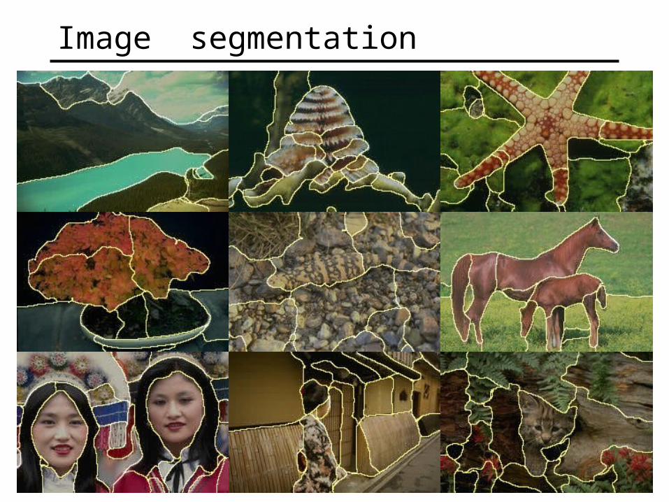
Image segmentation

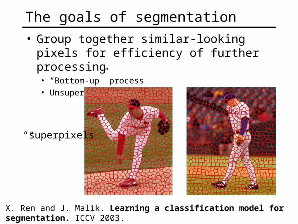
The goals of segmentation

• Group together similar-looking pixels for efficiency of further processing• “Bottom-up” process• Unsupervised

X. Ren and J. Malik. Learning a classification model for segmentation. ICCV 2003.

“superpixels”

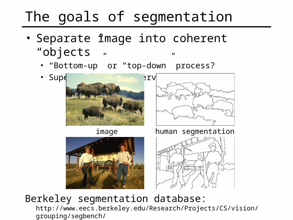
The goals of segmentation

• Separate image into coherent “objects”• “Bottom-up” or “top-down” process?• Supervised or unsupervised?

Berkeley segmentation database:http://www.eecs.berkeley.edu/Research/Projects/CS/vision/grouping/segbench/

image human segmentation

5

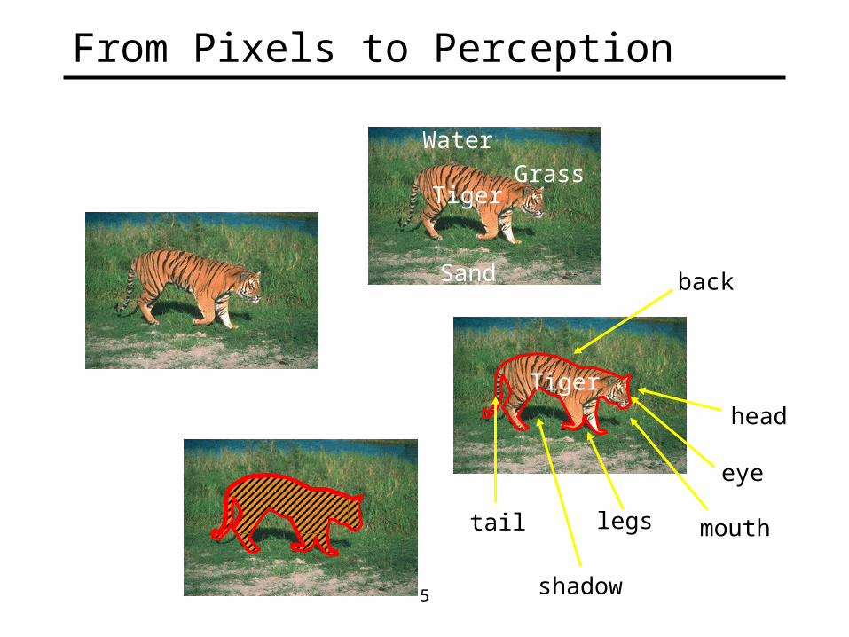
From Pixels to Perception

TigerGrass

Water

Sand

outdoorwildlife

Tiger

tail

eye

legs

head

back

shadow

mouth

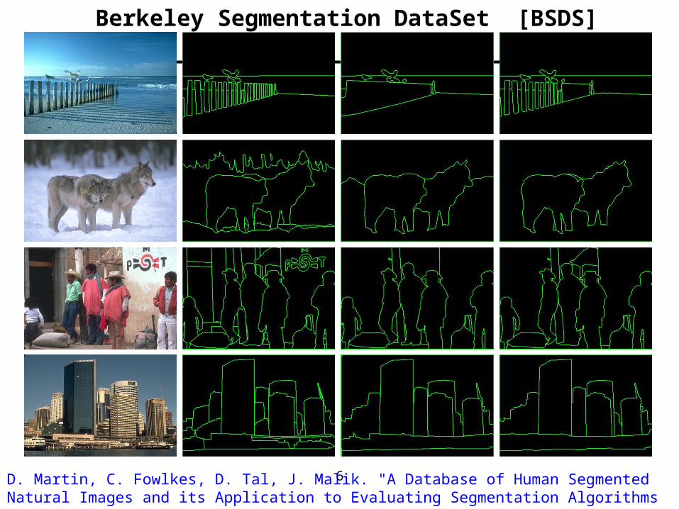
6D. Martin, C. Fowlkes, D. Tal, J. Malik. "A Database of Human Segmented Natural Images and its Application to Evaluating Segmentation Algorithms and Measuring Ecological Statistics", ICCV, 2001

Berkeley Segmentation DataSet [BSDS]

7

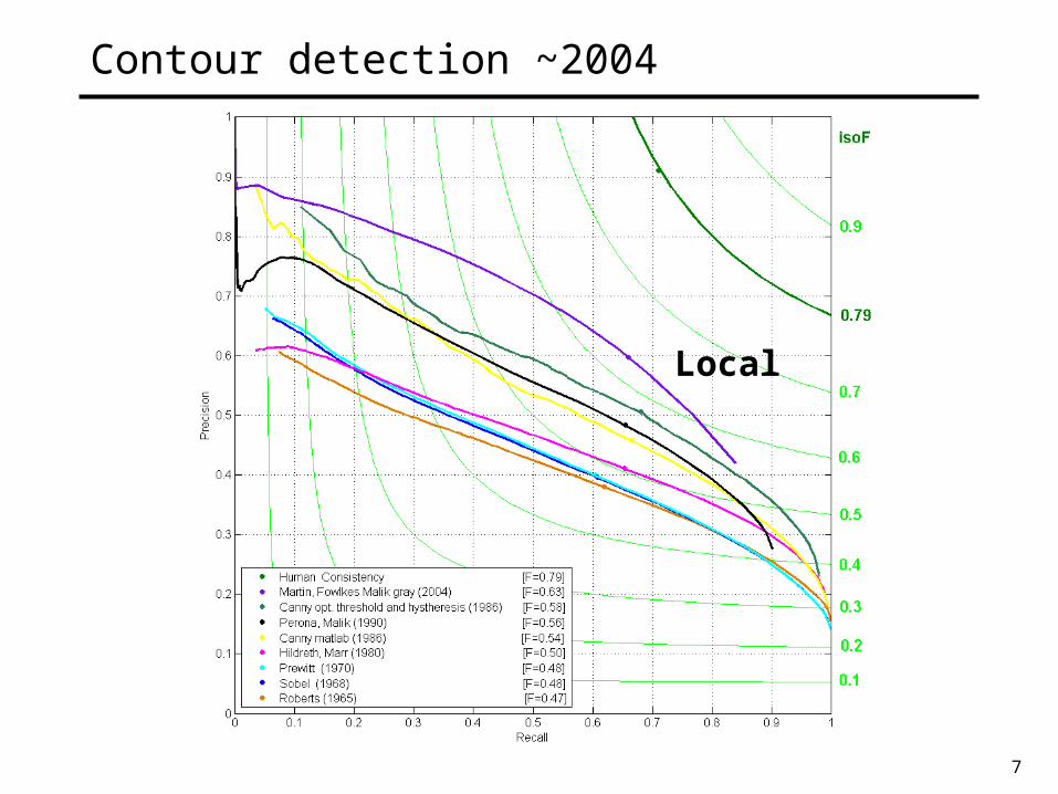
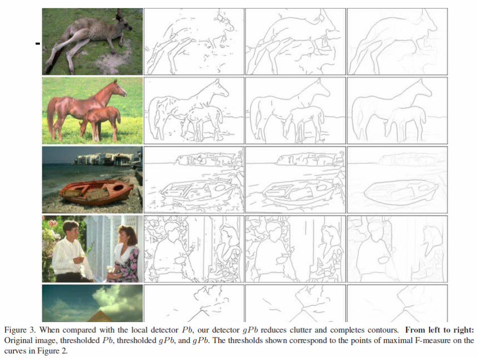
Contour detection ~2004

7

Local

8

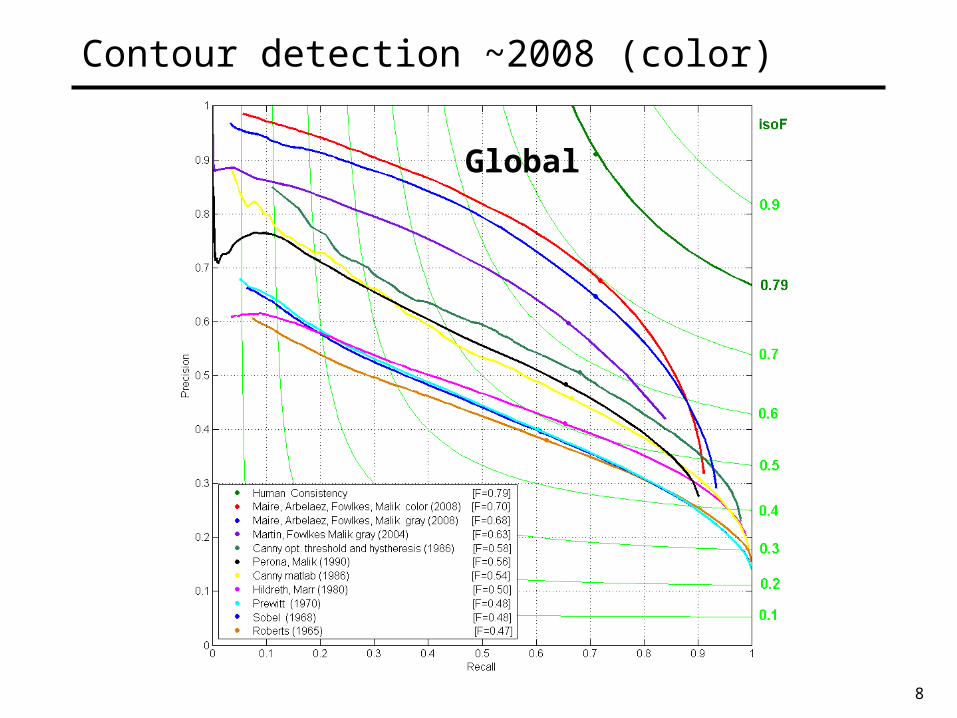
Contour detection ~2008 (color)

8

Global

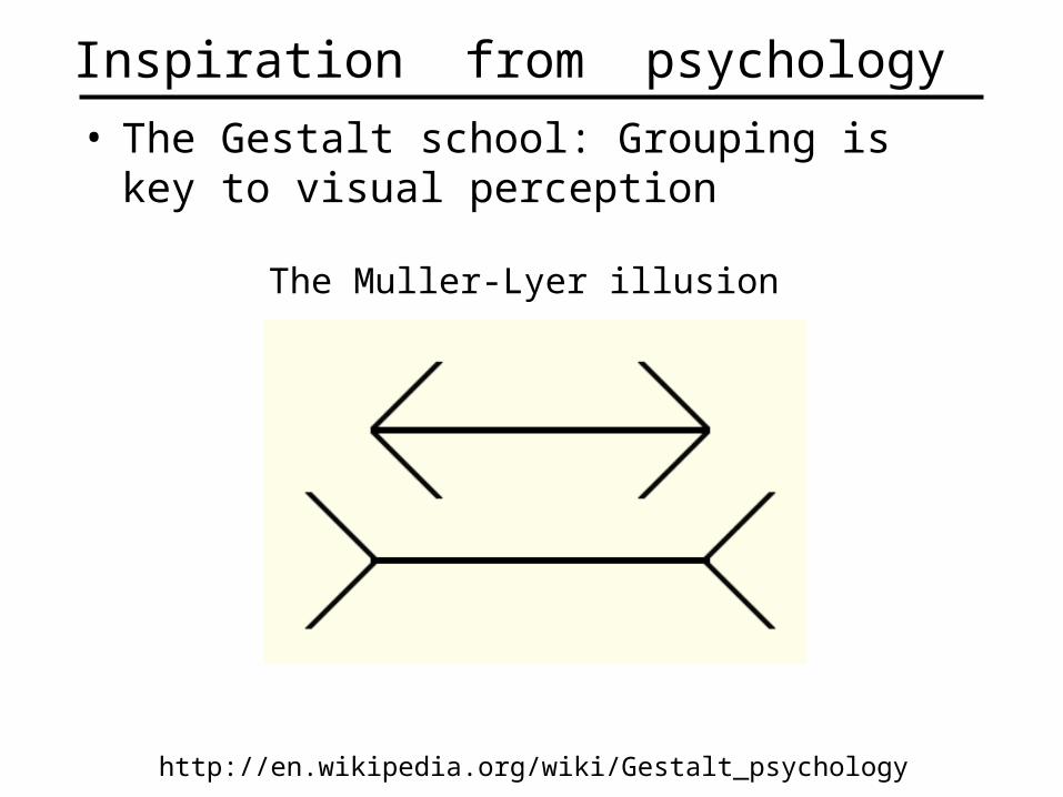
Inspiration from psychology

• The Gestalt school: Grouping is key to visual perception

The Muller-Lyer illusion

http://en.wikipedia.org/wiki/Gestalt_psychology

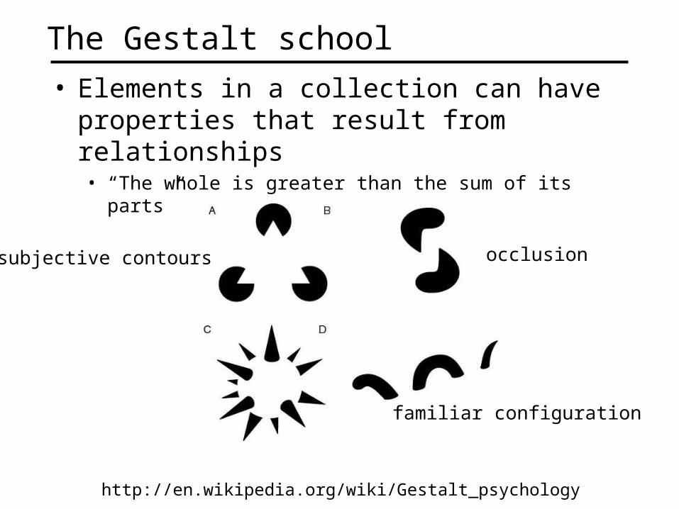
The Gestalt school

• Elements in a collection can have properties that result from relationships • “The whole is greater than the sum of its parts”

subjective contours occlusion

familiar configuration

http://en.wikipedia.org/wiki/Gestalt_psychology

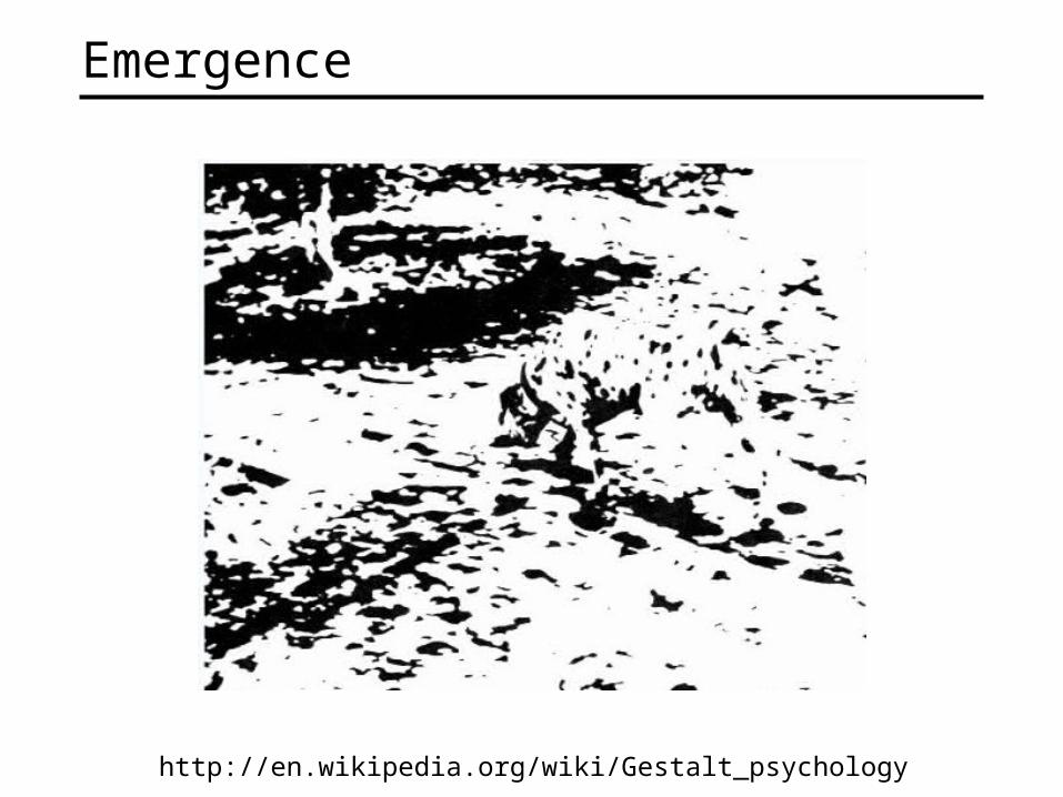
Emergence

http://en.wikipedia.org/wiki/Gestalt_psychology

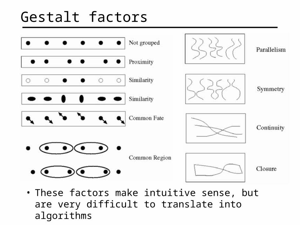
Gestalt factors

• These factors make intuitive sense, but are very difficult to translate into algorithms

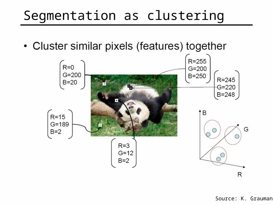
Segmentation as clustering

Source: K. Grauman

Two components to clustering

1. Similarity between pixels1. For now lets assume it is the distance between RGB

values.

2. The clustering algorithm

What is Clustering?What is Clustering?• Organizing data into classes such that:

• high intra-class similarity

• low inter-class similarity

• Finding the class labels and the number of classes directly from the data (in contrast to classification).

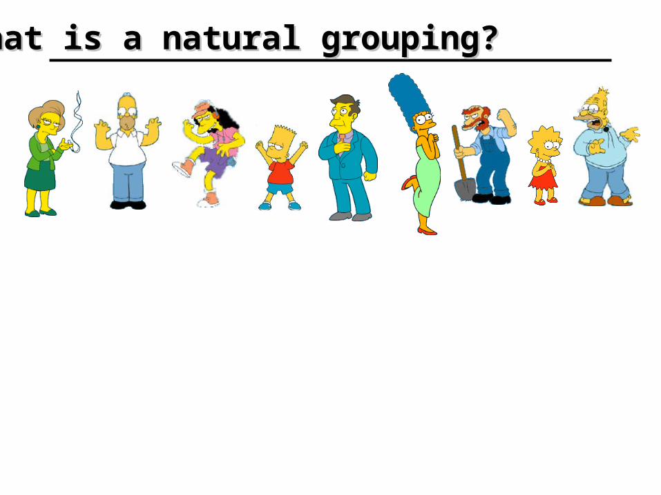
What is a natural grouping?What is a natural grouping?

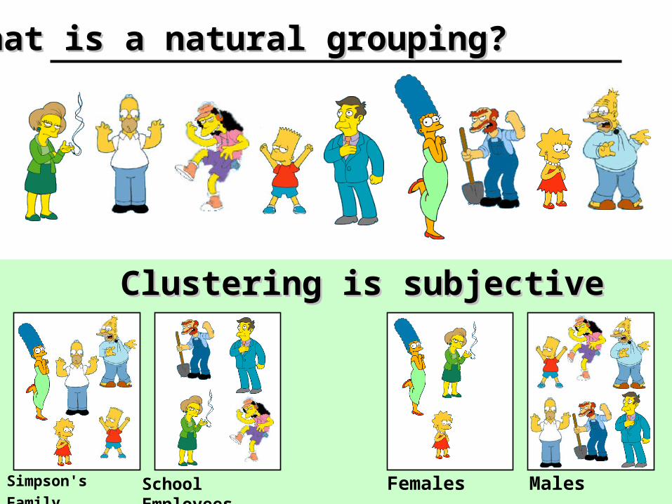
School Employees Simpson's Family Males Females

Clustering is subjectiveClustering is subjective

What is a natural grouping?What is a natural grouping?

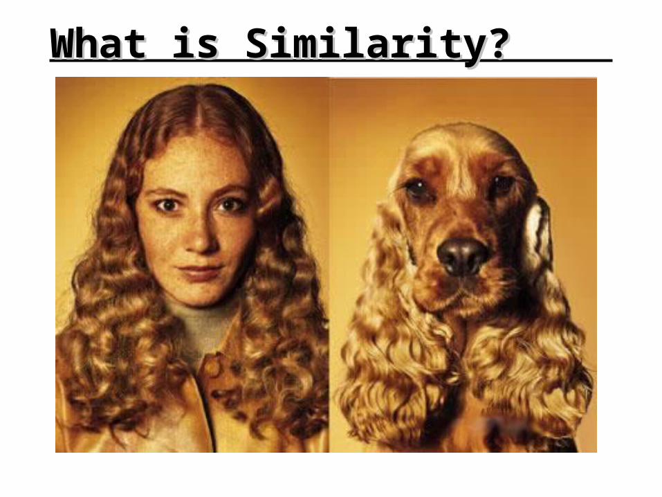
What is Similarity?What is Similarity?

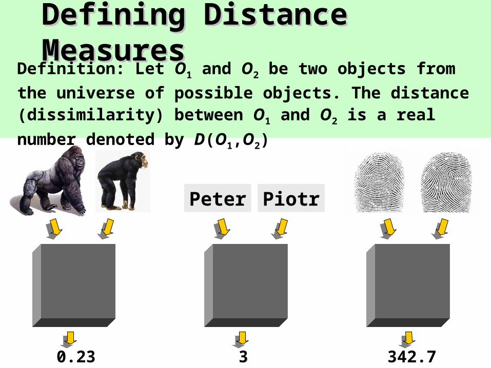
Defining Distance MeasuresDefining Distance MeasuresDefinition: Let O1 and O2 be two objects from the universe

of possible objects. The distance (dissimilarity) between O1 and O2 is a real number denoted by D(O1,O2)

0.23 3 342.7

Peter Piotr

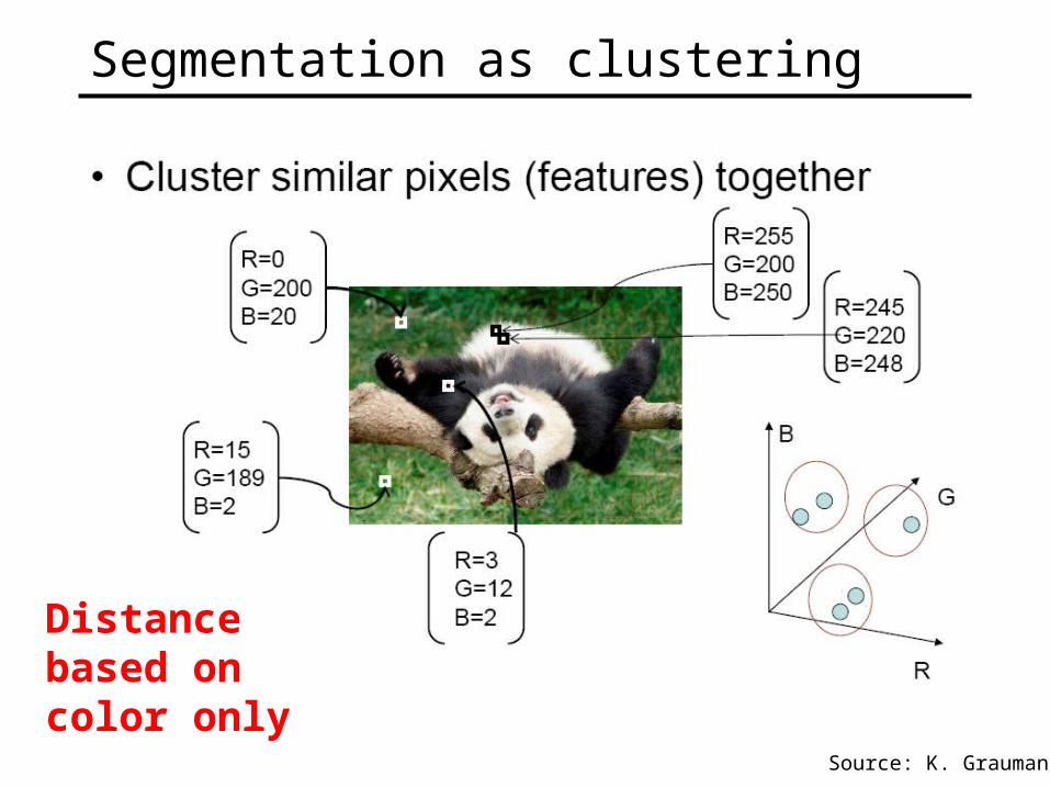
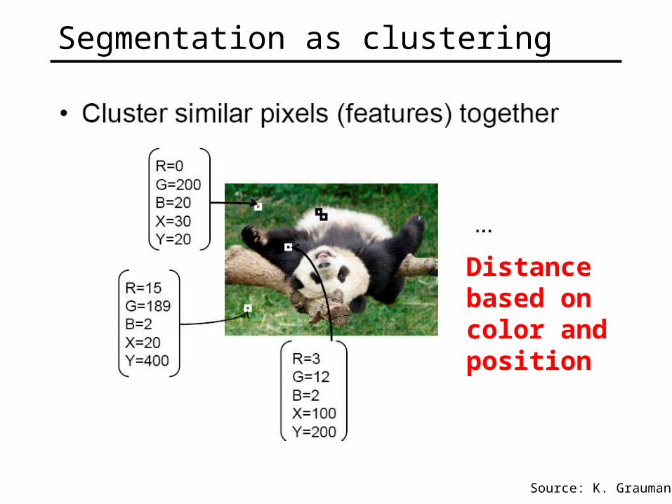
Segmentation as clustering

Source: K. Grauman

Distance based on color only

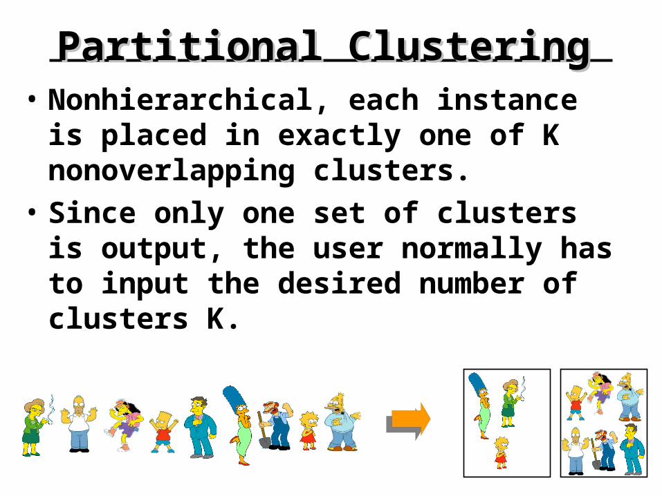
Partitional ClusteringPartitional Clustering• Nonhierarchical, each instance is placed

in exactly one of K nonoverlapping clusters.

• Since only one set of clusters is output, the user normally has to input the desired number of clusters K.

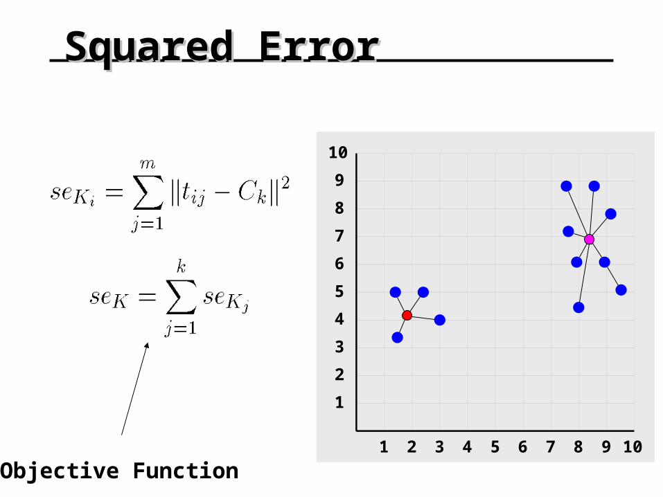
Squared ErrorSquared Error

10

1 2 3 4 5 6 7 8 9 10

1

2

3

4

5

6

7

8

9

Objective Function

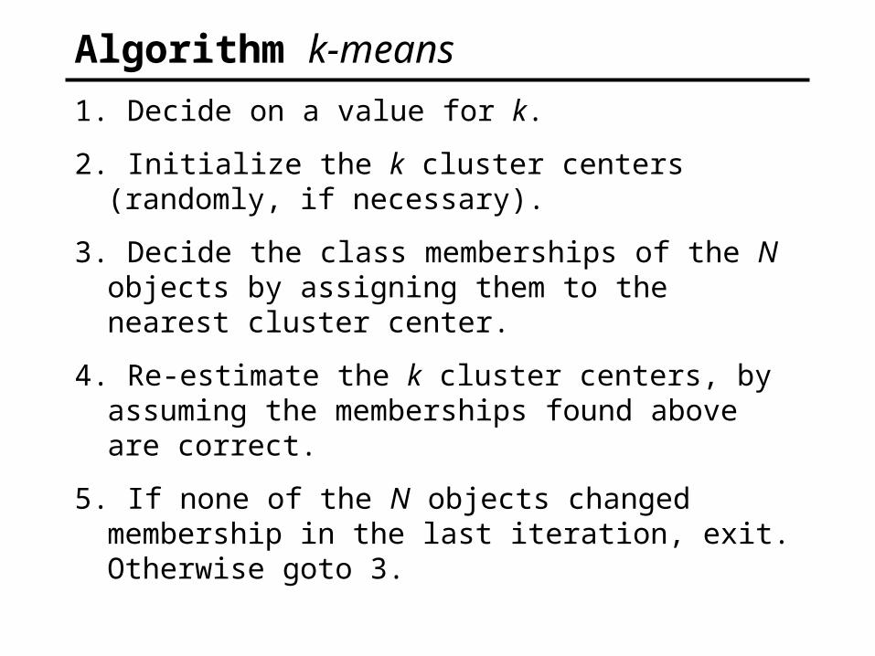
Algorithm k-means

1. Decide on a value for k.

2. Initialize the k cluster centers (randomly, if necessary).

3. Decide the class memberships of the N objects by assigning them to the nearest cluster center.

4. Re-estimate the k cluster centers, by assuming the memberships found above are correct.

5. If none of the N objects changed membership in the last iteration, exit. Otherwise goto 3.

0

1

2

3

4

5

0 1 2 3 4 5

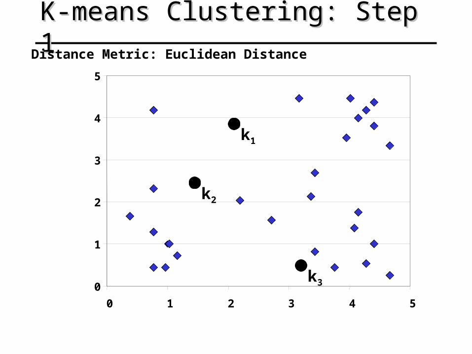
K-means Clustering: Step 1K-means Clustering: Step 1Distance Metric: Euclidean Distance

k1

k2

k3

0

1

2

3

4

5

0 1 2 3 4 5

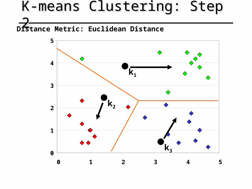
K-means Clustering: Step 2K-means Clustering: Step 2

k1

k2

k3

Distance Metric: Euclidean Distance

0

1

2

3

4

5

0 1 2 3 4 5

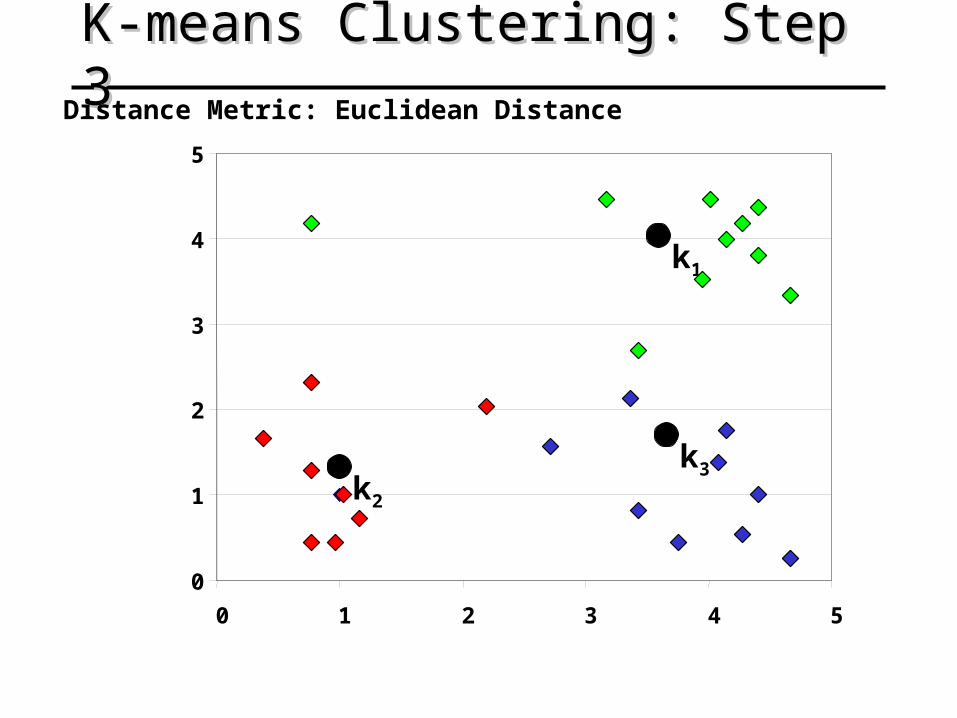
K-means Clustering: Step 3K-means Clustering: Step 3

k1

k2

k3

Distance Metric: Euclidean Distance

0

1

2

3

4

5

0 1 2 3 4 5

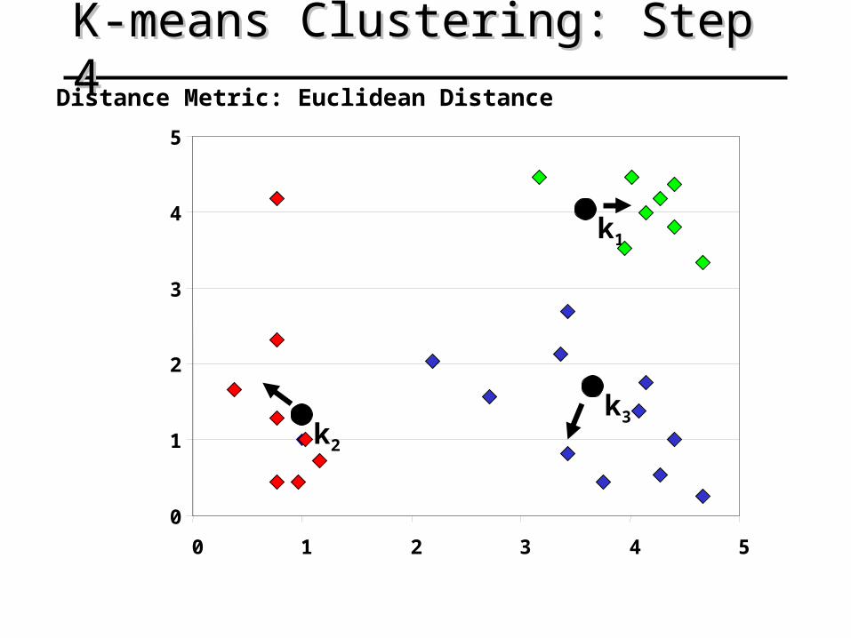
K-means Clustering: Step 4K-means Clustering: Step 4

k1

k2

k3

Distance Metric: Euclidean Distance

0

1

2

3

4

5

0 1 2 3 4 5

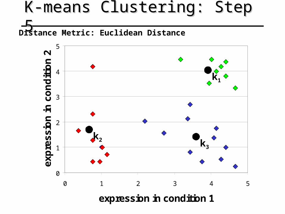
expression in condition 1

exp

ress

ion

in c

on

dit

ion

2

K-means Clustering: Step 5K-means Clustering: Step 5

k1

k2 k3

Distance Metric: Euclidean Distance

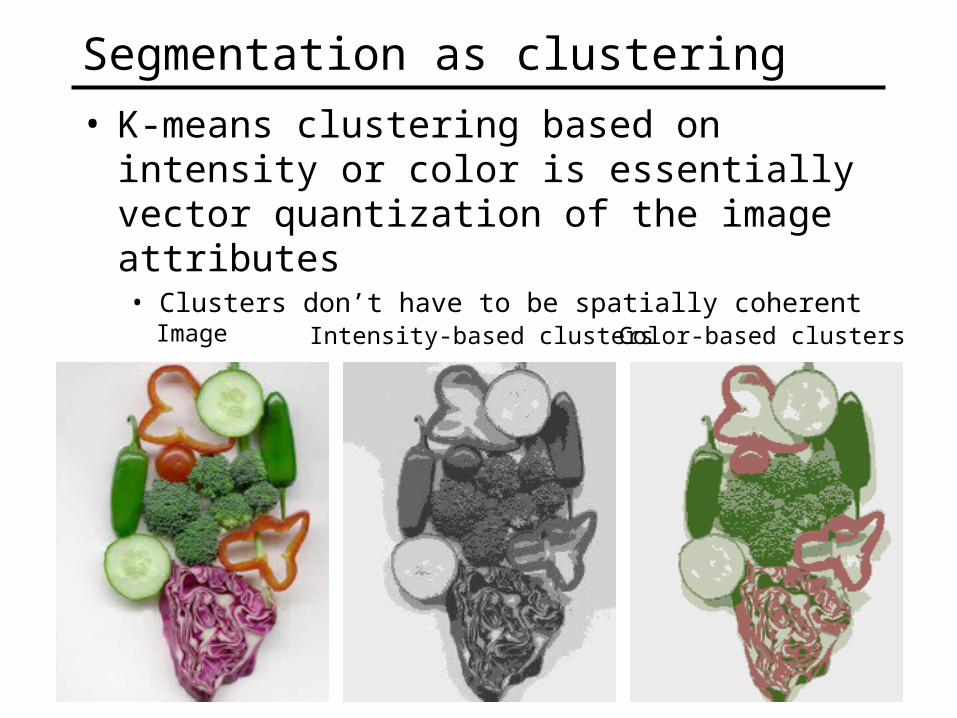
Image Intensity-based clusters Color-based clusters

Segmentation as clustering

• K-means clustering based on intensity or color is essentially vector quantization of the image attributes• Clusters don’t have to be spatially coherent

Segmentation as clustering

Source: K. Grauman

Distance based on color and position

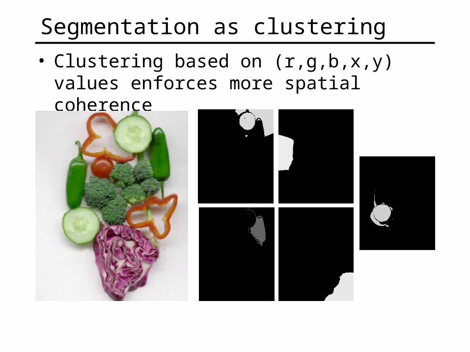
Segmentation as clustering

• Clustering based on (r,g,b,x,y) values enforces more spatial coherence

K-Means for segmentation

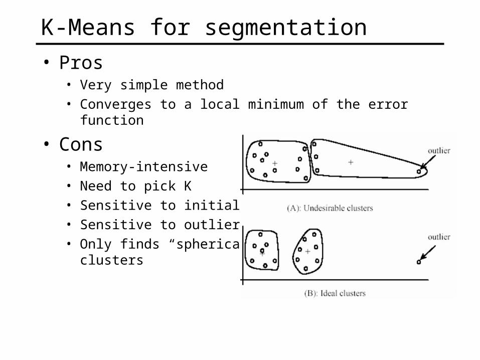
• Pros• Very simple method• Converges to a local minimum of the error function

• Cons• Memory-intensive• Need to pick K• Sensitive to initialization• Sensitive to outliers• Only finds “spherical”

clusters

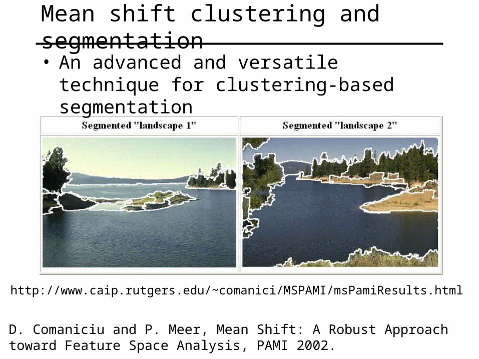
http://www.caip.rutgers.edu/~comanici/MSPAMI/msPamiResults.html

Mean shift clustering and segmentation

• An advanced and versatile technique for clustering-based segmentation

D. Comaniciu and P. Meer, Mean Shift: A Robust Approach toward Feature Space Analysis, PAMI 2002.

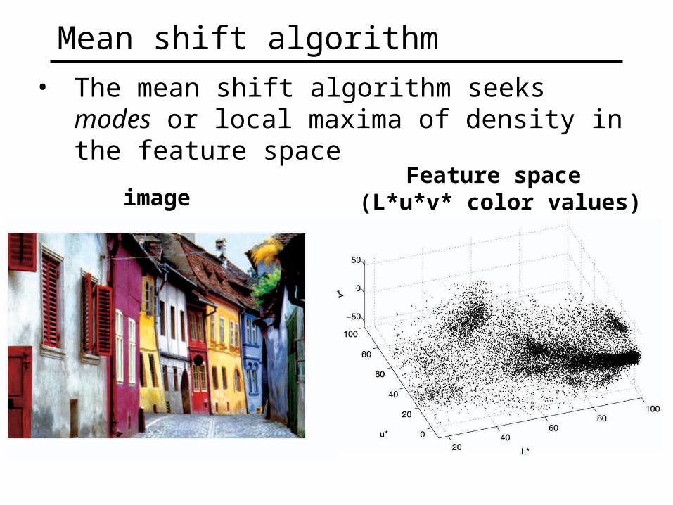
• The mean shift algorithm seeks modes or local maxima of density in the feature space

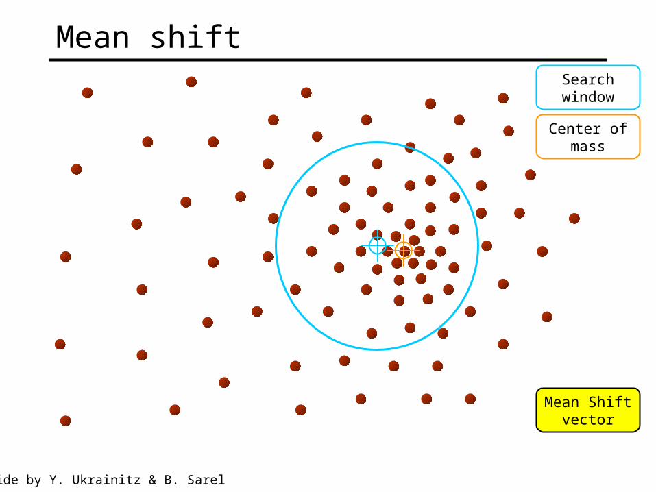
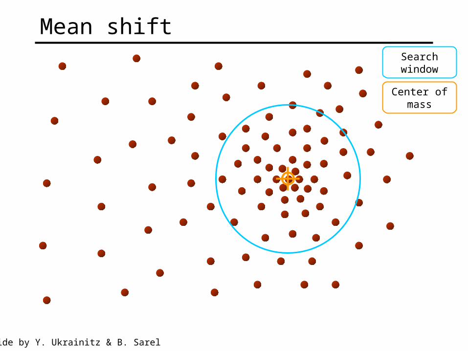
Mean shift algorithm

imageFeature space

(L*u*v* color values)

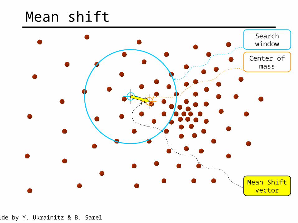
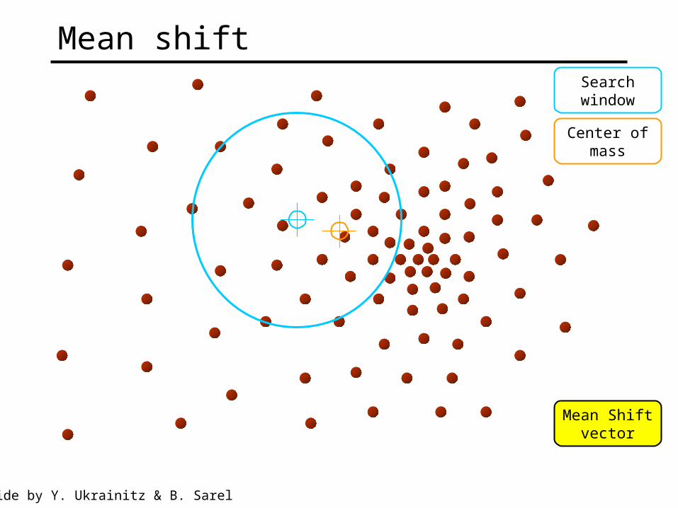
Searchwindow

Center ofmass

Mean Shiftvector

Mean shift

Slide by Y. Ukrainitz & B. Sarel

Searchwindow

Center ofmass

Mean Shiftvector

Mean shift

Slide by Y. Ukrainitz & B. Sarel

Searchwindow

Center ofmass

Mean Shiftvector

Mean shift

Slide by Y. Ukrainitz & B. Sarel

Searchwindow

Center ofmass

Mean Shiftvector

Mean shift

Slide by Y. Ukrainitz & B. Sarel

Searchwindow

Center ofmass

Mean Shiftvector

Mean shift

Slide by Y. Ukrainitz & B. Sarel

Searchwindow

Center ofmass

Mean Shiftvector

Mean shift

Slide by Y. Ukrainitz & B. Sarel

Searchwindow

Center ofmass

Mean shift

Slide by Y. Ukrainitz & B. Sarel

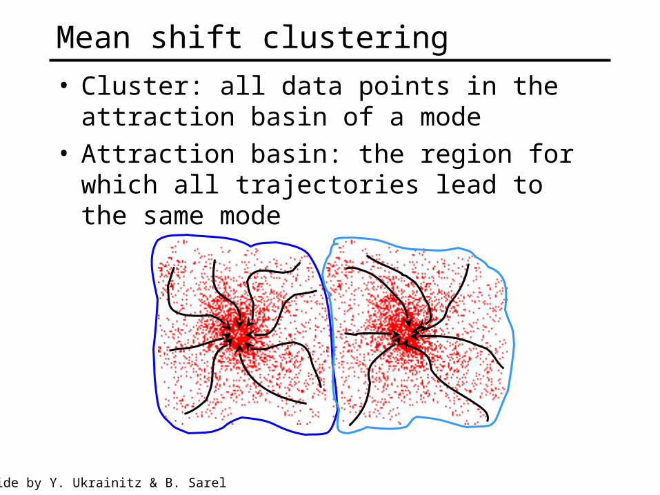
• Cluster: all data points in the attraction basin of a mode

• Attraction basin: the region for which all trajectories lead to the same mode

Mean shift clustering

Slide by Y. Ukrainitz & B. Sarel

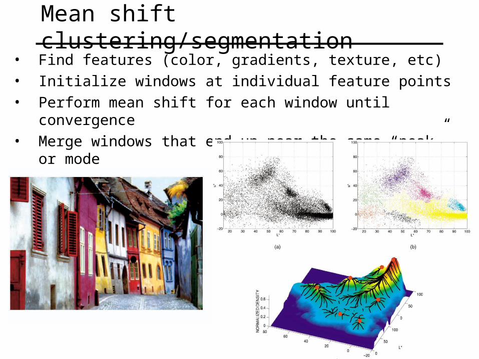
• Find features (color, gradients, texture, etc)• Initialize windows at individual feature points• Perform mean shift for each window until convergence• Merge windows that end up near the same “peak” or mode

Mean shift clustering/segmentation

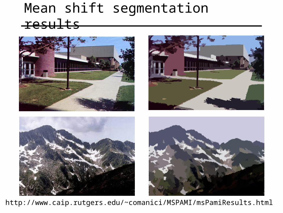
http://www.caip.rutgers.edu/~comanici/MSPAMI/msPamiResults.html

Mean shift segmentation results

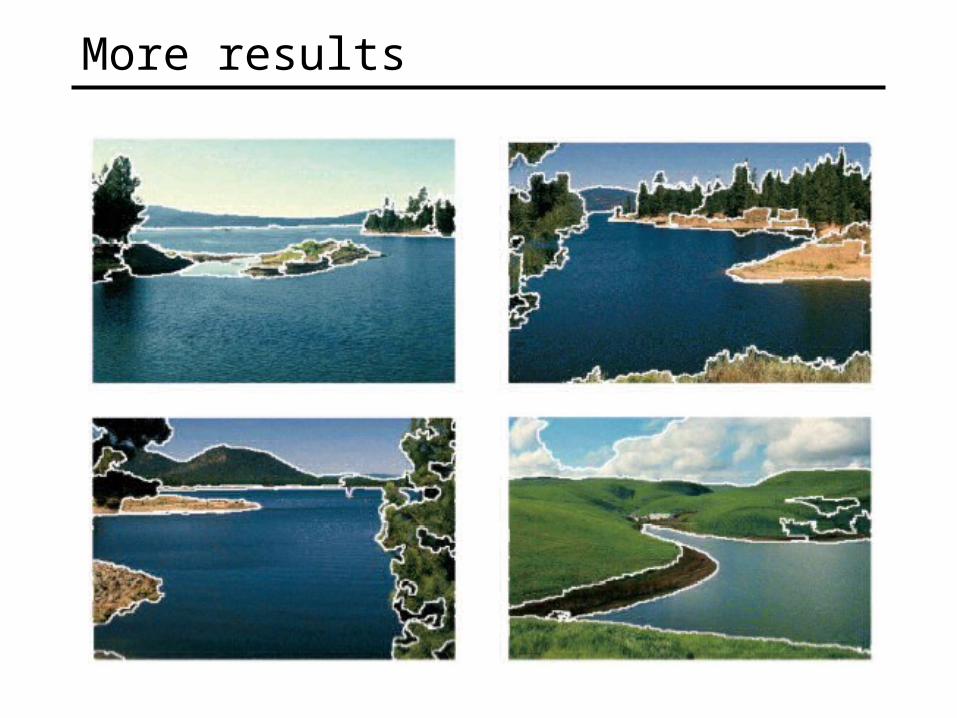
More results

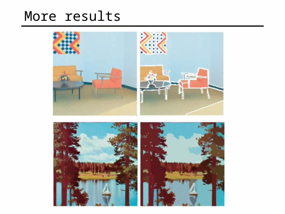
More results

Mean shift pros and cons

• Pros• Does not assume spherical clusters• Just a single parameter (window size) • Finds variable number of modes• Robust to outliers

• Cons• Output depends on window size• Computationally expensive• Does not scale well with dimension of feature space

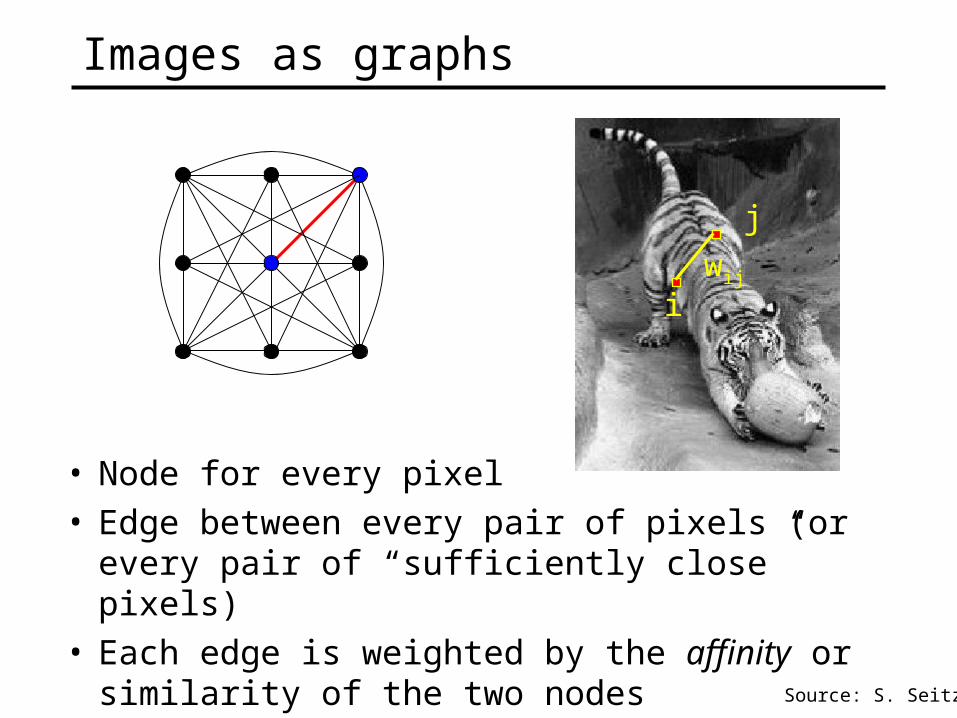
Images as graphs

• Node for every pixel• Edge between every pair of pixels (or every pair

of “sufficiently close” pixels)• Each edge is weighted by the affinity or

similarity of the two nodes

wij

i

j

Source: S. Seitz

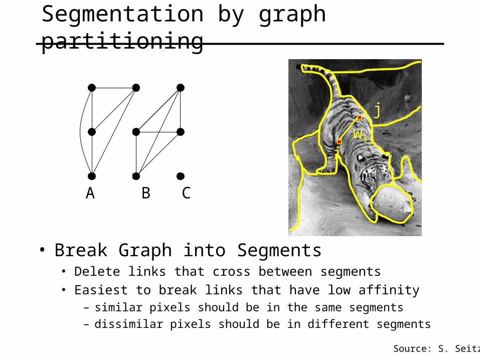
Segmentation by graph partitioning

• Break Graph into Segments• Delete links that cross between segments• Easiest to break links that have low affinity

– similar pixels should be in the same segments

– dissimilar pixels should be in different segments

A B C

Source: S. Seitz

wij

i

j

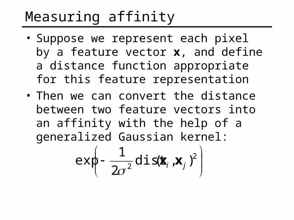
Measuring affinity

• Suppose we represent each pixel by a feature vector x, and define a distance function appropriate for this feature representation

• Then we can convert the distance between two feature vectors into an affinity with the help of a generalized Gaussian kernel:

2

2),(dist

2

1exp ji xx

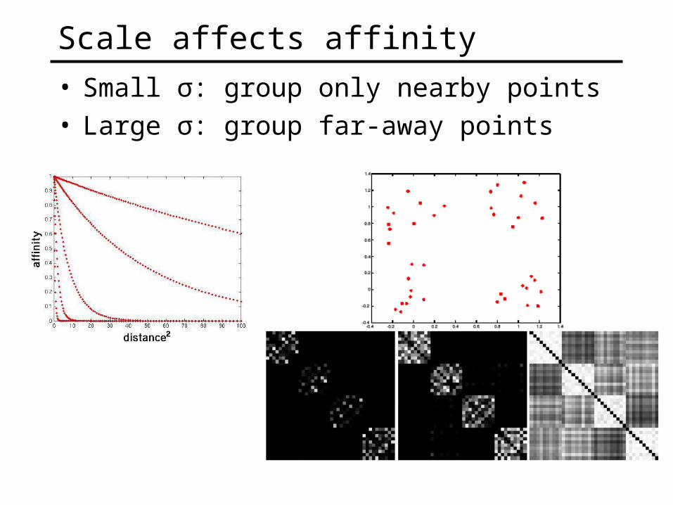
Scale affects affinity

• Small σ: group only nearby points• Large σ: group far-away points

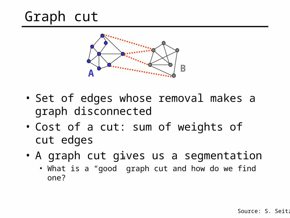
Graph cut

• Set of edges whose removal makes a graph disconnected

• Cost of a cut: sum of weights of cut edges• A graph cut gives us a segmentation

• What is a “good” graph cut and how do we find one?

A B

Source: S. Seitz

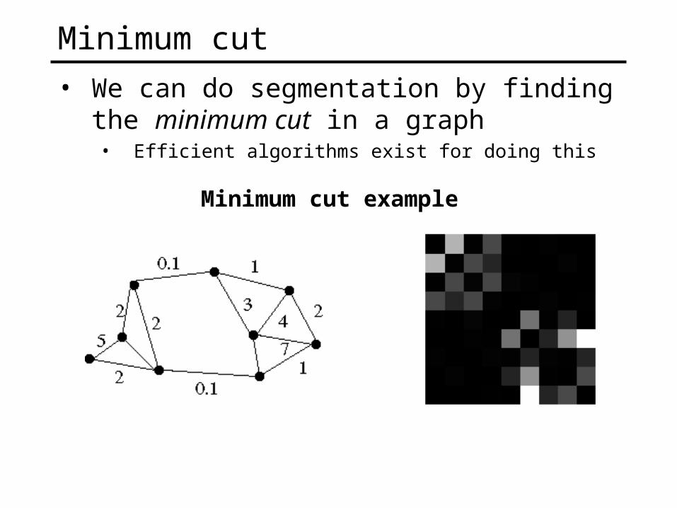
Minimum cut

• We can do segmentation by finding the minimum cut in a graph• Efficient algorithms exist for doing this

Minimum cut example

Minimum cut

• We can do segmentation by finding the minimum cut in a graph• Efficient algorithms exist for doing this

Minimum cut example

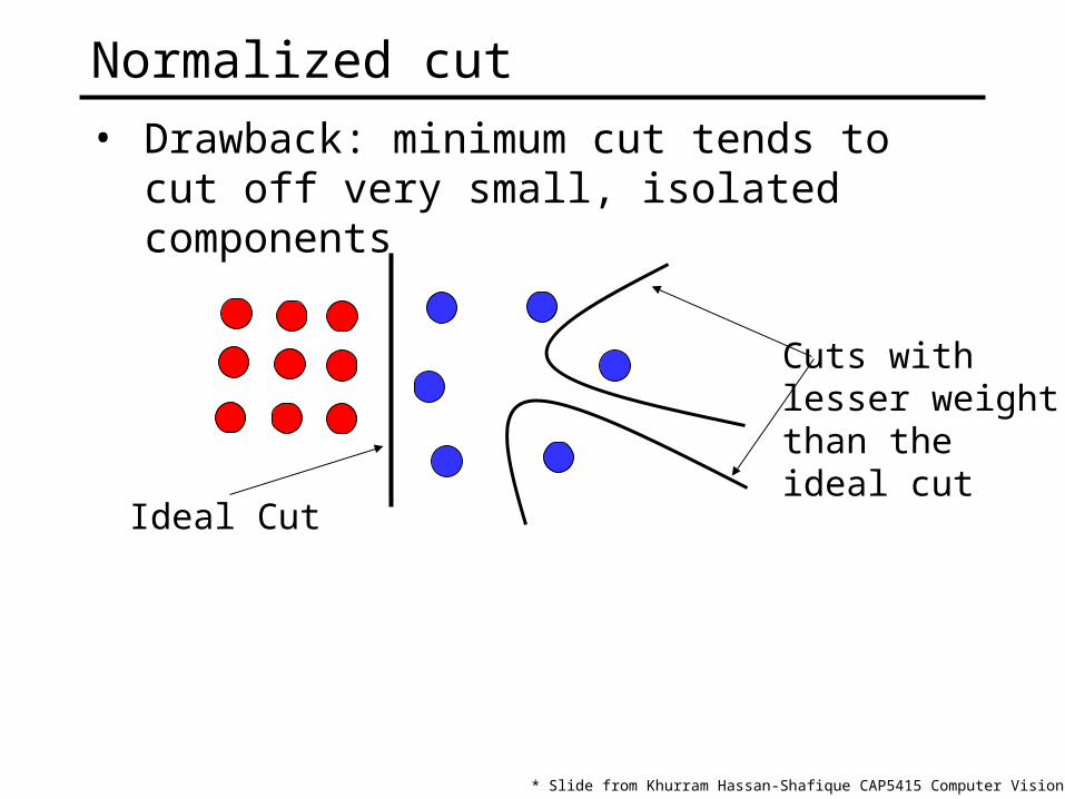
Normalized cut

• Drawback: minimum cut tends to cut off very small, isolated components

Ideal Cut

Cuts with lesser weightthan the ideal cut

* Slide from Khurram Hassan-Shafique CAP5415 Computer Vision 2003

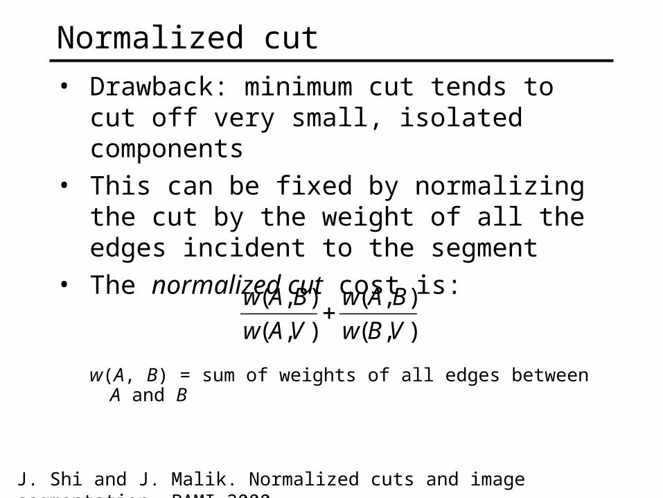
Normalized cut

• Drawback: minimum cut tends to cut off very small, isolated components

• This can be fixed by normalizing the cut by the weight of all the edges incident to the segment

• The normalized cut cost is:

w(A, B) = sum of weights of all edges between A and B

),(

),(

),(

),(

VBw

BAw

VAw

BAw

J. Shi and J. Malik. Normalized cuts and image segmentation. PAMI 2000

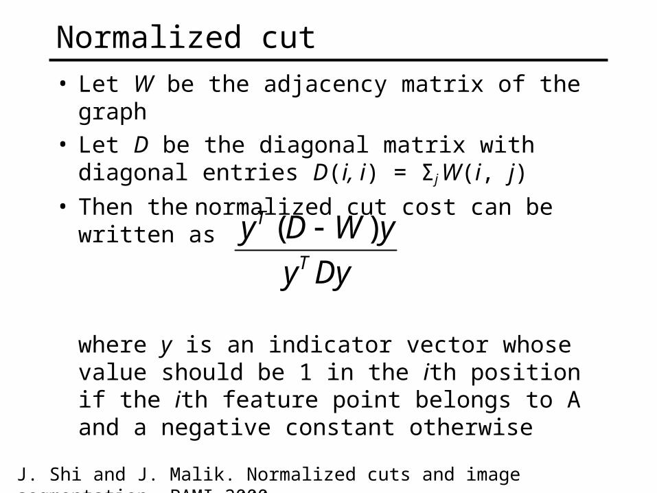
Normalized cut

• Let W be the adjacency matrix of the graph• Let D be the diagonal matrix with diagonal

entries D(i, i) = Σj W(i, j)

• Then the normalized cut cost can be written as

where y is an indicator vector whose value should be 1 in the ith position if the ith feature point belongs to A and a negative constant otherwise

J. Shi and J. Malik. Normalized cuts and image segmentation. PAMI 2000

Dyy

yWDyT

T )(

Normalized cut

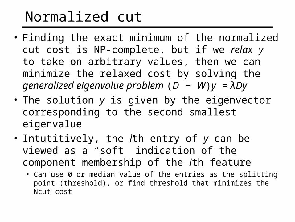
• Finding the exact minimum of the normalized cut cost is NP-complete, but if we relax y to take on arbitrary values, then we can minimize the relaxed cost by solving the generalized eigenvalue problem (D − W)y = λDy

• The solution y is given by the eigenvector corresponding to the second smallest eigenvalue

• Intutitively, the ith entry of y can be viewed as a “soft” indication of the component membership of the ith feature• Can use 0 or median value of the entries as the splitting point

(threshold), or find threshold that minimizes the Ncut cost

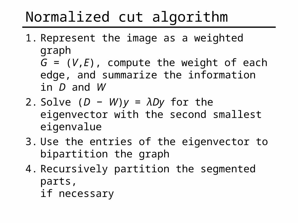
Normalized cut algorithm

1. Represent the image as a weighted graph G = (V,E), compute the weight of each edge, and summarize the information in D and W

2. Solve (D − W)y = λDy for the eigenvector with the second smallest eigenvalue

3. Use the entries of the eigenvector to bipartition the graph

4. Recursively partition the segmented parts, if necessary

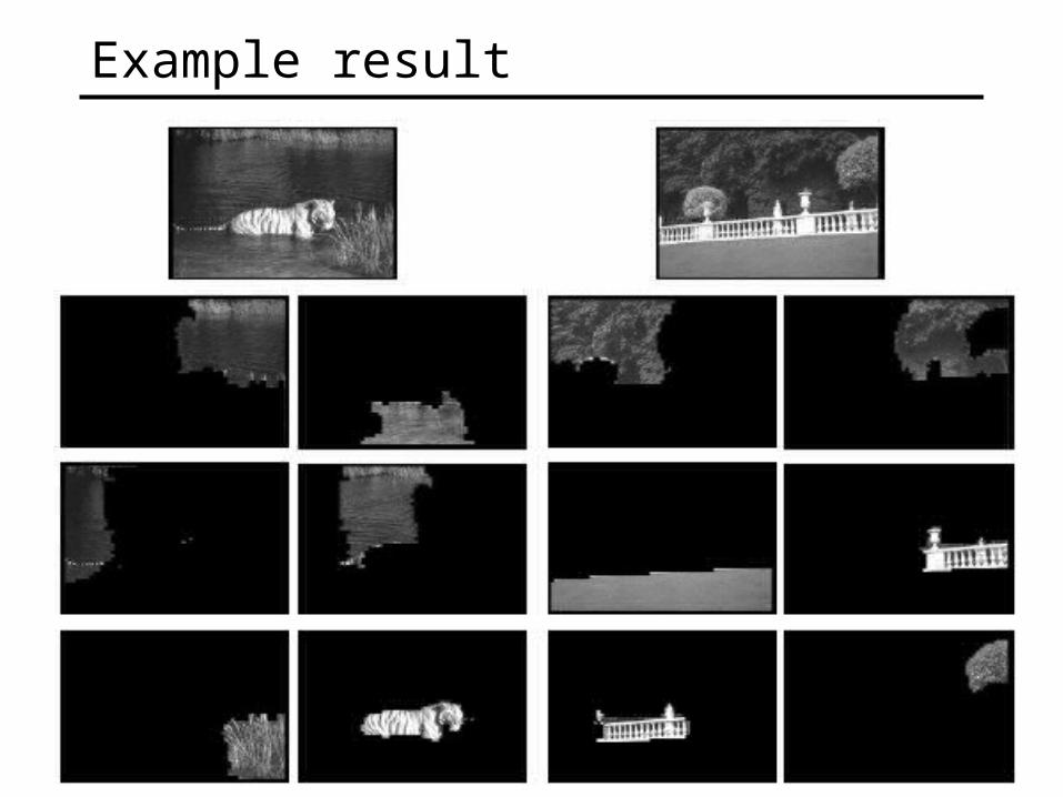
Example result

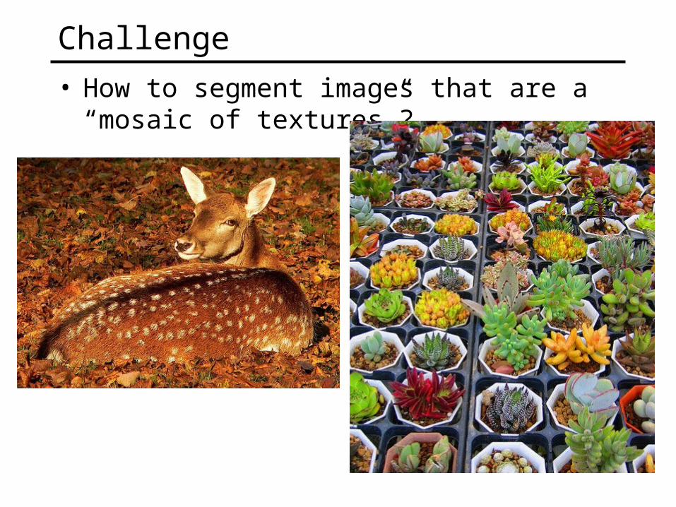
Challenge

• How to segment images that are a “mosaic of textures”?

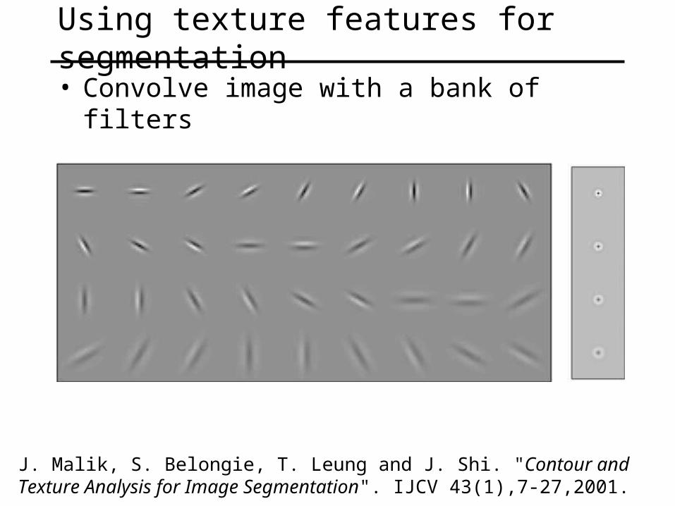
Using texture features for segmentation

• Convolve image with a bank of filters

J. Malik, S. Belongie, T. Leung and J. Shi. "Contour and Texture Analysis for Image Segmentation". IJCV 43(1),7-27,2001.

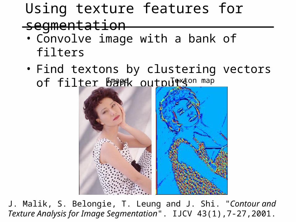
Using texture features for segmentation

• Convolve image with a bank of filters• Find textons by clustering vectors of filter bank

outputs

J. Malik, S. Belongie, T. Leung and J. Shi. "Contour and Texture Analysis for Image Segmentation". IJCV 43(1),7-27,2001.

Texton mapImage

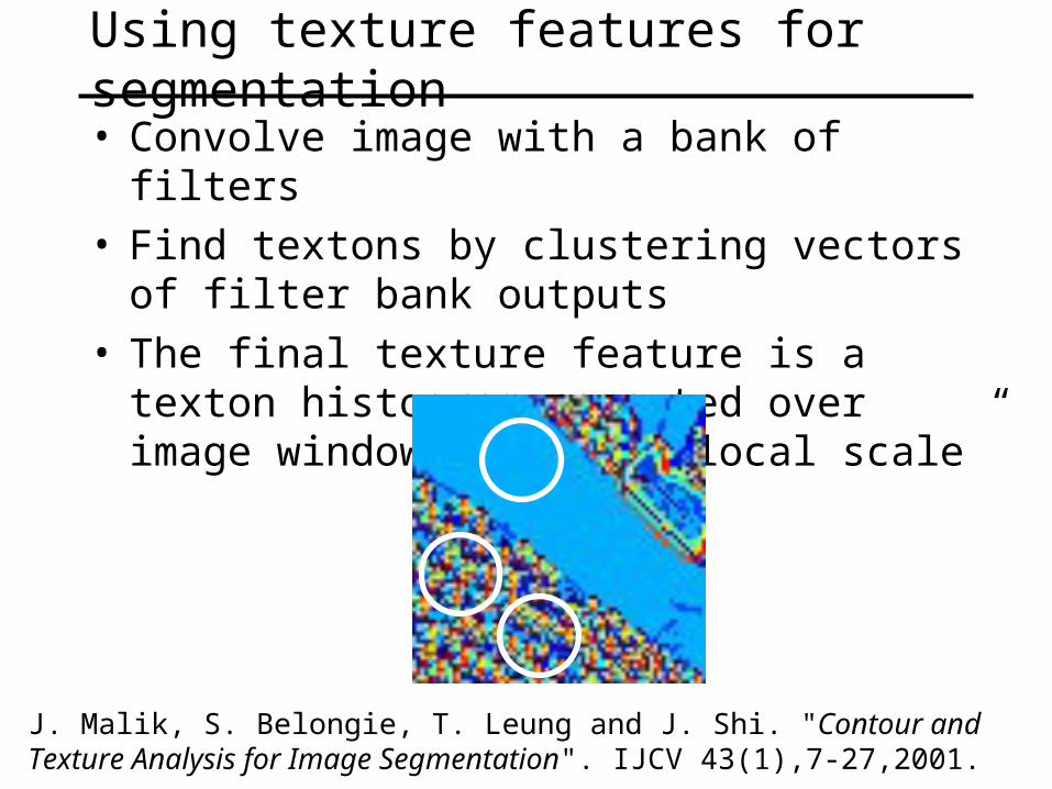
Using texture features for segmentation

• Convolve image with a bank of filters• Find textons by clustering vectors of filter bank

outputs• The final texture feature is a texton histogram

computed over image windows at some “local scale”

J. Malik, S. Belongie, T. Leung and J. Shi. "Contour and Texture Analysis for Image Segmentation". IJCV 43(1),7-27,2001.

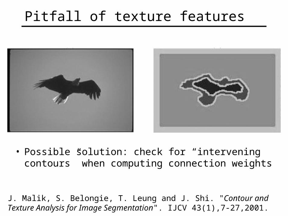
Pitfall of texture features

• Possible solution: check for “intervening contours” when computing connection weights

J. Malik, S. Belongie, T. Leung and J. Shi. "Contour and Texture Analysis for Image Segmentation". IJCV 43(1),7-27,2001.

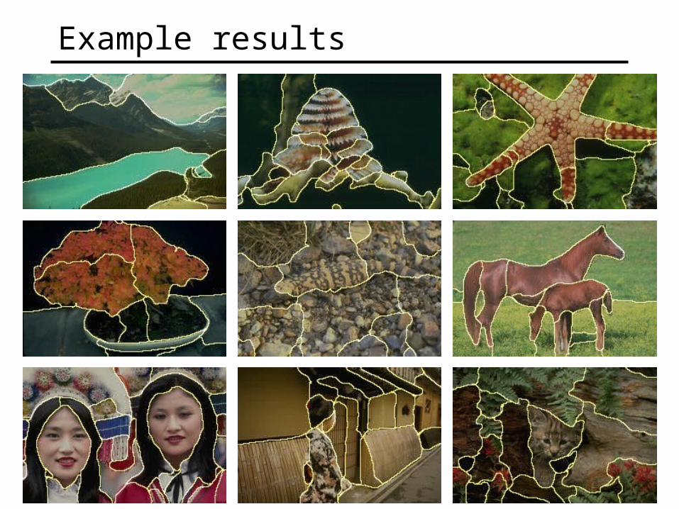
Example results

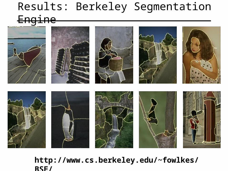
Results: Berkeley Segmentation Engine

http://www.cs.berkeley.edu/~fowlkes/BSE/

• Pros• Generic framework, can be used with many different

features and affinity formulations

• Cons• High storage requirement and time complexity• Bias towards partitioning into equal segments

Normalized cuts: Pro and con

69

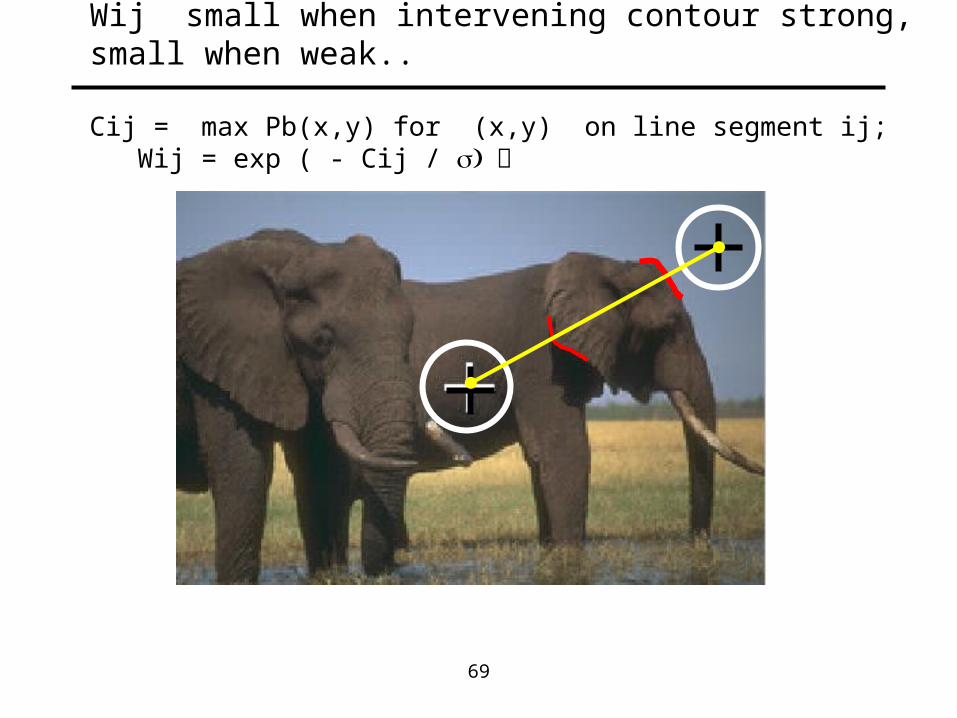
Wij small when intervening contour strong, small when weak.. Cij = max Pb(x,y) for (x,y) on line segment ij; Wij = exp ( - Cij /

70

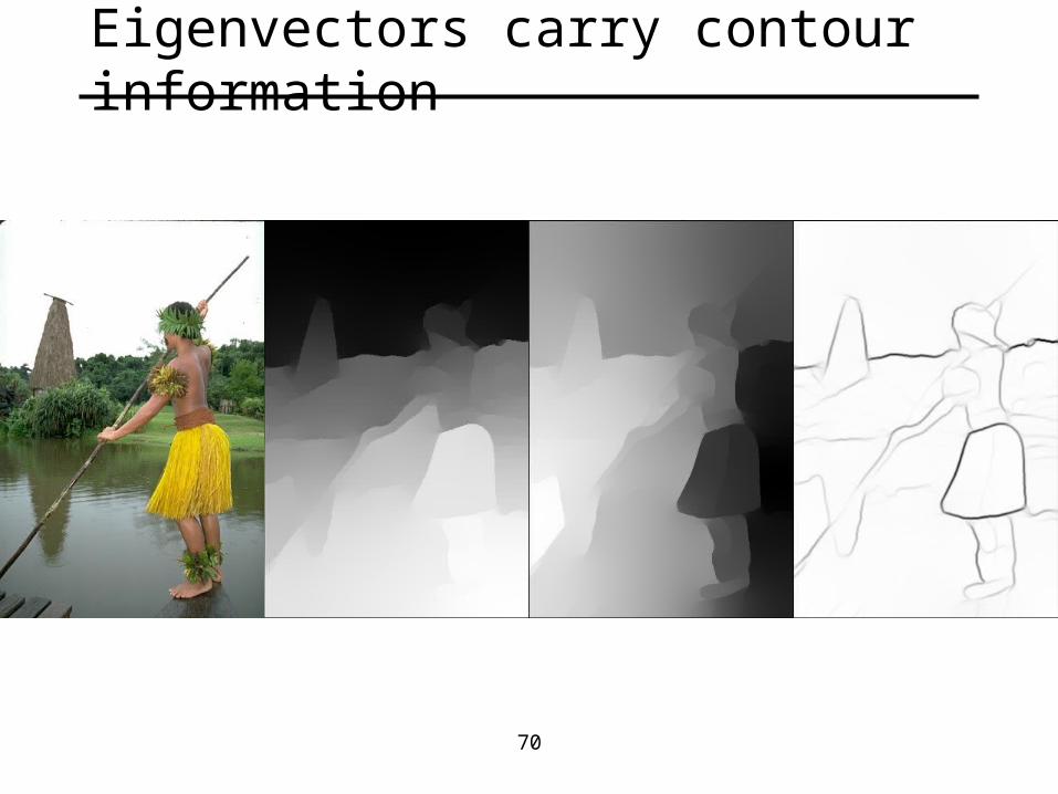
Eigenvectors carry contour information

71

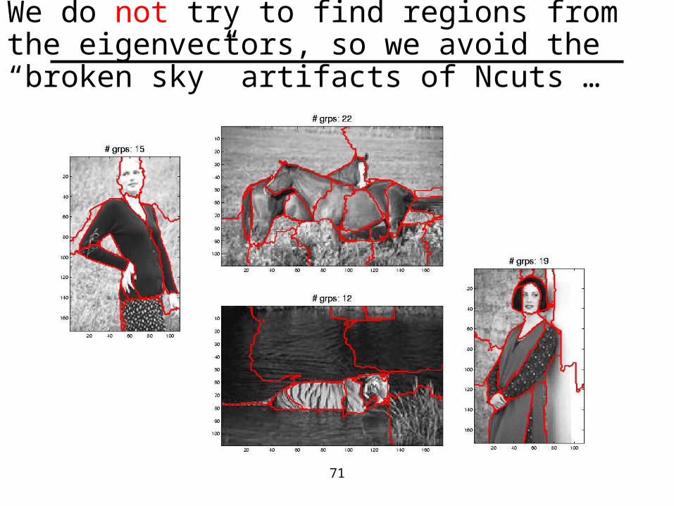
We do not try to find regions from the eigenvectors, so we avoid the “broken sky” artifacts of Ncuts …

72

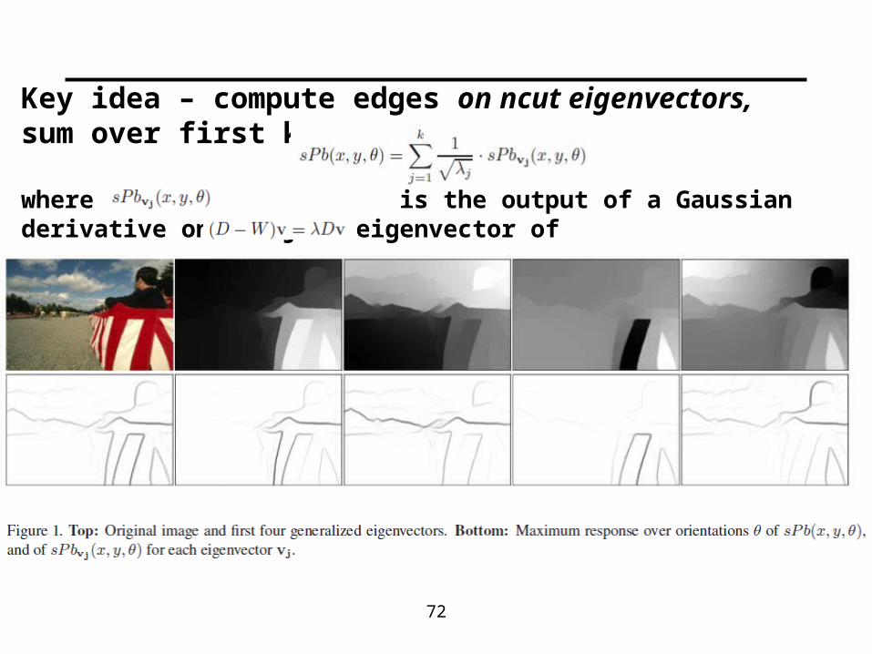
Key idea – compute edges on ncut eigenvectors, sum over first k:

where is the output of a Gaussian derivative on the j-th eigenvector of

74

Contour detection ~2008 (color)

74

Global

Slide Credits

Svetlana Lazebnik

Eamonn Keogh

Jitendra Malik