Journal of Mathematical Sciences, Vol. 193, No. 3, September, 2013

ALGORITHMS FOR LOW-DIMENSIONAL TOPOLOGY

A. Gamkrelidze UDC 515.1

Abstract. In this article, we re-introduce the so called “Arkaden–Faden–Lage” (briefly, AFL) rep-resentation of knots in three-dimensional space introduced by Kurt Reidemeister in the 1930s andshow how it can be used to develop efficient algorithms to compute some important topological knotstructures. In particular, we introduce an efficient algorithm to calculate the holonomic representationof knots introduced by V. Vassiliev and give the main ideas on how to use the AFL representations ofknots to compute the Kontsevich integral. The methods introduced here are to our knowledge noveland can open new perspectives in the development of fast algorithms in low-dimensional topology.

1. Introduction

The main goal of this article is to show how an old and forgotten idea can be analyzed and appliedin a new light to solve actual mathematical problems. As an example we use the so-called “Arkaden–Faden–Lage” (briefly, AFL) representation of knots in order to develop efficient algorithms to solve twoimportant actual problems: the holonomic description of knots and the computation of the Kontsevichintegral for knots. The idea to use the AFL representations in low-dimensional topology is publishedin [3].

The AFL representation of knots was first introduced by Kurt Reidemeister in the 1930s but didnot gain much attention maybe because the idea was only published in the German language and wasnot known to a wide community. It is a modification of the Gauss representation of knots and canhave more effective applications in practice.

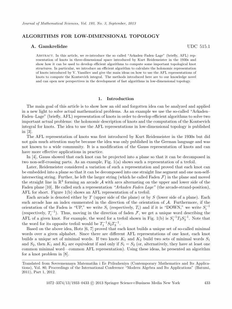
In [4], Gauss showed that each knot can be projected into a plane so that it can be decomposed intwo non-self-crossing parts. As an example, Fig. 1(a) shows such a representation of a trefoil.

Later, Reidemeister considered a variation of such a representation and proved that each knot canbe embedded into a plane so that it can be decomposed into one straight line segment and one non-self-intersecting string. Further, he left the larger string (which he called Faden F) in the plane and movedthe straight line in R

3 forming an arcade A with arcs alternating on the upper and lower side of theFaden plane [10]. He called such a representation “Arkaden Faden Lage” (the arcade-strand-position),AFL for short. Figure 1(b) shows an AFL representation of a trefoil.

Each arcade is denoted either by T (upper side of the plane) or by S (lower side of a plane). Eachsuch arcade has an index enumerated in the direction of the orientation of A. Furthermore, if theorientation of the Faden is “UP,” we write Si (respectively, Ti) and if it is “DOWN,” we write S−1

i

(respectively, T−1i ). Thus, moving in the direction of faden F , we get a unique word describing the

AFL of a given knot. For example, the word for a trefoil shown in Fig. 1(b) is S−11 T2S

−13 . Note that

the word for its opposite trefoil would be T−11 S2T

−13 .

Based on the above idea, Hotz [6, 7] proved that each knot builds a unique set of so-called minimalwords over a given alphabet. Since there are different AFL representations of one knot, each knotbuilds a unique set of minimal words. If two knots K1 and K2 build two sets of minimal words S1

and S2, then K1 and K2 are equivalent if and only if S1 = S2 (or, alternatively, they have at least onecommon minimal word—common AFL representation). Using these ideas, he presented an algorithmfor a knot problem in [8].

Translated from Sovremennaya Matematika i Ee Prilozheniya (Contemporary Mathematics and Its Applica-tions), Vol. 80, Proceedings of the International Conference “Modern Algebra and Its Applications” (Batumi,2011), Part 1, 2012.

1072–3374/13/1933–0433 c© 2013 Springer Science+Business Media New York 433

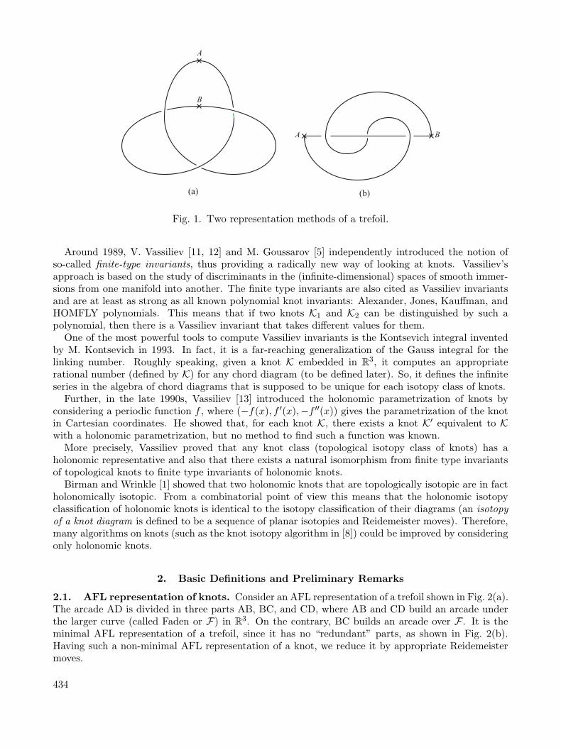
Fig. 1. Two representation methods of a trefoil.

Around 1989, V. Vassiliev [11, 12] and M. Goussarov [5] independently introduced the notion ofso-called finite-type invariants, thus providing a radically new way of looking at knots. Vassiliev’sapproach is based on the study of discriminants in the (infinite-dimensional) spaces of smooth immer-sions from one manifold into another. The finite type invariants are also cited as Vassiliev invariantsand are at least as strong as all known polynomial knot invariants: Alexander, Jones, Kauffman, andHOMFLY polynomials. This means that if two knots K1 and K2 can be distinguished by such apolynomial, then there is a Vassiliev invariant that takes different values for them.

One of the most powerful tools to compute Vassiliev invariants is the Kontsevich integral inventedby M. Kontsevich in 1993. In fact, it is a far-reaching generalization of the Gauss integral for thelinking number. Roughly speaking, given a knot K embedded in R

3, it computes an appropriaterational number (defined by K) for any chord diagram (to be defined later). So, it defines the infiniteseries in the algebra of chord diagrams that is supposed to be unique for each isotopy class of knots.

Further, in the late 1990s, Vassiliev [13] introduced the holonomic parametrization of knots byconsidering a periodic function f , where (−f(x), f ′(x),−f ′′(x)) gives the parametrization of the knotin Cartesian coordinates. He showed that, for each knot K, there exists a knot K′ equivalent to Kwith a holonomic parametrization, but no method to find such a function was known.

More precisely, Vassiliev proved that any knot class (topological isotopy class of knots) has aholonomic representative and also that there exists a natural isomorphism from finite type invariantsof topological knots to finite type invariants of holonomic knots.

Birman and Wrinkle [1] showed that two holonomic knots that are topologically isotopic are in factholonomically isotopic. From a combinatorial point of view this means that the holonomic isotopyclassification of holonomic knots is identical to the isotopy classification of their diagrams (an isotopyof a knot diagram is defined to be a sequence of planar isotopies and Reidemeister moves). Therefore,many algorithms on knots (such as the knot isotopy algorithm in [8]) could be improved by consideringonly holonomic knots.

2. Basic Definitions and Preliminary Remarks

2.1. AFL representation of knots. Consider an AFL representation of a trefoil shown in Fig. 2(a).The arcade AD is divided in three parts AB, BC, and CD, where AB and CD build an arcade underthe larger curve (called Faden or F) in R

3. On the contrary, BC builds an arcade over F . It is theminimal AFL representation of a trefoil, since it has no “redundant” parts, as shown in Fig. 2(b).Having such a non-minimal AFL representation of a knot, we reduce it by appropriate Reidemeistermoves.

434

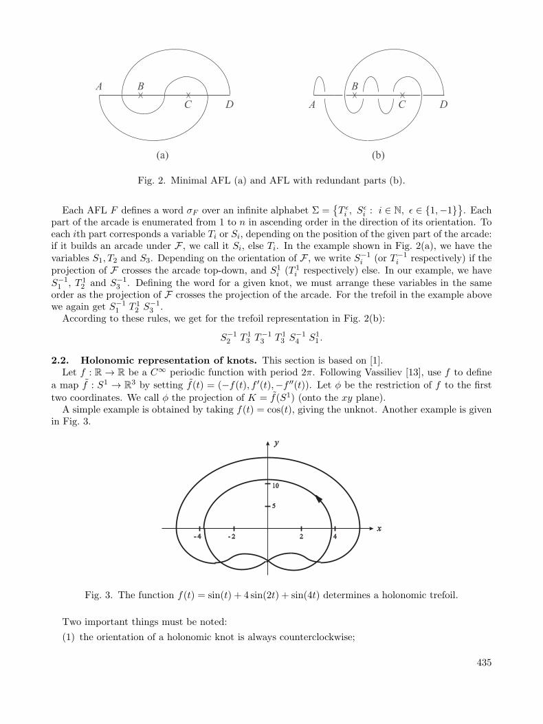
Fig. 2. Minimal AFL (a) and AFL with redundant parts (b).

Each AFL F defines a word σF over an infinite alphabet Σ ={T εi , Sε

i : i ∈ N, ε ∈ {1,−1}}. Each

part of the arcade is enumerated from 1 to n in ascending order in the direction of its orientation. Toeach ith part corresponds a variable Ti or Si, depending on the position of the given part of the arcade:if it builds an arcade under F , we call it Si, else Ti. In the example shown in Fig. 2(a), we have thevariables S1, T2 and S3. Depending on the orientation of F , we write S−1

i (or T−1i respectively) if the

projection of F crosses the arcade top-down, and S1i (T 1

i respectively) else. In our example, we have

S−11 , T 1

2 and S−13 . Defining the word for a given knot, we must arrange these variables in the same

order as the projection of F crosses the projection of the arcade. For the trefoil in the example abovewe again get S−1

1 T 12 S−1

3 .According to these rules, we get for the trefoil representation in Fig. 2(b):

S−12 T 1

3 T−13 T 1

3 S−14 S1

1 .

2.2. Holonomic representation of knots. This section is based on [1].Let f : R → R be a C∞ periodic function with period 2π. Following Vassiliev [13], use f to define

a map f : S1 → R3 by setting f(t) = (−f(t), f ′(t),−f ′′(t)). Let φ be the restriction of f to the first

two coordinates. We call φ the projection of K = f(S1) (onto the xy plane).A simple example is obtained by taking f(t) = cos(t), giving the unknot. Another example is given

in Fig. 3.

Fig. 3. The function f(t) = sin(t) + 4 sin(2t) + sin(4t) determines a holonomic trefoil.

Two important things must be noted:

(1) the orientation of a holonomic knot is always counterclockwise;

435

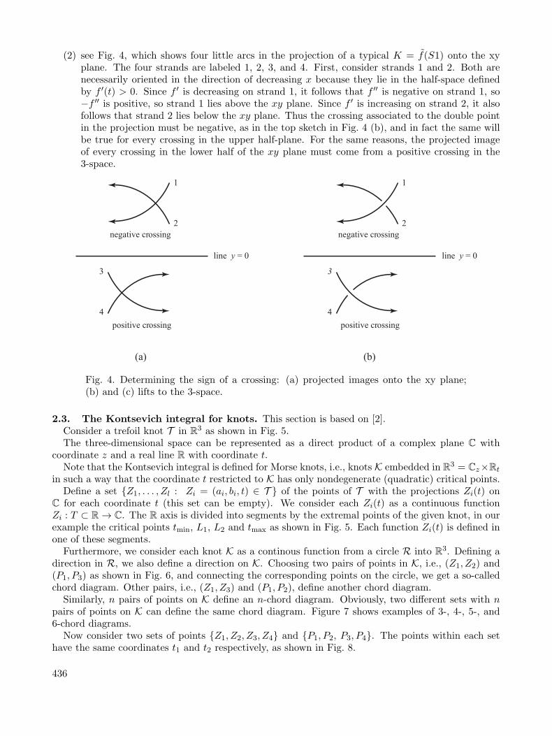
(2) see Fig. 4, which shows four little arcs in the projection of a typical K = f(S1) onto the xyplane. The four strands are labeled 1, 2, 3, and 4. First, consider strands 1 and 2. Both arenecessarily oriented in the direction of decreasing x because they lie in the half-space definedby f ′(t) > 0. Since f ′ is decreasing on strand 1, it follows that f ′′ is negative on strand 1, so−f ′′ is positive, so strand 1 lies above the xy plane. Since f ′ is increasing on strand 2, it alsofollows that strand 2 lies below the xy plane. Thus the crossing associated to the double pointin the projection must be negative, as in the top sketch in Fig. 4 (b), and in fact the same willbe true for every crossing in the upper half-plane. For the same reasons, the projected imageof every crossing in the lower half of the xy plane must come from a positive crossing in the3-space.

Fig. 4. Determining the sign of a crossing: (a) projected images onto the xy plane;(b) and (c) lifts to the 3-space.

2.3. The Kontsevich integral for knots. This section is based on [2].Consider a trefoil knot T in R

3 as shown in Fig. 5.The three-dimensional space can be represented as a direct product of a complex plane C with

coordinate z and a real line R with coordinate t.Note that the Kontsevich integral is defined for Morse knots, i.e., knots K embedded in R

3 = Cz×Rt

in such a way that the coordinate t restricted to K has only nondegenerate (quadratic) critical points.Define a set {Z1, . . . , Zl : Zi = (ai, bi, t) ∈ T } of the points of T with the projections Zi(t) on

C for each coordinate t (this set can be empty). We consider each Zi(t) as a continuous functionZi : T ⊂ R → C. The R axis is divided into segments by the extremal points of the given knot, in ourexample the critical points tmin, L1, L2 and tmax as shown in Fig. 5. Each function Zi(t) is defined inone of these segments.

Furthermore, we consider each knot K as a continous function from a circle R into R3. Defining a

direction in R, we also define a direction on K. Choosing two pairs of points in K, i.e., (Z1, Z2) and(P1, P3) as shown in Fig. 6, and connecting the corresponding points on the circle, we get a so-calledchord diagram. Other pairs, i.e., (Z1, Z3) and (P1, P2), define another chord diagram.

Similarly, n pairs of points on K define an n-chord diagram. Obviously, two different sets with npairs of points on K can define the same chord diagram. Figure 7 shows examples of 3-, 4-, 5-, and6-chord diagrams.

Now consider two sets of points {Z1, Z2, Z3, Z4} and {P1, P2, P3, P4}. The points within each sethave the same coordinates t1 and t2 respectively, as shown in Fig. 8.

436

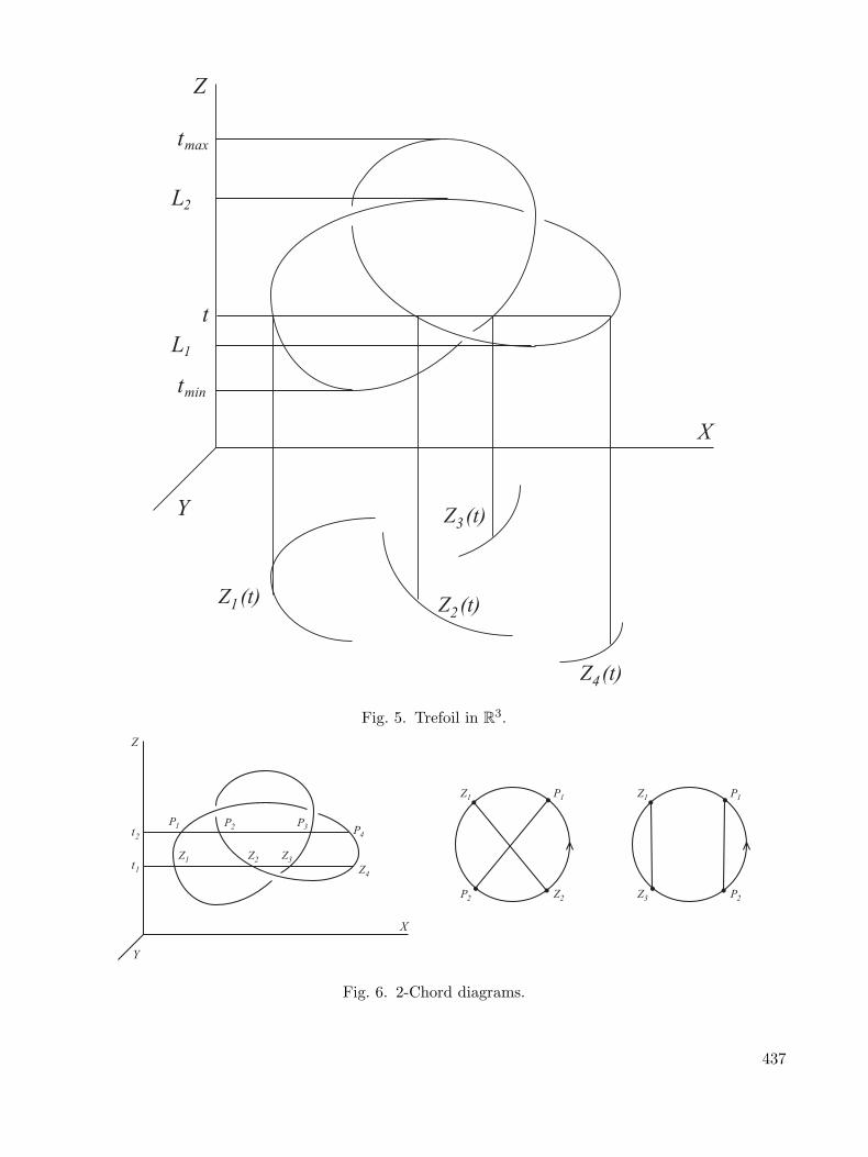
Fig. 5. Trefoil in R3.

Fig. 6. 2-Chord diagrams.

437

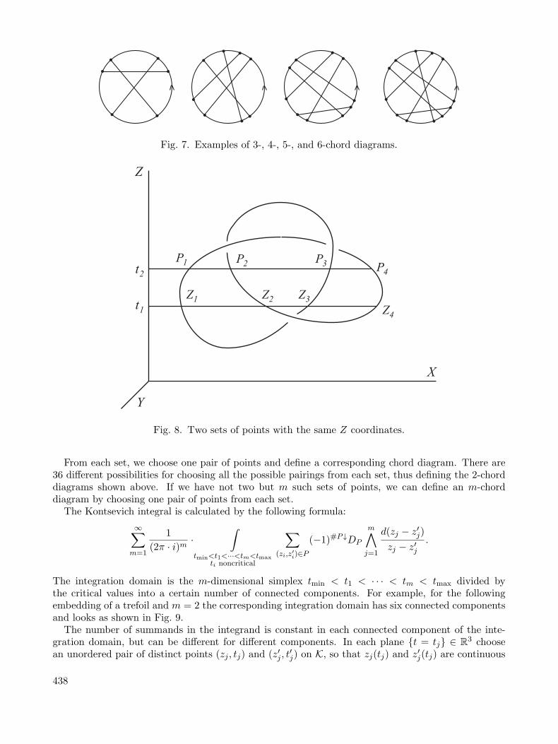
Fig. 7. Examples of 3-, 4-, 5-, and 6-chord diagrams.

Fig. 8. Two sets of points with the same Z coordinates.

From each set, we choose one pair of points and define a corresponding chord diagram. There are36 different possibilities for choosing all the possible pairings from each set, thus defining the 2-chorddiagrams shown above. If we have not two but m such sets of points, we can define an m-chorddiagram by choosing one pair of points from each set.

The Kontsevich integral is calculated by the following formula:

∞∑

m=1

1

(2π · i)m ·∫

tmin<t1<···<tm<tmaxti noncritical

∑

(zi,z′i)∈P(−1)#P↓DP

m∧

j=1

d(zj − z′j)zj − z′j

.

The integration domain is the m-dimensional simplex tmin < t1 < · · · < tm < tmax divided bythe critical values into a certain number of connected components. For example, for the followingembedding of a trefoil and m = 2 the corresponding integration domain has six connected componentsand looks as shown in Fig. 9.

The number of summands in the integrand is constant in each connected component of the inte-gration domain, but can be different for different components. In each plane {t = tj} ∈ R

3 choosean unordered pair of distinct points (zj , tj) and (z′j , t

′j) on K, so that zj(tj) and z′j(tj) are continuous

438

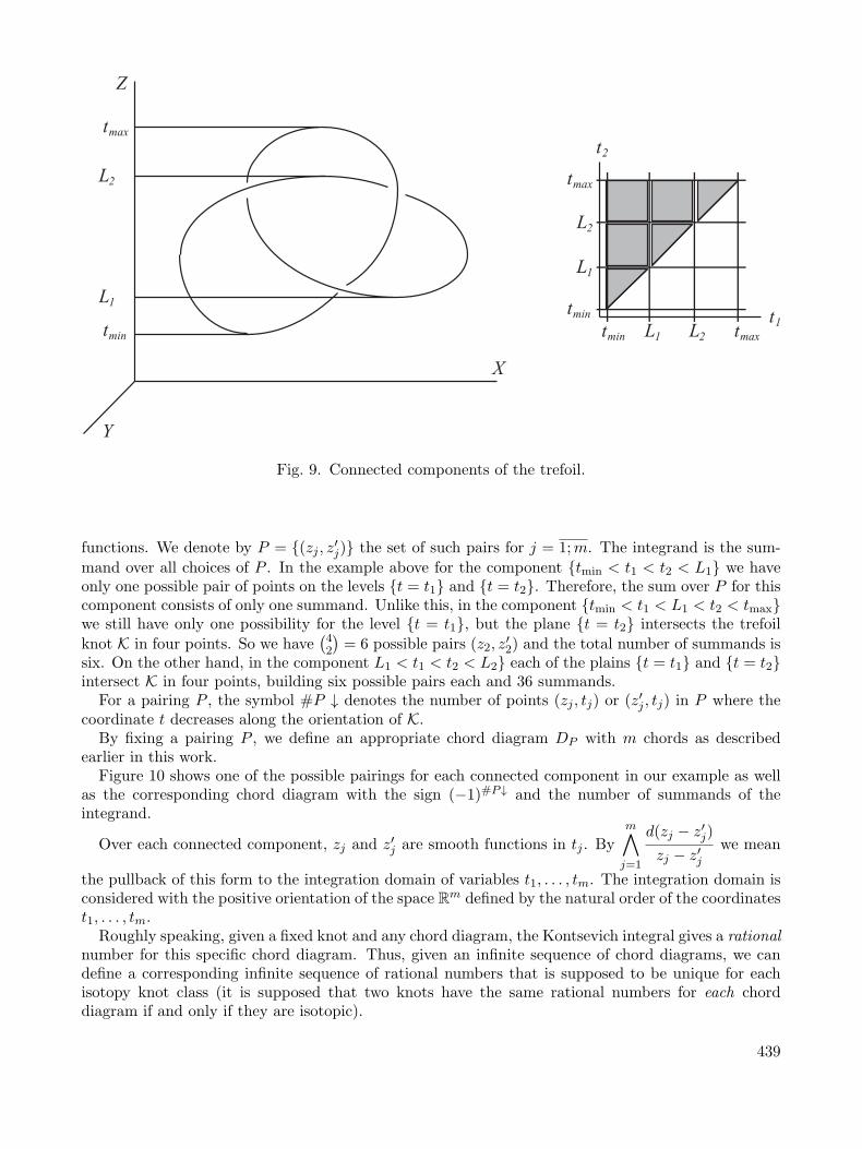
Fig. 9. Connected components of the trefoil.

functions. We denote by P = {(zj , z′j)} the set of such pairs for j = 1;m. The integrand is the sum-

mand over all choices of P . In the example above for the component {tmin < t1 < t2 < L1} we haveonly one possible pair of points on the levels {t = t1} and {t = t2}. Therefore, the sum over P for thiscomponent consists of only one summand. Unlike this, in the component {tmin < t1 < L1 < t2 < tmax}we still have only one possibility for the level {t = t1}, but the plane {t = t2} intersects the trefoil

knot K in four points. So we have(42

)= 6 possible pairs (z2, z

′2) and the total number of summands is

six. On the other hand, in the component L1 < t1 < t2 < L2} each of the plains {t = t1} and {t = t2}intersect K in four points, building six possible pairs each and 36 summands.

For a pairing P , the symbol #P ↓ denotes the number of points (zj , tj) or (z′j , tj) in P where thecoordinate t decreases along the orientation of K.

By fixing a pairing P , we define an appropriate chord diagram DP with m chords as describedearlier in this work.

Figure 10 shows one of the possible pairings for each connected component in our example as wellas the corresponding chord diagram with the sign (−1)#P↓ and the number of summands of theintegrand.

Over each connected component, zj and z′j are smooth functions in tj . By

m∧

j=1

d(zj − z′j)zj − z′j

we mean

the pullback of this form to the integration domain of variables t1, . . . , tm. The integration domain isconsidered with the positive orientation of the space Rm defined by the natural order of the coordinatest1, . . . , tm.

Roughly speaking, given a fixed knot and any chord diagram, the Kontsevich integral gives a rationalnumber for this specific chord diagram. Thus, given an infinite sequence of chord diagrams, we candefine a corresponding infinite sequence of rational numbers that is supposed to be unique for eachisotopy knot class (it is supposed that two knots have the same rational numbers for each chorddiagram if and only if they are isotopic).

439

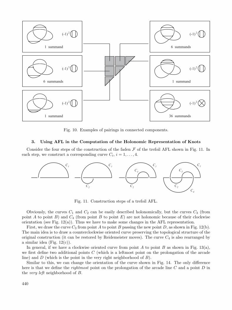
Fig. 10. Examples of pairings in connected components.

3. Using AFL in the Computation of the Holonomic Representation of Knots

Consider the four steps of the construction of the faden F of the trefoil AFL shown in Fig. 11. Ineach step, we construct a corresponding curve Ci, i = 1, . . . , 4.

Fig. 11. Construction steps of a trefoil AFL.

Obviously, the curves C1 and C2 can be easily described holonomically, but the curves C3 (frompoint A to point B) and C4 (from point B to point E) are not holonomic because of their clockwiseorientation (see Fig. 12(a)). Thus we have to make some changes in the AFL representation.

First, we draw the curve C3 from point A to point B passing the new pointD, as shown in Fig. 12(b).The main idea is to draw a counterclockwise oriented curve preserving the topological structure of theoriginal construction (it can be restored by Reidemeister moves). The curve C4 is also rearranged bya similar idea (Fig. 12(c)).

In general, if we have a clockwise oriented curve from point A to point B as shown in Fig. 13(a),we first define two additional points C (which is a leftmost point on the prolongation of the arcadeline) and D (which is the point in the very right neighborhood of B).

Similar to this, we can change the orientation of the curve shown in Fig. 14. The only differencehere is that we define the rightmost point on the prolongation of the arcade line C and a point D inthe very left neighborhood of B.

440

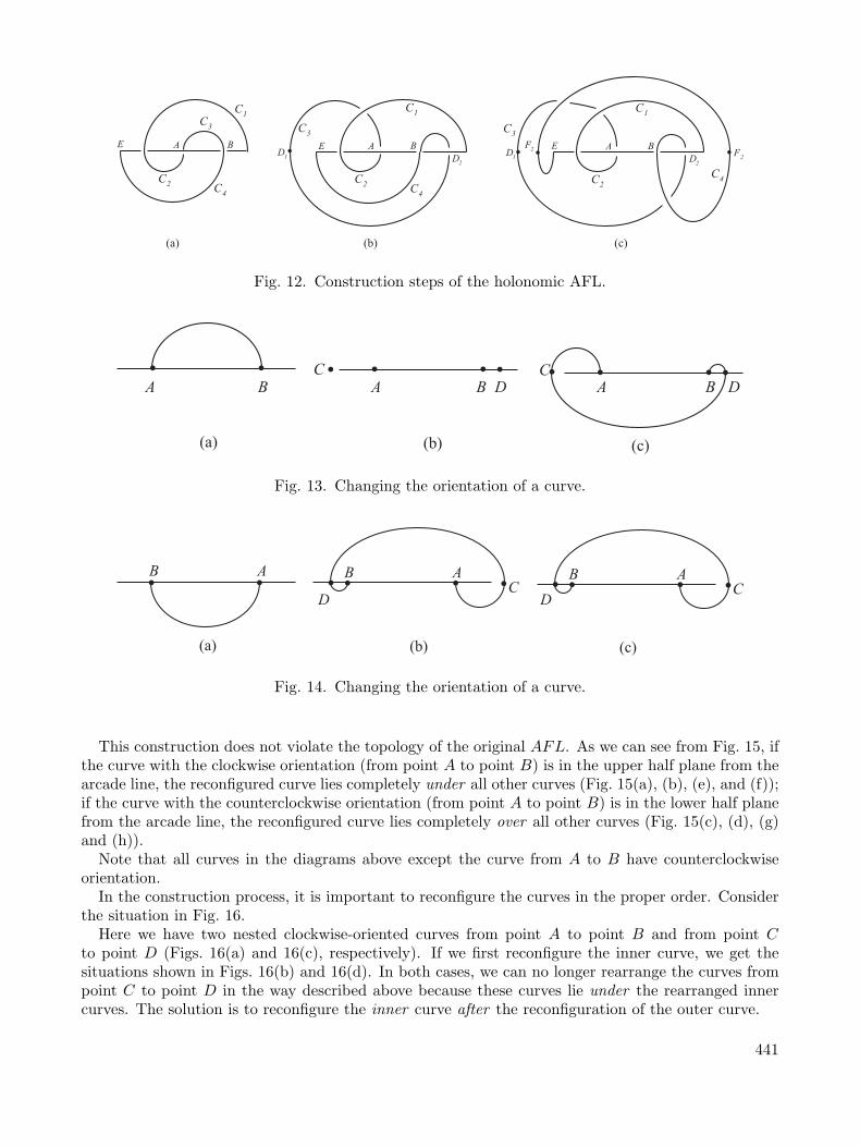
Fig. 12. Construction steps of the holonomic AFL.

Fig. 13. Changing the orientation of a curve.

Fig. 14. Changing the orientation of a curve.

This construction does not violate the topology of the original AFL. As we can see from Fig. 15, ifthe curve with the clockwise orientation (from point A to point B) is in the upper half plane from thearcade line, the reconfigured curve lies completely under all other curves (Fig. 15(a), (b), (e), and (f));if the curve with the counterclockwise orientation (from point A to point B) is in the lower half planefrom the arcade line, the reconfigured curve lies completely over all other curves (Fig. 15(c), (d), (g)and (h)).

Note that all curves in the diagrams above except the curve from A to B have counterclockwiseorientation.

In the construction process, it is important to reconfigure the curves in the proper order. Considerthe situation in Fig. 16.

Here we have two nested clockwise-oriented curves from point A to point B and from point Cto point D (Figs. 16(a) and 16(c), respectively). If we first reconfigure the inner curve, we get thesituations shown in Figs. 16(b) and 16(d). In both cases, we can no longer rearrange the curves frompoint C to point D in the way described above because these curves lie under the rearranged innercurves. The solution is to reconfigure the inner curve after the reconfiguration of the outer curve.

441

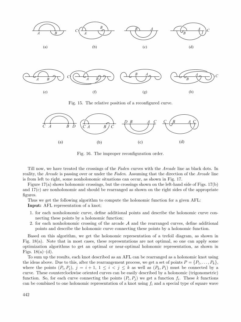
Fig. 15. The relative position of a reconfigured curve.

Fig. 16. The improper reconfiguration order.

Till now, we have treated the crossings of the Faden curves with the Arcade line as black dots. Inreality, the Arcade is passing over or under the Faden. Assuming that the direction of the Arcade lineis from left to right, some nonholonomic situations can occur, as shown in Fig. 17.

Figure 17(a) shows holonomic crossings, but the crossings shown on the left-hand side of Figs. 17(b)and 17(c) are nonholonomic and should be rearranged as shown on the right sides of the appropriatefigures.

Thus we get the following algorithm to compute the holonomic function for a given AFL:Input: AFL representation of a knot;

1. for each nonholonomic curve, define additional points and describe the holonomic curve con-necting these points by a holonomic function;

2. for each nonholonomic crossing of the arcade A and the rearranged curves, define additionalpoints and describe the holonomic curve connecting these points by a holonomic function.

Based on this algorithm, we get the holonomic representation of a trefoil diagram, as shown inFig. 18(a). Note that in most cases, these representations are not optimal, so one can apply someoptimization algorithms to get an optimal or near-optimal holonomic representation, as shown inFigs. 18(a)–(d).

To sum up the results, each knot described as an AFL can be rearranged as a holonomic knot usingthe ideas above. Due to this, after the rearrangement process, we get a set of points P = {P1, . . . , Pk},where the points (Pi, Pj), j = i + 1, 1 ≤ i < j ≤ k as well as (Pk, P1) must be connected by acurve. These counterclockwise oriented curves can be easily described by a holonomic (trigonometric)function. So, for each curve connecting the points (Pi, Pj) we get a function fi. These k functionscan be combined to one holonomic representation of a knot using fi and a special type of square wave

442

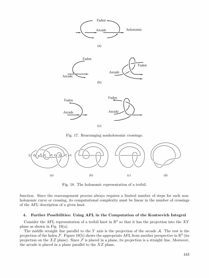
Fig. 17. Rearranging nonholonomic crossings.

Fig. 18. The holonomic representation of a trefoil.

function. Since the rearrangement process always requires a limited number of steps for each non-holonomic curve or crossing, its computational complexity must be linear in the number of crossingsof the AFL description of a given knot.

4. Further Possibilities: Using AFL in the Computation of the Kontsevich Integral

Consider the AFL representation of a trefoil knot in R3 so that it has the projection into the XY

plane as shown in Fig. 19(a).The middle straight line parallel to the Y axis is the projection of the arcade A. The rest is the

projection of the faden F . Figure 19(b) shows the appropriate AFL from another perspective in R3 (its

projection on the XZ plane). Since F is placed in a plane, its projection is a straight line. Moreover,the arcade is placed in a plane parallel to the XZ plane.

443

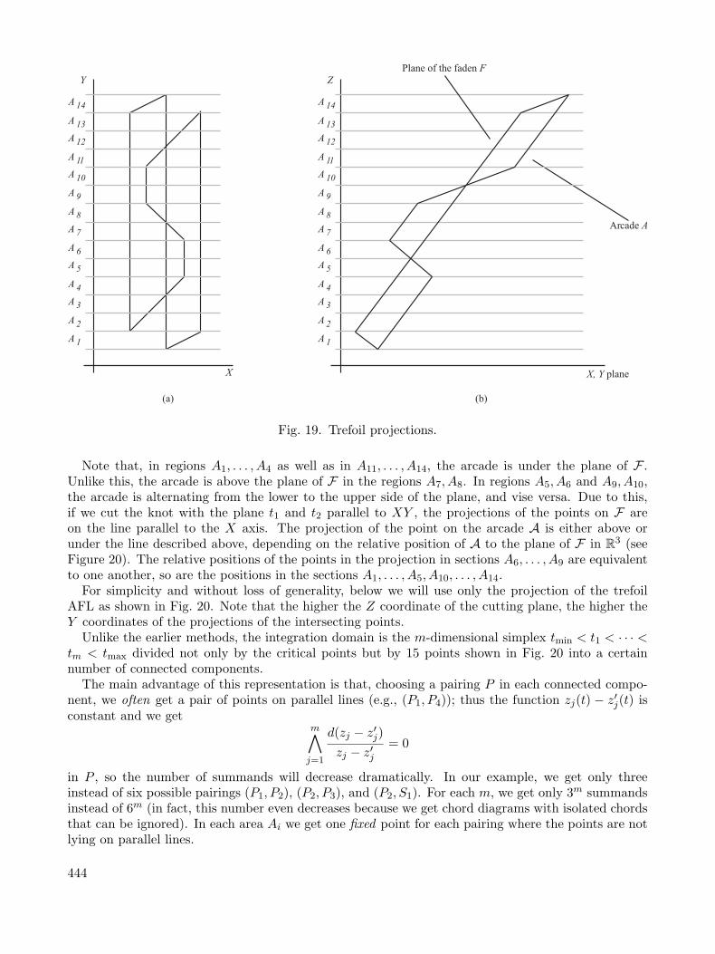
Fig. 19. Trefoil projections.

Note that, in regions A1, . . . , A4 as well as in A11, . . . , A14, the arcade is under the plane of F .Unlike this, the arcade is above the plane of F in the regions A7, A8. In regions A5, A6 and A9, A10,the arcade is alternating from the lower to the upper side of the plane, and vise versa. Due to this,if we cut the knot with the plane t1 and t2 parallel to XY , the projections of the points on F areon the line parallel to the X axis. The projection of the point on the arcade A is either above orunder the line described above, depending on the relative position of A to the plane of F in R

3 (seeFigure 20). The relative positions of the points in the projection in sections A6, . . . , A9 are equivalentto one another, so are the positions in the sections A1, . . . , A5, A10, . . . , A14.

For simplicity and without loss of generality, below we will use only the projection of the trefoilAFL as shown in Fig. 20. Note that the higher the Z coordinate of the cutting plane, the higher theY coordinates of the projections of the intersecting points.

Unlike the earlier methods, the integration domain is the m-dimensional simplex tmin < t1 < · · · <tm < tmax divided not only by the critical points but by 15 points shown in Fig. 20 into a certainnumber of connected components.

The main advantage of this representation is that, choosing a pairing P in each connected compo-nent, we often get a pair of points on parallel lines (e.g., (P1, P4)); thus the function zj(t) − z′j(t) isconstant and we get

m∧

j=1

d(zj − z′j)zj − z′j

= 0

in P , so the number of summands will decrease dramatically. In our example, we get only threeinstead of six possible pairings (P1, P2), (P2, P3), and (P2, S1). For each m, we get only 3m summandsinstead of 6m (in fact, this number even decreases because we get chord diagrams with isolated chordsthat can be ignored). In each area Ai we get one fixed point for each pairing where the points are notlying on parallel lines.

444

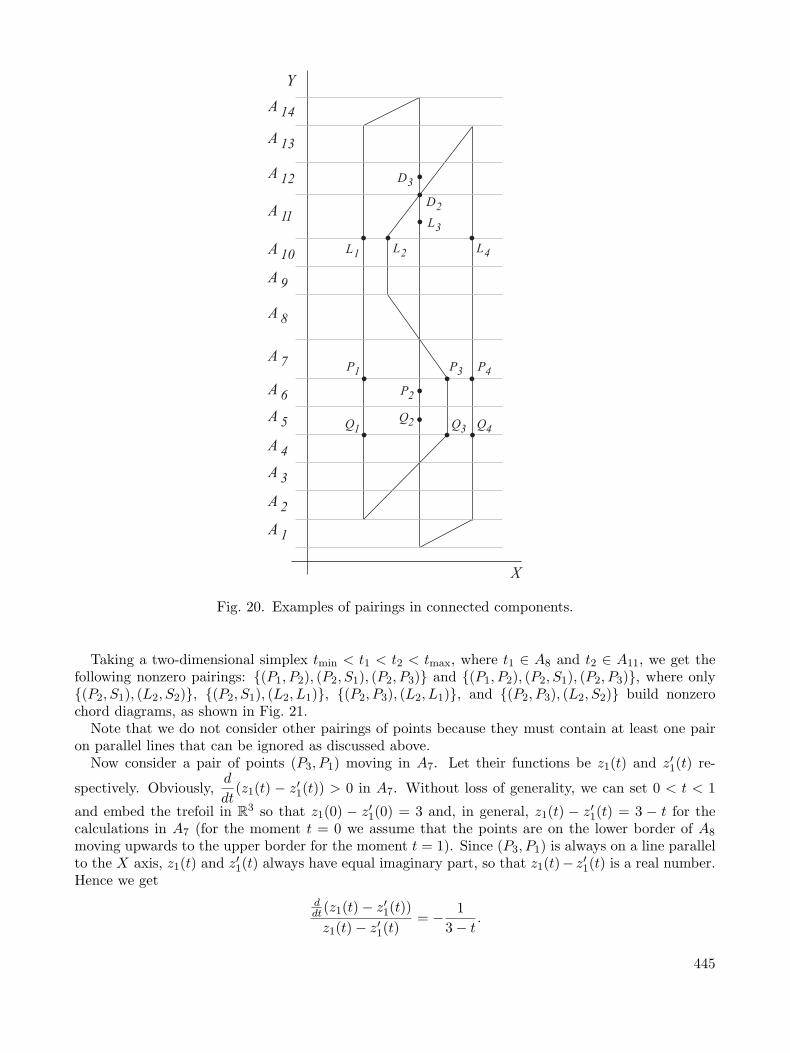
Fig. 20. Examples of pairings in connected components.

Taking a two-dimensional simplex tmin < t1 < t2 < tmax, where t1 ∈ A8 and t2 ∈ A11, we get thefollowing nonzero pairings: {(P1, P2), (P2, S1), (P2, P3)} and {(P1, P2), (P2, S1), (P2, P3)}, where only{(P2, S1), (L2, S2)}, {(P2, S1), (L2, L1)}, {(P2, P3), (L2, L1)}, and {(P2, P3), (L2, S2)} build nonzerochord diagrams, as shown in Fig. 21.

Note that we do not consider other pairings of points because they must contain at least one pairon parallel lines that can be ignored as discussed above.

Now consider a pair of points (P3, P1) moving in A7. Let their functions be z1(t) and z′1(t) re-

spectively. Obviously,d

dt(z1(t) − z′1(t)) > 0 in A7. Without loss of generality, we can set 0 < t < 1

and embed the trefoil in R3 so that z1(0) − z′1(0) = 3 and, in general, z1(t) − z′1(t) = 3 − t for the

calculations in A7 (for the moment t = 0 we assume that the points are on the lower border of A8

moving upwards to the upper border for the moment t = 1). Since (P3, P1) is always on a line parallelto the X axis, z1(t) and z′1(t) always have equal imaginary part, so that z1(t)− z′1(t) is a real number.Hence we get

ddt(z1(t)− z′1(t))z1(t)− z′1(t)

= − 1

3− t.

445

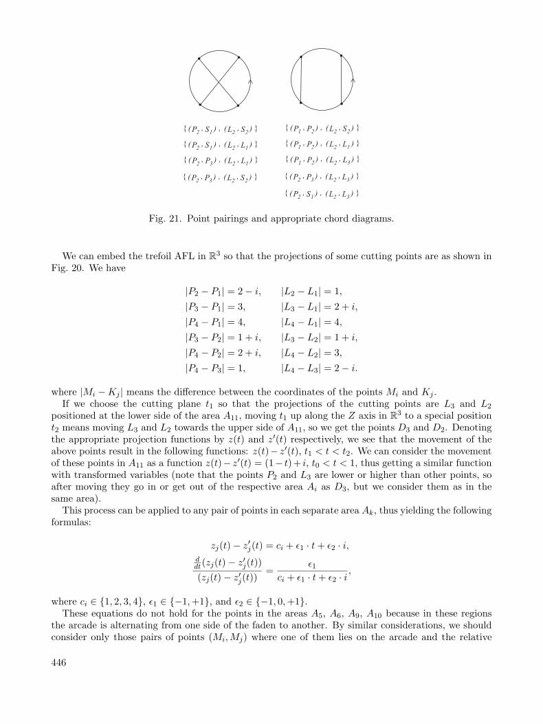
Fig. 21. Point pairings and appropriate chord diagrams.

We can embed the trefoil AFL in R3 so that the projections of some cutting points are as shown in

Fig. 20. We have

|P2 − P1| = 2− i, |L2 − L1| = 1,

|P3 − P1| = 3, |L3 − L1| = 2 + i,

|P4 − P1| = 4, |L4 − L1| = 4,

|P3 − P2| = 1 + i, |L3 − L2| = 1 + i,

|P4 − P2| = 2 + i, |L4 − L2| = 3,

|P4 − P3| = 1, |L4 − L3| = 2− i.

where |Mi −Kj | means the difference between the coordinates of the points Mi and Kj .If we choose the cutting plane t1 so that the projections of the cutting points are L3 and L2

positioned at the lower side of the area A11, moving t1 up along the Z axis in R3 to a special position

t2 means moving L3 and L2 towards the upper side of A11, so we get the points D3 and D2. Denotingthe appropriate projection functions by z(t) and z′(t) respectively, we see that the movement of theabove points result in the following functions: z(t)− z′(t), t1 < t < t2. We can consider the movementof these points in A11 as a function z(t)− z′(t) = (1− t)+ i, t0 < t < 1, thus getting a similar functionwith transformed variables (note that the points P2 and L3 are lower or higher than other points, soafter moving they go in or get out of the respective area Ai as D3, but we consider them as in thesame area).

This process can be applied to any pair of points in each separate area Ak, thus yielding the followingformulas:

zj(t)− z′j(t) = ci + ε1 · t+ ε2 · i,ddt(zj(t)− z′j(t))(zj(t)− z′j(t))

=ε1

ci + ε1 · t+ ε2 · i,

where ci ∈ {1, 2, 3, 4}, ε1 ∈ {−1,+1}, and ε2 ∈ {−1, 0,+1}.These equations do not hold for the points in the areas A5, A6, A9, A10 because in these regions

the arcade is alternating from one side of the faden to another. By similar considerations, we shouldconsider only those pairs of points (Mi,Mj) where one of them lies on the arcade and the relative

446

positions of such points can be calculated by the following formula:

zj(t)− z′j(t) = ε1 · i · (ε2 − t),

ddt(zj(t)− z′j(t))(zj(t)− z′j(t))

=−ε1 · i

ε1 · i · (ε2 − t),

where ε1 ∈ {−1,+1} and ε2 ∈ {0,+1}.Obviously, for the integral part in the Kontsevich formula the following equations hold:

∫

0<t1<···<tm<1

∑

(zi,z′i)∈P(−1)#P↓DP

m∧

j=1

d(zj − z′j)zj − z′j

=∑

Dl∈Dm

Dl

∑

Hk→Dl

(−1)#P↓∫

0<t1<···<tm<1

m∧

j=1

d(zj − z′j)zj − z′j

.

Hence, we get the following scheme for the computation of the Kontsevich integral:Input: AFL representation of a knot and an m-chord diagram Dl;

1. fix all the sets of points Hk = {(zi, z′i)} defining Dl;2. calculate as above

(−1)#P↓∫

0<t1<···<tm<1

m∧

j=1

d(zj − z′j)zj − z′j

and sum up the results.

The above integrals can be computed by standard methods.It is clear that the computational complexity of this method depends on the number of the point sets

Hk defining the given chord diagram. Using standard combinatorial methods one can easily computethe number of such sets that it is by far less than the number of summands in the standard formulaof the Kontsevich integral. On the other hand, the functions to be integrated are very simple, whichmakes the computation much easier.

5. Conclusions

In this article, we have shown how an old idea can be used to develop efficient algorithms to solveactual mathematical problems. In particular, we re-introduce the now forgotten AFL representationof knots introduced by Reidemeister some 80 years ago and develop efficient algorithms to find theholonomic representation of knots introduced by Vassiliev in the late 1990s and compute the rationalfactors of the Kontsevich integral for knots. It is the author’s hope that the methods described abovewill open new perspectives in the development of fast algorithms in this field.

REFERENCES

1. J. S. Birman and N. C. Wrinkle, “Holonomic and Legendrian parametrizations of knots,” J. KnotTheory Ramifications, 9, No. 3, 293–309 (2000).

2. S. Chmutov and S. Duzhin, “The Kontsevich integral,” Acta Appl. Math., 66, No. 2, 155–190(2001).

3. A. Gamkrelidze, “Algorithms in low-dimensional topology: holonomic parametrization of knots,”J. Math. Sci. (N.Y.) (to appear).

4. C. F. Gauss, “Zur mathematischen Theorie der electrodynamischen Wirkungen,” in: Werke,Koenigliche Gesellschaften der Wissenschaften zu Gottingen (1877), Vol. 5, p. 605.

5. M. Gusarov, “On n-equivalence of knots and invariants of finite degree,” Adv. Sov. Math., 18,173–192 (1994).

6. G. Hotz, “Ein Satz uber Mittellinien,” Arch. Math., 10, 314–320 (1959).

447

7. G. Hotz, “Arkadenfadendarstellung von Knoten und eine neue Darstellung der Knotengruppe,”Abh. Math. Sem. Univ. Hamburg, 24, 132–148 (1960).

8. G. Hotz, “An efficient algorithm to decide the knot problem,“ Bull. Georgian Natl. Acad. Sci.(N.S.), 2, No. 3, 5–17 (2008).

9. M. Kontsevich, “Vassiliev’s knot invariants,” in: Adv. Sov. Math., 16, Part 2, 137–150 (1993).10. K. Reidemeister, Knotentheorie, Springer, Berlin (1932).11. V. A. Vassiliev, “Cohomology of knot spaces,” Adv. Sov. Math., 1, 23–69 (1990).12. V. A. Vassiliev, Complements of Discriminants of Smooth Maps: Topology and Applications,

Trans. Math. Monogr., 98, Am. Math. Soc., Providence, Rhode Island (1992).13. V. A. Vassiliev, “Holonomic links and Smale principles for multisingularities,” J. Knot Theory

Ramifications, 6, No. 1, 115–123 (1997).

A. GamkrelidzeDepartment of Computer Science,I. Javakhishvili Tbilisi State University, Tbilisi, GeorgiaE-mail: alexander.gamkrelidze@tsu.ge

448