Embed Size (px)
Citation preview
© LCPC - 2011
ALIZE-LCPC Software
version 1.3
User manual
January 2011
Official distributor: itech 12-16 rue de Vincennes 93100 Montreuil - FRANCE Tel.: +33 1 48 70 47 41 - Fax: +33 1 48 59 12 24 – E-mail: [email protected]
www.itech-soft.com

Contents
ALIZE-LCPC Routes - User manual version 1.3 page 1
Contents
1. Introduction to the user's manual 3
1.1 - Objectives and general use of Alize-LCPC Routes 3 1.2 - Reference documents 4 1.3 - General architecture 4 1.4 - Required computing configuration, protection against hacking 5
2. Installation of the Alize-LCPC Routes software 7
2.1 - Automatic installation using the Autorun procedure 7 2.2 - Manual installation 7 2.3 - Comments 7
3. Launching the program 9
3.1 - Application startup 9 3.2 - Alize-LCPC configuration 9 3.3 - The files generated by the software 11 3.4 - To move from one data window to another 11 3.5 - Important remark: Clickable boxes to access pull-down menus 11
4. Data preparation: The pavement structure 13
4.1 - Principle of pavement structure modeling 13 4.2 - Creating and modifying the Structure data 13 4.3 – Some complementary information about data input steps 15 4.4 - Consulting and importation of the Catalogue 1998 forms 17 4.5 - Data file recording and re-loading 17
5. Data preparation: The applied loads 19
5.1 - Definition of the reference load 19 5.2 - Definition of special loads 20 5.3 - Special pseudo-rectangular loads 22 5.4 - Navigating between the Structure window and Special load window 22
6. Performing computation 25
6.1 - The two computation modes 25 6.2 - Commands for launching computation 25 6.3 - Execution of computation in the Grid-seca mode 27
Contents
ALIZE-LCPC Routes - User manual version 1.3 page 2
7. Results of mechanical computation 31
7.1 - Results from standard computation 31 7.2 - Results from Grid-seca computations 33 7.3 - Results of Grid-seca computation: transversal damage profiles 37
8. Computation of allowable values 41
8.1 - Allowable value window 41 8.2 - Information about the material mechanical library 42
9. Alize-Frost thaw: Data preparation 45
9.1 - Description of the problem 45 9.2 - A few additional recommendation for data input 48 9.3 - Saving and reading of data files 50 9.4 - Definition of initial and boundary conditions 50 9.5 - Calculation of the frost quantity Qpf allowable by the pavement foundation 52 9.6 - Precision about the Alize-Gel material library 54
10. Alize-Frost thaw: Launching computation and editing results 55
10.1 - Commands for launching the computation 55 10.2 - Results of the Alize-Frost thaw computation 56
11. Alize Back-calculation: Data, computation and results 63
11.1 - The problem concerned by the Alize Back-calculation module 63 11.2 - Preparing the data for back-calculation 64 11.3 - Launching Alize-Back calculation 69 11.4 - Alize-Back calculation: results 69
12. Appendix A1: The rational pavement design approach 73
A1.1 - General framework of rational pavement design 73 A2.2 - General approach to rational pavement design 73 A3.3 - The mechanical computation model 77
13. Annexe A2 : Principles of the Frost-thaw verification 79
A2.2 - Frost–thaw behavior of soils 79 A2.3 - Place of the frost-thaw verification in the pavement design 80 A2.4 - Definitions and notations 81 A2.5 - General organization of the frost-thaw verification 81

1- Introduction to the user's manual
ALIZE-LCPC Routes - User manual version 1.3 page 3
1
1. Introduction to the user's manual
1.1 - Objectives and general use of Alize-LCPC Routes
The Alize-LCPC Routes User's Manual guides the user for employing this software application. It presents the different possibilities and functionalities of the program as well as the set of installation conditions. In this manual, the "Alize-LCPC Routes" software will be also designated by both the terms "Alize-LCPC" and "Alize". It is assumed that the user has been adequately trained in running the Microsoft Windows operating system and is capable of mastering the various associated interfaces and peripherals. Alize-LCPC Routes has been set up to implement the rational mechanical design method for pavement structures, as developed by the LCPC and SETRA French organizations; this method constitutes the regulatory approach for designing pavements throughout the French national road network and moreover has been adopted by many other road project development agencies. The basis of the rational design technique is presented in Appendix A1 for what concerns the pavement mechanical design, and Appendix A2 for pavement frost-thaw verification, which is also considered by the program. The integral version of Alize-LCPC includes three main modules:
The mechanical computation module based on the determination of the stresses and strains created in the road materials by the traffic loads, named “Alize-mechanical module”.
The module dedicated to the verification of the design as regard the pavement frost-thaw behavior, named “Alize-frost thaw module”
The back-calculation module used for the computation of the elastic modules of the pavement materials from the measured deflection bowls, named the “Alize-back calculation module”.
Alize-LCPC may be distributed in the complete integral version including the three modules Alize-mechanical, Alize-frost thaw and Alize-back calculation, or in one of the three following limited versions: Alize-mechanical alone, or Alize-frost thaw alone, or Alize-mechanical + Alize-back calculation. This User’s manual concerns both the integral version and the three partial versions of the software:
The users of the integral version are concerned by the whole manual (11 parts) and the two appendixes A1 and A2.
The users of the limited version Alize-mechanical are concerned by the parts 1 to 8 and Appendix A1,
The users of the limited version Alize-frost thaw are concerned by the parts 1 to 3, 9 to 10 and Appendix A2,
The users of the limited version Alize-mechanical + back calculation are concerned by the parts 1 to 8 and 11, and Appendix A1.

1- Introduction to the user's manual
ALIZE-LCPC Routes - User manual version 1.3 page 4
1.2 - Reference documents
The following reference documents provide a more detailed presentation of the French design method :
The French Design guide for pavement structures, LCPC-SETRA 1994 which present in greater detail the principles of the rational pavement design
The Catalogue of new standard pavement structures, LCPC-SETRA 1998
The Technical Guide of Variant Specifications, SETRA 2003.
These two later documents describe the application conditions of rational design to the pavement structures of the French national road network, accordingly to the French official specifications.
The computation algorithm of the Alize-frost thaw module is derived from the Gel1d software, a MS-Dos application developed by LCPC, not yet distributed since 2002. For more details about the Gel1d software, refer to «Gel1d, Modélisation de la congélation des structures de chaussées multicouches», LCPC 1999. In addition to this computation algorithm, the Alize-frost thaw module is built around a new graphical user interface (GUI) including help facilities, which are not comprised in the original Gel1d Dos program.
1.3 - General architecture
The general architecture of the Alize-LCPC program aims to facilitate, to the greatest extent possible, implementation of the rational pavement design method. This objective leads to following functionalities: Alize-mechanical module :
Definition of the pavement structure: thickness, elasticity parameters of the different layers and interface condition between layers;
Definition of the loading applied at the surface (reference load or other loading, named “special loading”);
Determination of the stresses and/or strains allowable by the different materials, according to their damage law parameters and the traffic condition;
Computation of the stresses and strains created in the pavement materials by the traffic loads;
Graphical display of the mechanical computation results;
Assistance and support for the practical choice of both hypotheses and numerical values of the various parameters need by the mechanical computation, in accordance with the specifications of the Technical Guide LCPC-SETRA and/or the New Structures Catalogue;
Management of a library (the mechanicam library) including both standard materials which mechanical properties are defined by the LCPC-SETRA documents referred above, and customized materials defined by the user.
1- Introduction to the user's manual
ALIZE-LCPC Routes - User manual version 1.3 page 5
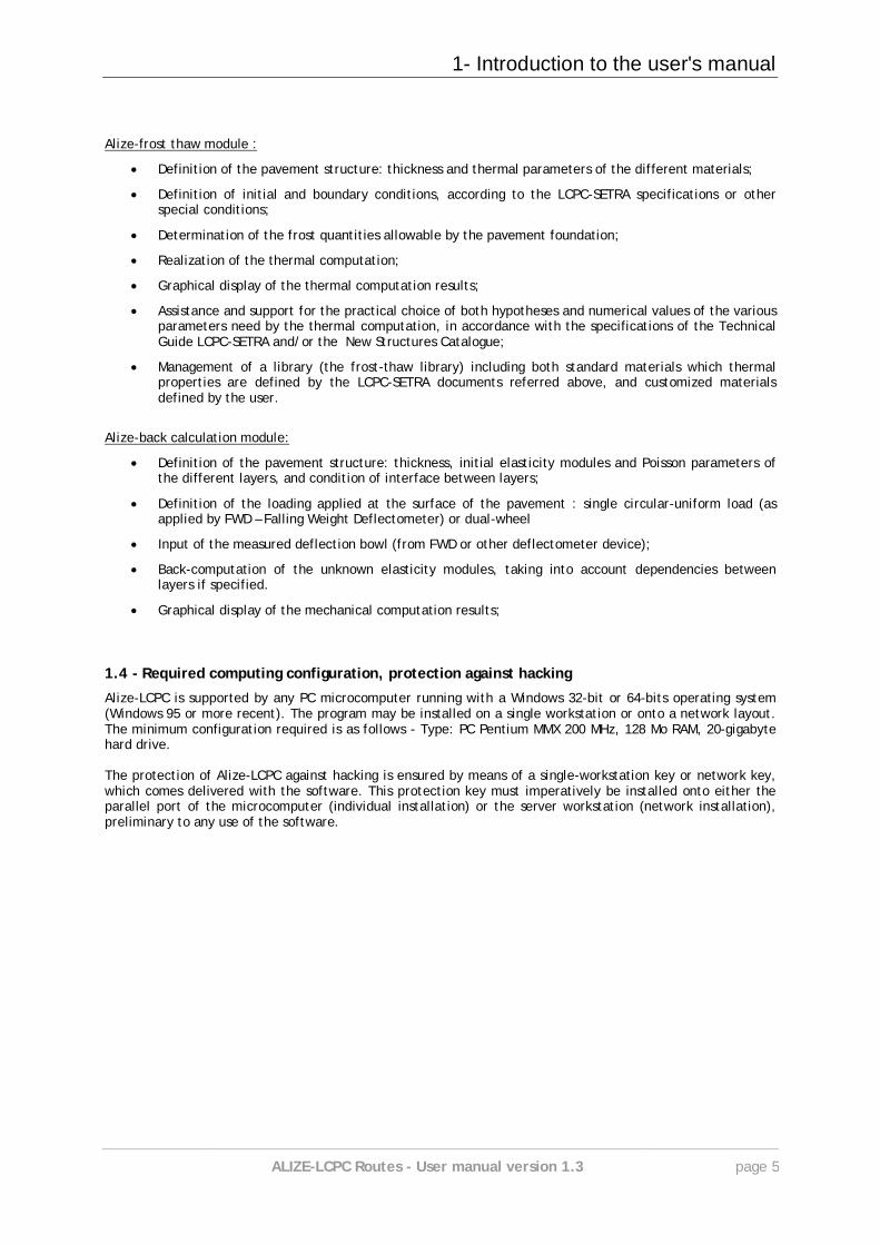
Alize-frost thaw module :
Definition of the pavement structure: thickness and thermal parameters of the different materials;
Definition of initial and boundary conditions, according to the LCPC-SETRA specifications or other special conditions;
Determination of the frost quantities allowable by the pavement foundation;
Realization of the thermal computation;
Graphical display of the thermal computation results;
Assistance and support for the practical choice of both hypotheses and numerical values of the various parameters need by the thermal computation, in accordance with the specifications of the Technical Guide LCPC-SETRA and/or the New Structures Catalogue;
Management of a library (the frost-thaw library) including both standard materials which thermal properties are defined by the LCPC-SETRA documents referred above, and customized materials defined by the user.
Alize-back calculation module:
Definition of the pavement structure: thickness, initial elasticity modules and Poisson parameters of the different layers, and condition of interface between layers;
Definition of the loading applied at the surface of the pavement : single circular-uniform load (as applied by FWD – Falling Weight Deflectometer) or dual-wheel
Input of the measured deflection bowl (from FWD or other deflectometer device);
Back-computation of the unknown elasticity modules, taking into account dependencies between layers if specified.
Graphical display of the mechanical computation results;
1.4 - Required computing configuration, protection against hacking
Alize-LCPC is supported by any PC microcomputer running with a Windows 32-bit or 64-bits operating system (Windows 95 or more recent). The program may be installed on a single workstation or onto a network layout. The minimum configuration required is as follows - Type: PC Pentium MMX 200 MHz, 128 Mo RAM, 20-gigabyte hard drive. The protection of Alize-LCPC against hacking is ensured by means of a single-workstation key or network key, which comes delivered with the software. This protection key must imperatively be installed onto either the parallel port of the microcomputer (individual installation) or the server workstation (network installation), preliminary to any use of the software.

2- Installation of the Alizé-LCPC Routes software
ALIZE-LCPC Routes - User manual version 1.3 page 7
2
2. Installation of the Alize-LCPC Routes software
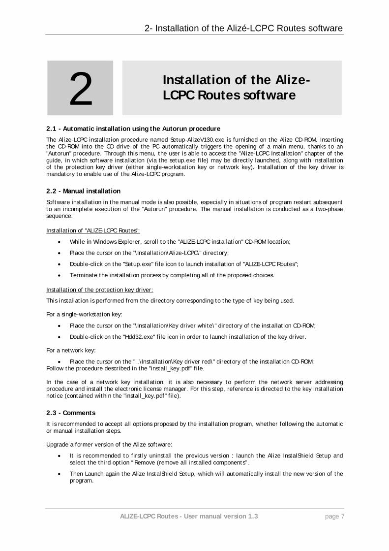
2.1 - Automatic installation using the Autorun procedure
The Alize-LCPC installation procedure named Setup-AlizeV130.exe is furnished on the Alize CD-ROM. Inserting the CD-ROM into the CD drive of the PC automatically triggers the opening of a main menu, thanks to an "Autorun" procedure. Through this menu, the user is able to access the "Alize-LCPC Installation" chapter of the guide, in which software installation (via the setup.exe file) may be directly launched, along with installation of the protection key driver (either single-workstation key or network key). Installation of the key driver is mandatory to enable use of the Alize-LCPC program.
2.2 - Manual installation
Software installation in the manual mode is also possible, especially in situations of program restart subsequent to an incomplete execution of the "Autorun" procedure. The manual installation is conducted as a two-phase sequence:
Installation of "ALIZE-LCPC Routes":
While in Windows Explorer, scroll to the "ALIZE-LCPC installation" CD-ROM location;
Place the cursor on the "\Installation\Alize-LCPC\" directory;
Double-click on the "Setup.exe" file icon to launch installation of "ALIZE-LCPC Routes";
Terminate the installation process by completing all of the proposed choices.
Installation of the protection key driver:
This installation is performed from the directory corresponding to the type of key being used. For a single-workstation key:
Place the cursor on the "\Installation\Key driver white\" directory of the installation CD-ROM;
Double-click on the "Hdd32.exe" file icon in order to launch installation of the key driver. For a network key:
Place the cursor on the "..\Installation\Key driver red\" directory of the installation CD-ROM; Follow the procedure described in the "install_key.pdf" file. In the case of a network key installation, it is also necessary to perform the network server addressing procedure and install the electronic license manager. For this step, reference is directed to the key installation notice (contained within the "install_key.pdf" file).
2.3 - Comments
It is recommended to accept all options proposed by the installation program, whether following the automatic or manual installation steps. Upgrade a former version of the Alize software:
It is recommended to firstly uninstall the previous version : launch the Alize InstalShield Setup and select the third option “Remove (remove all installed components”.
Then Launch again the Alize InstalShield Setup, which will automatically install the new version of the program.

3- Launching the program
ALIZE-LCPC Routes - User manual version 1.3 page 9
3
3. Launching the program
3.1 - Application startup
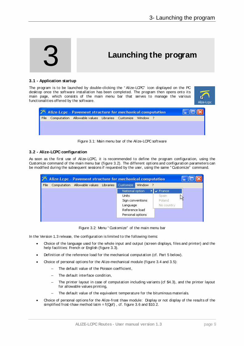
The program is to be launched by double-clicking the “Alize-LCPC” icon displayed on the PC desktop once the software installation has been completed. The program then opens onto its main page, which consists of the main menu bar that serves to manage the various functionalities offered by the software.
Figure 3.1: Main menu bar of the Alize-LCPC software
3.2 - Alize-LCPC configuration
As soon as the first use of Alize-LCPC, it is recommended to define the program configuration, using the Customize command of the main menu bar (figure 3.2). The different options and configuration parameters can be modified during the subsequent sessions if requested by the user, using the same ”Customize” command.
Figure 3.2: Menu “Customize” of the main menu bar In the Version 1.3 release, the configuration is limited to the following items:
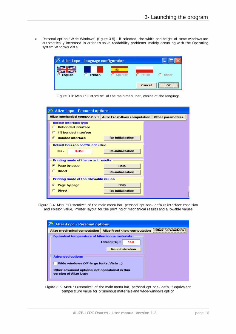
Choice of the language used for the whole input and output (screen displays, files and printer) and the help facilities: French or English (figure 3.3).
Definition of the reference load for the mechanical computation (cf. Part 5 below).
Choice of personal options for the Alize-mechanical module (figure 3.4 and 3.5):
– The default value of the Poisson coefficient,
– The default interface condition,
– The printer layout in case of computation including variants (cf $4.3), and the printer layout for allowable values printing,
– The default value of the equivalent temperature for the bituminous materials.
Choice of personal options for the Alize-frost thaw module: Display or not display of the results of the simplified frost-thaw method Iatm = f(Qpf) , cf. figure 3.6 and $10.2.
3- Launching the program
ALIZE-LCPC Routes - User manual version 1.3 page 10
Personal option “Wide Windows” (figure 3.5) : if selected, the width and height of some windows are automatically increased in order to solve readability problems, mainly occurring with the Operating system Windows Vista.
Figure 3.3: Menu “Customize” of the main menu bar, choice of the language
Figure 3.4: Menu “Customize” of the main menu bar, personal options - default interface condition and Poisson value, Printer layout for the printing of mechanical results and allowable values
Figure 3.5: Menu “Customize” of the main menu bar, personal options - default equivalent temperature value for bituminous materials and Wide-windows option
3- Launching the program
ALIZE-LCPC Routes - User manual version 1.3 page 11
Figure 3.6: Menu “Customize” of the main menu bar, personal options – Display or not display the results of the simplified frost-thaw method Iatm = f(Qpf) (Alize-frost thaw module)
The other imposed configuration options are given below:
units: meter (m), mega-Newton (MN) and all associated units. It should be noted that both the Young's modulus and pressure values are thus expressed in MPa. In addition, the Frost-thaw module uses the following units: kilogram (Kg), Watt (W), Celsius degree (°C) and associated units.
sign conventions: – all expansion and tension stresses and strains are counted as negative values (mechanical
computation results), – deflection considered as a positive value (in the direction of gravity), – allowable values expressed as positive numbers;
3.3 - The files generated by the software In common use, data need for computation are saved in data files by mean of the command Files of the main menu bar. The command File manages the following data files :
Pavement structure data files for mechanical computation : extension .dat, cf. Part 4 below; Special load data files for mechanical computation : extension .chg, cf. Part 5 below; Pavement structure data files for frost-thaw computation : extension .dag, cf. Part 4 below; Pavement structure-Loading-Deflection bowl files for backcalculation : extension .mwd, cf. Part 11
below.
The results of the computation can be saved – if requested –in output Ascii files as follows : Allowable values computation files : extension .adm, cf. Part 8 below of the present manual; Results of mechanical computation : extension .res, cf. Part 7 below; Results of frost-thaw computation : extension .res, cf. §10.2 below; Results of backcalculation : extension -retro.res, cf. Part11 beloow.
3.4 - To move from one data window to another Two, three or the four data windows (Pavement structure data, Special loading data, Frost-thaw data and Backcalculation data) can be simultaneously loaded. But only one of them may be active, and the other are not loaded but not visible. In order to move from one dat window to another, use the command Window of the main menu bar.
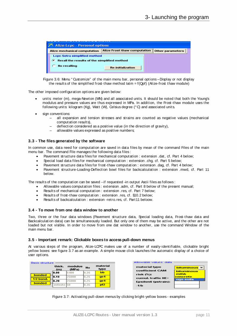
3.5 - Important remark: Clickable boxes to access pull-down menus
At various steps of the program, Alize-LCPC makes use of a number of easily-identifiable, clickable bright yellow boxes: see figure 3.7 as an example. A simple mouse click launches the automatic display of a choice of user options.
Figure 3.7: Activating pull-down menus by clicking bright-yellow boxes - examples

4- Data preparation: The pavement structure
ALIZE-LCPC Routes - User manual version 1.3 page 13
4
4. Data preparation: The pavement structure
4.1 - Principle of pavement structure modeling
Pavement modeling, according to the rational design approach, relies upon a representation of the structure by means of a multilayer structure having an isotropic linear elastic behavior. The various layers of material constituting the structure have constant thickness; moreover, their expansion within the horizontal plane XoY is infinite. Expansion along the vertical direction ZZ of the lower layer of the multilayer foundation, which generally represents the substratum or supporting soil, is also assumed infinite. The following set of parameters are needed for each layer :
thickness H;
Young's modulus E of the material;
Poisson's ratio of the material (denoted "Nu" in Alize-LCPC); and
interface conditions at the layer's upper and lower extremes, with the adjoining layers. Three types of interface are available in order to characterize how the interface functions between adjacent layers: bonded, sliding, or semi-bonded. The semi-bonded interface condition is specified by the Technical guide French pavement design LCPC-SETRA, for modeling the contact between some materials. In case of semi-bonded interface, two successive computations are automatically performed, the first one considering bonded interface and the second one considering sliding interface. The semi-bonded condition is then considered as the mean value of the stresses and strains resulting from these two computations.
4.2 - Creating and modifying the Structure data
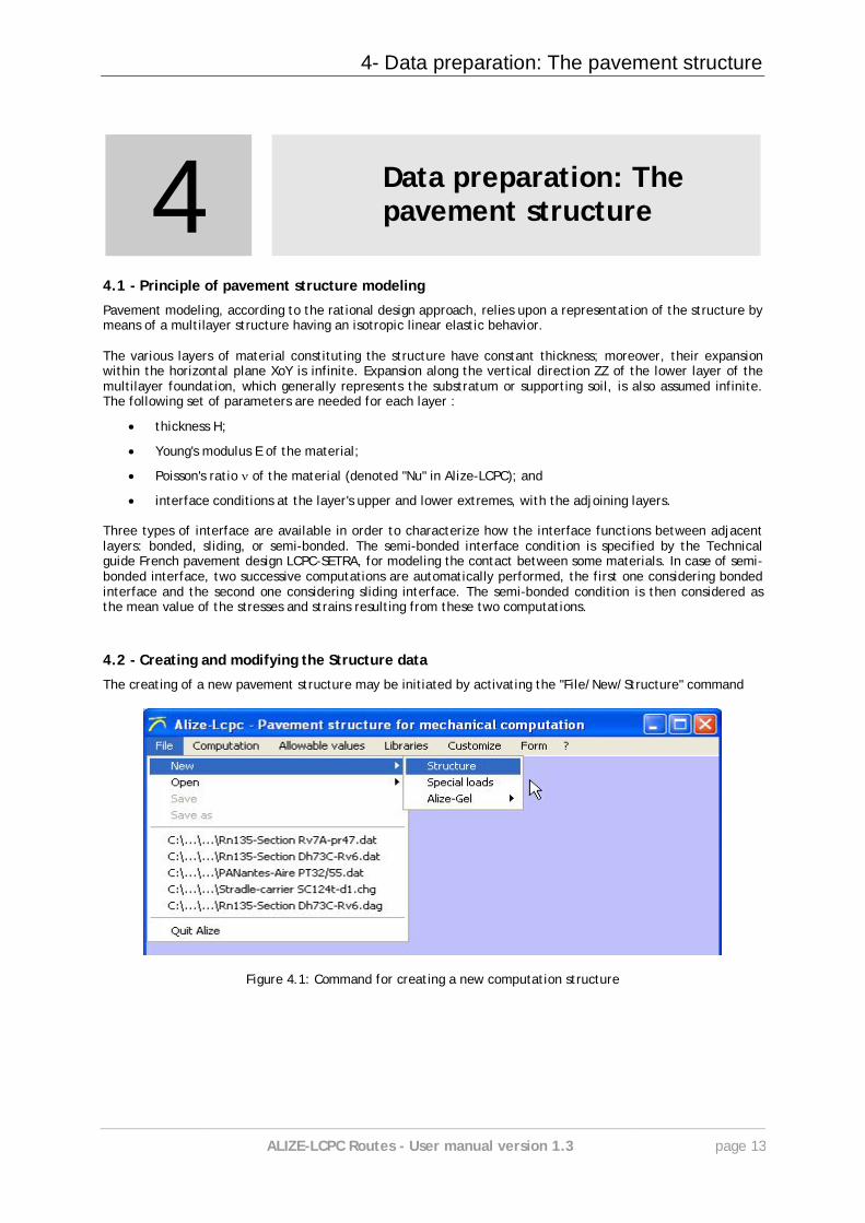
The creating of a new pavement structure may be initiated by activating the "File/New/Structure" command
Figure 4.1: Command for creating a new computation structure
4- Data preparation: The pavement structure
ALIZE-LCPC Routes - User manual version 1.3 page 14
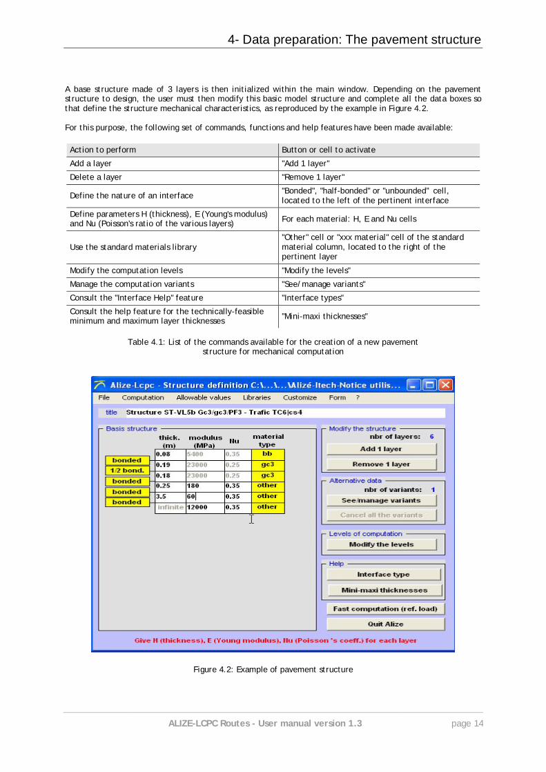
A base structure made of 3 layers is then initialized within the main window. Depending on the pavement structure to design, the user must then modify this basic model structure and complete all the data boxes so that define the structure mechanical characteristics, as reproduced by the example in Figure 4.2. For this purpose, the following set of commands, functions and help features have been made available: Action to perform Button or cell to activate
Add a layer "Add 1 layer"
Delete a layer "Remove 1 layer"
Define the nature of an interface "Bonded", "half-bonded" or "unbounded” cell, located to the left of the pertinent interface
Define parameters H (thickness), E (Young's modulus) and Nu (Poisson's ratio of the various layers) For each material: H, E and Nu cells
Use the standard materials library "Other" cell or "xxx material" cell of the standard material column, located to the right of the pertinent layer
Modify the computation levels "Modify the levels"
Manage the computation variants "See/manage variants"
Consult the "Interface Help" feature "Interface types"
Consult the help feature for the technically-feasible minimum and maximum layer thicknesses "Mini-maxi thicknesses"
Table 4.1: List of the commands available for the creation of a new pavement
structure for mechanical computation
Figure 4.2: Example of pavement structure
4- Data preparation: The pavement structure
ALIZE-LCPC Routes - User manual version 1.3 page 15
4.3 – Some complementary information about data input steps In pursuing these various steps, the user is guided by a very detailed set of help messages and warning messages in the event of anomaly or error. A few of complementary information are provided below:
The decimal separator used for entering numerical values must be that for which the Windows operating system has been configured on the host PC (see Settings/Regional and Language Options/Decimal Symbol).
It is strongly advised to fill the structure title boxe in order to facilitate its subsequent identification, e.g. during future use of the data or printout of computation results.
The maximum number of layers of materials constituting the pavement structure is limited to 15, with a minimum of 1.
The default interface condition may be defined using the “Customize” command of the main menu bar, which open the window “Alize-Lcpc – Personal options” (see Part 3 above and figure 4.4). The default value of the Poisson coefficient, and the default value of equivalent temperature of bituminous materials, may also be modified using the same command.
The computation of internal stresses and strains within the materials is performed at two levels in each material layer. These levels implicitly consist of the interfaces between layers, i.e. those levels at which maximum internal stresses are generally obtained. The "Computation levels" command enables modifying this implicit choice.
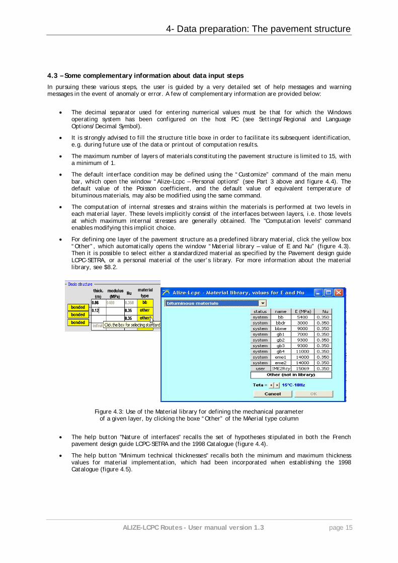
For defining one layer of the pavement structure as a predefined library material, click the yellow box “Other”, which automatically opens the window “Material library – value of E and Nu” (figure 4.3). Then it is possible to select either a standardized material as specified by the Pavement design guide LCPC-SETRA, or a personal material of the user’s library. For more information about the material library, see $8.2.
Figure 4.3: Use of the Material library for defining the mechanical parameter
of a given layer, by clicking the boxe “Other” of the MAerial type column
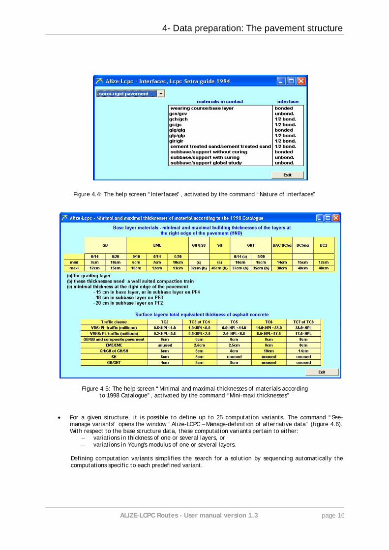
The help button "Nature of interfaces" recalls the set of hypotheses stipulated in both the French pavement design guide LCPC-SETRA and the 1998 Catalogue (figure 4.4).
The help button "Minimum technical thicknesses" recalls both the minimum and maximum thickness values for material implementation, which had been incorporated when establishing the 1998 Catalogue (figure 4.5).
4- Data preparation: The pavement structure
ALIZE-LCPC Routes - User manual version 1.3 page 16
Figure 4.4: The help screen “Interfaces”, activated by the command “Nature of interfaces”
Figure 4.5: The help screen “Minimal and maximal thicknesses of materials according to 1998 Catalogue”, activated by the command “Mini-maxi thicknesses”
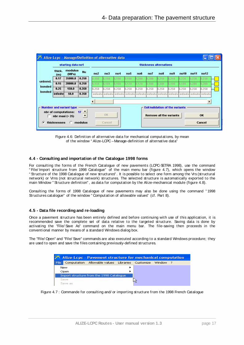
For a given structure, it is possible to define up to 25 computation variants. The command “See-manage variants” opens the window “Alize-LCPC – Manage-definition of alternative data” (figure 4.6). With respect to the base structure data, these computation variants pertain to either:
– variations in thickness of one or several layers, or – variations in Young's modulus of one or several layers.
Defining computation variants simplifies the search for a solution by sequencing automatically the computations specific to each predefined variant.
4- Data preparation: The pavement structure
ALIZE-LCPC Routes - User manual version 1.3 page 17
Figure 4.6: Definition of alternative data for mechanical computations, by mean of the window “Alize-LCPC – Manage-definition of alternative data”
4.4 - Consulting and importation of the Catalogue 1998 forms
For consulting the forms of the French Catalogue of new pavements (LCPC-SETRA 1998), use the command “File/Import structure from 1998 Catalogue” of the main menu bar (figure 4.7), which opens the window “Structure of the 1998 Catalogue of new structures”. It is possible to select one form among the Vrs (structural network) or Vrns (not structural network) structures. The selected structure is automatically exported to the main Window ”Structure definition”, as data for computation by the Alize-mechanical module (figure 4.8). Consulting the forms of 1998 Catalogue of new pavements may also be done using the command ”1998 Structures catalogue” of the window ”Computation of allowable values” (cf. Part 8).
4.5 - Data file recording and re-loading
Once a pavement structure has been entirely defined and before continuing with use of this application, it is recommended save the complete set of data relative to the targeted structure. Saving data is done by activating the "File/Save As" command on the main menu bar. The file-saving then proceeds in the conventional manner by means of a standard Windows dialog box. The "File/Open" and "File/Save" commands are also executed according to a standard Windows procedure; they are used to open and save the files containing previously-defined structures.
Figure 4.7 : Commande for consulting and/or importing structure from the 1998 French Catalogue

4- Data preparation: The pavement structure
ALIZE-LCPC Routes - User manual version 1.3 page 18
Figure 4.9 : Window Structures of the 1998 Cataologue LCPC-SETRA 1998
5- Data preparation: The appied loads
ALIZE-LCPC Routes - User manual version 1.3 page 19
5
5. Data preparation: The applied loads
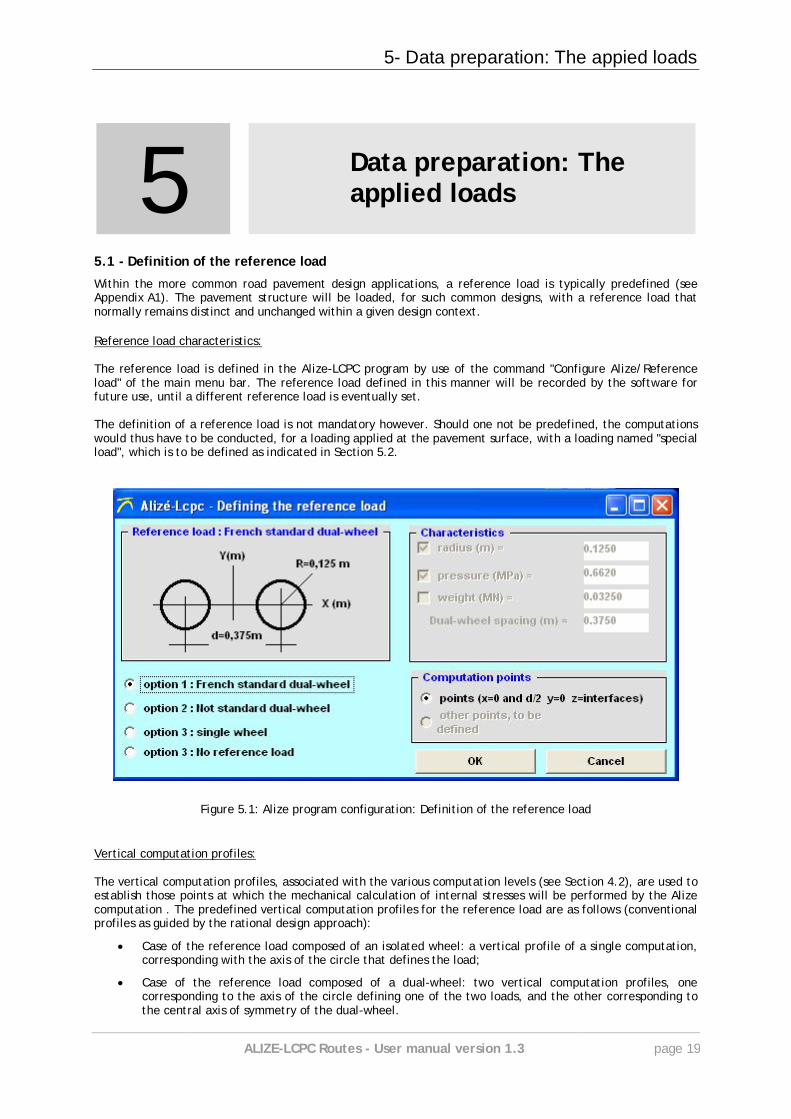
5.1 - Definition of the reference load Within the more common road pavement design applications, a reference load is typically predefined (see Appendix A1). The pavement structure will be loaded, for such common designs, with a reference load that normally remains distinct and unchanged within a given design context. Reference load characteristics: The reference load is defined in the Alize-LCPC program by use of the command "Configure Alize/Reference load" of the main menu bar. The reference load defined in this manner will be recorded by the software for future use, until a different reference load is eventually set. The definition of a reference load is not mandatory however. Should one not be predefined, the computations would thus have to be conducted, for a loading applied at the pavement surface, with a loading named "special load", which is to be defined as indicated in Section 5.2.
Figure 5.1: Alize program configuration: Definition of the reference load Vertical computation profiles: The vertical computation profiles, associated with the various computation levels (see Section 4.2), are used to establish those points at which the mechanical calculation of internal stresses will be performed by the Alize computation . The predefined vertical computation profiles for the reference load are as follows (conventional profiles as guided by the rational design approach):
Case of the reference load composed of an isolated wheel: a vertical profile of a single computation, corresponding with the axis of the circle that defines the load;
Case of the reference load composed of a dual-wheel: two vertical computation profiles, one corresponding to the axis of the circle defining one of the two loads, and the other corresponding to the central axis of symmetry of the dual-wheel.

5- Data preparation: The appied loads
ALIZE-LCPC Routes - User manual version 1.3 page 20
The computation profiles connected with the reference load cannot not be modified. If such a modification is requested, use the Special load definition procedure as described in Section 5.2.
5.2 - Definition of special loads
Characteristics of special loadings:
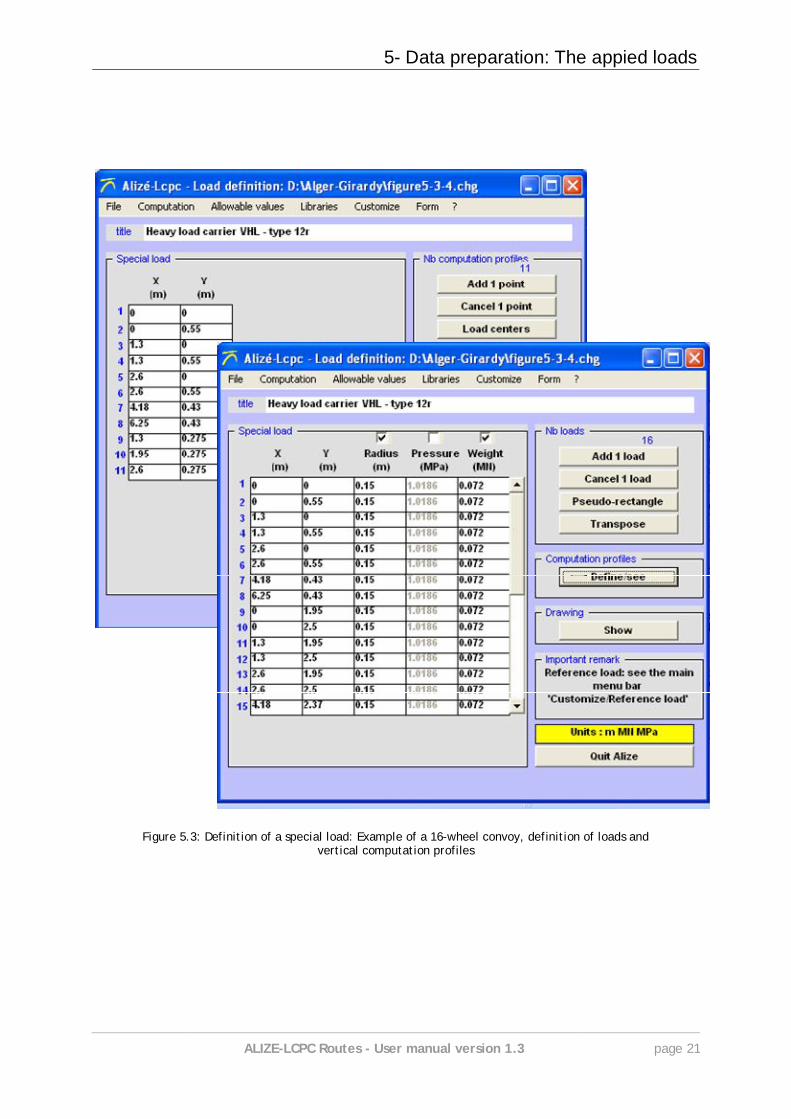
A special load is composed of a set of unit vertical circular loads, applied to the pavement surface. The number of isolated loads constituting this complete loading may vary between 1 and 1,000. The load characteristics (radius, weight and pressure) are capable of varying from one isolated load to the next.
Vertical computation profiles:
In addition to the data that serve to define the entire special loading in terms of both geometry and loads applied to the various wheels, it is also often necessary to determine the vertical computation profiles. Such however is not the case when the computations are subsequently executed in the "Grid-seca computation" mode (see Section 6.3).
Figure 5.2: Command for the creation of a new special load The input of these two data sets (loading characteristics and vertical computation profiles) is activated by the "File/New/Special loads" command of the main menu bar.
Saving to a file
Once a special loading has been completely defined and before continuing with use of this application, it is recommended to save the entire set of data relative to the special loading, by means of the "File/Save as" command on the main menu bar (see Section 4.1). The general comments expressed in Section 4.1, with respect to both saving and opening data files via the standard Windows dialog boxes, are also applicable herein.
5- Data preparation: The appied loads
ALIZE-LCPC Routes - User manual version 1.3 page 21
Figure 5.3: Definition of a special load: Example of a 16-wheel convoy, definition of loads and vertical computation profiles
5- Data preparation: The appied loads
ALIZE-LCPC Routes - User manual version 1.3 page 22
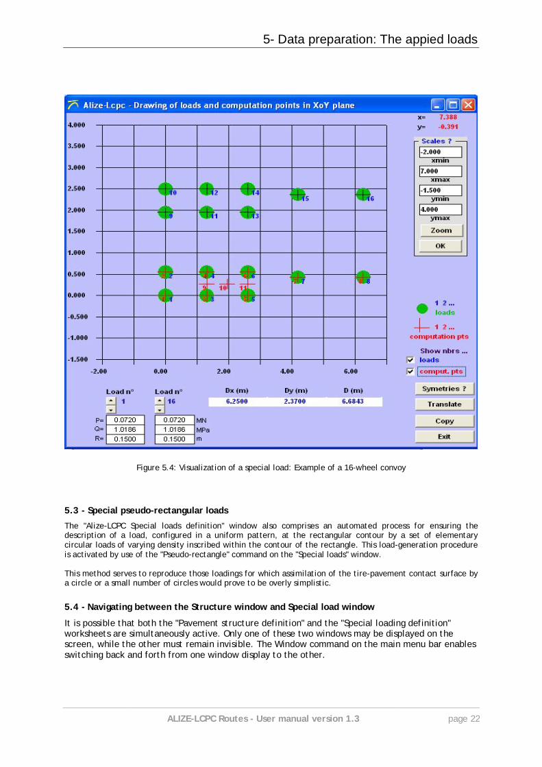
Figure 5.4: Visualization of a special load: Example of a 16-wheel convoy
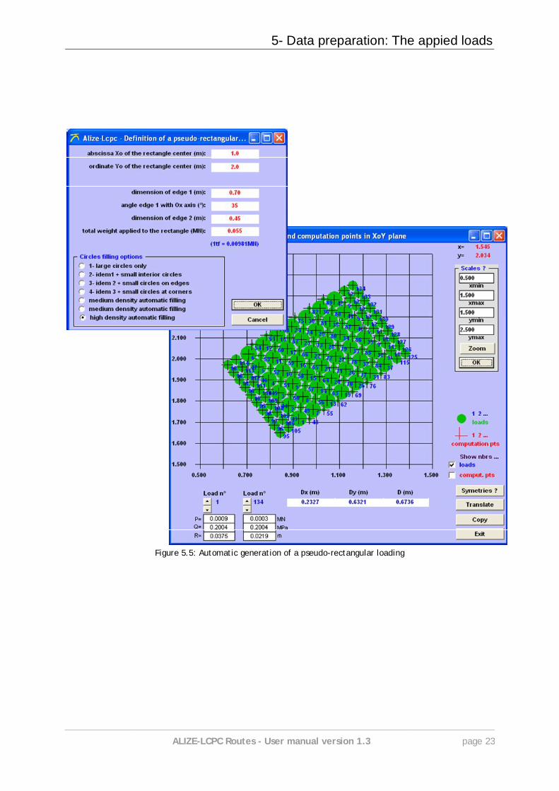
5.3 - Special pseudo-rectangular loads
The "Alize-LCPC Special loads definition" window also comprises an automated process for ensuring the description of a load, configured in a uniform pattern, at the rectangular contour by a set of elementary circular loads of varying density inscribed within the contour of the rectangle. This load-generation procedure is activated by use of the "Pseudo-rectangle" command on the "Special loads" window. This method serves to reproduce those loadings for which assimilation of the tire-pavement contact surface by a circle or a small number of circles would prove to be overly simplistic.
5.4 - Navigating between the Structure window and Special load window
It is possible that both the "Pavement structure definition" and the "Special loading definition" worksheets are simultaneously active. Only one of these two windows may be displayed on the screen, while the other must remain invisible. The Window command on the main menu bar enables switching back and forth from one window display to the other.
5- Data preparation: The appied loads
ALIZE-LCPC Routes - User manual version 1.3 page 23
Figure 5.5: Automatic generation of a pseudo-rectangular loading

6- Performing computation
ALIZE-LCPC Routes - User manual version 1.3 page 25
6
6. Performing computation
6.1 - The two computation modes
Prior to initiating the mechanical computation, the user must specify both the pavement structure and the loading (reference load or special loading), for which the computation has to be performed. These two data sets are managed by the application in an independent manner:
saving on two distinct, independent and specific files;
display on two separate and unlinked screen windows;
possibility of performing computations for any structure-loading association. Two computation modes are indeed possible:
the standard type of computation, for which results will be calculated at points (called "computation points") located on the vertical computation profiles defined along with the loading (see Sections 5.1 and 5.2). On each vertical profile, the computations will be carried out at 2 points of each layer (see Section 4.2, Computation levels). This computation mode is normally selected for more common design needs. Results will be presented in the form of tables of stress values calculated at each of the computation points.
the "grid-seca" type of computation, for which the vertical computation profiles are defined by a grid. This set of computation points is then used to generate, at each computation level, a cluster of square mesh points, whose interval and range are set by the user. The results will be presented in the form of either longitudinal and transversal profiles, or 2D or 3D isovalue surfaces. This second mode for presenting computations enables a more complete visualization of the overall operations of the pavement structure for a given loading. It is also useful in applications that study the behavior of pavements submitted to complex loadings. Under such conditions, the pre-evaluation of maximum stress localization may prove to be quite tricky, which serves to complicate the empirical definition of vertical computation profiles.
6.2 - Commands for launching computation
Note:
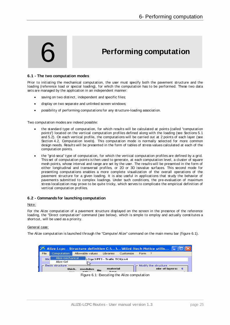
For the Alize computation of a pavement structure displayed on the screen in the presence of the reference loading, the "Direct computation" command (see below), which is simple to employ and actually constitutes a shortcut, will be used as a priority. General case:
The Alize computation is launched through the "Compute/Alize" command on the main menu bar (figure 6.1).
Figure 6.1: Executing the Alize computation
6- Performing computation
ALIZE-LCPC Routes - User manual version 1.3 page 26
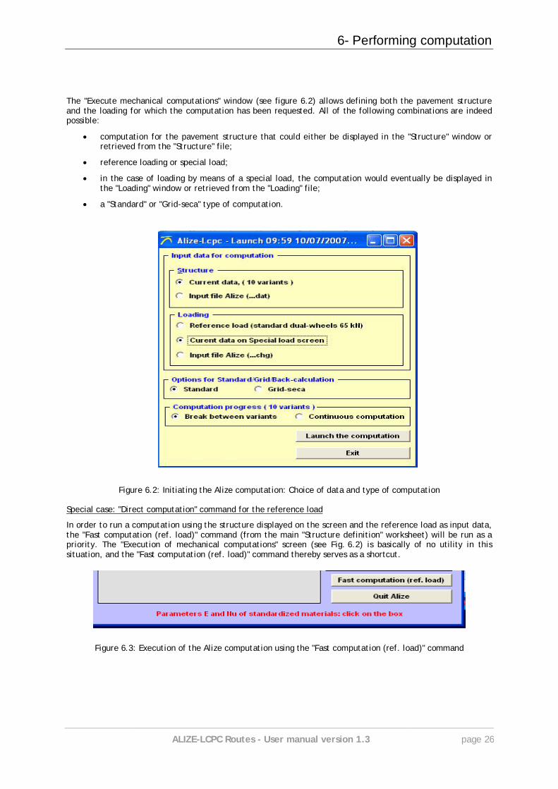
The "Execute mechanical computations" window (see figure 6.2) allows defining both the pavement structure and the loading for which the computation has been requested. All of the following combinations are indeed possible:
computation for the pavement structure that could either be displayed in the "Structure" window or retrieved from the "Structure" file;
reference loading or special load;
in the case of loading by means of a special load, the computation would eventually be displayed in the "Loading" window or retrieved from the "Loading" file;
a "Standard" or "Grid-seca" type of computation.
Figure 6.2: Initiating the Alize computation: Choice of data and type of computation Special case: "Direct computation" command for the reference load
In order to run a computation using the structure displayed on the screen and the reference load as input data, the "Fast computation (ref. load)" command (from the main "Structure definition" worksheet) will be run as a priority. The "Execution of mechanical computations" screen (see Fig. 6.2) is basically of no utility in this situation, and the "Fast computation (ref. load)" command thereby serves as a shortcut.
Figure 6.3: Execution of the Alize computation using the "Fast computation (ref. load)" command
6- Performing computation
ALIZE-LCPC Routes - User manual version 1.3 page 27
6.3 - Execution of computation in the Grid-seca mode
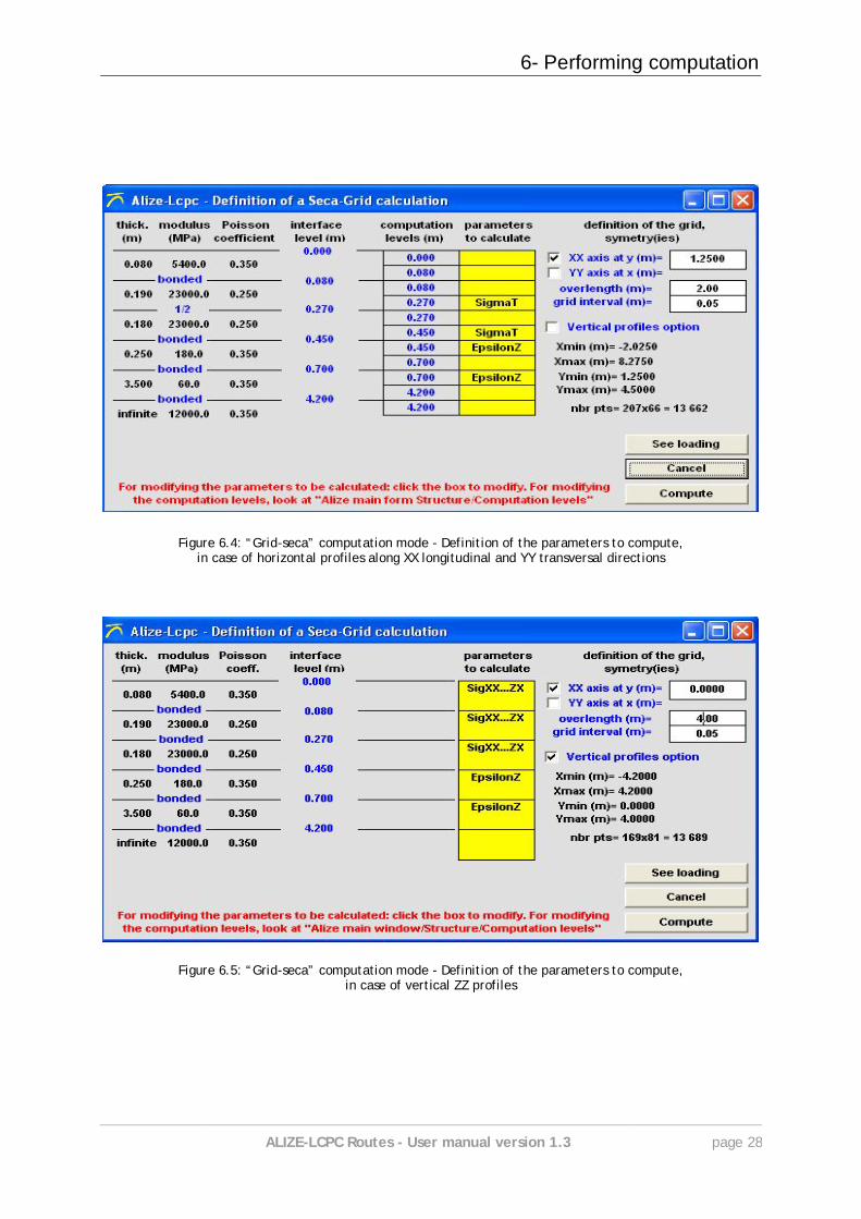
When the Grid-seca computation mode has been selected, the "Execute Alize computation" command from the "Execution of mechanical computations" screen does not directly activate the Alize computation engine, as is the case when operating in the standard computation mode. The Grid-seca computation actually relies upon the supplemental data that have been defined using the "Definition of a Grid-seca computation" window (cf. figures 6.4, 6.5 and 6.6). The supplemental data necessary for running the computations are as follows (see figures 6.4 and 6.5):
grid parameterization: in a grid-seca computation situation, the points on the XoY plane that outline the computation profiles create a cluster of rectangular points, as characterized by grid length, width and the dimensions of its elementary mesh, which serve to designate the grid "interval". The Alize program automatically proposes a computation grid on the basis of the loading geometry (either reference load or special load). The user can then modify, if so desired, this initial grid by means of altering the following parameters:
– Grid symmetries: It would be possible to deactivate the eventual symmetries inherent in the
grid; – Border: This element represents the distance between the grid boundaries and the center of
the closest load. The overhang is identical everywhere along the XX and YY directions; – Interval: the grid interval directly influences the number of computation profiles, the amount
of memory required and the Alize computation time. For purposes of illustration, the maximum grid size is approximately 850,000 computation profiles on a P3 type of PC, with 128 megabytes of RAM.
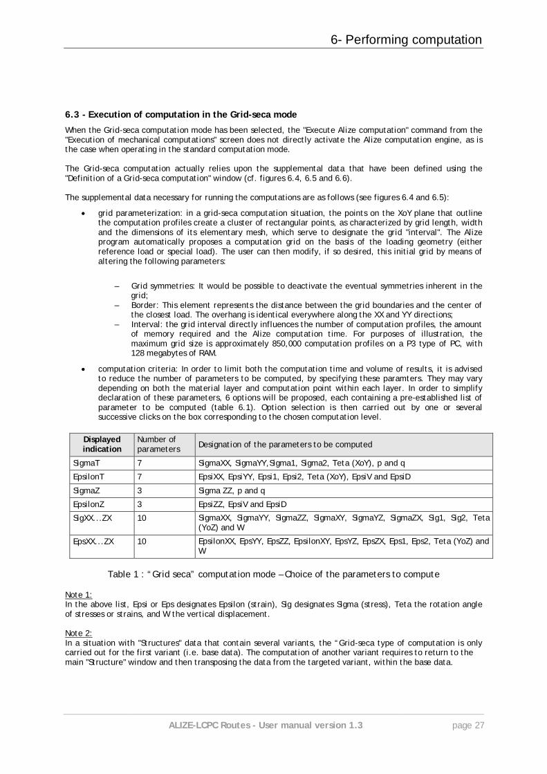
computation criteria: In order to limit both the computation time and volume of results, it is advised to reduce the number of parameters to be computed, by specifying these paramters. They may vary depending on both the material layer and computation point within each layer. In order to simplify declaration of these parameters, 6 options will be proposed, each containing a pre-established list of parameter to be computed (table 6.1). Option selection is then carried out by one or several successive clicks on the box corresponding to the chosen computation level.
Displayed indication
Number of parameters Designation of the parameters to be computed
SigmaT 7 SigmaXX, SigmaYY,Sigma1, Sigma2, Teta (XoY), p and q
EpsilonT 7 EpsiXX, EpsiYY, Epsi1, Epsi2, Teta (XoY), EpsiV and EpsiD
SigmaZ 3 Sigma ZZ, p and q
EpsilonZ 3 EpsiZZ, EpsiV and EpsiD
SigXX...ZX 10 SigmaXX, SigmaYY, SigmaZZ, SigmaXY, SigmaYZ, SigmaZX, Sig1, Sig2, Teta (YoZ) and W
EpsXX...ZX 10 EpsilonXX, EpsYY, EpsZZ, EpsilonXY, EpsYZ, EpsZX, Eps1, Eps2, Teta (YoZ) and W
Table 1 : “Grid seca” computation mode – Choice of the parameters to compute
Note 1: In the above list, Epsi or Eps designates Epsilon (strain), Sig designates Sigma (stress), Teta the rotation angle of stresses or strains, and W the vertical displacement. Note 2: In a situation with "Structures" data that contain several variants, the “Grid-seca type of computation is only carried out for the first variant (i.e. base data). The computation of another variant requires to return to the main "Structure" window and then transposing the data from the targeted variant, within the base data.
6- Performing computation
ALIZE-LCPC Routes - User manual version 1.3 page 28
Figure 6.4: “Grid-seca” computation mode - Definition of the parameters to compute, in case of horizontal profiles along XX longitudinal and YY transversal directions
Figure 6.5: “Grid-seca” computation mode - Definition of the parameters to compute, in case of vertical ZZ profiles
6- Performing computation
ALIZE-LCPC Routes - User manual version 1.3 page 29
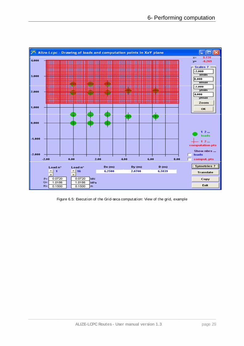
Figure 6.5: Execution of the Grid-seca computation: View of the grid, example


7- Results from the mechanical computation
ALIZE-LCPC Routes - User manual version 1.3 page 31
7
7. Results of mechanical computation
7.1 - Results from standard computation
The results from computation conducted according to the standard mode are presented on the "Mechanical computation results" screen. It is possible to print out all or part of these results, as well as to proceed with their recording onto a file.
"Results" window:
This screen primarily features the following:
a review of the structure serving as the object of the computation; the loading identifier used for the computation is also recalled herein;
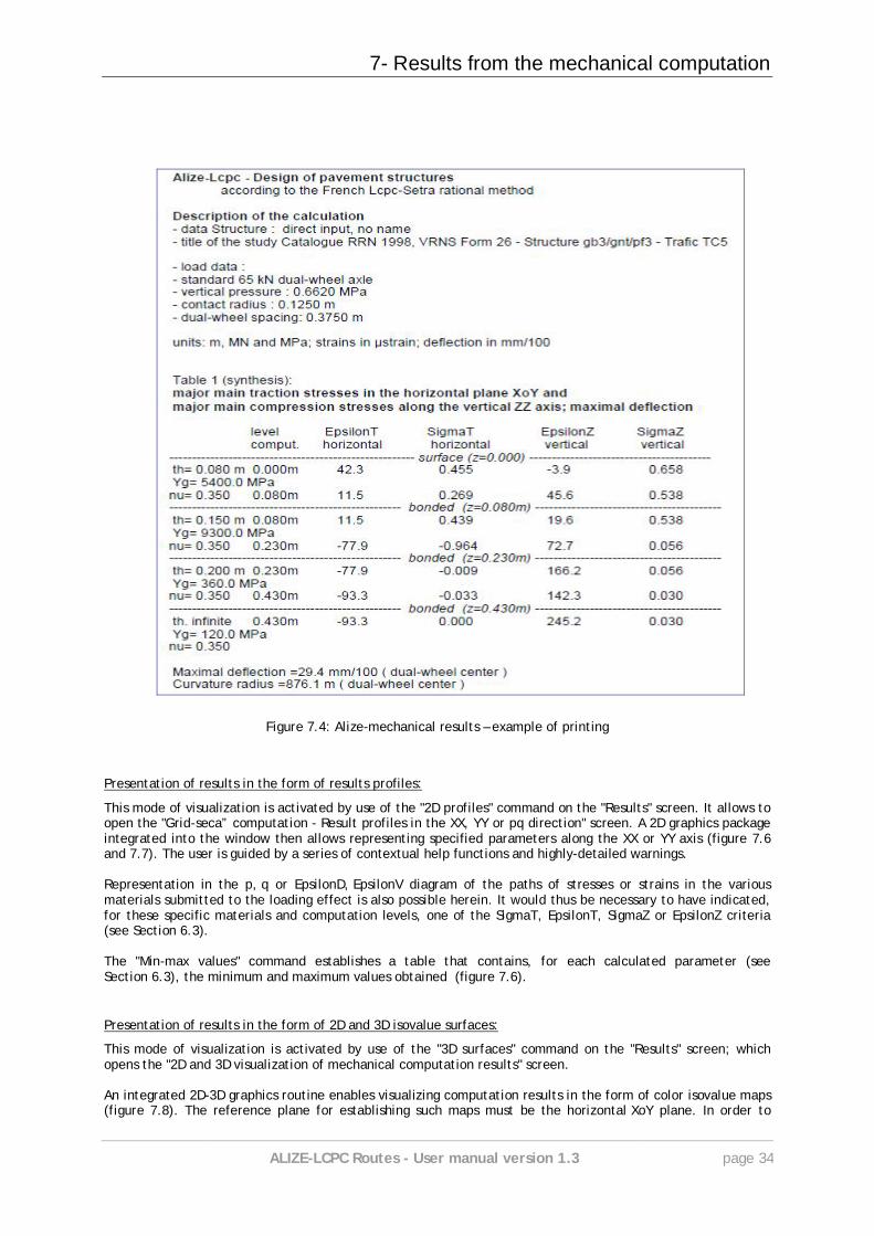
a total of 8 tables, displayed one by one, presenting the following set of results:
Table 1: Stresses and strains at the computation points. At each computation level, the minimum strain value (EpsT) and minor primary stress value (SigmaT) within the horizontal plane XoY, along with the maximum values of both strain (EpsZ) and stress (SigmaZ) in the ZZ direction. In more common design applications, this table serves to summarize the set of results used for directly designing the structure. Table 2: Stresses and strains at the computation points. Localization and orientation of the minimum EpsT and SigmaT values in the XoY plane, as well as the maximum EpsZ and SigmaZ values in the ZZ direction, as listed in Table 1. The notations used here are the following:
– - in the case of computations with the reference load: R = wheel axis, J = twinning axis, m = non-oriented XX or YY direction (stress rotation), see Table 8;
– - in the case of a special loading: Pk = vertical computation profile n°k, m = non-oriented XX or YY direction (stress rotation), see Table 8.
Table 3: Strains in the XX, YY and ZZ directions, at each computation level and at the selected vertical computation profile (see the choice of profile displayed using the vertical profile cursor). Table 4: Stresses in the XX, YY and ZZ directions, at each computation level and at the selected vertical computation profile. Table 5: Shear strains XY, YZ and ZX at each computation level and at the selected vertical computation profile. Table 6: Shear stresses XY, YZ and ZX at each computation level and at the selected vertical computation profile. Table 7: Primary major and minor strains within the XoY plane, and angle of rotation with the XX axis. Values calculated at each computation level and at the selected vertical computation profile. Table 8: Primary major and minor stresses within the XoY plane, and angle of rotation with the XX axis. Values calculated at each computation level and at the selected vertical computation profile.
7- Results from the mechanical computation
ALIZE-LCPC Routes - User manual version 1.3 page 32
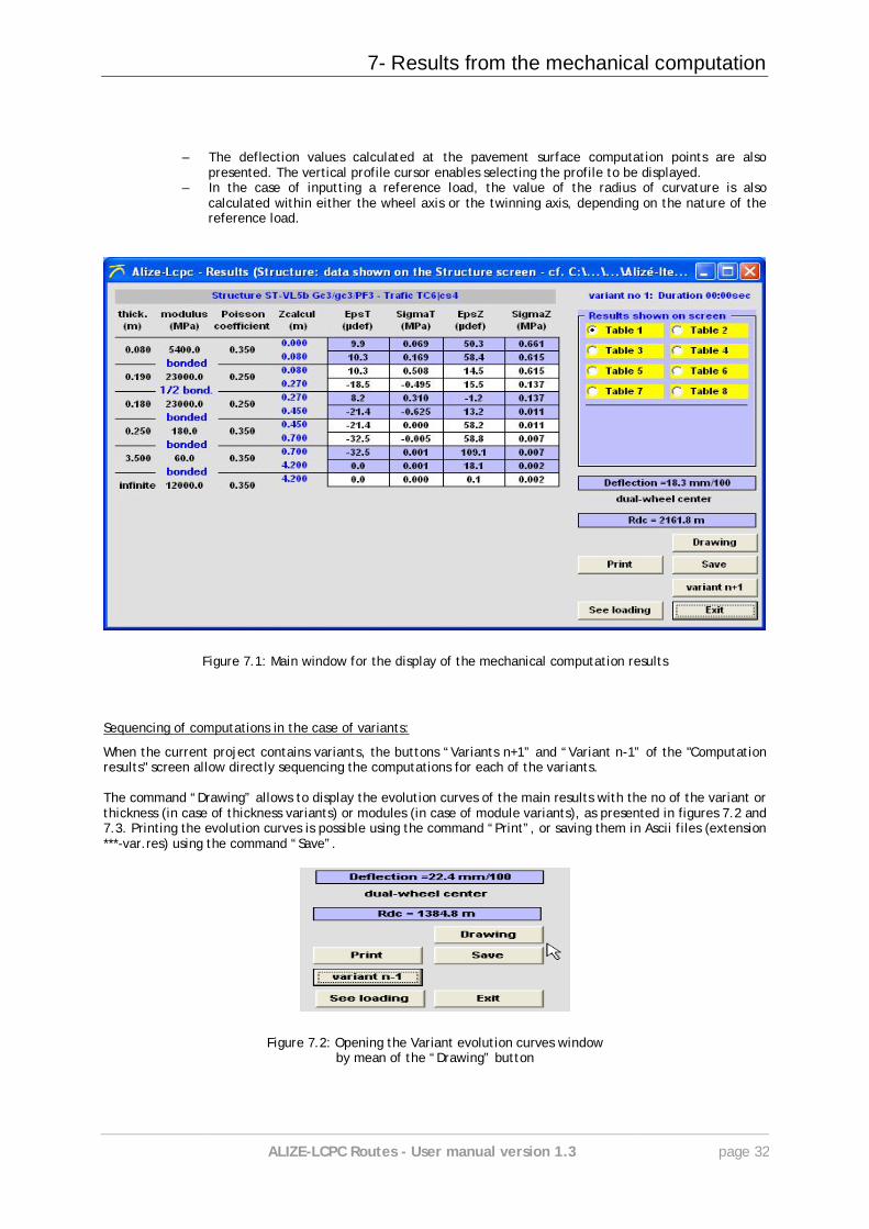
– The deflection values calculated at the pavement surface computation points are also
presented. The vertical profile cursor enables selecting the profile to be displayed. – In the case of inputting a reference load, the value of the radius of curvature is also
calculated within either the wheel axis or the twinning axis, depending on the nature of the reference load.
Figure 7.1: Main window for the display of the mechanical computation results
Sequencing of computations in the case of variants:
When the current project contains variants, the buttons “Variants n+1” and “Variant n-1” of the "Computation results" screen allow directly sequencing the computations for each of the variants. The command “Drawing” allows to display the evolution curves of the main results with the no of the variant or thickness (in case of thickness variants) or modules (in case of module variants), as presented in figures 7.2 and 7.3. Printing the evolution curves is possible using the command “Print”, or saving them in Ascii files (extension ***-var.res) using the command “Save”.
Figure 7.2: Opening the Variant evolution curves window by mean of the “Drawing” button
7- Results from the mechanical computation
ALIZE-LCPC Routes - User manual version 1.3 page 33
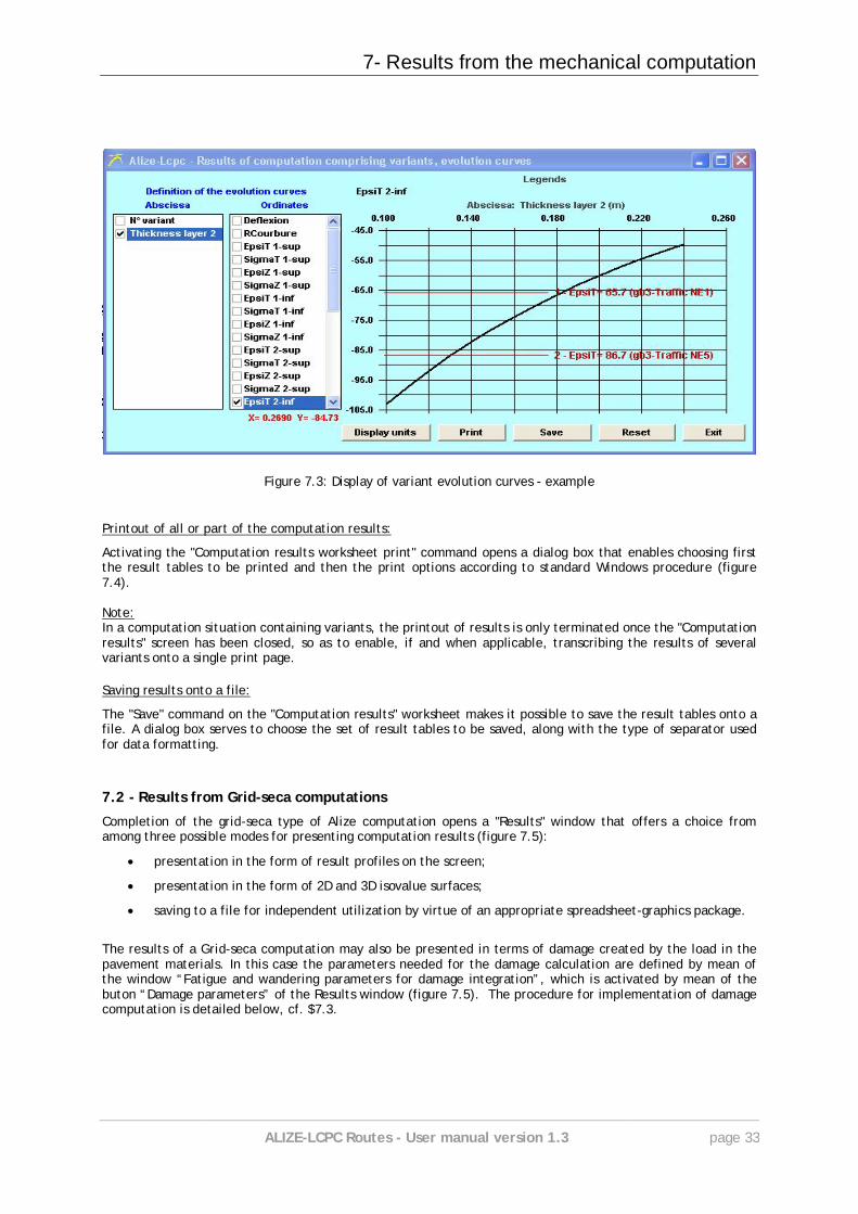
Figure 7.3: Display of variant evolution curves - example
Printout of all or part of the computation results:
Activating the "Computation results worksheet print" command opens a dialog box that enables choosing first the result tables to be printed and then the print options according to standard Windows procedure (figure 7.4). Note: In a computation situation containing variants, the printout of results is only terminated once the "Computation results" screen has been closed, so as to enable, if and when applicable, transcribing the results of several variants onto a single print page.
Saving results onto a file:
The "Save" command on the "Computation results" worksheet makes it possible to save the result tables onto a file. A dialog box serves to choose the set of result tables to be saved, along with the type of separator used for data formatting.
7.2 - Results from Grid-seca computations
Completion of the grid-seca type of Alize computation opens a "Results" window that offers a choice from among three possible modes for presenting computation results (figure 7.5):
presentation in the form of result profiles on the screen;
presentation in the form of 2D and 3D isovalue surfaces;
saving to a file for independent utilization by virtue of an appropriate spreadsheet-graphics package.
The results of a Grid-seca computation may also be presented in terms of damage created by the load in the pavement materials. In this case the parameters needed for the damage calculation are defined by mean of the window “Fatigue and wandering parameters for damage integration”, which is activated by mean of the buton “Damage parameters” of the Results window (figure 7.5). The procedure for implementation of damage computation is detailed below, cf. $7.3.
7- Results from the mechanical computation
ALIZE-LCPC Routes - User manual version 1.3 page 34
Figure 7.4: Alize-mechanical results – example of printing
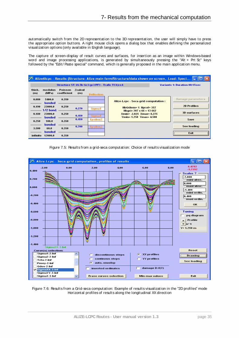
Presentation of results in the form of results profiles:
This mode of visualization is activated by use of the "2D profiles" command on the "Results" screen. It allows to open the "Grid-seca” computation - Result profiles in the XX, YY or pq direction" screen. A 2D graphics package integrated into the window then allows representing specified parameters along the XX or YY axis (figure 7.6 and 7.7). The user is guided by a series of contextual help functions and highly-detailed warnings. Representation in the p, q or EpsilonD, EpsilonV diagram of the paths of stresses or strains in the various materials submitted to the loading effect is also possible herein. It would thus be necessary to have indicated, for these specific materials and computation levels, one of the SigmaT, EpsilonT, SigmaZ or EpsilonZ criteria (see Section 6.3). The "Min-max values" command establishes a table that contains, for each calculated parameter (see Section 6.3), the minimum and maximum values obtained (figure 7.6).
Presentation of results in the form of 2D and 3D isovalue surfaces:
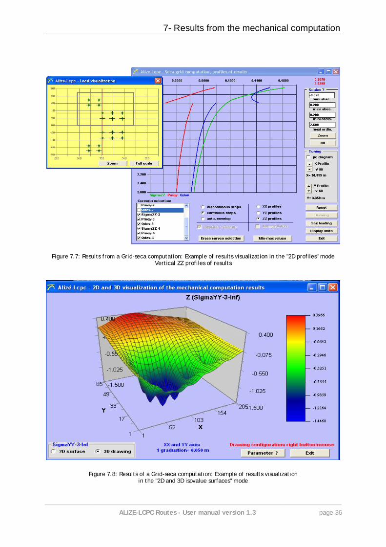
This mode of visualization is activated by use of the "3D surfaces" command on the "Results" screen; which opens the "2D and 3D visualization of mechanical computation results" screen. An integrated 2D-3D graphics routine enables visualizing computation results in the form of color isovalue maps (figure 7.8). The reference plane for establishing such maps must be the horizontal XoY plane. In order to
7- Results from the mechanical computation
ALIZE-LCPC Routes - User manual version 1.3 page 35
automatically switch from the 2D representation to the 3D representation, the user will simply have to press the appropriate option buttons. A right mouse click opens a dialog box that enables defining the personalized visualization options (only available in English language). The capture of screen-display of result curves and surfaces, for insertion as an image within Windows-based word and image processing applications, is generated by simultaneously pressing the "Alt + Prt Sc" keys followed by the "Edit/Paste special" command, which is generally proposed in the main application menu.
Figure 7.5: Results from a grid-seca computation: Choice of results visualization mode
Figure 7.6: Results from a Grid-seca computation: Example of results visualization in the "2D profiles" mode Horizontal profiles of results along the longitudinal XX direction
7- Results from the mechanical computation
ALIZE-LCPC Routes - User manual version 1.3 page 36
Figure 7.7: Results from a Grid-seca computation: Example of results visualization in the "2D profiles" mode Vertical ZZ profiles of results
Figure 7.8: Results of a Grid-seca computation: Example of results visualization in the "2D and 3D isovalue surfaces" mode
7- Results from the mechanical computation
ALIZE-LCPC Routes - User manual version 1.3 page 37
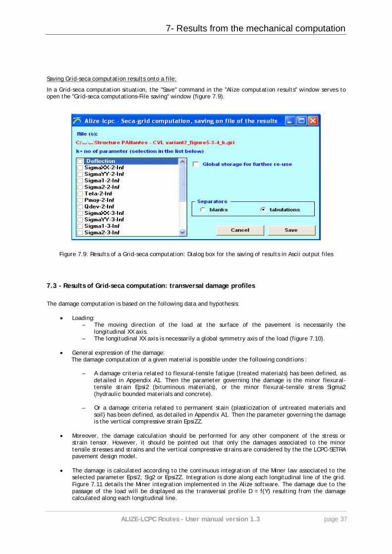
Saving Grid-seca computation results onto a file:
In a Grid-seca computation situation, the "Save" command in the "Alize computation results" window serves to open the "Grid-seca computations-File saving" window (figure 7.9).
Figure 7.9: Results of a Grid-seca computation: Dialog box for the saving of results in Ascii output files
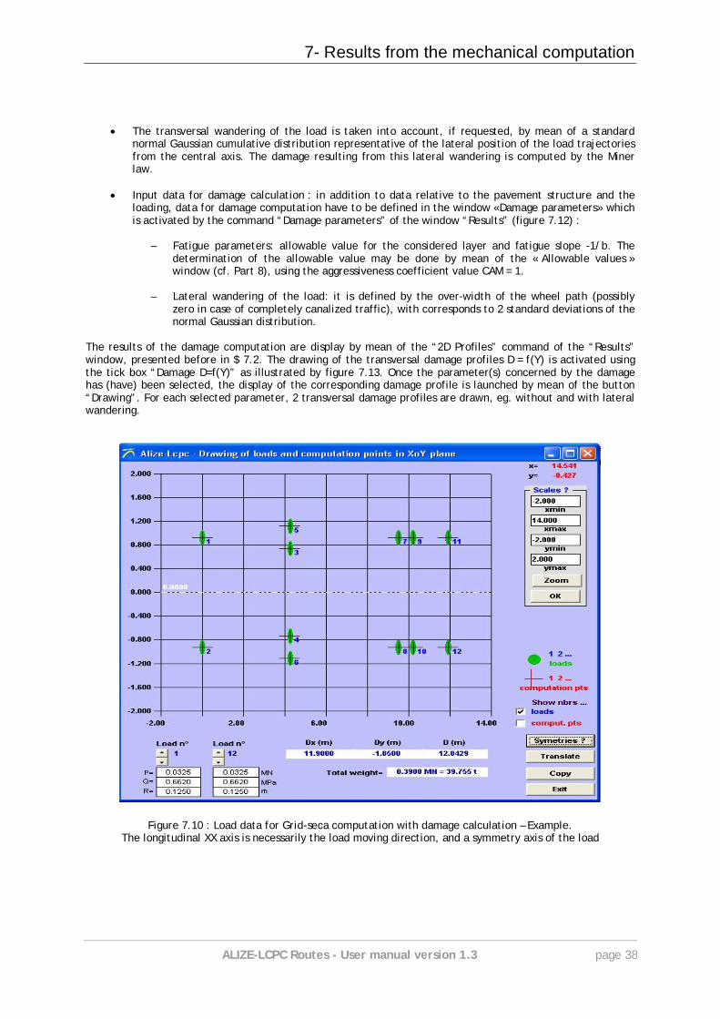
7.3 - Results of Grid-seca computation: transversal damage profiles
The damage computation is based on the following data and hypothesis:
Loading: – The moving direction of the load at the surface of the pavement is necessarily the
longitudinal XX axis. – The longitudinal XX axis is necessarily a global symmetry axis of the load (figure 7.10).
General expression of the damage:
The damage computation of a given material is possible under the following conditions :
– A damage criteria related to flexural-tensile fatigue (treated materials) has been defined, as detailed in Appendix A1. Then the parameter governing the damage is the minor flexural-tensile strain Epsi2 (bituminous materials), or the minor flexural-tensile stress Sigma2 (hydraulic bounded materials and concrete).
– Or a damage criteria related to permanent stain (plasticization of untreated materials and
soil) has been defined, as detailed in Appendix A1. Then the parameter governing the damage is the vertical compressive strain EpsiZZ.
Moreover, the damage calculation should be performed for any other component of the stress or
strain tensor. However, it should be pointed out that only the damages associated to the minor tensile stresses and strains and the vertical compressive strains are considered by the the LCPC-SETRA pavement design model.
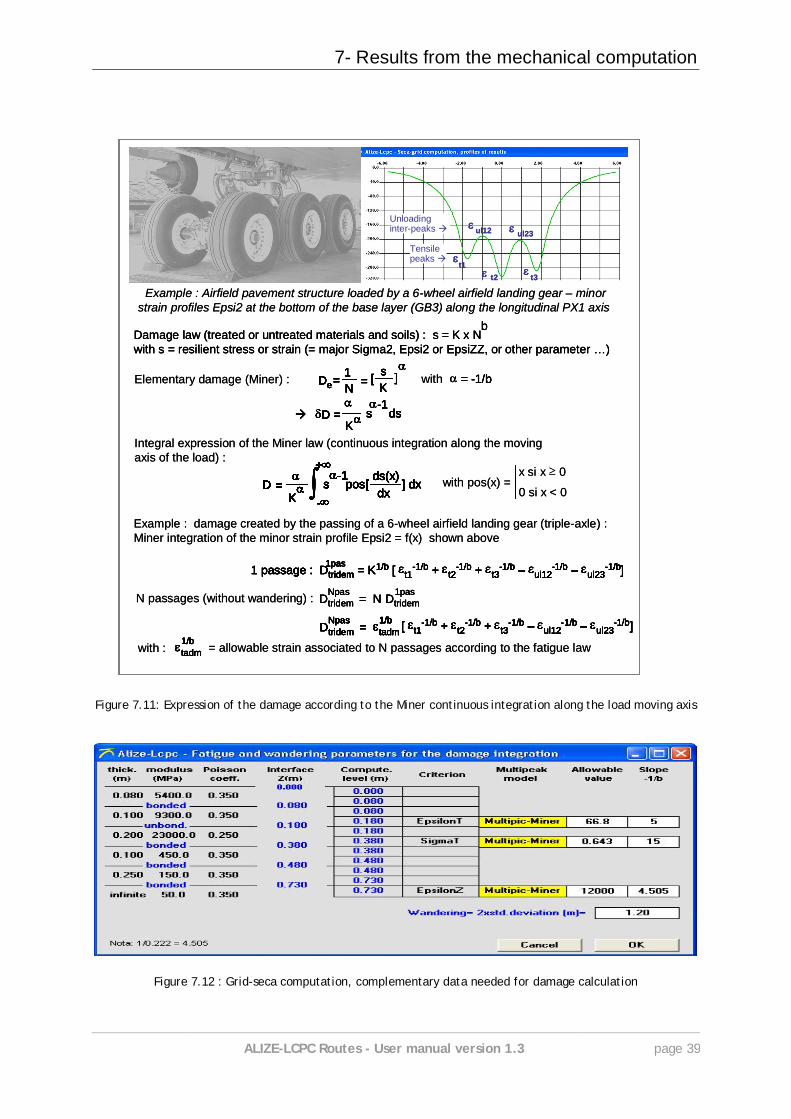
The damage is calculated according to the continuous integration of the Miner law associated to the
selected parameter Epsi2, Sig2 or EpsiZZ. Integration is done along each longitudinal line of the grid. Figure 7.11 details the Miner integration implemented in the Alize software. The damage due to the passage of the load will be displayed as the transversal profile D = f(Y) resulting from the damage calculated along each longitudinal line.
7- Results from the mechanical computation
ALIZE-LCPC Routes - User manual version 1.3 page 38
The transversal wandering of the load is taken into account, if requested, by mean of a standard
normal Gaussian cumulative distribution representative of the lateral position of the load trajectories from the central axis. The damage resulting from this lateral wandering is computed by the Miner law.
Input data for damage calculation : in addition to data relative to the pavement structure and the
loading, data for damage computation have to be defined in the window «Damage parameters» which is activated by the command “Damage parameters” of the window “Results” (figure 7.12) :
– Fatigue parameters: allowable value for the considered layer and fatigue slope -1/b. The
determination of the allowable value may be done by mean of the « Allowable values » window (cf. Part 8), using the aggressiveness coefficient value CAM = 1.
– Lateral wandering of the load: it is defined by the over-width of the wheel path (possibly
zero in case of completely canalized traffic), with corresponds to 2 standard deviations of the normal Gaussian distribution.
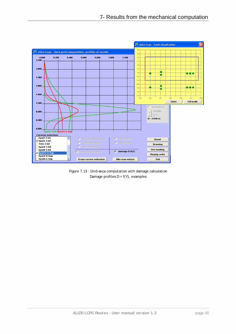
The results of the damage computation are display by mean of the “2D Profiles” command of the “Results” window, presented before in $ 7.2. The drawing of the transversal damage profiles D = f(Y) is activated using the tick box “Damage D=f(Y)” as illustrated by figure 7.13. Once the parameter(s) concerned by the damage has (have) been selected, the display of the corresponding damage profile is launched by mean of the button “Drawing”. For each selected parameter, 2 transversal damage profiles are drawn, eg. without and with lateral wandering.
Figure 7.10 : Load data for Grid-seca computation with damage calculation – Example. The longitudinal XX axis is necessarily the load moving direction, and a symmetry axis of the load
7- Results from the mechanical computation
ALIZE-LCPC Routes - User manual version 1.3 page 39
t1
t2 t3
Pics detraction
ul12ul23
Déchargementinter-pic
Example : Airfield pavement structure loaded by a 6-wheel airfield landing gear – minorstrain profiles Epsi2 at the bottom of the base layer (GB3) along the longitudinal PX1 axis
= -1/bDe= 1N =
sK
]
[
pos[ ] dxds(x)dx
D = -
+
Ks-1
D = s ds-1
K
1 passage : Dtridem = K1/b [ t1-1/b + t2
-1/b + t3-1/b – ul12
-1/b – ul23-1/b] 1pas
Dtridem = tadm [ t1-1/b + t2
-1/b + t3-1/b – ul12
-1/b – ul23-1/b] Npas 1/b
Integral expression of the Miner law (continuous integration along the movingaxis of the load) :
Example : damage created by the passing of a 6-wheel airfield landing gear (triple-axle) :Miner integration of the minor strain profile Epsi2 = f(x) shown above
t1
t1 t2 t2 t3 t3
Tensilepeaks
ul12 ul12ul23 ul23
Unloadinginter-peaks
Elementary damage (Miner) : with = -1/bDe= 1N =
sK
]
[De= 1N =
sK
]
[
bDamage law (treated or untreated materials and soils) : s = K x Nwith s = resilient stress or strain (= major Sigma2, Epsi2 or EpsiZZ, or other parameter …)
x si x 0
0 si x < 0 pos[ ] dx
ds(x)dx
D = -
+
Ks-1
with pos(x) =pos[ ] dxds(x)dx
D = -
+
Ks-1
pos[ ] dxds(x)dx
D = -
+
Ks-1
D = -
+
Ks-1
D = s ds-1
K D = s ds
-1
K
Dtridem = N DtridemNpas 1pasN passages (without wandering) : Dtridem = N DtridemNpas 1pas
1 passage : Dtridem = K1/b [ t1-1/b + t2
-1/b + t3-1/b – ul12
-1/b – ul23-1/b] 1pas1 passage : Dtridem = K1/b [ t1
-1/b + t2-1/b + t3
-1/b – ul12-1/b – ul23
-1/b] 1pas
Dtridem = [ t1-1/b + t2
-1/b + t3-1/b – ul12
-1/b – ul23-1/b] Npas
Dtridem = [ t1-1/b + t2
-1/b + t3-1/b – ul12
-1/b – ul23-1/b] Npas tadm
1/btadm1/b
with : tadm1/btadm1/b = allowable strain associated to N passages according to the fatigue law
t1
t1 t2 t2 t3 t3
Pics detraction
ul12 ul12ul23 ul23
Déchargementinter-pic
Example : Airfield pavement structure loaded by a 6-wheel airfield landing gear – minorstrain profiles Epsi2 at the bottom of the base layer (GB3) along the longitudinal PX1 axis
= -1/bDe= 1N =
sK
]
[De= 1N =
sK
]
[
pos[ ] dxds(x)dx
D = -
+
Ks-1
pos[ ] dxds(x)dx
D = -
+
Ks-1
D = -
+
Ks-1
D = s ds-1
K D = s ds
-1
K
1 passage : Dtridem = K1/b [ t1-1/b + t2
-1/b + t3-1/b – ul12
-1/b – ul23-1/b] 1pas1 passage : Dtridem = K1/b [ t1
-1/b + t2-1/b + t3
-1/b – ul12-1/b – ul23
-1/b] 1pas
Dtridem = tadm [ t1-1/b + t2
-1/b + t3-1/b – ul12
-1/b – ul23-1/b] Npas 1/b
Dtridem = tadm [ t1-1/b + t2
-1/b + t3-1/b – ul12
-1/b – ul23-1/b] Npas 1/b
Integral expression of the Miner law (continuous integration along the movingaxis of the load) :
Example : damage created by the passing of a 6-wheel airfield landing gear (triple-axle) :Miner integration of the minor strain profile Epsi2 = f(x) shown above
t1
t1 t2 t2 t3 t3
Tensilepeaks
ul12 ul12ul23 ul23
Unloadinginter-peaks
Elementary damage (Miner) : with = -1/bDe= 1N =
sK
]
[De= 1N =
sK
]
[
bDamage law (treated or untreated materials and soils) : s = K x Nwith s = resilient stress or strain (= major Sigma2, Epsi2 or EpsiZZ, or other parameter …)
bDamage law (treated or untreated materials and soils) : s = K x Nwith s = resilient stress or strain (= major Sigma2, Epsi2 or EpsiZZ, or other parameter …)
x si x 0
0 si x < 0 pos[ ] dx
ds(x)dx
D = -
+
Ks-1
pos[ ] dxds(x)dx
D = -
+
Ks-1
D = -
+
Ks-1
with pos(x) =pos[ ] dxds(x)dx
D = -
+
Ks-1
D = -
+
Ks-1
pos[ ] dxds(x)dx
D = -
+
Ks-1
D = -
+
Ks-1
D = s ds-1
K D = s ds
-1
K
Dtridem = N DtridemNpas 1pasN passages (without wandering) : Dtridem = N DtridemNpas 1pas
1 passage : Dtridem = K1/b [ t1-1/b + t2
-1/b + t3-1/b – ul12
-1/b – ul23-1/b] 1pas1 passage : Dtridem = K1/b [ t1
-1/b + t2-1/b + t3
-1/b – ul12-1/b – ul23
-1/b] 1pas
Dtridem = [ t1-1/b + t2
-1/b + t3-1/b – ul12
-1/b – ul23-1/b] Npas
Dtridem = [ t1-1/b + t2
-1/b + t3-1/b – ul12
-1/b – ul23-1/b] Npas tadm
1/btadm1/btadm1/btadm1/b
with : tadm1/btadm1/btadm1/btadm1/b = allowable strain associated to N passages according to the fatigue law
Figure 7.11: Expression of the damage according to the Miner continuous integration along the load moving axis
Figure 7.12 : Grid-seca computation, complementary data needed for damage calculation
7- Results from the mechanical computation
ALIZE-LCPC Routes - User manual version 1.3 page 40
Figure 7.13 : Grid-seca computation with damage calculation Damage profiles D = f(Y), examples
8- Computation of allowable values
ALIZE-LCPC Routes - User manual version 1.3 page 41
8
8. Computation of allowable values
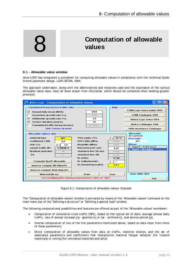
8.1 - Allowable value window
Alize-LCPC has integrated a worksheet for computing allowable values in compliance with the technical Guide French pavement design, LCPC-SETRA, 1994. The approach undertaken, along with the abbreviations and notations used and the expression of the various allowable value laws, have all been drawn from this Guide, which should be consulted when seeking greater precision.
Figure 8.1: Computation of allowable values: Example The "Computation of allowable values" window is activated by means of the "Allowable values" command on the main menu bar of the "Defining a structure" or "Defining a special load" window. The following computational possibilities and features are offered as part of the "Allowable values" worksheet:
Computation of cumulative truck traffic (NPL), based on the typical set of data: average annual daily traffic, rate of annual increase (tg - geometric) or (at - arithmetic), and service period (p);
Inverse computation of two of the five parameters mentioned above, based on data input from three of these parameters;
Direct computation of allowable values from data on traffic, material choices, and the set of associated parameters and coefficients that characterize material fatigue behavior (for treated materials) or rutting (for untreated materials and soils);
8- Computation of allowable values
ALIZE-LCPC Routes - User manual version 1.3 page 42
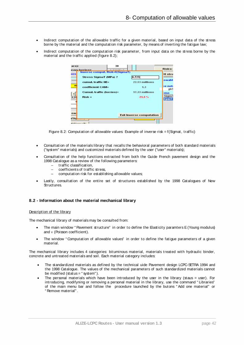
Indirect computation of the allowable traffic for a given material, based on input data of the stress borne by the material and the computation risk parameter, by means of inverting the fatigue law;
Indirect computation of the computation risk parameter, from input data on the stress borne by the material and the traffic applied (figure 8.2);
Figure 8.2: Computation of allowable values: Example of inverse risk = f(Sigmat, traffic)
Consultation of the materials library that recalls the behavioral parameters of both standard materials ("system" materials) and customized materials defined by the user ("user" materials);
Consultation of the help functions extracted from both the Guide French pavement design and the 1998 Catalogue as a review of the following parameters:
– traffic classification, – coefficients of traffic stress, – computation risk for establishing allowable values;
Lastly, consultation of the entire set of structures established by the 1998 Catalogues of New Structures.
8.2 - Information about the material mechanical library
Description of the library The mechanical library of materials may be consulted from:
The main window “Pavement structure” in order to define the Elasticity paramters E (Young modulus) and (Poisson coefficient).
The window “Computation of allowable values” in order to define the fatigue parameters of a given material.
The mechanical library includes 4 categories: bituminous material, materials treated with hydraulic binder, concrete and untreated materials and soil. Each material category includes:
The standardized materials as defined by the technical uide Pavement design LCPC-SETRA 1994 and the 1998 Catalogue. The values of the mechanical parameters of such standardized materials cannot be modified (status = “system”).
The personal materials which have been introduced by the user in the library (staus = user). For introducing, modifyning or removing a personal material in the library, use the command “Libraries” of the main menu bar and follow the procedure launched by the butons “Add one material” or “Remove material”.
8- Computation of allowable values
ALIZE-LCPC Routes - User manual version 1.3 page 43
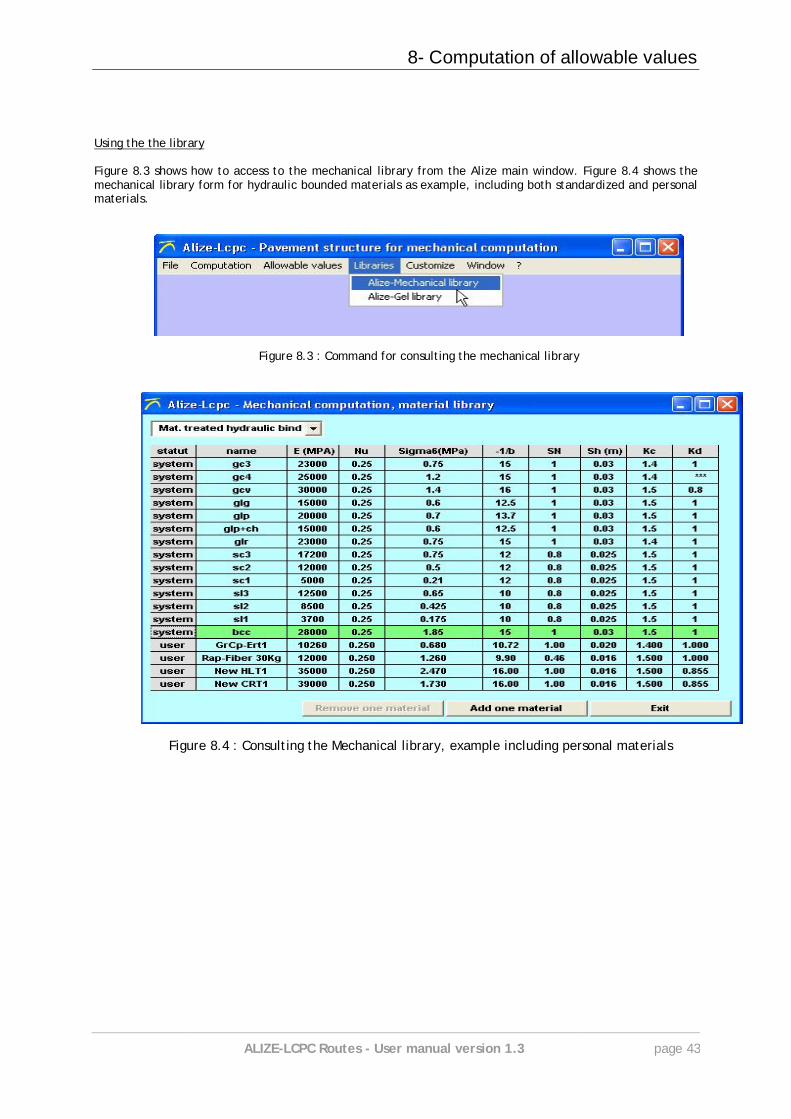
Using the the library
Figure 8.3 shows how to access to the mechanical library from the Alize main window. Figure 8.4 shows the mechanical library form for hydraulic bounded materials as example, including both standardized and personal materials.
Figure 8.3 : Command for consulting the mechanical library
Figure 8.4 : Consulting the Mechanical library, example including personal materials


9- Alize-Frost thaw : Data preparation
ALIZE-LCPC Routes - User manual version 1.3 page 45
9
9. Alize-Frost thaw: Data preparation
9.1 - Description of the problem
For the Alize-frost computation, the pavement is represented by a mono-directional multilayered structure, made up of finite thickness homogeneous layers reproducing both the pavement structure and the subgrade. In common practice, the total thickness of the model is always more than twenty or thirty meters, so that the temperature at the bottom of the model may be considered as constant; not depending on the time. For instance, the Lcpc-Setra rational design method specifies that the bottom of the model is located 40 meters above the top of the capping layer (also called the foundation layer in this manual). As for the mechanical computation, the thickness of each layer of the Frost-thaw model is assumed to be constant, and its lateral extension in the horizontal plane XoY is infinite (mono-directional model assumptions). Each layer is defined by the following parameters:
Thickness H ;
Voluminal mass ;
Water content of the material ;
Thermal conductibility of the material in unfrosted situation ;
Thermal conductibility of the material in frost situation. The computation also requests initial and boundary temperature conditions:
The initial temperature condition is given by the vertical temperature profile at the time t=0, defined as a multi-linear profile Temperature = function (depth).
The boundary conditions are given at the top and at the bottom of the model, by mean of two multi-linear relationships Temperature = function (time). These boundary conditions constitute the thermal loading of the model.
The Alize-frost computation kernel calculates the evolution with the time, of the temperature at the surface of the model and at each interface level between adjacent layers. Theses results are also presented in the terms of the evolution curves in the time of the frost quantity at the same levels, and frost index at the surface of the pavement. The surface frost index is converted into atmospheric index. In the majority of cases, the finalized result of frost computation is presented in term of the frost index allowable by a given pavement structure (main unknown of the problem to solve), depending on the frost quantity transmitted at the top of the capping layer. This frost quantity transmitted at the top of the capping layer is an input of the problem. It can be evaluated by mean of a specific help-sheet included in the Alize-frost module, accordingly to the Lcpc-Setra ‘s design Guide. The evolution with the time of the frost front depth (s) is (are) also calculated and edited. Alize-frost is based on a finite differences algorithm, which unknown parameters are the temperature and the frost front depth speed. Three different thermal behaviour areas are considered:
The unfrosted area, which the thermal equilibrium follows from the heat equation without source term ;
The frost area, which is characterized by thermal behaviour parameters different from the unfrosted area ;
9- Alize-Frost thaw : Data preparation
ALIZE-LCPC Routes - User manual version 1.3 page 46
The frost front(s), which is (are) separating surface(s) between the unfrosted and the frost areas. Latent heat absorption/dissipation phenomena develop on the frost front(s), which therefore present thermal gradient discontinuity.
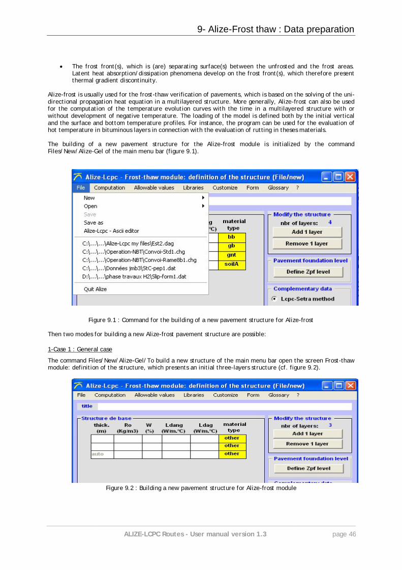
Alize-frost is usually used for the frost-thaw verification of pavements, which is based on the solving of the uni-directional propagation heat equation in a multilayered structure. More generally, Alize-frost can also be used for the computation of the temperature evolution curves with the time in a multilayered structure with or without development of negative temperature. The loading of the model is defined both by the initial vertical and the surface and bottom temperature profiles. For instance, the program can be used for the evaluation of hot temperature in bituminous layers in connection with the evaluation of rutting in theses materials. The building of a new pavement structure for the Alize-frost module is initialized by the command Files/New/Alize-Gel of the main menu bar (figure 9.1).
Figure 9.1 : Command for the building of a new pavement structure for Alize-frost
Then two modes for building a new Alize-frost pavement structure are possible:
1-Case 1 : General case
The command Files/New/Alize-Gel/To build a new structure of the main menu bar open the screen Frost-thaw module: definition of the structure, which presents an initial three-layers structure (cf. figure 9.2).
Figure 9.2 : Building a new pavement structure for Alize-frost module
9- Alize-Frost thaw : Data preparation
ALIZE-LCPC Routes - User manual version 1.3 page 47
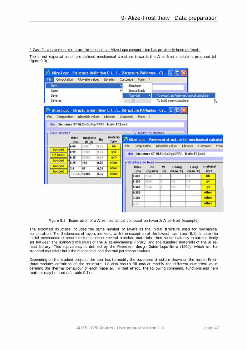
2-Case 2 : a pavement structure for mechanical Alize-Lcpc computation has previously been defined :
The direct exportation of pre-defined mechanical structure towards the Alize-frost module is proposed (cf. figure 9.3).
Figure 9.3 : Exportation of a Alize mechanical computation towards Alize-frost (example)
The exported structure includes the same number of layers as the initial structure used for mechanical computation. The thicknesses of layers are kept, with the exception of the lowest layer (see §9.2). In case the initial mechanical structure includes one or several standard materials, then an equivalency is automatically set between the standard materials of the Alize-mechanical library, and the standard materials of the Alize-frost library. This equivalency is defined by the Pavement design Guide Lcpc-Setra (1994), which set for standard materials both the mechanical and thermal parameters values. Depending on the studied project, the user has to modify the pavement structure shown on the screen Frost-thaw module: definition of the structure. He also has to fill and/or modify the different numerical value defining the thermal behaviour of each material. To that effect, the following command, functions and help routines may be used (cf. table 9.1) :
9- Alize-Frost thaw : Data preparation
ALIZE-LCPC Routes - User manual version 1.3 page 48
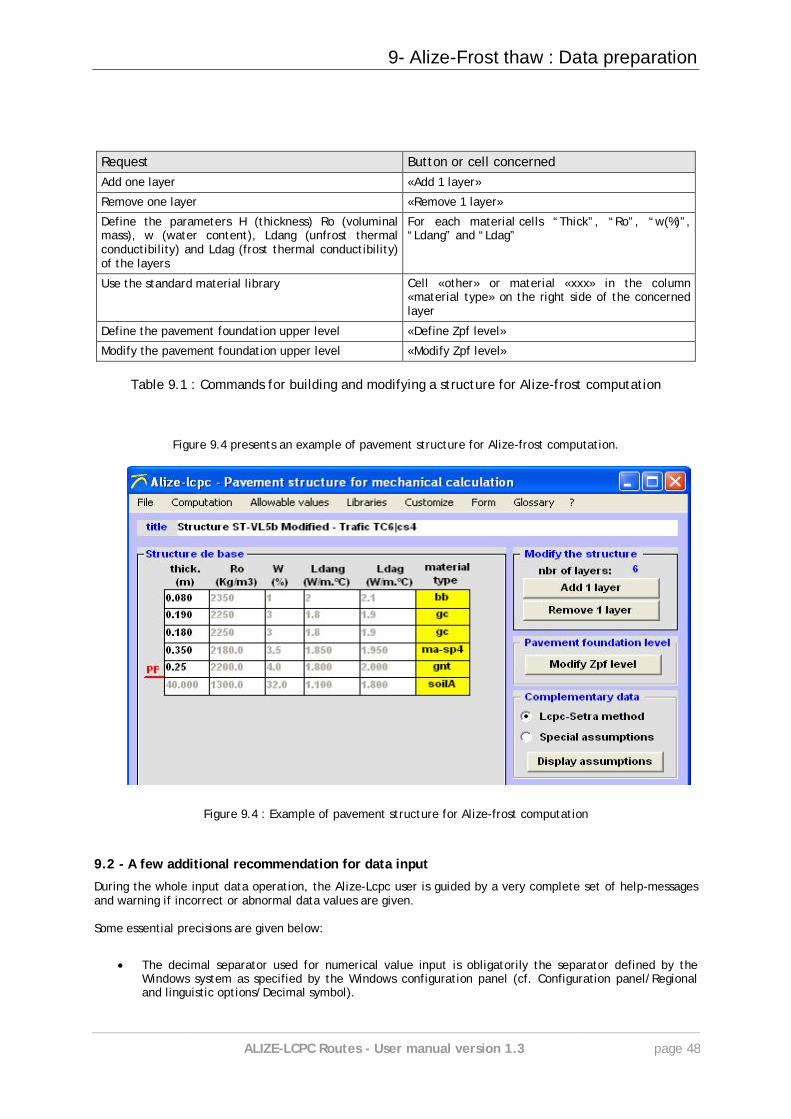
Request Button or cell concerned Add one layer «Add 1 layer»
Remove one layer «Remove 1 layer»
Define the parameters H (thickness) Ro (voluminal mass), w (water content), Ldang (unfrost thermal conductibility) and Ldag (frost thermal conductibility) of the layers
For each material cells “Thick”, “Ro”, “w(%)”, “Ldang” and “Ldag”
Use the standard material library Cell «other» or material «xxx» in the column «material type» on the right side of the concerned layer
Define the pavement foundation upper level «Define Zpf level»
Modify the pavement foundation upper level «Modify Zpf level»
Table 9.1 : Commands for building and modifying a structure for Alize-frost computation
Figure 9.4 presents an example of pavement structure for Alize-frost computation.
Figure 9.4 : Example of pavement structure for Alize-frost computation
9.2 - A few additional recommendation for data input During the whole input data operation, the Alize-Lcpc user is guided by a very complete set of help-messages and warning if incorrect or abnormal data values are given. Some essential precisions are given below:
The decimal separator used for numerical value input is obligatorily the separator defined by the Windows system as specified by the Windows configuration panel (cf. Configuration panel/Regional and linguistic options/Decimal symbol).
9- Alize-Frost thaw : Data preparation
ALIZE-LCPC Routes - User manual version 1.3 page 49
It is recommended to give a title to the data (cf. Title line), in order to later facilitate its identification, for instance as the data are again read on file in further Alize sessions, or as the computation results are edited.
The lowest layer thickness is not directly given by the user. It is automatically calculated by the program, from:
– The upper level Zpf of the pavement foundation in case of standard initial and boundary conditions (cf. Lcpc-Setra ‘s rational design method, frost-thaw verification §9.4) ;
– The total thickness of the model defined by the vertical initial temperature profile To=f(z), in case of special initial and/or boundary condition different from the Lcpc-Setra ones (cf. §9.4).
The number of layers making up the whole pavement structure (including soil) is limited to 15. The minimal number is 2.
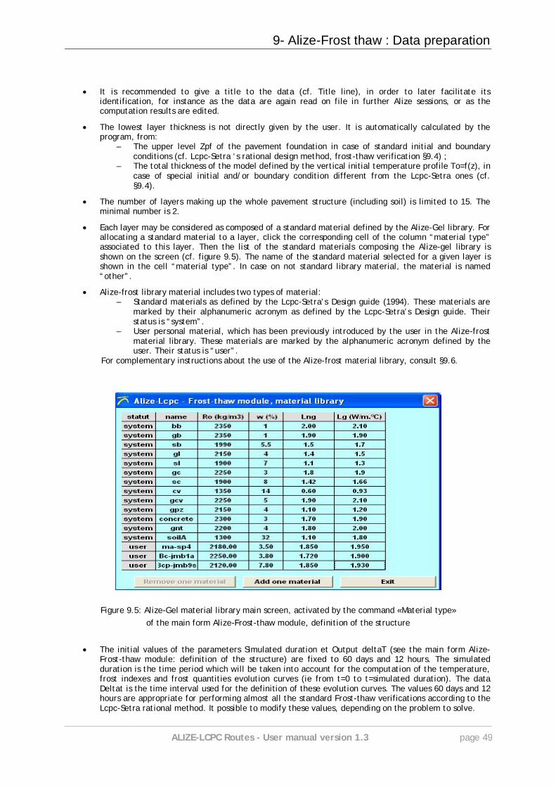
Each layer may be considered as composed of a standard material defined by the Alize-Gel library. For allocating a standard material to a layer, click the corresponding cell of the column “material type” associated to this layer. Then the list of the standard materials composing the Alize-gel library is shown on the screen (cf. figure 9.5). The name of the standard material selected for a given layer is shown in the cell “material type”. In case on not standard library material, the material is named “other”.
Alize-frost library material includes two types of material: – Standard materials as defined by the Lcpc-Setra’s Design guide (1994). These materials are
marked by their alphanumeric acronym as defined by the Lcpc-Setra’s Design guide. Their status is “system”.
– User personal material, which has been previously introduced by the user in the Alize-frost material library. These materials are marked by the alphanumeric acronym defined by the user. Their status is “user”.
For complementary instructions about the use of the Alize-frost material library, consult §9.6.
Figure 9.5: Alize-Gel material library main screen, activated by the command «Material type» of the main form Alize-Frost-thaw module, definition of the structure
The initial values of the parameters Simulated duration et Output deltaT (see the main form Alize-Frost-thaw module: definition of the structure) are fixed to 60 days and 12 hours. The simulated duration is the time period which will be taken into account for the computation of the temperature, frost indexes and frost quantities evolution curves (ie from t=0 to t=simulated duration). The data Deltat is the time interval used for the definition of these evolution curves. The values 60 days and 12 hours are appropriate for performing almost all the standard Frost-thaw verifications according to the Lcpc-Setra rational method. It possible to modify these values, depending on the problem to solve.

9- Alize-Frost thaw : Data preparation
ALIZE-LCPC Routes - User manual version 1.3 page 50
9.3 - Saving and reading of data files
After a pavement structure for Alize-frost thaw computation has been completely defined, and before going on and launching the computation, it is recommended to save the data defining this structure. For saving on screen data, use the command Files/Save as of the main menu bar of the main Alize-Lcpc Frost sheet. The saving on file is operated by mean of the classical Windows Save on file dialog box. The commands Files/Open and Files/Save are used for reading and saving data in existing data files. They are also operated by mean of the standard Windows dialog boxes.
9.4 - Definition of initial and boundary conditions The definition of the vertical initial and boundary temperature conditions has obligatorily to be done before launching the computation. This condition are defined by mean of the tick boxes of the frame Complementary data of the main sheet Alize-Frost-thaw module: definition of the structure. Two modes are proposed for the initial and boundary condition definition: Assumptions of the Lcpc-Setra Design method : The choice Lcpc-Sétra method lead to select the initial and boundary conditions of the Lcpc-Setra Frost-thaw verification method, as defined by the Lcpc-Setra Design guide (1994). If this first option is ticked, then the command Display assumption of the frame Complementary activates the visualization on screen of these conditions (cf. figure 9.6).
Figure 9.6: Visualization of the initial vertical temperature profile and the upper and lower boundary condition temperature evolution curves, as defined by the Lcpc-Setra Design Guide (1994)
Special assumptions: If the option Special assumptions is ticked, then the command Define-change-display of the frame Complementary data open the sheet Alize-Lcpc Frost-thaw, special assumptions.
This sheet is used for defining initial and boundary conditions different from the conditions specified by the Lcpc-Setra Frost-thaw verification method. An example of such special temperature initial and boundary conditions is shown on the figure 9.7.
9- Alize-Frost thaw : Data preparation
ALIZE-LCPC Routes - User manual version 1.3 page 51
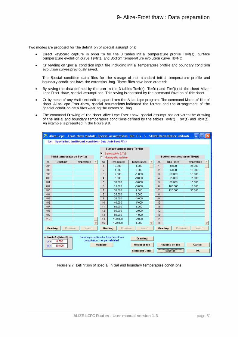
Two modes are proposed for the definition of special assumptions:
Direct keyboard capture in order to fill the 3 tables Initial temperature profile To=f(z), Surface temperature evolution curve Ts=f(t), and Bottom temperature evolution curve Tb=f(t).
Or reading on Special condition input file including initial temperature profile and boundary condition evolution curves previously saved. The Special condition data files for the storage of not standard initial temperature profile and boundary conditions have the extension .hag. These files have been created:
By saving the data defined by the user in the 3 tables To=f(z), Ts=f(t) and Tb=f(t) of the sheet Alize-Lcpc Frost-thaw, special assumptions. This saving is operated by the command Save on of this sheet.
Or by mean of any Ascii text editor, apart from the Alize-Lcpc program. The command Model of file of sheet Alize-Lcpc Frost-thaw, special assumptions indicated the format and the arrangement of the Special condition data files wearing the extension .hag.
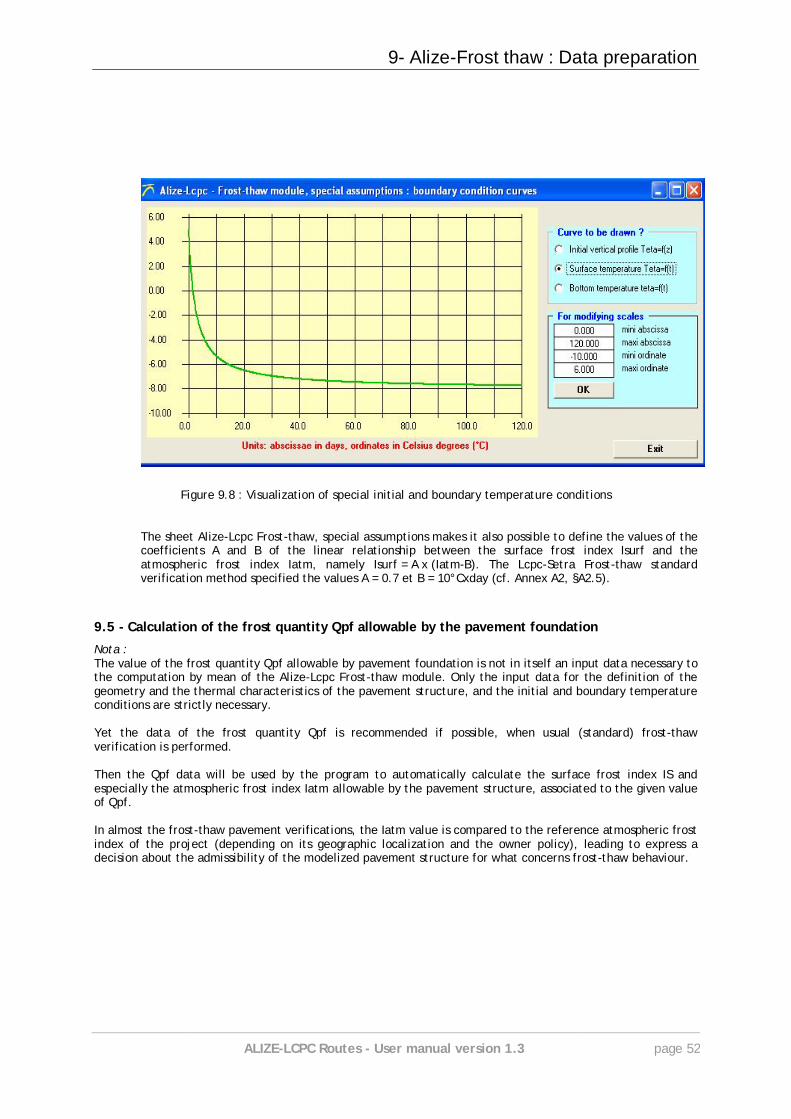
The command Drawing of the sheet Alize-Lcpc Frost-thaw, special assumptions activates the drawing of the initial and boundary temperature conditions defined by the tables To=f(t), Ts=f(t) and Tb=f(t). An example is presented in the figure 9.8.
Figure 9.7: Definition of special initial and boundary temperature conditions
9- Alize-Frost thaw : Data preparation
ALIZE-LCPC Routes - User manual version 1.3 page 52
Figure 9.8 : Visualization of special initial and boundary temperature conditions The sheet Alize-Lcpc Frost-thaw, special assumptions makes it also possible to define the values of the coefficients A and B of the linear relationship between the surface frost index Isurf and the atmospheric frost index Iatm, namely Isurf = A x (Iatm-B). The Lcpc-Setra Frost-thaw standard verification method specified the values A = 0.7 et B = 10°Cxday (cf. Annex A2, §A2.5).
9.5 - Calculation of the frost quantity Qpf allowable by the pavement foundation Nota : The value of the frost quantity Qpf allowable by pavement foundation is not in itself an input data necessary to the computation by mean of the Alize-Lcpc Frost-thaw module. Only the input data for the definition of the geometry and the thermal characteristics of the pavement structure, and the initial and boundary temperature conditions are strictly necessary. Yet the data of the frost quantity Qpf is recommended if possible, when usual (standard) frost-thaw verification is performed. Then the Qpf data will be used by the program to automatically calculate the surface frost index IS and especially the atmospheric frost index Iatm allowable by the pavement structure, associated to the given value of Qpf. In almost the frost-thaw pavement verifications, the Iatm value is compared to the reference atmospheric frost index of the project (depending on its geographic localization and the owner policy), leading to express a decision about the admissibility of the modelized pavement structure for what concerns frost-thaw behaviour.
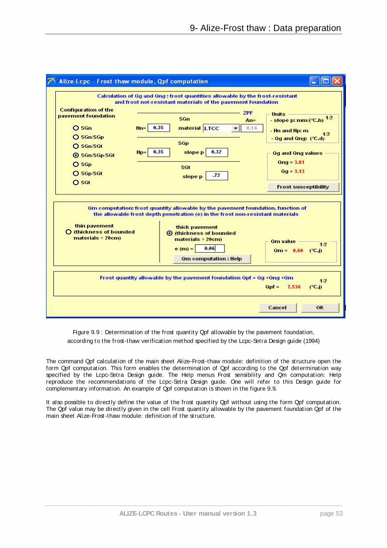
9- Alize-Frost thaw : Data preparation
ALIZE-LCPC Routes - User manual version 1.3 page 53
Figure 9.9 : Determination of the frost quantity Qpf allowable by the pavement foundation, according to the frost-thaw verification method specified by the Lcpc-Setra Design guide (1994)
The command Qpf calculation of the main sheet Alize-Frost-thaw module: definition of the structure open the form Qpf computation. This form enables the determination of Qpf according to the Qpf determination way specified by the Lcpc-Setra Design guide. The Help menus Frost sensibility and Qm computation: Help reproduce the recommendations of the Lcpc-Setra Design guide. One will refer to this Design guide for complementary information. An example of Qpf computation is shown in the figure 9.9. It also possible to directly define the value of the frost quantity Qpf without using the form Qpf computation. The Qpf value may be directly given in the cell Frost quantity allowable by the pavement foundation Qpf of the main sheet Alize-Frost-thaw module: definition of the structure.
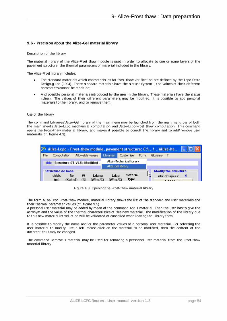
9- Alize-Frost thaw : Data preparation
ALIZE-LCPC Routes - User manual version 1.3 page 54
9.6 - Precision about the Alize-Gel material library
Description of the library The material library of the Alize-Frost thaw module is used in order to allocate to one or some layers of the pavement structure, the thermal parameters of material included in the library. The Alize-Frost library includes:
The standard materials which characteristics for frost-thaw verification are defined by the Lcpc-Setra Design guide (1994). These standard materials have the status “System”, the values of their different parameters cannot be modified;
And possible personal materials introduced by the user in the library. These materials have the status «User». The values of their different parameters may be modified. It is possible to add personal materials to the library, and to remove them.
Use of the library The command Libraries/Alize-Gel library of the main menu may be launched from the main menu bar of both the main sheets Alize-Lcpc mechanical computation and Alize-Lcpc-Frost thaw computation. This command opens the Frost-thaw material library, and makes it possible to consult the library and to add/remove user materials (cf. figure 4.3).
Figure 4.3: Opening the Frost-thaw material library The form Alize-Lcpc Frost-thaw module, material library shows the list of the standard and user materials and their thermal parameter values (cf. figure 9.5). A personal user material may be added by mean of the command Add 1 material. Then the user has to give the acronym and the value of the thermal characteristics of this new material. The modification of the library due to this new material introduction will be validated or cancelled when leaving the Library form. It is possible to modify the name and/or the parameter values of a personal user material. For selecting the user material to modify, use a left mouse-click on the material to be modified, then the content of the different cells may be changed. The command Remove 1 material may be used for removing a personnel user material from the Frost-thaw material library.
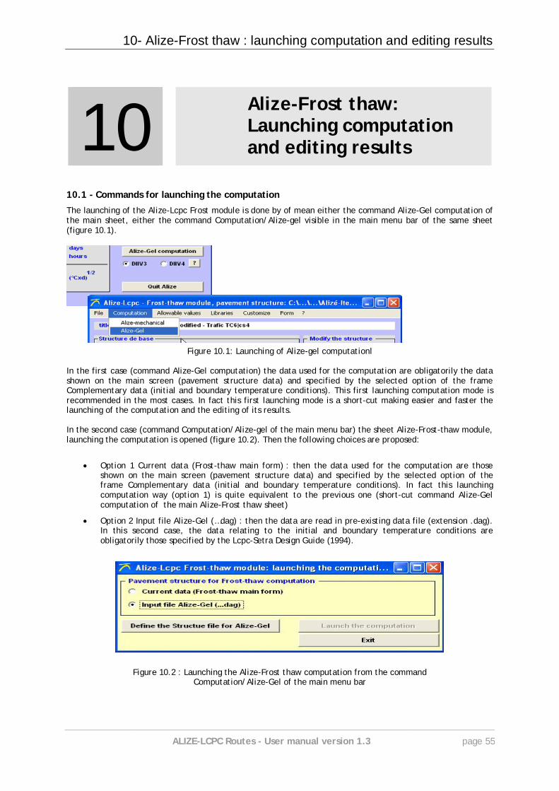
10- Alize-Frost thaw : launching computation and editing results
ALIZE-LCPC Routes - User manual version 1.3 page 55
10
10. Alize-Frost thaw: Launching computation and editing results
10.1 - Commands for launching the computation
The launching of the Alize-Lcpc Frost module is done by of mean either the command Alize-Gel computation of the main sheet, either the command Computation/Alize-gel visible in the main menu bar of the same sheet (figure 10.1).
Figure 10.1: Launching of Alize-gel computationl
In the first case (command Alize-Gel computation) the data used for the computation are obligatorily the data shown on the main screen (pavement structure data) and specified by the selected option of the frame Complementary data (initial and boundary temperature conditions). This first launching computation mode is recommended in the most cases. In fact this first launching mode is a short-cut making easier and faster the launching of the computation and the editing of its results. In the second case (command Computation/Alize-gel of the main menu bar) the sheet Alize-Frost-thaw module, launching the computation is opened (figure 10.2). Then the following choices are proposed:
Option 1 Current data (Frost-thaw main form) : then the data used for the computation are those shown on the main screen (pavement structure data) and specified by the selected option of the frame Complementary data (initial and boundary temperature conditions). In fact this launching computation way (option 1) is quite equivalent to the previous one (short-cut command Alize-Gel computation of the main Alize-Frost thaw sheet)
Option 2 Input file Alize-Gel (…dag) : then the data are read in pre-existing data file (extension .dag). In this second case, the data relating to the initial and boundary temperature conditions are obligatorily those specified by the Lcpc-Setra Design Guide (1994).
Figure 10.2 : Launching the Alize-Frost thaw computation from the command Computation/Alize-Gel of the main menu bar
10- Alize-Frost thaw : launching computation and editing results
ALIZE-LCPC Routes - User manual version 1.3 page 56
10.2 - Results of the Alize-Frost thaw computation
As soon as the computation are finished, the sheet Alize-Frost-thaw module - Computation results is automatically open. The results are presented in 5 graphs, which can be individually shown on screen according to choice done by the user. Graph 1 : Graph 1 represents the variations of surface pavement frost index (Is) and atmospheric frost index Iatm, as a function of the frost quantity Qpf transmitted at the top Zpf of the pavement foundation. This first graph also presents the variation curve Iatm=f(Qpf), resulting from the simplified method of calculation proposed by the Lcpc-Setra Design guide (1994). This last curve is presented on graph 1, providing that the two following condition are simultaneously verified:
All the materials making up the simulated pavement (including soil) are standard materials of the Frost-thaw material library (materials having the status « user », cf. §9.6.1) In the opposite case, the simplified Iatm=f(Qpf) cannot be applied, the linearization coefficients of the simplified relationship being not defined for the not-standard materials.
The option Recall the results of the simplified method must have been previously selected. This option is accessible through the Customize/Personal options of the main menu bar (cf. figure 10.3).
In case the frost quantity allowable by the pavement foundation (Qpf-adm) has been previously determined (cf. §9.5), the atmospheric frost index Iatm associated to Qpf is automatically calculated and displayed on screen. The comparison between this Iatm value and the atmospheric reference index IR is usually considered by the user, in order to express a decision about the admissibility of the modelized pavement structure for what concerns frost-thaw behaviour. Figure 10.4 presents an example of computation result curves IS = f(Qpf) and Iatm = f(Qpf).
Graph 2 : Graph 2 represents the evolution curves of frost quantity at interface between layers interfaces and pavement surface level, versus the time (cf. example shown on the figure 10.5). Graph 3 : Graph 3 represents the vertical temperature profiles calculated at 6 value of the time, uniformly distributed over the whole computation period (cf. example shown on figure 10.6). Graph 4 : Graph 4 represents the evolution curves of temperature at interface between layers and at pavement surface level, versus the time (cf. example shown on the figure 10.7). Graph 5 : Graph 5 represents the evolution curve(s) of the frost front depth(s), versus the time (cf. example shown on the figure 10.8).
The whole results of the current computation (graphs 1 to 5) may be stored in a temporary internal buffer, using the button Memo Cj of the Alize-Frost results screen (j is the number of the concerned computation, which is incremented by 1 at each launching of a new computation). Then it will possible to automatically recall these stored results and superpose them to the results of further computations, using the button Remind Cj of the Alize-Frost results screen. By this way, a direct comparison between the results of two computations using different data may be directly displayed on screen, as shown on figure 10.9. The contain of the internal buffer (results Cj) may be replaced at any moment by the results of the current computation (Ck), using the button Memo Ck of the Alize-Frost results screen.
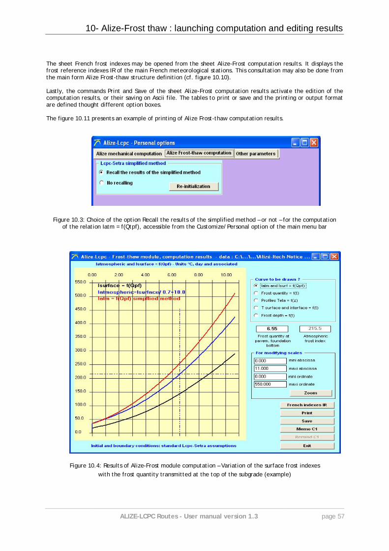
10- Alize-Frost thaw : launching computation and editing results
ALIZE-LCPC Routes - User manual version 1.3 page 57
The sheet French frost indexes may be opened from the sheet Alize-Frost computation results. It displays the frost reference indexes IR of the main French meteorological stations. This consultation may also be done from the main form Alize Frost-thaw structure definition (cf. figure 10.10).
Lastly, the commands Print and Save of the sheet Alize-Frost computation results activate the edition of the computation results, or their saving on Ascii file. The tables to print or save and the printing or output format are defined thought different option boxes. The figure 10.11 presents an example of printing of Alize Frost-thaw computation results.
Figure 10.3: Choice of the option Recall the results of the simplified method – or not – for the computation of the relation Iatm = f(Qtpf), accessible from the Customize/Personal option of the main menu bar
Figure 10.4: Results of Alize-Frost module computation – Variation of the surface frost indexes
with the frost quantity transmitted at the top of the subgrade (example)
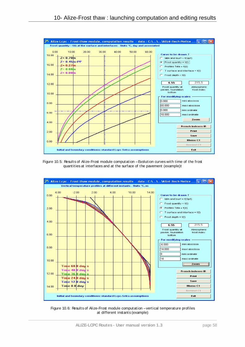
10- Alize-Frost thaw : launching computation and editing results
ALIZE-LCPC Routes - User manual version 1.3 page 58
Figure 10.5: Results of Alize-Frost module computation – Evolution curves with time of the frost
quantities at interfaces and at the surface of the pavement (example)t
Figure 10.6: Results of Alize-Frost module computation – vertical temperature profiles at different instants (example)
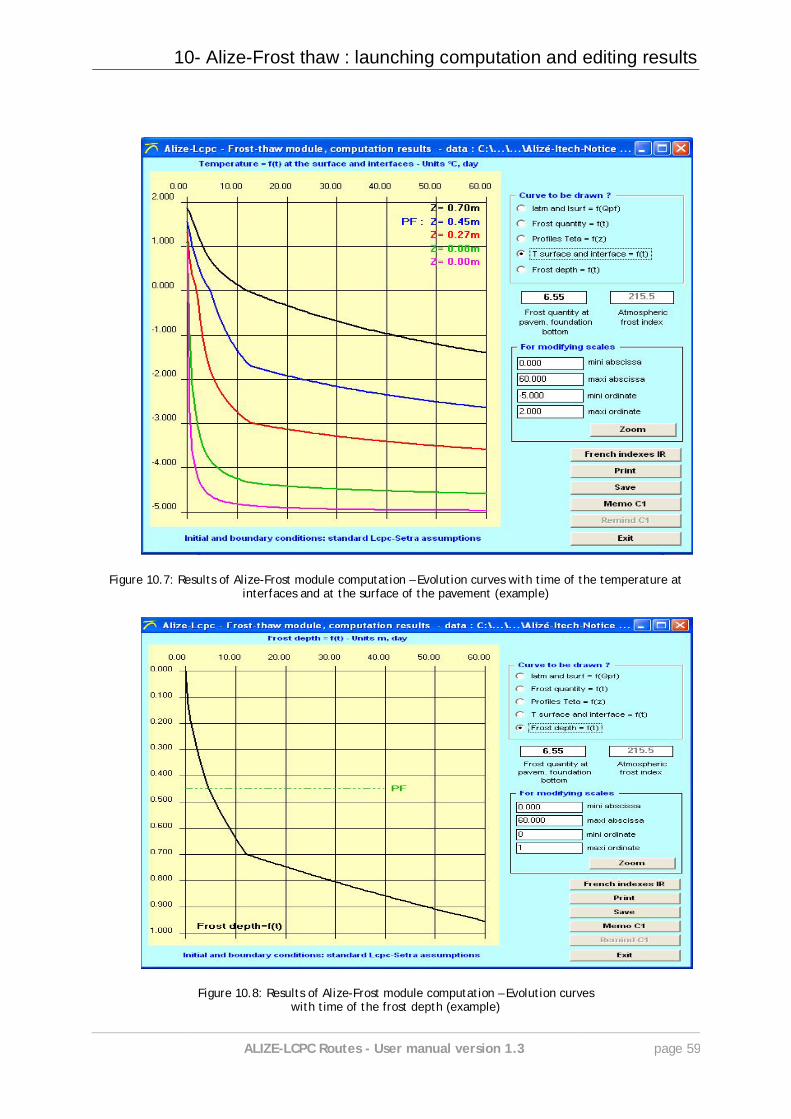
10- Alize-Frost thaw : launching computation and editing results
ALIZE-LCPC Routes - User manual version 1.3 page 59
Figure 10.7: Results of Alize-Frost module computation – Evolution curves with time of the temperature at interfaces and at the surface of the pavement (example)
Figure 10.8: Results of Alize-Frost module computation – Evolution curves with time of the frost depth (example)
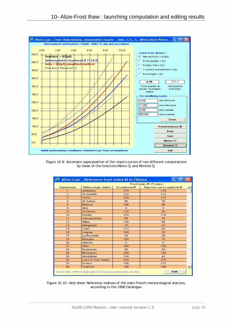
10- Alize-Frost thaw : launching computation and editing results
ALIZE-LCPC Routes - User manual version 1.3 page 60
Figure 10.9: Automatic superposition of the results curves of two different computations by mean of the functions Memo Cj and Remind Cj
Figure 10.10: Help sheet Reference indexes of the main French meteorological stations, according to the 1998 Catalogue

10- Alize-Frost thaw : launching computation and editing results
ALIZE-LCPC Routes - User manual version 1.3 page 61
Figure 10.10 : Printing of Alize Frost-thaw computation results, example

11- Alize Back-calculation: Data, computation and results
ALIZE-LCPC Routes - User manual version 1.3 page 63
11
11. Alize Back-calculation: Data, computation and results
11.1 - The problem concerned by the Alize Back-calculation module
This module of the Alize-Lcpc software allows the evaluation of the elasticity moduli of the whole or some layers of a pavement structure, from the deflection bowl created by a calibrated load. This calibrated load may consist in a single circular uniform vertical loading applied by a wheel or the plate of the FWD test device. It also may consist in the dual wheel of the Deflectometer or the Curviameter. The pavement structure is simulated by a linear multilayer structure, according to the principles and the hypothesis of the rational pavement design method implemented in the Alize software. The thickness, the Poisson’s coefficient of each layer and the interface condition between layers are known data. The unknown parameters of the problem to solve are the Young moduli of the materials. They are determined by a manual or numerical procedure, base on the optimization of the adjustment between the measured deflections and the deflections calculated by the Alize elastic-multilayer model. In common practice, the back-calculated moduli may contribute to the evaluation of the actual damage of an in-service pavement. They can also be used for determining the overlay of a damaged pavement structure. The data needed by the back-calculation procedure are as follows:
Data concerning the pavement structure: number of layers, thicknesses and Poisson’s coefficients of each layer, interface condition between layers. Initial values of the unknown elasticity moduli are also needed. Depending on the type of back-calculation to performed, these initial module values are used for initializing the numerical adjustment algorithm (Newton Raphson type), or to built the computation grid, as detailed in $11.2
Data concerning the pavement loading: type of load (single or dual), radius of the print-foot, vertical
force or uniform pressure applied, and dual-wheel spacing in the case of dual-wheel.
Deflection bowl defined by the deflection measured at several points (up to 13) located at different distances from the center of the load.
Three types of processing are proposed to the user:
Back-calculation based on the automatic optimization of the adjustment between the measured and computed deflection bowl. Then this problem of over-dimensioned system of linear equations is solved by mean of an optimized Newton-Raphson algorithm implemented in the Alize software.
Back-calculation according to a grid of moduli values defined by the user. For each layer, the series
of module values to considered are predefined (arithmetical suite) by mean of its minimal value, its arithmetic ratio, and the number of modulus values to consider. In this case, the program performs the direct computation of the deflection basin associated to each module combination. The results are finally classified in the order of decreasing adjustment precision.
Computation of the surface moduli. For a given point of deflection measure, the surface module is
defined as the Young module of the semi-infinite linear-elastic model (Boussinesq one’s) leading to the same deflection as the measured one. The curve of surface moduli may bring some contribution for the evaluation of the linear or not-linear behavior of the pavement, or even the substratum depth.
In operational application, the most frequently mode of modulus back-computation is the Newton-Raphson automatical procedure. The other two modes are generally reserved for specific application. The access to the Alize-Back calculation module is done by mean of the command ”Calculation/Alize-Back calculation” of the main menu bar (figure 11.1).
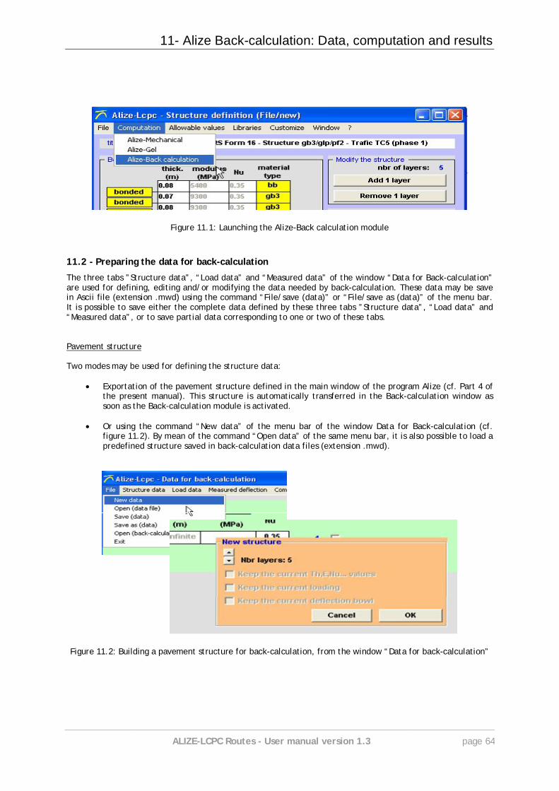
11- Alize Back-calculation: Data, computation and results
ALIZE-LCPC Routes - User manual version 1.3 page 64
Figure 11.1: Launching the Alize-Back calculation module
11.2 - Preparing the data for back-calculation
The three tabs ”Structure data”, “Load data” and “Measured data” of the window “Data for Back-calculation” are used for defining, editing and/or modifying the data needed by back-calculation. These data may be save in Ascii file (extension .mwd) using the command “File/save (data)” or “File/save as (data)” of the menu bar. It is possible to save either the complete data defined by these three tabs ”Structure data”, “Load data” and “Measured data”, or to save partial data corresponding to one or two of these tabs. Pavement structure Two modes may be used for defining the structure data:
Exportation of the pavement structure defined in the main window of the program Alize (cf. Part 4 of the present manual). This structure is automatically transferred in the Back-calculation window as soon as the Back-calculation module is activated.
Or using the command “New data” of the menu bar of the window Data for Back-calculation (cf.
figure 11.2). By mean of the command “Open data” of the same menu bar, it is also possible to load a predefined structure saved in back-calculation data files (extension .mwd).
Figure 11.2: Building a pavement structure for back-calculation, from the window “Data for back-calculation”
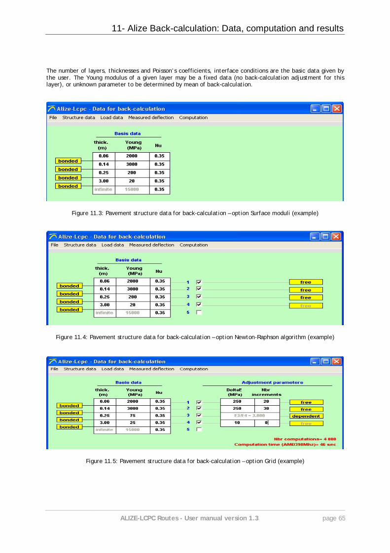
11- Alize Back-calculation: Data, computation and results
ALIZE-LCPC Routes - User manual version 1.3 page 65
The number of layers, thicknesses and Poisson’s coefficients, interface conditions are the basic data given by the user. The Young modulus of a given layer may be a fixed data (no back-calculation adjustment for this layer), or unknown parameter to be determined by mean of back-calculation.
Figure 11.3: Pavement structure data for back-calculation – option Surface moduli (example)
Figure 11.4: Pavement structure data for back-calculation – option Newton-Raphson algorithm (example)
Figure 11.5: Pavement structure data for back-calculation – option Grid (example)

11- Alize Back-calculation: Data, computation and results
ALIZE-LCPC Routes - User manual version 1.3 page 66
Figure 11.6: Loading data for back-calculation – FWD example In the first case (fixed module values), the material library may help to defined the fixed Young modulus of standardized of personal materials. In the second case (unknown Young modulus to be back-calculated), initial modulus values are requested:
If the Newton-Raphson option is selected: the initial values of Young modulus may have a significant effect on the results of the back-calculation. Moreover, the numerical solution to the optimization problem is not unique. Therefore, it is recommended to introduce initial values as close as possible to the results of the back-calculation, or close lower values, using a manual iterative approach if necessary.
If the grid option is selected, the minimal value of the modulus ranges for each material as to be
entered. Figure 11.3 presents an example of data in the case of Surface moduli back-calulation. Figure 11.4 presents an example in the case of Newton-Raphson back-calculation. Figure 11.5 presents an example in the case of grid back-calculation. In the cases of Newton-Raphson and Grid computation, the tick-box associated to each layer is used in order to specify whether the modulus of this layer has to be back-calulated or not. If not (un-ticked box), the Young modulus remains equal to the initial value given in the Structure data tab. In the case of Newton-Raphson bac-kcalculation, the tick-box “Free/dependant” associated to each layer permits to fix a dependency relationship between the modulus of the layer, and the modulus of the layer directly below. If “Dependant” condition is selected, then the ration of these two moduli will be remain constant, equal to the ration of their initial values defined in the Structure data tab. Loading data: The load used for back-calculation is defined by mean of the tab ”Load data” (figure 11.6). It may consist in a single circular uniform vertical loading applied by a wheel or the plate of the FWD or HWD test device. It also may consist in the dual wheel of the Deflectometer or the Curviameter. Deflection data: The measured deflections are entered by mean of the “Measured deflection” tab (figure 11.7).
Single deflection basin input. The parameters to enter are: The number of measure points (number of geophones in the case of FWD measure). The coordinates X, Y of the deflection points, and the measured deflections. Units are meters
(m) and mm/100.
The command “Drawing” may be used in order to draw the deflection bowl. The command “File/Open data” of the menu bar may be used in order to load any single deflection bowl previously saved.
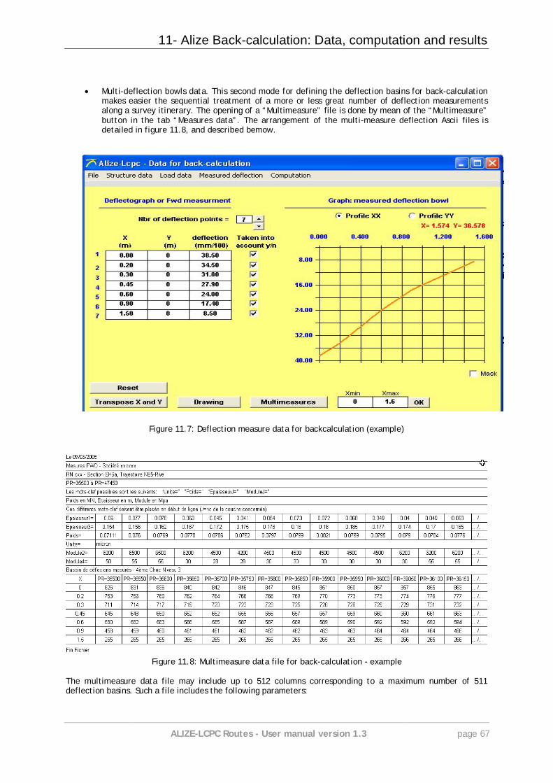
11- Alize Back-calculation: Data, computation and results
ALIZE-LCPC Routes - User manual version 1.3 page 67
Multi-deflection bowls data. This second mode for defining the deflection basins for back-calculation makes easier the sequential treatment of a more or less great number of deflection measurements along a survey itinerary. The opening of a “Multimeasure” file is done by mean of the “Multimeasure” button in the tab “Measures data”. The arrangement of the multi-measure deflection Ascii files is detailed in figure 11.8, and described bemow.
Figure 11.7: Deflection measure data for backcalculation (example)
Figure 11.8: Multimeasure data file for back-calculation - example
The multimeasure data file may include up to 512 columns corresponding to a maximum number of 511 deflection basins. Such a file includes the following parameters:
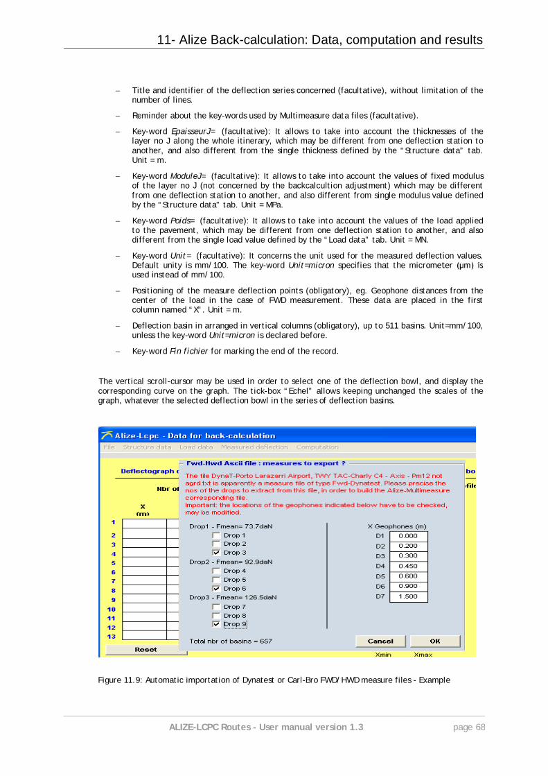
11- Alize Back-calculation: Data, computation and results
ALIZE-LCPC Routes - User manual version 1.3 page 68
Title and identifier of the deflection series concerned (facultative), without limitation of the number of lines.
Reminder about the key-words used by Multimeasure data files (facultative).
Key-word EpaisseurJ= (facultative): It allows to take into account the thicknesses of the layer no J along the whole itinerary, which may be different from one deflection station to another, and also different from the single thickness defined by the “Structure data” tab. Unit = m.
Key-word ModuleJ= (facultative): It allows to take into account the values of fixed modulus of the layer no J (not concerned by the backcalcultion adjustment) which may be different from one deflection station to another, and also different from single modulus value defined by the “Structure data” tab. Unit = MPa.
Key-word Poids= (facultative): It allows to take into account the values of the load applied to the pavement, which may be different from one deflection station to another, and also different from the single load value defined by the “Load data” tab. Unit = MN.
Key-word Unit= (facultative): It concerns the unit used for the measured deflection values. Default unity is mm/100. The key-word Unit=micron specifies that the micrometer (µm) is used instead of mm/100.
Positioning of the measure deflection points (obligatory), eg. Geophone distances from the center of the load in the case of FWD measurement. These data are placed in the first column named “X”. Unit = m.
Deflection basin in arranged in vertical columns (obligatory), up to 511 basins. Unit=mm/100, unless the key-word Unit=micron is declared before.
Key-word Fin fichier for marking the end of the record.
The vertical scroll-cursor may be used in order to select one of the deflection bowl, and display the corresponding curve on the graph. The tick-box “Echel” allows keeping unchanged the scales of the graph, whatever the selected deflection bowl in the series of deflection basins.
Figure 11.9: Automatic importation of Dynatest or Carl-Bro FWD/HWD measure files - Example
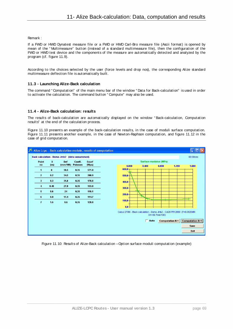
11- Alize Back-calculation: Data, computation and results
ALIZE-LCPC Routes - User manual version 1.3 page 69
Remark :
If a FWD or HWD Dynatest measure file or a FWD or HWD Carl-Bro measure file (Ascii format) is opened by mean of the “Multimeasure” button (instead of a standard multimeasure file), then the configuration of the FWD or HWD test device and the components of the measure are automatically detected and analyzed by the program (cf. figure 11.9).
According to the choices selected by the user (force levels and drop nos), the corresponding Alize standard multimeasure deflection file is automatically built.
11.3 - Launching Alize-Back calculation
The command “Computation” of the main menu bar of the window “Data for Back-calculation” is used in order to activate the calculation. The command button “Compute” may also be used.
11.4 - Alize-Back calculation: results
The results of back-calculation are automatically displayed on the window “Back-calculation, Computation results” at the end of the calculation process. Figure 11.10 presents an example of the back-calculation results, in the case of moduli surface computation. Figure 11.11 presents another example, in the case of Newton-Raphson computation, and figure 11.12 in the case of grid computation.
Figure 11.10: Results of Alize-Back calculation – Option surface moduli computation (example)
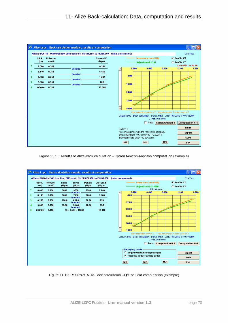
11- Alize Back-calculation: Data, computation and results
ALIZE-LCPC Routes - User manual version 1.3 page 70
Figure 11.11: Results of Alize-Back calculation – Option Newton-Raphson computation (example)
Figure 11.12: Results of Alize-Back calculation – Option Grid computation (example)
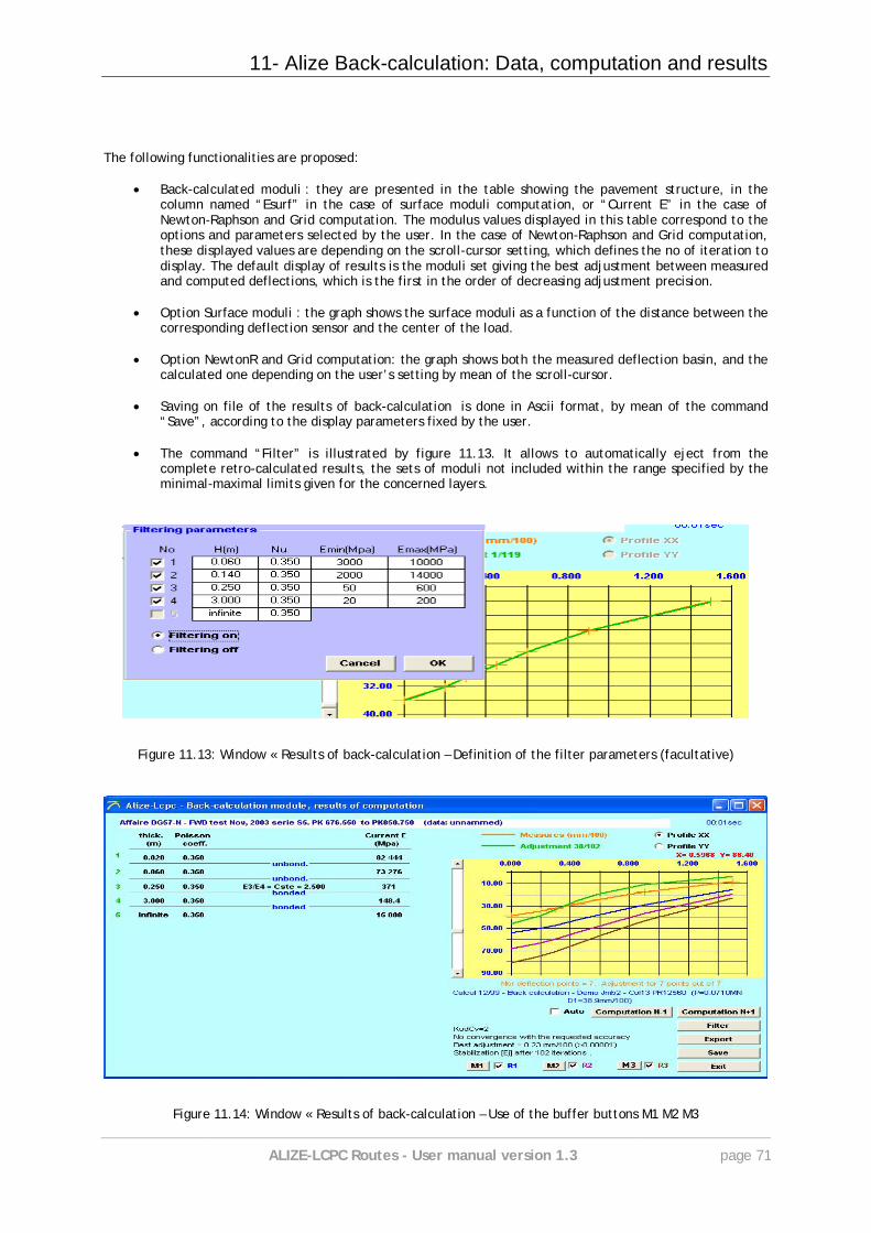
11- Alize Back-calculation: Data, computation and results
ALIZE-LCPC Routes - User manual version 1.3 page 71
The following functionalities are proposed:
Back-calculated moduli : they are presented in the table showing the pavement structure, in the column named “Esurf” in the case of surface moduli computation, or “Current E” in the case of Newton-Raphson and Grid computation. The modulus values displayed in this table correspond to the options and parameters selected by the user. In the case of Newton-Raphson and Grid computation, these displayed values are depending on the scroll-cursor setting, which defines the no of iteration to display. The default display of results is the moduli set giving the best adjustment between measured and computed deflections, which is the first in the order of decreasing adjustment precision.
Option Surface moduli : the graph shows the surface moduli as a function of the distance between the
corresponding deflection sensor and the center of the load.
Option NewtonR and Grid computation: the graph shows both the measured deflection basin, and the calculated one depending on the user’s setting by mean of the scroll-cursor.
Saving on file of the results of back-calculation is done in Ascii format, by mean of the command
“Save”, according to the display parameters fixed by the user.
The command “Filter” is illustrated by figure 11.13. It allows to automatically eject from the complete retro-calculated results, the sets of moduli not included within the range specified by the minimal-maximal limits given for the concerned layers.
Figure 11.13: Window « Results of back-calculation – Definition of the filter parameters (facultative)
Figure 11.14: Window « Results of back-calculation – Use of the buffer buttons M1 M2 M3

11- Alize Back-calculation: Data, computation and results
ALIZE-LCPC Routes - User manual version 1.3 page 72
The role of the buffer buttons M1, M2 and M3 is illustrated by figure 11 .14. Clicking the button Mj launches the storage of the selected deflection profile (computed) in the internal buffer Bj. Then ticking the tick-box Rj displays the drawing of the memorized basin on the graph. This function may be useful in order to directly evaluate the effect of variable computation hypothesis – as layer thicknesses, interface conditions, fixed modulus values … - on the results of the back-calculation.

Appendix A1: The rational pavement design approach
ALIZE-LCPC Routes - User manual version 1.3 page 73
12. Appendix A1: The rational pavement design approach
A1.1 - General framework of rational pavement design
The primary purpose of the rational method is to oversee the design operations of new road and highway pavements, for all categories of traffic (running the gamut from low-traffic pavements to high-traffic pavements). Within this application context, the design approach, the set of associated hypotheses and the tools to be implemented have been fully laid out. Moreover, the general rational design approach has been the focus of a variety of transpositions, aimed at its adaptation to other types of design: differing traffic loads (e.g. industrial carriers, airport loads), other design problem areas (e.g. reinforcement of damaged pavements). The Alize software program is also applicable to these specific uses, without its implementation conditions being necessarily, in this case, entirely contained within an official method. In any event, this software facilitates the practical running of numerical computations required for designing pavement structures. The design of pavement structures extends far beyond these numerical aspects and still lies within the domain of pavement mechanics specialists, whose expertise cannot be replaced despite the level of effectiveness this software is able to offer.
A2.2 - General approach to rational pavement design
Within the scope of common use, the rational design approach encompasses the three following primary phases:
2.1 - The choice of type of structure and component materials
This choice depends upon the framework and specificities of the project under examination. The pavement structure may be of the flexible type, the thick bituminous type, semi-rigid, rigid, mixed or inverse. Each type of structure is associated with the possible use of materials, themselves divided into five families: hydrocarbon materials, materials treated with hydraulic binders, concretes, untreated materials, and soils.

Appendix A1: The rational pavement design approach
ALIZE-LCPC Routes - User manual version 1.3 page 74
2.2 - Determination of allowable stresses within the various materials:
The computation of allowable stresses within the various materials composing the pavement structure stems from two damage models on which the rational method has been based:
2.2.1 - for treated materials (hydrocarbon, treated with hydraulic binders, and concretes): The model adopted is that of fatigue-induced damage submitted to repeated tensile stresses as a result of bending exerted by traffic (the Wöhler model). The allowable stress is then a decreasing function of the number of loadings applied by the traffic and may be expressed in the following general form:
Stadm = AxPxNb
where: A and b = descriptive parameters of the material's fatigue behavior, as generated from
fatigue tests on laboratory specimens (b < 0); P = additional coefficients for incorporating various factors, which have not been
reproduced by raw results from the laboratory fatigue tests; N = number of rolling load cycles (i.e. cumulative traffic) over the entire service
life cycle ascribed to the pavement.
2.2.2 - for untreated materials (untreated gravels and soils): The model adopted is that of damage caused by the accumulation of irreversible plastic strains (rutting), as generated from the vertical compressive stresses exerted by the traffic. The expression of allowable vertical compressive stresses does not stem directly from laboratory tests, but rather from more empirical considerations:
Szadm = AxNb
where: A and b = parameters of an empirical origin, independent of the specific untreated
material being examined, yet in practice varying as a function of both the type of pavement and the intensity of traffic (new vs. reinforced pavement, light vs. heavy traffic, etc.).
N = number of rolling load cycles – same as for Section 2.2.1 above.

Appendix A1: The rational pavement design approach
ALIZE-LCPC Routes - User manual version 1.3 page 75
2.3 - Determination of the thickness of the various material layers:
The stresses created by rolling loads within the various material layers are calculated using the Burmister linear elastic multilayer model (see Section 3.1), with Smaxj designating the highest stress from the standpoint of the damage criteria defined above and with support provided by material layer n°j. The thickness determination of each material layer then relies upon verifying the non-breaking criterion of the material under investigation throughout the pavement service life, i.e.:
Smaxj ≤ Sadmj
where: Smaxj: maximum stress generated by the traffic within material layer n°j, as stipulated by
the damage mode associated with the type of material being considered (bending-induced horizontal tension or vertical compression, see Section 2.2);
Sadmj: stress allowed by the specific material (see Section 2.2).
The ultimate determination of thicknesses Hj of the various layers of materials constituting the pavement structure does not, in general, lead to a direct solution (absence of explicit solution {Hj = f(N)}). In most cases, this determination is performed by means of an inverse iterative approach, as diagrammed in Figure A1 below. The numerical solution to the problem presented is moreover not at all unique. The final choice also depends on both technological considerations (e.g. minimum and maximum layer thicknesses as a function of the material, traffic classification, etc.) and empirical considerations (e.g. thickness of the surface layers).
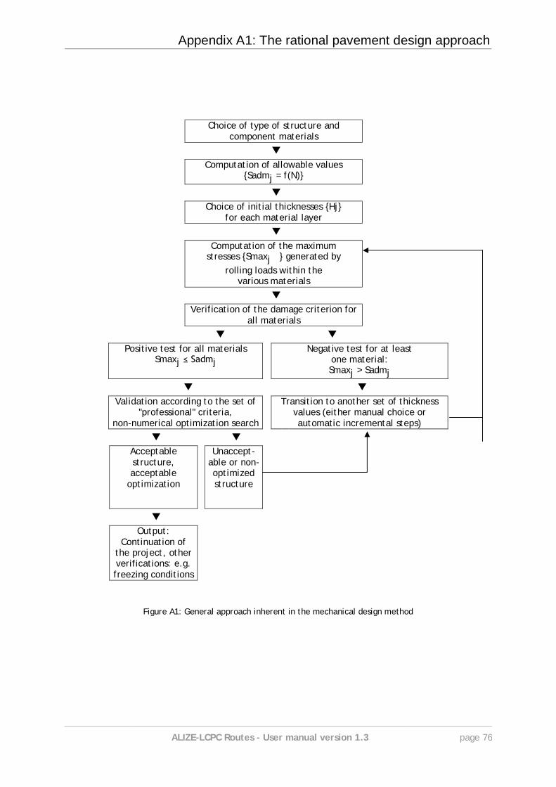
Appendix A1: The rational pavement design approach
ALIZE-LCPC Routes - User manual version 1.3 page 76
Choice of type of structure and component materials
▼
Computation of allowable values {Sadmj = f(N)}
▼ Choice of initial thicknesses {Hj}
for each material layer ▼
Computation of the maximum stresses {Smaxj } generated by
rolling loads within the various materials
▼ Verification of the damage criterion for
all materials ▼ ▼
Positive test for all materials Smaxj ≤ Sadmj
Negative test for at least one material: Smaxj > Sadmj
▼ ▼
Validation according to the set of "professional" criteria,
non-numerical optimization search
Transition to another set of thickness values (either manual choice or automatic incremental steps)
▼ ▼
Acceptable structure, acceptable
optimization
Unaccept-able or non-optimized structure
▼
Output: Continuation of
the project, other verifications: e.g. freezing conditions
Figure A1: General approach inherent in the mechanical design method

Appendix A1: The rational pavement design approach
ALIZE-LCPC Routes - User manual version 1.3 page 77
A3.3 - The mechanical computation model
The computation engine enables determining the stresses generated by traffic within the various layers of materials composing the pavement core by making use of the Burmister model. This model relies upon a mechanical description of the structure using a semi-infinite foundation, generated by superimposing constant thickness material layers, featuring isotropic linear elastic behavior. The number of descriptive parameters for the mechanical behavior of each material can thus be reduced to two: strain modulus E, and Poisson's ratio . Each interface between adjacent layers may be set as bonded, sliding or semi-bonded. The loading applied by rolling loads at the pavement surface is represented by a set of circular disks, each loaded by a static and uniform vertical pressure. Any combination of circular elementary loads of this type is indeed possible, a feature that enables reproducing the profiles of axles, bogie units, a vehicle or of the widest array of vehicles. Within more commonplace design operations, a unique loading, designated as the reference loading, is typically applied at the model surface; this reference loading is specific to the context in which the rational design method is being applied. For example, a 65-kN twinning (3.25 kN per wheel, with a 6.62 MPa contact pressure) constitutes, except in special cases, the reference design load for pavement structures on France's road and highway networks. In some airport pavement design applications, the reference load will be taken as the isolated 30-kN wheel load, etc.
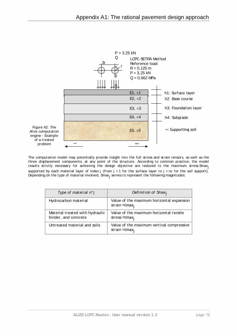
Appendix A1: The rational pavement design approach
ALIZE-LCPC Routes - User manual version 1.3 page 78
P = 3.25 kN Q = 0.662 MPa
Figure A2: The Alize computation engine - Example
of a treated problem
The computation model may potentially provide insight into the full stress and strain tensors, as well as the three displacement components, at any point of the structure. According to common practice, the model results strictly necessary for achieving the design objective are reduced to the maximum stress Smaxj supported by each material layer of index j (from j = 1 for the surface layer to j = nc for the soil support). Depending on the type of material involved, Smaxj serves to represent the following magnitudes:
Type of material n°j Definition of Smaxj
Hydrocarbon material
Value of the maximum horizontal expansion strain tmaxj
Material treated with hydraulic binder, and concrete
Value of the maximum horizontal tensile stress tmaxj
Untreated material and soils Value of the maximum vertical compressive strain tmaxj
h2: Base course
h3: Foundation layer
h4: Subgrade
∞: Supporting soil
h1: Surface layer
+∞ -∞
3r r
LCPC-SETRA Method Reference load: R = 0,125 m P = 3,25 kN Q = 0,662 MPa
E1, 1 E2, 2
E3, 3
E4, 4
E5, 5
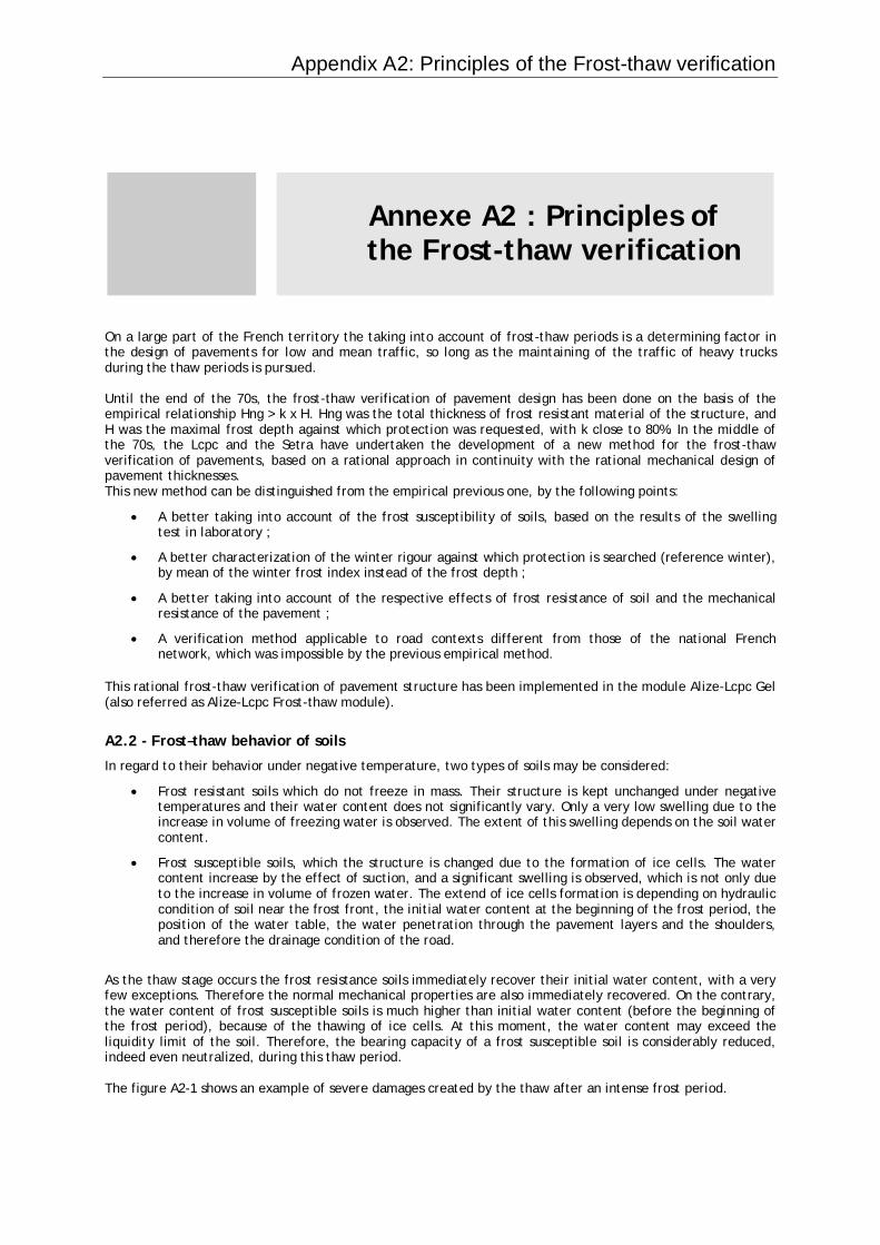
Appendix A2: Principles of the Frost-thaw verification
13. Annexe A2 : Principles of the Frost-thaw verification
On a large part of the French territory the taking into account of frost-thaw periods is a determining factor in the design of pavements for low and mean traffic, so long as the maintaining of the traffic of heavy trucks during the thaw periods is pursued. Until the end of the 70s, the frost-thaw verification of pavement design has been done on the basis of the empirical relationship Hng > k x H. Hng was the total thickness of frost resistant material of the structure, and H was the maximal frost depth against which protection was requested, with k close to 80%. In the middle of the 70s, the Lcpc and the Setra have undertaken the development of a new method for the frost-thaw verification of pavements, based on a rational approach in continuity with the rational mechanical design of pavement thicknesses. This new method can be distinguished from the empirical previous one, by the following points:
A better taking into account of the frost susceptibility of soils, based on the results of the swelling test in laboratory ;
A better characterization of the winter rigour against which protection is searched (reference winter), by mean of the winter frost index instead of the frost depth ;
A better taking into account of the respective effects of frost resistance of soil and the mechanical resistance of the pavement ;
A verification method applicable to road contexts different from those of the national French network, which was impossible by the previous empirical method.
This rational frost-thaw verification of pavement structure has been implemented in the module Alize-Lcpc Gel (also referred as Alize-Lcpc Frost-thaw module).
A2.2 - Frost–thaw behavior of soils
In regard to their behavior under negative temperature, two types of soils may be considered:
Frost resistant soils which do not freeze in mass. Their structure is kept unchanged under negative temperatures and their water content does not significantly vary. Only a very low swelling due to the increase in volume of freezing water is observed. The extent of this swelling depends on the soil water content.
Frost susceptible soils, which the structure is changed due to the formation of ice cells. The water content increase by the effect of suction, and a significant swelling is observed, which is not only due to the increase in volume of frozen water. The extend of ice cells formation is depending on hydraulic condition of soil near the frost front, the initial water content at the beginning of the frost period, the position of the water table, the water penetration through the pavement layers and the shoulders, and therefore the drainage condition of the road.
As the thaw stage occurs the frost resistance soils immediately recover their initial water content, with a very few exceptions. Therefore the normal mechanical properties are also immediately recovered. On the contrary, the water content of frost susceptible soils is much higher than initial water content (before the beginning of the frost period), because of the thawing of ice cells. At this moment, the water content may exceed the liquidity limit of the soil. Therefore, the bearing capacity of a frost susceptible soil is considerably reduced, indeed even neutralized, during this thaw period. The figure A2-1 shows an example of severe damages created by the thaw after an intense frost period.
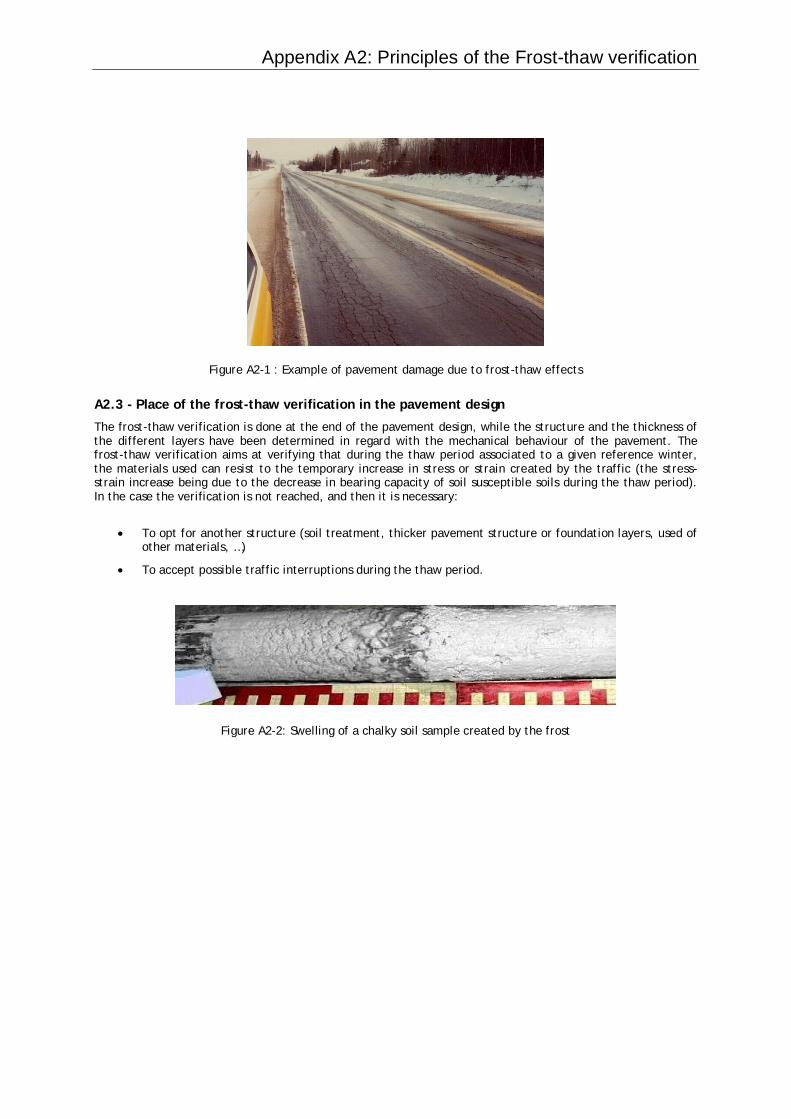
Appendix A2: Principles of the Frost-thaw verification
Figure A2-1 : Example of pavement damage due to frost-thaw effects
A2.3 - Place of the frost-thaw verification in the pavement design
The frost-thaw verification is done at the end of the pavement design, while the structure and the thickness of the different layers have been determined in regard with the mechanical behaviour of the pavement. The frost-thaw verification aims at verifying that during the thaw period associated to a given reference winter, the materials used can resist to the temporary increase in stress or strain created by the traffic (the stress-strain increase being due to the decrease in bearing capacity of soil susceptible soils during the thaw period). In the case the verification is not reached, and then it is necessary:
To opt for another structure (soil treatment, thicker pavement structure or foundation layers, used of other materials, …)
To accept possible traffic interruptions during the thaw period.
Figure A2-2: Swelling of a chalky soil sample created by the frost

Appendix A2: Principles of the Frost-thaw verification
A2.4 - Definitions and notations
Frost index : The atmospheric frost index is the cumulated sum of the mean daily temperatures of the air under shelter, calculated from the first day having a negative mean temperature. The frost indexes are expressed in absolute value, in the units °Cxday. The following frost indexes are used: - Iatm : atmospheric frost index ; - Is : pavement surface frost index ; - It : frost index transmitted at the bottom of the pavement structure. Frost Quantity : It is the square root of the frost index (unity [°C.day]1/2). The following frost quantities are used: - Qatm atmospheric frost quantity; - Qs pavement surface frost quantity; - Qt (or Qpf) : frost quantity transmitted at the bottom of the pavement structure.
A2.5 - General organization of the frost-thaw verification
Only the pavements lying on frost susceptible materials have to be verified against the frost-thaw effects. The figure A2-3 represents the general progress of frost-thaw verification studies. The verification of the frost-thaw behaviour involves comparing:
the atmospheric frost index chosen as reference, IR, that characterizes the severity of winter against which it has been chosen to protect the pavement,
and the atmospheric frost index that the pavement is able to withstand, which is called the allowed frost index IA. This index is evaluated according to the frost susceptibility of the subgrade, the thermal protection and mechanical function fulfilled by the pavement.
The pavement structure is designed so that the allowed frost index IA of the pavement is higher than the reference frost index IR. If the frost index happens to be larger than IA, the structure has to be modified (other higher thicknesses, or materials, or pavement foundation …), or thaw barriers may have to be installed to protect the pavement during thaw periods. Choice of the reference winter : The winter chosen as the reference (and therefore the reference atmospheric frost index) depends on road manager policy. This choice will affect the frequency with which thaw barriers are installed, and therefore the frequency with which traffic is interrupted. On the French national network, two characteristics reference winter may be generally considered (cf. The French Catalogue for new pavement structures, 1998) :
the exceptional winter, which is the most severe winter encountered on the period 1951-1997,
or the rigorous not exceptional winter, which is the decennial winter on the same period. The 1998 Catalogue also indicates the frost indexes of the exceptional winter and the rigorous not exceptional winters recorded by the main meteorological stations on the 1951-1997 period.
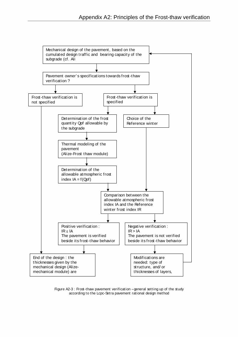
Appendix A2: Principles of the Frost-thaw verification
Figure A2-3 : Frost-thaw pavement verification – general setting up of the study
according to the Lcpc-Setra pavement rational design method
Mechanical design of the pavement, based on the cumulated design traffic and bearing capacity of the subgrade (cf. Ali
Logiciel Frost-thaw verification is specified
Thermal modeling of the pavement (Alize-Frost thaw module)
Determination of the allowable atmospheric frost index IA = f(Qpf)
Comparison between the allowable atmospheric frost index IA and the Reference winter frost index IR
End of the design : the thicknesses given by the mechanical design (Alize-mechanical module) are adopted
Negative verification : IR > IA The pavement is not verified beside its frost-thaw behavior
Pavement owner’s specifications towards frost-thaw verification ?
Frost-thaw verification is not specified
Choice of the Reference winter
Determination of the frost quantity Qpf allowable by the subgrade
Positive verification : IR ≤ IA The pavement is verified beside its frost-thaw behavior
Modifications are needed: type of structure, and/or thicknesses of layers, and/or capping layer …
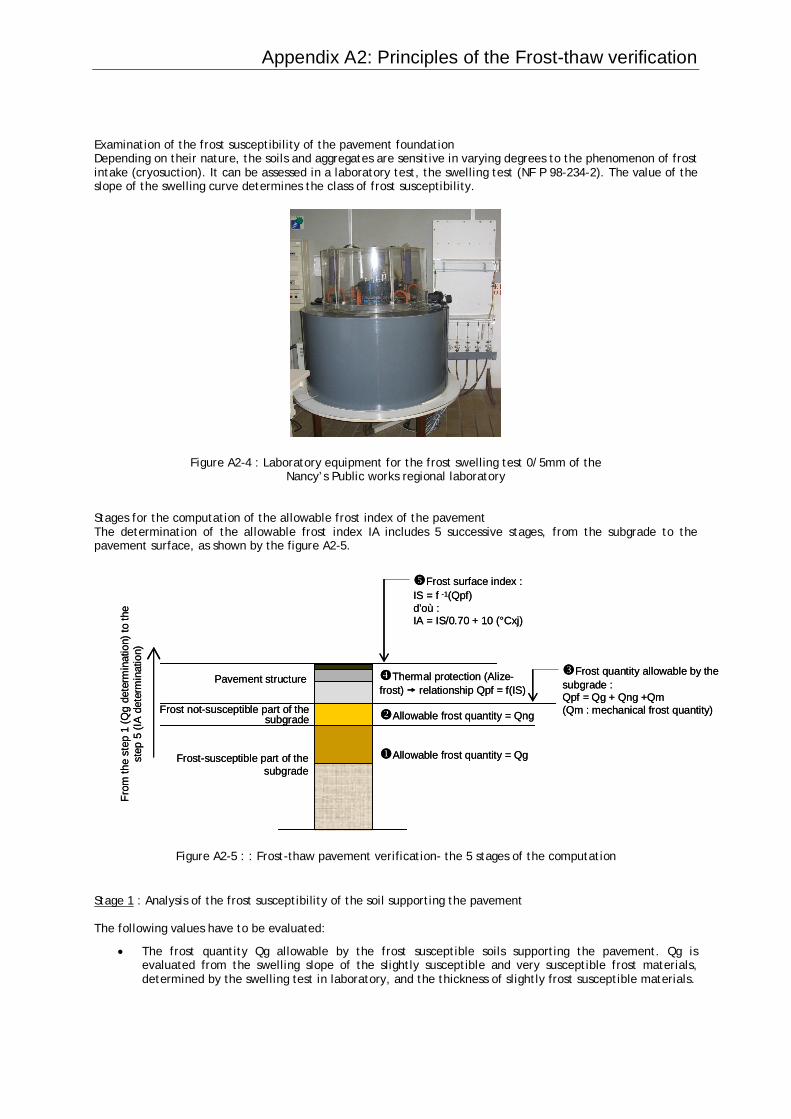
Appendix A2: Principles of the Frost-thaw verification
Examination of the frost susceptibility of the pavement foundation Depending on their nature, the soils and aggregates are sensitive in varying degrees to the phenomenon of frost intake (cryosuction). It can be assessed in a laboratory test, the swelling test (NF P 98-234-2). The value of the slope of the swelling curve determines the class of frost susceptibility.
Figure A2-4 : Laboratory equipment for the frost swelling test 0/5mm of the Nancy’s Public works regional laboratory
Stages for the computation of the allowable frost index of the pavement The determination of the allowable frost index IA includes 5 successive stages, from the subgrade to the pavement surface, as shown by the figure A2-5.
Frost-susceptible part of the subgrade
Frost not-susceptible part of the subgrade
Allowable frost quantity = Qg
Allowable frost quantity = Qng
Frost quantity allowable by the subgrade :Qpf = Qg + Qng +Qm(Qm : mechanical frost quantity)
Pavement structure Thermal protection (Alize-frost) relationship Qpf = f(IS)
Frost surface index : IS = f -1(Qpf)d’où : IA = IS/0.70 + 10 (°Cxj)
From
the
step
1 (Q
gde
term
inat
ion)
to th
e st
ep 5
(IA
dete
rmin
atio
n)
Figure A2-5 : : Frost-thaw pavement verification- the 5 stages of the computation Stage 1 : Analysis of the frost susceptibility of the soil supporting the pavement The following values have to be evaluated:
The frost quantity Qg allowable by the frost susceptible soils supporting the pavement. Qg is evaluated from the swelling slope of the slightly susceptible and very susceptible frost materials, determined by the swelling test in laboratory, and the thickness of slightly frost susceptible materials.
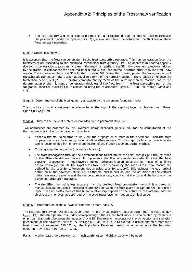
Appendix A2: Principles of the Frost-thaw verification
The frost quantity Qng, which represents the thermal protection due to the frost resistant materials of the pavement foundation layer and soil. Qng is evaluated from the nature and the thickness of these frost resistant materials.
Step 2 : Mechanical analysis It is accepted that the frost can penetrate into the frost-susceptible subgrade. This frost penetration (over the thickness e) corresponding to the additional mechanical frost quantity Qm. The decrease in bearing capacity due to this penetration creates an increase in the maximal tensile stress S2 in the pavement structure induced by the traffic, in comparison with the maximal stress S1 over the normal situation other than the frost-thaw season. The increase of the stress S2 is limited to about 5%. During the thawing phase, the Young modulus of the subgrade subject to thaw is taken as equal to a tenth of the normal modulus in the situation other than the frost/thaw period, ie E(Pf)/10. Iterative computations by mean of the Alize-mechanical module lead to the determination of the thickness e (penetration thickness of the frost front in the frost susceptible part of the subgrade). Then the quantity Qm is calculated using the relationship: Qm= e/10 (unities: sqare(°C.day) and cm). Stage 3 : Determination of the frost quantity allowable by the pavement foundation layer The quantity of frost considered as allowable at the top of the capping layer is obtained as follows: Qpf = Qg + Qng +Qm Stage 4 : Study of the thermal protection provided by the pavement structure Two approaches are proposed by the Pavement design technical guide (1994) for the computation of the thermal protection due to the pavement structure:
either a thermal calculation to work out the propagation of frost in the pavement. Then the frost propagation is calculated using the Alize – Frost-thaw module. This first approach is the more accurate and is recommended in the normal application of the French pavement design method.
Or using simplified equation (manual application).
The frost propagation through the pavement leads to determine the relationship Qpf = f(IS) by mean of the Alize – Frost-thaw module. It implements the Fourier’s model in order to solve the heat equation propagation in multilayered mixed unfrosted-frosted structure by mean of a finite differences algorithm. All the hypotheses taken into account by the Alize – Frost-thaw module are defined by the Lcpc-Setra Pavement design guide Lcpc-Setra (1994). This includes the geometrical definition of the pavement structure, its thermal characteristics, and the definition of the vertical initial temperature profile and the temperature boundary condition at the top and the bottom of the pavement structure + subgrade.
The simplified method is less accurate than the previous frost propagation method. It is based on manual calculation using a linearized relationship between the frost quantities Qpf and Qs. For a given layer, the two coefficients of this linear relationship depend on the nature of the material and the thickness of the layer, as described by the Lcpc-Setra Pavement design technical guide.
Stage 5 : Determination of the allowable atmospheric frost index IA The relationship between Qpf and IS established in the previous stage 4 leads to determine the value of IS = finverse(Qpf). The atmospheric frost index corresponding to the surface frost index IS is calculated by mean of a empirical relationship between the indexes IA and IS. This relation accounts for the convection and radiation phenomena at the pavement surface. At average altitude, with little to average sunshine and an atmospheric frost index not exceeding 210 °C.day, the Lcpc-Setra Pavement design guide recommends the following equation: IA = IS/0.7 + 10 (unity: °C.day). For all the other cases (very severe frost, much sunshine) an individual study will be need.