Alternating oscillatory and stochastic dynamics in a model for a neuronal assembly

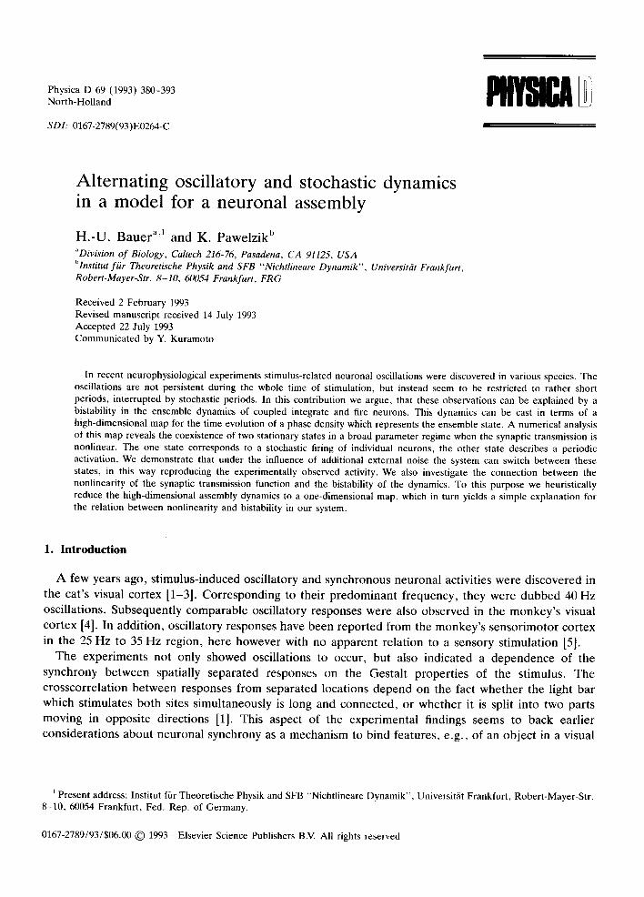
Physica D 69 (1993) 380-393 North-Holland

SDI: 0167-2789(93)E0264-C

Alternating oscillatory and stochastic dynamics in a model for a neuronal assembly

H . - U . B a u e r a'l and K. Pawelz ik b

aDivision of Biology, Caltech 216-76, Pasadena, CA 91125, USA blnstitut fiir Theoretische Physik and SFB "Nichtlineare Dynamik", Universitdt Frankfurt, Robert-Mayer-Str. 8-10, 60054 Frankfurt, FRG

Received 2 February 1993 Revised manuscript received 14 July 1993 Accepted 22 July 1993 Communicated by Y. Kuramoto

In recent neurophysiological experiments stimulus-related neuronal oscillations were discovered in various species. The oscillations are not persistent during the whole time of stimulation, but instead seem to be restricted to rather short periods, interrupted by stochastic periods. In this contribution we argue, that these observations can be explained by a bistability in the ensemble dynamics of coupled integrate and fire neurons. This dynamics can be cast in terms of a high-dimensional map for the time evolution of a phase density which represents the ensemble state. A numerical analysis of this map reveals the coexistence of two stationary states in a broad parameter regime when the synaptic transmission is nonlinear. The one state corresponds to a stochastic firing of individual neurons, the other state describes a periodic activation. We demonstrate that under the influence of additional external noise the system can switch between these states, in this way reproducing the experimentally observed activity. We also investigate the connection between the nonlinearity of the synaptic transmission function and the bistability of the dynamics. To this purpose we heuristically reduce the high-dimensional assembly dynamics to a one-dimensional map, which in turn yields a simple explanation for the relation between nonlinearity and bistability in our system.

I. Introduction

A few years ago, stimulus-induced oscillatory and synchronous neuronal activities were discovered in the cat's visual cortex [1-3]. Corresponding to their predominant frequency, they were dubbed 40 Hz oscillations. Subsequently comparable oscillatory responses were also observed in the monkey's visual cortex [4]. In addition, oscillatory responses have been reported from the monkey's sensorimotor cortex in the 25 Hz to 35 Hz region, here however with no apparent relation to a sensory stimulation [5].

The experiments not only showed oscillations to occur, but also indicated a dependence of the synchrony between spatially separated responses on the Gestalt properties of the stimulus. The crosscorrelation between responses from separated locations depend on the fact whether the light bar which stimulates both sites simultaneously is long and connected, or whether it is split into two parts moving in opposite directions [1]. This aspect of the experimental findings seems to back earlier considerations about neuronal synchrony as a mechanism to bind features, e.g., of an object in a visual

Present address: Institut f/Jr Theoretische Physik and SFB "Nichtlineare Dynamik", Universit~it Frankfurt, Robert-Mayer-Str . 8-10, 60054 Frankfurt, Fed. Rep. of Germany.

0167-2789/93/$06.00 © 1993 - Elsevier Science Publishers B.V. All rights reserved

H.-U. Bauer, K. Pawelzik / Alternating dynamics in a neuronal assembly 381

scene [6,7]. The experiments gave rise to a large number of theoretical contributions, which were primarily concerned with the establishment of synchrony in layers of coupled oscillators [8-12].

The ansatz of simple limit cycle oscillators for the dynamics of a local neuron group however, is questionable when considering the detailed time structure of the measured responses. An analysis of the responses from cat visual cortex with methods based on correlation functions revealed a huge amount of variability, both in the occurrence of oscillatory episodes as well as in the amount of synchrony between neurons at a considerable cortical distance [13,14]. Analysis of the time resolved predictability of local field potential data showed that the oscillatory responses occur only during rather short periods, which are interrupted by stochastic periods [15]. In a recent contribution describing oscillations in the monkey sensorimotor cortex, the switching between oscillatory and stochastic periods in the data is easy to identify [5]. The length distribution of the oscillatory periods was roughly estimated to be exponential, compatible with a Poisson process switching between the two states.

These observations suggest that the dynamics of the underlying system is more complex than a limit cycle emerging from a Hopf bifurcation. In the present work we derive and analyze a model of a local neuronal pool, which captures this alternating dynamics. While at first sight this might seem to imply a complex model which includes many contingent details we will show that it is sufficient to include the spiking nature of neurons together with the nonlinear synaptic efficacies in order to obtain a bistabil assembly dynamics. Under the influence of external noise the system then can switch and reproduce interesting aspects of the phenomena. In a model of oscillators with point-like coupling, which resembles a real neuronal system to a higher degree than models with permanent coupling, bistability has already been described [16]. However, the fixed point there corresponds to silent neurons. This is in contrast to the observation, that the mean firing rate is not much affected by the apparent switching between the two states in the cat data.

In the second section we show that the model for the assembly dynamics can be brought into a simple mathematical form which for discrete neuron states is a high-dimensional map acting on a phase density, which represents the state of the assembly.

The dynamics of this phase distribution is numerically analyzed in the third section, revealing that a nonlinear synaptic transmission function can induce a bistability of the phase dynamics. We then proceed in the fourth section to investigate a possible switching between these states under the influence of external noise. The resulting overall dynamics is then compared to the experimental findings. In a fifth section we further investigate the relation between the nonlinearity of the synaptic transmission function, and the occurence of a bistability in the dynamics. Finally a discussion of the results, and their possible functional consequences concludes the paper.

2. Dynamics of the assembly phase density

In this chapter we derive a description for the dynamics of an externally driven, self-excitatory neuronal assembly in the form of a rather simple map. To this purpose we first sketch a few general arguments about single neuron elements, and a suitable assembly averaging. These arguments are then connected to yield the desired assembly dynamics in discretized form.

First we assume, that the excitability PI of a single neuron is related to its input I and its threshold O by a sigmoidal function,

Pio: s igm(/ - 0 ) . (2.1)

382 H.-U. Bauer, K. Pawelzik / Alternating dynamics in a neuronal assembly

Pj. has the interpretation of a transition probability for eliciting a spike within a time interval d ~1. The function sigm compares the input of a neuron to its threshold using a softened step-function, in this way reflecting the intrinsic stochasticity of the neuron. Following a common choice in the neural network literature [17] we take

sigm(x) = 1 / (1+ e x). (2.2)

In the next step, we assume, that the state of the neuron at time t depends only on the time 4, = t - t' elapsed since the last spike at time t ' . In other words we assume that the neuron has no memory which goes back beyond the last spike. This assumption can very easily be modeled by having a firing threshold O(~b), which depends only on the absolute and relative refractory periods of the neuron:

{~ if ~b < trefr , (2.3) 0 ( 6 ) = O0 + O 1 e [ - - ( ~ / T r e f r ) ] i f ~ >/refr •

In this way the neuron spike dynamics is modeled by a renewal process, a framework which has a long tradition in the analysis of spike trains [18]. Modeling neuronal spike dynamics in terms of excitability functions has recently been discussed by Gerstner and Van Hemmen [19], who show, among other things, the adequacy of this approach to reproduce the spiking behaviour of the Hodgkin-Huxley model [20]. In this view, the process dominating the repetitive firing dynamics of neurons is the recovery of spike-generating membrane channels (sodium and potassium channels), which proceeds independently of external input. The external input controls the firing probability of the neuron, once it recovered. Reflecting the property of neurons to be coincidence detectors, the external input is not integrated in this approach.

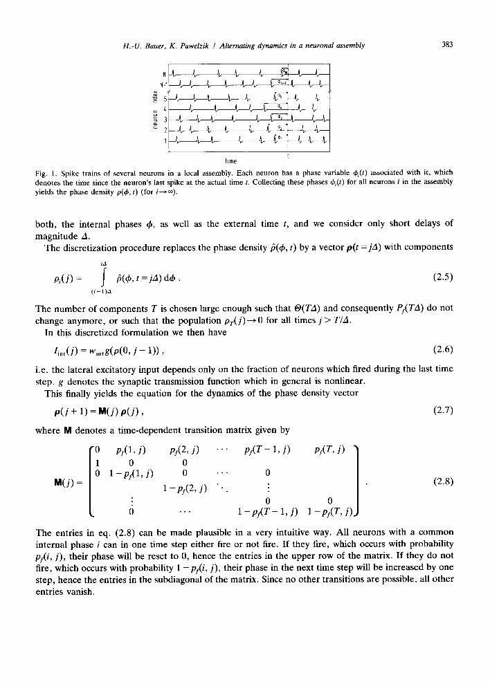
We now consider an ensemble of such neurons, which all receive external input from the same stimulus (in other words which form an assembly of neurons). We assume the number of neurons to be large and describe the state of the assembly by the probability density tS(~b, t) where ~(~b, t) d~b gives the probability to find a neuron with 4, E [~b, ~b + d~b] at time t. An intuitive picture of such an ensemble, the internal phases ~bi, and the phase distribution ~ is given in fig. 1.

The input to a single neuron in the assembly will consist of two parts,

I = t e x t q- l in t . ( 2 . 4 )

The first term, Iext, describes the input due to the external stimulation, and is assumed to be uniform for all neurons in the assembly. The second term l in t describes the input due to lateral excitatory connections within the assembly. Only neurons which just fired can contribute to this lateral excitation. However, since the transmission of a spike is not instantaneous, we have to take time delays into account. All their effects can in principle be included into a kernel which is useful for deriving a continuous assembly dynamics analogous to the model discussed in [19].

Here, however, we consider this dynamics only in discretized form with a discretization step of za for

,1 Pr can be derived from a rate r which is independent from the discretization A via ~+gt

PM,)= l -exp[ f r(~h')d6'].

This relation is useful for rescaling of the excitability when the discretization is changed. For A and A' small and r smooth we approximately have

P) = 1 - (1 - PAa'/a.


N-~ L L N-I ~ /~

4 L L

2 ~ L

time

I

¢--¢

I

Fig. 1. Spike trains of several neurons in a local assembly. Each neuron has a phase variable ~bi(t ) associated with it, which denotes the t ime since the neuron 's last spike at the actual time t. Collecting these phases ~bi(t ) for all neurons i in the assembly yields the phase density p(qb, t) (for i---~ oo).

both, the internal phases 4), as well as the external time t, and we consider only short delays of magnitude A.

The discretization procedure replaces the phase density/~(~b, t) by a vector p(t = jza) with components

iA

pi(j) = J t)(th, t =jA) dtb. (2.5) ( i -1 )a

The number of components T is chosen large enough such that @(TA) and consequently Pi(Tza) do not change anymore, or such that the population pr(j)---~O for all times j > T/zl.

In this discretized formulation we then have

lint(J) = Wintg(p(O , j -- 1)), (2.6)

i.e. the lateral excitatory input depends only on the fraction of neurons which fired during the last time step. g denotes the synaptic transmission function which in general is nonlinear.

This finally yields the equation for the dynamics of the phase density vector

p ( j + 1) = M(j) p ( j ) , (2.7)

where M denotes a t ime-dependent transition matrix given by

"0 py(1, j ) ,o,(2, j ) - . . pI(T- 1, j) pr(T, j) 1 0 0 0 1 - p l ( 1 , j ) 0 . . - 0

1 - p c ( 2 , j) "- • 0 0

0 "" 1 - p t ( T - 1, j ) 1 - p i ( T , j)

M(j) = (2.8)

The entries in eq. (2.8) can be made plausible in a very intuitive way. All neurons with a common internal phase i can in one time step either fire or not fire. If they fire, which occurs with probability pi(i, j) , their phase will be reset to 0, hence the entries in the upper row of the matrix. If they do not fire, which occurs with probability 1 -p i ( i , j ) , their phase in the next time step will be increased by one step, hence the entries in the subdiagonal of the matrix• Since no other transitions are possible, all other entries vanish.


The firing probabilities pf(i, j) entering eq. (2.8) are the firing probabilities of eq. (2.1), which read in discretized formulation, using eqs. (2 .2)-(2 .4) , and (2.6),

1 PsU,' J) - 1 + exp[lex t + w,,tg(p,,(j)) - 6~(i)]

I (2.9)

Eqs. (2 .7)- (2 .9) now describe the phase distribution dynamics in terms of a (T + 1)-dimensional map. The map is highly nonlinear since p does not only directly enter the iteration eq. (2.7), but also the transition matrix (2.8) via eq. (2.9).

3. Stationary states of the assembly dynamics

We now investigate the dynamics of this system. The system is nonlinear and high-dimensional which means that analytical results can be expected for special cases only. Therefore we resort to a numerical t reatment. Iteration of the map (2.7) reveals that most initializations p(0) settle into one of two stationary states, depending on the parameters Iext, wint and the synaptic transmission function g.

The one state is a stable fixed point p ( j + 1) = p ( j ) = ft. In this case also the excitability function becomes time independent after transients have died out, i.e. py(i, j) = fij,.

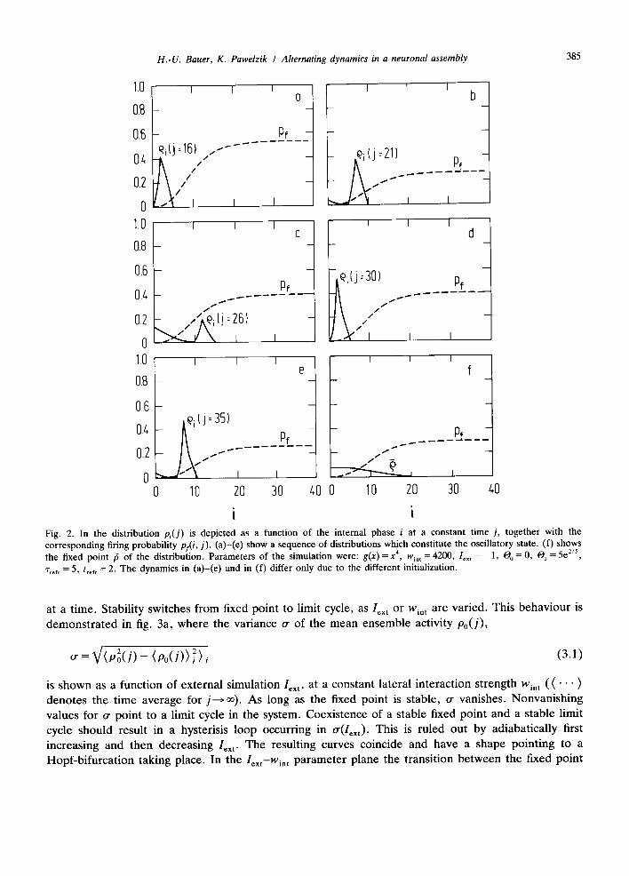
Such a fixed point is depicted in fig. 2f. The initial distribution corresponded to a neuronal assembly where a large fraction of neurons fired in unison at t = 0 (Po(J = 0 ) = 0.6). However , this initial synchronization became lost, and we observed a dispersion effect until finally p became time independent . This fixed point of the dynamics is to be interpreted such that the fraction of neurons firing at each point in time is a constant. The individual neurons, however, fire stochastically, according to their time independent excitability fis" Since in an experimental situation only this stochastic response of individual neurons can be observed, we emphasize this single element property over the constancy of the density and call this state of the system the "stochastic state".

At other parameter values or initializations the system may also exhibit limit cycle dynamics p ( j + To) = p ( j ) , as depicted in figs. 2a-e . Again the system has been initialized with a peak at p0(0). As the system evolves in time, the fraction of neurons around the peak is somewhat diminished, due to the dispersion. However , when a sizeable fraction of the peak neurons fires together again, the firing probability pj. of all the other neurons is increased due to the lateral interaction. Neurons, which had not been part of the peak in the distribution before, are recruited. If this gain is large enough to make up for the dispersion loss, the overall peak amplitude remains unchanged. The system keeps up a periodic firing pattern. We call this state the "periodic state", with many of the neurons taking part in a periodic firing pattern.

In this way our system exhibits both dynamical states which have been observed in the cat cortex: the nonperiodic, stochastic state as well as the periodic state. As has been pointed out in the introduction, the analysis of the physiological data reveals not only the existence of these two states, but also, that they can interchange during one stimulation, in an apparently random fashion. Since one should expect all system parameters to remain constant (apart from noise), this suggests some bistability in the neuronal substrate which carries the oscillations. We therefore proceed to investigate our system with regard to a possible coexistence of both states at one setting of the parameters, depending on the initialization only. To this purpose we varied Iext, wi.t adiabatically with different synaptic transmission functions g.

It turned out that for a linear synaptic transmission function g the system has only one stationary state

H.-U. Bauer, K. Pawelzik Alternating dynamics in a neuronal assembly 385

1.0

0.8

0.6

0.4

0.2

0 1.0

0.8

0.6

/ / / i / /

Pf

I I I C

Pf . 4 ~ . . . . . . . .

/ f

o.2 - ,~ t j :26)

1.0 i e

0.8 -

O.g -

0./-, pf 0.2

0 0 113 213 30 z,O

I I b

I

k I i f

Pf

Pf

Pt_

0 10 20 30 /-,0

i i Fig. 2. In the distribution Pi(J) is depicted as a function of the internal phase i at a constant time j, together with the corresponding firing probabili ty pr(i, j). (a)-(e) show a sequence of distributions which constitute the oscillatory state. (f) shows the fixed point t5 of the distribution. Parameters of the simulation were: g(x)=x 4, w~, t = 4200, l , xt = - 1 , O 0 = 0, @1 = 5e2/5, r, ef, = 5, t,,t, = 2. The dynamics in (a)-(e) and in (f) differ only due to the different initialization.

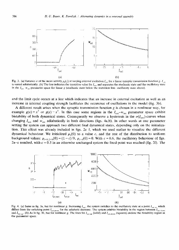
at a time. Stability switches from fixed point to limit cycle, as Iext or wi, t are varied. This behaviour is demonstrated in fig. 3a, where the variance or of the mean ensemble activity Po(J),

o" : ~ / (p2o ( j ) - ( P o ( J ) ) ~) j ( 3 . 1 )

is shown as a function of external simulation Iext, at a constant lateral interaction strength Win t ( ( " ' " ) denotes the time average for j----> oo). As long as the fixed point is stable, o- vanishes. Nonvanishing values for o- point to a limit cycle in the system. Coexistence of a stable fixed point and a stable limit cycle should result in a hysterisis loop occurring in o-(Iext). This is ruled out by adiabatically first increasing and then decreasing I~x t. The resulting curves coincide and have a shape pointing to a Hopf-bifurcation taking place. In the Iext--Wint parameter plane the transition between the fixed point


00z,

OO3

OO2

00;

0 __/

-09 08 Iext

20

15

Winll 0

I E I ~ I

3 -25 2 -15 -1 -05

I ext

(a) (b) Fig. 3. (a) Variance cr of the mean activity p,(j) at varying external excitation l~x , for a linear synaptic transmission function g. 1o,, is varied adiabatically. (b) The line indicates the transition value for lex , and separates the stochastic state and the oscillatory state in the l~x~-W~,,-parameter space for linear g (stochastic state below the transition line, oscillatory state above).

and the l imit cycle occurs at a l ine which indica tes that an increase in ex te rna l exc i t a t ion as well as an

inc rease in in te rna l coupl ing s t rength faci l i ta tes the occurence of osc i l la t ions in the m o d e l (fig. 3b).

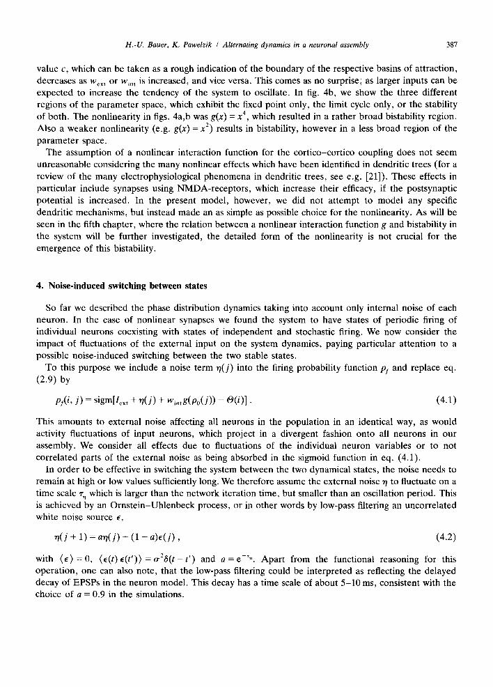
A d i f fe ren t resul t ar ises when the synapt ic t r ansmiss ion funct ion g is chosen in a n o n l i n e a r way, for

e x a m p l e g ( x ) = x 2 o r g ( x ) = x 4. In this case some regions in the Ie×t--Wi, t p a r a m e t e r space exh ib i t

b i s t ab i l i ty of bo th dynamica l s tates . C o n s e q u e n t l y we obse rve a hys teres is in the o-(l~xt)-curves when

chang ing lext and Win t ad iaba t i ca l ly in bo th d i rec t ions (figs. 4a ,b) . In o t h e r words at one p a r a m e t e r

se t t ing the sys tem can a p p r o a c h two d i f ferent final dynamica l s ta tes , d e p e n d i n g only on the ini t ia l iza-

t ion. This effect was a l r e ady inc luded in figs. 2 a - f , which we used ea r l i e r to visual ize the d i f fe ren t

d y n a m i c a l behav iou r . We in i t ia l ized p l (0 ) to a va lue c, and the rest of the d i s t r ibu t ion to un i fo rm

b a c k g r o u n d values : pi=0,2=9(0) = (1 - c ) /9 , pi>9(0) = 0. Wi th c = 0.6, the osc i l l a to ry b e h a v i o u r o f figs.

2 a - e r e su l t ed , with c = 0.5 in an o therwise u n c h a n g e d sys tem the fixed po in t was r e a c h e d (fig. 2f). The

[ I I I

(5 015

, o0

oooooooooooo , I I

-Z -16 l -OB ~, -OZ. l£xt down IexLup I lext

10000

8000

5000' Wint

4000

ZOO0

0

>ooo~ ~ i i r F I i i

%% %%0 00000000

°°°°°ooooooooooo I I t I I I

lZ. -1Z -1 08 -06 -OZ, -02

I ext

(a) (b) Fig. 4. (a) Same as fig. 3a, but for nonlinear g. Increasing lext' the system switches to the oscillatory state at a point lox,.up which differs from the switching point lox,.dow, for the adiabatic decrease. The system exhibits bistability in the region between Ix,. d .... and lext.up. (b) As in fig. 3b, but for nonlinear g. The lines for le.,.up (solid) and l~x,.down (squares) enclose the bistability region in the parameter space.


value c, which can be taken as a rough indication of the boundary of the respective basins of attraction, decreases as wex t or Win t is increased, and vice versa. This comes as no surprise; as larger inputs can be expected to increase the tendency of the system to oscillate. In fig. 4b, we show the three different regions of the parameter space, which exhibit the fixed point only, the limit cycle only, or the stability of both. The nonlinearity in figs. 4a,b was g(x) = x 4, which resulted in a rather broad bistability region. Also a weaker nonlinearity (e.g. g(x) = x 2) results in bistability, however in a less broad region of the parameter space.

The assumption of a nonlinear interaction function for the cort ico-cort ico coupling does not seem unreasonable considering the many nonlinear effects which have been identified in dendritic trees (for a review of the many electrophysiological phenomena in dendritic trees, see e.g. [21]). These effects in particular include synapses using NMDA-receptors, which increase their efficacy, if the postsynaptic potential is increased. In the present model, however, we did not attempt to model any specific dendritic mechanisms, but instead made an as simple as possible choice for the nonlinearity. As will be seen in the fifth chapter, where the relation between a nonlinear interaction function g and bistability in the system will be further investigated, the detailed form of the nonlinearity is not crucial for the emergence of this bistability.

4. Noise-induced switching between states

So far we described the phase distribution dynamics taking into account only internal noise of each neuron. In the case of nonlinear synapses we found the system to have states of periodic firing of individual neurons coexisting with states of independent and stochastic firing. We now consider the impact of fluctuations of the external input on the system dynamics, paying particular attention to a possible noise-induced switching between the two stable states.

To this purpose we include a noise term ~7(j) into the firing probability function Pl and replace eq. (2.9) by

py(i, j ) = sigm[Iex t + r/(j) + Wintg(po(j) ) -- ~9(i)]. (4.1)

This amounts to external noise affecting all neurons in the population in an identical way, as would activity fluctuations of input neurons, which project in a divergent fashion onto all neurons in our assembly. We consider all effects due to fluctuations of the individual neuron variables or to not correlated parts of the external noise as being absorbed in the sigmoid function in eq. (4.1).

In order to be effective in switching the system between the two dynamical states, the noise needs to remain at high or low values sufficiently long. We therefore assume the external noise ~/to fluctuate on a time scale % which is larger than the network iteration time, but smaller than an oscillation period. This is achieved by an Ornste in-Uhlenbeck process, or in other words by low-pass filtering an uncorrelated white noise source e,

"q(j + 1) = art( j) + (1 - a ) ~ ( j ) , (4.2)

with ( e ) = 0 , (E( t )~( t ' ) )=Or26( t - - t ') and a = e -7,. Apart from the functional reasoning for this operation, one can also note, that the low-pass filtering could be interpreted as reflecting the delayed decay of EPSPs in the neuron model. This decay has a time scale of about 5-10 ms, consistent with the choice of a = 0.9 in the simulations.

388 H.-U. Bauer, K. Pawelzik Alternating dynamics in a neuronal assembly

06

0t,

e0(j ) 02

0 200 t+O0 600 BOO 1000

J

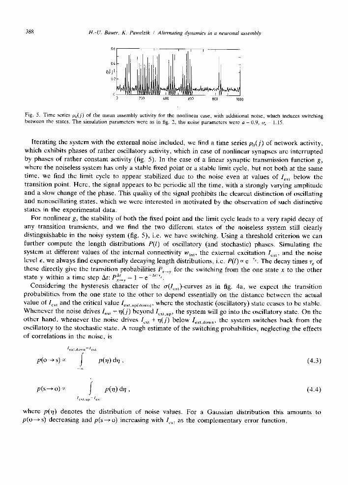
Fig. 5. Time series Po(J) of the mean assembly activity for the nonlinear case, with additional noise, which induces switching between the states. The simulation parameters were as in fig. 2, the noise parameters were a = 0.9, ~ = 1.15.

Iterating the system with the external noise included, we find a time series Po(J) of network activity, which exhibits phases of rather oscillatory activity, which in case of nonlinear synapses are interrupted by phases of rather constant activity (fig. 5). In the case of a linear synaptic transmission function g, where the noiseless system has only a stable fixed point or a stable limit cycle, but not both at the same time, we find the limit cycle to appear stabilized due to the noise even at values of Iex ~ below the transition point. Here , the signal appears to be periodic all the time, with a strongly varying amplitude and a slow change of the phase. This quality of the signal prohibits the clearcut distinction of oscillating and nonoscillating states, which we were interested in motivated by the observation of such distinctive states in the experimental data.

For nonlinear g, the stability of both the fixed point and the limit cycle leads to a very rapid decay of any transition transients, and we find the two different states of the noiseless system still clearly distinguishable in the noisy system (fig. 5), i.e. we have switching. Using a threshold criterion we can further compute the length distributions P( l ) of oscillatory (and stochastic) phases. Simulating the system at different values of the internal connectivity win,, the external excitation Iext, and the noise level e, we always find exponentially decaying length distributions, i.e. P( l ) o: e ~x. The decay times z x of these directly give the transition probabilities p~>. for the switching from the one state x to the other

A, e-a'/ra state y within a time step At: P x ~ v = 1 -

Considering the hysteresis character of the ~(Iext)-curves as in fig. 4a, we expect the transition probabilities from the one state to the other to depend essentially on the distance between the actual value of Iext and the critical value I¢~t,~p(Oow~), where the stochastic (oscillatory) state ceases to be stable. Whenever the noise drives Iext -{- T~(j) beyond I~xt,~p, the system will go into the oscillatory state. On the other hand, whenever the noise drives Iext + r/(j) below I~t,0 . . . . the system switches back from the oscillatory to the stochastic state. A rough estimate of the switching probabilities, neglecting the effects of correlations in the noise, is

lext ,down Iext

p(o---, s) ~ / p(r/) drl, (4.3)

p(s---~ o) ~ J p(r/) dr/, (4.4) lext .up - lext

where p(7/) denotes the distribution of noise values. For a Gaussian distribution this amounts to p ( o - ~ s) decreasing and p(s--~ o) increasing with Iext as the complementary error function,


012

010

008

005

00~

o

002

0 ~ ~' -16 1L

I I I I I o

o

o o

o o

o o

o o o o

I I ]" o

12 10 -08

l e x t

0 0 2 0 ~ I ' I I

t 0.015 ' P~ A i L

v 0005

o 0 06 -0~,

t I , I L I i

20 z.O flO 80 100 Aj

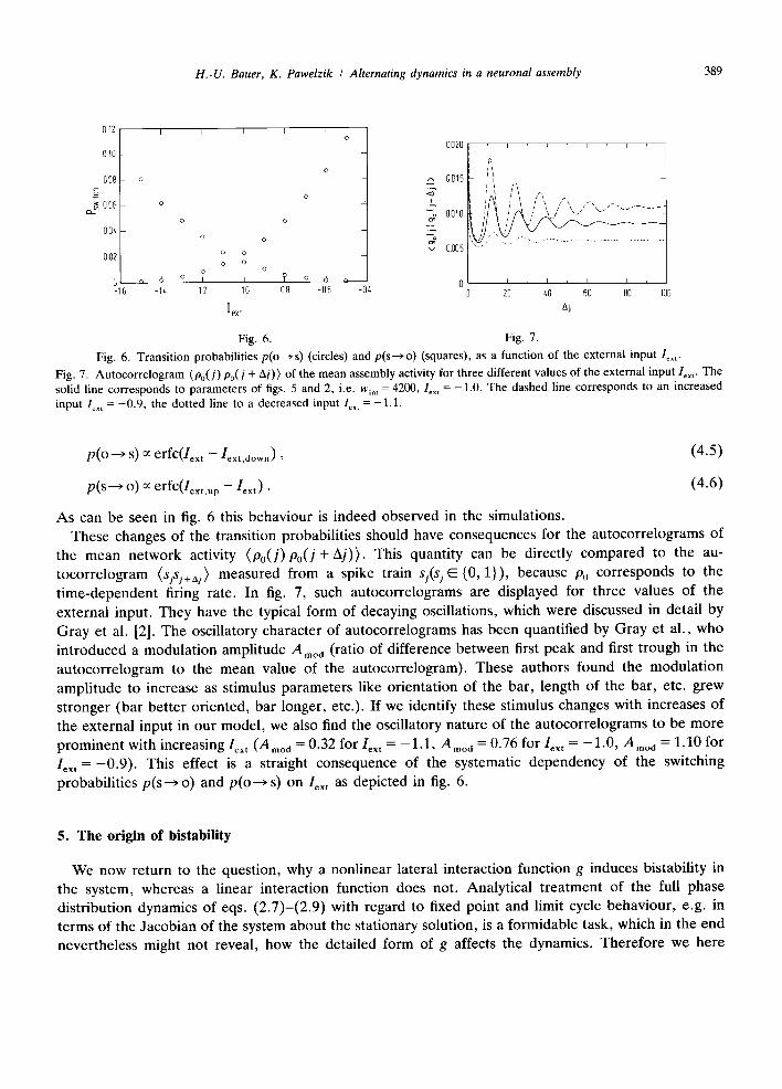
Fig. 6. Fig. 7. Fig. 6. Transition probabilities p(o ~ s) (circles) and p(s---~ o) (squares), as a function of the external input lox ,.

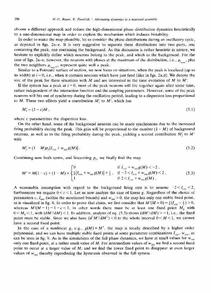
Fig. 7. Autocorrelogram (Po(J) Po(J + Aj)) of the mean assembly activity for three different values of the external input lex ,. The solid line corresponds to parameters of figs. 5 and 2, i.e. w~. t = 4200, le. , = -1.0. The dashed line corresponds to an increased input l~.t =-0 .9 , the dotted line to a decreased input lex t = -1.1.

p(o--> s) ~ erfc(Iex t - I e x t , d o w n ) , (4.5)

p(s--> o) ~ erfc(Iext,up - Iext) • (4.6)

As can be seen in fig. 6 this behaviour is indeed observed in the simulations. These changes of the transition probabilities should have consequences for the autocorrelograms of

the mean network activity (Po (J )Po(J + A j ) ) . This quantity can be directly compared to the autocorrelogram (sjsj+aj) measured from a spike train sj(sj E {0, 1}), because P0 corresponds to the t ime-dependent firing rate. In fig. 7, such autocorrelograms are displayed for three values of the external input. They have the typical form of decaying oscillations, which were discussed in detail by Gray et al. [2]. The oscillatory character of autocorrelograms has been quantified by Gray et al., who introduced a modulat ion amplitude A moa (ratio of difference between first peak and first trough in the autocorrelogram to the mean value of the autocorrelogram). These authors found the modulat ion amplitude to increase as stimulus parameters like orientation of the bar, length of the bar, etc. grew stronger (bar better oriented, bar longer, etc.). If we identify these stimulus changes with increases of the external input in our model , we also find the oscillatory nature of the autocorrelograms to be more prominent with increasing Iext ( A m o d = 0.32 for Iext = - 1 . 1 , Ar, oa = 0.76 for Iext : - 1 . 0 , A m o d = 1.10 for Iext = - 0 . 9 ) . This effect is a straight consequence of the systematic dependency of the switching probabilities p(s---> o) and p(o---> s) on Iext as depicted in fig. 6.

5. The origin of bistability

We now return to the question, why a nonlinear lateral interaction function g induces bistability in the system, whereas a linear interaction function does not. Analytical treatment of the full phase distribution dynamics of eqs. (2 .7 ) - (2 .9 ) with regard to fixed point and limit cycle behaviour, e.g. in terms of the Jacobian of the system about the stationary solution, is a formidable task, which in the end nevertheless might not reveal, how the detailed form of g affects the dynamics. Therefore we here


choose a different approach and reduce the high-dimensional phase distribution dynamics heuristically to a one-dimensional map in order to explain the mechanism which induces bistability.

In order to make the map plausible, let us consider the phase distributions during an oscillatory cycle, as depicted in figs. 2a -e . It is very suggestive to separate these distributions into two parts, one containing the peak, one containing the background. As this discussion is rather heuristic in nature, we hesitate to explicitly define which neurons belong to the peak, and which to the background. For the

case of figs. 2a - e , however, the neurons with phases at the maximum of the distribution, i.e., Pimax' plus the two neighbors Pim,,~l represent quite well a peak.

Similar to a Poincar6 surface of section, we now focus on situations, when the peak is localized (up to

its width) at i = 0, i.e., when it contains neurons which have just fired (like in figs. 2a,d). We denote the size of the peak for these situations with M and are interested in the time evolution of M to M'.

If the system has a peak at i = 0, most of the peak neurons will fire together again after some time, ra ther independent of the interaction function and the coupling parameters . However , some of the peak neurons will fire out of synchrony during the oscillation period, leading to a dispersion loss proport ional

to M. These two effects yield a contribution M' l to M', which has

M'~ = (1 - c)M, (5.1)

where c parametr izes the dispersion loss. On the other hand, some of the background neurons can be made synchronous due to the increased

firing probabil i ty during the peak. This gain will be proport ional to the number (1 - M) of background neurons, as well as to the firing probabili ty during the peak, yielding a second contribution M" to M ' with

M 2 = (1 - M)pi[l~x ~ + wi,tg(M)]. (5.2)

Combining now both terms, and linearizing pf, we finally find the map

1 l M ' = M(1 - c) + (1 - M) x [l~xt + wi°tg(M)] + 3 , if Iext + Wintg(M) < - 2 , if - 2 <lex t + wimg(M ) <2 , if 2 < lex t + wmtg(M ) .

(5.3)

A reasonable assumption with regard to the background firing rate is to assume - 2 < I e x t < 2 , fur thermore we require 0 < c < 1. Let us now analyze the case of linear g. Regardless of the choice of pa ramete rs c, Ic, t (within the ment ioned bounds) and wi, t > 0, the map has only one stable fixed point, as is visualized in fig. 8. In order to prove that claim, we first consider that M ' ( M = 0) - z - l (Iext + ½ ) > 0, whereas M'(M= 1 ) = l - c < 1, in other words there must be at least one fixed point M 0 with 0 < M 0 < 1, with (dM'/dM) < 1. In addition, analysis of eq. (5.3) shows (dM'/dM) > - 1 , i.e., the fixed point must be stable. Since we also have (d2M'/dM 2) < 0 in the whole interval 0 < M < 1, we cannot have a second fixed point.

In the case of a nonlinear g, e.g., g(M)= M 4, the map is locally described by a higher order polynomial , and we can have multiple stable fixed points at some paramete r combinations lex t, w~. t, as can be seen in fig. 9. As in the simulations of the full phase dynamics, we have at small values for Win t only one fixed point, at a rather small value of M. For intermediate values of wi, t we find a second fixed point to occur at a larger value of M, and we find the lower fixed point to disappear at even larger values of w~n t thereby reproducing the hysteresis observed in the full system.


1.0

0.8

06 H'

04

02

0 0

i i

I

02 0.4 0.6 08 10 M

1.0

08

06

0.4

02

0

i

02 0.4 0.6 08 10 H

Fig. 8. Fig. 9.

Fig. 8. 1D map (eq. (5.3)) describing the size M ' of the distribution peak after one cycle, as a function of the size M before the cycle. The interaction function g(M) is linear, resulting in a single stable fixed point of the map. The three curves correspond to three parameters for w~n , (wl, t = 1 (dashed), =3 (solid), =10 (dotted), le~ t = - 1 . 8 , c = 0.4). Each curve contains one stable fixed point of the map.

Fig. 9. As in fig. 8, but with a nonlinear interaction function g(M) = M 4. w~n t = 1 (dashed), =20 (solid), =400 (dotted). The intermediate curve has two stable fixed points (plus an unstable fixed point, which separates the basins of attraction).

6. Discussion

In this contribution we argued, that the variability in the time structure of cortical 40 Hz oscillations can be understood as a consequence of a bistability in the dynamics of the local neuronal substrate. The bistability emerges as a network property when the synaptic transmission is nonlinear. Fluctuations which may either stem from the input or from interaction with other assemblies then can switch between the costable dynamical states. In this discussion we would like to comment on a few aspects of this idea, which concern the relation of our approach to the experiments, to other theoretical work, and to functional consequences of a dynamics capable of switching.

Even though the alternating nature of the observed neuronal signals suggests a bistability of the underlying dynamics, it might be questionable, whether the switching between the stable states occurs at random, due to noise, or is a consequence of a functionally relevant processing mechanism. We feel the assumption of random fluctuations to be justified at this point, since the length distributions of the oscillatory periods observed in the experiments have an exponential distribution [5]. The length distribution of correlation events between two electrodes- which is very closely related to the distribution of the oscillatory periods themselves- also seems to be exponential [13]. In contrast, a functionally relevant mechanism which involves a specific time scale should be reflected by a characteristic peak in such a distribution. More complex mechanisms, so far beyond experimental control, could nevertheless be present. Because of the lack of knowledge about these interactions it appears justified to model these influences by fluctuations in the input too.

For the analysis of experimental data, autocorrelograms are the most favourite method. Our model reproduces not only the decaying oscillatory nature of the observed autocorrelograms- which can be regarded as the typical fingerprint of the 40 Hz oscillations - but also the variations of the modulation amplitude of the autocorrelograms which have been observed for varying stimulus parameters. Within the framework of the model, these variations result from the increased switching probability p(s--> o),


and the decreased probabili ty p(o--> s), which are manifest in longer oscillatory and shorter stochastic

periods. Considering that the increased modulat ion amplitude could as well be explained as a consequence of less frequency fluctuations with stronger inputs, the dependency of the switching probabili t ies on stimulus parameters constitutes a prediction of the model , which could be tested by

fur ther analysis with regard to the distinction of oscillatory and stochastic periods. The above arguments show, that autocorrelograms alone are not sufficient to fully characterize the

observed neuronal dynamics. This conclusion can also be drawn from a recent contribution by Koch and Schuster [22]. These authors showed, that the mere occurrence of noise-triggered bursts would be sufficient to induce an oscillatory component in the autocorrelation function of the neuronal signal. This is due to the fact that one burst cannot immediately be followed by a second burst, but requires some refractory period. In contrast to their approach, however, we assume that oscillatory periods indeed

consist of several periodically repeated firing events, and not just a single one. Last we would like to add a few comments on the possible functional consequences of considering the

oscillations as a transient dynamical phenomenon. Even though this seems to complicate matters at first glance, compared to ongoing oscillations, there might be a major advantage to the switching scenario. If a spatially extended system switches in unison from the stochastic to the oscillatory state due to a comm on input fluctuation, there is no time loss to establish spatial synchronicity. Such a fast synchronization is very desirable from a functional point of view, considering the speed of object recognition. In addition, an analysis of the crosscorrelation dynamics of responses f rom different sites in the cat cortex revealed, that synchrony can be established as fast as in a quarter oscillation period [13]. This t ime scale might be accessible to an array of simultaneously switching bistable elements, but it might be prohibitive for an array of permanent oscillators with synchronizing connections. The extension of our local model to a spatially extended system, and the investigation of the synchronization dynamics in such a system should therefore shed further light on the theoretical analysis of the binding

problem and the 40 Hz oscillation experiments.

Acknowledgements

This work has been supported by the Deutsche Forschungsgemeinschaft (Sonderforschungsbereich 185 "Nichtl ineare Dynamik" , TP A10, and Grant Ba 1105/3-1 to H U B ) and by a grant of the Stiftung

Volkswagenwerk.

References

[1] C.M. Gray, P. K6nig, A.K. Engel and W. Singer, Nature 338 (1989) 334. [2] C.M. Gray, A.K. Engel, P. K6nig and W. Singer, Eur. J. Neurosci. 2 (1990) 607. [3] R. Eckhorn, R. Bauer, W. Jordan, M. Brosch, W. Kruse, M. Munk and H.J. Reitb6ck, Biol. Cyb. 60 (1988) 121. [4] A.K. Kreiter and W. Singer, Eur. J. Neurosci. 4 (1992) 369. [5] V.N. Murthi and E.E. Fetz, Proc. Natl. Acad. Sci. USA 89 (1991) 5670. [6] C. v.d. Malsburg, The correlation theory of brain function, Internal Report MPI ffir biophysikalische Chemie 81-2 (1981). [7] C. v.d. Malsburg and J. Buhmann, Biol. Cyb. 67 (1992) 233. [8] T.B. Schillen and P. K6nig, Neural Comput. 3 (1991) 167. [9] P. K6nig and T.B. Schillen, Neural Comput. 3 (1991) 155.

[10] E. Niebur, D. Kammen and C. Koch, in: Nonlinear Dynamics and Neuronal Networks, ed. H.-G. Schuster (Verlag Chemic, Weinheim, 1990) p. 173.

[11] H.-G. Schuster and E Wagner, Biol. Cyb. 64 (1990) 77.


[12] H.-G. Schuster and P. Wagner, Biol. Cyb. 64 (1990) 83. [13] C.M. Gray, A.K. Engel, P. K6nig and W. Singer, Vis. Neurosci. 8 (1992) 337. [14] C.M. Gray, A.K. Engel, P. K6nig and W. Singer, in: Nonlinear Dynamics and Neuronal Networks, ed. H.G. Schuster,

(Verlag Chemie, Weinheim, 1990) pp. 27-55. [15] K. Pawelzik, H.-U. Bauer and T. Geisel, Proc. CNS 92 San Francisco (Kluwer, Dordrecht) in print. [16] Y. Kuramoto, Physica D 50 (1991) 15. [17] D.E. Rumelhart and J.L. McClelland, Parallel Distributed Processing (MIT Press, Cambridge, MA, 1986). [18] D.H. Perkel, G.L. Gerstein and G.P. Moore, Biophys. J. 7 (1967) 391. [19] W. Gerstner and L. van Hemmen, Network 3 (1992) 139. [20] A.L. Hodgkin and A.F. Huxley, J. Physiol. (London) 117 (1952) 500. [21] R.R. Llinas, Science 242 (1988) 1654. [22] C. Koch, H.-G. Schuster, Neural Comput. 4 (1992) 211.

Documents

Alternating oscillatory and stochastic dynamics in a model for a neuronal assembly